Analysing the influence of upslope bedrock outcrops …intra.tesaf.unipd.it/people/tarolli/Papers/Tarolli et al. (2008).pdfAnalysing the influence of upslope bedrock outcrops on shallow

Available online at www.sciencedirect.com

2008) 186–200www.elsevier.com/locate/geomorph

Geomorphology 93 (

Analysing the influence of upslope bedrockoutcrops on shallow landsliding

Paolo Tarolli ⁎, Marco Borga, Giancarlo Dalla Fontana

Department of Land and Agroforest Environments, University of Padova, Agripolis, viale dell’Università 16, 35020 Legnaro (PD), Italy

Received 30 June 2006; received in revised form 21 February 2007; accepted 23 February 2007Available online 6 March 2007

Abstract

A model for the prediction of topographic and climatic control on shallow landsliding in mountainous terrain is enhanced toanalyse the impact of upslope rocky outcrops on downslope shallow landsliding. The model uses a ‘generalised quasi-dynamicwetness index’ to describe runoff propagation on bare rock surfaces connected to downslope soil-mantled topographic elements.This approach yields a simple enhanced model capable of describing the influence of upslope bedrock outcrops on the pattern ofdownslope soil saturation. The model is applied in both diagnostic and predictive modes to a small catchment in the eastern ItalianAlps for which a detailed inventory of shallow landslides in areas dominated by rocky outcrops is available. In the diagnosticmode, the model is used with satisfactory results to reproduce the pattern of instability generated by an intense short-duration stormoccurred on 14 September 1994, which triggered a large percentage of the surveyed landslides. In the predictive mode, the model isused for hazard assessment, and the return time of the critical rainfall needed to cause instability for each topographic element isdetermined. Modelling results obtained in the predictive mode are evaluated against all the surveyed landslides. It is revealed thatthe generalised quasi-dynamic model offers considerable improvement over the non-generalised quasi-dynamic model and thesteady-state model in predicting existing landslides as represented in the considered landslide inventory.© 2007 Elsevier B.V. All rights reserved.

Keywords: Shallow landslides; Bedrock outcrops; Alps; Subsurface flow; Surface flow; Debris flow

1. Introduction

Rainfall and site-specific factors such as soil thickness,material properties, and root cohesion influence the spatialdistribution of potential slope stability (Wilson andDietrich, 1987; Reid and Iverson, 1992; Iverson et al.,1997; Montgomery et al., 1997; Roering et al., 2003). InhumidAlpine landscapes, where shallow landsliding is theprimary erosional process, bedrock outcrops can play animportant role in the activation of slope instability

⁎ Corresponding author. Tel.: +39 049 8272695; fax: +39 049 8272686.E-mail address: [email protected] (P. Tarolli).

0169-555X/$ - see front matter © 2007 Elsevier B.V. All rights reserved.doi:10.1016/j.geomorph.2007.02.017

(Haeberli et al., 1990; Wilkenson and Schmid, 2003;Glade, 2005).Most slope failures and debris flows in steepAlpine regions occur in areas where topographic condi-tions provide a debris source from cliff faces and anaccumulation of regolith, often in the form of talus slopes(either vegetated or not). Upslope rock walls are the watercatchments and sediment sources for these shallowlandslides. Water and sediments, concentrated alongsmall steep drainage lines, flow onto the slopes at thebase of the bedrock area, possibly eroding and transportingmaterial downslope. The coarse sediment of talus depositshas a large porosity and consequently high infiltrationcapacity. Owing to these reasons, the flow infiltrates rather

mailto:[email protected]

http://dx.doi.org/10.1016/j.geomorph.2007.02.017

Fig. 1. Runoff from bedrock outcrops infiltrates into a vegetated talus deposit observed in the Dolomite, the Eastern Italian Alps.

187P. Tarolli et al. / Geomorphology 93 (2008) 186–200

quickly in the sediment and enhances the saturation of theunconsolidated colluvium wedge at the base of cliffs,triggering slope instability and debris flow processes. Anexample is shown in Fig. 1 where the overland flow fromsteep rock gullies infiltrates into a vegetated talus deposit atthe base of cliffs. Empirical observations suggest thatshallow landslides in these landscape elements are lessinfluenced by previous soil moisture conditions and maybe triggered by storms of shorter duration and higherintensity, compared to landscape elements draining soil-mantled hollows.When scree deposits are topographicallyconnected to steep creeks, as happens in many alpinelandscapes, debris flows from landslides can travel manyhundreds ofmeters. This represents awidespread source ofhazard and risks in alpine regions (Haeberli et al., 1990;Villi and Dal Prà, 2002).

The main objective of this paper is to describe and testa model of shallow landsliding (called hereafter ‘Gener-alised Quasi-Dynamic Model’ or ‘Generalised QDM’)capable of describing the influence of upslope bedrockoutcrops on the pattern of downslope soil saturation andlandsliding susceptibility. The model is built upon atheory of coupled dynamic shallow subsurface flow andlandsliding proposed byBorga et al. (2002a), which uses a‘quasi-dynamic wetness index’ to predict the spatialdistribution of soil saturation in response to a rainfall ofspecified duration. With the Generalised QDM, the quasi-dynamic wetness index is generalised to describe surfaceand subsurface runoff propagation on various surfacetypes, including bare rock and soil-mantled elements. The

Generalised QDM is coupled with a simple scaling modelof extreme rainfall, to provide a compact description ofclimatic and topographic controls on shallow landsliding.The model is applied and tested on the upper Rio Cordonbasin (1.47 km2), a mountainous catchment in theDolomites region, where field surveys provide a descrip-tion of hydraulic and geotechnical properties of soils, andan inventory of landslide scars is available. Themethodology developed by Borga et al. (2002a) for thecomparison of slope-stability index models is used tocompare the results provided by the Generalised QDMwith those obtained by the quasi-dynamic model and thesteady-state model (Montgomery and Dietrich, 1994).

2. Methodology

Montgomery and Dietrich (1994) developed a simplemodel for the topographic influence on shallow landslideinitiation, by coupling digital terrain data with near-surface throughflow and slope-stability models. Theirapproach is based on a steady-state assumption implyingthat the specific upslope area is a surrogate measure ofsubsurface flow at any point in the landscape. However,this is only valid if recharge to a perched water tableoccurs for the length of time required for every point alongthe hillslope to reach subsurface drainage equilibrium andexperience drainage from its entire upslope contributingarea (Barling et al., 1994).

Borga et al. (2002a) developed a slope-stability model(called ‘Quasi-Dynamic Model’ or ‘QDM’ hereafter)

188 P. Tarolli et al. / Geomorphology 93 (2008) 186–200

which takes transient movement of soil water intoaccount. The QDM is based on a quasi-dynamic wetnessindex which takes into consideration the time forsubsurface water to redistribute across the catchmentand yet maintains the simplicity of the index approach.For each element and for a user-specified drainageperiod, a set of points upslope of that element whichcontributes flow within the specified drainage period iscomputed using the quasi-dynamic wetness index. Thisyields a simple model capable of incorporating thecombined effect of storm duration and intensity in thetriggering mechanism of shallow landslides.

When the upper portions of the landscape arecharacterised by bedrock outcrops, the quasi-dynamicmodel needs to be generalised in order to take account ofdifferent runoff propagation velocities through the barerock and the soil-mantled topographic elements. Thissection firstly shows how the kinematic wave model forsubsurface and surface flow can be used to derive thegeneralised quasi-dynamic wetness index. Then, thegeneralised quasi-dynamic wetness index is coupledwith the Coulomb failure approach (Borga et al., 2002b)to provide the Generalised QDM slope-stability model.

2.1. Kinematic wave and the generalised quasi-dynamicwetness index

The kinematic wave formulation is based on theassumption that the hydraulic gradient at any point withinthe saturated zone is equal to the bed slope. Beven (1981,1982a,b) demonstrated that the kinematic wave assump-tion is an acceptable approximation to the theoreticallymore complete Dupuit–Forchheimer equation as theeffective hydraulic conductivity and bed slope increases.The kinematic wave equation, generalised to incorporatethe effects of downslope convergence and divergence, isgiven by

AQss

Axþ AQss

Ate

K sin h cos h¼ r tð Þw xð Þ ð1Þ

Qss ¼ KS1e

sin h ð2Þ

whereS1 [L2] is the soilmoisture capacity defined asS1(x)=

w (x)h (x)ε, with w (x) being the contour length [L] at ahorizontal downslope distance of x [L], h(x) [L] thethickness of the saturated region above the bed measuredperpendicular to the bed at x, and ε [−] the drainableporosity; θ is the local topographic slope, Qss [L

3 T −1] isthe subsurface flow discharge, K [L T −1] is the effectivehydraulic conductivity assumed constant with depth, and

r (t) [L T −1] is the rainfall rate measured per unit planararea at time t [T ]. It is assumed here that the rainfall rateequals the recharge which passes through (or bypasses)the unsaturated zone to reach the saturated zone andeventually become subsurface runoff.

The equation describing the kinematic wavemodel canbe transformed to a set of ordinary differential equationsvalid along characteristic curves by the method ofcharacteristics. The kinematic wave equation has onlyone set of characteristics, which in the absence of shocksis described everywhere in the (x,t) plane as

css ¼ dxdt

¼ K sin h cos he

ð3Þ

where css represents the celerity of the subsurfacekinematic wave.

Along the characteristic line, Eq. (1) becomes

dQss

dx¼ r tð Þw xð Þ: ð4Þ

For the case of overland flow, the kinematic waveequation is given by

AQs

Axþ AQs

At1

C sin h cos h¼ r tð Þw xð Þ ð5Þ

Qs ¼ Cw xð Þy xð Þ sin h ¼ CS2 sin h ð6Þ

where y(x) [L] is the overland flow depth measuredperpendicular to the surface, Qs [L

3 T −1] is overlandflow discharge, S2 [L2] denotes the overland watercapacity and C [L T −1] is overland flow conductance.Eqs. (5) and (6) are based on the following twosimplifications: (i) kinematic approximation — theenergy slope is replaced by the bedrock or terrain slope(they are assumed to be the same), and (ii) the overlandflow is described based on a linear equation. Since theoverland flow along bedrock outcrops is likely to beshallow, a porous media approximation may not becompletely unrealistic. However, Cmust be greater thanK, as much as 300–500 times, as observed by Dunneand Black (1970).

Along the overland flow characteristic line, theoverland flow kinematic equation becomes

dQs

dx¼ r tð Þw xð Þ ð7Þ

when the line is given in the (x,t) plane by

cs ¼ dxdt

¼ C sin h cos h ð8Þ


where cs represents the celerity of the surface kinematicwave.

Under the assumptions that i) the surface runoff istransformed completely to subsurface flow on the talusdeposit, ii) rainfall and recharge rates are constant intime and space, and iii) initial flow is zero, the dischargeQss(d ) and the flow depth h(d ) at the end of the rainfalltime d can be written respectively by

Qss dð Þ ¼ r0AGQD dð Þ ð9Þand

h dð Þ ¼ minr0

w dð ÞK sin hAGQD dð Þ; z

� �

¼ minr0K sin h

aGQD dð Þ; zh i

ð10Þ

where r0 [L T −1] is the constant rainfall rate, z [L] isthe soil depth measured perpendicular to the bed, andAGQD(d ) [L

2] is the fraction of the specific contributingarea (measured along the horizontal plane) whichcontributes flow (both as surface and subsurface flow)to the contour segment length within the specifieddrainage period taken equal to the storm duration d:

AGQD dð Þ ¼Z x dð Þ

0w xð Þdx ð11Þ

with x(d ) being the distance computed along thecharacteristic line during the time interval d, and aGQD(d) [L] is the specific contributing area per unit contourlength within the period d. The areaAGQD(d) may includeboth soil-mantled terrain as well as bedrock outcrops.

In the following, we will identify the ratio aGQD(d)/sinθ as the generalised quasi-dynamic wetness index(called hereafter Generalised QDWI). Alternative formsof the wetness index are the quasi-dynamic wetness index(QDWI) computed with reference only to the subsurfaceflow, and the steady-state wetness index (Montgomeryand Dietrich, 1994). The procedure described in Borgaet al. (2002a) has been used here for the computation ofthe Generalised QDWI, by using different local celeritiesfor bare rock surfaces and soil-mantled elements.

Given the same landscape topography and the samerainfall duration d, the presence of bedrock outcrops willincrease the specific contributing area for those topo-graphic elements located downslope of the bedrockoutcrops, owing to the wide difference between thevalues of the parametersK andC. However, the differencewill depend upon the rainfall duration, since for durationsequal to or longer than the time required to reachsubsurface drainage equilibrium, the contributing area

will be the same for the generalised and quasi-dynamicprocedure. In essence, therefore, the Generalised QDWIallows one to identify the topographic elements as well asthe rainfall duration most susceptible to subsurface flowenhancement due to upslope bedrock outcrops.

2.2. The coupled hydrologic and slope-stability model

Coupling the hillslope hydrology model with geo-mechanics yields a model of landslide triggering byprecipitation. The subsurface flow model incorporatingthe Generalised QDWI is coupled with a planar infiniteslope, Coulomb failure model of a cohesionless soil ofconstant thickness and slope, to identify unstabletopographic elements in a way conceptually similar tothat proposed by Montgomery and Dietrich (1994) andBorga et al. (2002a). We will assume here that the entiresoil profile is initially wet to field capacity.

For cohesionless material and slope parallel seepage,the infinite slope-stability model can be written as

qsz tan h ¼ qwz−qshð Þ tan / ð12Þwhere ρs and ρw [M L−3] are soil (including the masscontribution from soil moisture) and water density,respectively, and ϕ is the soil internal friction angle. It isimportant to recognise that all forces in infinite slopesare assumed to vary only in the direction normal to theground surface. This precludes accurate assessment ofslopes in which subsurface flow or topography producesforces that vary in directions other than the slope-normalone. Eq. (12) may be rewritten as follows

hz¼ qs

qw1−

tan htan /

� �: ð13Þ

Substitution of Eq. (10) into Eq. (13) allows thisfailure criterion to be expressed in terms of specificdrainage area per unit contour length, computedaccordingly with the generalised quasi-dynamic theory.Thus the following relationship is used to identifyunstable topographic elements

aGQD dð Þz Tr dð Þ sin h

qsqw

1−tan htan /

� �ð14Þ

where T [L2 T −1] represents the soil transmissivity,taken equal to K · z, and r(d ) [L T −1] is the rainfall ratefor storm duration d.

According to Montgomery and Dietrich (1994), fourslope-stability classes can be defined: unconditionallyunstable, unstable, stable, unconditionally stable.Ground is unconditionally unstable if it is unstable


even when dry, i.e. when tanθN tanϕ. Unstable elementsare those predicted to fail according to Eq. (14). Stableelements have an upslope effective contributing area orrainfall rate insufficient for their failure, but slopes steepenough to fail if they become saturated. Unconditionallystable elements are those predicted to be stable evenwhen saturated; this condition is written as

tan hb tan / 1−qwqs

� �: ð15Þ

Topographic elements which are neither uncondi-tionally unstable nor unconditionally stable will becalled conditionally unstable in the following. Forconditionally unstable elements, the stability thresholdidentified by Eq. (14) might be crossed by increasing therainfall rate r for constant duration storms and/or byincreasing the contributing area, which means increas-ing the storm duration. Once this threshold is crossed, anelement will remain unstable at greater rainfall rates or atlonger storm duration. It is therefore possible todetermine for each storm duration d and for eachelement the minimum uniform rainfall needed to causeinstability, called critical rainfall rate r

cr(d ), by rearran-

ging Eq. (14):

rcr dð Þ ¼ T sin haGQD dð Þ

qsqw

1−tan htan /

� �: ð16Þ

Eq. (16) extends the definition of critical rainfallprovided by Montgomery and Dietrich (1994), andenhances the model developed by Borga et al. (2002a)by taking the role of bedrock outcrops into account.

2.3. Diagnostic and predictive procedures for modelapplications

Two general procedures may be considered formodel application: diagnostic and predictive. With thefirst procedure, topographic element stability is simu-lated for a given temporal pattern of rainfall intensityand for given initial soil moisture conditions. Thisallows us to explore the pattern of instability generatedby specific storms and to evaluate the model bycomparing the simulated instability with one triggeredby a storm. A model application with input from a givenprecipitation time series needs to take into account theassumption of time–space constant rainfall used formodel derivation. For this purpose, the precipitationtime series r(i), i=1,N , n, with d=n▵t, ▵t being themeasurement time step, is approximated by a sequenceof time-constant precipitations with intermediate dura-

tion ranging from one time step to the duration of theconsidered storm. The average rainfall intensity raveused for each intermediate duration is computed as

rave; j ¼Pji¼1

r ið ÞDtjDt

; j ¼ 1; N ;dDt

: ð17Þ

For each intermediate duration, the stability ofconditionally unstable elements is evaluated by com-paring the average rainfall intensity computed by meansof Eq. (17) and the critical rainfall intensity obtainedthrough Eq. (16). The pattern of simulated instabilitytriggered by the storm is given by the ensemble of theinstability computed for each intermediate duration.

In the predictive mode, the lowest return time of thecritical rainfall is computed for each conditionallyunstable cell in the landscape. The computation isbased on Eq. (16), which relates the critical rainfall withits duration, and on the availability of an Intensity-Duration-Frequency relationship (hereafter referred toas IDF) for the study area, which provides a return timefor a given association of rainfall rate and stormduration. For each conditionally unstable cell, the returntime of the critical rainfall is computed for a range ofstorm duration. Then, the lowest return time is selected.All points with the same value of return time of criticalrainfall have equal topographic and climatic control onshallow landslide initiation. A map of the return time ofthe critical rainfall provides therefore a representation ofthe susceptibility to shallow landsliding across thelandscape. As such, the predictive mode of modelapplication is most useful for hazard assessment. Aformulation for the computation of the return time of thecritical rainfall is provided below.

The IDF relationship commonly used in Italy isexpressed by a power function

rF dð Þ ¼ 1FdmF−1 ð18Þ

where rF is the rainfall rate which can be exceeded witha probability of (1−F ), and ςF and mF are parametersestimated by least squares regression of rF against stormduration d.

In contrast to the empirical approach, which dependson curve-fitting techniques, Burlando and Rosso (1996)in a pioneering paper sought to apply the scalinghypotheses to the IDF relationship. In their work thescaling and multiscaling properties of the statisticalmoments of rainfall depth of different duration wereanalyzed, and a lognormal probability distribution wasused to model its statistical properties.


Borga et al. (2005) showed that a Gumbel simplescaling model describes well the distribution of annualmaximum series of rainfall in a region of the CentralItalian Alps. Based on this model, the rainfall rate rF (d )can be determined as

rF dð Þ ¼ 11 1−CVffiffiffi6

p

pnþ yTrð Þ

� �dm−1 ð19Þ

with ς1 (L T1−m) denoting the expected value of annualmaximum rainfall depth for the unit duration, m thescaling exponent, ξ the Euler's constant (approximately0.5772), CV the coefficient of variation, assumedconstant with the different durations, and yTr the Gumbelreduced variable as

yTr ¼ ln lnTr

Tr−1

� �� ð20Þ

with Tr being the return time, i.e., 1 / (1−F ). The valuesof ς1 and m can be estimated by linear regression of therelationship between rainfall depth and duration, afterlog transformation, whereas the value of CV can beobtained as the average of the coefficient of variationcomputed for different durations, in a range for whichthe scaling property holds.

Combination of Eqs. (16) and (19) yields thefollowing critical value for yTr,

yTr ¼ pffiffiffi6

p 1CV

1−T sin haGQD dcrð Þ

qsqw

1−tan htan /

� �d 1−mcr

11

� �−n:

ð21Þ

Therefore, the critical duration dcr is the duration whichminimizes the value of yTr accordingly with Eq. (21).After the computation of yTr, the value of return time canbe determined by inverting Eq. (20).

Eq. (21) incorporates in a compact way the climatecontrol (represented by parameters ς1, CV and m) onshallow landsliding. The quality of the model representa-tion of susceptibility to landsliding, as obtained in thepredictive mode, can be assessed by comparing thelocations of all observed landslides (not only thosetriggered by specific storms, as done in the diagnosticmode) with model predictions. The comparison is obtainedby plotting observed landslides on amap of predicted returntime of critical rainfall, and comparing the proportion ofcatchment area placed in various return time ranges to thecorresponding fraction of the landslide area.

It is important to note that values of return timeprovided by the model may not represent the return timeof landsliding. The landslide return time is not only

related to the precipitation return time but also to hollowinfilling time, which controls the regeneration ofcolluvial wedges following their partial or total removalduring an event. To estimate the landsliding return time,a coupled model of soil depth development andrainstorm occurrence is necessary, since both of themcontrol the recurrence interval of shallow landsliding(Iida, 1999). These considerations therefore illustratethat the primary model result is a relative rating ofpotential instability. Hence a short return time of criticalrainfall means least stable, and a long return time meansmost stable.

3. Study area and model application

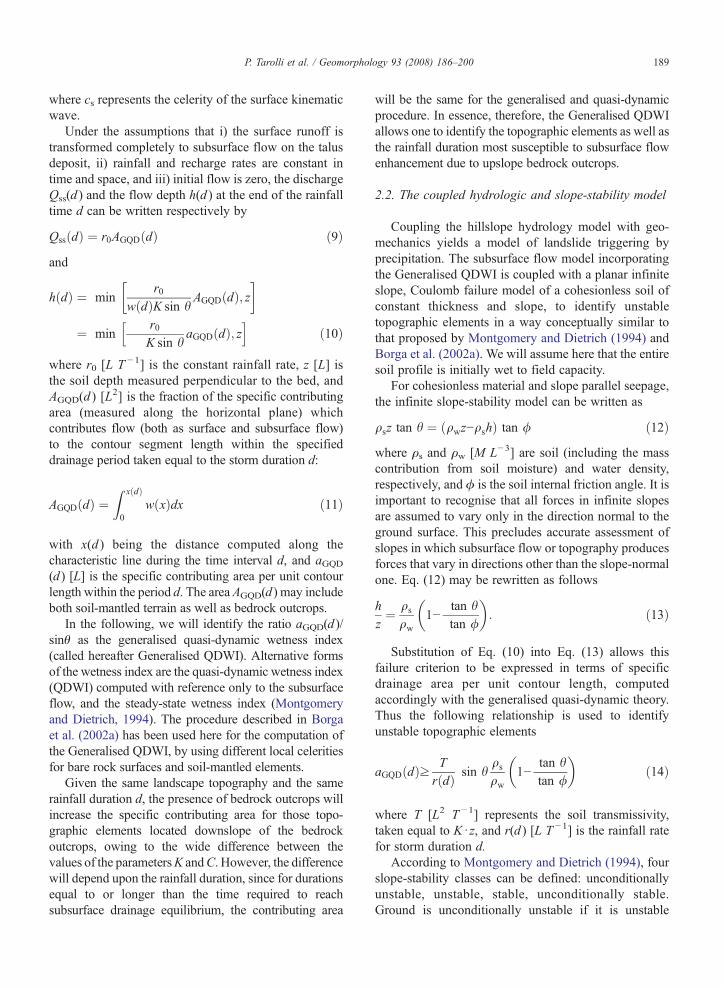
The study area is the upper Cordon basin (1.47 km2),located in the Dolomites, in the Eastern Italian Alps(Fig. 2A). The elevation ranges from2130 to 2706m a.s.l.,with an average of 2340m a.s.l. The average slope angle is25°. In this basin mountain summits consist of dolomitesmaking up subvertical cliffs. These cliffs are bordered byscree slopes consisting of relatively coarse, unconsolidat-ed rock debris, in the form of vegetated talus deposits(Fig. 1), and colluvium wedges. The area has a typicalAlpine climate with a mean annual rainfall of about1100 mm. Precipitation occurs mainly as snowfall fromNovember to April. Runoff is dominated by snowmelt inMay and June, but summer and early autumn floodsrepresent an important contribution to the flow regime.During summer, storm events are usually intervalled bylong dry spell. During these events several shallowlandslides are triggered on steep screes at the base of cliffs.Soil thickness varies between 0.2 and 0.5 m ontopographic spurs to depths of up 1.5 m on topographichollows. High altitude grassland covers 61% of the area(in which 30% is vegetated talus deposits). The remaining39% of the area is bedrock outcrops (28%), unvegetatedtalus deposits (10%), and unvegetated landslide scars(1%).

Almost all shallow landsliding in this area occurs onunconsolidated talus slopes below bedrock outcrops.The mapped landslide area amounts to 1% of the totalstudy area, with an average slope of 41°. These datawere documented by repeated field surveys during theperiod 1992–2001 (Borga et al., 1998, 2002b). InFig. 2B, only the landslide initiation areas as clustersof initiation points are represented using polygons. Asis evident from Fig. 2B, local topography andconnection with rocky outcrops control the positionsof landslides. Many landslides are concentrated imme-diately below local occurrences of rocky outcrops. Nolandslides are located on less steep scree slopes. Almost


all mapped landslides transformed to debris flows, withvolumes ranging from some tens to two hundred cubicmeters.

Ten scree slopes were randomly selected for analysisof physical characteristics of their deposits. Most slopesselected are vegetated talus slopes, since a higherpercentage of landslides were observed on them.Samples for analysis were taken from 30 to 50 cmbelow the surface. The graphic mean grain diameter(Folk, 1965) was estimated to be −1.8±1.05 in φ units.Bulk density was determined in the field by theexcavation method, and total porosity was calculatedfrom bulk density after particle density of rock fragmentswas measured (2.72 g cm−3). On scree slopes, internalfriction angle was evaluated following the proceduredescribed by Blijenberg (1995).

Fig. 2. Study area. A) Map showing the location of the study area; B) map shoof cliffs; C) map showing the landslides triggered by the storm occurred on

About 68% of the surveyed landslides were triggeredby a very intense and short-duration storm on 14 Septem-ber 1994 (Lenzi, 2001; Lenzi et al., 2004) (Fig. 2C). Thestorm, with a duration of 6 h, caused the largest floodrecorded in 20 years of observation in the Rio Cordonbasin. Due to the short duration of the storm, few slopeinstabilities were observed on entirely soil-covered slopes,while several landslides were triggered on slopes justbelow rocky outcrops.

Model parameters evaluated based on field measure-ments are shown in Table 1 for two different land units:talus deposit and soil-mantled slopes. The flow conduc-tance on rocky outcrops was assumed to be 1 m s−1.

For characterising the IDF relationship at the site,annual maximum rainfall data of 1, 3, 6, 12, and 24 h, andof 1 to 5 consecutive days were collected from records at

wing the bedrock outcrops and the analyzed landslides areas at the base14 September 1994. Contour interval in (B) and (C) is 50 m.

Fig. 2 (continued ).


the station located in Caprile, close to the study area, andowned by the Italian Hydrological Service. These datawere elaborated following the Gumbel distribution andthe simple scaling assumption, which has been shown to

hold for this region (Borga et al., 2005). The followingparameters were estimated for application of Eq. (19):ς1=16.47 mm h1−0.48, CV=0.31, and n=0.48. Thegeneralised quasi-dynamic wetness index was computed

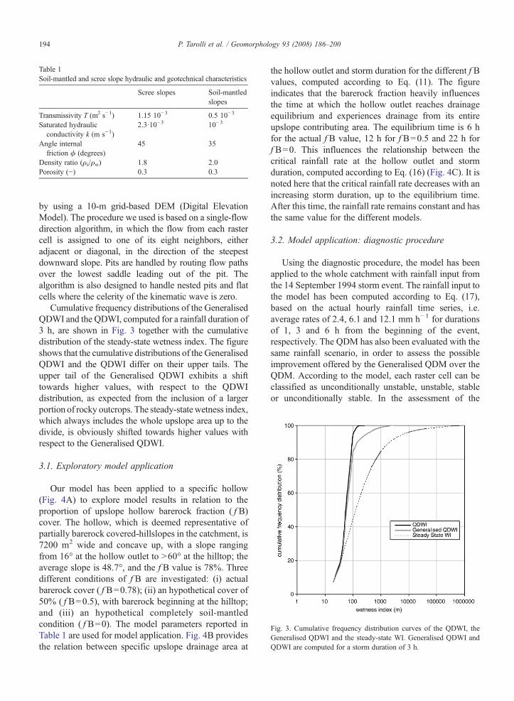
Table 1Soil-mantled and scree slope hydraulic and geotechnical characteristics

Scree slopes Soil-mantledslopes

Transmissivity T (m2 s−1) 1.15 10−3 0.5 10−3

Saturated hydraulicconductivity k (m s−1)

2.3·10−3 10−3

Angle internalfriction ϕ (degrees)

45 35

Density ratio (ρs/ρw) 1.8 2.0Porosity (−) 0.3 0.3

Fig. 3. Cumulative frequency distribution curves of the QDWI, theGeneralised QDWI and the steady-state WI. Generalised QDWI andQDWI are computed for a storm duration of 3 h.


by using a 10-m grid-based DEM (Digital ElevationModel). The procedure we used is based on a single-flowdirection algorithm, in which the flow from each rastercell is assigned to one of its eight neighbors, eitheradjacent or diagonal, in the direction of the steepestdownward slope. Pits are handled by routing flow pathsover the lowest saddle leading out of the pit. Thealgorithm is also designed to handle nested pits and flatcells where the celerity of the kinematic wave is zero.

Cumulative frequency distributions of the GeneralisedQDWI and the QDWI, computed for a rainfall duration of3 h, are shown in Fig. 3 together with the cumulativedistribution of the steady-state wetness index. The figureshows that the cumulative distributions of the GeneralisedQDWI and the QDWI differ on their upper tails. Theupper tail of the Generalised QDWI exhibits a shifttowards higher values, with respect to the QDWIdistribution, as expected from the inclusion of a largerportion of rocky outcrops. The steady-statewetness index,which always includes the whole upslope area up to thedivide, is obviously shifted towards higher values withrespect to the Generalised QDWI.

3.1. Exploratory model application

Our model has been applied to a specific hollow(Fig. 4A) to explore model results in relation to theproportion of upslope hollow barerock fraction ( f B)cover. The hollow, which is deemed representative ofpartially barerock covered-hillslopes in the catchment, is7200 m2 wide and concave up, with a slope rangingfrom 16° at the hollow outlet to N60° at the hilltop; theaverage slope is 48.7°, and the f B value is 78%. Threedifferent conditions of f B are investigated: (i) actualbarerock cover ( f B=0.78); (ii) an hypothetical cover of50% ( f B=0.5), with barerock beginning at the hilltop;and (iii) an hypothetical completely soil-mantledcondition ( f B=0). The model parameters reported inTable 1 are used for model application. Fig. 4B providesthe relation between specific upslope drainage area at

the hollow outlet and storm duration for the different f Bvalues, computed according to Eq. (11). The figureindicates that the barerock fraction heavily influencesthe time at which the hollow outlet reaches drainageequilibrium and experiences drainage from its entireupslope contributing area. The equilibrium time is 6 hfor the actual f B value, 12 h for f B=0.5 and 22 h forf B=0. This influences the relationship between thecritical rainfall rate at the hollow outlet and stormduration, computed according to Eq. (16) (Fig. 4C). It isnoted here that the critical rainfall rate decreases with anincreasing storm duration, up to the equilibrium time.After this time, the rainfall rate remains constant and hasthe same value for the different models.

3.2. Model application: diagnostic procedure

Using the diagnostic procedure, the model has beenapplied to the whole catchment with rainfall input fromthe 14 September 1994 storm event. The rainfall input tothe model has been computed according to Eq. (17),based on the actual hourly rainfall time series, i.e.average rates of 2.4, 6.1 and 12.1 mm h−1 for durationsof 1, 3 and 6 h from the beginning of the event,respectively. The QDM has also been evaluated with thesame rainfall scenario, in order to assess the possibleimprovement offered by the Generalised QDM over theQDM. According to the model, each raster cell can beclassified as unconditionally unstable, unstable, stableor unconditionally stable. In the assessment of the

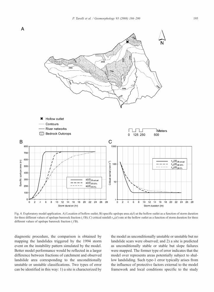
Fig. 4. Exploratory model application. A) Location of hollow outlet; B) specific upslope area a(d ) at the hollow outlet as a function of storm durationfor three different values of upslope barerock fraction ( f B); C) critical rainfall rcr(d ) rate at the hollow outlet as a function of storm duration for threedifferent values of upslope barerock fraction ( f B).


diagnostic procedure, the comparison is obtained bymapping the landslides triggered by the 1994 stormevent on the instability pattern simulated by the model.Better model performance would be reflected in a largerdifference between fractions of catchment and observedlandslide area corresponding to the unconditionallyunstable or unstable classifications. Two types of errorcan be identified in this way: 1) a site is characterized by

the model as unconditionally unstable or unstable but nolandslide scars were observed; and 2) a site is predictedas unconditionally stable or stable but slope failureswere mapped. The former type of error indicates that themodel over represents areas potentially subject to shal-low landsliding. Such type-1 error typically arises fromthe influence of protective factors external to the modelframework and local conditions specific to the study

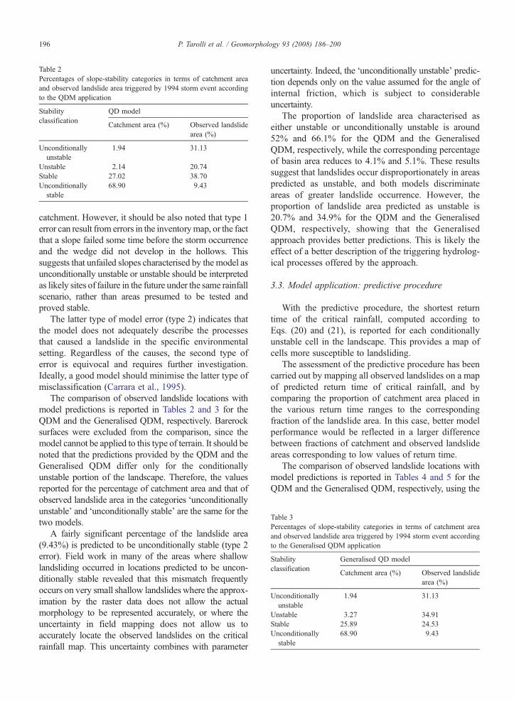
Table 2Percentages of slope-stability categories in terms of catchment areaand observed landslide area triggered by 1994 storm event accordingto the QDM application

Stabilityclassification

QD model

Catchment area (%) Observed landslidearea (%)

Unconditionallyunstable

1.94 31.13

Unstable 2.14 20.74Stable 27.02 38.70Unconditionallystable

68.90 9.43

Table 3Percentages of slope-stability categories in terms of catchment areaand observed landslide area triggered by 1994 storm event accordingto the Generalised QDM application

Stabilityclassification

Generalised QD model



1.94 31.13

Unstable 3.27 34.91Stable 25.89 24.53Unconditionallystable

68.90 9.43


catchment. However, it should be also noted that type 1error can result from errors in the inventorymap, or the factthat a slope failed some time before the storm occurrenceand the wedge did not develop in the hollows. Thissuggests that unfailed slopes characterised by the model asunconditionally unstable or unstable should be interpretedas likely sites of failure in the future under the same rainfallscenario, rather than areas presumed to be tested andproved stable.

The latter type of model error (type 2) indicates thatthe model does not adequately describe the processesthat caused a landslide in the specific environmentalsetting. Regardless of the causes, the second type oferror is equivocal and requires further investigation.Ideally, a good model should minimise the latter type ofmisclassification (Carrara et al., 1995).

The comparison of observed landslide locations withmodel predictions is reported in Tables 2 and 3 for theQDM and the Generalised QDM, respectively. Barerocksurfaces were excluded from the comparison, since themodel cannot be applied to this type of terrain. It should benoted that the predictions provided by the QDM and theGeneralised QDM differ only for the conditionallyunstable portion of the landscape. Therefore, the valuesreported for the percentage of catchment area and that ofobserved landslide area in the categories ‘unconditionallyunstable’ and ‘unconditionally stable’ are the same for thetwo models.

A fairly significant percentage of the landslide area(9.43%) is predicted to be unconditionally stable (type 2error). Field work in many of the areas where shallowlandsliding occurred in locations predicted to be uncon-ditionally stable revealed that this mismatch frequentlyoccurs on very small shallow landslides where the approx-imation by the raster data does not allow the actualmorphology to be represented accurately, or where theuncertainty in field mapping does not allow us toaccurately locate the observed landslides on the criticalrainfall map. This uncertainty combines with parameter

uncertainty. Indeed, the ‘unconditionally unstable’ predic-tion depends only on the value assumed for the angle ofinternal friction, which is subject to considerableuncertainty.

The proportion of landslide area characterised aseither unstable or unconditionally unstable is around52% and 66.1% for the QDM and the GeneralisedQDM, respectively, while the corresponding percentageof basin area reduces to 4.1% and 5.1%. These resultssuggest that landslides occur disproportionately in areaspredicted as unstable, and both models discriminateareas of greater landslide occurrence. However, theproportion of landslide area predicted as unstable is20.7% and 34.9% for the QDM and the GeneralisedQDM, respectively, showing that the Generalisedapproach provides better predictions. This is likely theeffect of a better description of the triggering hydrolog-ical processes offered by the approach.

3.3. Model application: predictive procedure

With the predictive procedure, the shortest returntime of the critical rainfall, computed according toEqs. (20) and (21), is reported for each conditionallyunstable cell in the landscape. This provides a map ofcells more susceptible to landsliding.

The assessment of the predictive procedure has beencarried out by mapping all observed landslides on a mapof predicted return time of critical rainfall, and bycomparing the proportion of catchment area placed inthe various return time ranges to the correspondingfraction of the landslide area. In this case, better modelperformance would be reflected in a larger differencebetween fractions of catchment and observed landslideareas corresponding to low values of return time.

The comparison of observed landslide locations withmodel predictions is reported in Tables 4 and 5 for theQDM and the Generalised QDM, respectively, using the

Table 5Percentages of slope-stability categories in terms of catchment areaand observed landslide area in each range of critical rainfall frequency(return time) for the Generalised QDM application

Frequency ofcritical rainfall(return time)

Generalised QD model



1.94 20.97

0–2 years 2.63 33.872–10 years 1.64 5.6510–50 years 1.57 2.4250–100 years 0.73 2.42N100 years 22.59 24.19Unconditionally

stable68.90 10.48


same procedure described in Section 3.2. Note that inthese tables a considerable proportion of catchment area iseither unconditionally stable or characterised by longreturn times (N100 years). This reflects the largepercentage of gentle hillslopes in the lower portion ofthe catchment. In this area, larger rainfall rates (hence,higher return time) are required to trigger surface failures.

The proportion of landslide area that occurred withincritical return time b2 years or considered as uncondi-tionally unstable is around 44.4% and 54.8% for theQDMand the Generalised QDM, respectively, while thecorresponding percentages of basin area reduce to 4.2%and 4.6%. These results confirm the findings reported inSection 3.2 and suggest that both models discriminateareas of greater landslide hazard. The proportion oflandslide area that occurred within the critical return timerange of 0–2 years is 23.4% and 33.9% for the QDM andthe Generalised QDM, respectively, confirming that theGeneralised approach provides better predictions.

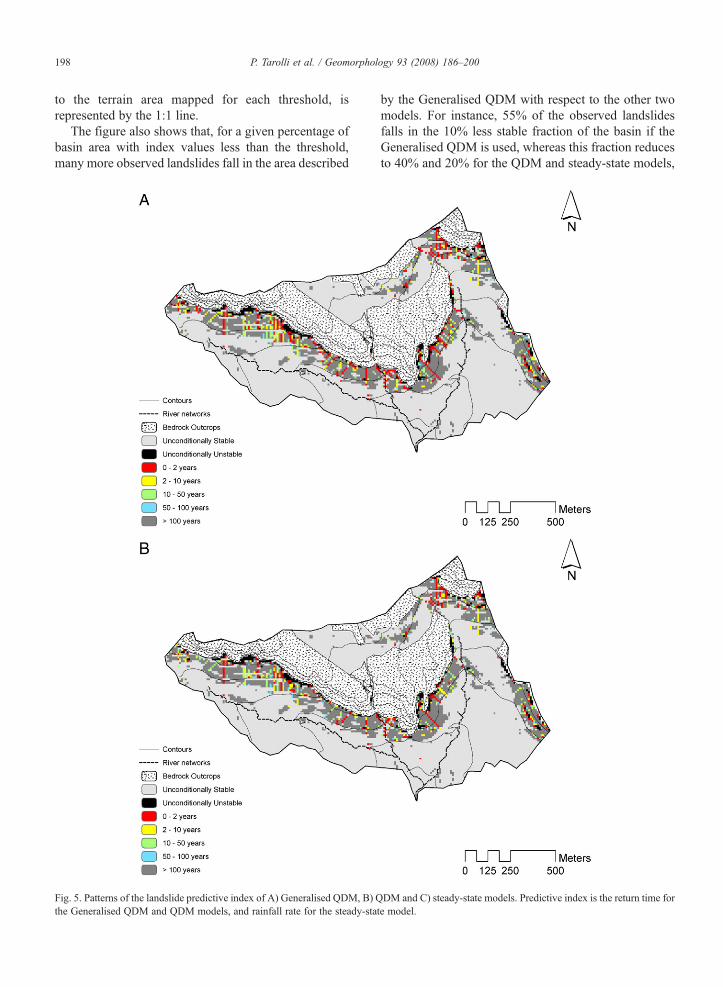
Maps of return time of critical rainfall are provided inFig. 5A,B for the Generalised QDM and the QDM,respectively, whereas Fig. 5C provides a map of criticalrainfall predicted from the steady-state model ofMontgomery and Dietrich (1994) using the same modelparameter set as used for the other two models. Asexpected, the Generalised QDM result differs from theQDM result only in the soil-mantled cells located onscrees close to rock walls. In this area, the GeneralisedQDM pattern is characterised by a greater frequency ofcells marked with low return time values than the QDMpattern.

Comparison with the pattern provided by the steady-state model is not feasible, since the model results arepresented in different ways. At each terrain element,the answer from the Generalised QDM and the QDM isa return period, whereas that from the steady-state

Table 4Percentages of slope-stability categories in terms of catchment areaand observed landslide area in each range of critical rainfall frequency(return time) for the QDM application

Frequency ofcritical rainfall(return time)

QD model



1.94 20.97

0–2 years 2.26 23.392–10 years 1.59 7.2610–50 years 1.48 6.4550–100 years 0.70 2.42N100 years 23.12 29.03Unconditionally

stable68.90 10.48

model is a critical rainfall. We adopted the approachdeveloped by Borga et al. (2002a) for their comparison,based on the proportion of catchment area which fallsbeneath a threshold of the instability-predictingvariable to the corresponding fraction of the landslidearea. First, a threshold needs to be set so that the samepercentage of terrain elements falls below it. Theunstable regions mapped from the application of themodels will be partially overlapping, but will not be thesame. Then the percentage of observed landslide areawithin the region is computed for each model. Themodel with the higher percentage is assumed to providea better prediction of landslide hazard. The assessmentmay be repeated for various thresholds. Note that themethodology implicitly assumes that the value of theindex variable decreases with increasing hazard, as it isfor the critical rainfall and the return time of the criticalrainfall.

The comparison was carried out in the following way.Let q be an index that is predictive of slope instability,which decreases with increasing hazard. The empiricaldistribution functions FB(q) and FL(q) are defined: FB

(q) represents the percentage of terrain elements with qless than the given value, and FL(q) represents thepercentage of landslide cells with q less than the givenvalue. A function is defined to express the relationshipbetween FL(q) and FB(q) for a given q-index model.Fig. 6 presents the functions for the Generalised QDM,QDM and steady-state models, where only the condi-tionally unstable fraction of the basin is considered. Inthe figure, better model performance would be reflectedin a convex curve, which indicates larger differencesbetween the fraction of catchment area and that ofobserved landslide area corresponding to low indexvalues. On the contrary, the ‘naive’ model, whichpredicts that slope instability occurs in direct proportion


to the terrain area mapped for each threshold, isrepresented by the 1:1 line.

The figure also shows that, for a given percentage ofbasin area with index values less than the threshold,many more observed landslides fall in the area described

Fig. 5. Patterns of the landslide predictive index of A) Generalised QDM, B) Qthe Generalised QDM and QDM models, and rainfall rate for the steady-sta

by the Generalised QDM with respect to the other twomodels. For instance, 55% of the observed landslidesfalls in the 10% less stable fraction of the basin if theGeneralised QDM is used, whereas this fraction reducesto 40% and 20% for the QDM and steady-state models,

DM and C) steady-state models. Predictive index is the return time forte model.

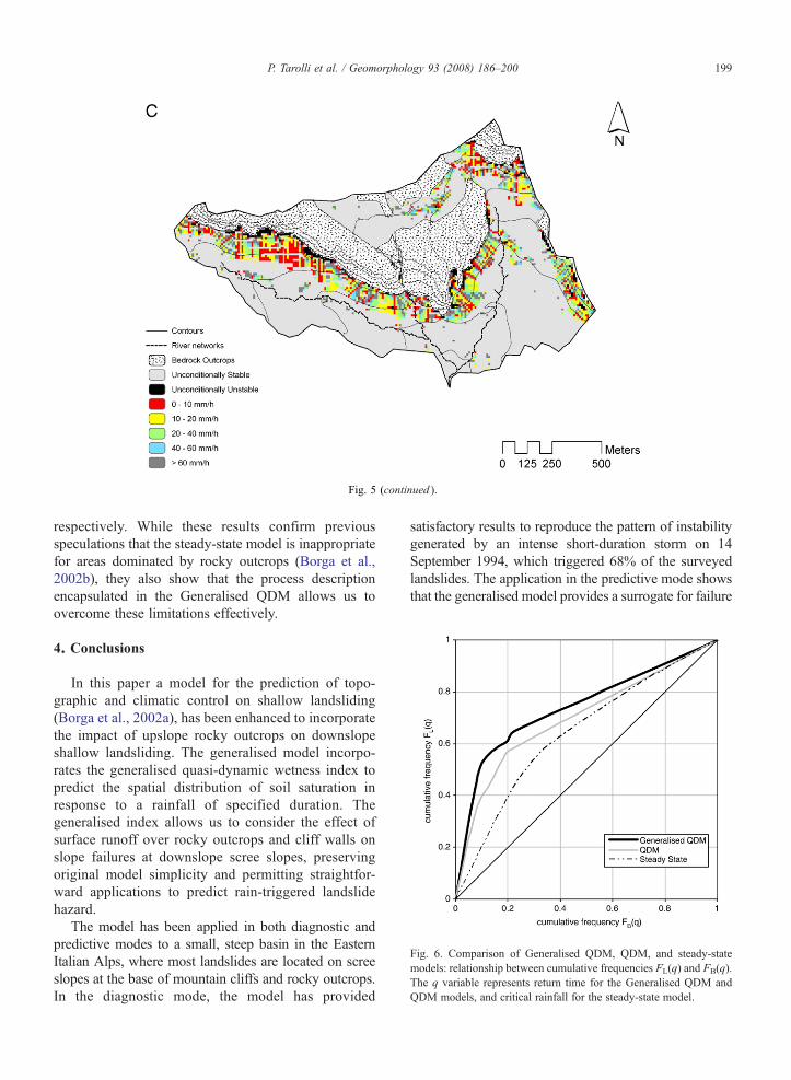
Fig. 5 (continued ).

Fig. 6. Comparison of Generalised QDM, QDM, and steady-statemodels: relationship between cumulative frequencies FL(q) and FB(q).The q variable represents return time for the Generalised QDM andQDM models, and critical rainfall for the steady-state model.


respectively. While these results confirm previousspeculations that the steady-state model is inappropriatefor areas dominated by rocky outcrops (Borga et al.,2002b), they also show that the process descriptionencapsulated in the Generalised QDM allows us toovercome these limitations effectively.

4. Conclusions

In this paper a model for the prediction of topo-graphic and climatic control on shallow landsliding(Borga et al., 2002a), has been enhanced to incorporatethe impact of upslope rocky outcrops on downslopeshallow landsliding. The generalised model incorpo-rates the generalised quasi-dynamic wetness index topredict the spatial distribution of soil saturation inresponse to a rainfall of specified duration. Thegeneralised index allows us to consider the effect ofsurface runoff over rocky outcrops and cliff walls onslope failures at downslope scree slopes, preservingoriginal model simplicity and permitting straightfor-ward applications to predict rain-triggered landslidehazard.

The model has been applied in both diagnostic andpredictive modes to a small, steep basin in the EasternItalian Alps, where most landslides are located on screeslopes at the base of mountain cliffs and rocky outcrops.In the diagnostic mode, the model has provided

satisfactory results to reproduce the pattern of instabilitygenerated by an intense short-duration storm on 14September 1994, which triggered 68% of the surveyedlandslides. The application in the predictive mode showsthat the generalised model provides a surrogate for failure


initiation probability as a function of hydrologicalconnectivity to rocky outcrops. Furthermore, a compar-ison with the quasi-dynamic (Borga et al., 2002a) andsteady-state (Montgomery and Dietrich, 1994) modelshas been carried out. The results suggest that the modelpresented here offers significant improvement over bothmodels, implying that the combination of the generalisedquasi-dynamic wetness index with the simple hydrolog-ical and slope-stability model provides an effective wayto describe the hyrological responses from rockyoutcrops.

Further research is needed (1) to evaluate the modelcapabilities and limitations in other rocky outcrop-dominated areas under different geographic conditions,(2) to assess model limitations associated with the presentsimplified approach based on a comparison with moredetailed hydrological and geomechanical models, (3) toevaluate the sensitivity of the model in relation to rainfallduration and antecedent soil moisture conditions, and(4) to evaluate the potential use of the model for analysingthe impact of increased impervious surfaces, followingurban development, on shallow landsliding.

Acknowledgements

The ARPAV—Centro Sperimentale Valanghe ofVeneto Region is acknowledged for the collaboration infield surveys. This work was supported by the EuropeanCommunity's Sixth Framework Programme, through thegrant to the budget of the Integrated Project FLOODsite,contract GOCE-CT-2004-505420 and by the Progetto diRicerca di Ateneo (University of Padova), CPDA052518.

References

Barling, D.B., Moore, I.D., Grayson, R.B., 1994. A quasi-dynamicwetness index for characterizing the spatial distribution of zones ofsurface saturation and soil water content. Water ResourcesResearch 30, 1029–1044.

Beven, K.J., 1981. Kinematic subsurface stormflow. Water ResourcesResearch 33, 1419–1424.

Beven, K.J., 1982a. On subsurface stormflow: predictions with simplekinematic theory for saturated and unsaturated flows. WaterResources Research 18, 1627–1633.

Beven, K.J., 1982b. On subsurface stormfow: an analysis of responsetimes. Hydrological Sciences Journal 4, 505–521.

Blijenberg, H.M., 1995. In-situ strength tests of coarse, cohesionlessdebris on scree slopes. Engineering Geology 39, 137–146.

Borga, M., Dalla Fontana, G., Da Ros, D., Marchi, L., 1998. Shallowlandslide hazard assessment using a physically based model anddigital elevation data. Environmental Geology 35, 81–88.

Borga,M., Dalla Fontana, G., Cazorzi, F., 2002a. Analysis of topographicand climatic control on rainfall-triggered shallow landsliding using aquasi-dynamic wetness index. Journal of Hydrology 268, 56–71.

Borga, M., Dalla Fontana, G., Gregoretti, C., Marchi, L., 2002b. Assess-ment of shallow landsliding by using a physically based model ofhillslope stability. Hydrological Processes 16, 2833–2851.

Borga, M., Dalla Fontana, G., Vezzani, C., 2005. Regional rainfalldepth-duration-frequency equations for an alpine region. NaturalHazards 36, 221–235.

Burlando, P., Rosso, R., 1996. Scaling and multiscaling models ofdepth-duration-frequency curves from storm precipitation. Journalof Hydrology 187, 45–64.

Carrara, A., Cardinali, M., Guzzetti, F., Reichenbach, P., 1995. GIStechnology in mapping landslide hazard. In: Carrara, A., Guzzetti,F. (Eds.), Geographical Information Systems in Assessing NaturalHazards. Kluwer Academic Publisher, Dordrecht, pp. 135–175.

Dunne, T., Black, R.D., 1970. An experimental investigation of runoffproduction in permeable soils.Water Resource Research 6, 478–490.

Folk, R.L., 1965. Petrology of Sedimentary Rocks. Univ. Texas,Hemphills Publ., Austin. 159 pp.

Glade, T., 2005. Linking debris-flow hazard assessments withgeomorphology. Geomorphology 66, 189–213.

Haeberli, W., Rickenmann, D., Zimmermann, M., 1990. Investigationof 1987 debris flows in the Swiss Alps: general concept andgeophysical soundings. IAHS Publication 194, 303–309.

Iida, T., 1999. A stochastic hydro-geomorphological model for shallowlandsliding due to rainstorm. Catena 34, 293–313.

Iverson, R.M., Reid, M.E., LaHusen, R.G., 1997. Debris-flowmobilization from landslides.AnnualReviews of Earth and PlanetarySciences 25, 85–138.

Lenzi, M., 2001. Step-pool evolution in the Rio Cordon, NortheasternItaly. Earth Surface Processes and Landforms Earth SurfaceProcess and Landforms 26, 991–1008.

Lenzi, M., Mao, L., Comiti, F., 2004. Magnitude-frequency analysis ofbed load data in an Alpine boulder bed stream. Water ResourcesResearch 40, W07201. doi:10.1029/2003WR002961.

Montgomery, D.R., Dietrich, W.E., 1994. A physically based modelfor the topographic control on shallow landsliding. WaterResources Research 30, 1153–1171.

Montgomery,D.R.,Dietrich,W.E., Torres, R.,Anderson, S.P.,Heffner, J.T.,Loague, K., 1997. Hydrologic response of a steep, unchanneled valleyto natural and applied rainfall. Water Resources Research 33, 91–109.

Reid, M.E., Iverson, R.M., 1992. Gravity-driven groundwater flowand landslide potential; 2, effects of slope morphology, materialproperties, and hydraulic heterogeneity. Water Resources Research28, 939–950.

Roering, J.J., Schmidt, K.M., Stock, J.D., Dietrich,W.E., Montgomery,D.R., 2003. Shallow landsliding, root reinforcement, and the spatialdistribution of trees in Oregon Coast Range. Canadian Geotech-nical Journal 40, 237–253.

Villi, V., Dal Prà, A., 2002.Debris flow in the upper Isarco valley, Italy—15 August 1998. Bulletin of Engineering Geology and the Envi-ronment 61, 49–57.

Wilkenson, F.D., Schmid, G.L., 2003. Debris flows in Glacier NationalPark, Montana: geomorphology and hazards. Geomorphology 55,317–328.

Wilson, C.J., Dietrich, W.E., 1987. The contribution of bedrockgroundwater flow to storm runoff and high pore pressure develop-ment in hollows. In: Beschta, R.L, Blinn, T., Grant, G.E., Ice, G.G.,Swanson, F.J. (Eds.), Erosion and Sedimentation in the Pacific Rim.International Association of Hydrological Sciences (IAHS) Publica-tion, vol. 165. IAHS Press, Wallingford, pp. 49–59.

http://dx.doi.org/10.1029/2003WR002961

Documents

Analysing the influence of upslope bedrock outcrops …intra.tesaf.unipd.it/people/tarolli/Papers/Tarolli et al. (2008).pdfAnalysing the influence of upslope bedrock outcrops on shallow