Analysing interactions of tted models - The · PDF fileThis vignette presents a brief review about the existing approaches for ... The post-hoc analysis of interactions in factorial

Analysing interactions of fitted models

Helios De Rosario Martınez

November 7, 2015

Abstract

This vignette presents a brief review about the existing approaches for the post-hoc analysis ofinteractions in factorial experiments, and describes how to perform some of the cited calculationsand tests with the functions of the package phia in R. Those functions include the calculation andplotting of cell means, and testing simple effects, residual effects, and interaction contrasts, amongother possibilities. They can be applied to linear and generalized linear models, with or withoutcovariates, and to mixed or multivariate linear models for repeated measures experiments.

1 Introduction

The post-hoc analysis of interactions in factorial ANOVA is a controversial issue, that has generatedmany discussions and a variety of methods. Traditionally, the most frequent practice has been theanalysis of simple main effects, i.e. the main effect of one factor at fixed values of the other factors.This type of analysis, however, has severly been criticized for its mixing both main and interactioneffects. Marascuilo and Levin stated in 1970 that analysing the simple effects of a significant interactionwas a typical case of the so-called “Type IV error”: a wrong interpretation of a correctly rejected nullhypothesis, since that analysis does not investigate the hypothesis that is presumably being tested [1].On the other hand, they proposed the analysis of interaction contrasts (crossed contrasts of differentfactors) or the interaction effects (the value of the interaction after removing low-order effects). Thelatter option was avidly supported by Rosnow and Rosenthal as well, who called that concept residualor leftover contrasts [2, 3].

However, such proposals have not produced an established “correct” practice at all. In fact, theanalysis of interactions has been a heated field of debate for years; see Games’ defence of simpleeffect tests [4] and Levin’s and Marascuilo’s response [5], or the criticisms of Meyer and Petty et al.to Rosnow’s and Rosenthal’s proposals [6, 7], as well as the answer to the latter [8]. Although thetheoretical issues of simple effects tests are generally acknowledged, an eventual consensus about the“best” alternative method is probably difficult to achieve. A general valid procedure is not possible inthe first place, since the correct test depends on the specific problem addressed by the experiment.

Unfortunately, many researchers do not choose a method depending on the question they want toanswer. In spite of the criticism received by the analysis of simple effects, various reviews of publishedresearch in the three last decades have shown that it still is by far the most frequent practice [2, 9, 10].According to Pardo’s et al. interpretation, this is partly due to the limitations of commonplace softwarepackages, which do not provide direct facilities for analysing the contrasts that isolate interaction effects[10].

On the other hand, the flexibility of R does allow to analyse any kind of contrast across the factorsof fitted models, even beyond the two- or three-factorial designs that are normally discussed in theliterature. After all, any contrast can be described as a linear combination of the model coefficients.Thus, since the mathematical details of fitted models (like their matrices of coefficients and covariances)are easily available in R, the values and errors of those contrasts can be calculated without difficulty, andmoreover there are contributed functions that facilitate the statistical tests based on such combinationsof coefficients, like linearHypothesis in the package car [11], or glht in multcomp [12], which isspecially suited for testing main effects.

1

The package phia (Post-Hoc Interaction Analysis) provides a usable interface for calculating dif-ferent types of contrasts, that are mentioned in the literature related to the analysis of interactions, aswell as other combinations of factors that could be of interest for the researcher. The functionality ofthis package also extends to more complex models, like generalized linear models, mixed-effects mod-els, multivariate linear models for repeated measures designs, and models with covariates. The testingprocedures provided by this package are the ones covered by linearHypothesis, i.e. tests based onF and χ2 statistics, with adjusted p-values if needed. The following sections of this paper give a moredetailed description of the main types of contrasts that can be used for analysing interactions, andexamples of using the functions of this package for calculating and testing them.

2 Mathematical formulation of interactions

Interactions are often described in terms of a linear, two-way factorial model, where the responsevariable Y is a function of the factors A and B. Interactions are said to exist when a change in thelevel of one factor has different effects on the response variable, depending on the value of the otherfactor [13]. This is often represented by the following formula:

Yijk = µ+ αi + βj + (αβ)ij + εijk, (1)

where αi, βj represent the “main effect” of the i-th and j-th levels of A and B, respectively, (αβ)ijis the effect of the interaction in that combination of levels, and εijk is the error term of the k-thobservation in that combination.

R analyses such models in the more general framework of linear models, defined by the followingmatrix equation:

Y(n×m)

= X(n×(r+1))

B((r+1)×m)

+ E(n×m)

, (2)

where Y contains the n observations of the m-dimensional response variable (with m often equal to1), X is the model matrix that only depends on the observed values of the predictor variables and thestructure of the model, B is the coefficient matrix for that model structure and data (with r degreesof freedom — d.o.f.), and E contains the error term.

The structure of X and B is very simple for linear regression models, where all predictors arenumeric variables. Let us take a regression model with an univariate response and two regressors (X1

and X2), including their interaction. In this case (2) would just be the formulation in matrix form ofthe regression equation: Y1

...Yn

=

1 X11 X21 X11X21

......

......

1 X1n X2n X1nX2n

β0β1β2β12

+

ε1...εn

(3)

This model has 3 terms, each with one d.o.f., that are represented by different columns of X andcoefficients of B (besides the intercept represented by the column of ones and β0). Two of these termsare the main effects of the regressors, represented by their values in X and the “slopes” β1, β2; theother one is the interaction term, represented by the product X1iX2i and the coefficient β12. For morecomplex regression models, there may be as many terms as possible products of regressors, such thatif there are k regressors, there may be up to k2 − 1 terms.

If some or all the predictor variables are factors, the same equations hold, but the representationof the terms in the model matrix would not be scalar values as X1i, X2i, or X1iX2i. The main termof each factor would be represented by a set of “dummy variables”, whose number would be equal tothe d.o.f. of the factor (the number of levels minus 1), and the interactions would be represented byall the possible products of the corresponding dummy variables. Thus, for instance, if there are twofactors A and B with 3 and 4 levels, respectively, the term of A would be represented by 2 dummyvariables, B by 3 of them, and their interaction by 2× 3 = 6 dummy variables.

2

The problem is that the coefficients that define the interactions in this framework are not alwaysuseful for describing the model in practical terms. The products of regressors are usually meaninglessvariables, and this poses a difficulty in the interpretation of the associated coefficients (see section 7below). This issue is further aggravated when there are factors involved in the interactions, since themeaning of the dummy variables may be even more opaque. That is one of the reasons that motivatethe different ways of describing interactions, which are commented on next.

3 Analysis of simple effects in factorial models

3.1 Calculation and plots of “cell means”

Let us take, for this and later sections, an example data set based on R.J. Boik’s hypothetical data [14],which he used for demonstrating how to analyse interaction contrasts in linear models, although it willbe used here for a larger variety of interaction analyses. It represents a hypothetical experiment, wherepeople affected by hemophobia were treated with different fear reduction therapies and different dosesof antianxiety medication, in a balanced factorial design, and the effect of these combined treatmentswas measured by their electrodermal response in an experimental session.

First we need to create the linear model from the data. We will use the data frame Boik also includedin the package phia, that has the response edr, and two factors (therapy, with levels control, T1, andT2; and medication, with levels placebo, D1, D2, and D3). We use the function some of the packagecar (imported by phia) to see some cases:

> library(phia)

> some(Boik)

therapy medication edr

5 control placebo 49.57396

13 control D2 47.64107

14 control D2 51.09978

19 control D3 42.47430

25 T1 placebo 50.90059

29 T1 placebo 50.66701

32 T1 D1 35.20488

40 T1 D2 29.37877

59 T2 D1 42.96335

61 T2 D2 36.03652

Before proceeding with detail analyses of the interactions, we should first check if the factorialmodel is coherent with the data, and if the interaction between both factors is actually significant. Wecan do this by examining the residuals of the model (see figure 1) and the ANOVA table.

> mod.boik <- lm(edr ~ therapy*medication, data=Boik)

> par(mfcol=c(1,2))

> plot(mod.boik, 1:2) # Plot diagnostics for the model

> Anova(mod.boik)

Anova Table (Type II tests)

Response: edr

Sum Sq Df F value Pr(>F)

therapy 2444.1 2 63.813 1.399e-15 ***

medication 2370.9 3 41.269 1.342e-14 ***

therapy:medication 1376.4 6 11.979 8.539e-09 ***

Residuals 1149.0 60

---

Signif. codes: 0 '***' 0.001 '**' 0.01 '*' 0.05 '.' 0.1 ' ' 1

3

20 30 40 50

−10

−5

05

10

Fitted values

Res

idua

ls●

●●

●

●

●

●

●

●

●

●

●

●

●

●

●

●

●

●

●

●

●

●

●

●

●●

●

●

●

●

●

●

●

●

●

●

●

●

●

●

●

●

●

●●

●

●

●

●

●

●

●

●

●

●

●

●

●

●●

●●

●

●

●

●

●

●

●

●

●

Residuals vs Fitted

1541

30

●

●●

●

●

●

●

●

●

●

●

●

●

●

●

●

●

●

●

●

●

●

●

●

●

●●

●

●

●

●

●

●

●

●

●

●

●

●

●

●

●

●

●

●

●

●

●

●

●

●

●

●

●

●

●

●

●

●

●●

●●

●

●

●

●

●

●

●

●

●

−2 −1 0 1 2

−3

−2

−1

01

2

Theoretical QuantilesS

tand

ardi

zed

resi

dual

s

Normal Q−Q

1541

30

Figure 1: Residuals vs. fitted values and Q-Q plot of mod.boik

Although the plots of figure 1 show a minor departure of normality for the residuals, specially dueto a couple of extremely low observations, for the sake of balance we will keep all data, and assumethat the model assumptions hold. Then we see in the ANOVA table that the interaction betweentherapy and medication is significant, so it does makes sense to investigate this effect.1

In factorial experiments like this one, the dependency between factor levels and the response variableis usually represented in a contingency table, where the rows and columns are related to the differentlevels of both treatments, and each cell contains the adjusted mean of the response for the correspondinginteraction of factors. When there is an interaction effect, the cell means are taken as the moststraightforward way of representing this effect. These values and their standard errors can be obtainedfrom the model coefficients with the function interactionMeans in the package phia, using the fittedmodel as first (and in this case only) argument:

> (boik.means <- interactionMeans(mod.boik))

therapy medication adjusted mean std. error

1 control placebo 50.20043 1.786533

2 T1 placebo 49.89963 1.786533

3 T2 placebo 45.69925 1.786533

4 control D1 47.49899 1.786533

5 T1 D1 38.20065 1.786533

6 T2 D1 39.09930 1.786533

7 control D2 45.99989 1.786533

8 T1 D2 28.50055 1.786533

9 T2 D2 36.50036 1.786533

10 control D3 47.89981 1.786533

1The data set is based on the results reported in Boik’s paper for the different tests, but not directly copied fromhis original work (that actually gives no data set). Thus, the residual plots are irrespective of Boik’s paper, and dueto rounding inaccuracies, the figures presented in this vignette and the ones of Boik’s tables differ in the last decimals.Regarding the ANOVA calculations, the Anova function from the package car has been used to be consistent with latersections, although for this set of balanced data the results would be the same if we had used anova from the base Rpackage.

4

2025

3035

4045

50 ●

●

●

●

●

therapy

controlT1T2

●

●●

control T1 T2

2025

3035

4045

50

placebo D1 D2 D3

●

medication

placeboD1D2D3

therapy medication

adjusted mean

Figure 2: Result of plot(boik.means)

11 T1 D3 18.99962 1.786533

12 T2 D3 32.69961 1.786533

This function calculates by default the cell means for the interactions of highest order betweenfactors. To obtain means of lower-order interactions, the optional argument factors admits a charactervector with the names of the factors that are included in the desired interaction.2 If this argumentgives only one factor, the result will be the means of its zeroth-order interaction (i.e. the marginalmeans for that factor). Thus, for instance:

> interactionMeans(mod.boik, factors="therapy")

therapy adjusted mean std. error

1 control 47.89978 0.8932665

2 T1 33.90011 0.8932665

3 T2 38.49963 0.8932665

The output of interactionMeans can be plotted via the generic plot method, that produces theset of plots shown in figure 2. The off-diagonal panels are the typical interaction plots, that can also becreated by interaction.plot from the columns of boik.means, where the lack of parallelism betweenlines reveals how one factor changes the effect of the other one. In this case, we see that the controlgroup hardly obtains any benefit from the medication, whereas with the other therapies (T1 and T2)the fear to blood is reduced proportionally to the medication dose, and more markedly for the former.On the other hand, the diagonal panels represent the marginal means of each factor.

If the interaction involved more than two factors, the graphical device would have as many rowsand columns as factors, and the off-diagonal panels would show the first-order interaction means foreach pair of factors. For interactions with many factors, the matrix of panels may be cluttered, so itwould be more convenient to show them in separate figures. The argument multiple (TRUE by default)can be modified for this purpose:

> plot(boik.means, multiple=FALSE) # Not printed in this paper

2But consider the contradiction of this approach with the marginality principle discussed in the next section.

5

3.2 Caveat : low-order interactions and the marginality principle

The basic methods of statistical analysis in R favour the so-called “marginality principle”, wherebythe main effects of factors with non-null interactions should not be interpreted or tested [15]. Now,the same warning applies to interactions that are themselves contained in interactions of higher order.Thus, although the plots described in the previous section are commonplace in the study of interactions,they are not necessarily meaningful in all circumstances.

For instance, since the interaction between therapy and medication is significant, according to themarginality principle we should not be concerned with the main effects of those factors, so the diagonalpanels of figure 2 would be irrelevant for this model. Likewise, if a model has more than two factors andan interaction of second or higher order is significant, no plot containing those factors would actuallybe of interest, since the method plot on the result of interactionMeans only represents main effectsand first-order interactions. (This is a limitation of the graphic representation alone, since the dataframe can represent higher-order interactions).

A suitable alternative for representing higher-order interactions are the functions effect andallEffects from the package effects [16]. Those functions are specially devised to analyse and plotthe interactions of highest order in the model. For factorial models, their outputs contain the same typeof data as interactionMeans, although they handle the numeric predictors of the model in anotherway, and the types of models that can be analysed is different (see sections 6 and 7).

3.3 Testing simple effects

The tabulation or graphical representation of cell means may give us a hint of the underlying structureof interactions, but they do not suffice to verify whether a specific change in the factors plays asignificant role in an interaction. As commented on above, the most frequent approach for solving thisissue consists in testing the simple effects, as an extension of the post-hoc methods that are widelyapplied to the study of main factor effects.

The available methods for the post-hoc analysis of main effects are manifold. The most basicprocedure consists in evaluating multiple contrasts between factor levels, possibly with corrections ofthe p-value in order to protect the family-wise error rate. Pairwise comparisons between levels areusually a default strategy when the researcher has no previous plan, although this is inefficient whenthe factor has many levels. Tukey’s method for testing pairwise contrasts, and Scheffe’s method forall possible contrasts within a factor, are probably the most popular ones. The package multcompprovides useful tools for this kind of main effects contrasts.

Testing simple main effects for interactions consists in evaluating contrasts across the levels of onefactor, when the values of the other interaction factors are fixed at certain levels. This test is thenrepeated at other fixed levels, and the results are compared. For instance, we could test the effect ofmedication at the different levels of therapy. This can be done with the function testInteractions,using the arguments fixed and across to define the factors that are fixed and tested across their levelsin each test:

> testInteractions(mod.boik, fixed="therapy", across="medication")

F Test:

P-value adjustment method: holm

medication1 medication2 medication3 Df Sum of Sq F Pr(>F)

control 2.3006 -0.4008 -1.8999 3 54.38 0.9465 0.4239

T1 30.9000 19.2010 9.5009 3 3153.95 54.8985 < 2.2e-16 ***

T2 12.9996 6.3997 3.8007 3 538.99 9.3818 7.117e-05 ***

Residuals 60 1149.01

---

Signif. codes: 0 '***' 0.001 '**' 0.01 '*' 0.05 '.' 0.1 ' ' 1

The columns medication1, . . . medication3 in the resulting table contain the value of the threeorthogonal contrasts across the levels of medication, for each level of therapy (the only fixed factor

6

in this example).3 The rest of columns show the information of the multivariate test applied to thosecontrasts. These tests just quantify the qualitative interpretation that was made from the plots: themedication does not have a significant effect for the control therapy group, but its effect is remarkablefor the other groups.

The criticism often posed to this method is that interactions are mixed with main effects (or lower-order interactions within), so the tests are not really related to the term that is supposedly underinvestigation. Using this example, the post-hoc analysis of the term therapy:medication is beingperformed because the ANOVA told us that it is significant; and this means that the coefficients ofthe matrix B related to this term are unlikely to be null. However, the tests of simple effects thathave just been described do not only involve those coefficients, but also the coefficients related to thelower-order terms therapy and medication.4

On the other hand, many researchers like simple effects for their relatively straightforward inter-pretation. Moreover, the interference of lower-order coefficients may be regarded a lesser issue whenthe marginality principle is considered. In this theoretical framework, the presence of a high-orderinteraction makes lower order terms meaningless, so that their effects are absorbed by the interaction.Therefore, the coefficients of lower order terms would partially be related to the interaction effect aswell.

4 Analysis of residual effects

To address the conceptual problems of simple effects, Rosnow and Rosenthal encouraged the analysisof residual effects, by “peeling away” the lower-order effects from cell means [2]. For instance, let ussee the cell means calculated in boik.means, in a table with the marginal means for both factors andthe grand mean:

> boik.mtable <- xtabs(boik.means$"adjusted mean" ~ therapy+medication, boik.means)

> boik.mtable <- addmargins(boik.mtable, FUN=mean, quiet=TRUE)

> print(boik.mtable, digits=4)

medication

therapy placebo D1 D2 D3 mean

control 50.2 47.5 46.0 47.9 47.9

T1 49.9 38.2 28.5 19.0 33.9

T2 45.7 39.1 36.5 32.7 38.5

mean 48.6 41.6 37.0 33.2 40.1

The “corrected means” would be obtained by subtracting the lowest-order effect (the grand mean)from the rest of values of the table, and then sweeping out the corrected marginal means from theindividual cells.

> boik.resid <- boik.mtable - boik.mtable[4,5] # Subtract the mean

> boik.resid <- sweep(boik.resid, 1, boik.resid[,5]) # Subtract row means

> boik.resid <- sweep(boik.resid, 2, boik.resid[4,]) # Subtract column means

> print(boik.resid, digits=4)

medication

therapy placebo D1 D2 D3 mean

control -6.1993 -1.9006 1.1997 6.9002 0.0000

T1 7.4996 2.8007 -2.3000 -8.0003 0.0000

T2 -1.3003 -0.9001 1.1003 1.1001 0.0000

mean 0.0000 0.0000 0.0000 0.0000 0.0000

3The specific contrasts that are calculated depend on various elements. In this case, since the original data framedefines medication as an ordered factor, polynomial contrasts are computed by default. For unordered factors they wouldhave been “sum-to-zero contrasts”. This default behaviour can be overriden by setting other contrast in the original dataframe, the fitted model, or with additional arguments in testInteractions.

4interactionTest does multiple calls to the function testFactors, which in its turn defines a linear combination ofthe model coefficients and passes it down to linearHypothesis from car. The hypothesis matrices used in these testscan be looked at to see what coefficients are actually involved.

7

1

1

1

1

−5

05

Inte

ract

ion

resi

dual

s

2

2

2

2

33

3 3

placebo D1 D2 D3

Figure 3: Residual effects of mod.boik

These values can also be calculated (and moreover tested) by testInteractions via the argumentresiduals, instead of fixed or across:

> testInteractions(mod.boik,residual=c("therapy","medication"))

F Test:


Value Df Sum of Sq F Pr(>F)

control (resid.) : placebo (resid.) -6.1993 1 461.17 24.0819 6.672e-05 ***

T1 (resid.) : placebo (resid.) 7.4996 1 674.93 35.2438 1.724e-06 ***

T2 (resid.) : placebo (resid.) -1.3003 1 20.29 1.0595 1.0000

control (resid.) : D1 (resid.) -1.9006 1 43.35 2.2635 0.8262

T1 (resid.) : D1 (resid.) 2.8007 1 94.13 4.9153 0.2434

T2 (resid.) : D1 (resid.) -0.9001 1 9.72 0.5077 1.0000

control (resid.) : D2 (resid.) 1.1997 1 17.27 0.9019 1.0000

T1 (resid.) : D2 (resid.) -2.3000 1 63.48 3.3148 0.5155

T2 (resid.) : D2 (resid.) 1.1003 1 14.53 0.7586 1.0000

control (resid.) : D3 (resid.) 6.9002 1 571.35 29.8353 9.515e-06 ***

T1 (resid.) : D3 (resid.) -8.0003 1 768.06 40.1073 4.069e-07 ***

T2 (resid.) : D3 (resid.) 1.1001 1 14.52 0.7584 1.0000


---

Signif. codes: 0 '***' 0.001 '**' 0.01 '*' 0.05 '.' 0.1 ' ' 1

However, these results may cause confusion, and their actual interest may be dubious in manycases, including the analysis of this model. We can plot the corrected means (ommiting the marginsof the table) for a clearer inspection of what is happening; see figure 3:

> matplot(t(boik.resid[-4,-5]), type="b", xaxt="n", ylab="Interaction residuals")

> axis(1, at=1:4, labels=levels(Boik$medication))

The lines of this plot (representing the three therapies) show the typical symmetry of residualeffects. The line labelled with 1 (the control group without specific therapy) shows a negative residual

8

effect of the placebo (a lower electrodermal response), that goes up to positive values as the medicationdose increases. The residual effects of the group treated with therapy T1 are the opposite, whereas thethe T2 group has a trend similar to the controls, but quite smaller.

The first problem is that a hasty interpretation of these values would lead to nonsense. Of course,they do not mean that the hemophobia of people that did not participate in any theraphy worsened withthe medication! The correct interpretation is that for these people, the effect of increasing medicationwas lower than value expected by the average of marginal means, and the opposite happened with thegroup treated with therapy T1.

But this reasoned interpretation, albeit mathematically sound, only has sense as long as the ex-pectations based on the marginal averages mean anything, and this is contrary to the principle ofmarginality commented on above. Since the factors therapy and medication do interact, the marginalmeans depend on the distribution of the sample across the factors; they are not reliable informationabout the response that we can expect for the different factor levels, except for a population with thesame distribution as the sample (in this case a balanced distribution). See, for instance, Games’ andMeyer’s discussion on this issue (although they do not explicitly refer to the “principle of marginality”)[4, 6].

That principle can be neglected if there is a good reason to study the marginal means that areobtained with a specific experimental design, but these circumstances are rare and special [17]. In thecurrent example there is no compelling reason to do so, therefore the significant differences found forthe placebo and the highest dose in different therapies are rather uninformative.

5 Interaction contrasts

Another alternative to simple effects is the study of interaction contrasts, which were in fact the subjectof the paper where our working data is derived from, although Boik used a slightly different procedurefor their analysis. Like in the analysis of interaction residuals, the hypothesis tested by interactioncontrasts is not affected by the coefficients of main effects, but this approach overcomes the commentedissue of interaction residuals, because it does not make use of marginal means, it only uses the dataof the cells [5, 6]. Interaction contrasts are defined as “differential effects”, or more descriptively as“differences of differences”, or “contrasts between contrasts”. They basically consist in calculatingone or more contrasts across a factor, and then iterating on the results of that operation across theremaining factors.

For instance, the test of simple effects previously calculated for mod.boik could be transformedinto a test of interaction contrasts, if instead of fixing the levels of therapy for evaluating the con-trasts across medication, we do pairwise contrasts between therapy levels. For this we must use theargument pairwise instead of fixed:

> testInteractions(mod.boik, pairwise="therapy", across="medication")

F Test:


medication1 medication2 medication3 Df Sum of Sq F Pr(>F)

control-T1 -28.599 -19.6019 -11.4008 3 1332.10 23.1869 1.302e-09 ***

control-T2 -10.699 -6.8005 -5.7007 3 175.95 3.0627 0.03481 *

T1-T2 17.900 12.8013 5.7002 3 556.55 9.6874 5.270e-05 ***


---

Signif. codes: 0 '***' 0.001 '**' 0.01 '*' 0.05 '.' 0.1 ' ' 1

These tests show how the contrasts across medication differ between pairs of therapy groups. Wecan see that the medication effect with the therapy T1 differs from the effect in controls and for theother therapy; the medication effect with T2 also differs from the effect in controls, but this variationis not so remarkable. This conclusion was not so clear from the simple effects tests. Moreover, theseresults are not disturbed by the main effects of factors at all, because the calculation of contrasts hasremoved them for both factors, without having defined them explicitly.

9

The most basic interaction contrasts involve pairwise contrasts for all factors. That is what testIn-teractions does by default, when only the model is specified.

> testInteractions(mod.boik)

F Test:



control-T1 : placebo-D1 -8.9975 1 121.43 6.3411 0.1448291


T1-T2 : placebo-D1 5.0990 1 39.00 2.0365 0.6951907

control-T1 : placebo-D2 -17.1985 1 443.68 23.1687 0.0001563 ***


T1-T2 : placebo-D2 12.2002 1 223.27 11.6587 0.0149653 *

control-T1 : placebo-D3 -28.5994 1 1226.89 64.0665 8.678e-10 ***

control-T2 : placebo-D3 -10.6990 1 171.70 8.9661 0.0439050 *

T1-T2 : placebo-D3 17.9004 1 480.63 25.0981 8.163e-05 ***

control-T1 : D1-D2 -8.2010 1 100.88 5.2681 0.2270868

control-T2 : D1-D2 -1.0999 1 1.81 0.0948 0.7592877

T1-T2 : D1-D2 7.1012 1 75.64 3.9498 0.4115755

control-T1 : D1-D3 -19.6019 1 576.35 30.0962 1.479e-05 ***

control-T2 : D1-D3 -6.8005 1 69.37 3.6224 0.4326396

T1-T2 : D1-D3 12.8013 1 245.81 12.8360 0.0095516 **

control-T1 : D2-D3 -11.4008 1 194.97 10.1810 0.0270962 *

control-T2 : D2-D3 -5.7007 1 48.75 2.5455 0.6951907

T1-T2 : D2-D3 5.7002 1 48.74 2.5450 0.6951907


---

Signif. codes: 0 '***' 0.001 '**' 0.01 '*' 0.05 '.' 0.1 ' ' 1

If all the factors of the model had 2 levels, this would have been an optimal strategy for analysingthe interaction, since the result would have been reduced to one test, corresponding to the single d.o.f.of such an interaction. But the factors with more levels heavily increase the number of tests, so thatfor our 3 × 4 factorial design, with 2 × 3 = 6 d.o.f., we obtain 18 overredundant tests. Such a highnumber of tests is difficult to interpret, let aside the lack of reliability of the p-values (with or withoutcorrections, that can be set by the argument adjustment in testInteractions).

A more sensible strategy consists in defining a small number of meaningful contrasts that can beof interest for the researcher. For instance, we might be interested in knowing the effect of crossingthe following contrasts for each factor

1. For therapy: controls vs. any therapy, and one therapy vs. the other.

2. For medication: placebo vs. any real dose, the minimum dose vs. the maximum, and themedium dose vs. the average of all doses.

The function testInteractions also allows to define such custom contrasts, via the argumentcustom. This argument must be a named list of matrices, one per factor, with the vectors of coefficientsthat define the contrasts arranged in columns. The auxiliary function contrastCoefficients providesa convenient interface to generate that list, from symbolic formulas that represent the contrasts:5

> (custom.contr <- contrastCoefficients(

+ therapy ~ control - (T1 + T2)/2, # Control vs. both therapies

+ therapy ~ T1 - T2, # Therapy T1 vs. T2

+ medication ~ placebo - (D1 + D2 + D3)/3, # Placebo vs. all doses

+ medication ~ D1 - D3, # Min. dose vs. max

+ medication ~ D2 - (D1 + D2 + D3)/3, # Med. dose vs. average

+ data=Boik, normalize=TRUE)) # Normalize to homogeinize the scale

5These matrices are transformed combinations of Helmert and polynomial contrasts, so they could have been definedby the functions contr.helmert and contr.poly as well.

10

$therapy

therapy therapy.1

control 0.8164966 0.0000000

T1 -0.4082483 0.7071068

T2 -0.4082483 -0.7071068

$medication

medication medication.1 medication.2

placebo 0.8660254 0.0000000 0.0000000

D1 -0.2886751 0.7071068 -0.4082483

D2 -0.2886751 0.0000000 0.8164966

D3 -0.2886751 -0.7071068 -0.4082483

Then use this list to define the contrasts in testInteractions (after renaming the columns of thematrices for a clearer interpretation of the output):

> names(custom.contr$therapy) <- c("cntrl.vs.all", "T1.vs.T2")

> names(custom.contr$medication) <- c("plcb.vs.all", "D1.vs.D3", "D2.vs.avg")

> testInteractions(mod.boik,custom=custom.contr)

F Test:



therapy : medication -8.7671 1 461.17 24.0819 4.448e-05 ***

therapy.1 : medication 7.1851 1 309.75 16.1749 0.0006558 ***

therapy : medication.1 -7.6217 1 348.54 18.2005 0.0003582 ***

therapy.1 : medication.1 6.4007 1 245.81 12.8360 0.0020468 **

therapy : medication.2 -1.3001 1 10.14 0.5296 0.9392219

therapy.1 : medication.2 -0.4044 1 0.98 0.0512 0.9392219


---

Signif. codes: 0 '***' 0.001 '**' 0.01 '*' 0.05 '.' 0.1 ' ' 1

This table of results is much clearer than the former. Moreover, all these contrasts are orthogonal toeach other (none of them can be obtained by combination of the others), so the tests are independent,and the adjustment of p-values is reliable. Taking some care about the meaning of positive and negativefigures of the Value column, we can obtain the following conclusions:

1. According to the first two tests, the benefit of taking medication (pooling over the three doses)is greater if the subject also receives some therapy, and this effect is specially marked for therapyT1.

2. And according to the second two tests, the therapies interact in the same manner with the benefitof increasing the medication from the minimum to the maximum. On the other hand, we cannotsay that the therapy influences the difference between the medium dose and the average of alldoses.

6 Multivariate models for repeated-measures

Repeated-measures experiments are common in many disciplines, including psychology and agriculture,although in the latter they are usually found with the specific strucutre and name of “split-plot”designs. The classical approach for analysing this kind of experiments is via multi-strata ANOVA orunivariate mixed-effects models, where the subjects or plots are introduced as factors with randomeffects, added to the error term (see section 9). However, when the design is balanced and adequatelysized, the multivariate approach is recommended if it possible, since it does not depend on the sphericityassumption and the results are more robust [18].

An example of such an analysis in R is published in the web appendices to Fox’s and Weisberg’sR Companion to Applied Regression [19]. We will use that example, based on the OBrienKaiser dataset from car [20].

11

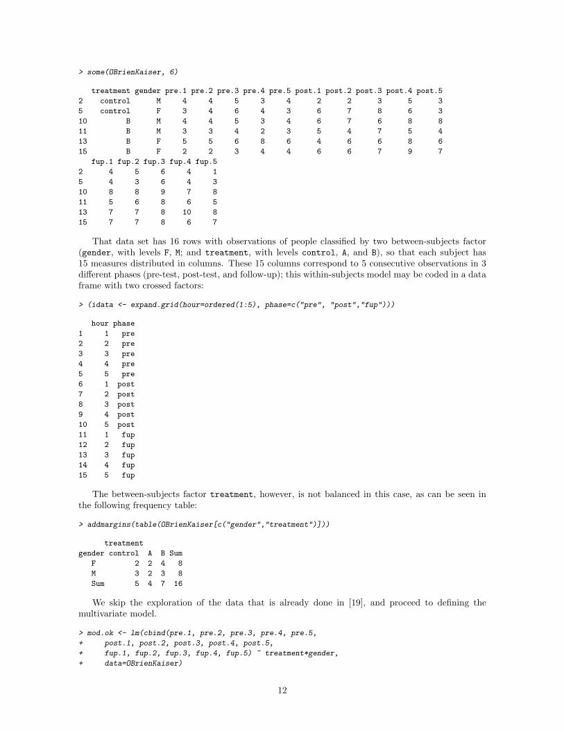
> some(OBrienKaiser, 6)

treatment gender pre.1 pre.2 pre.3 pre.4 pre.5 post.1 post.2 post.3 post.4 post.5

2 control M 4 4 5 3 4 2 2 3 5 3

5 control F 3 4 6 4 3 6 7 8 6 3

10 B M 4 4 5 3 4 6 7 6 8 8

11 B M 3 3 4 2 3 5 4 7 5 4

13 B F 5 5 6 8 6 4 6 6 8 6

15 B F 2 2 3 4 4 6 6 7 9 7

fup.1 fup.2 fup.3 fup.4 fup.5

2 4 5 6 4 1

5 4 3 6 4 3

10 8 8 9 7 8

11 5 6 8 6 5

13 7 7 8 10 8

15 7 7 8 6 7

That data set has 16 rows with observations of people classified by two between-subjects factor(gender, with levels F, M; and treatment, with levels control, A, and B), so that each subject has15 measures distributed in columns. These 15 columns correspond to 5 consecutive observations in 3different phases (pre-test, post-test, and follow-up); this within-subjects model may be coded in a dataframe with two crossed factors:

> (idata <- expand.grid(hour=ordered(1:5), phase=c("pre", "post","fup")))

hour phase

1 1 pre

2 2 pre

3 3 pre

4 4 pre

5 5 pre

6 1 post

7 2 post

8 3 post

9 4 post

10 5 post

11 1 fup

12 2 fup

13 3 fup

14 4 fup

15 5 fup

The between-subjects factor treatment, however, is not balanced in this case, as can be seen inthe following frequency table:

> addmargins(table(OBrienKaiser[c("gender","treatment")]))

treatment

gender control A B Sum

F 2 2 4 8

M 3 2 3 8

Sum 5 4 7 16

We skip the exploration of the data that is already done in [19], and proceed to defining themultivariate model.

> mod.ok <- lm(cbind(pre.1, pre.2, pre.3, pre.4, pre.5,

+ post.1, post.2, post.3, post.4, post.5,

+ fup.1, fup.2, fup.3, fup.4, fup.5) ~ treatment*gender,

+ data=OBrienKaiser)

12

The multivariate ANOVA with response transformation for repeated measures may be done withthe function Anova in car, using the auxiliary data frame idata, and the formula idesign with thewithin-subjects design. For the sake of coherence with the published example, we report a type-IIItest.

> Anova(mod.ok, idata=idata, idesign=~phase*hour, type=3)

Type III Repeated Measures MANOVA Tests: Pillai test statistic

Df test stat approx F num Df den Df Pr(>F)

(Intercept) 1 0.96736 296.389 1 10 9.241e-09 ***

treatment 2 0.44075 3.940 2 10 0.0547069 .

gender 1 0.26789 3.659 1 10 0.0848003 .

treatment:gender 2 0.36350 2.855 2 10 0.1044692

phase 1 0.81363 19.645 2 9 0.0005208 ***

treatment:phase 2 0.69621 2.670 4 20 0.0621085 .

gender:phase 1 0.06614 0.319 2 9 0.7349696

treatment:gender:phase 2 0.31060 0.919 4 20 0.4721498

hour 1 0.93286 24.315 4 7 0.0003345 ***

treatment:hour 2 0.31634 0.376 8 16 0.9183275

gender:hour 1 0.33922 0.898 4 7 0.5129764

treatment:gender:hour 2 0.57022 0.798 8 16 0.6131884

phase:hour 1 0.56043 0.478 8 3 0.8202673

treatment:phase:hour 2 0.66238 0.248 16 8 0.9915531

gender:phase:hour 1 0.71151 0.925 8 3 0.5894907

treatment:gender:phase:hour 2 0.79277 0.328 16 8 0.9723693

---

Signif. codes: 0 '***' 0.001 '**' 0.01 '*' 0.05 '.' 0.1 ' ' 1

Besides the intercept, the only significant effects at α = 0.05 are the main effects of phase andhour. Nevertheless, let us suppose that we have reasons to be more liberal, and want to investigatethe interaction treatment:phase that is near the α level of significance. (The main effect treatmentis also near that level, but we may ignore it since we will focus on its interaction with another factor).

The operations previously presented for univariate linear models can also be used in this case, asconvenient wrappers of the procedures recommended for the post-hoc analysis of multivariate models[21, 22].

First we may explore and plot the cell means of this interaction with interactionMeans, usingthe auxiliary data frame idata to specify the within-subjects model (idesign is not needed). We willuse the argument errorbar to draw the asymptotic 95% confidence intervals of the adjusted means,instead of their standard errors.6 The figure in the string "ci95" might be changed to calculate otherconfidence intervals, like "ci90", "ci99" for 90%, 99%, etc.

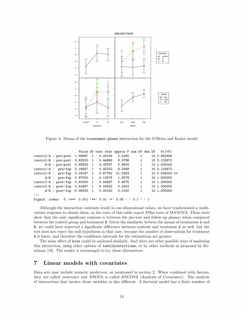
> ok.means <- interactionMeans(mod.ok, c("treatment","phase"), idata=idata)

> plot(ok.means, errorbar="ci95")

The plot of figure 4 shows that in the post-test and follow-up phases, the response of the controlgroup more or less remains at the same level as in the pre-test phase, whereas the response for theother treatments increases. However, the confidence intervals are relatively large, compared with thevariations between adjusted means, and there is a lot of overlap.

An analysis of all the possible interaction pairwise contratsts between treatment and phase helpus tell what differences are really significant:

> testInteractions(mod.ok, pairwise=c("treatment", "phase"), idata=idata)

Multivariate Test: Pillai test statistic


6These confidence intervals are not exact, but an approximation assuming that the parameters of the model arerandom results, normally distributed around their “true” values. This assumption is met asymptotically, if the samplesof data are large enough.

13

34

56

78

●

●

●

●

treatment

controlAB

●

●●

control A B

34

56

78

pre post fup

●

phase

prepostfup

treatment phase

adjusted mean

Figure 4: Means of the treatment:phase interaction for the O’Brien and Kaiser model

Value Df test stat approx F num Df den Df Pr(>F)

control-A : pre-post 1.66667 1 0.20106 2.5165 1 10 0.862456

control-B : pre-post 2.62500 1 0.44686 8.0786 1 10 0.132872

A-B : pre-post 0.95833 1 0.08787 0.9634 1 10 1.000000

control-A : pre-fup 2.16667 1 0.45202 8.2489 1 10 0.132872

control-B : pre-fup 3.04167 1 0.67782 21.0383 1 10 0.009002 **

A-B : pre-fup 0.87500 1 0.13478 1.5578 1 10 1.000000

control-A : post-fup 0.50000 1 0.04467 0.4675 1 10 1.000000

control-B : post-fup 0.41667 1 0.04032 0.4202 1 10 1.000000

A-B : post-fup -0.08333 1 0.00150 0.0150 1 10 1.000000

---

Signif. codes: 0 '***' 0.001 '**' 0.01 '*' 0.05 '.' 0.1 ' ' 1

Although the interaction contrasts result in one-dimensional values, we have trasformated a multi-variate response to obtain them, so the rows of this table report Pillai tests of MANOVA. These testsshow that the only significant contrast is between the pre-test and follow-up phases, when comparedbetween the control group and treatment B. Given the similarity betwen the means of treatments A andB, we could have expected a significant difference between controls and treatment A as well, but thetest does not reject the null hypothesis in that case, because the number of observations for treatmentA is lower, and therefore the confidence intervals for the estimations are greater.

The main effect of hour could be analysed similarly. And there are other possible ways of analysingthis interaction, using other options of testInteractions, or by other methods as proposed by Ke-selman [18]. The reader is encouraged to try these alternatives.

7 Linear models with covariates

Data sets may include numeric predictors, as mentioned in section 2. When combined with factors,they are called covariates and ANOVA is called ANCOVA (Analysis of Covariance). The analysisof interactions that involve these variables is also different. A factorial model has a finite number of

14

factor combinations where the adjusted mean of the response can be evaluated, but the possible valuesof a covariate are infinite. Therefore, the effects of covariates are usually represented as continuousfunctions within the range of their observed values (the model may allow the calculation of effectsbeyond that range, but such predictions would normally have little reliability).

We have seen that in factorial models, the effects of factors may be analysed by the contrastsbetween their levels. Obviously, the number of “contrasts” between possible values of a covariate wouldbe infinite, although they are constrained by the d.o.f. of the model. Let us take a pure linear regressionmodel without factors, and two covariates that do not interact:

Yi = β0 + β1X1i + β2X2i + εi (4)

For the effect of X1, there are infinite pairs of values X1a 6= X1b at which we could estimate such“contrasts”, but the expected value of the result would always be proportional to the difference betweenX1a and X1b. The ratio between both differences would be equal to the derivative of E (Y ) with respectto X1, which is equal to the model coefficient for X1:

∆E (Y )

∆X1=∂E (Y )

∂X1= β1 (5)

Thus, when covariates do not interact, their effects can just be described by the values of their cor-responding model coefficients. They are a measure of the “slope” along the covariate, or the incrementin the expected value of the response, when the covariate increases in one unit. Thus, if the researcheralso wants the adjusted value of the response for different values of the covariate, the only additionalinformation that he or she needs is the adjusted mean at an arbitrary point.

The functions of the package phia can report the values of those slopes. Let us take the model forthe prestige of Canadian occupations, defined in [11], p. 165. That model uses the data set Prestigefrom car, that contains several variables related to 102 different occupations:

> str(Prestige)

'data.frame': 102 obs. of 6 variables:

$ education: num 13.1 12.3 12.8 11.4 14.6 ...

$ income : int 12351 25879 9271 8865 8403 11030 8258 14163 11377 11023 ...

$ women : num 11.16 4.02 15.7 9.11 11.68 ...

$ prestige : num 68.8 69.1 63.4 56.8 73.5 77.6 72.6 78.1 73.1 68.8 ...

$ census : int 1113 1130 1171 1175 2111 2113 2133 2141 2143 2153 ...

$ type : Factor w/ 3 levels "bc","prof","wc": 2 2 2 2 2 2 2 2 2 2 ...

In this model, the prestige score of each profession (prestige) is fitted to a linear model thatdepends on education (average years of education), income (average income), and the factor type,that has three levels: bc (blue collar), prof (professional), and wc (white collar). The two formervariables are continuous covariates (income transformed to logarithmic scale to improve the normalityof the residuals), with different responses for the three types of ocupation (an interaction with type).We fit this model and do an ANOVA of it:

> mod.prestige <- lm(prestige ~ (log2(income)+education)*type, data=Prestige)

> Anova(mod.prestige)


Response: prestige


log2(income) 1690.8 1 41.1670 6.589e-09 ***

education 1209.3 1 29.4446 4.912e-07 ***

type 469.1 2 5.7103 0.004642 **

log2(income):type 290.3 2 3.5344 0.033338 *

education:type 178.8 2 2.1762 0.119474

Residuals 3655.4 89

---

Signif. codes: 0 '***' 0.001 '**' 0.01 '*' 0.05 '.' 0.1 ' ' 1

15

bc prof wc

46

810

12

type

log2(income)

Figure 5: Plot of the interaction log2(income):type

This analysis detects significant main effects of all the predictors, plus a significant interactionbetween log2(income) and the factor type. This interaction can explored with interactionMeans

(see figure 5) and tested with testInteractions, by just giving the name of the relevant covariate(s)in the argument slope. We also tell the name of the factor plotted at the X -axis and for which thepairwise contrasts are calculated (type), although it might be ommited in this case because there isno other factor in the model.

> plot(interactionMeans(mod.prestige, atx="type", slope="log2(income)"))

> testInteractions(mod.prestige, pairwise="type", slope="log2(income)")

Adjusted slope for log2(income)

F Test:



bc-prof 6.5356 1 256.2 6.2381 0.04302 *

bc-wc 5.6530 1 140.9 3.4311 0.13459

prof-wc -0.8825 1 3.3 0.0808 0.77684

Residuals 89 3655.4

---

Signif. codes: 0 '***' 0.001 '**' 0.01 '*' 0.05 '.' 0.1 ' ' 1

The plot and ANOVA table show the adjusted values of the slope with respect to log2(income)

(instead of the adjusted mean of the response), for the levels and contrasts of the factor type. Thatslope, i.e. the proportional relation between the occupation’s income and its prestige, is greater forblue collar occupations, whereas the difference is smaller between the other two types. However, thetests only reveal significant differences between blue collar and professionals, due to the unbalancednessof data. We can see in the ANOVA table that although the the adjusted slope of bc-prof is relativelysimilar to bc-wc, the sums of squares are far greater in the former case, since there are many morecases of prof:

> table(Prestige$type) # Frequencies of occupation types

16

bc prof wc

44 31 23

If there had been a significant interaction between the covariate education and type, we couldhave analysed it independently, since both covariates have an additive effect (they do not interact).Things may become more complicated if there are interactions between covariates. In that case, theslopes are not constant for given combinations of factors, but they are a function of the interactingcovariates. For instance, in a regression with two interacting variables:

Yi = β0 + β1X1i + β2X2i + β12X1X2 + εi, (6)

the slope with respect to X1 is (β1 + β12X2), and the slope for X2 is (β2 + β12X1).This means that the results of previous calculations may depend on the values of the other co-

variates. For instance, let us take another model for the Prestige data, where we consider thatlog2(income) and education can interact (the influence of the occupation’s income may vary withthe average years of education), and we discard the data of white collar occupations to have a morebalanced design and simpify things.

> mod.prestige2 <- update(mod.prestige, formula=.~.+(log2(income):education)*type,

+ subset=(Prestige$type!="wc"))

> Anova(mod.prestige2)


Response: prestige


log2(income) 1525.16 1 39.6299 2.702e-08 ***

education 719.35 1 18.6918 5.221e-05 ***

type 244.25 1 6.3466 0.01415 *

log2(income):type 194.83 1 5.0625 0.02774 *

education:type 3.80 1 0.0988 0.75424

log2(income):education 57.78 1 1.5013 0.22476

log2(income):education:type 3.30 1 0.0858 0.77048

Residuals 2578.49 67

---

Signif. codes: 0 '***' 0.001 '**' 0.01 '*' 0.05 '.' 0.1 ' ' 1

The significant effects shown by the ANOVA table are the same as for the previous model, includingthe interaction log2(income):type. And since type now has only two levels, the post-hoc test of thatinteraction gives virtually the same result as that table:

> testInteractions(mod.prestige2, pairwise="type", slope="log2(income)")


F Test:



bc-prof 12.721 1 194.19 5.0458 0.02799 *


---

Signif. codes: 0 '***' 0.001 '**' 0.01 '*' 0.05 '.' 0.1 ' ' 1

However, the algorithm used by this test (the function testFactors) sets the covariates at definitevalues, and the interaction between covariates considered by the model makes the test sensitive tothose values. The default values of the covariates are the averages of the cases observed in the modelfit. Nevertheless, the user may choose other arbitrary values, using the extra argument covariates

that is passed down to testFactors. This argument may contain a named numeric vector with thecustom values of any covariate. For instance, we might want to set education at its 75th quantile,and see what happens with the interaction log2(income):type.

17

> # Look quantiles of the model frame (a subset of the original data)

> quantile(model.frame(mod.prestige2)$education)

0% 25% 50% 75% 100%

6.380 8.015 9.930 13.990 15.970

> testInteractions(mod.prestige2, pairwise="type", slope="log2(income)",

+ covariates=c(education=14))


F Test:



bc-prof 10.862 1 62.02 1.6114 0.2087


Altering the value of education has substantially changed the result of the test on a term thatcontains log2(income), because of the interaction between both covariates. See, however, that thisinteraction, and other terms that contain it, are not significant according to the ANOVA of the model.So it could be wise to simplify the model (turning back to the original one), and remove this needlesslyproblematic interaction.

Now, if an interaction between covariates were really significant, the interest of the researcher shouldfocus on it. The high-order interactions in linear models have a constant effect at any combination ofthe covariates, so the problem of the arbitrary values used by the tests disappears. If the argumentslope of interactionMeans or testInteractions has the names of two or more covariates of themodel, the calculations will be done on the values of the coefficients related to those interactions (andhigher-order terms that might contain it). As commented on at the beginning of this document, thesecoefficients may be more difficult to understand, since the “slope” along a product of covariates mayseem meaningless, but it can just be interpreted as an extension of the analogy previously used betweenfactor contrasts and derivatives with respect to covariates.

We have already seen that when two factors interact, their effect can be evaluated by means of“contrasts between contrasts”. Likewise, when two covariates interact, we can study a “derivative ofthe derivative”, i.e. the second-order partial derivative of the response, which is represented by theinteraction coefficient. For the regression model of equation (6):

∂2E (Y )

∂X1∂X2= β12 (7)

This interpretation can be extended to third-order or higher interactions between covariates aswell, although models with that complexity are rarer, and the very meaning of such interactions willprobably more difficult to interpret than the coefficients used for representing them.

8 Generalized linear models

Generalized linear models (GLM) are very much like classical (Gaussian) linear models in most aspects,let aside the distribution of the error term and the expected value of the response, µ = E (Y ), that isrelated to the linear predictor by means of a link function η (µ). Accordingly, the interactions of suchmodels can be analysed by the methods explained in previous sections, although the interpretaton ofadjusted values in cell means and contrasts may be a bit more involved.

Let us take the example of the AMS survey about PhDs in mathematical sciences. This exampleuses the data set AMSsurvey of the package car, that contains a cross-classification of all the PhDsawarded in the mathematical sciences for different periods in US, assigned to 24 different categoriesdepending on various characteristics of the doctorate students [23].

> str(AMSsurvey)

18


$ type : Factor w/ 6 levels "I(Pr)","I(Pu)",..: 2 2 1 1 3 3 4 4 5 5 ...

$ sex : Factor w/ 2 levels "Female","Male": 2 1 2 1 2 1 2 1 2 1 ...

$ citizen: Factor w/ 2 levels "Non-US","US": 2 2 2 2 2 2 2 2 2 2 ...

$ count : int 132 35 87 20 96 47 47 32 71 54 ...

$ count11: int 148 40 63 22 161 53 71 28 89 55 ...

The data are structured in a data frame, with one row per category. The variable counts tells thenumber of PhDs of each category in 2008-2009, and the previous variables are factors that identifythe category.7 One of these factors is type, the type of institution the doctorate was affiliated with,and has 6 levels: I(Pr), I(Pu), II, III, IV, and Va; I to III are math departments in universities ofprogressively lower-quality — with pr ivate and public institutions distinguished by the parentheticalabbreviations, IV are statistics and biostatistics departments, and Va are applied mathematics depart-ments. The other factors are sex (the gender of the doctorate, a factor with levels Female and Male),and citizen (the citizenship status, a factor with levels Non-US and US). The contents of the dataframe are clearer if shown as a contingency table:

> ftable(xtabs(count ~ sex + citizen + type, AMSsurvey))

type I(Pr) I(Pu) II III IV Va

sex citizen

Female Non-US 25 29 50 39 105 12

US 20 35 47 32 54 14

Male Non-US 79 130 89 53 122 28

US 87 132 96 47 71 34

A saturated model of these data would represent count as a function of the three-way interactionof type, sex, and citizen. But the influences of sex and citizen are independent to each other, sowe can use a simplified model [11]. Since we are dealing with count data, the appropriate family wouldbe a Poisson distribution. All in all, the model could be defined as follows:

> mod.ams <- glm(count ~ type*(sex+citizen), family=poisson, data=AMSsurvey)

The ANOVA of this model confirms that the high-order interaction terms that remain are signifi-cant:

> Anova(mod.ams)

Analysis of Deviance Table (Type II tests)

Response: count

LR Chisq Df Pr(>Chisq)

type 233.336 5 < 2.2e-16 ***

sex 182.983 1 < 2.2e-16 ***

citizen 5.923 1 0.01494 *

type:sex 71.169 5 5.851e-14 ***

type:citizen 26.075 5 8.628e-05 ***

---

Signif. codes: 0 '***' 0.001 '**' 0.01 '*' 0.05 '.' 0.1 ' ' 1

The terms of interest are the interactions of type with sex and citizen. We may have a look onthe adjusted means with interactionMeans, as in other models. We tell that we want type in theX -axis, and the other factors coded as lines, with the arguments atx and traces, respectively:

> ams.means <- interactionMeans(mod.ams)

> plot(ams.means, atx="type", traces=c("sex","citizen"))

19

●

●

●

●

●

●

2040

6080

120

●

sex

FemaleMale

●

● ●

●

●

●

I(Pr) I(Pu) II III IV Va

2040

6080

120

●

citizen

Non−USUS

type

adjusted mean

Figure 6: Adjusted (geometric) means of the interactions in mod.ams

The resulting plots (see figure 6) are very similar to the ones shown in previous section, withthe exception of the Y -axis scale, which is nonlinear in this case. The reason is that for GLM,interactionMeans does not average over values of the response variable (the counts of awarded PhDs);the calculations are actually done in the link function domain, and the plots are drawn in its scale,although the resulting averages and the Y -axis labels are eventually transformed to show values of theresponse. In this case the link function is η = log (µ); therefore, the adjusted means are geometric (notarithmetic) means of the response variable,8 and the Y -axis is plotted in a logarithmic scale.

Nevertheless, the interpretation of the plot is not very affected by this issue. The mean number ofmale doctorates is higher in all institutions, but the difference seems larger in “first-class” universities(both public and private), and smaller in ‘third-class” universities or statistics departments (group IV).On the other hand, the influence of US-citizenship seems negligible except for statistics departments,where there are more foreign doctorates. The tables of testInteractions just confirm that thesedifferences are significant:

> testInteractions(mod.ams, pairwise=c("type","sex")) # test type:sex

Chisq Test:


Value Df Chisq Pr(>Chisq)

I(Pr)-I(Pu) : Female-Male 1.10975 1 0.2274 1.0000000

I(Pr)-II : Female-Male 0.51702 1 9.8992 0.0165352 *

I(Pr)-III : Female-Male 0.38181 1 17.7152 0.0003079 ***

I(Pr)-IV : Female-Male 0.32905 1 31.1081 3.417e-07 ***

I(Pr)-Va : Female-Male 0.64643 1 2.2978 0.6430680

I(Pu)-II : Female-Male 0.46588 1 16.5948 0.0005090 ***

I(Pu)-III : Female-Male 0.34405 1 26.1549 4.096e-06 ***

I(Pu)-IV : Female-Male 0.29651 1 47.8081 7.051e-11 ***

7AMSsurvey also contains data of other periods, but we will focus on the period 2008-2009. The analysis will be basedon a parsimonious model for those data, which is already fitted in [11, pp. 253–255].

8The adjusted link function is an arithmetic mean, but then: µ [∑

(ηi) /n] = exp [∑

(log µi) /n] =∏µ1/ni .

20

I(Pu)-Va : Female-Male 0.58250 1 3.9450 0.3290761

II-III : Female-Male 0.73848 1 2.3092 0.6430680

II-IV : Female-Male 0.63644 1 7.5105 0.0552052 .

II-Va : Female-Male 1.25031 1 0.7098 1.0000000

III-IV : Female-Male 0.86182 1 0.6219 1.0000000

III-Va : Female-Male 1.69308 1 3.5240 0.3629141

IV-Va : Female-Male 1.96453 1 6.9022 0.0688734 .

Residuals 6

---

Signif. codes: 0 '***' 0.001 '**' 0.01 '*' 0.05 '.' 0.1 ' ' 1

> testInteractions(mod.ams, pairwise=c("type","citizen")) #test type:citizen

Chisq Test:



I(Pr)-I(Pu) : Non-US-US 1.02087 1 0.0137 1.0000000

I(Pr)-II : Non-US-US 0.99993 1 0.0000 1.0000000

I(Pr)-III : Non-US-US 0.83462 1 0.7692 1.0000000

I(Pr)-IV : Non-US-US 0.53522 1 12.4565 0.0054149 **

I(Pr)-Va : Non-US-US 1.16636 1 0.3655 1.0000000

I(Pu)-II : Non-US-US 0.97949 1 0.0162 1.0000000

I(Pu)-III : Non-US-US 0.81756 1 1.1332 1.0000000

I(Pu)-IV : Non-US-US 0.52428 1 16.8929 0.0005932 ***

I(Pu)-Va : Non-US-US 1.14251 1 0.3055 1.0000000

II-III : Non-US-US 0.83468 1 0.8659 1.0000000

II-IV : Non-US-US 0.53526 1 14.6896 0.0017744 **

II-Va : Non-US-US 1.16643 1 0.3949 1.0000000

III-IV : Non-US-US 0.64128 1 5.4935 0.2099597

III-Va : Non-US-US 1.39747 1 1.6147 1.0000000

IV-Va : Non-US-US 2.17920 1 10.4188 0.0149688 *

Residuals 6

---

Signif. codes: 0 '***' 0.001 '**' 0.01 '*' 0.05 '.' 0.1 ' ' 1

Notice, however, that the interpretation of the column Value in these tables requires consideringthe relation between the link function and the response variable. We have combined pairwise contrasts,that result in differences in the domain of the link function; for instance if we focus on the interactioncontrast I(Pu)-II : Female-Male, the adjusted value of the link is:(

ηI(Pu),F − ηI(Pu)M

)− (ηII,F − ηII,M ) (8)

But ηi,j = log (µi,j), therefore the previous equation is equivalent to:

log

(µI(Pu),F

µI(Pu),M÷ µII,F

µII,M

)(9)

And if we go back to the response variable domain, the logarithm is cancelled, so we get that theinteraction contrasts is, in this case, a “ratio of ratios”, rather than a “difference of differences”. Inother words, the figure 0.47 in the column Value for the mentioned interaction contrast means thatthe proportion of females vs. males in “first-class” public universities is 0.47 times (less than half) theproportion in “second-class” universities. For other families of GLM, the interpretation of the contrastsin the domain of the response variable may be more obscure; so if desired, the argument link=TRUE

may be used in all the functions of phia to force the representation of the adjusted values in thedomain of the link function.

GLM may include covariates, and the analysis of interactions may involve terms that contain them.In that case, the means and contrasts reported by interactionMeans or testInteractions are alwaysin the link function domain, since the response variable keeps no linear relation with the predictors at

21

all, and therefore there is no such thing as “slopes” of that variable, except in very local, differentialenvironments.

Anyway, if there is some reason to do it, it is possible to obtain the derivatives of the responsevariable with respect to the covariates, via the “chain rule”. The slopes reported by the functions ofphia are derivatives of the link function, ∂η/∂Xi, and if model is the name of the object with thefitted GLM, we can obtain the derivative of the expected response with respect to the link, dµ/dη, asa function:

> dm.de <- family(model)$mu.eta

Now, to get the derivative of µ with respect to the covariate Xi at a specific value X, we just haveto evaluate de.dm at that value — type eval(dm.de(X)), with the desired value bound to X —, andthen mutliply:

∂µ

∂Xi(X) =

∂η

∂Xi

dµ

dη(X) (10)

More generally, all the calculations that may be done with classical linear models can also be appliedto GLM, but it is necessary to consider that the model is defined in terms of the link function, whereasthe outcomes are usually reported in units the response variable, and the calculations must be definedaccording to the domain where they operate.

9 Mixed-effects models

9.1 Differences with fixed-effects models

Linear and generalized linear models assume error independency between observations, i.e. that thereis no correlation between the values of the residual error. However, this assumption may be violated inmany experiments, where the observations are clustered in groups associated to noise factors, e.g. setsof measures taken in different environments, with different instruments, or in different subjects. Suchfactors are normally uninteresting for the purposes of the study, but their influence may nontheless besignificant. This conflict is solved by including the influence of those factors in the model, so that (2)is expanded as follows (simplifying the model to an univariate response):

Y(n×1)

= X(n×(r+1))

β((r+1)×1)

+ Z(n×s)

u(s×1)

+ ε(n×1)

, (11)

where the additional coefficients u and their corresponding model matrix Z are related to the s groupsof observations associated to the noise factors (plus their possible interctions with other factors andcovariates).

Now, if it is possible to assume that the effects of the noise factors (i.e. the coefficients representedin u) are random values from a normal distribution, the model may be simplified, so that instead offitting the individual values of u, it is only necessary to fit their covariance matrix Ψ, that is usuallyconstrained as a function of one or a few parameters. This is what is known as a mixed-effects model(with a combination of both “fixed” and “random” effects).9 These models may be analysed in R withthe functions included in the packages nlme [24] and lme4 [25]. In the following examples we will usethe latter, which is more flexible and efficient, although the procedure for analysing interactions is thesame in both cases.

The functions of phia for the post-hoc analysis of mixed-effects models are used just like in thecase of linear and generalized linear models. Multivariate responses in mixed-effects models are notsupported, however, although in some cases this may be worked around by a modification of the data

9The structure of the random part of the model is similar to the error term. In fact, in the limit case where all thegroups of random factors only contain one observation, Z is equivalent to the identity matrix, and the coefficients ucannot be distinguished from the residual errors ε. Obviously, in that case no special technique would be necessary forfitting the model, and the linear regression method would just do the work (although with an increased residual error).It is also possible to work with generalized mixed-effects models, where both the coefficients of random effects and theresidual error follow a non-normal distribution.

22

structure, as will be shown in the examples. From a theoretical point of view, another difference isthat the tests are not exact, so there may be concerns about the reliability of the reported p-values,as will be discussed in the examples as well.

Note, moreover, that the analysis is limited to the fixed effects, for good reasons. Random effectsare normally noise that must be controlled, but are not interesting for the conclusions of the study,and that is in fact why their effect is generally simplified as a set of random values. Accordingly, theparameters that are fitted in the model are not the specific values of the random effects, but theircovariances or other parameters that define their distribution. In other words: the model does notreally tell anything of those specific values, so we should not interrogate it about them.

Although the level of abstraction needed to understand this principle may be high in a complexmodel, it may be better grasped in a trivial model, defined just as the average of a set of randomvalues, plus the variance of the residual error. Doing a post-hoc about a random effect in a mixed-effects model is like asking in this case if two arbitrary observations are too far apart. This may be alegitimate diagnostic question at best, but a positive answer would just mean that the chosen modelis inadequate for those data.

9.2 Fitting and analysing a mixed-effects model

As an example to illustrate the post-hoc analysis of mixed-effects models, we will use Snijders’ andBosker’s data with language achievements of 2287 high-school students [26], included in the packagenlme. Following one of the examples worked by Snijders and Bosker, we will study the scores of alanguage test as a regression of the students’ IQ in verbal tasks and their socio-economical status (SES),possibly influenced by their gender, and the average SES and IQ of their schoolmates. In addition, wewill explore the strategy to analyse repeated-measures with a mixed-effects model, by comparing theachievements in two repetitions of the language test: at the start and end of the school year. All inall, the variables of interest in the original data frame bdf are:

langPRET: Score in the first repetition of the test.

langPRET: Score in the second repetition of the test.

pupilNR: Student code.

IQ.ver.cen: Student IQ (school-centered).

ses: Student socio-economical status (SES).

sex: Student gender.

schoolNR: School code.

schoolSES: School average SES

avg.IQ.ver.cen: School average IQ.

We first create a subset of the data frame with those variables, taken from the namespace of nlmewithout attaching it (with the operator ::).10 We will also add meaningful labels to the sex factor,and simplify some variable names for the sake of clarity.

> Snijders <- nlme::bdf[c("langPRET","langPOST", # Outcomes

+ "pupilNR", "IQ.ver.cen", "ses", "sex", # Student-related variables

+ "schoolNR", "schoolSES", "avg.IQ.ver.cen")] # School-related variables

> Snijders$sex <- factor(Snijders$sex, labels=c("F","M"))

> names(Snijders) <-

+ c("score.1","score.2","student","IQ","SES","sex","school","avgSES","avgIQ")

10Since the namespaces of nlme and lme4 partially overlap, it is not advisable to load both packages in the samesession.

23

Following Snijders and Bosker, for a better model fit we will also include quadratic components ofIQ around 0 (remember that the IQ variable is centered) [26, p. 113].

> Snijders$IQ2.pos <- with(Snijders, (IQ > 0)*IQ^2)

> Snijders$IQ2.neg <- with(Snijders, (IQ < 0)*IQ^2)

The model proposed by Snijders and Bosker was focused on the result of one of the tests (sayscore.2, and contained the following fixed terms: the crossed linear effect of IQ and SES, both atstudent level (IQ*ses) and at school level (avgIQ*avgSES), the quadratic effects of IQ (IQ2.pos,IQ2.neg), and the effect of gender (sex). They also considered that the average scores and the lineareffect of IQ could be grouped by school. Such a model could be fitted as follows:

> library(lme4)

> form1 <- score.2 ~

+ IQ * SES + IQ2.pos + IQ2.neg + sex + avgIQ * avgSES + # Fixed part

+ (IQ | school) # Random part

> mod.snijders.1 <- lmer(form1, data=Snijders)

Now, this is one of the cases where we cannot use the multivariate approach described in section 6for analysing the effect of repeating the test. We could attempt a similar analysis step-by-step, fittingtwo models with different dependent variables, corresponding to the response transformations that areused in the analysis of within-subjects effects. Both models would have the same right-hand side ofthe formula as form1 above. The dependent variable in one of them would be the average of score.1and score.2; in the other one it would be their difference:

> form2.1 <- update(form1, (score.1+score.2)/2~.)

> form2.2 <- update(form1, (score.2-score.1)~.)

If we consider that score.1 and score.2 are two subsets of the same variable, distinguished by atwo-level factor (say repetition), the model fitted with form2.1 would tell us the effects of the termsdefined in that formula on the pooled variable, whereas the model fitted with form2.2 would define theeffects of the interaction between repetition and those terms (i.e. repetition:IQ, repetition:SES,etc.).

On the other hand, we may fit a single model that accounts for all the terms that we want toanalyse with more flexibility. For that, we first have to transform the “wide” data frame with score.1

and score.2 as different columns, into a “long” data frame with both of them in one column. We willalso need the repetition factor explicitly defined in the data frame, and a variable that identifieseach original row (the already existing variable student in the original frame can do that work). Wecan get all this with the reshape function:

> Snijders.long <- reshape(Snijders, direction="long", idvar="student",

+ varying=list(c("score.1","score.2")), v.names="score", timevar="repetition")

> # The within-subjects factor must be coded as a factor

> Snijders.long$repetition <- as.factor(Snijders.long$repetition)

> # See the variables of the long data frame

> str(Snijders.long)


$ student : Factor w/ 2287 levels "17001","17002",..: 1 2 3 4 5 6 7 8 9 10 ...

$ IQ : num 3.166 2.666 -2.334 -0.834 -3.834 ...

$ SES : num 23 10 15 23 10 10 23 10 13 15 ...

$ sex : Factor w/ 2 levels "F","M": 1 1 1 1 1 1 1 1 1 1 ...

$ school : Ord.factor w/ 131 levels "47"<"103"<"2"<..: 119 119 119 119 119 119 119 119 119 119 ...

$ avgSES : num 11 11 11 11 11 11 11 11 11 11 ...

$ avgIQ : Named num -1.51 -1.51 -1.51 -1.51 -1.51 ...

..- attr(*, "names")= chr "1" "1" "1" "1" ...

$ IQ2.pos : num 10.02 7.11 0 0 0 ...

24

$ IQ2.neg : num 0 0 5.448 0.696 14.7 ...

$ repetition: Factor w/ 2 levels "1","2": 1 1 1 1 1 1 1 1 1 1 ...

$ score : num 36 36 33 29 19 22 20 44 34 31 ...

- attr(*, "reshapeLong")=List of 4

..$ varying:List of 1

.. ..$ : chr "score.1" "score.2"

..$ v.names: chr "score"

..$ idvar : chr "student"

..$ timevar: chr "repetition"

Now we can use this data frame to fit a model based on the formula form1, adding the interactionsof repetition with the terms we want (in the multivariate approach, all the interactions of between-subjects and within-subjects terms are always included). The price that is paid for that is the additionof the random effects of student, since now we have more than one observation for each value of thisfactor.

We will consider that the repetition only interacts with the student-related terms. Regarding therandom effects, the student factor can only influence the intercept term, since all the other terms ofthe model are constant for the two measures of each student. Thus, the new formula and the modelfitted with it will be:

> form3 <- score ~

+ repetition * (IQ * SES + IQ2.pos + IQ2.neg + sex) + # Student-related

+ avgIQ * avgSES + # School-related

+ (IQ | school) + (1 | student) # Random part

> mod.snijders.3 <- lmer(form3, data=Snijders.long)

> # See the main parameters of the model (ommit correlations table)

> print(mod.snijders.3, correlation=FALSE)

Linear mixed model fit by REML ['lmerMod']

Formula: score ~ repetition * (IQ * SES + IQ2.pos + IQ2.neg + sex) + avgIQ *

avgSES + (IQ | school) + (1 | student)

Data: Snijders.long

REML criterion at convergence: 28555.76

Random effects:

Groups Name Std.Dev. Corr

student (Intercept) 3.7060

school (Intercept) 1.8851

IQ 0.2058 -1.00

Residual 4.2474

Number of obs: 4574, groups: student, 2287; school, 131

Fixed Effects:

(Intercept) repetition2 IQ SES

31.85442 4.27322 2.65186 0.09074

IQ2.pos IQ2.neg sexM avgIQ

-0.13133 0.14604 1.23928 1.64627

avgSES IQ:SES repetition2:IQ repetition2:SES

-0.04053 -0.01403 1.41339 0.06727

repetition2:IQ2.pos repetition2:IQ2.neg repetition2:sexM avgIQ:avgSES

-0.17917 0.16430 1.39074 -0.04550

repetition2:IQ:SES

-0.01065

As said above, the methods for analysing a model like this are similar to the ones used in fixed-effectsmodels. However, there are important caveats about the results that must be considered.

The main objective of many researchers in their using statistical techniques for data analysis is toobtain p-values to accept or reject their hypothesis, but the calculation of those values in mixed-effectsmodels is problematic. That is the reason why the table of coefficients of a model fitted by lmer does

25

not show p-values, as may be seen above, nor are they presented in the ANOVA table given by thestandard anova method [27].11

There are different techniques for working around this problem, like the Kenward-Roger approxi-mation or parametric bootstrap, which are implemented in the package pbkrtest [28]. An alternativeapproach is assuming that the covariances of the random part of the model are equal to the estimatedvalues, and then use standard tests [29]. The function Anova from car produces tables with p-valuesbased on Wald tests, following the latter assumption [30], and by extension, the same happens withthe test functions of the package phia, which are also dependent on the function linearHypohtesis

from car.This being said, we can first look what terms are significant according to the Wald tests:

> Anova(mod.snijders.3)

Analysis of Deviance Table (Type II Wald chisquare tests)

Response: score

Chisq Df Pr(>Chisq)

repetition 2882.6797 1 < 2.2e-16 ***

IQ 479.2605 1 < 2.2e-16 ***

SES 110.2884 1 < 2.2e-16 ***

IQ2.pos 30.8978 1 2.720e-08 ***

IQ2.neg 45.3553 1 1.643e-11 ***

sex 89.5824 1 < 2.2e-16 ***

avgIQ 12.0599 1 0.0005152 ***

avgSES 0.9457 1 0.3308162

IQ:SES 13.7841 1 0.0002051 ***

repetition:IQ 52.3654 1 4.608e-13 ***

repetition:SES 28.8549 1 7.801e-08 ***

repetition:IQ2.pos 13.4414 1 0.0002461 ***

repetition:IQ2.neg 16.3300 1 5.321e-05 ***

repetition:sex 30.4621 1 3.405e-08 ***

avgIQ:avgSES 1.1707 1 0.2792546

repetition:IQ:SES 2.9505 1 0.0858501 .

---

Signif. codes: 0 '***' 0.001 '**' 0.01 '*' 0.05 '.' 0.1 ' ' 1

The ANOVA table shows that most terms of our model are significant for the Wald test at α = 0.05.The exceptions are the terms related to avgSES, and the second-order interaction of repetition withIQ and SES.

All the remaining main and interaction effects of factors and covariates could further be investigated,as explained in the previous sections. Just as an example, let us focus on the only interaction betweenfactors: repetition:sex. We can see the table of average scores, and calculate the simple main effectsand pairwise interactions:

> # Cell means

> interactionMeans(mod.snijders.3)

repetition sex adjusted mean SE of link

1 1 F 33.67415 0.2501164

2 2 F 39.82938 0.2501164

3 1 M 34.91343 0.2561410

4 2 M 42.45940 0.2561410

> # Simple effect of sex at each repetition

> testInteractions(mod.snijders.3, fixed="repetition", across="sex")

11Mixed models fitted with lme from the package nlme do show p-values, but this does not mean that they shouldalways be trusted.

26

Chisq Test:



1 -1.2393 1 26.638 2.454e-07 ***

2 -2.6300 1 119.973 < 2.2e-16 ***

---

Signif. codes: 0 '***' 0.001 '**' 0.01 '*' 0.05 '.' 0.1 ' ' 1

> # Pairwise interactions (default)

> testInteractions(mod.snijders.3)

Chisq Test:



1-2 : F-M 1.3907 1 30.462 3.405e-08 ***

---

Signif. codes: 0 '***' 0.001 '**' 0.01 '*' 0.05 '.' 0.1 ' ' 1

These results show that female students had significantly lower scores than boys, and that in thesecond repetition that difference was two times the initial one. Note, however, that the size of thedifference is small in spite of the statistical significance (gender differences were between 1 and 3 points,for scores that were normally over 30 points).

That is something that often happens when models are fitted to very large data bases, and thatreminds us that p-values must always be taken carefully and with a critical thought. In this case,where we used thousands of observations, we may suspect that many of the effects with low p-valuesin the ANOVA table may be irrelevant. In fact, if we look at the coefficients of the model (in the tableabove) and the ranges of the associated covariates in the data frame, we can see that most effects arenegligible in size when compared with the differences associated to repetition and the linear effectof IQ. This means that they are not relevant from a practical point of view, even though they maycontribute to a significantly better fit of the model.

Acknowledgements

I thank Professors John Fox and Michael Friendly, for their encouragement and advise in the creationof the functions of phia.

References

[1] L. A. Marascuilo and J. R. Levin, “Appropriate post hoc comparisons for interaction and nestedhypotheses in analysis of variance designs: The elimination of type IV errors,” American Educa-tional Research Journal, vol. 7, no. 3, pp. 397–421, 1970.

[2] R. L. Rosnow and R. Rosenthal, “Definition and interpretation of interaction effects,”PsychologicalBulletin, vol. 105, no. 1, pp. 143–146, 1989.

[3] R. L. Rosnow and R. Rosenthal, ““Some things you learn aren’t so”: Cohen’s paradox, Asch’sparadigm, and the interpretation of interaction,” Psychological Science, vol. 6, no. 1, pp. 3–9,1995.

[4] P. A. Games, “Type IV errors revisited.,” Psychological Bulletin, vol. 80, no. 4, pp. 304–307, 1973.

[5] J. R. Levin and L. A. Marascuilo, “Type IV errors and Games.,” Psychological Bulletin, vol. 80,no. 4, pp. 308–309, 1973.

[6] D. L. Meyer, “Misinterpretation of interaction effects: a reply to Rosnow and Rosenthal,” Psycho-logical Bulletin, vol. 110, no. 3, pp. 571–573; discussion 574–576, 1991.

27

[7] R. E. Petty, L. R. Fabrigar, D. T. Wegener, and J. R. Priester, “Understanding data when inter-actions are present or hypothesized,” Psychological Science, vol. 7, no. 4, pp. 247–252, 1996.

[8] R. L. Rosnow and R. Rosenthal,“Contrasts and interactions redux: Five easy pieces,”PsychologicalScience, vol. 7, no. 4, pp. 253–257, 1996.

[9] K. J. Ottenbacher, “Interpretation of interaction in factorial analysis of variance design,” Statisticsin Medicine, vol. 10, no. 10, pp. 1565–1571, 1991.

[10] A. Pardo, J. Garrido Garcıa, M. A. Ruiz, and R. San Martın Castellanos, “La interaccion entrefactores en el analisis de varianza: errores de interpretacion,” Psicothema, vol. 19, no. 2, pp. 343–349, 2007.

[11] J. Fox and S. Weisberg, An R Companion to Applied Regression. Thousand Oaks CA: Sage,second ed., 2011.

[12] T. Hothorn, F. Bretz, and P. Westfall, “Simultaneous inference in general parametric models,”Biometrical Journal, vol. 50, no. 3, pp. 346–363, 2008.

[13] Y. Dodge, The concise encyclopedia of statistics. Springer, 2008.

[14] R. J. Boik, “Interactions, partial interactions, and interaction contrasts in the analysis of vari-ance.,” Psychological Bulletin, vol. 86, no. 5, pp. 1084–1089, 1979.

[15] J. A. Nelder, “A reformulation of linear models,” Journal of the Royal Statistical Society. SeriesA (General), vol. 140, no. 1, pp. 48–77, 1977.

[16] J. Fox and J. Hong, “Effect displays in R for multinomial and proportional-odds logit models:Extensions to the effects package,” Journal of Statistical Software, vol. 32, pp. 1–24, 10 2009.

[17] W. Venables, “Exegeses on linear models.” Paper presented to the S-PLUS User’s Conference(Washington, DC, 8-9th October, 1998), 2000.

[18] H. J. Keselman, “Testing treatment effects in repeated measures designs: an update for psy-chophysiological researchers.,” Psychophysiology, vol. 35, no. 4, pp. 470–478, 1998.

[19] J. Fox and S. Weisberg, “Multivariate Linear Models in R. an appendix to An R Companion toApplied Regression, second edition,” July 2011.

[20] R. G. O’Brien and M. K. Kaiser, “MANOVA method for analyzing repeated measures designs: anextensive primer.,” Psychological Bulletin, vol. 97, no. 2, pp. 316–333, 1985.

[21] J. Fox, “Post-hoc after Anova() car package using linear.hypothesis() in a repeated measure anal-ysis.” R-help Archive, September 27 2007.

[22] J. Fox, “Multiple comparisons on anova.mlm object.” R-help Archive, April 17 2010.

[23] P. Phipps, J. W. Maxwell, and C. A. Rose, “2009 Annual Survey of the Mathematical Sciences inthe United States (first report),” Notices of the AMS, vol. 57, no. 2, pp. 250–259, 2010. Supple-mentary Table 4.

[24] J. Pinheiro, D. Bates, S. DebRoy, D. Sarkar, and R Core Team, nlme: Linear and NonlinearMixed Effects Models, 2015. R package version 3.1-122.

[25] D. Bates, M. Maechler, B. Bolker, and S. Walker, lme4: Linear mixed-effects models using Eigenand S4, 2015. R package version 1.1-9.

[26] T. A. B. Snijders and R. J. Bosker, Multilevel Analysis: An Introduction to Basic and AdvancedMultilevel Modeling. Sage, 1999.

[27] D. Bates, “lmer, p-values and all that.” R-help Archives, May 19 2006.

28

[28] U. Halekoh and S. Højsgaard, “A kenward-roger approximation and parametric bootstrap methodsfor tests in linear mixed models – the R package pbkrtest,” Journal of Statistical Software, vol. 59,no. 9, pp. 1–30, 2014.

[29] J. J. Faraway, Extending the Linear Model with R: generalized linear, mixed effects and non-parametric regression models. Boca Raton: Chapman & Hall / CRC, 2006.

[30] B. Bolker, “F and wald chi-square tests in mixed-effects models.” R-sig-ME Archives, October 42011.

29

Documents

Analysing interactions of tted models - The · PDF fileThis vignette presents a brief review about the existing approaches for ... The post-hoc analysis of interactions in factorial