ANALYSING AND COMPUTING TURBULENT FLOWS USING WAVELETS

“farge”2001/11/20page 450

�

�

�

�

�

�

�

�

COURSE 9

ANALYSING AND COMPUTINGTURBULENT FLOWSUSING WAVELETS

M. FARGE K. SCHNEIDER

LMD-CNRS,Ecole Normale Superieure,

24 rue Lhomond,75231 Paris Cedex 05, France

CMI,Universite de Provence,

39 rue Joliot–Curie,13453 Marseille Cedex 13, France

“farge”2001/11/20page 451

�

�

�

�

�

�

�

�

Contents

1 Introduction 453

I Wavelet Transforms 456

2 History 456

3 The continuous wavelet transform 457

3.1 One dimension . . . . . . . . . . . . . . . . . . . . . . . . . . . . . 457

3.2 Higher dimensions . . . . . . . . . . . . . . . . . . . . . . . . . . . 459

3.3 Algorithm . . . . . . . . . . . . . . . . . . . . . . . . . . . . . . . . 460

4 The orthogonal wavelet transform 461

4.1 One dimension . . . . . . . . . . . . . . . . . . . . . . . . . . . . . 461

4.2 Higher dimensions . . . . . . . . . . . . . . . . . . . . . . . . . . . 463

4.3 Algorithm . . . . . . . . . . . . . . . . . . . . . . . . . . . . . . . . 466

II Statistical Analysis 468

5 Classical tools 468

5.1 Methodology . . . . . . . . . . . . . . . . . . . . . . . . . . . . . . 468

5.2 Averaging procedure . . . . . . . . . . . . . . . . . . . . . . . . . . 469

5.3 Statistical diagnostics . . . . . . . . . . . . . . . . . . . . . . . . . 470

6 Statistical tools based on the continuous wavelet transform 473

6.1 Local and global wavelet spectra . . . . . . . . . . . . . . . . . . . 473

6.2 Relation with Fourier spectrum . . . . . . . . . . . . . . . . . . . . 474

6.3 Application to turbulence . . . . . . . . . . . . . . . . . . . . . . . 475

7 Statistical tools based on the orthogonal wavelet transform 476

7.1 Local and global wavelet spectra . . . . . . . . . . . . . . . . . . . 476

7.2 Relation with Fourier spectrum . . . . . . . . . . . . . . . . . . . . 477

7.3 Intermittency measures . . . . . . . . . . . . . . . . . . . . . . . . 478

III Computation 478

8 Coherent vortex extraction 478

8.1 CVS filtering . . . . . . . . . . . . . . . . . . . . . . . . . . . . . . 478

8.2 Application to a 3D turbulent mixing layer . . . . . . . . . . . . . 480

8.3 Comparison between CVS and LES filtering . . . . . . . . . . . . . 481

“farge”2001/11/20page 452

�

�

�

�

�

�

�

�

9 Computation of turbulent flows 4849.1 Navier–Stokes equations . . . . . . . . . . . . . . . . . . . . . . . . 4849.2 Classical numerical methods . . . . . . . . . . . . . . . . . . . . . . 4859.3 Coherent Vortex Simulation (CVS) . . . . . . . . . . . . . . . . . . 487

10 Adaptive wavelet computation 48910.1 Adaptive wavelet scheme for nonlinear PDE’s . . . . . . . . . . . . 48910.2 Adaptive wavelet scheme for the 2D Navier–Stokes equations . . . 49410.3 Application to a 2D turbulent mixing layer . . . . . . . . . . . . . 497

IV Conclusion 500

“farge”2001/11/20page 453

�

�

�

�

�

�

�

�

ANALYSING AND COMPUTINGTURBULENT FLOWSUSING WAVELETS

M. Farge1 and K. Schneider2

Abstract

These lecture notes are a review on wavelet techniques for analyzingand computing fully-developed turbulent flows, which correspond tothe regime where nonlinear instabilities are dominant. The wavelet-based techniques we have been developing during the last decadeare explained and the main results are presented. After introduc-ing the continuous and discrete wavelet transforms we present classi-cal and wavelet-based statistical diagnostics to study turbulent flows.We then present wavelet methods for extracting coherent vortices intwo- and three-dimensional turbulent flows. Afterwards we present anadaptive wavelet solver for the two-dimensional Navier–Stokes equa-tions and apply it to compute a time-developing turbulent mixinglayer. Finally we draw some conclusions and present some perspec-tives for turbulence modelling.

1 Introduction

This chapter will focus on fully-developed turbulence in incompressibleflows. By fully-developed turbulence we mean the limit for which the non-linear advective term of Navier–Stokes equations is larger by several ordersof magnitude than the linear dissipative term. The ratio between bothterms is defined as the Reynolds number Re, which is related to the ratioof the large excited scales and the small scales where dissipation dampsany instabilities. In practically relevant applications (e.g. aeronautics, me-teorology, combustion...) Re varies in between 106 and 1012. For Direct

1LMD-CNRS, Ecole Normale Superieure, 24 rue Lhomond, 75231 Paris Cedex 05,France.

2CMI, Universite de Provence, 39 rue Joliot–Curie, 13453 Marseille Cedex 13, France.

c© EDP Sciences, Springer-Verlag 2001

“farge”2001/11/20page 454

�

�

�

�

�

�

�

�

454 New Trends in Turbulence

Numerical Simulation (DNS), where all scales are resolved, the number ofdegrees of freedom to be computed scales as Re for two-dimensional flowsand as Re9/4 for three-dimensional flows. Consequently one cannot in-tegrate Navier–Stokes equations in the fully-developed turbulence regimewith present computers without using some ad hoc turbulence model. Itsrole consists in reducing the dimension of the system of equations to becomputed. Typically the degrees of freedom are split into two subsets: theactive modes to be computed and the passive modes to be modelled. Thenumber of active modes should be as small as possible while the number ofpassive modes should be as large as possible.

A classical approach to compute fully-developed turbulent flows is LargeEddy Simulation (LES) [37] where the separation is done by means of linearfiltering between large-scale modes, assumed to be active, and small-scalemodes, assumed to be passive. This means that the flow evolution is cal-culated deterministically up to the cutoff scale, whereas the influence ofthe subgrid scales onto the resolved scales is statistically modelled, e.g.using Smagorinsky’s parametrization. As consequence vortices in strongnonlinear interaction are smoothed and instabilities which may develop atsubgrid scales are ignored. Indeed LES models have problems to deal withbackscatter, i.e. transfers from subgrid scales towards resolved scales dueto nonlinear instabilities. The dynamical LES model [32] takes into ac-count backscatter, but only in a locally averaged way. A further step in thehierarchy of turbulence models are the Reynolds Averaged Navier–Stokes(RANS) equations where the time-averaged mean flow is computed whilefluctuations are modelled, in which case only steady state solutions are pre-dicted. This leads to turbulence models such as k-ε or Reynolds stress mod-els, extensively used in industry. It should be stressed that such low-orderturbulence models are lacking universality, in the sense that one should ad-just the parameters of the model from laboratory measurements for eachflow configuration, and sometimes different parameters are even needed fordifferent regions of the flow.

Turbulent flows are characterized by their unpredictability, namely eachflow realization is different although the statistics are reproductible as longas the flow configuration and parameters are the same. One observes in eachflow realization the formation of localized coherent vortices whose motionsare chaotic, resulting from their mutual interactions. The statistical theoryof homogeneous and isotropic turbulence [2, 35, 36, 43] is based on L2-normensemble averages and therefore is unsensitive to the presence of coherentvortices which contribute too weakly to the L2-norm. In opposition to thisapproach one can consider that coherent vortices are the fundamental com-ponents of turbulent flows [49] and therefore both numerical and statisticalmodels should take them into account. In the present lecture notes we

“farge”2001/11/20page 455

�

�

�

�

�

�

�

�

M. Farge and K. Schneider: Lectures on Wavelets and Turbulence 455

propose a new semi-deterministic approach which reconciles both, the sta-tistical and the deterministic points of view. This technique is based on thespace and scale decomposition of the flow using the wavelet representation.

Wavelet methods have been introduced during the last decade to analyze,model and compute fully-developed turbulent flows [6,14,17,28,29,51]. Forrecent overview of wavelets and turbulence, we refer the reader to [20,22,53].The main result is that the wavelet representation is able to disentanglecoherent vortices from incoherent background flow in two-dimensional tur-bulent flows. Both components are multiscale but present different statis-tics with different correlations. The coherent vortex components presentnon-Gaussian distribution and long-range correlation, while the incoherentbackground flow components are characterized by Gaussian statistics andshort-range correlation [16,19,21]. This leads to propose a new way to splitturbulent dynamics into: active coherent vortex modes, to be computedin a wavelet basis dynamically adapted to follow their motion, and passiveincoherent modes, to be statistically modelled as a Gaussian random pro-cess. This new approach, called Coherent Vortex Simulation (CVS) [21],differs significantly from LES. LES is based on linear filtering (defined ei-ther in physical space or in Fourier space) between large and small scales,but without a clearcut separation between Gaussian and non-Gaussian be-haviours. CVS uses nonlinear filtering (defined in wavelet space) betweenGaussian and non-Gaussian modes having different scaling laws, but with-out any clearcut scale separation. The advantage of CVS method com-pared to LES is to reduce the number of computed active modes for a givenReynolds number [16] and to control the Gaussianity of the passive degreesof freedom to be statistically modelled [21].

These lecture notes are organized in three parts: wavelet transforms, tur-bulence analysis and turbulence computation. In the first part we presentboth the continuous and the orthogonal wavelet transforms in one and sev-eral dimensions, together with the corresponding algorithms. In the secondpart, after a brief review of classical statistical tools for analysing turbu-lence, we present wavelet-based statistical tools, such as local and globalwavelet spectra and discuss their relation with the Fourier spectrum. Wealso introduced several wavelet-based measures to characterize and quan-tify the intermittency, property which is generic for turbulence. In the lastpart, we present a new approach, called Coherent Vortex Simulation (CVS),which computes turbulent flows for regimes where their dynamics is domi-nated by coherent vortices. We first show how to extract coherent vorticesout of turbulent flows, and we illustrate this method for a 3D turbulentmixing layer. Then, after a brief review of classical methods for computing

“farge”2001/11/20page 456

�

�

�

�

�

�

�

�


turbulent flows, we expose the principle of CVS. Finally we describe the al-gorithm for computing 2D Navier–Stokes equations in an adaptive waveletbasis and we apply it to simulate a 2D turbulent mixing layer.

Part I

Wavelet Transforms

2 History

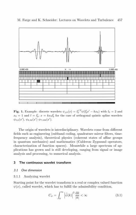
Wavelets have been developed in the beginning of eighties in France [31].This recent mathematical technique is based on group theory and squareintegrable representations, which allows the decomposition of a signal, or afield, into both space and scale, and possibly directions [14]. To motivatethe use of wavelets in relation with turbulence, we briefly recall some funda-mental ideas and mention several fields of applications. For details we referthe reader to textbooks [8,39,42]. From an abstract point of view waveletsconstitute new “atoms” and “molecules”, i.e. basic building blocks of vari-ous function spaces out of which some can be used to contruct orthogonalbases. The starting point is a function ψ(x), called mother wavelet. Thisfunction is assumed to be well-localized, i.e. ψ exhibits a fast decay for |x|tending to infinity, is oscillating, i.e. ψ has at least a vanishing integral(the mean value is zero) or better the first m moments of ψ vanish, and issmooth, i.e. ψ the Fourier transform of ψ exhibits fast decay in wavenumberspace |k|.

The mother wavelet then generates a family of wavelets ψl,x(x′) by di-latation (or contraction) by the parameter l > 0 and translation by theparameter x ∈ R, i.e. ψl,x(x′) = l−1/2ψ(x

′−xl ), where all wavelets be-

ing normalized in L2-norm. An example of such a family (for discrete land x) is depicted in Figure 1. The wavelet transform of a function f isthen defined as a convolution of the analysing wavelet with the signal f ,f(l, x) =

∫f(x′)ψl,x(x′)dx′. The wavelet coefficients f(l, x) measure the

fluctuations of f around the point x and scale (frequency) l. The functionf can be reconstructed as a linear combination of wavelets ψl,x(x′) with co-efficients f(l, x) [31], e.g. f(x) = 1/Cψ

∫ ∫f(l, x)ψl,x(x′)l−2dldx, Cψ being

a constant which depends on the wavelet ψ. Let us mention that due tothe localization of wavelets in physical space the behaviour of the signal atinfinity does not play any role. Therefore the wavelet analysis and synthe-sis can be performed locally as opposed to the Fourier transform where aglobal behaviour is intrinsically implicated through the nonlocal nature ofthe trigonometric functions.

“farge”2001/11/20page 457

�

�

�

�

�

�

�

�


Fig. 1. Example: discrete wavelets ψj,k(x) = lj/20 ψ(lj0x

′ − kx0) with l0 = 2 and

x0 = 1 and l = lj0, x = kx0lj0 for the case of orthogonal quintic spline wavelets

ψ5,6(x′), ψ6,32(x

′) ψ7,108(x′).

The origin of wavelets is interdisciplinary. Wavelets come from differentfields such as engineering (subband coding, quadrature mirror filters, time-frequency analysis), theoretical physics (coherent states of affine groupsin quantum mechanics) and mathematics (Calderon–Zygmund operators,characterization of function spaces). Meanwhile a large spectrum of ap-plications has grown and is still developing, ranging from signal or imageanalysis and processing, to numerical analysis.

3 The continuous wavelet transform

3.1 One dimension

3.1.1 Analyzing wavelet

Starting point for the wavelet transform is a real or complex valued functionψ(x), called wavelet, which has to fulfill the admissibility condition,

Cψ =∫ ∞

0

∣∣∣ψ(k)∣∣∣2 dk

|k| <∞ (3.1)

“farge”2001/11/20page 458

�

�

�

�

�

�

�

�


where

ψ(k) =12π

∫ ∞

−∞ψ(x)e−i2πkxdx (3.2)

denotes the Fourier transform. If ψ is integrable this implies that ψ haszero mean, ∫ ∞

−∞ψ(x)dx = 0 or ψ(k = 0) = 0. (3.3)

In practice however one also requires that the wavelet ψ should be well-localized in both physical and Fourier spaces, which implies smoothness.We also require that higher order moments of ψ vanish, i.e.∫ ∞

−∞xmψ(x)dx = 0 for m = 0,M (3.4)

which means that monomials up to degree M are exactly reproduced. InFourier space this property is equivalent to

dm

dkmψ(k)|k=0 = 0 for m = 0,M (3.5)

so that the Fourier transform of ψ decays smoothly at k = 0.

3.1.2 Wavelet analysis

From this function ψ, the so-called mother wavelet, we generate a family ofcontinuously translated and dilated wavelets, normalized in L2–norm

ψl,x(x′) = l−1/2ψ

(x′ − x

l

)for l > 0 and x ∈ R (3.6)

where l denotes the scale dilation parameter, corresponding to the width ofthe wavelet and x the translation parameter, corresponding to the positionof the wavelet.

In Fourier space this reads

ψl,x(k) =√lψ(lk)e−i2πkx (3.7)

where the contraction with 1/l is reflected in a dilation with l and thetranslation with x implies a rotation in the complex plane.

The continuous wavelet transform of a signal f is then defined as aconvolution of f with the wavelet family ψl,x

f(l, x) =∫ ∞

−∞f(x′)ψl,x(x

′)dx′ (3.8)

“farge”2001/11/20page 459

�

�

�

�

�

�

�

�


where ψl,x denotes in the case of complex valued wavelets the complexconjugate.

Using Parseval’s identity we also get

f(l, x) =∫ ∞

−∞f(k)ψl,x(k)dk (3.9)

so that the wavelet transform may be interpretated as a frequency decom-position using band pass filters ψl,x centered at frequency k = k0

l , wherek0 denotes the center of the wavelet in Fourier space, and having variablewidth ∆k

k , so for increasing scales the bandwidth is getting wider.

3.1.3 Wavelet synthesis

The admissibility condition (3.1) of ψ implies the existence of a finite energyreproducing kernel, see e.g. [8], which is a necessary condition for being ableto reconstruct a function from its wavelet coefficients. The signal can thusbe reconstructed entirely from its wavelet coefficients,

f(x) =1Cψ

∫ ∞

0

∫ ∞

−∞f(l, x)ψl,x(x′)

dldxl2

(3.10)

which is the inverse wavelet transform.

3.1.4 Energy conservation

There also holds an energy conservation like for Fourier transforms, i.e. aPlancherel identity, which means that the total energy of a signal can beeither calculated in physical space or in wavelet coefficient space,∫ ∞

−∞|f(x)|2dx =

1Cψ

∫ ∞

0

∫ ∞

−∞|f(l, x)|2 dldx

l2· (3.11)

This formula is also the starting point for the definition of wavelet spectra.

3.2 Higher dimensions

The theory of the continuous wavelet transform can be generalized in severaldimensions [44] using rotation in addition to dilatation and translation. Fora two-dimensional function f ∈ L2(R2) (constructions for higher dimensionsare analogous) we get

f(l, �x, θ) =∫ ∫

R2f(�x′)ψl,�x,θ(�x

′)d2�x′ for l > 0, θ ∈ [0, 2π[, �x ∈ R2

(3.12)

“farge”2001/11/20page 460

�

�

�

�

�

�

�

�


where the family of functions ψl,�x,θ is obtained from a single one ψ bydilatation with l−1, by translation by �x and by rotation of angle θ,

ψl,�x,θ(�x′) =1lψ

(Rθ

(�x′ − �x

l

))(3.13)

where Rθ denotes a rotation matrix.Analoguously to the one-dimensional case this transformation is invert-

ible and isometric, provided that ψ fulfills the admissibility condition

Cψ =∫ ∫

R2

∣∣∣ψ(�k)∣∣∣2 d2�k

|�k|2 <∞. (3.14)

In the following we restrict ourselves to isotropic real-valued wavelets, sothere is no more a dependence on θ. The wavelet coefficients can then becalculated using the formula

f(l, �x) =∫ ∫

R2f(�k)lψ(l�k)ei2π�k·�xd2�k (3.15)

where the Fourier transform of the wavelet ψl is essentially supported onan annulus a radius l−1.

The energy conservation reads∫ ∫R2

|f(�x)|2d�x =1Cψ

∫ ∞

0

∫ ∫R2

|f(l, �x)|2 dld2�x

l3(3.16)

and the function f can be recontructed entirely from its wavelet coefficientsby the relation

f(�x′) =1Cψ

∫ ∞

0

∫ ∫R2f(l, �x)ψl(�x′ − �x)

d2�xdll3

· (3.17)

3.3 Algorithm

To illustrate the practical implementation of the continuous wavelet trans-form we consider a one-dimensional signal f(x) sampled on a regular gridwith N = 2J points, i.e. f(i/2J) for i = 0, ..., 2J − 1 are given. We assumethe signal to be periodic and compute the wavelet coefficients by meansof the Fast Fourier Transform (FFT). The large scale corresponds to thedomaine size which is by construction equal to 1. The smaller scales arediscretized logarithmically,

lj = l−j0 j ≥ 0. (3.18)

The choise of l0 is determined by the reconstruction formula to ensure agiven precision for the reconstruction of the signal by a discretized version

“farge”2001/11/20page 461

�

�

�

�

�

�

�

�


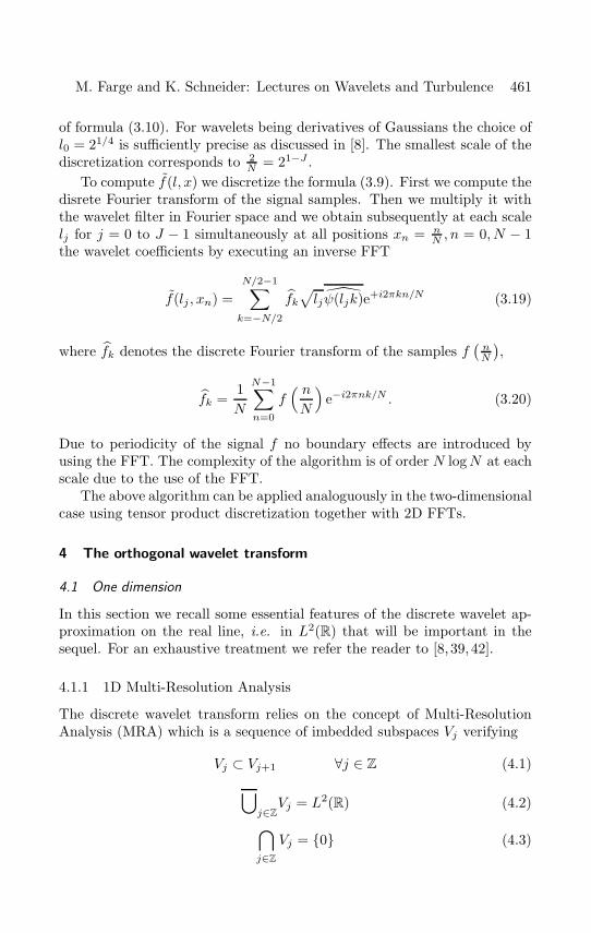
of formula (3.10). For wavelets being derivatives of Gaussians the choice ofl0 = 21/4 is sufficiently precise as discussed in [8]. The smallest scale of thediscretization corresponds to 2

N = 21−J .To compute f(l, x) we discretize the formula (3.9). First we compute the

disrete Fourier transform of the signal samples. Then we multiply it withthe wavelet filter in Fourier space and we obtain subsequently at each scalelj for j = 0 to J − 1 simultaneously at all positions xn = n

N , n = 0, N − 1the wavelet coefficients by executing an inverse FFT

f(lj , xn) =N/2−1∑k=−N/2

fk√ljψ(ljk)e+i2πkn/N (3.19)

where fk denotes the discrete Fourier transform of the samples f(nN

),

fk =1N

N−1∑n=0

f( nN

)e−i2πnk/N . (3.20)

Due to periodicity of the signal f no boundary effects are introduced byusing the FFT. The complexity of the algorithm is of order N logN at eachscale due to the use of the FFT.

The above algorithm can be applied analoguously in the two-dimensionalcase using tensor product discretization together with 2D FFTs.

4 The orthogonal wavelet transform

4.1 One dimension

In this section we recall some essential features of the discrete wavelet ap-proximation on the real line, i.e. in L2(R) that will be important in thesequel. For an exhaustive treatment we refer the reader to [8, 39, 42].

4.1.1 1D Multi-Resolution Analysis

The discrete wavelet transform relies on the concept of Multi-ResolutionAnalysis (MRA) which is a sequence of imbedded subspaces Vj verifying

Vj ⊂ Vj+1 ∀j ∈ Z (4.1)

⋃j∈Z

Vj = L2(R) (4.2)

⋂j∈Z

Vj = {0} (4.3)

“farge”2001/11/20page 462

�

�

�

�

�

�

�

�


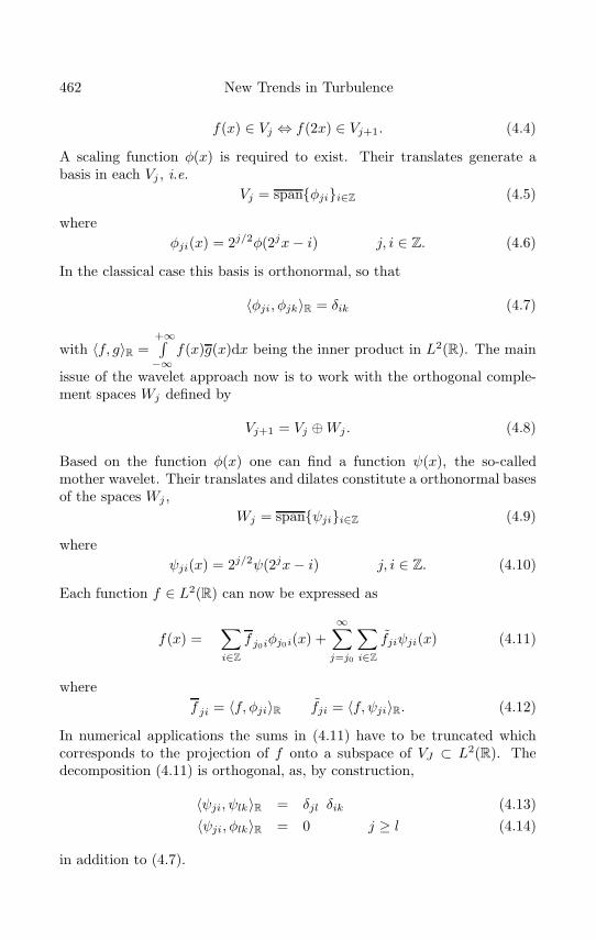
f(x) ∈ Vj ⇔ f(2x) ∈ Vj+1. (4.4)

A scaling function φ(x) is required to exist. Their translates generate abasis in each Vj , i.e.

Vj = span{φji}i∈Z (4.5)

whereφji(x) = 2j/2φ(2jx− i) j, i ∈ Z. (4.6)

In the classical case this basis is orthonormal, so that

〈φji, φjk〉R = δik (4.7)

with 〈f, g〉R =+∞∫−∞

f(x)g(x)dx being the inner product in L2(R). The main

issue of the wavelet approach now is to work with the orthogonal comple-ment spaces Wj defined by

Vj+1 = Vj ⊕Wj . (4.8)

Based on the function φ(x) one can find a function ψ(x), the so-calledmother wavelet. Their translates and dilates constitute a orthonormal basesof the spaces Wj ,

Wj = span{ψji}i∈Z (4.9)

whereψji(x) = 2j/2ψ(2jx− i) j, i ∈ Z. (4.10)

Each function f ∈ L2(R) can now be expressed as

f(x) =∑i∈Z

f j0iφj0i(x) +∞∑j=j0

∑i∈Z

fjiψji(x) (4.11)

wheref ji = 〈f, φji〉R fji = 〈f, ψji〉R. (4.12)

In numerical applications the sums in (4.11) have to be truncated whichcorresponds to the projection of f onto a subspace of VJ ⊂ L2(R). Thedecomposition (4.11) is orthogonal, as, by construction,

〈ψji, ψlk〉R = δjl δik (4.13)〈ψji, φlk〉R = 0 j ≥ l (4.14)

in addition to (4.7).

“farge”2001/11/20page 463

�

�

�

�

�

�

�

�


4.1.2 Regularity and local decay of wavelet coefficients

The relation between the local or global regularity of a function and thedecay of its wavelet coefficients is well known. The global regularity di-rectly determines the error being made when the wavelet sum is truncatedat some scale. Depending on the type of norm and whether global or lo-cal characterization is concerned, various relations of this kind have beendeveloped, see e.g. [8, 39, 42] for an overview. As an example we considerthe case of an α-Lipschitz function, with α ≥ 1 [33]. Suppose f ∈ L2(R),then for [a, b] ⊂ R the function f is α-Lipschitz for any x0 ∈ [a, b], i.e.|f(x0 + h) − f(x0)| ≤ C|h|α, if and only if there exists a constant A suchthat |〈f, ψji〉| ≤ A2−jα−

12 for any (j, i) with i

2j ∈]a, b[. This shows the rela-tion between the local regularity of a function and the decay of its waveletcoefficients in scale. The adaptive discretization discussed in the presentlecture notes is precisely based on taking into account spatially varyingregularity of the solution through a variable cut off in scale of its waveletseries.

4.2 Higher dimensions

This section consists of an extension of the previously presented one-dimen-sional construction to higher dimensions. For simplicity, we will consideronly the two-dimensional case, since higher dimensions can be treated anal-ogously [8, 39, 42]. We start with a brief description of the constructionprinciple and then turn in more detail to the two-dimensional case withperiodicity, which is relevant for the subsequent applications.

4.2.1 Tensor product construction

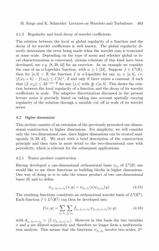
Having developed a one-dimensional orthonormal basis ψji of L2(R) onewould like to use these functions as building blocks in higher dimensions.One way of doing so is to take the tensor product of two one-dimensionalbases [8] and to define

ψjx,jy,ix,iy(x, y) = ψjx,ix(x)ψjy ,iy(y). (4.15)

The resulting functions constitute an orthonormal wavelet basis of L2(R2).Each function f ∈ L2(R2) can then be developed into

f(x, y) =∑jx,ix

∑jy ,iy

fjx,jy,ix,iyψjx,jy ,ix,iy(x, y) (4.16)

with djx,jy,ix,iy = 〈f, ψjx,jy,ix,iy〉. However in this basis the two variablesx and y are dilated separately and therefore no longer form a multiresolu-tion analysis. This means that the functions ψjx,jy involve two scales, 2jx

“farge”2001/11/20page 464

�

�

�

�

�

�

�

�


and 2jy , and each of the functions is essentially supported on a rectanglewith these side lengths. Hence the decomposition is often called rectan-gular wavelet decomposition. This is closely related to the standard formof operators using the nomenclature of Beylkin [3]. From the algorithmicviewpoint this is equivalent to apply the one-dimensional wavelet transformto the rows and the columns of a matrix representing an operator or a two-dimensional function. For some applications such a basis is advantageous,for others not. For exemple in turbulence the notion of a scale has an im-portant meaning and one would like to have a unique scale assigned to eachbasis function.

4.2.2 2D Multi-Resolution Analysis

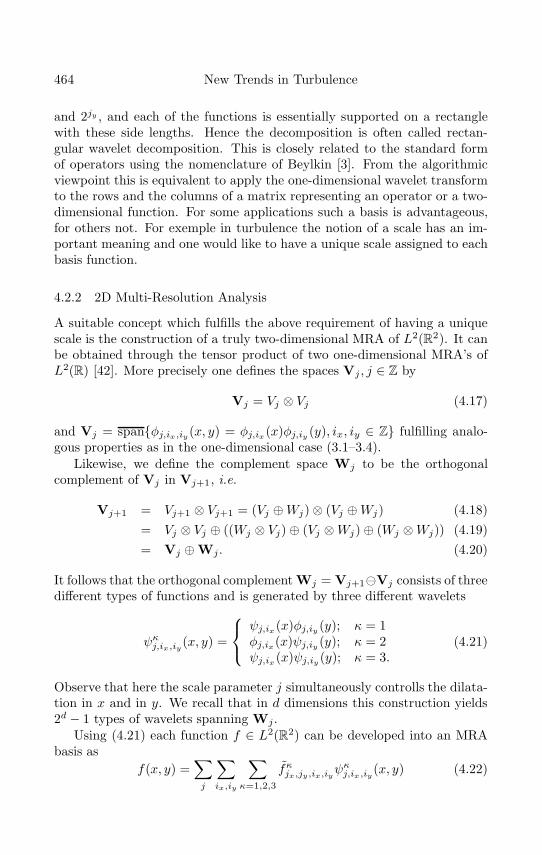
A suitable concept which fulfills the above requirement of having a uniquescale is the construction of a truly two-dimensional MRA of L2(R2). It canbe obtained through the tensor product of two one-dimensional MRA’s ofL2(R) [42]. More precisely one defines the spaces Vj , j ∈ Z by

Vj = Vj ⊗ Vj (4.17)

and Vj = span{φj,ix,iy(x, y) = φj,ix(x)φj,iy (y), ix, iy ∈ Z} fulfilling analo-gous properties as in the one-dimensional case (3.1–3.4).

Likewise, we define the complement space Wj to be the orthogonalcomplement of Vj in Vj+1, i.e.

Vj+1 = Vj+1 ⊗ Vj+1 = (Vj ⊕Wj) ⊗ (Vj ⊕Wj) (4.18)= Vj ⊗ Vj ⊕ ((Wj ⊗ Vj) ⊕ (Vj ⊗Wj) ⊕ (Wj ⊗Wj)) (4.19)= Vj ⊕ Wj. (4.20)

It follows that the orthogonal complement Wj = Vj+1 Vj consists of threedifferent types of functions and is generated by three different wavelets

ψκj,ix,iy(x, y) =

ψj,ix(x)φj,iy (y); κ = 1φj,ix(x)ψj,iy (y); κ = 2ψj,ix(x)ψj,iy (y); κ = 3.

(4.21)

Observe that here the scale parameter j simultaneously controlls the dilata-tion in x and in y. We recall that in d dimensions this construction yields2d − 1 types of wavelets spanning Wj.

Using (4.21) each function f ∈ L2(R2) can be developed into an MRAbasis as

f(x, y) =∑j

∑ix,iy

∑κ=1,2,3

fκjx,jy,ix,iyψκj,ix,iy(x, y) (4.22)

“farge”2001/11/20page 465

�

�

�

�

�

�

�

�


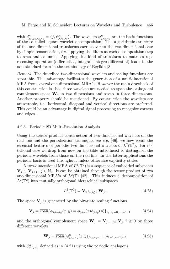
with dκjx,jy,ix,iy = 〈f, ψκj,ix,iy 〉. The wavelets ψκj,ix,iy are the basis functionsof the so-called square wavelet decomposition. The algorithmic structureof the one-dimensional transforms carries over to the two-dimensional caseby simple tensorisation, i.e. applying the filters at each decomposition stepto rows and columns. Applying this kind of transform to matrices rep-resenting operators (differential, integral, integro-differential) leads to thenon-standard form in the terminology of Beylkin [3].

Remark: The described two-dimensional wavelets and scaling functions areseparable. This advantage facilitates the generation of a multidimensionalMRA from several one-dimensional MRA’s. However the main drawback ofthis construction is that three wavelets are needed to span the orthogonalcomplement space Wj in two dimensions and seven in three dimensions.Another property should be mentioned. By construction the wavelets areanisotropic, i.e. horizontal, diagonal and vertical directions are preferred.This could be an advantage in digital signal processing to recognize cornersand edges.

4.2.3 Periodic 2D Multi-Resolution Analysis

Using the tensor product construction of two-dimensional wavelets on thereal line and the periodization technique, see e.g. [46], we now recall theessential features of periodic two-dimensional wavelets of L2(T2). For no-tational ease we drop from now on the tilde introduced to distinguish theperiodic wavelets from those on the real line. In the latter applications theperiodic basis is used throughout unless otherwise explicitly stated.

A two-dimensional MRA of L2(T2) is a sequence of embedded subspacesVj ⊂ Vj+1, j ∈ N0. It can be obtained through the tensor product of twoone-dimensional MRA’s of L2(T) [42]. This induces a decomposition ofL2(T2) into mutually orthogonal hierarchical subspaces

L2(T2) = V0 ⊕j≥0 Wj. (4.23)

The space Vj is generated by the bivariate scaling functions

Vj = span{φj,ix,iy(x, y) = φj,ix(x)φj,iy (y)}ix,iy=0,...,2j−1 (4.24)

and the orthogonal complement space Wj = Vj+1 Vj , j ≥ 0 by threedifferent wavelets

Wj = span{ψκj,ix,iy (x, y)}ix,iy=0,...,2j−1,κ=1,2,3 (4.25)

with ψκj,ix,iy defined as in (4.21) using the periodic analogons.

“farge”2001/11/20page 466

�

�

�

�

�

�

�

�


Correspondingly, any function f ∈ L2(T2) which is at least continuouscan be projected onto VJ by collocation

fJ(x, y) =2J−1∑ix=0

2J−1∑iy=0

f

(ix2J,iy2J

)SJ,ix,iy (x, y) (4.26)

using the two-dimensional cardinal Lagrange function

Sj,ix,iy(x, y) = Sj,ix(x)Sj,iy (y). (4.27)

It can then be expressed as

fJ(x, y) = f0,0,0φ0,0,0(x, y) +J−1∑j=0

2j−1∑ix=0

2j−1∑iy=0

3∑κ=1

fκj,ix,iyψκj,ix,iy(x, y) (4.28)

with coefficients

fκj,ix,iy = 〈f, ψκj,ix,iy〉, f0,0,0 =∫

T2f(x, y)dxdy (4.29)

using that φ0,0,0 = 1.Representing a function in terms of wavelet coefficients has the following

advantages. Smooth functions yield rapid decay of the coefficients in scale(depending on the number of vanishing moments of ψji). At locations whereu develops a singularity or an “almost singularity” only local coefficientshave to be retained (depending on the decay of ψji in space). Second, allemployed basis functions are mutually orthogonal, a property which is thekeystone of the algorithms.

4.3 Algorithm

In case of a regular sampling and periodic functions, computations canbe done in physical space by periodizing the required filters (defined below)using Mallat’s algorithm [39]. For long filters it is more economical, however,to use fast convolution in Fourier space employing FFT. Following [46] wedescribe such a transformation together with a computational trick for itsacceleration [26]. The algorithm is based on the application of three discretefilters. The scaling coefficients cJ,k are computed by application of theinterpolation filter

IJn = 〈SJ,n, φJ,0〉, IJ = 2−3J/2I

(k

2j

), I(k) = S(k)/φ(k) (4.30)

to the sampled values {f( i2J )}i.

“farge”2001/11/2

page 467�

�

�

�

�

�

�

�


The filters

Gjn = 〈φj,n, ψj−1,0〉, Hjn = 〈φj,n, φj−1,0〉 (4.31)

are classically used for computing the wavelet transform. They can beobtained in physical space for compactly supported bases and in Fourierspace through

H(k) = φ(2k)/φ(k), G(k) = ψ(2k)/φ(k). (4.32)

The algorithm then reads

Step 0. FFT of the values {fi}i=0,...,2J−1 at the points {xi = i2J }i=0,...,2J−1

to the Fourier coefficients {fk}k=0,...,2J−1.

Step 1. Interpolation using the Lagrange function SJ(x) of the space VJby computation in Fourier space: application of IJ gives (fJ )k, k =0, . . . , 2J − 1.

Step 2. Application of Filters G and H in Fourier space (* indicating dou-ble length sequences)

(f∗J−1

)k

= Hk

(fJ

)k

k = 0, . . . , 2J − 1 (4.33)

(f∗J−1

)k

= Gk

(fJ

)k

k = 0, . . . , 2J − 1. (4.34)

Step 3. Instead of setting

fJ−1,i = f∗J−1,2i fJ−1,i = f∗

J−1,2i i = 0, . . . , 2J−1 − 1 (4.35)

in physical space, downsampling can be done directly in Fourier spacethrough

(fJ−1

)k

=(f∗J−1

)k

+(f∗J−1

)k+2J−1

k = 0, . . . , 2J−1 (4.36)

(fJ−1

)k

=(f∗J−1

)k

+(f∗J−1

)k+2J−1

k = 0, . . . , 2J−1. (4.37)

Step 4. Inverse FFT of lenght 2J−1 to get {fJ−1,i}i=0,...,2J−1−1.

Iterate steps 2 to 4 replacing J by j = J−1, . . . , 0. Observe that in thelast step 2−1 is replaced by 0 and (f0)0 = f0,0.

“farge”2001/11/20page 468

�

�

�

�

�

�

�

�


The use of (4.36, 4.37) instead of (4.35) leads to a speed up by a factor 6 withrespect to extracting the coefficients in physical space. The inverse trans-form is obtained by executing the above steps in reversed order omittingthe conjugate complex in (4.33, 4.34) and replacing Step 3 with upsamplingin Fourier space.

Part II

Statistical Analysis5 Classical tools

5.1 Methodology

Turbulence research is based on either laboratory or numerical experiments.Typical quantities measured to characterize turbulent flows are scalar fields(temperature, concentration, pressure, etc.), vector fields (velocity, vorticity,etc.), tensor fields (stress, strain, etc.).

5.1.1 Laboratory experiments

Laboratory experiments are done (e.g. in wind tunnels or water tank) us-ing flow visualisations and time measurements performed in few points ofthe flow (e.g. hot-wire anemometry, laser velocimetry). Flow visualiza-tions give mostly qualitative information. Time measurements give quan-titative information by accumulating well-sampled and well-converged timestatistics, although only at very few spatial locations. By checking Taylor’shypothesis, namely that the time fluctuations are small compared to themean flow velocity, one assumes that the time statistics can be identifiedwith the space statistics. This allows to compare laboratory measurementswith the predictions of the statistical theory of turbulence, and also withthe statistics obtained from numerical experiments.

5.1.2 Numerical experiments

Numerical experiments are based on the accepted assumption that Navier–Stokes is the fundamental equation of fluid dynamics whatever the flowregime. The turbulent regime is reached when the nonlinear advective termdominates the linear dissipative term (limit ν → 0 or Re ∝ 1/ν → ∞). Inthis highly nonlinear regime, Navier–Stokes solutions can only be computedby numerical approximation. The computation predicts the time evolutionof one flow realization only. Statistical analyses are performed afterwardsin three different ways:

“farge”2001/11/20page 469

�

�

�

�

�

�

�

�


• by computing spatial statistics of instanteneous turbulent fields, whichis valid only if the computational domain is much larger than theintegral scale where turbulence is produced;

• by computing time statistics of long flow history, which is valid onlyif the time evolution is much larger than the eddy turn over timecharacteristic of turbulent flow instabilities;

• by running a large number of numerical simulations for the same pa-rameter and flow configuration, but with different initial conditions.The ensemble averages are computed afterwards. This procedure re-quires a number of independant realisations sufficient to ensure thestationarity of the probability distribution.

5.2 Averaging procedure

Turbulent flows are characterized by their unpredictability, namely eachflow realization is different, although the statistics are reproducible as longas the flow configuration and parameters are the same. This is the reasonwhy turbulence models predict only statistical quantities.

Another essential characteristic of turbulent flows is their intermittency,i.e. the fact that we observe in each flow realization well localized strongevents (bursts). This intermittent behaviour is not very pronounced inthe velocity field, but becomes dominant when one considers the velocitygradients or the vorticity fields. They are characterized by non-Gaussianprobability distribution functions, whose tails correspond to the intermit-tent bursts. We think that the flow intermittency comes from the nonlineardynamics of turbulent flows which, for incompressible fluids, tend to formwell localized coherent vortices (vortex spots in two dimensions and vortextubes in three dimensions) which move around in a chaotic way resultingfrom their mutual interactions.

A crucial difficulty in turbulence modelling is to define averages ableto take into account intermittency. Actually the L2-norm averages, i.e.(∫ |f(x)|2dx)1/2), classically used in turbulence (e.g. two-point correlations,

second order structure functions, spectra) are “blind” to intermittency, be-cause the well localized strong events responsible for intermittency are toorare to affect the L2-norm, their weight remaining negligible in the integral.

To define averages able to take into account intermittency there are twopossible strategies:

• either to consider Lp-norms, i.e. ((∫ |f(x)|pdx)1/p) with p large

enough to have the values of the PDF tails (Probability DistributionFunction) contributing significantly to the integral;

“farge”2001/11/20page 470

�

�

�

�

�

�

�

�


• or to extract the rare (intermittent) events, responsible for the heavytails of the PDF, from the dense (non-intermittent) events, whichcontribute only to the center of the PDF, and perform classical L2-norm averages for the dense events only.

The second approach corresponds to conditional averages and requires acriterium to separate the rare events from the dense events. As we haveassumed that the intermittency of turbulent flows is due to the presence ofcoherent vortices, responsible for the rare events, we first need to identifythem in order to then be able to extract them.

As we have shown [15,17] the coherent vortices can be characterized bythe fact that they correpond to the strongest wavelet coefficients of the vor-ticity field. Based on this property we have defined a procedure to extractthem [19,21], which consists in retaining only those vorticity wavelet coeffi-cients ω which are larger than a threshold value ωT = (2Z log10N)1/2, withZ the total enstrophy and N the resolution (i.e. the number of grid pointsor wavelet coefficients). We then verify that the PDF of the discarded co-efficients, i.e. those smaller than the treshold ωT which correspond to thedense non-intermittent events, is actually Gaussian.

5.3 Statistical diagnostics

5.3.1 Probability Distribution Function (PDF)

To motivate the introduction of a probability space (Ξ,F ,P) we consider:

• the set of all possible configurations of the flow, i.e. the phase spaceof the Navier–Stokes equations, denoted by Ξ;

• the collection F of all experiments with a definite outcome which havebeen performed, called the flow realisations;

• a probability measure P assigned to F , such that P(Ø) = 0 andP(Ξ) = 1, which assigns a probability to each experiment which hasbeen performed.

We consider a stationary, homogeneous and isotropic random fieldf(ξ, �x, t) ∈ F , with ξ ∈ Ξ, �x ∈ Rn and t ∈ R+

0 . For fixed ξ the func-tion f(�x, t) is called a realization of the random field or a sample, e.g. onecomponent of the velocity field.

Definition of the PDF: Using the probability measure P we define the dis-tribution function F (g) = P(−∞ < f ≤ g, f ∈ Ξ) which measures theprobability of f having a value less or equal to g.

“farge”2001/11/20page 471

�

�

�

�

�

�

�

�


5.3.2 Radon–Nikodyn’s theorem

If the probability measure P is absolutely continuous, there exists a proba-bility density p of P such that p(f) = dP

df , which corresponds to the deriva-tive dF

dg of the distribution F , i.e. p(f)df = P(f < g ≤ f + df, g ∈ Ξ).

The probability density is normalized such that∫

Rp(x)dx = 1.

5.3.3 Definition of the joint probability

Let f and g be two random fields, one can define the joint probability

F (f, g) = P(−∞ < f ′ ≤ f, −∞ < g′ ≤ g, [f ′, g′] ∈ Ξ).

The corresponding joint probability density function is given by p(f, g) =p(f)p(g) − p(f ∩ g) (Bayes’ theorem). If f and g are independent andidentically distributed (i.i.d.), then p(f, g) = p(f)p(g).

5.3.4 Statistical moments

The q-th order moments of the random field f are defined as

Mq(f) = 〈f q〉 =∫f qp(f)df. (5.1)

If f ∈ Ξ is ergodic the moments can also be expressed as space averages

Mq(f) =∫

(f(�x))qdn�x, (5.2)

where the integral is defined as

∫= lim

L→∞1L3

∫ L

0

∫ L

0

∫ L

0

, (5.3)

L being the size of the domain.Ratios of moments are defined, such as

Qp,q(f) =Mp(f)

(Mq(f))p/q· (5.4)

“farge”2001/11/20page 472

�

�

�

�

�

�

�

�


Classically one chooses q = 2, which leads to define statistical quantititiessuch as:

• skewness S = Q3,2(f);

• flatness F = Q4,2(f);

• hyperskewness Sh = Q5,2(f);

• hyperflatness Fh = Q6,2(f).

5.3.5 Structure functions

The p-th order structure function of a random scalar field f is defined as

Sp,f (�l) =∫

(f(�x +�l) − f(�x))pdn�x. (5.5)

5.3.6 Autocorrelation function

The autocorrelation function of the random scalar field f is defined as

R(�l) =∫f(�x)f(�x+�l)dn�x (5.6)

and for vector fields �f we get the two-point correlation tensor

Rij(�l) =∫fi(�x)fj(�x+�l)dn�x. (5.7)

Note that in turbulence the above quantity computed for the velocity field iscalled Reynolds stress tensor, and plays a key role in turbulence modelling.

5.3.7 Fourier spectrum

Definition of the spectrum: The spectrum of the random scalar field f isthe Fourier transform of its autocorrelation function:

Φ(�k) =1

(2π)n

∫R(�l)e−i�k·�ldn�l. (5.8)

For vector fields we obtain analogously

Φij(�k) =1

(2π)n

∫Rij(�l)e−i

�k·�ldn�l. (5.9)

One can integrate Φ(�k) on shells of radius k = |�k| which gives the one-dimensional spectrum

E(k) =∫

Φ(�k)kn−1dθ. (5.10)

“farge”2001/11/20page 473

�

�

�

�

�

�

�

�


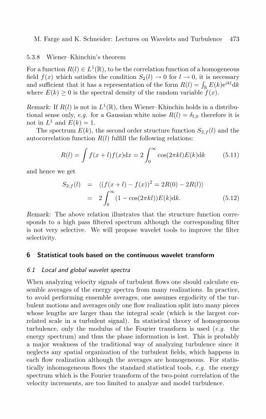
5.3.8 Wiener–Khinchin’s theorem

For a function R(l) ∈ L1(R), to be the correlation function of a homogeneousfield f(x) which satisfies the condition S2(l) → 0 for l → 0, it is necessaryand sufficient that it has a representation of the form R(l) =

∫RE(k)eikldk

where E(k) ≥ 0 is the spectral density of the random variable f(x).

Remark: If R(l) is not in L1(R), then Wiener–Khinchin holds in a distribu-tional sense only, e.g. for a Gaussian white noise R(l) = δl,0 therefore it isnot in L1 and E(k) = 1.

The spectrum E(k), the second order structure function S2,f (l) and theautocorrelation function R(l) fulfill the following relations:

R(l) =∫f(x+ l)f(x)dx = 2

∫ ∞

0

cos(2πkl)E(k)dk (5.11)

and hence we get

S2,f (l) = 〈(f(x+ l) − f(x))2 = 2R(0) − 2R(l)〉= 2

∫ ∞

0

(1 − cos(2πkl))E(k)dk. (5.12)

Remark: The above relation illustrates that the structure function corre-sponds to a high pass filtered spectrum although the corresponding filteris not very selective. We will propose wavelet tools to improve the filterselectivity.

6 Statistical tools based on the continuous wavelet transform

6.1 Local and global wavelet spectra

When analyzing velocity signals of turbulent flows one should calculate en-semble averages of the energy spectra from many realizations. In practice,to avoid performing ensemble averages, one assumes ergodicity of the tur-bulent motions and averages only one flow realization split into many pieceswhose lengths are larger than the integral scale (which is the largest cor-related scale in a turbulent signal). In statistical theory of homogeneousturbulence, only the modulus of the Fourier transform is used (e.g. theenergy spectrum) and thus the phase information is lost. This is probablya major weakness of the traditional way of analyzing turbulence since itneglects any spatial organization of the turbulent fields, which happens ineach flow realization although the averages are homogeneous. For statis-tically inhomogeneous flows the standard statistical tools, e.g. the energyspectrum which is the Fourier transform of the two-point correlation of thevelocity increments, are too limited to analyze and model turbulence.

“farge”2001/11/20page 474

�

�

�

�

�

�

�

�


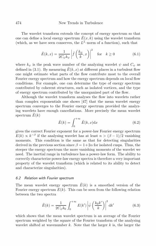
The wavelet transform extends the concept of energy spectrum so thatone can define a local energy spectrum E(x, k) using the wavelet transform(which, as we have seen conserves, the L2–norm of a function), such that

E(k, x) =1

2Cψkψ

∣∣∣∣f(kψk, x

)∣∣∣∣2 for k ≥ 0 (6.1)

where kψ is the peak wave number of the analyzing wavelet ψ and Cψ asdefined in (3.1). By measuring E(k, x) at different places in a turbulent flowone might estimate what parts of the flow contribute most to the overallFourier energy spectrum and how the energy spectrum depends on local flowconditions. For example, one can determine the type of energy spectrumcontributed by coherent structures, such as isolated vortices, and the typeof energy spectrum contributed by the unorganized part of the flow.

Although the wavelet transform analyses the flow into wavelets ratherthan complex exponentials one shows [47] that the mean wavelet energyspectrum converges to the Fourier energy spectrum provided the analyz-ing wavelets have enough cancellations. More precisely the mean waveletspectrum E(k)

E(k) =∫ +∞

0

E(k, x)dx (6.2)

gives the correct Fourier exponent for a power-law Fourier energy spectrumE(k) ∝ k−β if the analysing wavelet has at least n > (β − 1)/2 vanishingmoments. This condition is the same as that for detecting singularitiesderived in the previous section since β = 1+2α for isolated cusps. Thus, thesteeper the energy spectrum the more vanishing moments of the wavelet weneed. The inertial range in turbulence has a power-law form. The ability tocorrectly characterize power-law energy spectra is therefore a very importantproperty of the wavelet transform (which is related to its ability to detectand characterize singularities).

6.2 Relation with Fourier spectrum

The mean wavelet energy spectrum E(k) is a smoothed version of theFourier energy spectrum E(k). This can be seen from the following relationbetween the two spectra

E(k) =1

2Cψk0

∫ +∞

0

E(k′)∣∣∣∣ψ

(k0k

′

k

)∣∣∣∣2 dk′ (6.3)

which shows that the mean wavelet spectrum is an average of the Fourierspectrum weighted by the square of the Fourier transform of the analysingwavelet shifted at wavenumber k. Note that the larger k is, the larger the

“farge”2001/11/20page 475

�

�

�

�

�

�

�

�


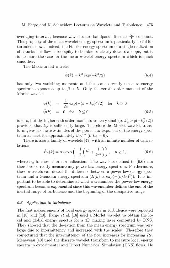
averaging interval, because wavelets are bandpass filters at ∆kk constant.

This property of the mean wavelet energy spectrum is particularly useful forturbulent flows. Indeed, the Fourier energy spectrum of a single realizationof a turbulent flow is too spiky to be able to clearly detects a slope, but itis no more the case for the mean wavelet energy spectrum which is muchsmoother.

The Mexican hat wavelet

ψ(k) = k2 exp(−k2/2) (6.4)

has only two vanishing moments and thus can correctly measure energyspectrum exponents up to β < 5. Only the zeroth order moment of theMorlet wavelet

ψ(k) =12π

exp(−(k − kψ)2/2) for k > 0

ψ(k) = 0 for k ≤ 0 (6.5)

is zero, but the higher n-th order moments are very small (∝ knψ exp(−k2ψ/2))

provided that kψ is sufficiently large. Therefore the Morlet wavelet trans-form gives accurate estimates of the power-law exponent of the energy spec-trum at least for approximately β < 7 (if kψ = 6).

There is also a family of wavelets [47] with an infinite number of cancel-lations

ψn(k) = αn exp(−1

2

(k2 +

1k2n

)), n ≥ 1, (6.6)

where αn is chosen for normalization. The wavelets defined in (6.6) cantherefore correctly measure any power-law energy spectrum. Furthermore,these wavelets can detect the difference between a power-law energy spec-trum and a Gaussian energy spectrum (E(k) ∝ exp(−(k/k0)2)). It is im-portant to be able to determine at what wavenumber the power-law energyspectrum becomes exponential since this wavenumber defines the end of theinertial range of turbulence and the beginning of the dissipative range.

6.3 Application to turbulence

The first measurements of local energy spectra in turbulence were reportedin [18] and [40]. Farge et al. [18] used a Morlet wavelet to obtain the lo-cal and global energy spectra for a 3D mixing layer computed by DNS.They showed that the deviation from the mean energy spectrum was verylarge due to intermittency and increased with the scales. Therefore theyconjectured that the intermittency of the flow increases for increasing Re.Meneveau [40] used the discrete wavelet transform to measure local energyspectra in experimental and Direct Numerical Simulation (DNS) flows. He

“farge”2001/11/20page 476

�

�

�

�

�

�

�

�


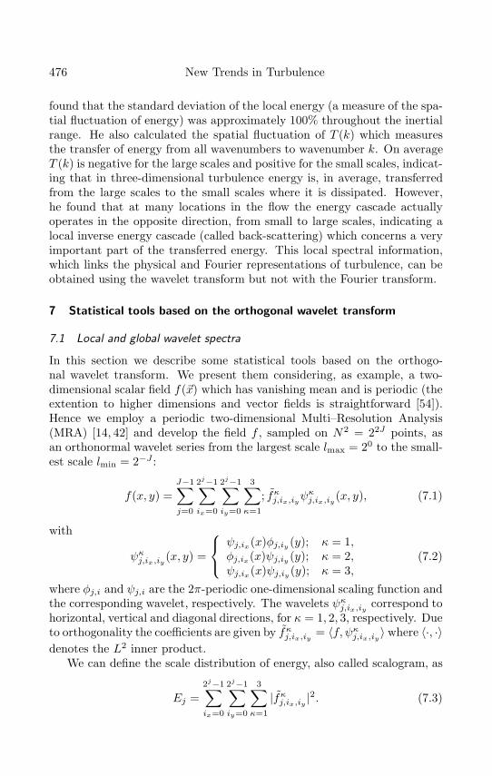
found that the standard deviation of the local energy (a measure of the spa-tial fluctuation of energy) was approximately 100% throughout the inertialrange. He also calculated the spatial fluctuation of T (k) which measuresthe transfer of energy from all wavenumbers to wavenumber k. On averageT (k) is negative for the large scales and positive for the small scales, indicat-ing that in three-dimensional turbulence energy is, in average, transferredfrom the large scales to the small scales where it is dissipated. However,he found that at many locations in the flow the energy cascade actuallyoperates in the opposite direction, from small to large scales, indicating alocal inverse energy cascade (called back-scattering) which concerns a veryimportant part of the transferred energy. This local spectral information,which links the physical and Fourier representations of turbulence, can beobtained using the wavelet transform but not with the Fourier transform.

7 Statistical tools based on the orthogonal wavelet transform

7.1 Local and global wavelet spectra

In this section we describe some statistical tools based on the orthogo-nal wavelet transform. We present them considering, as example, a two-dimensional scalar field f(�x) which has vanishing mean and is periodic (theextention to higher dimensions and vector fields is straightforward [54]).Hence we employ a periodic two-dimensional Multi–Resolution Analysis(MRA) [14, 42] and develop the field f , sampled on N2 = 22J points, asan orthonormal wavelet series from the largest scale lmax = 20 to the small-est scale lmin = 2−J :

f(x, y) =J−1∑j=0

2j−1∑ix=0

2j−1∑iy=0

3∑κ=1

; fκj,ix,iyψκj,ix,iy(x, y), (7.1)

with

ψκj,ix,iy(x, y) =

ψj,ix(x)φj,iy (y); κ = 1,φj,ix(x)ψj,iy (y); κ = 2,ψj,ix(x)ψj,iy (y); κ = 3,

(7.2)

where φj,i and ψj,i are the 2π-periodic one-dimensional scaling function andthe corresponding wavelet, respectively. The wavelets ψκj,ix,iy correspond tohorizontal, vertical and diagonal directions, for κ = 1, 2, 3, respectively. Dueto orthogonality the coefficients are given by fκj,ix,iy = 〈f, ψκj,ix,iy〉 where 〈·, ·〉denotes the L2 inner product.

We can define the scale distribution of energy, also called scalogram, as

Ej =2j−1∑ix=0

2j−1∑iy=0

3∑κ=1

|fκj,ix,iy |2. (7.3)

“farge”2001/11/20page 477

�

�

�

�

�

�

�

�


Introducing the discrete mean square wavelet coefficient at scale 2−j and atposition xix,iy = 2−j(ix + 1/2, iy + 1/2) as

f(2−j, 2−j(ix, iy)) =12((f1

j,ix,iy)2 + (f1j,ix+1,iy)2) +

12((f2

j,ix,iy)2

+(f2j,ix,iy+1)

2) + (f3j,ix,iy)2 (7.4)

we define a discrete local wavelet spectrum [10] by

E(kj , xix,iy) = f(2−j , 2−j(ix, iy))22j

∆kj· (7.5)

This quantitiy allows to study the space dependent spectral behaviour of f .By construction we have

E(kj) =2j−1∑ix=0

2j−1∑iy=0

E(kj , xix,iy). (7.6)

7.2 Relation with Fourier spectrum

Owing to the orthogonality of the wavelet decomposition, the total energyis preserved and we have E =

∑j Ej . To be able to relate the scale distri-

bution to the Fourier spectrum, we introduce the mean wavenumber k0 ofthe wavelet ψ, defined by

k0 =

∫ ∞0 k|ψ(k)|dk∫ ∞0

|ψ(k)|dk · (7.7)

Therewith each scale 2−j of the wavelet ψj is related to the mean wavenum-ber kj = k02j. With ∆kj =

√kjkj+1 − √

kjkj−1, describing the meanradial wavenumber of the three two-dimensional wavelets ψκj,ix,iy , we definethe global wavelet spectrum as

E(kj) = Ej/∆kj (7.8)

which is related with the Fourier energy spectrum by

E(k) =1k

∫ ∞

0

E(k′)|ψ(k0k′/k)|2dk′. (7.9)

The wavelet spectrum is a smoothed Fourier spectrum weighted with themodulus of the Fourier transform of the analyzing wavelet [47]. Note thatfor increasing wavenumbers the averaging interval becomes larger [14]. Asufficient condition, guaranteeing the global wavelet spectrum to be able to

“farge”2001/11/20page 478

�

�

�

�

�

�

�

�


detect the same power-law behaviour k−α as the Fourier spectrum, is thatψ has enough vanishing moments [47], i.e.∫ +∞

−∞xnψ(x)dx = 0 for 0 ≤ n ≤ α− 1

2· (7.10)

If this condition is not fulfilled the global wavelet spectrum saturates at thecritical cancellation order n and shows a power-law behaviour with a slopenot steeper than −2(n+ 1).

7.3 Intermittency measures

Useful diagnostics to quantify the intermittency of a field are the momentsof its wavelet coefficients at different scales j [53, 54],

Mp,j(f) =1

3 · 22j

2j−1∑ix=0

2j−1∑iy=0

3∑κ=1

|fκj,ix,iy |p. (7.11)

The sparsity of the wavelet coefficients at each scale can be measured andthe intermittency of the field f can be quantified using ratios of the momentsat different scales,

Qp,q,j(f) =Mp,j(f)

(Mq,j(f))p/q, (7.12)

which may be interpreted as quotient norms between different Lp- and Lq-spaces. Classically, one chooses q = 2 to define typical statistical quantitiesas a function of scale. Recall that for p = 4 we obtain the scale dependentflatness Fj = Q4,2,j which is equal to 3 for a Gaussian white noise at allscales j, which proves that this signal is not intermittent. The scale depen-dent skewness, hyperflatness and hyperskewness are obtained for p = 3, 5and 6, respectively. For intermittent signals Qp,q,j increases with j.

Part III

Computation8 Coherent vortex extraction

8.1 CVS filtering

In [21, 23] we have proposed a wavelet-based method, called CoherentVortex Simulation (CVS), to compute turbulent flows for regimes wherethe coherent vortices dominate the nonlinear dynamics. We first present

“farge”2001/11/20page 479

�

�

�

�

�

�

�

�


the CVS filtering, which extracts coherent vortices out of each flow real-ization. We then describe the CVS computation, which calculates the timeevolution of turbulent flows by deterministically computing the dynamics ofcoherent vortices, in an adaptive wavelet basis, and statistically modellingthe effect of the coherent velocity field onto the incoherent background flow.

8.1.1 Vorticity decomposition

We describe the wavelet algorithm to extract coherent vortices out of tur-bulent flows and consider as example the 3D case (for the 2D case referto [21]). We consider the vorticity field �ω(�x) = ∇ × �v, computed at res-olution N = 23J , N being the number of grid points and J the numberof octaves. Each component is developed into an orthogonal wavelet seriesfrom the largest scale lmax = 20 to the smallest scale lmin = 2J−1 using a3D multi-resolution analysis (MRA) [8, 14]:

ω(�x) = ω0,0,0φ0,0,0(�x)

+J−1∑j=0

2j−1∑ix=0

2j−1∑iy=0

2j−1∑iz=0

2n−1∑µ=1

ωµj,ix,iy ,izψµj,ix,iy,iz

(�x), (8.1)

with φj,ix,iyi,iz (�x) = φj,ix(x)φj,iy (y)φj,iz (z), and

ψµj,ix,iy,iz(�x) =

ψj,ix(x)φj,iy (y)φj,iz (z); µ = 1,φj,ix (x)ψj,iy (y)φj,iz (z); µ = 2,φj,ix (x)φj,iy (y)ψj,iz (z); µ = 3,ψj,ix(x)φj,iy (y)ψj,iz (z); µ = 4,ψj,ix(x)ψj,iy (y)φj,iz (z); µ = 5,φj,ix (x)ψj,iy (y)ψj,iz (z); µ = 6,ψj,ix(x)ψj,iy (y)ψj,iz (z); µ = 7,

(8.2)

where φj,i and ψj,i are the one-dimensional scaling function and the corre-sponding wavelet, respectively. Due to orthogonality, the scaling coefficientsare given by ω0,0,0 = 〈ω, φ0,0,0〉 and the wavelet coefficients are given byωµj,ix,iy,iz = 〈ω, ψµj,ix,iy,iz 〉, where 〈·, ·〉 denotes the L2-inner product.

8.1.2 Nonlinear thresholding

We then split the vorticity field into �ωC(�x) and �ωI(�x) by applying a nonlinearthresholding to the wavelet coefficients. The threshold is defined as ε =(4/3Z logN)1/2 and it only depends on the total enstrophy Z and on thenumber of grid points N without any adjustable parameters. The choice ofthis threshold is based on theorems [11,12] proving optimality of the waveletrepresentation to denoise signals in presence of Gaussian white noise, since

“farge”2001/11/20page 480

�

�

�

�

�

�

�

�


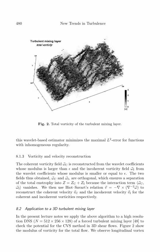
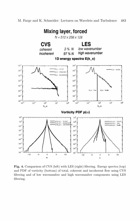
Fig. 2. Total vorticity of the turbulent mixing layer.

this wavelet-based estimator minimizes the maximal L2-error for functionswith inhomogeneous regularity.

8.1.3 Vorticity and velocity reconstruction

The coherent vorticity field �ωC is reconstructed from the wavelet coefficientswhose modulus is larger than ε and the incoherent vorticity field �ωI fromthe wavelet coefficients whose modulus is smaller or equal to ε. The twofields thus obtained, �ωC and �ωI, are orthogonal, which ensures a separationof the total enstrophy into Z = ZC + ZI because the interaction term 〈�ωC,�ωI〉 vanishes. We then use Biot–Savart’s relation �v = −∇ × (∇−2�ω) toreconstruct the coherent velocity �vC and the incoherent velocity �vI for thecoherent and incoherent vorticities respectively.

8.2 Application to a 3D turbulent mixing layer

In the present lecture notes we apply the above algorithm to a high resolu-tion DNS (N = 512 × 256 × 128) of a forced turbulent mixing layer [48] tocheck the potential for the CVS method in 3D shear flows. Figure 2 showthe modulus of vorticity for the total flow. We observe longitudinal vortex

“farge”2001/11/20page 481

�

�

�

�

�

�

�

�


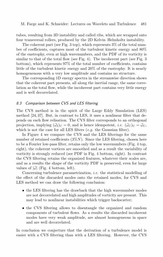
tubes, resulting from 3D instability and called ribs, which are wrapped ontofour transversal rollers, produced by the 2D Kelvin–Helmholtz instability.

The coherent part (see Fig. 3 top), which represents 3% of the total num-ber of coefficients, captures most of the turbulent kinetic energy and 80%of the enstrophy, even at high wavenumbers, and the PDF of its vorticity issimilar to that of the total flow (see Fig. 4). The incoherent part (see Fig. 3bottom), which represents 97% of the total number of coefficients, containslittle of the turbulent kinetic energy and 20% of the enstrophy. It is nearlyhomogenenous with a very low amplitude and contains no structure.

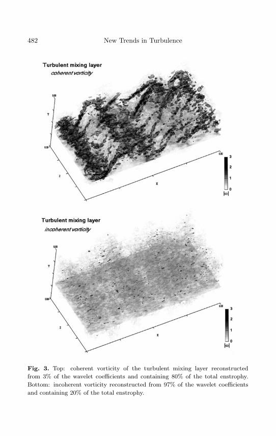
The corresponding 1D energy spectra in the streamwise direction showsthat the coherent part presents, all along the inertial range, the same corre-lation as the total flow, while the incoherent part contains very little energyand is well decorrelated.

8.3 Comparison between CVS and LES filtering

The CVS method is in the spirit of the Large Eddy Simulation (LES)method [24, 37]. But, in contrast to LES, it uses a nonlinear filter that de-pends on each flow relisation. The CVS filter corresponds to an orthogonalprojection, implying (�ωI)C = 0, and is hence idempotent, i.e. (�ωC)C = �ωC,which is not the case for all LES filters (e.g. the Gaussian filter).

In Figure 4 we compare the CVS and the LES filterings for the samenumber of retained coefficients (3%N). Since the LES filtering, chosen hereto be a Fourier low-pass filter, retains only the low wavenumbers (Fig. 4 top,right), the coherent vortices are smoothed and as a result the variability ofvorticity is strongly reduced (see PDF in Fig. 4 bottom, right). In contrastthe CVS filtering retains the organized features, whatever their scales are,and as a results the shape of the vorticity PDF is preserved, even for largevalues of |�ω| (Fig. 4 bottom, left).

Concerning turbulence parametrization, i.e. the statistical modelling ofthe effect of the discarded modes onto the retained modes, for CVS andLES method we can draw the following conclusion:

• the LES filtering has the drawback that the high wavenumber modesare not decorrelated and high amplitudes of vorticity are present. Thismay lead to nonlinear instabilities which trigger backscatter;

• the CVS filtering allows to disentangle the organized and randomcomponents of turbulent flows. As a results the discarded incoherentmodes have very weak amplitude, are almost homogeneous in spaceand are well decorrelated.

In conclusion we conjecture that the derivation of a turbulence model iseasier with a CVS filtering than with a LES filtering. However, the CVS

“farge”2001/11/20page 482

�

�

�

�

�

�

�

�


Fig. 3. Top: coherent vorticity of the turbulent mixing layer reconstructed

from 3% of the wavelet coefficients and containing 80% of the total enstrophy.

Bottom: incoherent vorticity reconstructed from 97% of the wavelet coefficients

and containing 20% of the total enstrophy.

“farge”2001/11/20page 483

�

�

�

�

�

�

�

�


Fig. 4. Comparison of CVS (left) with LES (right) filtering. Energy spectra (top)

and PDF of vorticity (bottom) of total, coherent and incoherent flow using CVS

filtering and of low wavenumber and high wavenumber components using LES

filtering.

“farge”2001/11/20page 484

�

�

�

�

�

�

�

�


filtering requires a dynamically adaptive mesh refinement for solving Navier–Stokes. In the next section we present such a method based on the waveletrepresentation that we have developed for the 2D Navier–Stokes equations.

9 Computation of turbulent flows

9.1 Navier–Stokes equations

9.1.1 Velocity–pressure formulation

The Navier–Stokes equation written in primitive variable formulation (ve-locity and pressure) describes the dynamics of a Newtonian (deformationproportional to velocity gradients) fluid

∂t�v + (�v · ∇)�v − ν∇2�v +1ρ∇p = �F (9.1)

and, if we suppose that the fluid is incompressible (constant density of thefluid elements), it is complemented by the continuity equation

∇ · �v = 0 (9.2)

where �v = (v1(�x, t), v2(�x, t), v3(�x, t)) and p(�x, t) denote the fluid velocityand the pressure respectively, at point �x = (x1, x2, x3) and time t. �F isthe field of external forces per unit mass, ρ the density and ν the constantkinematic viscosity. This system of coupled PDE’s must be supplementedby appropriate initial and boundary conditions.

9.1.2 Vorticity–velocity formulation

Taking the curl of (9.1), the pressure term can be eliminated and we get adynamical equation for the vorticity

∂t�ω + (�v · ∇)�ω − �ω · ∇�v − ν∇2�ω = ∇× �F . (9.3)

This is an advection-diffusion equation for the vorticity with an additionalterm �ω · ∇�v, which is responsible for the vortex stretching mechanism, i.e.vortex tubes can be stretched by velocity gradients, which leads to vorticityproduction. In two dimensions this term vanishes, because the vorticity isa pseudo-scalar �ω = (0, 0, ω3) perpendicular to the velocity gradients.

Taking the divergence of (9.1) and using the incompressibility of �v, weget a Poisson equation for the pressure which is used in many numericalschemes, such as projection methods or fractional step schemes [5, 56]

1ρ∇2p = −∇ · ((�v · ∇)�v). (9.4)

“farge”2001/11/20page 485

�

�

�

�

�

�

�

�


The relation �ω = ∇× �v can be inverted for a star shaped domain D usingPoincare’s lemma which leads to:

�v = −∇×∇−2�ω. (9.5)

The above relation can be expressed as a convolution product of the vorticitywith an operator K, called the Biot–Savart kernel, i.e. �v = K � �ω. As Kdecays slowly in physical space, i.e. as |�x|−2 in three dimensions and as|�x|−1 in two dimensions, the velocity is less localized than the vorticity.

9.2 Classical numerical methods

In the last 30 years the progress in numerical methods and the availability ofsupercomputers have had a significant impact on turbulence research. Forexample, the importance and role of coherent vortices in three-dimensionalturbulence has been established largely by high resolution numerical simula-tions [1,57,58]. Von Neumann’s vision, who had suggested in 1949 [45] thatturbulence could be simulated numerically, has become a reality. In contrastto the statistical theory of turbulence and to most laboratory experiments,which deal with L2-norm averaged quantities, numerical experiments dealwith non-averaged instantaneous quantities. Numerical experiments deter-ministically compute the evolution of one flow realization at a time, andperform the desired averages afterwards. There are two ways of comput-ing turbulent flows: either by Direct Numerical Simulation (DNS), or byModelled Numerical Simulation (MNS).

9.2.1 Direct Numerical Simulation (DNS)

In DNS one computes all degrees of freedom of the flow and both the nonlin-ear dynamics and the linear dissipation are fully resolved by computing thetime evolution of all these degrees of freedom. The DNS schemes currentlyin use may be classified into three categories:

• spectral and pseudo-spectral schemes;

• finite-difference, -volume, and -element methods;

• Lagrangian methods, e.g. vortex methods and contour dynamics.

The various methods are characterized by differences in their numericalcomplexity, accuracy and flexibility. Using DNS the evolution of all scalesof turbulent flows can only be calculated for moderate Reynolds numberswith present supercomputers. The severe limit of DNS is that the number ofdegrees of freedom N for a regular discretization depends on the Reynoldsnumber Re, such that N ∼ Re for two-dimensional flows and N ∼ Re9/4

“farge”2001/11/20page 486

�

�

�

�

�

�

�

�


for the three-dimensional case. At present only moderate Reynolds numberflows (Re ∼ 103 in three dimensions) can be simulated using DNS. Althoughmost flows of engineering interest have higher Reynolds numbers (Re ∼ 108),some physical insight can be gained from studying DNS of only moderateRe flows. However, laboratory experiments have shown that new behaviourappears in the range Re ∼ 104−105 [9]. As the number of degrees of freedomscales with Reynolds number, the simulation of such high Reynolds numberflows in two or three dimensions requires schemes employing some sort ofadaptive discretization.

To our knowledge no current non-wavelet DNS methods use a spatialdiscretization that adapts to the dynamics and structure of the flow. In [30]we have proposed an adaptive wavelet scheme for nonlinear PDE’s and wehave extended it to the two-dimensional Navier–Stokes equations [28, 51].Since the wavelet basis functions are localized in both physical and spectralspaces this approach is a compromise between grid-point methods and spec-tral methods. The adaptive wavelet method is well suited for turbulencesimulations because the characteristic structures encountered in turbulentflows are localized coherent vortices evolving under a multiscale nonlineardynamics. Thus the space- and scale-adaptivity of the wavelet basis shouldbe very efficient at representing turbulence structures and their dynamics.The fact that the basis is adapted to the solution and follows the time evo-lution of coherent vortices corresponds to a combination of both Eulerianand Lagrangian approaches.

9.2.2 Modelled Numerical Simulation (MNS)

In MNS, e.g. Unsteady Reynolds Averaged Navier–Stokes (URANS), LESand nonlinear Galerkin methods, one supposes that many modes can bediscarded, provided that some term(s) or some new equation(s) are addedto model the effect of the discarded modes onto the retained modes.

The time evolution of the resolved modes is deterministically computedusing the same numerical methods as for DNS. Concerning the discardedmodes, one supposes that they are slaved to the retained modes and pas-sively follow their motion. Consequently the dynamics of the unresolvedmodes cannot become unstable and grow in such a way that they woulddeterministically affect the evolution of the resolved modes. To ensure thisone should check that the unresolved modes have reached a statistical equi-librium state and are sufficiently decorrelated. In this case it is no longernecessary to compute the evolution of the unresolved modes in detail be-cause, if they are in statistical equilibrium, their effect onto the retainedmodes can be entirely characterized by their averages. The model describingthe effect of the unresolved modes onto the resolved modes can be specifiedonce the averaged quantities of the unresolved modes can be parametrized

“farge”2001/11/20page 487

�

�

�

�

�

�

�

�


as a function of the resolved modes.

“farge”2001/11/20page 488

�

�

�

�

�

�

�

�


Remark: Ideally, in order to reduce the computational cost as much aspossible, the number of resolved modes should be much smaller than thenumber of discarded modes and should increase more slowly with Re thanthe total number of modes does.

9.3 Coherent Vortex Simulation (CVS)

9.3.1 Principle of CVS

Coherent Vortex Simulation (CVS) deterministically computes the evolutionof the coherent vorticity �ωC and statistically models the effect of the incoher-ent vorticity �ωI and velocity �vI. In the following we apply the CVS methodto compute 2D turbulent flows. We filter the two-dimensional Navier–Stokesequations using CVS filtering and obtain the evolution equation for the co-herent vorticity ωC:

∂tωC + ∇ · (ω�v)C − ν∇2ωC = ∇× �FC (9.6)∇ · �vC = 0.

To model the effect of the discarded coefficients, which corresponds to theincoherent stress, we propose (as in LES) to use a Boussinesq ansatz. Forthe nonlinear term we use Leonard’s triple decomposition, because the non-linear term is computed with the same adapted grid as the linear term (i.e.without dealiasing). We decompose the nonlinear term of (9.6) into

(ω�v)C = ωC�vC + L+ C +R, (9.7)

where

L = (ωC�vC)C − ωC�vC,

C = (ωI�vC)C + (ωC�vI)C,

andR = (ωI�vI)C,

denoting the Leonard stress L, the cross stress C and the Reynolds stress R,respectively. The sum of these unknown terms corresponds to the incoherentstress:

τ = (ω�v)C − ωC�vC = L+ C +R, (9.8)

which describes the effect of the discarded incoherent terms on the re-solved coherent terms. Note that, due to the localization property of thewavelet representation, the Leonard stress L is actually negligible because(ωC�vC)C � ωC�vC [53].

“farge”2001/11/20page 489

�

�

�

�

�

�

�

�


The filtered Navier–Stokes equations (9.6) can be rewritten as:

∂tωC + ∇ · (ωC�vC) − ν∇2ωC = ∇× �FC −∇ · τ (9.9)∇ · �vC = 0.

9.3.2 CVS without turbulence model

If we consider a very small threshold, there is no longer any need to modelthe effect of the incoherent part because the incoherent stress is then negli-gible, and in this case CVS becomes DNS. Note that even when the waveletthreshold tends to zero, the number of discarded incoherent modes maystill be large, due to the excellent compression properties of the waveletrepresentation for turbulent flows. This is reflected by the fact that manywavelet coefficients are essentially zero and can therefore be discarded with-out loosing a significant amount of enstrophy.

To obtain the coherent variables ωC and �vC we deterministically inte-grate (9.6) since the variables are non-Gaussian and correspond to a dy-namical system out of statistical equilibrium. We solve these equations inan adaptive wavelet basis [30, 51, 53] (cf. the next section). The separationinto coherent and incoherent components is performed at each time step.The adaptive wavelet basis retains only those wavelet modes correspondingto the coherent vortices. It is remapped at each time step in order to followtheir motions, in both space and scale. In fact, this numerical scheme com-bines the advantages of both the Eulerian representation, since it projectsthe solution onto an orthonormal basis, and the Lagrangian representation,since it follows the coherent vortices by adapting the basis at each time step.

9.3.3 CVS with turbulence model

Up to now no modelling has been done, and equation (9.9) is not closedas long as τ depends on the incoherent unresolved terms. To close it wepropose two possibilities to model τ .

• A Boussinesq ansatz as for the LES method:

we assume that τ is proportional to the negative gradient of the co-herent vorticity, i.e. τ = −νT∇ωC with νT a turbulent viscositycoefficient. The turbulent viscosity νT can be estimated, either usingSmagorinsky’s model [24], or taking νT proportional to the enstro-phy fluxes in wavelet space, such that, where enstrophy flows fromlarge to small scales, νT is positive, and, where enstrophy flows fromsmall to large scales (i.e. backscatter), νT becomes negative. Thissecond method for estimating the turbulent viscosity is in the spiritof Germano’s dynamical procedure used for LES [24].

“farge”2001/11/20page 490

�

�

�

�

�

�

�

�


• A Gaussian stochastic forcing term:

we choose τ to be proportional to the incoherent enstrophy ZI com-puted at the previous time step. This modelling is made possible sincethe time evolution of the incoherent background, characterized by thetime scale tI = (ZI)−1/2, is much slower than the characteristic timescale tC = (ZC)−1/2 of the coherent motions, because ZC � ZI. Thisbehaviour of the incoherent background had already been noticed, anddiscussed in comparison to Fourier filtering in [16, 53].

The CVS method relies on the assumption that the incoherent velocity re-mains Gaussian, which is true as long as the nonlinear interactions betweenthe incoherent modes remains weak. This assumption is valid in regionswhere the density of coherent vortices is sufficient, because the strain theyexert on the incoherent background flow then inhibits the development ofany nonlinearity there [34]. However, there may be regions, although small,where the density of coherent vortices is not sufficient to control the inco-herent nonlinear term. In this case, there are two solutions:

• to locally refine the wavelet basis in these regions in order to deter-ministically compute the effect of incoherent nonlinear term (no longerneglected), which will lead to the formation of new coherent vorticesby instability of the incoherent background flow;

• to directly model the formation of new coherent vortices by addinglocally to the wavelet coefficients the amount of coherent enstrophywhich has been transferred from the incoherent enstrophy by the non-linear instability. This procedure is similar to the wavelet forcing wehave proposed in [50].

10 Adaptive wavelet computation

10.1 Adaptive wavelet scheme for nonlinear PDE’s

This section presents in a general form the adaptive discretization proce-dure for nonlinear parabolic PDE’s. We consider initial value problems andrestrict ourself to periodic boundary conditions. The time discretization isdone using a classical finite difference scheme of semi-implicit type. Oneobtains a set of ODE’s or PDE’s in space which are then solved at eachtime step with a method of weighted residuals. The particular choice of thetrial and test functions defines the different kinds of integration methods.

We consider nonlinear parabolic evolution equation

∂tu+Ku− F (u) = 0 (10.1)

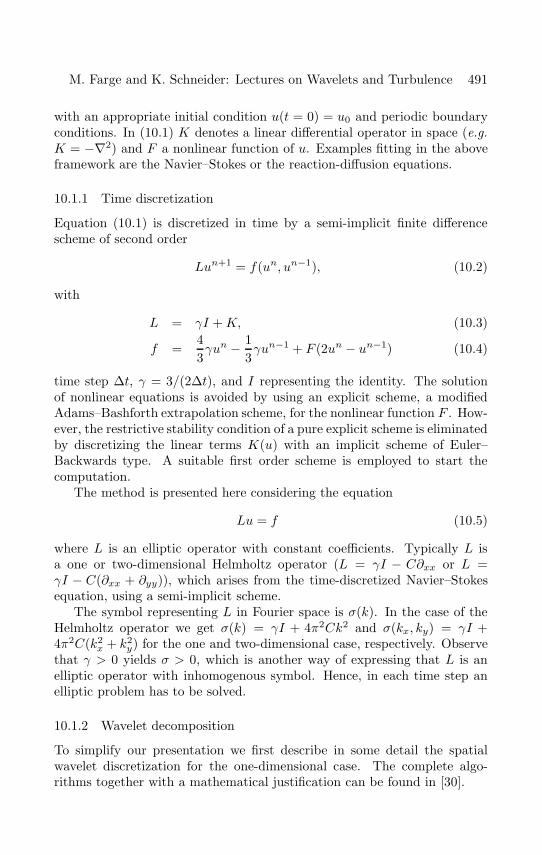
“farge”2001/11/20page 491

�

�

�

�

�

�

�

�


with an appropriate initial condition u(t = 0) = u0 and periodic boundaryconditions. In (10.1) K denotes a linear differential operator in space (e.g.K = −∇2) and F a nonlinear function of u. Examples fitting in the aboveframework are the Navier–Stokes or the reaction-diffusion equations.

10.1.1 Time discretization

Equation (10.1) is discretized in time by a semi-implicit finite differencescheme of second order

Lun+1 = f(un, un−1), (10.2)

with

L = γI +K, (10.3)

f =43γun − 1

3γun−1 + F (2un − un−1) (10.4)

time step ∆t, γ = 3/(2∆t), and I representing the identity. The solutionof nonlinear equations is avoided by using an explicit scheme, a modifiedAdams–Bashforth extrapolation scheme, for the nonlinear function F . How-ever, the restrictive stability condition of a pure explicit scheme is eliminatedby discretizing the linear terms K(u) with an implicit scheme of Euler–Backwards type. A suitable first order scheme is employed to start thecomputation.

The method is presented here considering the equation

Lu = f (10.5)

where L is an elliptic operator with constant coefficients. Typically L isa one or two-dimensional Helmholtz operator (L = γI − C∂xx or L =γI − C(∂xx + ∂yy)), which arises from the time-discretized Navier–Stokesequation, using a semi-implicit scheme.

The symbol representing L in Fourier space is σ(k). In the case of theHelmholtz operator we get σ(k) = γI + 4π2Ck2 and σ(kx, ky) = γI +4π2C(k2

x + k2y) for the one and two-dimensional case, respectively. Observe

that γ > 0 yields σ > 0, which is another way of expressing that L is anelliptic operator with inhomogenous symbol. Hence, in each time step anelliptic problem has to be solved.

10.1.2 Wavelet decomposition

To simplify our presentation we first describe in some detail the spatialwavelet discretization for the one-dimensional case. The complete algo-rithms together with a mathematical justification can be found in [30].

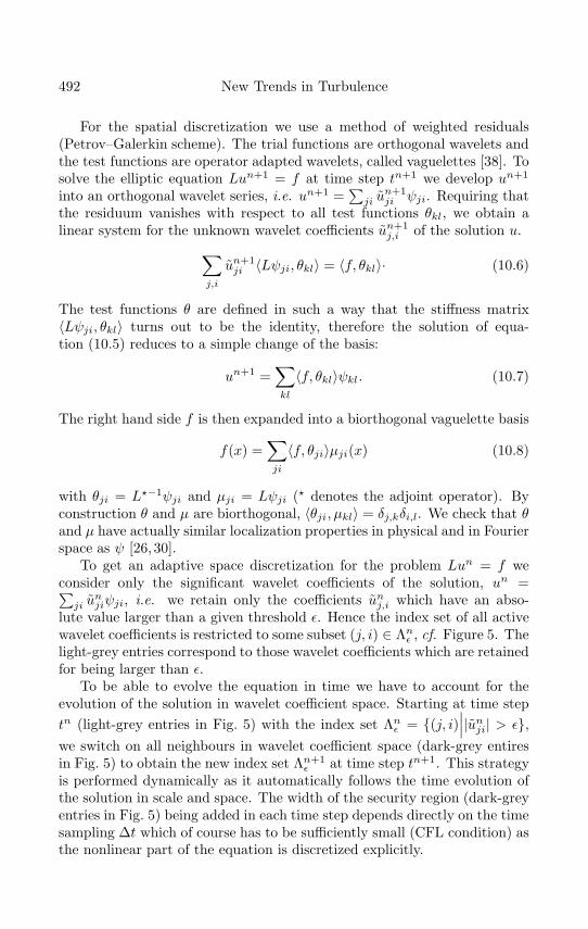
“farge”2001/11/20page 492

�

�

�

�

�

�

�

�


For the spatial discretization we use a method of weighted residuals(Petrov–Galerkin scheme). The trial functions are orthogonal wavelets andthe test functions are operator adapted wavelets, called vaguelettes [38]. Tosolve the elliptic equation Lun+1 = f at time step tn+1 we develop un+1

into an orthogonal wavelet series, i.e. un+1 =∑

ji un+1ji ψji. Requiring that

the residuum vanishes with respect to all test functions θkl, we obtain alinear system for the unknown wavelet coefficients un+1

j,i of the solution u.∑j,i

un+1ji 〈Lψji, θkl〉 = 〈f, θkl〉· (10.6)

The test functions θ are defined in such a way that the stiffness matrix〈Lψji, θkl〉 turns out to be the identity, therefore the solution of equa-tion (10.5) reduces to a simple change of the basis:

un+1 =∑kl

〈f, θkl〉ψkl. (10.7)

The right hand side f is then expanded into a biorthogonal vaguelette basis

f(x) =∑ji

〈f, θji〉µji(x) (10.8)

with θji = L�−1ψji and µji = Lψji (� denotes the adjoint operator). Byconstruction θ and µ are biorthogonal, 〈θji, µkl〉 = δj,kδi,l. We check that θand µ have actually similar localization properties in physical and in Fourierspace as ψ [26, 30].

To get an adaptive space discretization for the problem Lun = f weconsider only the significant wavelet coefficients of the solution, un =∑ji u

njiψji, i.e. we retain only the coefficients unj,i which have an abso-

lute value larger than a given threshold ε. Hence the index set of all activewavelet coefficients is restricted to some subset (j, i) ∈ Λnε , cf. Figure 5. Thelight-grey entries correspond to those wavelet coefficients which are retainedfor being larger than ε.

To be able to evolve the equation in time we have to account for theevolution of the solution in wavelet coefficient space. Starting at time steptn (light-grey entries in Fig. 5) with the index set Λnε = {(j, i)

∣∣∣|unji| > ε},we switch on all neighbours in wavelet coefficient space (dark-grey entiresin Fig. 5) to obtain the new index set Λn+1

ε at time step tn+1. This strategyis performed dynamically as it automatically follows the time evolution ofthe solution in scale and space. The width of the security region (dark-greyentries in Fig. 5) being added in each time step depends directly on the timesampling ∆t which of course has to be sufficiently small (CFL condition) asthe nonlinear part of the equation is discretized explicitly.

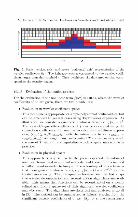
“farge”2001/11/20page 493

�

�

�

�

�

�

�

�


>-

>

-

j

i

Fig. 5. Scale (vertical axis) and space (horizontal axis) representation of the

wavelet coefficients uj,i. The light-grey entries correspond to the wavelet coeffi-

cients larger than the threshold ε. Their neighbors, the dark-grey entries, corre-

spond to the secutity region.

10.1.3 Evaluation of the nonlinear term

For the evaluation of the nonlinear term f(un) in (10.5), where the waveletcoefficients of un are given, there are two possibilities.

• Evaluation in wavelet coefficient space:

This technique is appropriate for simple polynomial nonlinearities, butcan be extended to general cases using Taylor series expansion. Asillustration we consider a quadratic nonlinear term, i.e. f(u) = u2.The wavelet/vaguelette coefficients of f can be calculated using theconnection coefficients, i.e. one has to calculate the bilinear expres-sion,

∑ji

∑kl ujiTjiklmnukl with the interaction tensor Tjiklmn =

〈ψjiψkl, θmn〉. Although many coefficients of T are zero or very small,the size of T leads to a computation which is quite untractable inpractice.

• Evaluation in physical space:

This approach is very similar to the pseudo-spectral evaluation ofnonlinear terms used in spectral methods, and therefore this methodis called pseudo-wavelet technique. The advantage of this scheme isthat more general nonlinear terms, e.g. f(u) = (1 − u)e−C/u, can betreated more easily. The prerequesites however are that fast adap-tive wavelet decomposition and reconstruction algorithms are avail-able. This means that functions can be reconstructed on a locallyrefined grid from a sparse set of their significant wavelet coefficientsand vice versa. The algorithms are described and analysed in detailin [30]. The method can be summarized as follows: starting from thesignificant wavelet coefficients of u, i.e. |uji| > ε, one reconstructs

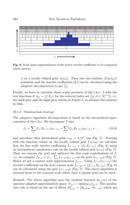
“farge”2001/11/20page 494

�

�

�

�

�

�

�

�


>-i

>

-

j

Fig. 6. Scale space representation of the active wavelet coeffcients to be computed

(dark entries).

u on a locally refined grid, u(xkl). Then one can evaluate f(u(xkl))pointwise and the wavelet coefficients of f can be calculated using theadaptive decomposition to get fji.

Finally, we have to calculate those scalar products of the r.h.s. f with thetest functions θ, uji = 〈f, θji〉 for the reduced index set {(j, i) ∈ Λn+1

ε }, i.e.the dark-grey and the light-grey entries in Figure 5, to advance the solutionin time.

10.1.4 Substraction strategy

The adaptive vaguelette decomposition is based on the hierarchical repre-sentation of the r.h.s. We decompose f into

fJ =∑i

〈fJ , θJ−1,i〉µJ−1,i +∑i

〈fJ , θJ−2,i〉µJ−2,i + ... (10.9)

and introduce then hierarchical grids xJk = k/2J (see Fig. 7). Startingwith the function values on the locally refined grid fJ(xJk) we calculatefirst the fine scale wavelet coefficients fJ−1,i = 〈fJ , θJ−1,i〉 (Fig. 6) usingan interpolatory quadrature rule on the locally refined grid {xJk} (Fig. 7).Then we coarsen the grid and subtract the fine scale contributions of f ,i.e. we compute fJ−1 = fJ −

∑i fJ−1,iµJ−1,i on the grid {xJ−1,k} (Fig. 7).

Hence we get a coarser scale approximation fJ−1. Using fJ−1(xJ−1,k) thewavelet coefficients on the next coarser scale fJ−2,i = 〈fJ−1, θJ−2,i〉 (Fig. 6)can be calculated using the grid {xJ−1,k} (Fig. 7). The above algorithm isiterated down to the coarsest scale where then a regular grid can be used.

Remark: The above algorithm uses the cardinal function SL;J(x) of theoperator adapted approximation space, VL;J = span{µji}j<J . The quadra-ture rule is based on the use of filters DJ

L;m = 〈SL;J,m, θJ−1,0〉 which are

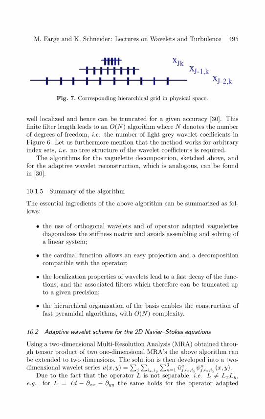
“farge”2001/11/20page 495

�

�

�

�

�

�

�

�


xJk xJ-1,kxJ-2,k

Fig. 7. Corresponding hierarchical grid in physical space.

well localized and hence can be truncated for a given accuracy [30]. Thisfinite filter length leads to an O(N) algorithm where N denotes the numberof degrees of freedom, i.e. the number of light-grey wavelet coefficients inFigure 6. Let us furthermore mention that the method works for arbitraryindex sets, i.e. no tree structure of the wavelet coefficients is required.

The algorithms for the vaguelette decomposition, sketched above, andfor the adaptive wavelet reconstruction, which is analogous, can be foundin [30].

10.1.5 Summary of the algorithm

The essential ingredients of the above algorithm can be summarized as fol-lows:

• the use of orthogonal wavelets and of operator adapted vaguelettesdiagonalizes the stiffness matrix and avoids assembling and solving ofa linear system;

• the cardinal function allows an easy projection and a decompositioncompatible with the operator;

• the localization properties of wavelets lead to a fast decay of the func-tions, and the associated filters which therefore can be truncated upto a given precision;

• the hierarchical organisation of the basis enables the construction offast pyramidal algorithms, with O(N) complexity.

10.2 Adaptive wavelet scheme for the 2D Navier–Stokes equations

Using a two-dimensional Multi-Resolution Analysis (MRA) obtained throu-gh tensor product of two one-dimensional MRA’s the above algorithm canbe extended to two dimensions. The solution is then developed into a two-dimensional wavelet series u(x, y) =

∑j

∑ix,iy

∑3κ=1 u

κj,ix,iy

ψκj,ix,iy (x, y).Due to the fact that the operator L is not separable, i.e. L �= LxLy,

e.g. for L = Id − ∂xx − ∂yy the same holds for the operator adapted

“farge”2001/11/20page 496

�

�

�

�

�

�

�

�


biorthogonal functions: θ(x, y) = L�−1ψ(x, y) �= θ(x)θ(y) and µ(x, y) =Lψ(x, y) �= µ(x)µ(y) and similarly for the filters SL and DL.

Now we extend the previouly described adaptive wavelet-vaguelette al-gorithm to solve the two-dimensional Navier–Stokes equations written invorticity-velocity formulation. Using this method the vorticity is decom-posed into a lacunary basis of orthogonal wavelets. Adaptivity means thatthe simulation uses only the minimum number of wavelet modes necessaryto represent the vorticity field at any given time and position (within a givenprecision ε). We will now use the reduced set of wavelet basis functions todirectly compute the evolution of the flow using the discretization proceduredescribed in the previous section.

We expand the vorticity ω into an orthogonal wavelet series (7.1) andapply a Petrov–Galerkin scheme with test functions

θκj,ix,iy (x, y) = (γ − ν∇2)−1ψκj,ix,iy(x, y) (10.10)

where γ = 3/(2∆t) The vaguelettes θ defined in (10.10) can be calculatedexplicitly in Fourier space and have localization properties similar to thoseof wavelets [27,42], i.e. in the case of spline wavelets they have exponentialdecay. The solution then reduces to the calculation of the coefficients

ωκ,n+1j,ix,iy

= 〈ωn+1, ψκj,ix,iy 〉 (10.11)

=⟨

43γωn − 1

3γωn−1, θκj,ix,iy

⟩− 〈�v∗ · ∇ω∗, θκj,ix,iy〉

with �v∗ = 2�vn − �vn−1 and ω∗ = 2ωn − ωn−1, using an adaptive two-dimensional vaguelette decomposition [4], i.e. only the coefficients ωκ,n+1

j,ix,iylarger than the threshold ε are calculated. The pyramidal decompositionalgorithm is based on a subtraction strategy applied to hierarchical nestedgrids using the cardinal Lagrange function of the operator-adapted multi-resolution analysis [27]. Subsequently, the vorticity field is reconstructed ona locally refined grid using the adaptive wavelet reconstruction.

The nonlinear term �v� ·∇ω� is computed by partial collocation [52]. Thispseudo-wavelet scheme can be sketched as follows: starting from the waveletcoefficients of ωn, ωn−1 we obtain the values of ω� on a locally refined gridthrough an inverse wavelet transform. Solving the Poisson equation using aPetrov–Galerkin scheme with test functions (∇2)−1ψκj,ix,iy(x, y), we get thewavelet coefficients of the stream function Ψ�. Note that these test functionsare rapidly decaying in physical space due to the vanishing moments ofthe wavelets. Applying an inverse adaptive wavelet transform, the streamfunction is reconstructed on a locally refined grid. Then the velocity �v�, thevorticity gradient ∇ω� and the nonlinear term �v� ·∇ω� are calculated usingfinite differences of 4th order on the adaptive grid. Finally, the right hand

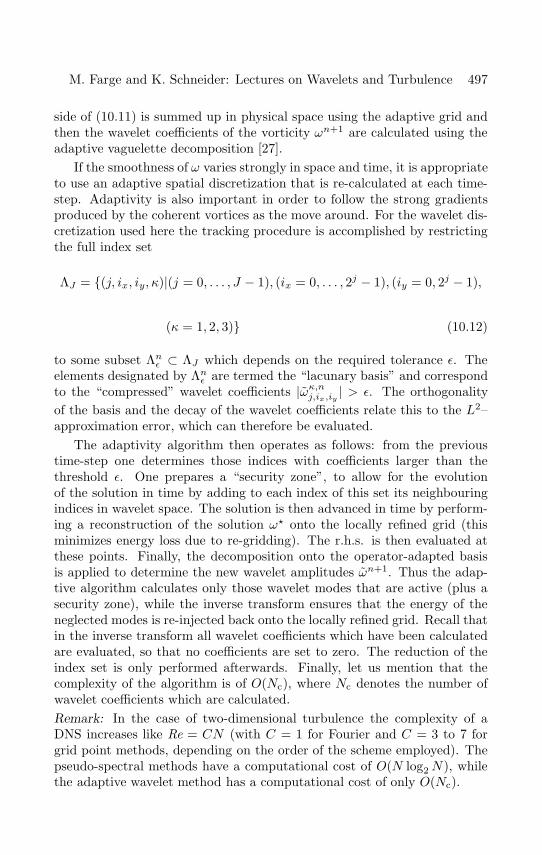
“farge”2001/11/20page 497

�

�

�

�

�

�

�

�


side of (10.11) is summed up in physical space using the adaptive grid andthen the wavelet coefficients of the vorticity ωn+1 are calculated using theadaptive vaguelette decomposition [27].

If the smoothness of ω varies strongly in space and time, it is appropriateto use an adaptive spatial discretization that is re-calculated at each time-step. Adaptivity is also important in order to follow the strong gradientsproduced by the coherent vortices as the move around. For the wavelet dis-cretization used here the tracking procedure is accomplished by restrictingthe full index set

ΛJ = {(j, ix, iy, κ)|(j = 0, . . . , J − 1), (ix = 0, . . . , 2j − 1), (iy = 0, 2j − 1),

(κ = 1, 2, 3)} (10.12)

to some subset Λnε ⊂ ΛJ which depends on the required tolerance ε. Theelements designated by Λnε are termed the “lacunary basis” and correspondto the “compressed” wavelet coefficients |ωκ,nj,ix,iy | > ε. The orthogonalityof the basis and the decay of the wavelet coefficients relate this to the L2–approximation error, which can therefore be evaluated.

The adaptivity algorithm then operates as follows: from the previoustime-step one determines those indices with coefficients larger than thethreshold ε. One prepares a “security zone”, to allow for the evolutionof the solution in time by adding to each index of this set its neighbouringindices in wavelet space. The solution is then advanced in time by perform-ing a reconstruction of the solution ω� onto the locally refined grid (thisminimizes energy loss due to re-gridding). The r.h.s. is then evaluated atthese points. Finally, the decomposition onto the operator-adapted basisis applied to determine the new wavelet amplitudes ωn+1. Thus the adap-tive algorithm calculates only those wavelet modes that are active (plus asecurity zone), while the inverse transform ensures that the energy of theneglected modes is re-injected back onto the locally refined grid. Recall thatin the inverse transform all wavelet coefficients which have been calculatedare evaluated, so that no coefficients are set to zero. The reduction of theindex set is only performed afterwards. Finally, let us mention that thecomplexity of the algorithm is of O(Nc), where Nc denotes the number ofwavelet coefficients which are calculated.Remark: In the case of two-dimensional turbulence the complexity of aDNS increases like Re = CN (with C = 1 for Fourier and C = 3 to 7 forgrid point methods, depending on the order of the scheme employed). Thepseudo-spectral methods have a computational cost of O(N log2N), whilethe adaptive wavelet method has a computational cost of only O(Nc).

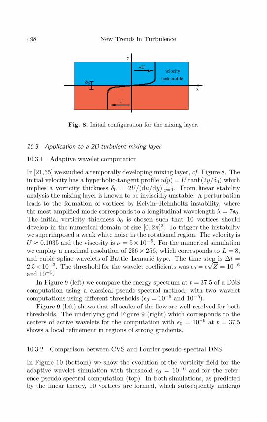
“farge”2001/11/20page 498

�

�

�

�

�

�

�

�


-U

δ0

velocity

tanh profile

+U

x

y

Fig. 8. Initial configuration for the mixing layer.

10.3 Application to a 2D turbulent mixing layer

10.3.1 Adaptive wavelet computation

In [21,55] we studied a temporally developing mixing layer, cf. Figure 8. Theinitial velocity has a hyperbolic-tangent profile u(y) = U tanh(2y/δ0) whichimplies a vorticity thickness δ0 = 2U/(du/dy)|y=0. From linear stabilityanalysis the mixing layer is known to be inviscidly unstable. A perturbationleads to the formation of vortices by Kelvin–Helmholtz instability, wherethe most amplified mode corresponds to a longitudinal wavelength λ = 7δ0.The initial vorticity thickness δ0 is chosen such that 10 vortices shoulddevelop in the numerical domain of size [0, 2π]2. To trigger the instabilitywe superimposed a weak white noise in the rotational region. The velocity isU ≈ 0.1035 and the viscosity is ν = 5× 10−5. For the numerical simulationwe employ a maximal resolution of 256× 256, which corresponds to L = 8,and cubic spline wavelets of Battle–Lemarie type. The time step is ∆t =2.5×10−3. The threshold for the wavelet coefficients was ε0 = ε

√Z = 10−6

and 10−5.In Figure 9 (left) we compare the energy spectrum at t = 37.5 of a DNS

computation using a classical pseudo-spectral method, with two waveletcomputations using different thresholds (ε0 = 10−6 and 10−5).

Figure 9 (left) shows that all scales of the flow are well-resolved for boththresholds. The underlying grid Figure 9 (right) which corresponds to thecenters of active wavelets for the computation with ε0 = 10−6 at t = 37.5shows a local refinement in regions of strong gradients.

10.3.2 Comparison between CVS and Fourier pseudo-spectral DNS

In Figure 10 (bottom) we show the evolution of the vorticity field for theadaptive wavelet simulation with threshold ε0 = 10−6 and for the refer-ence pseudo-spectral computation (top). In both simulations, as predictedby the linear theory, 10 vortices are formed, which subsequently undergo

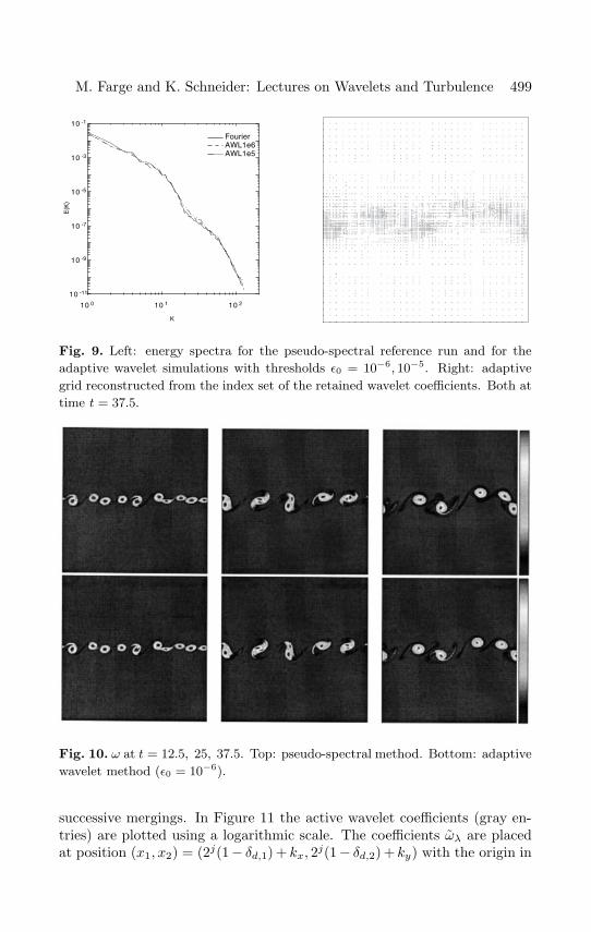
“farge”2001/11/20page 499

�

�

�

�

�

�

�

�


10 -11

10 -9

10 -7

10 -5

10 -3

10 -1

10 0 10 1 10 2

FourierAWL1e6AWL1e5

E(K

)

K

Fig. 9. Left: energy spectra for the pseudo-spectral reference run and for the

adaptive wavelet simulations with thresholds ε0 = 10−6, 10−5. Right: adaptive

grid reconstructed from the index set of the retained wavelet coefficients. Both at

time t = 37.5.

Fig. 10. ω at t = 12.5, 25, 37.5. Top: pseudo-spectral method. Bottom: adaptive

wavelet method (ε0 = 10−6).

successive mergings. In Figure 11 the active wavelet coefficients (gray en-tries) are plotted using a logarithmic scale. The coefficients ωλ are placedat position (x1, x2) = (2j(1− δd,1) + kx, 2j(1− δd,2) + ky) with the origin in

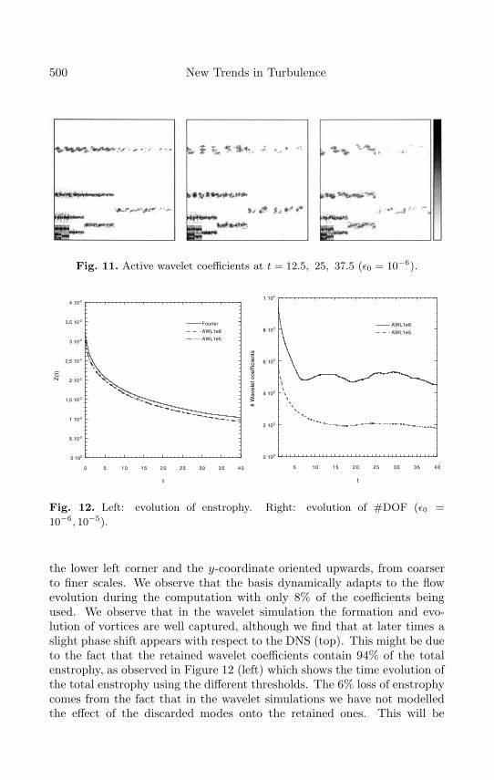
“farge”2001/11/20page 500

�

�

�

�

�

�

�

�


Fig. 11. Active wavelet coefficients at t = 12.5, 25, 37.5 (ε0 = 10−6).

0 100

5 10-3

1 10-2

1,5 10-2

2 10-2

2,5 10-2

3 10-2

3,5 10-2

4 10-2

0 5 10 15 20 25 30 35 40

Fourier

AWL1e6

AWL1e5

Z(t

)

t

0 100

2 103

4 103

6 103

8 103

1 104

5 10 15 20 25 30 35 40

AWL1e6

AWL1e5

# W

avel

et c

oeffi

cien

ts

t

Fig. 12. Left: evolution of enstrophy. Right: evolution of #DOF (ε0 =

10−6, 10−5).

the lower left corner and the y-coordinate oriented upwards, from coarserto finer scales. We observe that the basis dynamically adapts to the flowevolution during the computation with only 8% of the coefficients beingused. We observe that in the wavelet simulation the formation and evo-lution of vortices are well captured, although we find that at later times aslight phase shift appears with respect to the DNS (top). This might be dueto the fact that the retained wavelet coefficients contain 94% of the totalenstrophy, as observed in Figure 12 (left) which shows the time evolution ofthe total enstrophy using the different thresholds. The 6% loss of enstrophycomes from the fact that in the wavelet simulations we have not modelledthe effect of the discarded modes onto the retained ones. This will be

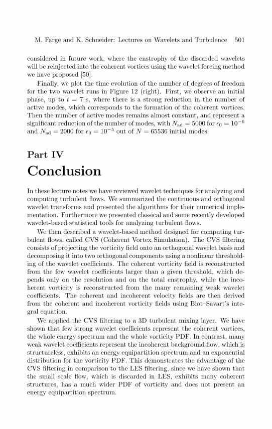
“farge”2001/11/20page 501

�

�

�

�

�

�

�

�


considered in future work, where the enstrophy of the discarded waveletswill be reinjected into the coherent vortices using the wavelet forcing methodwe have proposed [50].

Finally, we plot the time evolution of the number of degrees of freedomfor the two wavelet runs in Figure 12 (right). First, we observe an initialphase, up to t = 7 s, where there is a strong reduction in the number ofactive modes, which corresponds to the formation of the coherent vortices.Then the number of active modes remains almost constant, and represent asignificant reduction of the number of modes, withNad = 5000 for ε0 = 10−6

and Nad = 2000 for ε0 = 10−5 out of N = 65536 initial modes.

Part IV

Conclusion

In these lecture notes we have reviewed wavelet techniques for analyzing andcomputing turbulent flows. We summarized the continuous and orthogonalwavelet transforms and presented the algorithms for their numerical imple-mentation. Furthermore we presented classical and some recently developedwavelet-based statistical tools for analyzing turbulent flows.

We then described a wavelet-based method designed for computing tur-bulent flows, called CVS (Coherent Vortex Simulation). The CVS filteringconsists of projecting the vorticity field onto an orthogonal wavelet basis anddecomposing it into two orthogonal components using a nonlinear threshold-ing of the wavelet coefficients. The coherent vorticity field is reconstructedfrom the few wavelet coefficients larger than a given threshold, which de-pends only on the resolution and on the total enstrophy, while the inco-herent vorticity is reconstructed from the many remaining weak waveletcoefficients. The coherent and incoherent velocity fields are then derivedfrom the coherent and incoherent vorticity fields using Biot–Savart’s inte-gral equation.

We applied the CVS filtering to a 3D turbulent mixing layer. We haveshown that few strong wavelet coefficients represent the coherent vortices,the whole energy spectrum and the whole vorticity PDF. In contrast, manyweak wavelet coefficients represent the incoherent background flow, which isstructureless, exhibits an energy equipartition spectrum and an exponentialdistribution for the vorticity PDF. This demonstrates the advantage of theCVS filtering in comparison to the LES filtering, since we have shown thatthe small scale flow, which is discarded in LES, exhibits many coherentstructures, has a much wider PDF of vorticity and does not present anenergy equipartition spectrum.

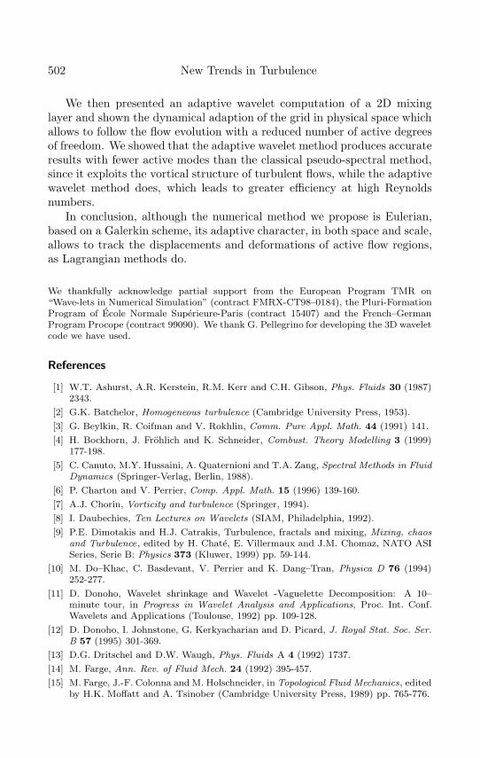
“farge”2001/11/20page 502

�

�

�

�

�

�

�

�


We then presented an adaptive wavelet computation of a 2D mixinglayer and shown the dynamical adaption of the grid in physical space whichallows to follow the flow evolution with a reduced number of active degreesof freedom. We showed that the adaptive wavelet method produces accurateresults with fewer active modes than the classical pseudo-spectral method,since it exploits the vortical structure of turbulent flows, while the adaptivewavelet method does, which leads to greater efficiency at high Reynoldsnumbers.

In conclusion, although the numerical method we propose is Eulerian,based on a Galerkin scheme, its adaptive character, in both space and scale,allows to track the displacements and deformations of active flow regions,as Lagrangian methods do.

We thankfully acknowledge partial support from the European Program TMR on“Wave-lets in Numerical Simulation” (contract FMRX-CT98–0184), the Pluri-FormationProgram of Ecole Normale Superieure-Paris (contract 15407) and the French–GermanProgram Procope (contract 99090). We thank G. Pellegrino for developing the 3D waveletcode we have used.

References

[1] W.T. Ashurst, A.R. Kerstein, R.M. Kerr and C.H. Gibson, Phys. Fluids 30 (1987)2343.

[2] G.K. Batchelor, Homogeneous turbulence (Cambridge University Press, 1953).

[3] G. Beylkin, R. Coifman and V. Rokhlin, Comm. Pure Appl. Math. 44 (1991) 141.

[4] H. Bockhorn, J. Frohlich and K. Schneider, Combust. Theory Modelling 3 (1999)177-198.

[5] C. Canuto, M.Y. Hussaini, A. Quaternioni and T.A. Zang, Spectral Methods in FluidDynamics (Springer-Verlag, Berlin, 1988).

[6] P. Charton and V. Perrier, Comp. Appl. Math. 15 (1996) 139-160.

[7] A.J. Chorin, Vorticity and turbulence (Springer, 1994).

[8] I. Daubechies, Ten Lectures on Wavelets (SIAM, Philadelphia, 1992).

[9] P.E. Dimotakis and H.J. Catrakis, Turbulence, fractals and mixing, Mixing, chaosand Turbulence, edited by H. Chate, E. Villermaux and J.M. Chomaz, NATO ASISeries, Serie B: Physics 373 (Kluwer, 1999) pp. 59-144.

[10] M. Do–Khac, C. Basdevant, V. Perrier and K. Dang–Tran, Physica D 76 (1994)252-277.

[11] D. Donoho, Wavelet shrinkage and Wavelet -Vaguelette Decomposition: A 10–minute tour, in Progress in Wavelet Analysis and Applications, Proc. Int. Conf.Wavelets and Applications (Toulouse, 1992) pp. 109-128.

[12] D. Donoho, I. Johnstone, G. Kerkyacharian and D. Picard, J. Royal Stat. Soc. Ser.B 57 (1995) 301-369.

[13] D.G. Dritschel and D.W. Waugh, Phys. Fluids A 4 (1992) 1737.

[14] M. Farge, Ann. Rev. of Fluid Mech. 24 (1992) 395-457.

[15] M. Farge, J.-F. Colonna and M. Holschneider, in Topological Fluid Mechanics, editedby H.K. Moffatt and A. Tsinober (Cambridge University Press, 1989) pp. 765-776.

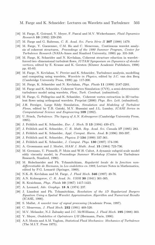
“farge”2001/11/20page 503

�

�

�

�

�

�

�

�


[16] M. Farge, E. Goirand, Y. Meyer, F. Pascal and M.V. Wickerhauser, Fluid DynamicsResearch 10 (1992) 229-250.

[17] M. Farge and G. Rabreau, C. R. Acad. Sci. Paris Serie II 307 (1988) 1479.

[18] M. Farge, Y. Guezennec, C.M. Ho and C. Meneveau, Continuous wavelet analy-sis of coherent structures, Proceedings of the 1990 Summer Program, Center forTurbulence Research (NASA-Ames and Stanford University, 1990) pp. 331-348.

[19] M. Farge, K. Schneider and N. Kevlahan, Coherent structure eduction in wavelet–forced two–dimensional turbulent flows, IUTAM Symposium on Dynamics of slendervortices, edited by E. Krause and K. Gersten (Kluwer Academic Publishers, 1998)pp. 65-83.

[20] M. Farge, N. Kevlahan, V. Perrier and K. Schneider, Turbulence analysis, modellingand computing using wavelets, Wavelets in Physics, edited by J.C. van den Berg(Cambridge University Press, 1999) pp. 117-200.

[21] M. Farge, K. Schneider and N. Kevlahan, Phys. Fluids 11 (1999) 2187-2201.

[22] M. Farge and K. Schneider, Coherent Vortex Simulation (CVS), a semi-deterministicturbulence model using wavelets, Flow, Turb. Combust. (submitted).

[23] M. Farge, G. Pellegrino and K. Schneider, Coherent vortex extraction in 3D turbu-lent flows using orthogonal wavelets. Preprint (2000) Phys. Rev. Lett. (submitted).

[24] J.H. Ferziger, Large Eddy Simulation, Simulation and Modeling of TurbulentFlows, edited by T.B. Gatski, M.Y. Hussaini and J.L. Lumley, ICASE Series inComputational Science and Engineering 109 (1992).

[25] U. Frisch, Turbulence. The legacy of A.N. Kolmogorov (Cambridge University Press,1995).

[26] J. Frohlich and K. Schneider, Eur. J. Mech. B 13 (1994) 439-471.

[27] J. Frohlich and K. Schneider, C. R. Math. Rep. Acad. Sci. Canada 17 (1995) 283.

[28] J. Frohlich and K. Schneider, Appl. Comput. Harm. Anal. 3 (1996) 393-397.

[29] J. Frohlich and K. Schneider, Physica D 134 (1999) 337-361.

[30] J. Frohlich and K. Schneider, J. Comput. Phys. 130 (1997) 174-190.

[31] A. Grossmann and J. Morlet, SIAM J. Math. Anal. 15 (1984) 723-736.

[32] M. Germano, U. Piomelli, P. Moin and W.H. Cabot, A dynamic subgrid scale modeleddy viscosity model, in Proceedings Summer Workshop (Center for TurbulenceResearch, Stanford, 1990).

[33] M. Holschneider and Ph. Tchamitchiam, Regularite locale de la fonction non-differentiable de Riemann, in Les ondelettes en 1989, Lecture Notes in Mathematics,edited by P.G. Lemarie (Springer, 1989).

[34] N.K.-R. Kevlahan and M. Farge, J. Fluid Mech. 346 (1997) 49-76.

[35] A.N. Kolmogorov, C. R. Acad. Sc. USSR 30 (1941) 301-305.

[36] R. Kraichnan, Phys. Fluids 10 (1967) 1417-1423.

[37] A. Leonard, Adv. Geophys. 18 A (1974) 237.

[38] J. Liandrat and Ph. Tchamitchian, Resolution of the 1D Regularized BurgersEquation Using a Spatial Wavelet Approximation Algorithm and Numerical Results(ICASE, 1990).

[39] S. Mallat, A wavelet tour of signal processing (Academic Press, 1997).

[40] C. Meneveau, J. Fluid Mech. 232 (1991) 469-520.

[41] M.V. Melander, N.J. Zabusky and J.C. McWilliams, J. Fluid Mech. 195 (1988) 303.

[42] Y. Meyer, Ondelettes et Operateurs I/II (Hermann, Paris, 1990).

[43] A.S. Monin and A.M. Yaglom, Statistical Fluid Mechanics: Mechanics of Turbulence(The M.I.T. Press 1975).

“farge”2001/11/20page 504

�

�

�

�

�

�

�

�


[44] R. Murenzi, Wavelet transforms associated to the n–dimensional Euclidean Groupwith dilatations, Ph.D. Thesis (UCL, Louvain-la-Neuve, 1989).

[45] J. von Neumann, Recent theories of turbulence, in Collected works (1949–1963) 6,edited by A.H. Taub (Pergamon Press, 1963) p. 437.

[46] V. Perrier and C. Basdevant, Rech. Aerosp. 3 (1989) 53.

[47] V. Perrier, T. Philipovich and C. Basdevant, J. Math. Phys. 36 (1995) 1506-1519.

[48] M. Rogers and R. Moser, Phys. Fluids 6 (1994) 903-923.

[49] P.G. Saffman, Vortex Dynamics (Cambridge University Press, 1972).

[50] K. Schneider and M. Farge, C. R. Acad. Sci. Paris Serie II 325 (1997) 263-270.

[51] K. Schneider, N. Kevlahan and M. Farge, Theoret. Comput. Fluid Dynamics 9(1997) 191-206.

[52] K. Schneider, N. Kevlahan and M. Farge, An adaptive wavelet method comparedto nonlinearly filtered pseudo-spectral methods for two-dimensional turbulence,Advances in Turbulence VII, edited by U. Frisch (Kluwer Academic Publishers,1998) pp. 147-150.

[53] K. Schneider and M. Farge, Wavelet approach for modelling and computing tur-bulence. Lecture Series 1998–05 Advances in turbulence modelling (von KarmanInstitute for Fluid Dynamics, Bruxelles, 1998) 132 pages.

[54] K. Schneider, M. Farge and N. Kevlahan, Intermittency and coherent vortices infully-developed two-dimensional turbulence, Preprint (ICT Universitat Karlsruhe,1999).

[55] K. Schneider and M. Farge, C. R. Acad. Sci. Paris Serie II b (2000) 263-269.

[56] R. Teman, Navier–Stokes equations and nonlinear functional analysis (SIAM,Philadelphia, 1983).

[57] A. Vincent and M. Meneguzzi, J. Fluid Mech. 225 (1991) 1-20.

[58] A. Vincent and M. Meneguzzi, J. Fluid Mech. 258 (1994) 245.

Documents

ANALYSING AND COMPUTING TURBULENT FLOWS USING WAVELETS