JOURNAL OF THE OPTICAL SOCIETV OF AMERICA

Analyses of Yttrium Spectra

ARTHUR B. HooK* AND MATTHEW P. THEKAEKARA

Physics Departmnent, Georgetown University, Washington, D. C. 20007

(Received 10 June 1964)

A near automatic method has been developed for data handling and analysis in atomic spectroscopy. Plate

factors are determined by a least-squares solution of 100 standard lines by using a polynomial up to the fifthdegree. Catalogs of predicted lines are made from known energy level schemes, and classifications of new lines

are suggested. The method has been applied to the visible spectrum of yttrium as produced by electrodelessdischarge tubes. A total of 977 new lines has been measured with an accuracy of 0.005 A in the wavelengthrange 4600 to 6400 A, which is usually masked by oxide bands; 162 of these lines have been classified interms of the known energy level system.

1. INTRODUCTION

THE availability of high-speed digital computersThas added a new degree of freedom to the problemof analyzing atomic spectra. This is the possibility ofgenerating, storing, and handling large sets of data, andis a feature of computers which is potentially as valuableas their ability to perform rapid computations. Thispaper deals with the automation techniques which weredeveloped for (a) data collection, (b) data reduction,and (c) the classification of newly observed spectral linesof yttrium.

The data analysis portion of the problem has beenpartitioned into the three areas mentioned above: col-lection and reduction of data and classification of lines.When combined, these programs accomplish the classi-fication of all new spectral lines which can be identifiedin terms of the known energy level system. The programdoes not, however, make a full search for new spectralterms. The development of such a program is un-necessary since such programs have recently becomeavailable for larger computers through the work of theSpectroscopy section of the National Bureau ofStandards.1-4 Further, Vander Sluis5 has successfullyapplied the digital computer to analysis of Zeemanpatterns.

2. DATA COLLECTION

The very large number of lines on the spectrograms,the accuracy with which their positions can be meas-ured, and the lack of a strict linear relationship betweenthe positions of the lines and their wavelengths made itdesirable to employ time-saving devices for measure-ment and data reduction.

The source was an electrodeless discharge tube, con-taining yttrium salts, of a type which has been described

* Present address: Engineering Research and DevelopmentLaboratories, Fort Belvoir, Virginia.

1 W. R. Bozman, J. Opt. Soc. Am. 44, 824 (A) (1954).2 K. G. Kessler, S. B. Prusch, and J. A. Stegun, Bull. Am. Phys.

Soc. 1, 22 (1956).3 K. G. Kessler, S. B. Prusch, and J. A. Stegun, J. Opt. Soc. Am.

46, 1043 (1956).4 C. D. Coleman and W. R. Bozman, J. Opt. Soc. Am. 49, 511

(A) (1959).1 K. L. Vander Sluis, J. Opt. Soc. Am. 49, 944 (1959).

previously.6 -9 The spectrum was photographed with a15 000 lines/in., 21-ft radius grating in a Wadsworthmounting. An image of the discharge tube is focused ona narrow vertical slit, about 30,p in width. Although thedispersion is approximately constant, it is necessary tocalibrate the plates by reference to wavelengths of awell-known spectrum like that of iron.

Over 100 plates were photographed, in the initialstages of this research, on the spectrograph located inthe basement of the Georgetown College Observatory.Later, a similar spectrograph at the National Bureauof Standards was used to prepare about 15 plates. Theavailability of plates from two entirely different gratingswas helpful for the elimination of ghost lines. The timeof exposure varied from 3 to 10 min. In general, twodifferent sets of exposures were made on each plate-oneset with a short exposure to give sharp images of thestrong lines and another set with longer exposure to giveall the weak lines, avoiding, however, the fogging dueto the continuum. For each of the two sets, four spectra(1) FeI2 , (2) Y13 , (3) YI3 and FeI2 , and (4) FeI2 werephotographed one below the other. The third set wasmade using a discharge tube which contained smallamounts of FeI2 in the Y13. With these, the iodine linescould be distinguished from the comparison spectrumof iron and the unknown yttrium spectrum. Kodak spec-troscopic plates of emulsion types 0, D, and F providedthe required spectral sensitivity for the wavelengthregion under consideration.

Some of the early measurements and data reductionof the plates were made with the comparator, tele-cordex, and computer of the Georgetown CollegeObservatory by use of techniques similar to those de-scribed by Wilson and Thekaekara.10 In the later stagesof the work, as photographic plates of greater spectralpurity and more dense lines became available, it wasnecessary to develop a more fully automatic program.A David Mann measuring comparator was modified by

I C. H. Corliss, W. R. Bozman, and F. 0. Westfall, J. Opt. Soc.Am. 43, 398 (1953).

7 W. E. Howe, J. Opt. Soc. Am. 48, 28 (1958).8 A. Wardakee, J. Opt. Soc. Am. 54, 460 (1964).I J. F. G-uiliani and M. P. Thekaekara, J. Opt. Soc. Am. 54,

460 (1964).10 C. M. Wilson and M. P. Thekaekara, J. Opt. Soc. Am. 51,

289 (1961).

1445

DECEIM1ER 0964VOLUiME 54, NtJMBEk t2

A. B. HOOK AND MX. P. THEKAEKARA

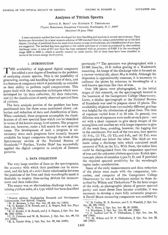
FIG. 1. Plate calibi

addition of a magneequally spaced sign;that is, one pulsecarriage.

As the plate carmicroscope, its posiaccumulator. Additestimated intensity,spectral line is insetsequence of code nmof a key punch boarby means of a foot seight-channel punc.taneously printed onthrough an electrictions, the line-measian average rate of o2-5 u. At this measu:a single pass over a4-5 h. Since a reversform a complete setgiven spectrum, abospent in measuringmeasurements are uand four sets of platrange, the magnitudeautomation. Withouwould be increased r

A total of severalcontaining over 10 (than 30 spectrograirwhich the accumulaplate is fixed by thereference spectrum.set at a wavelengthsorption limit of airsetting of the gratingx-value on all plates;out the iron standasystem has not pickduring the 4 or 5 h r

I'lo o ~

-20

o-,40

4

II

1446 Vol. 54

1 |urements, the crosshair is reset on the reference lineagain at the end of each run to check its reading againstthe initial accumulator setting.

3. WAVELENGTH COMPUTATION

0° > ° 9The central problem in the application of automation

,to spectroscopic data reduction is that of setting up a

computer routine that will accurately transform themeasured positions of the lines to their wavelengthswith respect to the iron standard.

In general, the transformation from position x towavelength X can be accomplished through an extension

' 0 $of the procedures used by Wilson and Thekaekara' 0 andearlier by Dieke, Dimock, and Crosswhite.1" A recent

ration curve as plotted automatically. compilation by Crosswhite'2 was used for wavelengthcalibration.

!tic read-out head, which emits 1000 The method is graphically illustrated in Fig. 1, whichil pulses per revolution of the screw, shows the results of a superimposed dual plot illustrat-for 1 g of movement of the plate ing the data scatter about the plate correction function.

This plot reveals the importance of establishing a non-

riage is moved under the viewing linear correction base for some cases. It also facilitatestion is registered on a seven-digit correction for: (1) misidentified lines, (2) poorly meas-

tional information concerninnd the ured lines, and (3) bad wavelength standards; the cards

identification, and character of the for those lines which lie too far off the plate correction

-ted into the system by punching a curve may be simply removed and discarded. If too

imbers into the first three columns many such corrections are made, the least-squares

d. The read-out system is triggered fitting may be repeated, without those cards, to obtain

witch. The data are recorded on an better values of the coefficients, and to establish anhed paper tape, and are simul- even better plate correction function. Normally, this is

a continuous sheet of paper passing not required.typewriter. Under normal condi- The wavelengths of lines other than those of iron are

iring sequence can be continued at calculated by using the transformation equation and byne line per 10 sec with precision of applying the plate correction function. The wave-ring rate, the time required to make numbers are calculated by using the Edl6n dispersion10-in. plate of about 500-A range is formula for the refractive index of standard air.se run is always required in order to The computational procedure is repeated for eachof averaged measurements for any measured set of data until a sufficient number of in-ut ten or more hours are normally dependent values Xa and a-, have been obtained. The

uach plate. Since 5-15 independent average values for each line are determined.

sually made for each spectral line.s are required to cover the 2000-A 4. CATALOGS OF PREDICTED LINES

of the task is apparent-even with A program was written for the RCA 301A computert automation, the measuring time to generate three sets of spectral catalogs for all possibleMnother order of magnitude. odd-even, even-odd transitions between 2000 andhundred data sheets was obtained, 10 000 A for neutral yttrium, singly ionized yttrium,)00 line measurements from more and doubly ionized yttrium. The programming in-is. The range of measured values volved only isolating the levels of opposite parity intotor passes through on any given separate sets, and applying the selection rules for J,associated wavelength range of the namely AJ=0 or dri, but not J=0 to J=0.The zero reference of the scale was Since the coupling scheme in yttrium is not strictlyroughly corresponding to the ab- Russell-Saunders, it was decided not to apply the selec-at 1900 A. Therefore, for a given tion rule prohibiting intercombination between multi-

each line has practically the same . 1 G. H. Dicke, G. H. Dimock, and H. M. Crosswhite, J. Opt.this facilitates the task of picking Soc. Am. 46, 456 (1956).

rds. To ensure that the read-out 12 H. M. Crosswhite, Johns Hopkins Spectroscopic ReportNo. 13 (August 1958, unpublished). A partial listing of the linesled up or dropped a few microns is also available in American Institute of Physics Handbook

required to complete a set of meas- (McGraw-Hill Book Company, Inc., New York, 1957), pp. 7-89.

December 1964 ANALYSES OF YTTRIUM SPECTRA

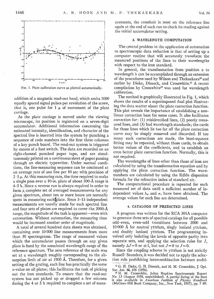
TABLE I. Newly classified lines of yttrium.

Wavelength WavenumberX (A) ,-(cm-,)

4639.044665.544680.094694.5224695.7944704.8774721.2754727.9734732.2924732.7444750.3374758.7224766.0644776.9344779.4954788.6674814.7204822.2824825.2 174833.0884848.8294850.6724854.9814867.7954870.0914879.1694886.9244896.11049 11.5544923.7624925.1464928.3764935.0674963.4854981.9815002.4535004.4355009.1165025.1615040.4855043.1645043.3895096.8495096.9875098.5725099.5295107.8585109.1495119.5735122.5575130.0765 141.9805154.3575177.6195184.5945186.5155202.3945205.0225205.1735210.75552 19.598522 1.0295231.5845232.1125254.07 15258.4785265.6435268.254527 1.8155277.0425278.7355286.7175289.330

21 550.1 O21 427.74321 361.13221 295.46421 289.99821 248.59621 174.79621144.79721 128.50021 123.48621 045.25121 008.17220 975.80820 928.07720 916.86520 876.79920 763.83820 731.28720 718.66720 684.92820 617.77720 609.94520 591.65120 537.44520 527.76820 489.57320 457.09020 418.68020 354.47520 303.00820 298.30320 284.99920 257.49820 141.51620 066.73719 984.61719 976.70519 958.03719 894.31319 833.83219 823.32019 822.41319 614.49919 613.96519 607.86719 604.18919 572.22319 567.28019 527.43919 516.06319 487.46119 442.34319 395.66019 308.51919 282.54219 275.40119 216.56919 206.86919 206.31219 185.73719 153.23219 147.98219 109.35319 107.42219 027.56719 011.62118 985.74918 976.34118 963.52418 944.74118 938.66318 910.07018 900.727

Classification

22233112

3

24

3

11

20

3

0

241

0

1

41

2301

3021

020

41

3

434

2022

30230

0323

0

31

0

1

23

Wavelength Wavenumberx (A) e(cm-')

z 2F'5/2-g 2D5/2

z 4P 1/2-f 4p3 /2

z 4F, 7/2- (1) 5/2y 2p

0

11 2/f 2P./

2

a 4Pl/2-w 2D06/2

y 2p1

/2.-f p1/2

z 4F61/2-f 2D3/2

y 2F52/2-(3) 7/2

a 2F5/2-W 2DW°/a 4P 3 /2-W wD 2b 2D1/2-y 'P°l/2

Z 2D 1 /2- (1)1/2

a 4P6/2-w 2D0

21

z 2D3/2- (1)5/2

y 2D°6/2- (3) 7/2

y 2D°312-h 4D6/

y 2F°7/2- (3) 7/2

z 2P°l/2-b 4P1/2

z 4FO7/2-f 2D5 /2y 2F°5/2-h 4D7/2

z 2p°a/2-b 4PI/2

z 4P0

5/2 -e 4F7/2

b 2Dl/2-Z 4S'S/ 2z 4P°3/2-e 4F6/2

y 2p°3/2-h 'Db/,

y 2F°l/2-h 4D5/2y 2D'l/2-h 4D7/2

z 4P21/2-e 4F1/2

z 2D0

5/2-f 2D3

y 2FO7/2-h 4D7/2Z 4P°5/2-e 4Fl/2Z 2D°3/ 2 -f 2D 1 /2

z 4D°5/2-(1)5/2

b 2D3/2--X 4D%/2

b 2D1 /2-x 4D3

5/2z 4D1/2 -f2D3 /2

b 2D6/2-X xD 2z 4D°7/2- (1) 5/2

b 2D1 ./2 -x 4D2S

z 4D2

1/2-f 2D5/2z 4D°3/2-f 2D3/

b 2

D1/2-X 4D0

1/2

z 4D0

5 /2-f 2D6/2z 4P°5/2-e 4G7

z 4P03/2-e 4G5/2

z 4D2

5 /2-f 2D3 /2

z 4F°3/2-e 4Pl/2Z 4P°I/2-f 4D/2

z 4P2

1 /2_f 4DZ 4PO3/2-f 4D/2

z 4P°5/2-e 4G6

z 4PO3/2-f 4D/2

z 4P56/2-f 4Dlp2

z 4F03/2-e 2D5/2

z 4F0

3/2-e 2D 2 /2

z 4F°5/2-e 4P5/2

a 45P/2-Z2S'2/2

z 4

F°a/2-e 4P3/2

y 2

D0

3/2-f 4F6/2

y 2F

21/2-f 4F7/2

y 2F0

7/2-g 4F5/2

a 2D3/2-Z 4P50/2

a 4P3/2-z 2S21 /2

a 2G7/2-w 2F07/2

a 2D 3 /2-Z 4P53/2

z 4F0

5/2-e 2D 5/2

z 4F0

5/2-e 2D3 /2

a 2D3/2-Z 4P523/

a 2G7/2-y 4P2

5 /2y

2P

01/2-g

2SI/2

y 2D'i22-g 2D5/2

z 4F°s/2-e 4P3/2a 2G7/2-w 2F°5/2

5291.3975345.2365356.35()5377.4005377.9575381.248538 1.4795382.3635387.9995389.0 105396.7975401.8785404.7 145414.8655420.2595422.1045440.6425456.0235466.2255476.8275500.5545502.1405519.8825526.4495532.5665539.1785544.5125544.6 145545.158555 1.9255558.0245567.3895573.0345573.6965579.5545593.4705596.9755601.0865604.5745615.8885617 .8005627.3115634.1995634.7065641.7745664.2595669.5585708.3965714.9555727.2445729.2565740.6255743.3945747.8435757.6035763.9425784.3775788.3745790.3285801.0935807.3935820.0165839.3035844.1455849.1285864.8125875.2 125898.0 115907.1855926.4215934.7515935.175602 7.587

1447

I Classification

18 893.34418 703.04718 664.23818 591.06718 589.25618 577.88418 577.04218 574.03518 554.60918 551.12718 524.35718 506.93418 497.22218 462.54918 444.17718 437.90218 375.07918 323.27718 289.99418 253.67618 174.93818 169.70018 111.29918 089.77618 069.77518 048.20818 030.84518 030.51418 028.74418 006.76917 987.01217 956.75317 938.56517 936.43517 917.60517 873.02817 861.83517 848.72317 837.61917 801.68417 795.62417 765.54917 743.82717 742.23317 720.00317 649.62617 633.16817 513.19917 493.09817 455.56317 449.43617 414.87817 406.48017 393.00717 363.52517 344.42917 283.15317 271.22117 265.39217 233.35417 214.65717 177.32317 120.58517 106.40t17 091.82617 046.12417 015.94816 950.17216 923.84616 868.91616 845.24116 844.03716 585.794

00

2002001

02223203I

32203

22

63022340310010

2

0I

1

200

0

4

22

303321

2033

1

21

21001

3

z 4F

23/2-e 2P3 /

2

a 2F3/-X 2Fx 7/2

z 4F'312-e 2P e2

y 2D01 /2 -f 4F5/1

y 2

P'3/2-g 2D5/2

a 'P3/2-x 2D0

1 /2y 2FO6/2-f 4F

3/2

y 4F'1

/2-g 4P6/2

y 2D'3/2-P Sl/2

y 2

F01/2-g 2D

5/2

y 2D2

312-g 2D 21 2

z 4F'512-e 4D7/2

a 2Dz/2-Z 4p0

1 1 2

z 4F'3/2-e 4D5/2b 2D2 /2-z 2S°1/2

y 2FO7/2 -f14F/2

z 2D'3/2-e 4P/1 2

y 2D'5/,2-g 2D5/-2

z 4F

23/2-e 4Dl/2

b 2D3/2-x 2D0

1 /2y 2p%3/2-g 2D

2/2

x 2P2

1 1 2-f 2p3/2

z 2D°3/2-e 2D6/2

z 2D0

1 /2-e 4P3 / 2

a 2P3/2-y 4P°o/,z 2F'7/2-e 4F9/2a 2F5/2-y 4D

01 1 2

a 3PI-y 3pJo

a 4P1 /2--y 4D°1 /2

a 2P3/2-w 2F°6/2y2Pi

1/2-f 2Si/2

y P2

l,/2-g 2D3

/2

a 2F5/2-y 4Da/2

a 'P3/2-y 4D°3/2

Z 2F°5/2-e 4F3/2

a 2P3/2-w 2P 1 1/2a

2G9/2-X 4Dx7/2

a 2

G7/2-X 4Dx7/2a 2P3/2-w 2p°2 /2a 2PI/2-y 4Po1 /2

z 4D°i/2-e 2DeZ2

z 2D°3/2-e 4PI/2

a 2F7/2-X XF'5/2

a 2P3/2-y 4PO3/2

z 4D'112-e 4P3/2

Z 2F°7/2-e 4Fe/2

a 2p1 /2-y 4P°1/2

a 2Pu/2-z 4S13/2a 2F7/2-y 4D°5/2

b 2D5/2-y 4D2

7/2b 2D1 /2-X 2F x/2

z 4D'5/2-e 2D

3/2

z 4D0

1/2-e 2P3e2

z 4P2

3 /2-f 2D3 /2

b 2D 3/2-y 4D6/2a 2P3/2-z 4S'2/2

z 4P°5/2-f 2DDI/2b 2D3 /2-y 4D°3/2

z 2Df3/2-e 4De/2

z 2F2

5/2-e 4G7/2

a 2Pl/2-w 2D2

3 /2

Z 4D'112-e 2PI/2

z 4F°6/2-b 4p5

/2

b 2D5/2-y 4D'3 /2

Z 2DO3/2-e 4De/2a 2P3 /2-w 2D'312

z 4D0I/2-e 2Pe/2

z 2F2

7/2-f 4D7/2

X 2P2

1/2-h 4D3/1

x 2P°3/2-h 4D6/,z 4F°5/2-b 4p2 /2

x 2P0

3.2- (2) 1/2,3/.

a 2D5/2-Z D7

A. B. HOOK AND 1M. P. THEKAERKAA R A

TABLE I (continued)

Wavelengthx(A)

6028.8126030.1266082.5726083.7776133.1626163 .4096178.0956222.2386234.0996238.5456269.8816314.8116319,7916321.1476339.2296339.7 716347.3356353.3806373.358

\Vav \enurnb llera(cm -l)

16 582.42616 578.81216 435.863164132.60916 300.29216 220.29716 181.74416 066.94416 036.37516 024.94815 944.85715 831.41115 818.93415 815.54215 770.43015 769.10415 750.29015 735.30415 685.981

I Classificationl

1 a 2F5/2-y 4pF07

03

3003

3

02

00

30

a 'PI12-X 4D'Da 2D3y,2z 'D

0,1 2

a 'Psj2-y 4JF'7/

Z 2D'3/2-b 4P5/2

a 2Fsp2-y 4FW'v

a 2D5/2-z 4D%1 ,y 2 p312f4Pb/2

z SD0

,/2-b 'Pi/2Z 1D'3i2-b 4P3,2z 2D°312-b 4PI/2

X 2pO,2,-g 2S,,2

a 2F7/2-y 4F'6/2Y ID°612-J4PS12

Z 4D°3/2-b 4P52

b 2

Ds/2-y 4F'71a 2G7/2-x 2DO5/2

b 'D312-y 'F'5j2

plet terms. Meggers and Russell" had observed inter-system combinations in 27% of the lines which theyclassified, and it was very likely that more would befound, since many weaker transitions are usually ob-served with the electrodeless lamp. Lines arising frommagnetic dipole and electric quadrupole transitionswere not considered, since there was no reason to expectsuch lines under the conditions prevailing in an elec-trodeless lamp.

(A) The energy level designations and wavenumbersfor the even and odd states of an atomic system arekey-punched and compiled in two separate card decks.The term values are taken from Moore.'4 One of thecard stacks, say the odd, is then arranged in order ofincreasing wavenumber and is read into the computerstorage.

(B) The Pith even level Tn is then chosen from theeven stack, starting with the lowest term value whichis the a 2D,1 state of Y i, with T,= 0.00, and it is com-pared successively with each of the odd terms. The dif-ference in term values and the corresponding wave-lengths are calculated, provided the selection rule for Jholds, and the wavelength is between 2000 and 10 000A. The wavelengths are arranged in sequence and theresults are printed out.

The complete predicted catalog for the region 2000-10 000 A contains a listing of 1594 (Y i), 430 (Y ii),and 13 (Y in) possible transitions odd to even and evento odd. Of these, a total of 549 (Y I) and 32 (Y II)possible transitions were in the spectral region, 4596-6424 A, covered in this present study.

This program for compiling a predicted catalog hasbeen applied also to the first spectrum of titanium.Compared to neutral yttrium which has 79 even and 66odd known levels, neutral titanium has 166 even and

13 W. F. Meggers and H. N. Russell, J. Res. Nat]. Bur. Std. 2,733 (1929).

I" C. E. Moore, Natl. Bur. Std. Circ. No. 467, 196-(1952).

208 odd levels, and gives nearly 9500 predicted tran-sitions. The application of this list for the classificationof over 1000 new lines in the first spectrum of titaniumis reported elsewhere.1 5 1 6

5. THE SPECTRA OF YTTRIUM

The analysis of the yttrium spectra has remained ina state of partial completion since the extensive workof Meggers and Russell"3 in 1929. Their listing of termvalues was based on the wavelength measurements of448 lines of Y i and 223 lines of Y ii made in earlieryears, mainlx by King and Carter,'7 Meggers,' 8 Kiess,' 9

and Meggers and Moore.20 Thirty-nine new levels ofyttrium iI, based on additional lines observed with ahollow cathode light source, were provisionally sug-gested by Ho and Sawyer2 ' in 1937. Since these levelswere not fitted into the existing term array of Y ii, theywere omitted in Moore's compilation of atomic energylevels, pending further confirmation of the newly ob-served lines by use of instruments of higher resolutionand greater dispersion.

With the exception of the hollow cathode light sourceused by Ho and Sawyer, all earlier work has been donewith the conventional free-burning arc or high-voltagealternating current spark. These hot arc sources ofradiation have done an effective job of dissociating re-fractory compounds and of exciting their atomic andionic spectra. However, the high temperatures, appre-ciable pressures, and strong electric fields which char-acterize these light sources lead to excessive broadeningof the emitted spectral lines. The electrodeless dischargetube offers several advantages: The source is con-siderably brighter, the lines are relatively sharp, aspectrum of high purity can be obtained, and the tubehas a fairly long lifetime.

For a study of the spectra of yttrium, the electrode-less discharge tube is of special significance. In thespectrum of the free-burning arc, there are two yttriumoxide band systems22 which obscure large portions of thevisible atomic spectrum. These bands are due to the

2 (ground state) transitions in the range 4650to 5580 A and the 2f + 2 (ground state) transitionsin the range 5580 to 6500 A.

The present investigations of the yttrium spectra wasundertaken to map out and to analyze the wavelength

15 H. W. Banks, "First Spectrum of Titanium from 6000 A to3000 A," Doctoral dissertation, Georgetown University, Washing-ton. D. C. (1961).

"W. R. Bozman, "The Spectrum of Titanium from 6000 A to9000 A," Master's thesis, Georgetown University, Washington,D. C. (1961).

"A. S. King and E. Carter, Astrophys. J. 65, 86 (1927).8 W. F. Meggers, J. Wash. Acad. Sci. 14, 427 (1924).

1XV. F. Meggers and C. C. Kiess, J. Opt. Soc. Am. 12, 417(1926).

'W. F. Meggers and C. E. Moore, J. Wash. Acad. Sci. 15, 207(1925).

"1 I-djen Ho and R. A. Sawyer, Phys. Rev. 51, 1202A (1937).21 R. W. B. Pearse and A. G. Gaydon, The Identification of

3Iolecidar Spectra (John Wiley & Sons, Inc., New York, 1950),p. 246.

1448 Vol. 54

December 1964 ANALYSES OF YTTRIUM SPECTRA

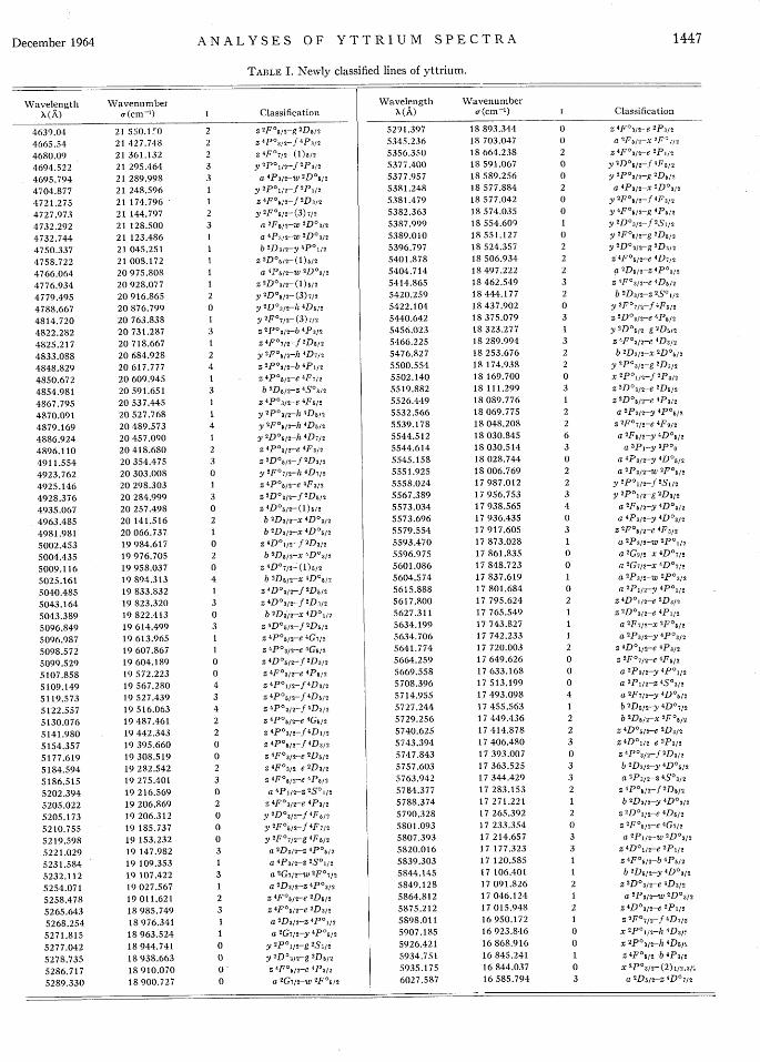
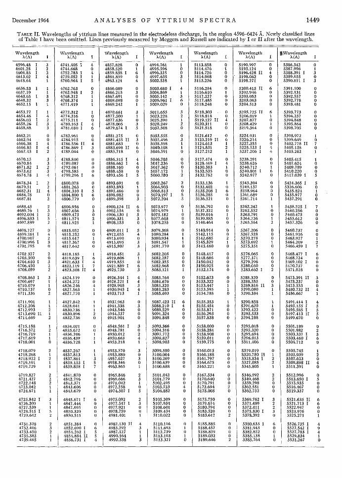
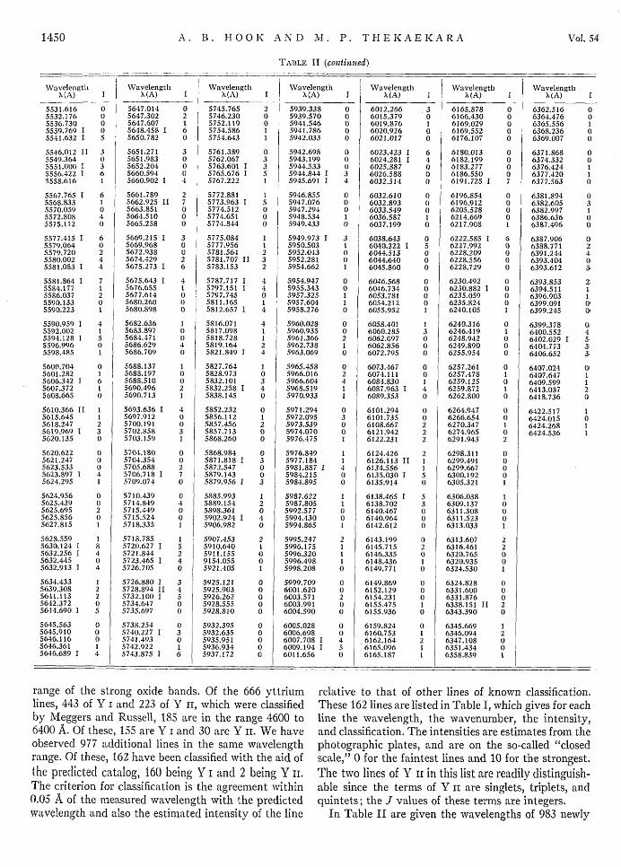
TABLE II. Wavelengths of yttrium lines measured in the electrodeless discharge, in the region 4596-6424 A. Newly classified linesof Table I have been omitted. Lines previously measured by Meggers and Russell are indicated by I or II after the wavelength.

Wavelength Wavelength Wavelength WavelengthX (A) I X (A) I X(A) I ?(A) I

4596.48 1 3 4741.405 1 4 4857.828 0 4994.761 14601.28 I 2 4744.668 0 4858.520 1 4995.596 04604.85 I 2 4752.783 I 4 4859.838 1 6 4996.335 04613.02 I 4 4759.052 1 1 4861.859 0 4997.635 34618.64 1 4760.964 I 5 4863.121 4 5002.538 1

4636.53 1 1 4762.763 0 4866.089 0 5003.680 I 44637.19 1 4762.948 I 2 4866.215 3 5004.869 14643.65 I 3 4768.312 1 4867.691 0 5005.142 34648.32 3 4768.374 1 4869.098 0 5006.961 1 64652.15 1 1 4771.419 1 4869.242 1 5009.029 0

4653.77 I 1 4772.312 1 4870.661 3 5011.655 34654.46 I 4 4774.316 0 4877.500 1 5023.228 24656.03 I 2 4775.211 0 4877.636 0 5025.390 14658.26 1 3 4780.163 I 4 4878.006 3 5028.249 24658.88 3 4781.030 I 6 4879.674 I 5 5032.508 0

4662.21 0 4782.961 0 4881.275 0 5033.555 04662.94 0 4784.915 0 4881.455 II 3 5035.496 34666.38 I 4 4786.556 II 4 4881.683 0 5038.598 14666.85 I 4 4786.869 I 3 4883.698 II 6 5040.108 14667.45 I 2 4788.044 0 4885.718 0 5046.591 0

4670.15 3 4788.840 0 4886.315 I 4 5046.703 04670.84 3 4789.087 0 4886.662 I 4 5047.236 04671.82 I 2 4792.061 0 4888.160 0 5047.362 04673.62 3 4798.585 0 4888.458 0 5057.172 14674.78 I 4 I 4799.296 I 6 4893.456 I 5 5060.780 2

4678.34 I 2 4800.078 0 4893.691 0 5062.267 24679.51 2 4801.263 0 4893.893 1 5064.903 04682.31 II 4 4804.310 1 5 4895.466 0 5068.813 04684.78 0 4804.800 1 6 4898.082 0 5070.197 I 54687.81 2 4806.779 0 4899.398 3 5072.204 5

4688.43 2 4806.956 0 4900.124 II 6 5073.977 04689.76 1 3 4807.656 3 4902.154 0 5074.979 14692.004 1 2 4809.473 0 4906.130 1 5 5075.182 04696.833 I 5 4811.574 2 4906.331 3 5077.603 04697.889 2 4811.925 1 4908.153 0 5078.255 0

4698.727 0 4815.052 0 4909.011 I 5 5079.368 04699.261 I 4 4815.252 0 4912.055 4 5080.284 14700.907 2 4815.617 1 4913.690 0 5080.934 14700.996 1 3 4817.367 0 4915.095 3 5081.547 14701.795 0 4817.642 0 4915.807 3 5081.770 0

4702 327 2 4818.185 1 4918.451 3 5082.208 04703.300 0 4819.639 I 6 4919.606 1 5082.287 04704.640 I 3 4821.633 I 4 4919.855 0 5082.355 04706.450 2 4822.119 1 7 4921.889 I 6 5082.968 04708.059 2 4823.308 II 4 4925.730 3 5083.121 1

4708.863 I 3 4824.119 0 4926.344 1 4 5083.764 04709.697 1 4824.272 0 4928.221 1 4 5084.676 04710.079 1 4826.246 4 4928.905 3 5085.320 04710.737 0 4827.563 1 4930.945 I 4 5085.283 04711.336 2 4827.770 1 4933.713 1 5085.693 0

4711.901 1 4827.842 1 4937.963 0 5087.423 II 64712.206 1 4828.041 1 4941.338 3 5088.210 1 44712.993 2 4830.736 1 4943.546 0 5089.529 04713.690 II 1 4830.896 2 4944.337 0 5091.324 04714.669 2 4832.736 0 4945.901 0 5091.848 0

4715.188 1 4834.021 0 4848.561 I 3 5093.366 04716.372 2 4835.672 0 4948.781 0 5094.316 04716.719 1 4836.206 1 4950.012 2 5097.772 04717.619 1 4836.439 1 4950.663 4 5098.827 04718.001 0 4836.728 1 4953.218 1 5098.903 0

4718.079 2 4837.267 1 4953.570 3 5099.590 04718.268 1 4837.813 1 4953.880 0 5100.064 04718.922 I 2 4837.861 3 4957.627 3 5100.269 04719.101 1 4839.153 1 5 4958.346 0 5100.439 04719.729 1 4839.858 I 7 4963.865 1 5100.688 0

4719.827 2 4841.870 0 4965.846 2 5101.042 04721.427 2 4842.796 0 4969.666 3 5101.779 04722.148 2 4843.371 0 4971.042 1 5102.495 04723.042 1 4843.606 0 4972.258 0 5103.723 44724.671 1 4843.679 0 4974.307 1 5 5104.882 0

4725.842 I 3 4845.671 I 6 4975.092 2 5105.209 04726.309 1 4847.444 0 4977.547 1 3 5107.934 04727.539 1 4847.695 0 4977.921 0 5108.601 04728.515 I 5 4850.320 0 4978.759 u 5109.434 04729.642 2 4850.515 0 4981.401 1 5110.022 0

4731.328 2 4851.384 0 4982.130 IT 4 5110.116 04732.406 3 4852.690 I 6 4983.292 3 5111.693 14733.450 2 4854.262 I 5 4987.127 1 5112.739 04735.383 1 4854.884 II 5 4990.164 1 5113.103 14739.465 1 4856.731 I 4 4992.338 3 5113.321 0

Wavelength WavelengthX (A) I X (A) I

5113.858 0 5190.997 05114.476 1 5193.124 05114.726 0 5196.428 II 45114.968 0 ' 5198.062 05115.236 0 5198.271 0

5116.284 0 5200.415 II 65116.610 1 5202.946 05117.227 0 5203.053 05117.485 0 5203.063 05118.248 0 5204.513 0

5118.303 0 5205.725 II 65118.818 0 5206.019 15119.127 II 4 5207.877 05120.311 0 5208.429 15121.518 0 5219.364 0

5121.612 0 5224.931 05123.219 II 6 5226.214 05 124.613 1 5227.355 05124.831 2 5228.533 1 45127.212 1 5237.206 I 4

5127.474 0 5238.291 05128.469 I 4 5238.626 05130.383 1 5240.712 15132.535 0 5240.801 1 65132.782 0 5242.977 0

5133.136 1 5243.304 05133.402 0 5249.137 05135.208 I 6 5258.964 05136.285 0 5261.689 05136.521 0 5261.714 1

5136.792 0 5262.242 15137.322 0 5262.552 05139.016 1 5263.791 05139.885 0 5264.226 15140.464 0 5265.564 2

5140.914 0 5267.206 05142.115 0 5267.528 05142.685 2 5270.278 05145.329 1 5273.692 15145.460 0 5275.351 0

5148.417 0 5276.065 05148.686 0 5277.371 05150.042 0 5279.296 05150.925 0 5280.060 05152.174 0 5283.662 I 2

5152.673 0 5288.320 05153.322 0 5288.555 05153.447 1 5289.816 II 35153.595 1 5290.080 15154.788 0 5290.384 1

5155.353 1 5290.858 15155.454 0 5291.620 15155.871 0 5292.422 05156.293 0 5293.533 05157.838 0 5294.288 0

5158.000 0 5295.018 05158.284 0 5295.320 05158.908 0 5295.694 05159.011 0 5296.013 05159.775 0 5311.406 0

5160.015 0 5319.019 05160.188 0 5320.780 II 15161.797 0 5325.834 1 25164.675 0 5327.085 25165.221 0 5345.805 1

5167.334 0 5346.992 25170.640 0 5349.468 25170.791 0 5359.298 05172.694 2 5362.551 05175.008 0 5362.752 0

5175.750 0 5369.762 I 35179.674 0 5371.489 25180.794 0 5372.411 25183.520 0 5375.830 I 35183.612 2 5378.392 0

5185.885 0 5380.633 I 65188.457 0 5381.943 05188.859 0 5382.852 05189.032 0 5385.138 15189.646 2 5385.764 0

1,WavelengthX(A) I

5386.342 05387.996 15388.391 1 35389.655 05390.811 I 3

5391.100 05392.131 05392.557 05392.778 05393.481 0

5393.773 05394.237 05394.848 05395.864 05398.705 0

5398.972 15399.649 05402.778 II 75405.138 05405.262 1

5405.415 15407.624 05409.789 05410.220 05417.039 I S

5424.365 I S5326.606 05435.824 15435.977 05437.291 0

5438.225 I 75440.256 05440.475 05455.612 05457.326 0

5460.737 05461.916 05463.927 15464.209 25466.459 I 7

5468.477 I 65468.724 05469.102 I 05470.737 05471.028 0

5473.391 11 35475.237 05475.553 05480.732 II 45486.667 1

5491.414 I 45493.155 1 55495.585 I 55497.413 II 55499.670 0

5501.189 05501.982 25503.337 I 35503.460 I 65504.712 0

5505.745 15505.939 25507.623 05509.898 II 45511.391 0

5512.996 05513.650 I 55515.935 05516.467 05519.337 0

5521.635 II 65521.713 I 65522.947 05523.976 05525.271 1

5526.735 1 45527.542 1 95527.783 I 45529.834 15531.267 0

1449

- --

A. B. HOOK AND IM. P. THEKAEKARA

TABLE II (continned)

WavelengthX (A) I

5531.6165532.1765536.7305539.769 I5541.632 I

5546.012 1 I5549.3645551.00(1 15556.422 15558.616

5567.765 15568.8335570.0595572.8085575.112

5577.415 I5579.0645579.7205580.0025581.083 1

5581.864 I5584.1775586.0375590.1335590.223

5590.959 I5592.0025594.128 15596.9965598.485

5600.7045601.2825606.342 I5607.3 725608.665

5610.366 II5615.6455618.2475619.969 15620.135

5620.6225621.2475623.5335623.897 15624.295

5624.9565625.4395625.6955625.8565627,815

5628.5595630.124 I5632.256 I5632.4455632.913 1

5634.4335639.3085641.1135642.3725644.690 1

5645.5635645.9105646.1165646.3615646.689 I

00005

3036

1

6

040

60244

7

1

20

4

1

5

1)

0

6

0

230

0

()

0

4

1

002

84

(1

2205

000

4

5816.0715817.0985818.7285819.1645821.849 1

5827.7645828.9735832.1015832.258 I5838.145

5852.2325856.1125857.4565857.7 135868.260

5868.9845871.818 15872.5475879.1435879.956 1

5885.9935889.1545898.3615902.924 I5906.982

5907.4535910.6405911.1559154.055592 1.405

5925.1215925.9035926.2625928.5555928.810

5932.3955932.6355935.9515936.9345937.172

2040

2

00

00

000

00

000

Wavelength WavelengthX (A) I X (A) I

5647.014 0 5745.765 25647.302 2 5746.230 05647.607 1 5752.119 05648.458 I 6 5754.586 15650.782 0 5754.643 1

5651.271 3 5761.389 05651.983 0 5762.067 35652.204 0 5763.601 1 35660.594 0 5765.676 1 55660.902 1 4 5767.222 1

5661.789 2 5772.881 15662.925 I1 7 5773.963 1 55663.851 0 5774.512 05664.510 0 ' 5774.651 05665.258 0 5774.844 0

5669.215 I 3 5775.084 15669.968 0 5777.956 15672.938 0 5781.564 25674.429 2 5781.707 II 35675.273 I 6 5783.153 2

5675.643 I 4 5787.717 1 45676.655 1 5797.151 1 45677.614 0 5797.745 05680.260 (1 5811.165 15680.898 0 5812.657 I 4

Wavelength Wavelength? (A) I X (A) I

00000

WavelengtlX(A)

5939.3385939.5705941.5465941.7865942.033

5942.6985943.1995944.5335944.844 I5945.691 I

5946.8555947.0765947.2945948.5345949.433

5949.973 15950.5035952.0435952.2815954.662

5954.9475955.3435957.325595 7.6045958.276

5960.0285960.9355961.3665962.7385963.069

5965.4585966.0165966.6045968.5195970.933

597 1.2945972.0955973.5395974.0705976.475

5976.8495977.1845981.887 15984.2155984.895

5987.6225987 .8055992.5775994.4305994.865

5995.2475996.1755996.3205996.4985998.208

5999.7096001.6206003.5716003.9916004.590

6005.0286006.6986007.708 16009.194 I6011.656

00034

0001°0

3

10

00

0

0110

2

0

0214

0

3

4

00

00

0

0

0

200

0

0450

0

211

10

452

range of the strong oxide bands. Of the 666 yttriumlines, 443 of Y i and 223 of Y ii, which were classifiedby Meggers and Russell, 185 are in the range 4600 to6400 A. Of these, 155 are Y i and 30 are Y ii. We haveobserved 977 additional lines in the same wavelengthrange. Of these, 162 have been classified with the aid ofthe predicted catalog, 160 being Y i and 2 being Y ii.The criterion for classification is the agreement within0.05 A of the measured wavelength with the predictedwavelength and also the estimated intensity of the line

relative to that of other lines of known classification.These 162 lines are listed in Table I, which gives for eachline the wavelength, the wavenumber, the intensity,and classification. The intensities are estimates from thephotographic plates, and are on the so-called "closedscale," 0 for the faintest lines and 10 for the strongest.The two lines of Y I" in this list are readily distinguish-able since the terms of Y ii are singlets, triplets, andquintets; the J values of these terms are integers.

In Table II are given the wavelengths of 983 newly

1450 Vol. 54

5682.6365(83.8975684.4715686.6295686.709

5688.1375688.1975688.5 105690.4965690.7 13

5693.636 15697.9 125700.1915702.8585703.159

5704.1805704.3545705.6885706.718 15709.074

5710,4395714.8495715.4495715.5245718.335

5718.7855720.627 I572 1.8445723.465 I5726.705

5726.880 15728.894 II5732.100 15734.6475735.697

5738.2545740.227 I5741.4935742.9225743.875 1

I004

0

0012

40031

00270

040010

5240

34500

030

6

I- I

I6012.2666015.3796019.8766020.9266021.017

6023.423 I6024.281 I6025.8876026.5886032.5 14

6032.6106032.8936033.5496036.5876037.199

6038.6436040.222 16044.5136044.6406045.860

6046.5686046.7346053.7816054.2 126055.952

6058.4016060.2856062.0976062.8566072.795

6073.4676074.1116084.8306087.963 I6089.353

6101.2946101.7356108.6676121.9426122.231

6124.4266126.113 II6134.5566135.030 I6135.914

6138.465 16138.7026140.4676140.9646142.612

6143.1996145.7156146.3356148.4366149.771

6149.8696152.1296154.2316155.4756155.936

6159.8246160.7536162.1646165.0966165.187

30100

64000

000

10

05000

0000

1

3000

00

40

00222

21

50

53a00

020

0

00

0

0

2

1

1

6165.8786166.4306169.0296 169.5526176.107

6180.0136182.1996183.2776186.5506191.725 1

6196.8546196.9126205.5286214.6696217.908

6222.585 16227.9926228.2096228.5566228.729

6230.4926230.882 16235.0596235.8246240.105

6240.3166246.4196248.9426249.8906255.954

6257.26 16257.4786259.1256259.8726262.800

6264.9476266.6546270.3476274.9656291.943

6298.3116299.4916299.6676300.1926305.321

6306.0386309.1376311.3086311.5236313.033

6313.6076316.4616320.7656320.9356324.530

6324.828633 1.6006331.8766338.151 II6343.390

6345.6696346.0946347.1086351.4346358.839

00000

00007

0000

1

60000

0000

1

010

0

0

0

100

00

0

0

20

0

0

0

0

00

2

0

2

00

WavelengthX (A) I

6362.516 06364.476 06365.556 16368.236 06369.007 0

6371.868 06374.332 06376.424 16377.420 16377.563 0

6381.894 06382.605 36382.997 16386.636 06387.496 0

6387.906 06388.771 26391.244 46393.404 LI6393.612 3.

6393.853 Z6394.511 16396.903 16399.091 o06399.245 0'

6399.378 016400.552 46402.029 I 5.6404.773 36406.652 3.

6407.024 0'6407.647 16409.599 16413.037 26418.736 0

6422.517 16424.015 06424.268 16424.536 1

ANALYSES OF YTTRIUM SPECTRA

measured lines not included in Table I. Only wave-lengths and estimated intensities are given, withoutwavenumber or designation. To the right of 168 ofthese wavelengths is given the symbol I or II to showthat they have been previously classified by Meggersand Russell"3 as belonging to the first or second spectrumof yttrium. The rest of the lines are new, unclassified,and relatively weak. In general, independent line meas-urements were made on at least four different spectra,and each spectrum was measured twice, in the forwardand reverse directions. A comparison of successive linemeasurements shows that the probable error is about0.005 A. A few lines at the beginning of Tables I and IIwere measured only on one or two spectra; their wave-

JOURNAL OF THE OPTICAL SOCIETY OF AMERICA

lengths are quoted to the second decimal place of theangstrom, and are of poorer accuracy.

ACKNOWLEDGMENTS

The authors wish to thank Reverend Francis J.Heyden, S.J., Director, Georgetown College Observa-tory, for the use of the facilities of the Observatory;Harold Smith and Bobby O'Carroll of the EngineeringResearch and Development Laboratories, Fort Belvoir,Virginia, for assistance in computer programming;Oscar P. Cleaver, Robert S. Wiseman, and S. M. Segal,of the ERDL for the use of the Fort Belvoir Scientificfacilities.

VOLUME 54, NUMBER 12 DECEMBER 1964

Sensitive Low-Light-Level Microspectrophotometer: Detection ofPhotosensitive Pigments of Retinal Cones

P. A. LIEBMAN AND G. ENTINE

School of Medicine, Department of Physiology, University of Pennsylvania,Philadelphia, Pennsylvania 19104

(Received 19 June 1964)

A microspectrophotometer of exceptional sensitivity has been constructed to record absorption spectra ofvisual pigments in single cells using minimum light. With this equipment, pigments of individual cones havebeen recorded in regions of less than 1 ju radius, with minimum bleaching. The instrument is simple andflexible in design, and uses commercially available components throughout. This paper reviews some generaldesign considerations, the character and performance of our equipment, and some of the results obtainedwith retinal cones.

INTRODUCTION

SINCE Caspersson' introduced a photometric methodfor measuring the amounts of the highly absorbing

nucleic acids in single cells, microphotometry of thenucleus has expanded. At the opposite end of theabsorbance scale, Chance et al.

2 have developed andsucessfully applied automatic equipment for detectingvery small amounts of respiratory enzymes in singleliving cells. These microphotometric techniques areespecially valuable when applied to amenable materialssince they obviate chemical extraction artifacts possiblewith more conventional methods. They allow the studyof living cells at the molecular level without disturbingthe native environment. Thus, the question of whetheran extracted component functions the same in theliving cell as in the extract may sometimes be avoided.

The present paper discusses development of equip-ment for a third area of microphotometry, that ofphotosensitive visual pigments. Microphotometric studyof visual pigments in single cells differs significantlyfrom the above categories in that visual pigments arequickly destroyed (bleached) by the measuring light.

1 T. Caspersson, J. Roy. Microscop. Soc. 60, 8 (1940).2 B. Chance, R. Perry, L. &kerman, and B. Thorell, Rev. Sci.

Instr. 30, 735 (1959).

Whereas high light levels are of the greatest importancein obtaining the high signal-to-noise ratio required tomeasure the tiny absorbance of cytochromes in mito-chondria, such light levels will destroy all the pigmentpresent in a visual receptor cell, in seconds-before anabsorption spectrum can be recorded.3 To minimize thedestruction of a photosensitive pigment, it is necessaryto make measurements with the smallest possiblenumber of photons. Photosensitivity may not be aserious problem when a visual pigment can be chem-ically extracted in quantity, since the number ofmolecules in the extract can be made to far exceed thenumber of photons absorbed in the photometric meas-urement. Then the bulk of the pigment is not signifi-cantly altered by the measurement. However, extrac-tion methods have not been successful in identifyingthe hypothesized pigments of color vision which arethought to reside in the retinal cones. Furthermore, abulk extraction method cannot answer the question ofwhether different cones contain different pigments orall cones contain the same pigments. For these reasons,microspectrophotometry has become a necessity inlooking for color-vision pigments. This application tothe measurement of single-cell pigments which are

I P. Liebman. Biophys. J. 2, 161 (1962).

December 1964 1451