Analyses of a Rotor Dynamic Testrigs - DiVA portal1029066/FULLTEXT01.pdfChapter 1 Rotor dynamic modeling and analysis 1.1 Element matrices This section will describe the theoretical

MASTER’S THESIS

2010:003 CIV

MASTER’S THESIS

Universitetstryckeriet, Luleå

2010:003 CIV

Athanasios Nassis

Analyses of a Rotor Dynamic Testrigs

MASTER OF SCIENCE PROGRAMME Mechanical Engineering

Luleå University of Technology Department of Applied Physics and Mechanical Engineering

Division of Solid Mechanics




2010:003 CIV • ISSN: 1402 - 1617 • ISRN: LTU - EX - - 10/003 - - SE

Athanasios Nassis

MASTER’S THESIS

Universitetstryckeriet, Luleå

2010:003 CIV

Athanasios Nassis

Analyses of a Rotor Dynamic Testrigs




Preface

Rotating machines and rotor dynamics is a specific area of dynamics and hasbeen changed very little and in a low pace during the last decades. Earlyengineers did not know what would happen in case they could exceed tooperate a system over the first natural frequency. Finally engineers like DeLaval succeed to operate a rotor way above the critical speed. Nowadays,engineers try to work with more complicated problems or to develop tech-niques that could determine the dynamics of a real machine more accurately.

A similar study regarding rotating machines took place at the periodMarc-July 2009, at Lulea University of Technology in Sweden. The mainpurpose of this study was to combine theoretical and experimental resultsin different systems. Furthermore, the use of Rotor Kit RK4 was part ofthis study to evaluate the dynamics of a small scale rotor.

March-July 2009

Acknowledgements

The writer of the report gratefully acknowledges the helpful assistance by:Professor Jan Olov Aidanpaa who was always there to provide his assistancein any encountered obstacle, PHD students Yogeshwarsing Calleecharan andJean-Claude Luneno for their precious feedback which made the whole workexciting, in order to dive deeper and extract new information that could bechallengingly used for present and future research, and Jan Granstrom whohelped in order to fulfill the connection between the experimental equipmentand the computer, to program and develop a suitable environment for theuser.

Furthermore, the writer dedicates the present report with all hisheart to his family(Dimitrios, Efthymia, Georgios and Barbara)for their support and encouragement in times of difficulties anddoubt.....

2

Abstract

This thesis report describes how to develop a mathematical model of arotordynamical system, either the reader is a beginner or has a backgroundin dynamical systems. The theory is described in order to conceive the mainidea how to develop rotor dynamical models. The problems are based onFEM and described in detail.

In addition, the educational Rotor Kit RK4 will be introduced andanalysed. This rotor equipment is especially developed for measuring anddetecting different phenomena that occur under operation of a rotating sys-tem. Many setups and options will be shown in order understand how RotorKit RK4 can be used. That will help one to develop models from a simpleto a more complicate system. Thus, according to each setup the mathemat-ical model will be adapted once with a single mass, once with two masses,perturbation at different spans and so forth. For each system different weak-nesses of the theoretical model is observed. The main purpose is to identifythe reason of having a model unable to calculate the right results. Thatwill be carried out by changing different values of the model like differentnumber of elements, and by including other facts which were assumed thatnot exist but finally affect the final computation.

The mathematical models which were developed for this thesis are three.First model is a simple system with rigid points of support. The codecalculates only the rotor regarding its properties and objects attached on it.The second model is a system that includes bearing properties. The systemnow can be slightly move up and down at the support which shows thatthe system became more sensitive. The third model includes the extentpart of the rotor out of the bearings. The real rotor kit’s shaft does notstop at the bearings, but it has a small part of its length out of them atboth ends. It is understandable that, improving a model by adding otherfacts like bolts, nuts and generally the environment in which the real systemworks, computations can be achieved to be closer to the real results.

The used equipment has unlimited choices in developing experimentaltasks so long as someone has a vast fantasy. Moreover, the equipment pro-vides the ability to easily adapt any real system, to almost the same ina smaller scale. Many experimental tasks are shown which were designedfor students in order to get a better understanding about Rotor Kit andRotor dynamics.

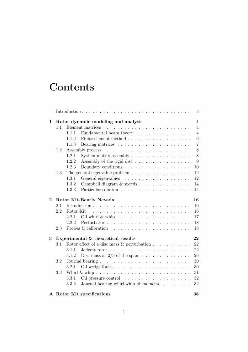
Contents

Introduction . . . . . . . . . . . . . . . . . . . . . . . . . . . . . . . 3

1 Rotor dynamic modeling and analysis 41.1 Element matrices . . . . . . . . . . . . . . . . . . . . . . . . . 4

1.1.1 Fundamental beam theory . . . . . . . . . . . . . . . . 41.1.2 Finite element method . . . . . . . . . . . . . . . . . . 61.1.3 Bearing matrices . . . . . . . . . . . . . . . . . . . . . 7

1.2 Assembly process . . . . . . . . . . . . . . . . . . . . . . . . . 81.2.1 System matrix assembly . . . . . . . . . . . . . . . . . 81.2.2 Assembly of the rigid disc . . . . . . . . . . . . . . . . 91.2.3 Boundary conditions . . . . . . . . . . . . . . . . . . . 10

1.3 The general eigenvalue problem . . . . . . . . . . . . . . . . . 121.3.1 General eigenvalues . . . . . . . . . . . . . . . . . . . 121.3.2 Campbell diagram & speeds . . . . . . . . . . . . . . . 141.3.3 Particular solution . . . . . . . . . . . . . . . . . . . . 14

2 Rotor Kit-Bently Nevada 162.1 Introduction . . . . . . . . . . . . . . . . . . . . . . . . . . . . 162.2 Rotor Kit . . . . . . . . . . . . . . . . . . . . . . . . . . . . . 16

2.2.1 Oil whirl & whip . . . . . . . . . . . . . . . . . . . . . 172.2.2 Perturbator . . . . . . . . . . . . . . . . . . . . . . . . 18

2.3 Probes & calibration . . . . . . . . . . . . . . . . . . . . . . . 18

3 Experimental & theoretical results 223.1 Rotor effect of a disc mass & perturbation . . . . . . . . . . . 22

3.1.1 Jeffcott rotor . . . . . . . . . . . . . . . . . . . . . . . 223.1.2 Disc mass at 2/3 of the span . . . . . . . . . . . . . . 26

3.2 Journal bearing . . . . . . . . . . . . . . . . . . . . . . . . . . 303.2.1 Oil wedge force . . . . . . . . . . . . . . . . . . . . . . 30

3.3 Whirl & whip . . . . . . . . . . . . . . . . . . . . . . . . . . . 313.3.1 Oil pressure control . . . . . . . . . . . . . . . . . . . 323.3.2 Journal bearing whirl-whip phenomena . . . . . . . . 32

A Rotor Kit specifications 38

1

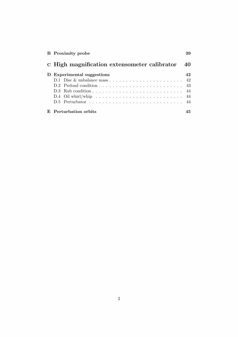
B Proximity probe 39

C High magnification extensometer calibrator 40

D Experimental suggestions 42D.1 Disc & unbalance mass . . . . . . . . . . . . . . . . . . . . . . 42D.2 Preload condition . . . . . . . . . . . . . . . . . . . . . . . . . 43D.3 Rub condition . . . . . . . . . . . . . . . . . . . . . . . . . . . 44D.4 Oil whirl/whip . . . . . . . . . . . . . . . . . . . . . . . . . . 44D.5 Perturbator . . . . . . . . . . . . . . . . . . . . . . . . . . . . 44

E Perturbation orbits 45

2

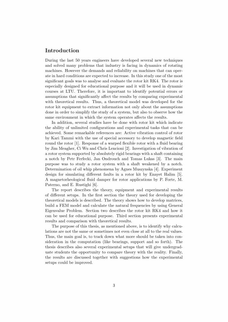
Introduction

During the last 50 years engineers have developed several new techniquesand solved many problems that industry is facing in dynamics of rotatingmachines. However the demands and reliability on machines that can oper-ate in hard conditions are expected to increase. In this study one of the mostsignificant goals was to analyse and evaluate the rotor kit RK4. The rotor isespecially designed for educational purpose and it will be used in dynamiccourses at LTU. Therefore, it is important to identify potential errors orassumptions that significantly affect the results by comparing experimentalwith theoretical results. Thus, a theoretical model was developed for therotor kit equipment to extract information not only about the assumptionsdone in order to simplify the study of a system, but also to observe how thesame environment in which the system operates affects the results.

In addition, several studies have be done with rotor kit which indicatethe ability of unlimited configurations and experimental tasks that can beachieved. Some remarkable references are: Active vibration control of rotorby Kari Tammi with the use of special accessory to develop magnetic fieldround the rotor [1]. Response of a warped flexible rotor with a fluid bearingby Jim Meagher, Ci Wu and Chris Lencioni [2]. Investigation of vibration ofa rotor system supported by absolutely rigid bearings with a shaft containinga notch by Petr Ferfecki, Jan Ondrouch and Tomas Lukas [3]. The mainpurpose was to study a rotor system with a shaft weakened by a notch.Determination of oil whip phenomena by Agnes Muszynska [4]. Experimentdesign for simulating different faults in a rotor kit by Enayet Halim [5].A magnetorheological fluid damper for rotor applications by P. Forte, M.Paterno, and E. Rustighi [6].

The report describes the theory, equipment and experimental resultsof different setups. In the first section the theory used for developing thetheoretical models is described. The theory shows how to develop matrices,build a FEM model and calculate the natural frequencies by using GeneralEigenvalue Problem. Section two describes the rotor kit RK4 and how itcan be used for educational purpose. Third section presents experimentalresults and comparison with theoretical results.

The purpose of this thesis, as mentioned above, is to identify why calcu-lations are not the same or sometimes not even close at all to the real values.Thus, the main goal is, to track down what more should be taken into con-sideration in the computation (like bearings, support and so forth). Thethesis describes also several experimental setups that will give undergrad-uate students the opportunity to compare theory with the reality. Finally,the results are discussed together with suggestions how the experimentalsetups could be improved.

3

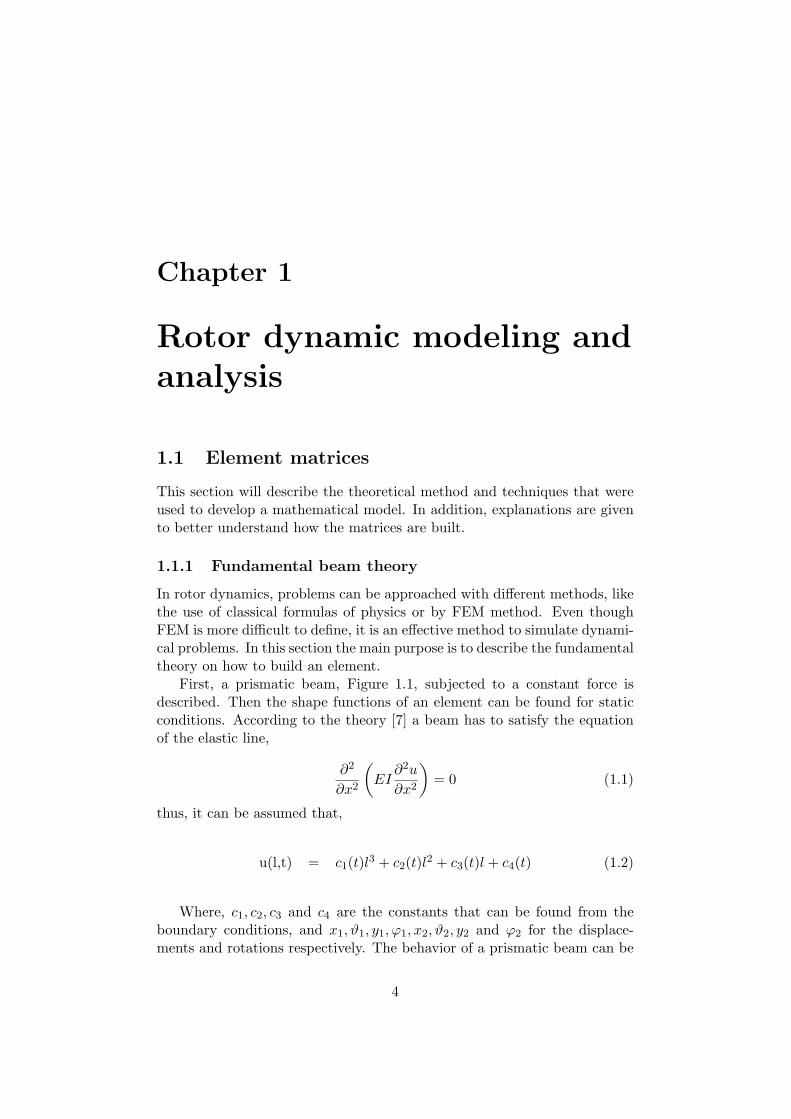
Chapter 1

Rotor dynamic modeling andanalysis

1.1 Element matrices

This section will describe the theoretical method and techniques that wereused to develop a mathematical model. In addition, explanations are givento better understand how the matrices are built.

1.1.1 Fundamental beam theory

In rotor dynamics, problems can be approached with different methods, likethe use of classical formulas of physics or by FEM method. Even thoughFEM is more difficult to define, it is an effective method to simulate dynami-cal problems. In this section the main purpose is to describe the fundamentaltheory on how to build an element.

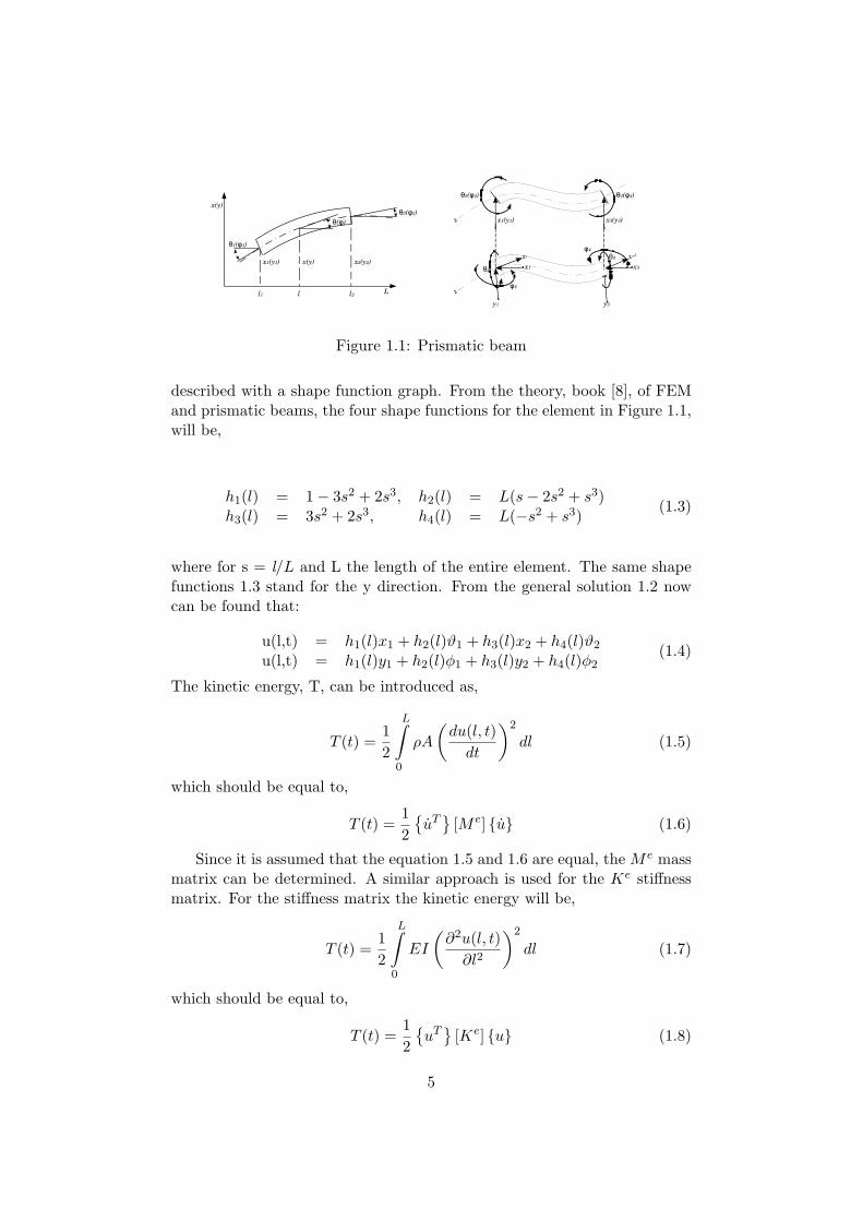
First, a prismatic beam, Figure 1.1, subjected to a constant force isdescribed. Then the shape functions of an element can be found for staticconditions. According to the theory [7] a beam has to satisfy the equationof the elastic line,

∂2

∂x2

(EI

∂2u

∂x2

)= 0 (1.1)

thus, it can be assumed that,

u(l,t) = c1(t)l3 + c2(t)l2 + c3(t)l + c4(t) (1.2)

Where, c1, c2, c3 and c4 are the constants that can be found from theboundary conditions, and x1, ϑ1, y1, ϕ1, x2, ϑ2, y2 and ϕ2 for the displace-ments and rotations respectively. The behavior of a prismatic beam can be

4

l1 l l2 L

x(y)

θ1(φ1)

( )θ φθ2(φ2)

x1(y1) x(y) x2(y2)

x3(y3)x1(y1)

θ2(φ2) θ4(φ4)

z

z

x1

y1

θ2

φ2

zi zi+1

y3

φ4

θ4

x3

Figure 1.1: Prismatic beam

described with a shape function graph. From the theory, book [8], of FEMand prismatic beams, the four shape functions for the element in Figure 1.1,will be,

h1(l) = 1− 3s2 + 2s3, h2(l) = L(s− 2s2 + s3)h3(l) = 3s2 + 2s3, h4(l) = L(−s2 + s3)

(1.3)

where for s = l/L and L the length of the entire element. The same shapefunctions 1.3 stand for the y direction. From the general solution 1.2 nowcan be found that:

u(l,t) = h1(l)x1 + h2(l)ϑ1 + h3(l)x2 + h4(l)ϑ2

u(l,t) = h1(l)y1 + h2(l)φ1 + h3(l)y2 + h4(l)φ2(1.4)

The kinetic energy, T, can be introduced as,

T (t) =12

L∫0

ρA

(du(l, t)dt

)2

dl (1.5)

which should be equal to,

T (t) =12{uT}

[M e] {u} (1.6)

Since it is assumed that the equation 1.5 and 1.6 are equal, the M e massmatrix can be determined. A similar approach is used for the Ke stiffnessmatrix. For the stiffness matrix the kinetic energy will be,

T (t) =12

L∫0

EI

(∂2u(l, t)∂l2

)2

dl (1.7)

which should be equal to,

T (t) =12{uT}

[Ke] {u} (1.8)

5

After the integration the elements of matrix Ke can be identified. Everypart that can be described with matrices, from now on can be called a finiteelement. The inverse of the stiffness matrix A(e) = K(e)−1 is the flexibilitymatrix [9] .

1.1.2 Finite element method

Finite element is today a frequently used method which help engineers tocreate models. The accuracy of the results is related on how many elementsare used for a problem. However, that does not imply that one has to useas many elements as possible. For instance, if it is of interest to find the1st and 2nd natural frequency of a beam problem it is enough to use onlytwo-four elements.

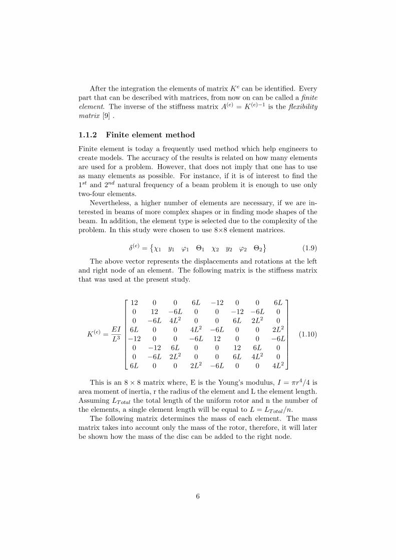
Nevertheless, a higher number of elements are necessary, if we are in-terested in beams of more complex shapes or in finding mode shapes of thebeam. In addition, the element type is selected due to the complexity of theproblem. In this study were chosen to use 8×8 element matrices.

δ(e) ={χ1 y1 ϕ1 Θ1 χ2 y2 ϕ2 Θ2

}(1.9)

The above vector represents the displacements and rotations at the leftand right node of an element. The following matrix is the stiffness matrixthat was used at the present study.

K(e) =EI

L3

12 0 0 6L −12 0 0 6L0 12 −6L 0 0 −12 −6L 00 −6L 4L2 0 0 6L 2L2 0

6L 0 0 4L2 −6L 0 0 2L2

−12 0 0 −6L 12 0 0 −6L0 −12 6L 0 0 12 6L 00 −6L 2L2 0 0 6L 4L2 0

6L 0 0 2L2 −6L 0 0 4L2

(1.10)

This is an 8 × 8 matrix where, E is the Young’s modulus, I = πr4/4 isarea moment of inertia, r the radius of the element and L the element length.Assuming LTotal the total length of the uniform rotor and n the number ofthe elements, a single element length will be equal to L = LTotal/n.

The following matrix determines the mass of each element. The massmatrix takes into account only the mass of the rotor, therefore, it will laterbe shown how the mass of the disc can be added to the right node.

6

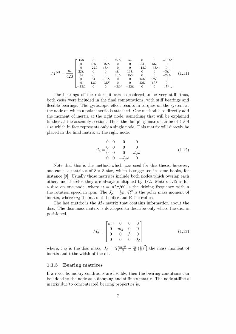
M (e) =m

420

156 0 0 22L 54 0 0 −13L0 156 −22L 0 0 54 13L 00 −22L 4L2 0 0 −13L −3L2 0

22L 0 0 4L2 13L 0 0 −3L2

54 0 0 13L 156 0 0 −22L0 54 −13L 0 0 156 22L 00 13L −3L2 0 0 22L 4L2 0−13L 0 0 −3L2 −22L 0 0 4L2

(1.11)

The bearings of the rotor kit were considered to be very stiff, thus,both cases were included in the final computations, with stiff bearings andflecible bearings. The gyroscopic effect results in torques on the system atthe node on which a polar inertia is attached. One method is to directly addthe moment of inertia at the right node, something that will be explainedfurther at the assembly section. Thus, the damping matrix can be of 4× 4size which in fact represents only a single node. This matrix will directly beplaced in the final matrix at the right node.

Cd =

0 0 0 00 0 0 00 0 0 Jpω0 0 −Jpω 0

(1.12)

Note that this is the method which was used for this thesis, however,one can use matrices of 8 × 8 size, which is suggested in some books, forinstance [9]. Usually those matrices include both nodes which overlap eachother, and therefor they are always multiplied by 1/2. Matrix 1.12 is fora disc on one node, where ω = n2π/60 is the driving frequency with nthe rotation speed in rpm. The Jp = 1

2mdR2 is the polar mass moment of

inertia, where md the mass of the disc and R the radius.The last matrix is the Md matrix that contains information about the

disc. The disc mass matrix is developed to describe only where the disc ispositioned,

Md =

md 0 0 00 md 0 00 0 Jd 00 0 0 Jd

(1.13)

where, md is the disc mass, Jd = 2[mR2

8 + m6

(t2

)2] the mass moment ofinertia and t the width of the disc.

1.1.3 Bearing matrices

If a rotor boundary conditions are flecible, then the bearing conditions canbe added to the node as a damping and stiffness matrix. The node stiffnessmatrix due to concentrated bearing properties is,

7

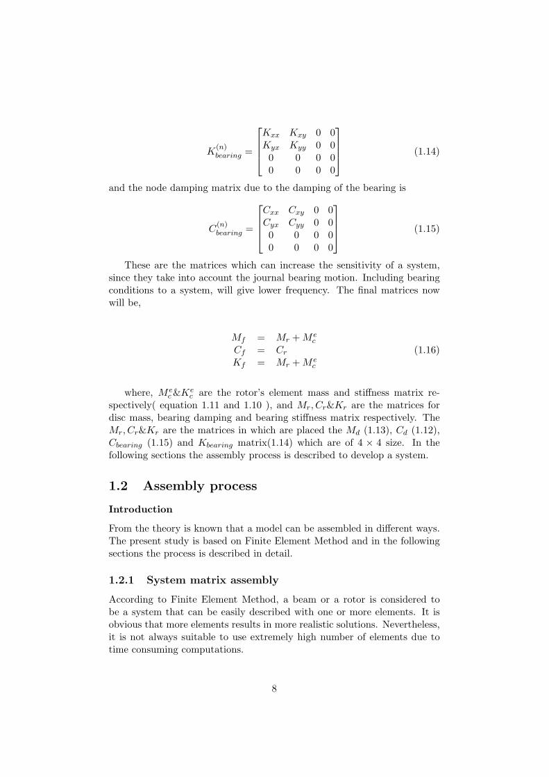
K(n)bearing =

Kxx Kxy 0 0Kyx Kyy 0 0

0 0 0 00 0 0 0

(1.14)

and the node damping matrix due to the damping of the bearing is

C(n)bearing =

Cxx Cxy 0 0Cyx Cyy 0 00 0 0 00 0 0 0

(1.15)

These are the matrices which can increase the sensitivity of a system,since they take into account the journal bearing motion. Including bearingconditions to a system, will give lower frequency. The final matrices nowwill be,

Mf = Mr +M ec

Cf = CrKf = Mr +M e

c

(1.16)

where, M ec&Ke

c are the rotor’s element mass and stiffness matrix re-spectively( equation 1.11 and 1.10 ), and Mr, Cr&Kr are the matrices fordisc mass, bearing damping and bearing stiffness matrix respectively. TheMr, Cr&Kr are the matrices in which are placed the Md (1.13), Cd (1.12),Cbearing (1.15) and Kbearing matrix(1.14) which are of 4 × 4 size. In thefollowing sections the assembly process is described to develop a system.

1.2 Assembly process

Introduction

From the theory is known that a model can be assembled in different ways.The present study is based on Finite Element Method and in the followingsections the process is described in detail.

1.2.1 System matrix assembly

According to Finite Element Method, a beam or a rotor is considered tobe a system that can be easily described with one or more elements. It isobvious that more elements results in more realistic solutions. Nevertheless,it is not always suitable to use extremely high number of elements due totime consuming computations.

8

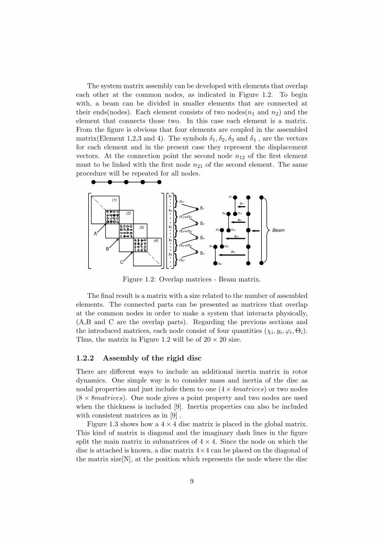
The system matrix assembly can be developed with elements that overlapeach other at the common nodes, as indicated in Figure 1.2. To beginwith, a beam can be divided in smaller elements that are connected attheir ends(nodes). Each element consists of two nodes(n1 and n2) and theelement that connects those two. In this case each element is a matrix.From the figure is obvious that four elements are coupled in the assembledmatrix(Element 1,2,3 and 4). The symbols δ1, δ2, δ3 and δ4 , are the vectorsfor each element and in the present case they represent the displacementvectors. At the connection point the second node n12 of the first elementmust to be linked with the first node n21 of the second element. The sameprocedure will be repeated for all nodes.

(1)

(2)

(3)

(4)

A

B

C

δ1

x1

x2

x5

x4

x3

}}}}}n42

n11

n12+n21

n22+n31

n32+n41

δ2

δ3

δ4

Beam

n11

n42

n12n21

n22n31

n32n41

e(3)

e(4)

e(1)

e(2)

Figure 1.2: Overlap matrices - Beam matrix.

The final result is a matrix with a size related to the number of assembledelements. The connected parts can be presented as matrices that overlapat the common nodes in order to make a system that interacts physically,(A,B and C are the overlap parts). Regarding the previous sections andthe introduced matrices, each node consist of four quantities (χi, yi, ϕi,Θi).Thus, the matrix in Figure 1.2 will be of 20× 20 size.

1.2.2 Assembly of the rigid disc

There are different ways to include an additional inertia matrix in rotordynamics. One simple way is to consider mass and inertia of the disc asnodal properties and just include them to one (4× 4matrices) or two nodes(8 × 8matrices). One node gives a point property and two nodes are usedwhen the thickness is included [9]. Inertia properties can also be includedwith consistent matrices as in [9] .

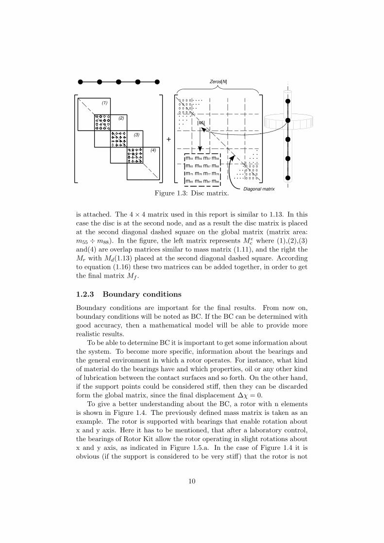
Figure 1.3 shows how a 4× 4 disc matrix is placed in the global matrix.This kind of matrix is diagonal and the imaginary dash lines in the figuresplit the main matrix in submatrices of 4× 4. Since the node on which thedisc is attached is known, a disc matrix 4×4 can be placed on the diagonal ofthe matrix size[N], at the position which represents the node where the disc

9

(1)

(2)

(3)

(4)

+

0 0 0 0 • • • •0 0 0 0 • • •0 0 0 0 • • 0 0 0 0 •• • • •• • •• • •

• • • • • • • • • • • 0 0 0 0 • • 0 0 0 0 • • • 0 0 0 0 • • • • 0 0 0 0

[Md]

Zeros[N]

m55 m56 m57 m58

m85

m65

m75

m86

m66

m76

m87

m67

m77

m88

m68

m78

Diagonal matrixFigure 1.3: Disc matrix.

is attached. The 4× 4 matrix used in this report is similar to 1.13. In thiscase the disc is at the second node, and as a result the disc matrix is placedat the second diagonal dashed square on the global matrix (matrix area:m55 ÷m88). In the figure, the left matrix represents M e

c where (1),(2),(3)and(4) are overlap matrices similar to mass matrix (1.11), and the right theMr with Md(1.13) placed at the second diagonal dashed square. Accordingto equation (1.16) these two matrices can be added together, in order to getthe final matrix Mf .

1.2.3 Boundary conditions

Boundary conditions are important for the final results. From now on,boundary conditions will be noted as BC. If the BC can be determined withgood accuracy, then a mathematical model will be able to provide morerealistic results.

To be able to determine BC it is important to get some information aboutthe system. To become more specific, information about the bearings andthe general environment in which a rotor operates. For instance, what kindof material do the bearings have and which properties, oil or any other kindof lubrication between the contact surfaces and so forth. On the other hand,if the support points could be considered stiff, then they can be discardedform the global matrix, since the final displacement ∆χ = 0.

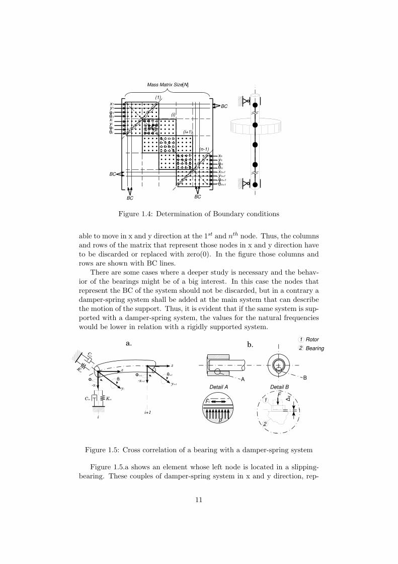
To give a better understanding about the BC, a rotor with n elementsis shown in Figure 1.4. The previously defined mass matrix is taken as anexample. The rotor is supported with bearings that enable rotation aboutx and y axis. Here it has to be mentioned, that after a laboratory control,the bearings of Rotor Kit allow the rotor operating in slight rotations aboutx and y axis, as indicated in Figure 1.5.a. In the case of Figure 1.4 it isobvious (if the support is considered to be very stiff) that the rotor is not

10

(1)

(i)

(i+1)

(n1)

[Md]

Mass Matrix Size[N]

• • • •• • • •• • • •

• • • •

• • • •• • • •• • • •

• • • •

• • • •• • • •• • • •

• • • •

• • • •• • • •• • • •

• • • •

• • • •• • • •• • • •

• • • •• • • •• • • •• • • •

• • • •

• • • •• • • •• • • •

• • • •

• • • •• • • •• • • •

• • • •

• • • •• • • •• • • •

• • • •

• • • •• • • •• • • •

• • • •

xnynφnθnxn+1yn+1φn+1

θn+1

x1y1

φ1θ1xiyiφi

θi

BCBC

BC

BC

Figure 1.4: Determination of Boundary conditions

able to move in x and y direction at the 1st and nth node. Thus, the columnsand rows of the matrix that represent those nodes in x and y direction haveto be discarded or replaced with zero(0). In the figure those columns androws are shown with BC lines.

There are some cases where a deeper study is necessary and the behav-ior of the bearings might be of a big interest. In this case the nodes thatrepresent the BC of the system should not be discarded, but in a contrary adamper-spring system shall be added at the main system that can describethe motion of the support. Thus, it is evident that if the same system is sup-ported with a damper-spring system, the values for the natural frequencieswould be lower in relation with a rigidly supported system.

ΔχKxx

xi

xi+1yi+1

yi

zz

θiΦi

θi+1Φi+1

Cxx

Cyy

Kyy

ii+1

A B

Detail A Detail BF

1

2

1

2

Rotor

Bearing

p

Ff

a. b.

Figure 1.5: Cross correlation of a bearing with a damper-spring system

Figure 1.5.a shows an element whose left node is located in a slipping-bearing. These couples of damper-spring system in x and y direction, rep-

11

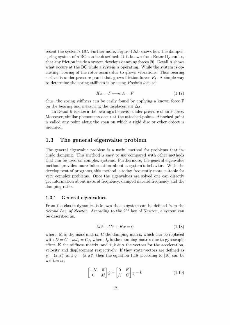
resent the system’s BC. Further more, Figure 1.5.b shows how the damper-spring system of a BC can be described. It is known from Rotor Dynamics,that any friction inside a system develops damping forces [9]. Detail A showswhat occurs at the BC while a system is operating. While the system is op-erating, bowing of the rotor occurs due to grown vibrations. Thus bearingsurface is under pressure p and that grows friction forces Ff . A simple wayto determine the spring stiffness is by using Hooke’s law, as:

Kx = F←→σA = F (1.17)

thus, the spring stiffness can be easily found by applying a known force Fon the bearing and measuring the displacement ∆x.

In Detail B is shown the bearing’s behavior under pressure of an F force.Moreover, similar phenomena occur at the attached points. Attached pointis called any point along the span on which a rigid disc or other object ismounted.

1.3 The general eigenvalue problem

The general eigenvalue problem is a useful method for problems that in-clude damping. This method is easy to use compared with other methodsthat can be used on complex systems. Furthermore, the general eigenvaluemethod provides more information about a system’s behavior. With thedevelopment of programs, this method is today frequently more suitable forvery complex problems. Once the eigenvalues are solved one can directlyget information about natural frequency, damped natural frequency and thedamping ratio.

1.3.1 General eigenvalues

From the classic dynamics is known that a system can be defined from theSecond Law of Newton. According to the 2nd law of Newton, a system canbe described as,

Mx+ Cx+Kx = 0 (1.18)

where, M is the mass matrix, C the damping matrix which can be replacedwith D = C +ωJp = Cf , where Jp is the damping matrix due to gyroscopiceffect, K the stiffness matrix, and x, x & x the vectors for the acceleration,velocity and displacement respectively. If they state vectors are defined asy = (x x)′ and y = (x x)′, then the equation 1.18 according to [10] can bewritten as, [

−K 00 M

]y +

[0 KK C

]y = 0 (1.19)

12

or [−I 00 M

]y +

[0 IK C

]y = 0

where, I is the unit diagonal matrix and 0 zero matrix. Assuming that thefirst matrix is -S and the second R, the equation 1.19 becomes,

−Sy +Ry = 0 (1.20)

Assuming a solution as y = CY eλt, then the problem becomes an eigenvalueproblem, and the equation 1.20 can be turned into,

[R− λS]Y = 0,

[A− λI]Y = 0, (1.21)

or [R−1S − 1

λI

]Y = 0

The eigenvalues λ can now be determined from the equations 1.21, sinceit is known that A = S−1R. With the use of a mathematical program, theeigenvalues can be extracted directly from A. In rotordynamics the mostinteresting is to plot the imaginary part of the eigenvalues to get the Camp-bell diagram, see Figure 1.6. Since, the eigenvalues are known the Y can beeasily determined.

yh(t) =n∑i=1

CiYieλit (1.22)

The Ci can be solved for known initial conditions with a mathematicalprogram. If E is the matrix with the eigenvectors,

E = [Y1, Y2, ..., Yn] (1.23)

then the constants can be determined from the following equation:

C = E−1yh(0) (1.24)

Having the solved constants from 1.24, in equation 1.23 the motion of aunforced system can be analysed.

13

•

••

= ω Ω

= ω Ω

ωn

ωn

ωn+1

ωn+2

ωn+3

ωn+5

ωn+4

ωn+6

••

• ••

•

W1 W2

W1 W2

W3

Backward

Forward

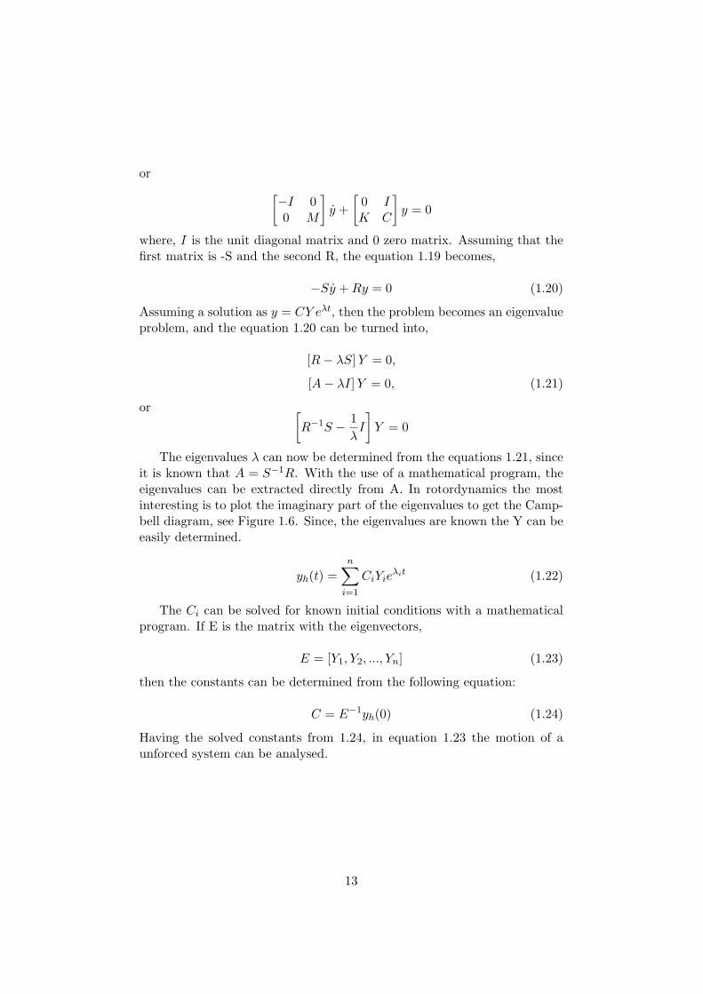
Figure 1.6: Campbell Diagram

1.3.2 Campbell diagram & speeds

Since the main topic deals with rotor dynamics, it is important to mentionabout the Campbell diagram. As shown in Figure 1.6, once the eigenvaluesare solved, then the imaginary part can be plotted in order to see how thegyroscopic effect acts on the rotor. Moreover, Campbell diagram shows theresonances of a system, either these are operating forward or backward.

To begin with, Campbell diagram includes, two straight lines ω whichare the driving frequencies for forward and backward direction, and sev-eral lines ωn+1, ...., ωn+6 whose intersection with the driving frequency(dashlines) shows the resonance. The curves ωn+1, ωn+2 & ωn+3 are positive whichindicates that the whirl has the same direction as the angular velocity of therotor, and is called Forward precession [9]. The curves ωn+4, ωn+5 & ωn+6

are negative, which indicates that the whirl has opposite direction relatedto the rotor’s, and is called Backward precession [9]. At the right of thesame figure are the mode shapes (Wi) of the shaft for backward and forwardfrequency.

In Figure 1.6, is the Campbell diagram of a Jeffcott rotor. The disc isplaced at the midspan of the shaft and as it can be seen from the diagramthere is no gyroscopic effect at the first resonance speed. The eigenfrequen-cies ωn+3 and ωn+4 are just straight lines with the same value for forwardand backward precession.

1.3.3 Particular solution

The general eigenvalue problem gives solution for systems without externalforce. This force can be a small unbalanced mass that develops centrifugalforces. Those centrifugal forces increase the systems amplitude, especiallywhen a rotor operates close to resonances. Note that, if one is aiming to

14

exceed the critical speed(which in fact is the most crucial), the rotor shouldaccelerate fast through this critical area. According to [10] for particularsolution the 2nd law of Newton becomes,

Mx+Dx+Kx = fs sin(ωt) + fc cos(ωt) (1.25)

where, the two vectors fs and fc are forces. According to the theory [10], aharmonic input on a linear system can only result in a harmonic output ofequal frequency, and therefore it can be assumed that,

x = a sin(ωt) + b cos(ωt) = as+ bc (1.26)

where, a and b are real vectors. Thus, the equation of motion becomes,

[K − ω2M ][as+ bc] + ωD[ac− bs] = fss+ fcc (1.27)

By separating the equation 1.27 in s and c term, it becomes two equa-tions, [

K − ω2M]a− ωDb = fs[

K − ω2M]b− ωDa = fc

(1.28)

To simplify the equations 1.28, it is assumed that K = [K − ω2M ], so theequation bocomes, [

K]a− ωDb = fs[

K]b− ωDa = fc

(1.29)

Solving the equations 1.29 by the terms a and b, the problem is solved.

b =[K + ω2DK−1D

]−1 [fc − ωDKfs

]a = K−1fs + ωK−1Db

(1.30)

Note that the ω is the driving frequency of the system. In addition, thisa method that assumes that the system includes damping that is not equalto zeros, D 6= 0. The amplitude can be found from the resultant of a and b,and if R is the amplitude then,

R =√a2 + b2 (1.31)

If the R is plotted, then the resonance frequencies can be found for actualforcing.

15

Chapter 2

Rotor Kit-Bently Nevada

2.1 Introduction

Bently Nevada Rotor Kit RK-4, is a rotating machine that can be adapted indifferent configurations and is suitable for educational purposes. The RotorKit comes along with different accessories that can provide different optionsand a wide number of experimental tasks.

• Rotor speed• Shaft bow• Rotor stiffness• Amount and angle of unbalance• Shaft rub or hitting condition• Rotor-bearing relationships

The user is able to perform many different experiments and compare thefinal results with a theoretical model. The advantage of this experimentalequipment, is that one can verify that theoretical calculations give realisticvalues, or values that are close to the real ones. Moreover, this is one wayto verify that assumptions in a theoretical model are valid.

2.2 Rotor Kit

The rotor kit is shown in Figure 2.1. In the mounting blocks probes areused to measure the displacement of the rotor at different positions of theshaft. All the outputs will be displayed by a simple program in LabView oran oscillator. It is important that the rotor is set up on a rigid base to avoiddisturbances that can influence the measurements.

Figure 2.1 shows one of the numerous setups that can be achieved withthis equipment. Two disc are available that can be placed in any position onthe rotor. Further more, constant forces and unbalanced masses can easily

16

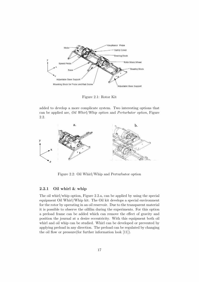
Figure 2.1: Rotor Kit

added to develop a more complicate system. Two interesting options thatcan be applied are, Oil Whirl/Whip option and Perturbator option, Figure2.2.

a. b.

z

x

y

Figure 2.2: Oil Whirl/Whip and Perturbator option

2.2.1 Oil whirl & whip

The oil whirl/whip option, Figure 2.2.a, can be applied by using the specialequipment Oil Whirl/Whip kit. The Oil kit develops a special environmentfor the rotor by operating in an oil reservoir. Due to the transparent materialit is possible to observe the oilfilm during the experiments. For this optiona preload frame can be added which can remove the effect of gravity andposition the journal at a desire eccentricity. With this equipment both oilwhirl and oil whip can be studied. Whirl can be developed or prevented byapplying preload in any direction. The preload can be regulated by changingthe oil flow or pressure(for further information look [11]).

17

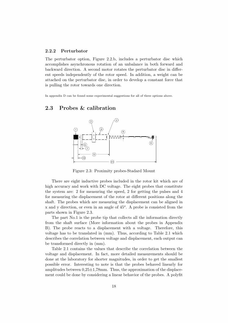
2.2.2 Perturbator

The perturbator option, Figure 2.2.b, includes a perturbator disc whichaccomplishes asynchronous rotation of an unbalance in both forward andbackward direction. A second motor rotates the perturbator disc in differ-ent speeds independently of the rotor speed. In addition, a weight can beattached on the perturbator disc, in order to develop a constant force thatis pulling the rotor towards one direction.

In appendix D can be found some experimental suggestions for all of three options above.

2.3 Probes & calibration

Figure 2.3: Proximity probes-Stadard Mount

There are eight inductive probes included in the rotor kit which are ofhigh accuracy and work with DC voltage. The eight probes that constitutethe system are: 2 for measuring the speed, 2 for getting the pulses and 4for measuring the displacement of the rotor at different positions along theshaft. The probes which are measuring the displacement can be aligned inx and y direction, or even in an angle of 45o. A probe is consisted from theparts shown in Figure 2.3.

The part No.1 is the probe tip that collects all the information directlyfrom the shaft surface (More information about the probes in AppendixB). The probe reacts to a displacement with a voltage. Therefore, thisvoltage has to be translated in (mm). Thus, according to Table 2.1 whichdescribes the correlation between voltage and displacement, each output canbe transformed directly in (mm).

Table 2.1 contains the values that describe the correlation between thevoltage and displacement. In fact, more detailed measurements should bedone at the laboratory for shorter magnitudes, in order to get the smallestpossible error. Interesting to note is that the probes behaved linearly foramplitudes between 0,25±1,78mm. Thus, the approximation of the displace-ment could be done by considering a linear behavior of the probes. A polyfit

18

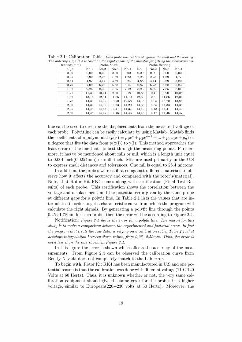
Table 2.1: Calibration Table. Each probe was calibrated against the shaft and the bearing.The ordering 1,2,3 & 4 is based on the input canals of the monitor for getting the measurements.

Distance(mm) Probe-Shaft Probe-Bearinga \ a No.1 N0.2 No.3 No.4 No.1 No.2 No.3 No.40,00 0,00 0,00 0,00 0,00 0,00 0,00 0,00 0,000,25 2,90 2,25 1,69 1,22 2,96 2,25 1,69 1,770,51 4,97 4,14 3,69 3,24 4,88 4,14 3,69 3,800,76 7,09 6,23 5,68 5,14 6,87 6,23 5,68 5,831,02 9,26 8,39 7,85 7,19 8,93 8,39 7,85 8,011,27 11,30 10,41 9,90 9,18 10,83 10,41 9,90 10,081,52 13,14 12,31 11,86 11,10 12,60 12,31 11,86 12,041,78 14,30 14,05 13,70 12,58 14,18 14,05 13,70 13,862,00 14,39 14,35 14,33 14,20 14,35 14,35 14,33 14,342,25 14,45 14,43 14,41 14,37 14,42 14,43 14,41 14,422,50 14,48 14,47 14,46 14,43 14,46 14,47 14,46 14,47

line can be used to describe the displacements from the measured voltage ofeach probe. Polyfitline can be easily calculate by using Matlab. Matlab findsthe coefficients of a polynomial (p(x) = p1x

n + p2xn−1 + ...+ pn−1x+ pn) of

n degree that fits the data from p(x(i)) to y(i). This method approaches theleast error or the line that fits best through the measuring points. Further-more, it has to be mentioned about mils or mil, which is a length unit equalto 0.001 inch(0.0254mm) or milli-inch. Mils are used primarily in the U.Sto express small distances and tolerances. One mil is equal to 25.4 microns.

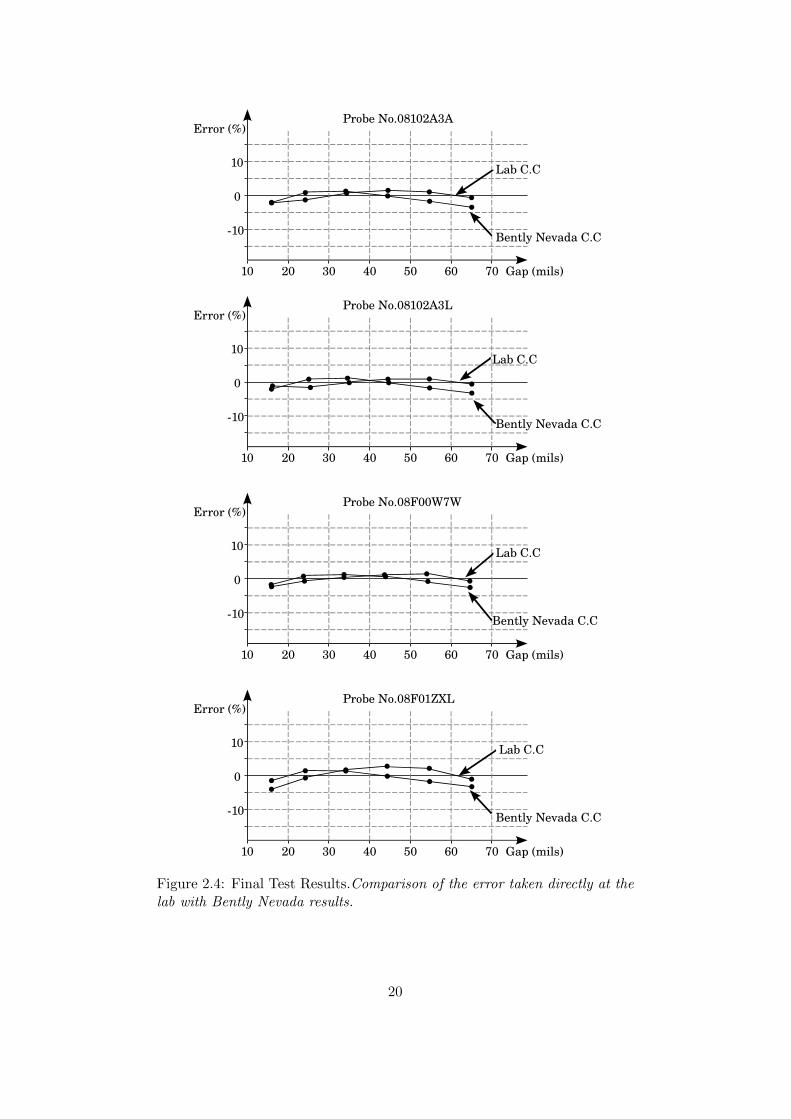
In addition, the probes were calibrated against different materials to ob-serve how it affects the accuracy and compared with the rotor’s(material).Note, that Rotor Kit RK4 comes along with certification (Final Test Re-sults) of each probe. This certification shows the correlation between thevoltage and displacement, and the potential error given by the same probeat different gaps for a polyfit line. In Table 2.1 lists the values that are in-terpolated in order to get a characteristic curve from which the program willcalculate the right signals. By generating a polyfit line through the points0,25÷1,78mm for each probe, then the error will be according to Figure 2.4.

Notification: Figure 2.4 shows the error for a polyfit line. The reason for thisstudy is to make a comparison between the experimental and factorial error. In factthe program that treats the raw data, is relying on a calibration table, Table 2.1, thatdevelops interpolation between those points, from 0,25÷2,50mm. Thus, the error iseven less than the one shown in Figure 2.4.

In this figure the error is shown which affects the accuracy of the mea-surements. From Figure 2.4 can be observed the calibration curve fromBently Nevada does not completely match to the Lab error.

To begin with, Rotor Kit RK4 has been manufactured in U.S and one po-tential reason is that the calibration was done with different voltage(110÷120Volts at 60 Hertz). Thus, it is unknown whether or not, the very same cal-ibration equipment should give the same error for the probes in a highervoltage, similar to European(220÷230 volts at 50 Hertz). Moreover, the

19

0

10

10

10 20 30 40 50 60 70 Gap (mils)

Error (%)Probe No.08102A3A

Bently Nevada C.C

Lab C.C

0

10

10

10 20 30 40 50 60 70 Gap (mils)

Error (%)Probe No.08102A3L

Bently Nevada C.C

Lab C.C

0

10

10

10 20 30 40 50 60 70 Gap (mils)

Error (%)Probe No.08F00W7W

Bently Nevada C.C

Lab C.C

0

10

10

10 20 30 40 50 60 70 Gap (mils)

Error (%)Probe No.08F01ZXL

Bently Nevada C.C

Lab C.C

Figure 2.4: Final Test Results.Comparison of the error taken directly at thelab with Bently Nevada results.

20

calibration process was accomplished with different equipment than the oneused by Bently Nevada. The calibrator used for this purpose is described inAppendix C. At the lab was marked that the probes gave a characteristicline that was parallel to Bently Nevada’s, but slightly higher along the volt-age axis. One additional reason can be the environmental temperature andthe wiring from the output to voltmeter. Finally, one reason can be thatthe calibration was done against another material.

21

Chapter 3

Experimental & theoreticalresults

The present chapter compares experimental and theoretical results. Thepurpose is to scale down the problem before will be adapted in real di-mensions. The experiments which will be explained in this section, wereaccomplished with Rotor Kit RK4 Bently Nevada. Furthermore, dis-cussion will take place for each experiment to evaluate theoretical modelswhich were developed in order to describe the same experimental systems.

3.1 Rotor effect of a disc mass & perturbation

This task shows how a system responses, while a perturbator attached on theshaft rolling back or forth. In fact, perturbator is an independent part of thesystem, whose main purpose is the determination of the system’s dynamicstiffness [12] related only to the rotational velocity. In this case a systemhas constant speed and the perturbator is running gradually. Furthermore,this is one method to identify potential lower modes of the system that weremuted while using synchronous perturbation for unknown reasons.

Last, according to [12] the given information of a nonsynchronous per-turbation, in comparison always with a synchronous perturbation, are morefruitful since, as it was mentioned above, a synchronous perturbation is af-fected by the very same system as a result of information that can not beobservable.

3.1.1 Jeffcott rotor

This subsection describes the experimental result of a Jeffcott Rotor andcompares with the theoretical model of the same system. Note that, Jeffcottrotor is called every system with the disc mass placed at the midspan of therotating shaft. To begin with, the demonstration was executed with a disc

22

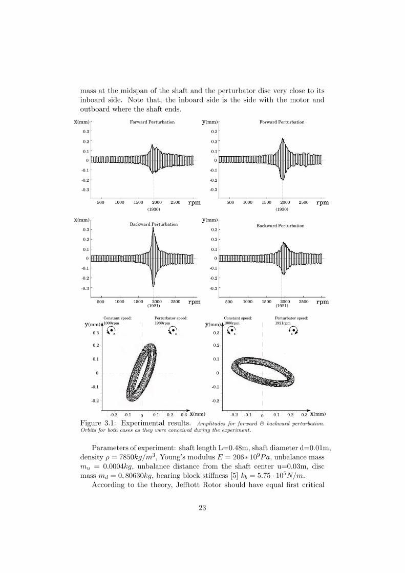
mass at the midspan of the shaft and the perturbator disc very close to itsinboard side. Note that, the inboard side is the side with the motor andoutboard where the shaft ends.

0

0.1

0.2

0.3

0.3

0.2

0.1

0

0.1

0.2

0.3

0.3

0.2

0.1

rpm

x(mm)

rpm

y(mm)

500 1000 1500 2000 2500 500 1000 1500 2000 2500

(1930) (1930)

0

0

0.1

0.2

0.3

0.1

0.2

0.2 0.1 0.1 0.2 0.3

•z •z

Constant speed:1000rpm

Perturbator speed:1930rpmy(mm)

x(mm)

Forward Perturbation Forward Perturbation

0

0

0.1

0.2

0.3

0.1

0.2

0.2 0.1 0.1 0.2 0.3

•z •z



x(mm)

(1921)(1921)

Backward Perturbation Backward Perturbation

rpm500 1000 1500 2000 2500 rpm500 1000 1500 2000 2500

0

0.1

0.2

0.3

0.3

0.2

0.1

x(mm)

0

0.1

0.2

0.3

0.3

0.2

0.1

y(mm)

Figure 3.1: Experimental results. Amplitudes for forward & backward perturbation.Orbits for both cases as they were conceived during the experiment.

Parameters of experiment: shaft length L=0.48m, shaft diameter d=0.01m,density ρ = 7850kg/m3, Young’s modulus E = 206∗109Pa, unbalance massmu = 0.0004kg, unbalance distance from the shaft center u=0.03m, discmass md = 0, 80630kg, bearing block stiffness [5] kb = 5.75 · 105N/m.

According to the theory, Jefftott Rotor should have equal first critical

23

speed for forward and backward rotation. As it can be seen from Figure3.1, indeed the first critical speed matches for both cases with a very littledivergence, forward 1930rpm and backward 1921rpm. Thus, for both casesthe first critical speed is approximately ω ≈ 203rad/s. The first naturalfrequency is very obvious, due to the fact that suddenly a multiperiodicsolution becomes a large orbit of single frequency as shown in the figure.In this phase the orbits have the highest amplitude, and therefore, rotatingmachines should pass rapidly through this area because the consequencescan be severe.

These experiments as can be seen from the graphs, were executed forspeeds 200rpm-3000rpm. However, interesting was the behavior of the shaftwhen it was rapidly accelerated above 5000rpm for a very short period.The shaft behaves as almost a perfect balanced system in velocities abovethe first natural frequency, and the orbit gets smaller and smaller until thenext critical speed. Furthermore, even if the shaft changes amplitude, it iswhirling round the same axial line.

a. b.

c.ω(rad/s)

ω(rad/s) ω(rad/s)

ω(rad/s) ω(rad/s)

Perturbation guide

Simple model Simple model & Bearings

Entire model & Bearings

(215)(210.6)

(210.5)

ω(rad/s)

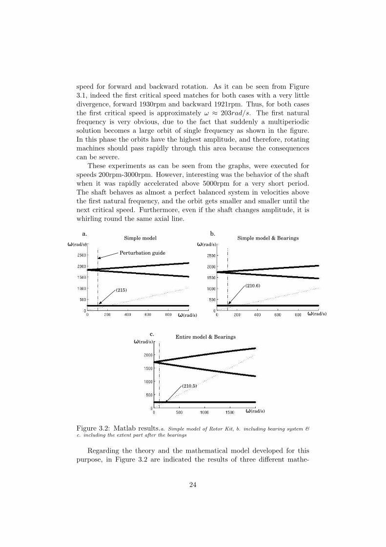
Figure 3.2: Matlab results.a. Simple model of Rotor Kit, b. including bearing system &c. including the extent part after the bearings

Regarding the theory and the mathematical model developed for thispurpose, in Figure 3.2 are indicated the results of three different mathe-

24

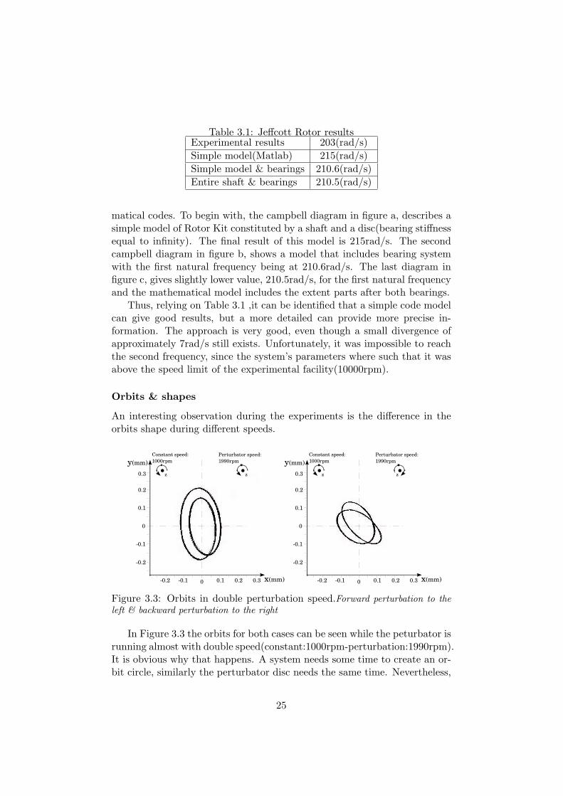
Table 3.1: Jeffcott Rotor resultsExperimental results 203(rad/s)Simple model(Matlab) 215(rad/s)Simple model & bearings 210.6(rad/s)Entire shaft & bearings 210.5(rad/s)

matical codes. To begin with, the campbell diagram in figure a, describes asimple model of Rotor Kit constituted by a shaft and a disc(bearing stiffnessequal to infinity). The final result of this model is 215rad/s. The secondcampbell diagram in figure b, shows a model that includes bearing systemwith the first natural frequency being at 210.6rad/s. The last diagram infigure c, gives slightly lower value, 210.5rad/s, for the first natural frequencyand the mathematical model includes the extent parts after both bearings.

Thus, relying on Table 3.1 ,it can be identified that a simple code modelcan give good results, but a more detailed can provide more precise in-formation. The approach is very good, even though a small divergence ofapproximately 7rad/s still exists. Unfortunately, it was impossible to reachthe second frequency, since the system’s parameters where such that it wasabove the speed limit of the experimental facility(10000rpm).

Orbits & shapes

An interesting observation during the experiments is the difference in theorbits shape during different speeds.

0

0

0.1

0.2

0.3

0.1

0.2

0.2 0.1 0.1 0.2 0.3

•z •z



x(mm) 0

0

0.1

0.2

0.3

0.1

0.2

0.2 0.1 0.1 0.2 0.3

•z •z



x(mm)

Figure 3.3: Orbits in double perturbation speed.Forward perturbation to theleft & backward perturbation to the right

In Figure 3.3 the orbits for both cases can be seen while the peturbator isrunning almost with double speed(constant:1000rpm-perturbation:1990rpm).It is obvious why that happens. A system needs some time to create an or-bit circle, similarly the perturbator disc needs the same time. Nevertheless,

25

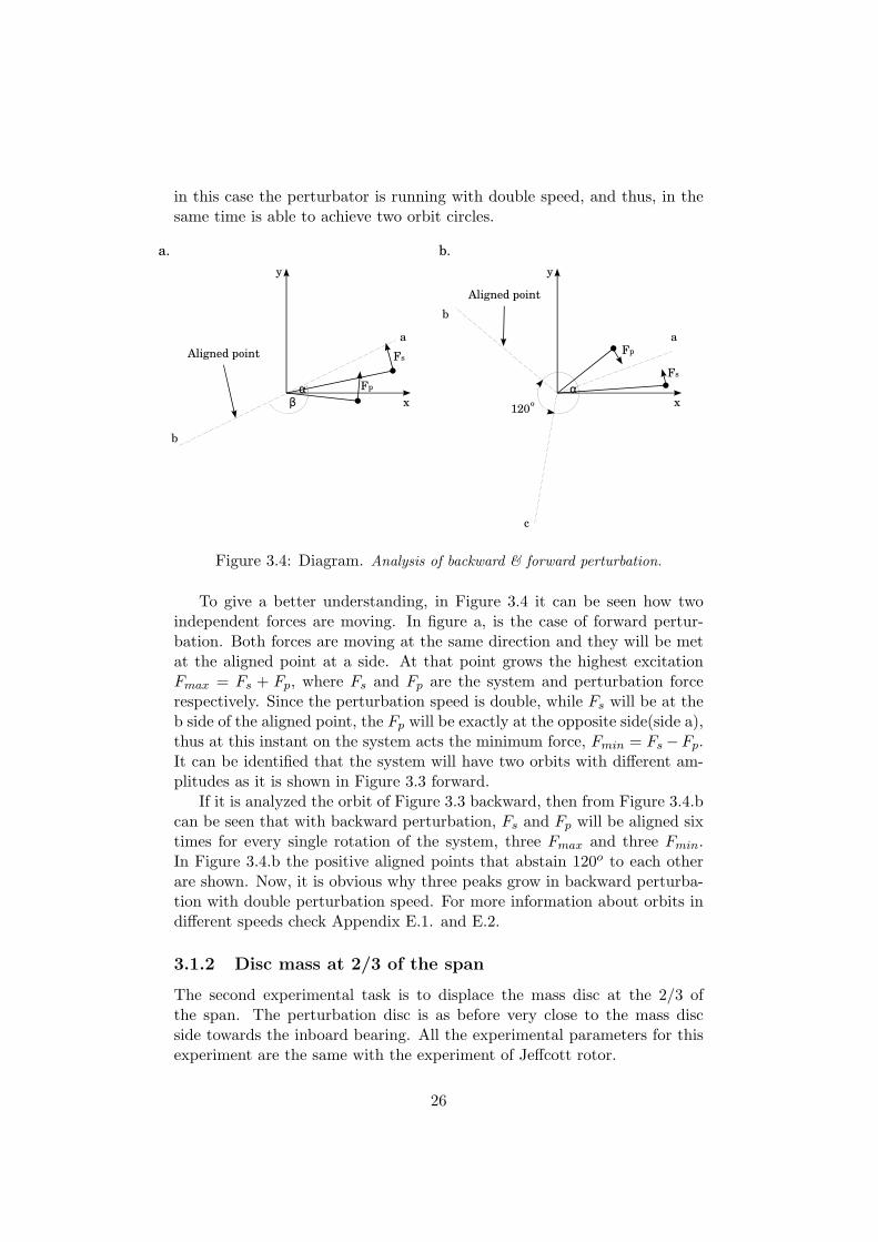
in this case the perturbator is running with double speed, and thus, in thesame time is able to achieve two orbit circles.

Aligned pointa

b

x

y

Fs

Fpαβ

Aligned point

a

b

x

y

Fs

Fp

α

c

120o

a. b.

Figure 3.4: Diagram. Analysis of backward & forward perturbation.

To give a better understanding, in Figure 3.4 it can be seen how twoindependent forces are moving. In figure a, is the case of forward pertur-bation. Both forces are moving at the same direction and they will be metat the aligned point at a side. At that point grows the highest excitationFmax = Fs + Fp, where Fs and Fp are the system and perturbation forcerespectively. Since the perturbation speed is double, while Fs will be at theb side of the aligned point, the Fp will be exactly at the opposite side(side a),thus at this instant on the system acts the minimum force, Fmin = Fs−Fp.It can be identified that the system will have two orbits with different am-plitudes as it is shown in Figure 3.3 forward.

If it is analyzed the orbit of Figure 3.3 backward, then from Figure 3.4.bcan be seen that with backward perturbation, Fs and Fp will be aligned sixtimes for every single rotation of the system, three Fmax and three Fmin.In Figure 3.4.b the positive aligned points that abstain 120o to each otherare shown. Now, it is obvious why three peaks grow in backward perturba-tion with double perturbation speed. For more information about orbits indifferent speeds check Appendix E.1. and E.2.

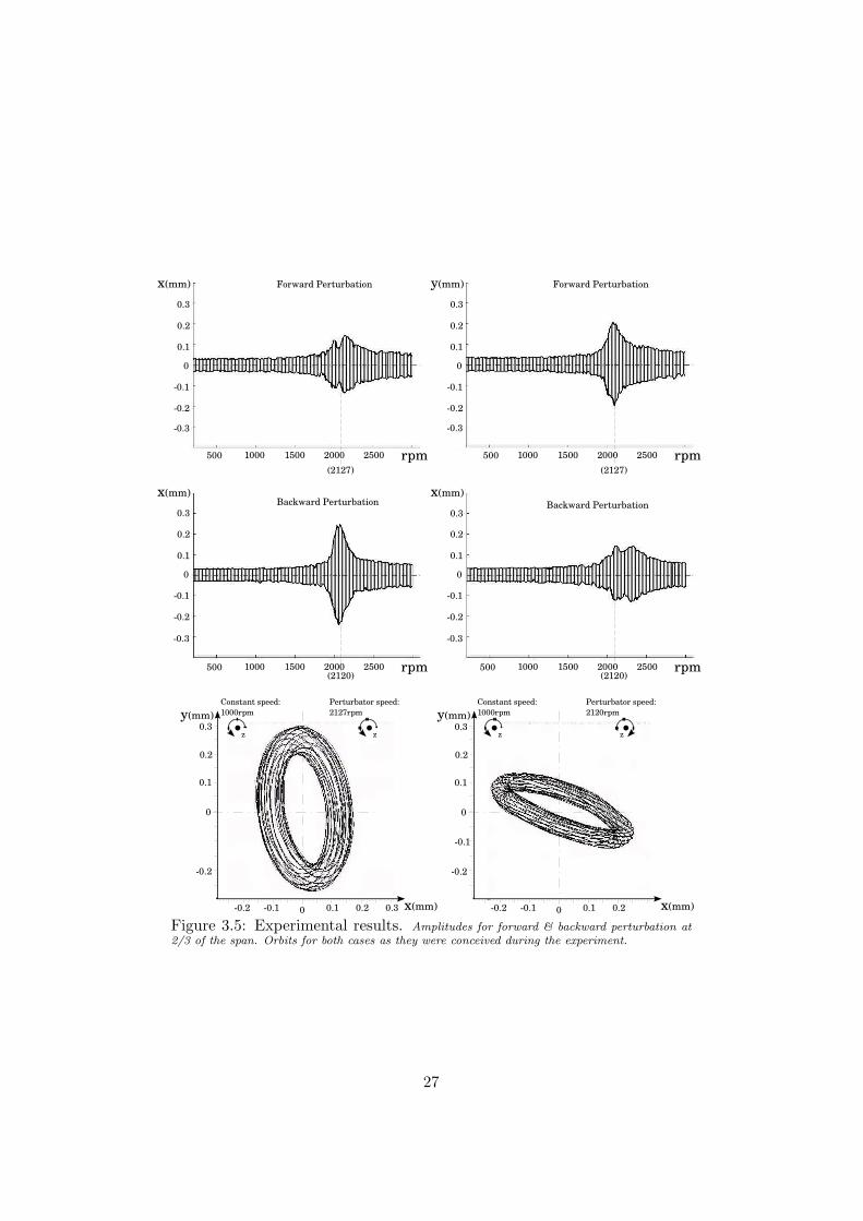
3.1.2 Disc mass at 2/3 of the span

The second experimental task is to displace the mass disc at the 2/3 ofthe span. The perturbation disc is as before very close to the mass discside towards the inboard bearing. All the experimental parameters for thisexperiment are the same with the experiment of Jeffcott rotor.

26

0

0.1

0.2

0.3

0.3

0.2

0.1

0

0.1

0.2

0.3

0.3

0.2

0.1

rpm

x(mm)

rpm

y(mm)

500 1000 1500 2000 2500 500 1000 1500 2000 2500

(2127) (2127)

00.2 0.1 0.1 0.2 0.3

•z •z



x(mm)

Forward Perturbation Forward Perturbation

0

•z •z



x(mm)

(2120)(2120)

Backward Perturbation Backward Perturbation

rpm500 1000 1500 2000 2500 rpm500 1000 1500 2000 2500

0

0.1

0.2

0.3

0.3

0.2

0.1

x(mm)

0

0.1

0.2

0.3

0.3

0.2

0.1

x(mm)

0.2 0.1 0.1 0.2

0.3

0.2

0.1

0

0.1

0.2

0.3

0.2

0.1

0

0.2

Figure 3.5: Experimental results. Amplitudes for forward & backward perturbation at2/3 of the span. Orbits for both cases as they were conceived during the experiment.

27

From the theory and since the mass is displaced, it is expected to havetwo different first critical speeds for back and fort perturbation. From Figure3.5 it is obvious that both cases give different critical speeds. Further more,the experimental result shows higher speed for forward perturbation, asit was expected. Thus, the first critical speed for forward perturbation isω ≈ 223rad/s and backward ω ≈ 222rad/s. In addition, it can be seen fromthe figure how the orbits in both cases become. At this point the orbits getthe highest amplitude, therefore, as it was mentioned in the previous sectionall rotating machines should pass as fast as possible through the first criticalarea.

These experiments were executed for speeds 200rpm-3000rpm. However,it can be seen that the orbits are getting smaller above 5000rpm. Thathappens due to the fact that the rotor gets stiffer while running in speedsmuch higher the first natural frequency. Further more, the shaft alwaysmoving in ellipsoid orbits(whirling) round the same imaginary axis even ifthe shaft changes amplitude.

a. b.

c.ω(rad/s)

ω(rad/s) ω(rad/s)

ω(rad/s) ω(rad/s)

Perturbation guide

Simple model Simple model & Bearings

Entire model & Bearings

(238)(231.5)

(231.4)

ω(rad/s)

(237) (231.0)

(230.8)

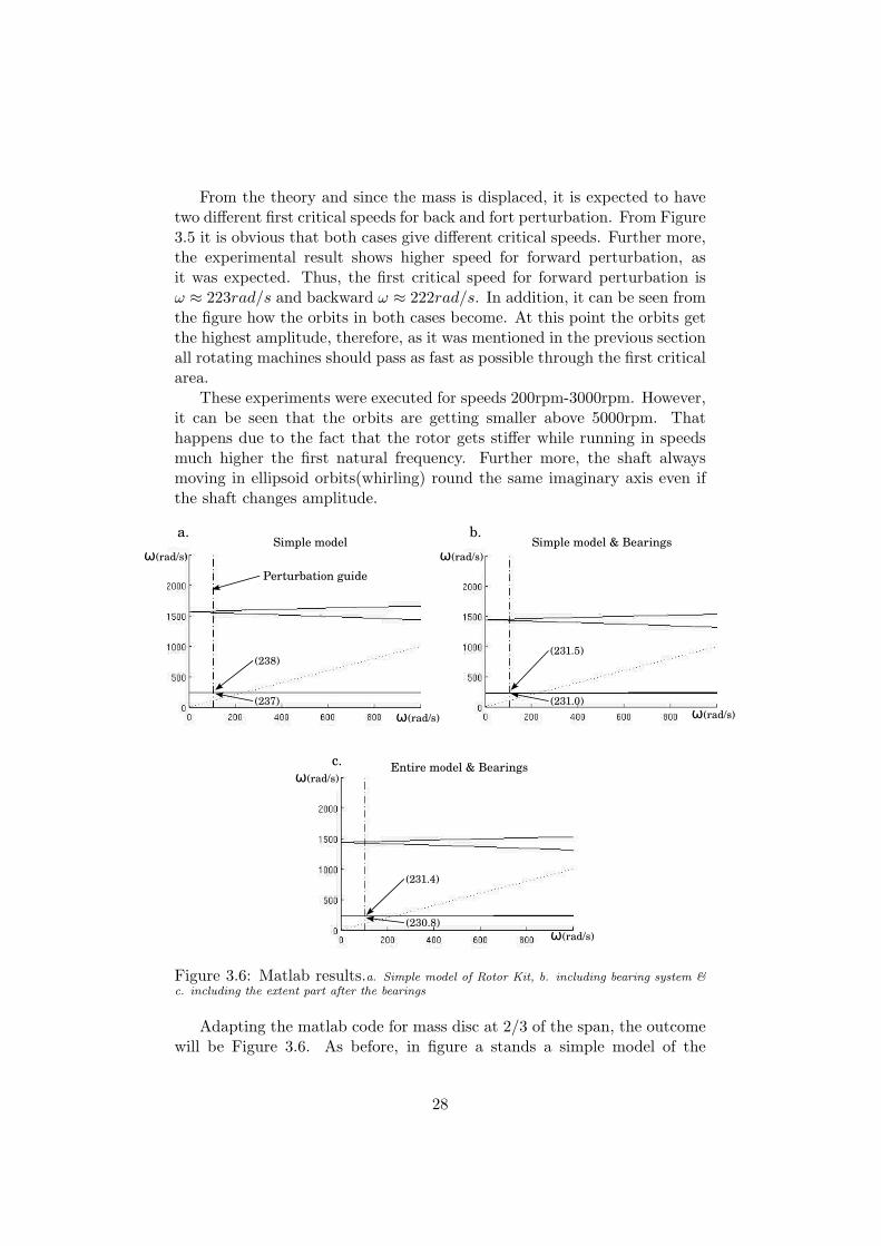
Figure 3.6: Matlab results.a. Simple model of Rotor Kit, b. including bearing system &c. including the extent part after the bearings

Adapting the matlab code for mass disc at 2/3 of the span, the outcomewill be Figure 3.6. As before, in figure a stands a simple model of the

28

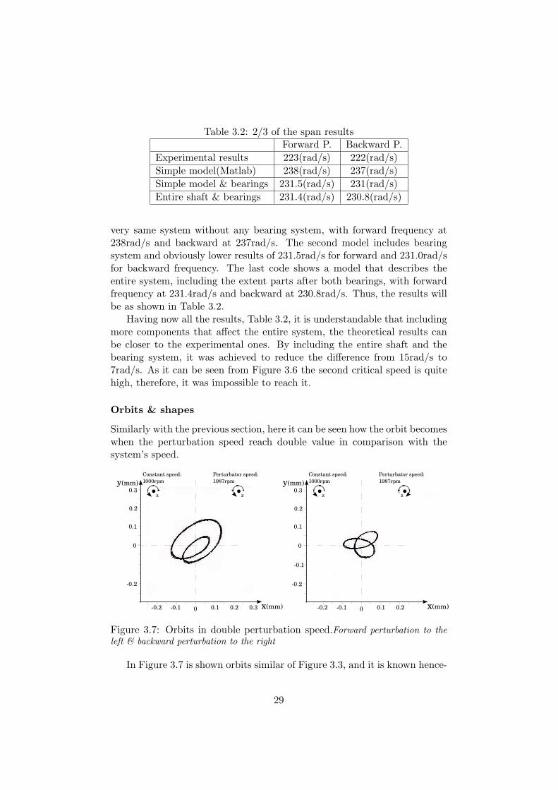
Table 3.2: 2/3 of the span resultsForward P. Backward P.

Experimental results 223(rad/s) 222(rad/s)Simple model(Matlab) 238(rad/s) 237(rad/s)Simple model & bearings 231.5(rad/s) 231(rad/s)Entire shaft & bearings 231.4(rad/s) 230.8(rad/s)

very same system without any bearing system, with forward frequency at238rad/s and backward at 237rad/s. The second model includes bearingsystem and obviously lower results of 231.5rad/s for forward and 231.0rad/sfor backward frequency. The last code shows a model that describes theentire system, including the extent parts after both bearings, with forwardfrequency at 231.4rad/s and backward at 230.8rad/s. Thus, the results willbe as shown in Table 3.2.

Having now all the results, Table 3.2, it is understandable that includingmore components that affect the entire system, the theoretical results canbe closer to the experimental ones. By including the entire shaft and thebearing system, it was achieved to reduce the difference from 15rad/s to7rad/s. As it can be seen from Figure 3.6 the second critical speed is quitehigh, therefore, it was impossible to reach it.

Orbits & shapes

Similarly with the previous section, here it can be seen how the orbit becomeswhen the perturbation speed reach double value in comparison with thesystem’s speed.

00.2 0.1 0.1 0.2 0.3

•z •z



x(mm) 0

•z •z



x(mm)0.2 0.1 0.1 0.2

0.3

0.2

0.1

0

0.1

0.2

0.3

0.2

0.1

0

0.2

Figure 3.7: Orbits in double perturbation speed.Forward perturbation to theleft & backward perturbation to the right

In Figure 3.7 is shown orbits similar of Figure 3.3, and it is known hence-

29

forth why the orbit change in these modes. Something interesting to be men-tioned, is that for speed multiple to the constant(three,four,five....times),these orbits will get proportionally one more sub-orbit. For instance, theorbits in the figure will get, one more sub-orbit for perturbation speed3000rpm,or two more sub-orbits for perturbation speed 4000rpm and sofort.

3.2 Journal bearing

Journal bearing is an option for observing different phenomena that occurswhile a shaft operates in an oil environment. Oil grows forces on a jour-nal surface in erratic orbits. In the following subsections is shown thosephenomena through different tasks by using Rotor Kit RK4 equipment.

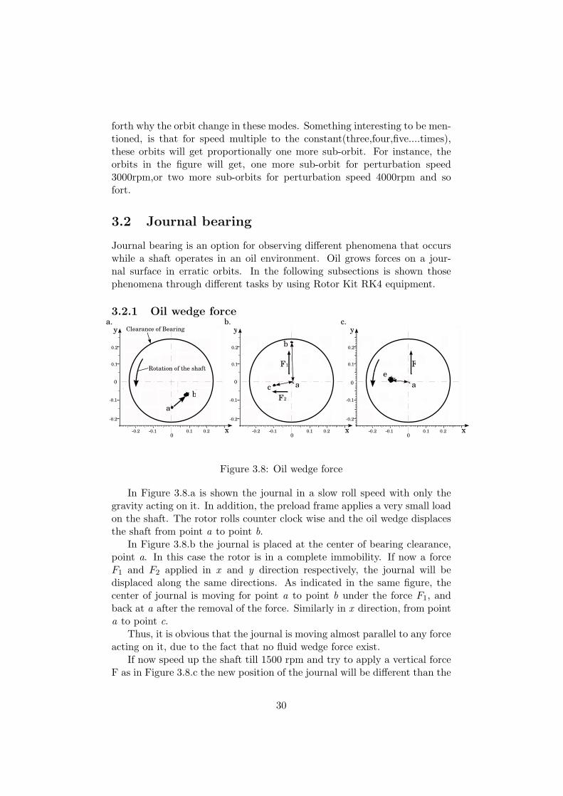
3.2.1 Oil wedge force

y

x0

0

Rotation of the shaft

a

b

y

x0

0 a

b

c

y

x0

0 ae

FF1

F2

Clearance of Bearinga. b. c.

0.1 0.20.10.2

0.1

0.2

0.1

0.2

0.2 0.20.1 0.10.1 0.10.2 0.2

0.2 0.2

0.1 0.1

0.1 0.1

0.2 0.2

Figure 3.8: Oil wedge force

In Figure 3.8.a is shown the journal in a slow roll speed with only thegravity acting on it. In addition, the preload frame applies a very small loadon the shaft. The rotor rolls counter clock wise and the oil wedge displacesthe shaft from point a to point b.

In Figure 3.8.b the journal is placed at the center of bearing clearance,point a. In this case the rotor is in a complete immobility. If now a forceF1 and F2 applied in x and y direction respectively, the journal will bedisplaced along the same directions. As indicated in the same figure, thecenter of journal is moving for point a to point b under the force F1, andback at a after the removal of the force. Similarly in x direction, from pointa to point c.

Thus, it is obvious that the journal is moving almost parallel to any forceacting on it, due to the fact that no fluid wedge force exist.

If now speed up the shaft till 1500 rpm and try to apply a vertical forceF as in Figure 3.8.c the new position of the journal will be different than the

30

expected one. Instead, the journal is moving in a new direction which is theresultant of force F and fluid wedge forces, point e. Thus, fluid forces canbe easily verified, since the applied force and the new direction is known.

3.3 Whirl & whip

x(mm)

y(mm)

x(mm) x(mm)

y(mm) y(mm)

0 0 00.1 0.1 0.10.1 0.20.2 0.2 0.20.1 0.10.2 0.2

0 0 0

0.2

0.1

0.1

0.2

0.2 0.2

0.1

0.1

0.2 0.2

0.1

0.1

Journal:700(rpm)6(psi)



0

0.2

0.1

0.1

0.2

y(mm)

0

0.2

0.1

0.1

0.2

y(mm)

0

0.2

0.1

0.1

0.2

y(mm)

0 0.10.1 0.20.2 0 0.10.1 0.20.2 0 0.10.1 0.20.2

Midspan:700(rpm)6(psi)



•z •z •z

•z•z •z

x(mm) x(mm) x(mm)

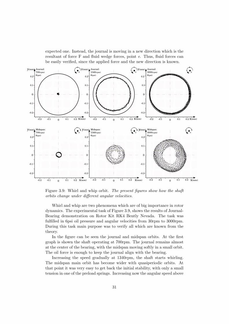
Figure 3.9: Whirl and whip orbit. The present figures show how the shaftorbits change under different angular velocities.

Whirl and whip are two phenomena which are of big importance in rotordynamics. The experimental task of Figure 3.9, shows the results of Journal-Bearing demonstration on Rotor Kit RK4 Bently Nevada. The task wasfulfilled in 6psi oil pressure and angular velocities from 30rpm to 3000rpm.During this task main purpose was to verify all which are known from thetheory.

In the figure can be seen the journal and midspan orbits. At the firstgraph is shown the shaft operating at 700rpm. The journal remains almostat the center of the bearing, with the midspan moving softly in a small orbit.The oil force is enough to keep the journal align with the bearing.

Increasing the speed gradually at 1340rpm, the shaft starts whirling.The midspan main orbit has become wider with quasiperiodic orbits. Atthat point it was very easy to get back the initial stability, with only a smalltension in one of the preload springs. Increasing now the angular speed above

31

1340rpm(which in fact is where the area of critical speed starts) and muchhigher of it(f.e 3000rpm) to make sure that the rotor is whipping, even thedouble tension was not able to stabilize the shaft in smooth operation. Fromthe picture can be seen how the orbit became at 3000rpm. In conclusion,it is more difficult to make the instability to go away while the rotor iswhipping.

Something that should be done comprehensible, is the difference betweenwhirl and whip. Whirl can take place sometimes even at low speeds, and itsfrequency is normally the half running speed(the oil film speed less than 50%of the journal surface speed, [12]). If this frequency coincides the naturalfrequency, then the oil whip occurs. Something remarkable is that whiplocks the shaft at the same orbit due to the high frequency, which is obviousfrom the experiments done with Rotor Kit. In addition, the fluid stiffnessis increasing due to lower circumferential velocity [11].

3.3.1 Oil pressure control

Oil pressure is very important to find out when the oil whirl/whip will takeplace. The oil pressure determines the size of concentrated radial forceswhich direct the journal.

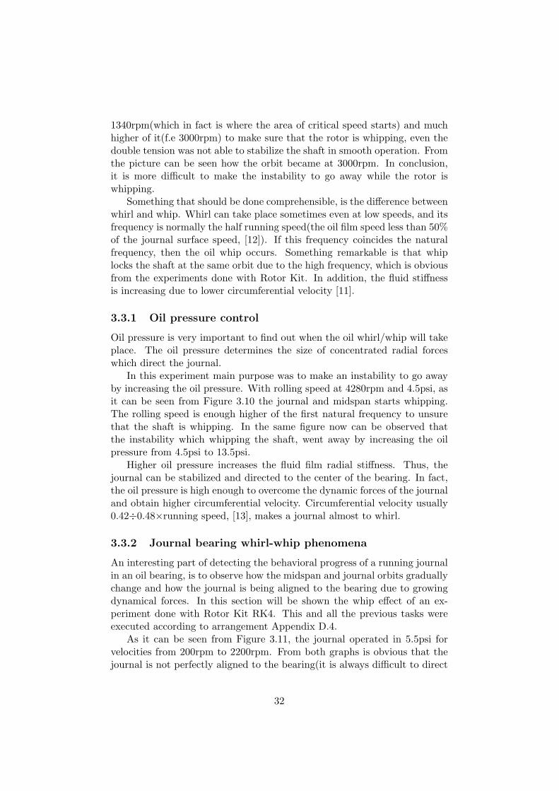
In this experiment main purpose was to make an instability to go awayby increasing the oil pressure. With rolling speed at 4280rpm and 4.5psi, asit can be seen from Figure 3.10 the journal and midspan starts whipping.The rolling speed is enough higher of the first natural frequency to unsurethat the shaft is whipping. In the same figure now can be observed thatthe instability which whipping the shaft, went away by increasing the oilpressure from 4.5psi to 13.5psi.

Higher oil pressure increases the fluid film radial stiffness. Thus, thejournal can be stabilized and directed to the center of the bearing. In fact,the oil pressure is high enough to overcome the dynamic forces of the journaland obtain higher circumferential velocity. Circumferential velocity usually0.42÷0.48×running speed, [13], makes a journal almost to whirl.

3.3.2 Journal bearing whirl-whip phenomena

An interesting part of detecting the behavioral progress of a running journalin an oil bearing, is to observe how the midspan and journal orbits graduallychange and how the journal is being aligned to the bearing due to growingdynamical forces. In this section will be shown the whip effect of an ex-periment done with Rotor Kit RK4. This and all the previous tasks wereexecuted according to arrangement Appendix D.4.

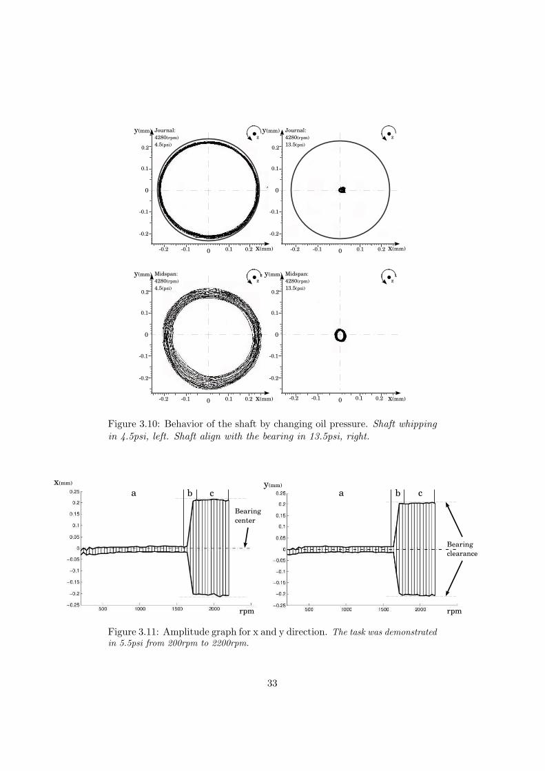
As it can be seen from Figure 3.11, the journal operated in 5.5psi forvelocities from 200rpm to 2200rpm. From both graphs is obvious that thejournal is not perfectly aligned to the bearing(it is always difficult to direct

32

x(mm)

y(mm)

x(mm)0 00.1 0.10.1 0.20.2 0.2 0.1 0.2

0 0

0.2

0.1

0.1

0.2

0.2

0.1

0.1

0.2

Journal:4280(rpm)4.5(psi)

Journal:4280(rpm)13.5(psi)

0

0.2

0.1

0.1

0.2

y(mm)

0

0.2

0.1

0.1

0.2

y(mm)

0 0.10.1 0.20.2 0 0.10.1 0.20.2

Midspan:4280(rpm)4.5(psi)

Midspan:4280(rpm)13.5(psi)

•z •z

•z•z

x(mm) x(mm)

y(mm)

Figure 3.10: Behavior of the shaft by changing oil pressure. Shaft whippingin 4.5psi, left. Shaft align with the bearing in 13.5psi, right.

rpm

x(mm) y(mm)

rpm rpm

a b c cba

Bearingcenter

Bearingclearance

Figure 3.11: Amplitude graph for x and y direction. The task was demonstratedin 5.5psi from 200rpm to 2200rpm.

33

a rolling journal at the right position.), thus, the journal is running in aneccentric position inside the bearing.

To begin with, each graph can be divided in three areas. The first areaa, as it can be seen from the graph, is the area where the journal is beingaligned gradually as the angular velocity is increasing. The journal increasesthe oil speed as well as the oil stiffness [11], as a result of changing positionin a new equilibrium area inside the bearing.

The second area b, is the area of oil whirl. The journal stars whirlingand rapidly is placed in higher orbit similar to the bearing’s clearance. Inthis area any instability can be easily disappeared with the application ofonly a small force, since the dynamic forces of the journal are still weak.

The last area c, is where the journal starts whipping. In fact, whip willlock whirl’s frequency and maintain it while operating into higher and higherspeeds [13]. According to [11] the shaft is in a very high position from thebearing center, therefore, a whipping shaft demands more force to stabilizeits orbit.

As can be seen from the figure, the axial line is the imaginary bearingcenter, and the dash lines the bearing clearance. It is obvious that thejournal will never exceed to have contact with the bearing surface due to oilwedge. It should be perfect lubrication, in order to avoid contact betweenthe journal and the bearing.

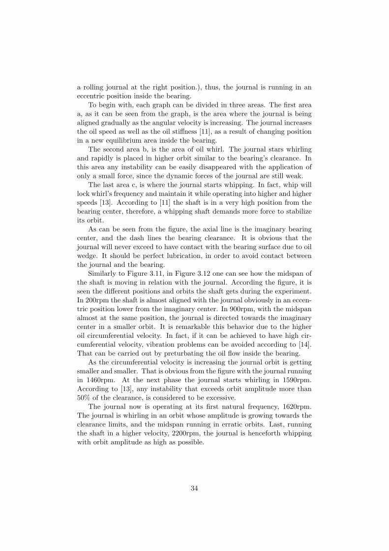
Similarly to Figure 3.11, in Figure 3.12 one can see how the midspan ofthe shaft is moving in relation with the journal. According the figure, it isseen the different positions and orbits the shaft gets during the experiment.In 200rpm the shaft is almost aligned with the journal obviously in an eccen-tric position lower from the imaginary center. In 900rpm, with the midspanalmost at the same position, the journal is directed towards the imaginarycenter in a smaller orbit. It is remarkable this behavior due to the higheroil circumferential velocity. In fact, if it can be achieved to have high cir-cumferential velocity, vibration problems can be avoided according to [14].That can be carried out by preturbating the oil flow inside the bearing.

As the circumferential velocity is increasing the journal orbit is gettingsmaller and smaller. That is obvious from the figure with the journal runningin 1460rpm. At the next phase the journal starts whirling in 1590rpm.According to [13], any instability that exceeds orbit amplitude more than50% of the clearance, is considered to be excessive.

The journal now is operating at its first natural frequency, 1620rpm.The journal is whirling in an orbit whose amplitude is growing towards theclearance limits, and the midspan running in erratic orbits. Last, runningthe shaft in a higher velocity, 2200rpm, the journal is henceforth whippingwith orbit amplitude as high as possible.

34

Journal:200(rpm)

5.5(psi)•z

Journal:900(rpm)

5.5(psi)• z

Journal:1460(rpm)

5.5(psi)•z

Midspan:200(rpm)

5.5(psi) •z

Midspan:900(rpm)

5.5(psi) •z

Midspan:1460(rpm)

5.5(psi) •z

Journal:1590(rpm)

5.5(psi)•z

Journal:1620(rpm)

5.5(psi)•z

Journal:2200(rpm)

5.5(psi)•z

Midspan:1590(rpm)

5.5(psi) •z

Midspan:1620(rpm)

5.5(psi) •z

Midspan:2200(rpm)

5.5(psi) •z

y(mm) y(mm)

y(mm)y(mm)y(mm)

y(mm) y(mm) y(mm)

y(mm) y(mm) y(mm)

x(mm) x(mm) x(mm)

x(mm)x(mm)x(mm)

x(mm) x(mm) x(mm)

x(mm)x(mm)x(mm)

y(mm)

0 00

0 0 0

000

0 0 0

0 0 0

000

0 0 0

000

0.2 0.2 0.2

0.20.20.2

0.2 0.2 0.2

0.20.20.2

0.2 0.2 0.2

0.20.20.2

0.1

0.1

0.1

0.1

0.1

0.1

0.1

0.1

0.1

0.1

0.1

0.1

0.2

0.1

0.1

0.2

0.1

0.1

0.2

0.1

0.1

0.2

0.1

0.1

0.2

0.1

0.1

0.2

0.1

0.1

0.10.10.2 0.2 0.1 0.1 0.2 0.1 0.1

0.2 0.1 0.10.2 0.1 0.10.2 0.1 0.1

0.2 0.1 0.1 0.2 0.1 0.1 0.2 0.1 0.1

0.2 0.1 0.10.2 0.1 0.10.2 0.1 0.1

Figure 3.12: Orbits of the journal and midspan.Behavior of the shaft for dif-ferent speeds running counter clockwise.

35

ConclusionThe present thesis reports all the experimental tasks done in order to com-pare and verify the analytical solution of a system. All the experimentaltasks were executed by using Rotor Kit RK4. The interesting part is, whytheoretical results do not match with the experimental.

First of all, in this thesis perturbation was of main importance and thatis why it was probed deep into it. From the experimental results it is seenthat all three theoretical model give higher first critical speeds. It is believedthat small errors as it can be seen from Table 3.1 and 3.2, can occur. ForJeffcott Rotor the error is: 5,58% for a simple model without bearings,3,61% for a model that includes bearing stiffness and 3,56% if it will betaken into account the extent parts out of the bearings. Similarly for Discmass at 2/3 of the span the error is: for a simple model 6,30% forward and6,33% backward, including the bearing stiffness 3,67% forward and 3,90%backward, and including the extent rotor length out the bearings 3,63%forward and 3,81% backward. It is natural to have some difference betweenthe theoretical and experimental results, since the theoretical method doesnot take in a consideration surrounding factors that can affect the finalresults. Besides, including only the bearing properties it can be realized thatthe error is very little. It is still unknown whether or not the friction at theattach points of the rotor(f.i the place where the disc is attached on the span)could change the physical properties of the rotor at that point, for instance,different stiffness of the rotor and damping due to the friction between therotor and the disc. Another potential factor for lower experimental firstnatural frequency, the transportation of vibrations from the motor via thecoupling.

Many of the reasons which have already been mentioned are: mistakesduring the calibration. For instance, the calibration and the values on whichthe program relies on, done under different conditions like, calibration envi-ronment and temperature. Further more, one more reason is that the chosenbearing stiffness was taken according to [5], however, even if the theoreticalmodel relied on this stiffness it is still not sure whether or not this valueis true. Thus, the bearing stiffness might be higher than the real one, andtherefore the theoretical model gives higher first critical speed.

In addition, the rotor’s body was considered to be rigid. In fact, allmembers of a system get some kind of distortion and obviously if someonedoes not include them in the final calculation, the result will be a stiffersystem.

Moreover, it has to be mentioned that Rotor Kit RK4 was adjusted on awooden bench whose potential weakness transfered vibrations on the mainsystem which met the first natural frequency earlier. The wooden benchadd some kind of elasticity on the system, something that was not takeninto account at the theoretical models.

36

Last but not least, it is understandable now that by making a modelthat describes exactly the real environment and situation in which a systemoperates, the approach can be closer. This is something difficult to make inreality, since the description of a real system becomes very complicate andmakes it difficult for engineers to compute such a model. Thus, from abovewe conclude that the assumptions gave us higher frequency.

In conclusion, the development of different experimental tasks broughtthe undergraduate students closer to the topic by raising questions andpoints that could be included at the present work or a nice suggestion forfuture research.

37

Appendix A

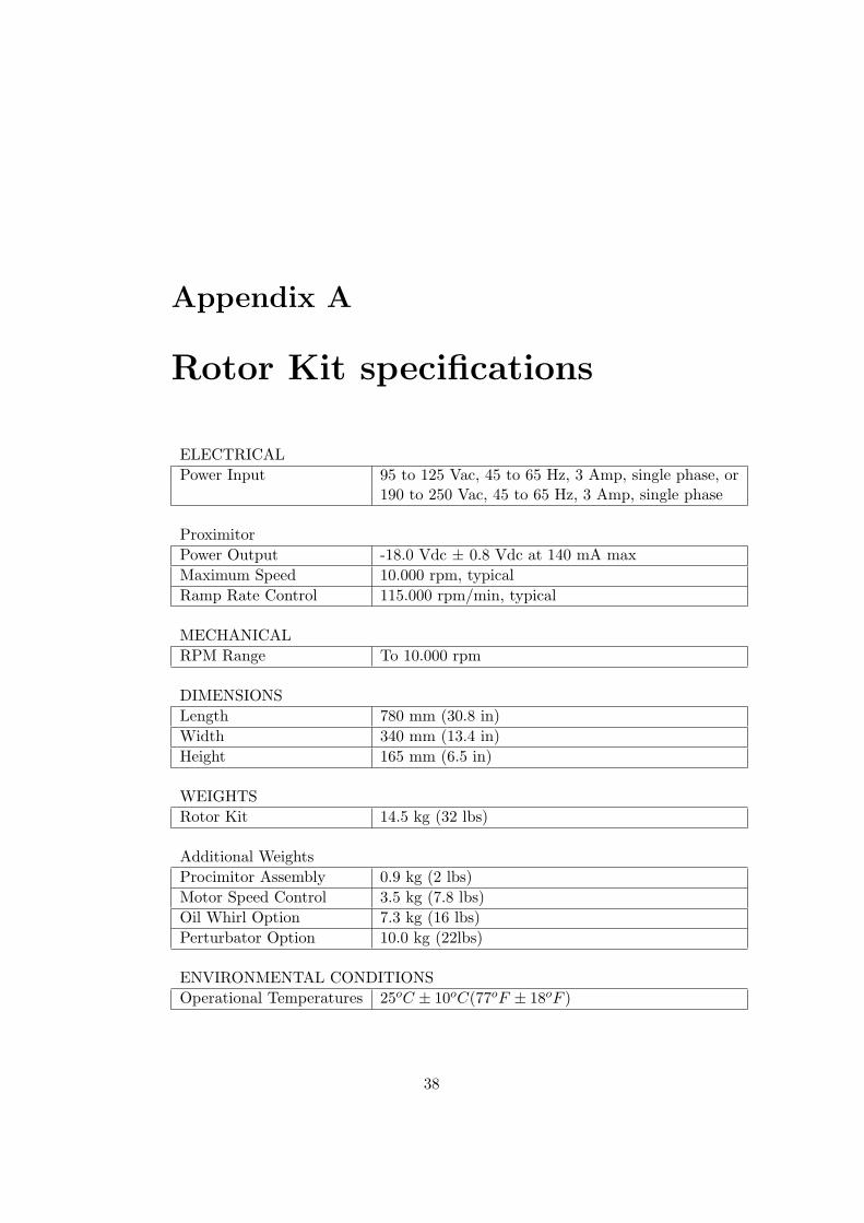
Rotor Kit specifications

ELECTRICALPower Input 95 to 125 Vac, 45 to 65 Hz, 3 Amp, single phase, or

190 to 250 Vac, 45 to 65 Hz, 3 Amp, single phase

ProximitorPower Output -18.0 Vdc ± 0.8 Vdc at 140 mA maxMaximum Speed 10.000 rpm, typicalRamp Rate Control 115.000 rpm/min, typical

MECHANICALRPM Range To 10.000 rpm

DIMENSIONSLength 780 mm (30.8 in)Width 340 mm (13.4 in)Height 165 mm (6.5 in)

WEIGHTSRotor Kit 14.5 kg (32 lbs)

Additional WeightsProcimitor Assembly 0.9 kg (2 lbs)Motor Speed Control 3.5 kg (7.8 lbs)Oil Whirl Option 7.3 kg (16 lbs)Perturbator Option 10.0 kg (22lbs)

ENVIRONMENTAL CONDITIONSOperational Temperatures 25oC ± 10oC(77oF ± 18oF )

38

Appendix B

Proximity probe

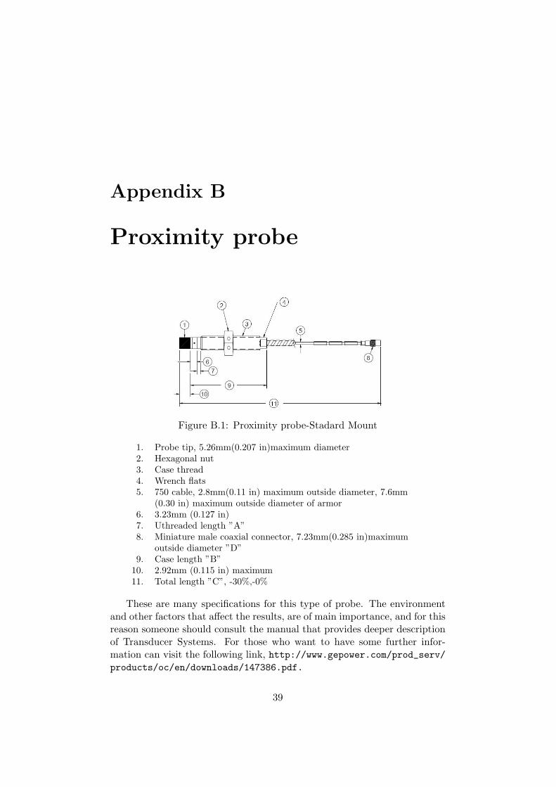
Figure B.1: Proximity probe-Stadard Mount

1. Probe tip, 5.26mm(0.207 in)maximum diameter2. Hexagonal nut3. Case thread4. Wrench flats5. 750 cable, 2.8mm(0.11 in) maximum outside diameter, 7.6mm

(0.30 in) maximum outside diameter of armor6. 3.23mm (0.127 in)7. Uthreaded length ”A”8. Miniature male coaxial connector, 7.23mm(0.285 in)maximum

outside diameter ”D”9. Case length ”B”

10. 2.92mm (0.115 in) maximum11. Total length ”C”, -30%,-0%

These are many specifications for this type of probe. The environmentand other factors that affect the results, are of main importance, and for thisreason someone should consult the manual that provides deeper descriptionof Transducer Systems. For those who want to have some further infor-mation can visit the following link, http://www.gepower.com/prod_serv/products/oc/en/downloads/147386.pdf.

39

Appendix C

High magnification extensometer calibrator

Instron Extensometer Calibrator.

Catalogue Numbers:2602-001(G-55-1)2602-004

(G-55-1M)

This instrument is a calibrator of high ration of output to displacement.Accurate and rugged units, this calibrator is adaptable to most types ofextensometers, and has a range of 1-inch(25,4mm-metric) units.

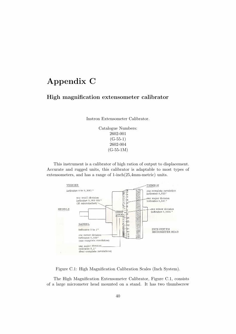
Figure C.1: High Magnification Calibration Scales (Inch System).

The High Magnification Extensometer Calibrator, Figure C.1, consistsof a large micrometer head mounted on a stand. It has two thumbscrew

40

couplings for mounting various size and shape adapter spindles suppliedwith the unit to accommodate most extensometers. The dial on the metricmicrometer head indicates directly to 0,002mm and by a four line vernier to0,0005mm. Its accuracy is ± 0,00038mm at any setting. Figure C.1 showsa vernier based in inch measuring system (The vernier that was used tocalibrate the probes was in metric system).

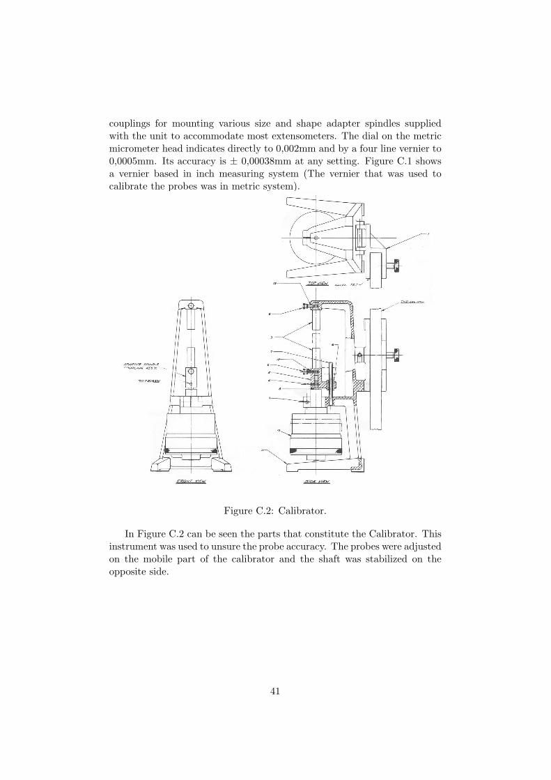
Figure C.2: Calibrator.

In Figure C.2 can be seen the parts that constitute the Calibrator. Thisinstrument was used to unsure the probe accuracy. The probes were adjustedon the mobile part of the calibrator and the shaft was stabilized on theopposite side.

41

Appendix D

Experimental suggestions

The present section introduces some experimental suggestions from BentlyNevada. Of course there are numerous combinations that someone can ac-complish on this equipment in order to achieve a more advanced model. Theexperimental models should be carried out with all the necessary instruc-tions for a proper environment. Something very crucial: be sure thatthe foundation on which Rotor Kit RK4 is accommodated, is rigid.

D.1 Disc & unbalance mass

a.

c.

b.

d.

αL

β α β

=α β

α βα β

γ

e

dThread holes for unbalance

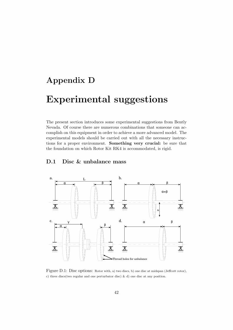
Figure D.1: Disc options: Rotor with, a) two discs, b) one disc at midspan (Jeffcott rotor),

c) three discs(two regular and one perturbator disc) & d) one disc at any position.

42

In Figure D.1 are indicated many disc configurations. As it can be seenin Figure D.1.a, one interesting arrangement is with two discs on the shaft.The discs can be placed in different positions along the shaft. The distancesα and β can be equal or not. Bently Nevada recommends α, β = 25% inrelation with the effective shaft length. In Figure D.1.b the disc is placedat the midspan, something interesting in case someone aims to work anddetect phenomena of Jeffcott rotor.

In Figure D.1.c there are three disc which according to Bently Nevada,a good suggestion is to use distance α, β = 25% and γ = 50% in relationwith the effective shaft length, or 12% and 50% respectively. The secondconfiguration is more preferable in case the bearings are not very stiff. Inthe present and all forth coming options an unbalance mass can be placed inorder to develop higher excitations in x and y direction. The unbalance masscan be easily placed/threaded on the discs, since each disc brings peripheralholes with thread as it is shown in Figure D.1.c.

The last configuration Figure D.1.d, a disc is placed at any position forfurther treatment. The distance can be chosen from the executor of thetask.

D.2 Preload condition

a. b.

Nylon rod

Preload springs

Preload springs

Contact surface

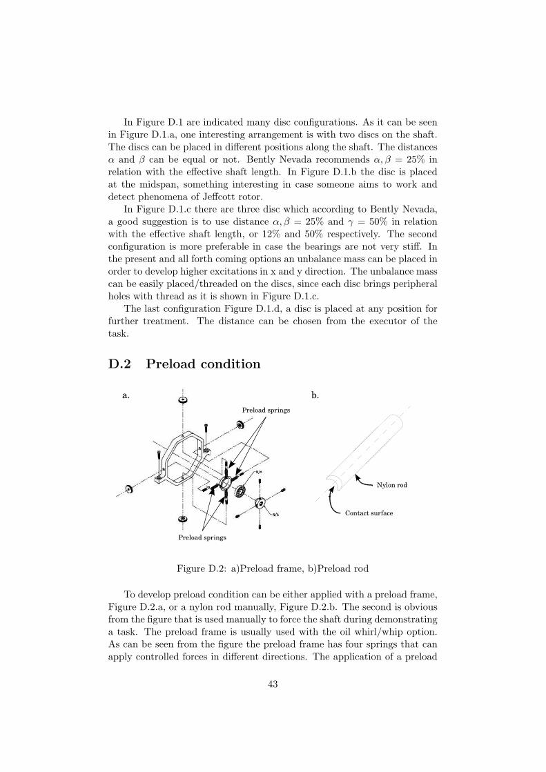
Figure D.2: a)Preload frame, b)Preload rod

To develop preload condition can be either applied with a preload frame,Figure D.2.a, or a nylon rod manually, Figure D.2.b. The second is obviousfrom the figure that is used manually to force the shaft during demonstratinga task. The preload frame is usually used with the oil whirl/whip option.As can be seen from the figure the preload frame has four springs that canapply controlled forces in different directions. The application of a preload

43

force is interesting task in showing how the shaft position and the orbitshape changes.

D.3 Rub condition

This task can be carried out by using a screw made out of copper whichcan be also called rub screw. The main purpose is to develop rub(friction)by adjusting the rub screw at the Probe Mount until it has surface contactwith the shaft.

D.4 Oil whirl/whip

25.6

25

25.40

300399

330

357

10.5

25.6

25

25.40

300399

331.5

357

10.5

Discs placed next to each otherNo gap between

Inboard bearing

kbear

kframe

Preload frame

Preload frame

(1)

(2)

(3)

(4)

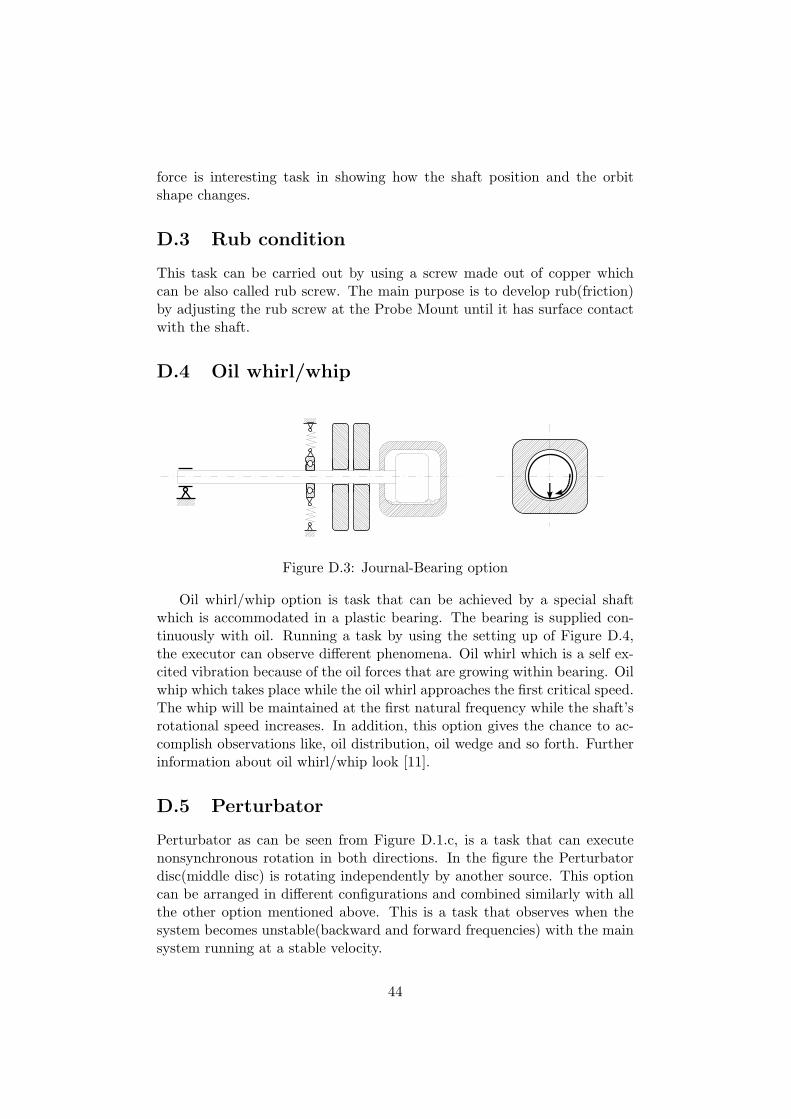
Figure D.3: Journal-Bearing option

Oil whirl/whip option is task that can be achieved by a special shaftwhich is accommodated in a plastic bearing. The bearing is supplied con-tinuously with oil. Running a task by using the setting up of Figure D.4,the executor can observe different phenomena. Oil whirl which is a self ex-cited vibration because of the oil forces that are growing within bearing. Oilwhip which takes place while the oil whirl approaches the first critical speed.The whip will be maintained at the first natural frequency while the shaft’srotational speed increases. In addition, this option gives the chance to ac-complish observations like, oil distribution, oil wedge and so forth. Furtherinformation about oil whirl/whip look [11].

D.5 Perturbator

Perturbator as can be seen from Figure D.1.c, is a task that can executenonsynchronous rotation in both directions. In the figure the Perturbatordisc(middle disc) is rotating independently by another source. This optioncan be arranged in different configurations and combined similarly with allthe other option mentioned above. This is a task that observes when thesystem becomes unstable(backward and forward frequencies) with the mainsystem running at a stable velocity.

44

Appendix E

Perturbation orbits

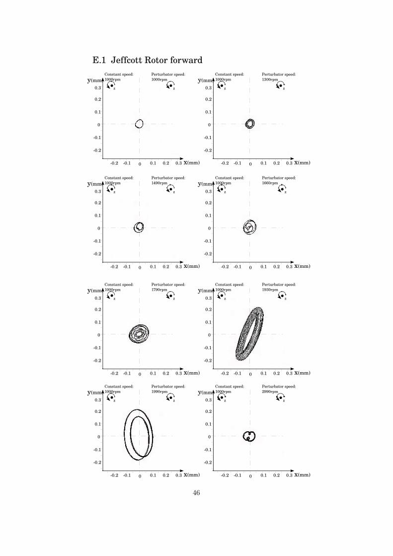
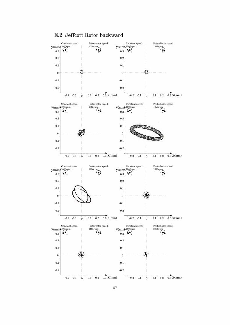
The following orbits were captured during the experimental task with per-turbator disc running in asynchronous rotational speed. The experimentswere accomplished for two configuration, one at the midspan(Jeffcott Rotor)and one at the 2/3 of the span. The experiments were executed for rotationalspeeds: constant speed 1000rpm and perturbator speed 200rpm÷3000rpm.

45

0

0

0.1

0.2

0.3

0.1

0.2

0.2 0.1 0.1 0.2 0.3

•z



x(mm) 0

0

0.1

0.2

0.3

0.1

0.2

0.2 0.1 0.1 0.2 0.3

•z



x(mm)

0

0

0.1

0.2

0.3

0.1

0.2

0.2 0.1 0.1 0.2 0.3

•z



x(mm) 0

0

0.1

0.2

0.3

0.1

0.2

0.2 0.1 0.1 0.2 0.3

•z



x(mm)

0

0

0.1

0.2

0.3

0.1

0.2

0.2 0.1 0.1 0.2 0.3

•z



x(mm) 0

0

0.1

0.2

0.3

0.1

0.2

0.2 0.1 0.1 0.2 0.3

•z



x(mm)

0

0

0.1

0.2

0.3

0.1

0.2

0.2 0.1 0.1 0.2 0.3

•z



x(mm) 0

0

0.1

0.2

0.3

0.1

0.2

0.2 0.1 0.1 0.2 0.3

•z



x(mm)

•z•z

•z •z

•z•z

•z •z

E.1 Jeffcott Rotor forward

46

0

0

0.1

0.2

0.3

0.1

0.2

0.2 0.1 0.1 0.2 0.3

•z



x(mm) 0

0

0.1

0.2

0.3

0.1

0.2

0.2 0.1 0.1 0.2 0.3

•z •zConstant speed:1000rpm


x(mm)

0

0

0.1

0.2

0.3

0.1

0.2

0.2 0.1 0.1 0.2 0.3

•z



x(mm) 0

0

0.1

0.2

0.3

0.1

0.2

0.2 0.1 0.1 0.2 0.3



x(mm)

0

0

0.1

0.2

0.3

0.1

0.2

0.2 0.1 0.1 0.2 0.3

•z



x(mm) 0

0

0.1

0.2

0.3

0.1

0.2

0.2 0.1 0.1 0.2 0.3



x(mm)

0

0

0.1

0.2

0.3

0.1

0.2

0.2 0.1 0.1 0.2 0.3

•z



x(mm) 0

0

0.1

0.2

0.3

0.1

0.2

0.2 0.1 0.1 0.2 0.3



x(mm)

•z

•z

•z

•z

E.2 Jeffcott Rotor backward

47

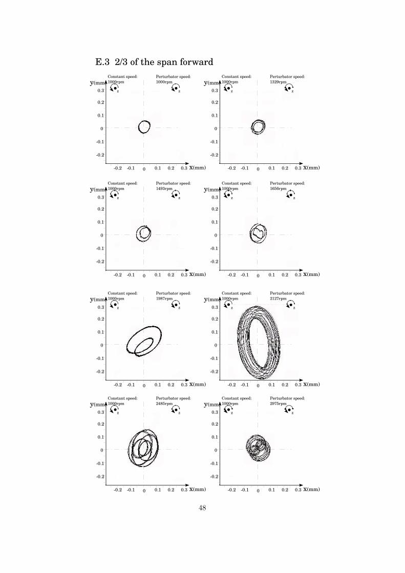
0

0

0.1

0.2

0.3

0.1

0.2

0.2 0.1 0.1 0.2 0.3

•z



x(mm) 0

0

0.1

0.2

0.3

0.1

0.2

0.2 0.1 0.1 0.2 0.3

•z



x(mm)

0

0

0.1

0.2

0.3

0.1

0.2

0.2 0.1 0.1 0.2 0.3

•z



x(mm) 0

0

0.1

0.2

0.3

0.1

0.2

0.2 0.1 0.1 0.2 0.3

•z



x(mm)

0

0

0.1

0.2

0.3

0.1

0.2

0.2 0.1 0.1 0.2 0.3

•z



x(mm) 0

0

0.1

0.2

0.3

0.1

0.2

0.2 0.1 0.1 0.2 0.3

•z



x(mm)

0

0

0.1

0.2

0.3

0.1

0.2

0.2 0.1 0.1 0.2 0.3

•z



x(mm) 0

0

0.1

0.2

0.3

0.1

0.2

0.2 0.1 0.1 0.2 0.3

•z



x(mm)

•z•z

•z •z

•z•z

•z •z

E.3 2/3 of the span forward

48

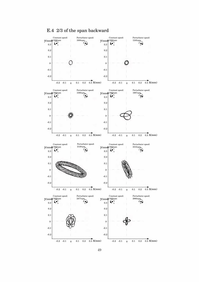
0

0

0.1

0.2

0.3

0.1

0.2

0.2 0.1 0.1 0.2 0.3

•z



x(mm) 0

0

0.1

0.2

0.3

0.1

0.2

0.2 0.1 0.1 0.2 0.3



x(mm)

0

0

0.1

0.2

0.3

0.1

0.2

0.2 0.1 0.1 0.2 0.3

•z



x(mm) 0

0

0.1

0.2

0.3

0.1

0.2

0.2 0.1 0.1 0.2 0.3



x(mm)

0

0

0.1

0.2

0.3

0.1

0.2

0.2 0.1 0.1 0.2 0.3

•z



x(mm) 0

0

0.1

0.2

0.3

0.1

0.2

0.2 0.1 0.1 0.2 0.3



x(mm)

0

0

0.1

0.2

0.3

0.1

0.2

0.2 0.1 0.1 0.2 0.3

•z



x(mm) 0

0

0.1

0.2

0.3

0.1

0.2

0.2 0.1 0.1 0.2 0.3



x(mm)

•z

•z

•z

•z

E.4 2/3 of the span backward

49

Bibliography

[1] Kari Tammi. Active vibration control of rotor in desktop test environ-ment. PhD thesis, VTT, Technical Research Centre of Finland, April2003.

[2] Xi Wu Jim Meagher and Chris Lencioni. Response of a warped fleciblerotor with a fluid bearing. International Journal of Rotating Machinery,2008(147653):9, June 2007.

[3] Tomas Lukas Petr Ferfecki, Jan Ondrouch. Investigation of vibrationof a rotor system supported by absolutely rigid bearings with a shaftcontaining a notch. Technical report, Technical university of Ostrava,2006.

[4] Agnes Muszynska. Oil whip of a rotor supported in a poorly lubricatedbearing. Technical report, Bently Nevada, 1998.

[5] Enayet Halim. Experiment design for simulating different faults in a ro-tor kit. Technical report, Chemical and Materials Engineering Depart-ment University of Alberta,Edmonton, AB, Canada, T6G2G6, JUNE2005.

[6] M. Paterno P. Forte and E. Rustighi. A magnetorheological fluiddamper for rotor applications. International Journal of Rotating Ma-chinery, 2004:8, January 2003.

[7] Jan-Olov Aidanpaa. M7010T dynamics in mechanical systems, fem instructural dynamics-lucture notes. LTU.

[8] Ronald D.Ziemian William McGuire, Richard H.Gallagher. Matrixstructural analysis. John Wiley & Sons, Inc, 605 Third Avenue, NewYork, NY 10158-0012, 2nd edition, 2000.

[9] ANDREW DIMAROGONAS. Vibration for Engineers. A PearsonEducation Company, PRENTICE HALL, Upper Saddle River, NewJersey 07458, 2nd edition, 1996.

[10] Jan-Olov Aidanpaa. M7010T dynamics in mechanical systems, rotordynamics-lucture notes. LTU.

50

[11] Bently Nevada Asset Condition Monitoring, 1631 Bently ParkwaySouth Minden, Nevada USA 89423, USA. Operation Manual RotorKit Oil Whirl/Whip Option Model RK4, 11 2007.

[12] Agnieszka(Agnes) Muszyska. Rotordynamics. Taylor & Francis Group,6000 Broken Sound Parkway NW, Suite 300, Boca Raton, FL 33487-2742, 1st edition, 2005.

[13] Cornelius Scheffer and Paresh Girdhar. Machinery Vibration Analysis& Predictive Maintenance. Elsevier Linacre House, Jordan Hill, OxfordOX2 8DP 200 Wheeler Road, Burlington, MA 01803, JUL-2004.

[14] John J. McKetta. Encyclopedia of Chemical Processing and Desgn.MARCEL DEKKER, INC. 270 Madison Avenue, New York, New York,10016, 1996.

51

Documents

Analyses of a Rotor Dynamic Testrigs - DiVA portal1029066/FULLTEXT01.pdfChapter 1 Rotor dynamic modeling and analysis 1.1 Element matrices This section will describe the theoretical