Embed Size (px)
Citation preview

i
ANALYICAL STUDY TO INVESTIGATE THE SEISMIC
PERFORMANCE OF SINGLE STORY TILT-UP
STRUCTURES
by
OMRI OLUND
P. Eng, B.Sc. Civil Engineering, University of British Columbia, 2001
A THESIS SUBMITTED IN PARTIAL FULFILMENT OF
THE REQUIREMENTS FOR THE DEGREE OF
MASTER OF APPLIED SCIENCE
in
THE FACULTY OF GRADUATE STUDIES
(Civil Engineering)
THE UNIVERSITY OF BRITISH COLUMBIA
April 2009
© Omri Olund, 2009
ii
ABSTRACT
This report describes an analytical study to investigate the seismic performance of single-story
tilt-up structures with steel deck roof diaphragms. A review of current practice in North America
for the seismic design of tilt-up structures reveals two points of interest; the flexibility of the roof
diaphragm is not considered in calculation of the fundamental building period for the design, and
that a force-based approach is used for seismic design that does not incorporate the principles of
capacity-design currently used in other building systems, such as moment frames, braced frames,
and shear walls.
To explore the application of capacity design for tilt-up structures, three possible failure
mechanisms are investigated and compared: rocking of wall panels, sliding of wall panels, and
frame action for buildings with wall panels incorporating large openings. Based on results of an
industry survey, two building archetypes are created to represent the most common building
types found in seismically active areas; one including solid panels and the second incorporating
panels with large openings. Consideration of the sliding mechanism suggests it would be
difficult to incorporate into common applications due to building geometry irregularities,
difficulties in estimating sliding resistance, and permanent deformation resulting from the
mechanism.
Analytical results from this study are compared with findings from previous research; the most
interesting comparison showed the period from the analytical model to be within 10% of the
estimated building period from ASCE 41 when the weight of the out-of-plane walls are
considered in the estimate.
The rocking mechanism and frame mechanism are studied further by carrying out a preliminary
assessment of seismic performance factors (R-values) utilizing concepts from the ATC-63
Methodology. Various analyses, including non-linear time history analyses for a suite of
earthquakes, are carried out on 3D models of the building archetypes. Based on analysis results,
the adequacies of some building components are evaluated, including the strength of the roof

iii
deck connectors and the strength of wall panel to roof connections both in-plane and out-of-
plane. Further research is required to provide a recommendation for R-values, however,
preliminary recommendations are provided and limitations of the study are discussed.

iv
TABLE OF CONTENTS
Abstract ......................................................................................................................... ii
Table of Contents ........................................................................................................ iv
List of Tables ............................................................................................................... ix
List of Figures ............................................................................................................... x
Acknowledgements ................................................................................................... xiv
1 INTRODUCTION ..................................................................................................... 1
1.1 Overview ............................................................................................................................................................. 1
1.2 Current Practice in the Design of Tilt-up Structures ..................................................................................... 4
1.2.1 Design of Tilt-up Panels for Vertical and Out-of-Plane Loading............................................................... 4
1.2.2 Design of Tilt-up Panels for In-Plane Loading .......................................................................................... 7
1.2.3 Design of Connections ............................................................................................................................. 11
1.2.4 Connecting Panels for Vertical, Out-of-Plane and In-Plane Loads .......................................................... 14
1.2.5 Design of Roof System ............................................................................................................................ 22
1.2.6 U.S. Perspective ....................................................................................................................................... 25
1.2.7 Discussion of Current Design Methods.................................................................................................... 26
1.3 Previous Research ............................................................................................................................................ 27
1.3.1 Roof Diaphragm ....................................................................................................................................... 27
1.3.2 Wall Panels with Openings ...................................................................................................................... 31
1.3.3 Building System ....................................................................................................................................... 33

Table of Contents
v
1.4 Research Aims.................................................................................................................................................. 35
1.4.1 Evaluate Previous Research on Building System ..................................................................................... 35
1.4.2 Investigate Alternatives for Capacity Design ........................................................................................... 35
1.4.3 Quantify Building Performance for Selected Mechanisms ...................................................................... 36
1.4.4 Thesis Organization ................................................................................................................................. 36
2 ASSESSMENT METHODOLOGY ........................................................................ 37
2.1 General ............................................................................................................................................................. 37
2.2 Seismic Performance Factors ......................................................................................................................... 39
2.3 Seismic Hazard ................................................................................................................................................ 40
2.3.1 Ground Motion Record Sets ..................................................................................................................... 40
2.3.2 Ground Motion Record Scaling ............................................................................................................... 42
2.4 Archetypical Systems....................................................................................................................................... 44
2.4.1 Archetypical System 1: Solid Wall Panels ............................................................................................... 48
2.4.2 Archetypical System 2: Wall Panels with Openings ................................................................................ 50
2.5 Non-linear Analysis Methods .......................................................................................................................... 51
2.5.1 Software ................................................................................................................................................... 51
2.5.2 Simulated and Non-Simulated Deterioration / Collapse Mechanisms ..................................................... 52
2.5.3 Non-linear Model Calibration .................................................................................................................. 53
2.5.4 Incremental Dynamic Analysis ................................................................................................................ 54
2.6 Collapse Fragility and Uncertainties .............................................................................................................. 56
2.7 Median Collapse Adjustment for Spectral Shape ......................................................................................... 57
2.8 Evaluation and Acceptance Criteria .............................................................................................................. 58
3 INVESTIGATION OF MECHANISM ALTERNATIVES ......................................... 60
Table of Contents
vi
3.1 Analysis Model Configuration ........................................................................................................................ 60
3.1.1 Conventional Building ............................................................................................................................. 60
3.1.2 Model 1: Sliding Mechanism ................................................................................................................... 62
3.1.3 Model 2: Rocking Mechanism ................................................................................................................. 65
3.1.4 Model 3: Frame Mechanism .................................................................................................................... 65
3.2 Model Verification ........................................................................................................................................... 67
3.2.1 Model 1: Sliding Mechanism ................................................................................................................... 67
3.2.2 Model 2: Rocking Mechanism ................................................................................................................. 71
3.2.3 Model 3: Frame Mechanism .................................................................................................................... 75
3.3 Time History Analysis Results ........................................................................................................................ 80
3.3.1 Model 1: Sliding Mechanism ................................................................................................................... 81
3.3.2 Model 2: Rocking Mechanism ................................................................................................................. 82
3.3.3 Model 3: Frame Mechanism .................................................................................................................... 84
3.4 IDA Results ...................................................................................................................................................... 87
3.4.1 Model 1: Sliding Mechanism ................................................................................................................... 87
3.4.2 Model 2: Rocking Mechanism ................................................................................................................. 88
3.4.3 Model 3: Frame Mechanism .................................................................................................................... 89
3.5 Comparison of Rocking and Sliding Mechanisms ........................................................................................ 90
3.6 Possible Connection Details for Rocking Mechanism................................................................................... 91
3.7 Incorporating a Rocking Mechanism for Panels with Openings ................................................................. 97
3.8 Evaluation of Previous Research .................................................................................................................. 100
3.8.1 Ductility Demands of Walls vs. Roof .................................................................................................... 100
3.8.2 Ductility Demands on Legs of Frame Panels ......................................................................................... 101
3.8.3 Seismic Demands on Roof Diaphragm Due to Out-of-Plane Response of Wall Panels ........................ 102
4 QUANTIFICATION OF SEISMIC PERFORMANCE FACTORS ......................... 105

Table of Contents
vii
4.1 Model 4: Rocking Mechanism ...................................................................................................................... 105
4.1.1 Simulated and Non-Simulated Collapse ................................................................................................. 108
4.1.2 IDA Results, Collapse Statistics and Uncertainty .................................................................................. 109
4.1.3 Acceptance Criteria and Evaluation of R ............................................................................................... 113
4.2 Model 5: Frame Mechanism ......................................................................................................................... 115
4.2.1 Simulated and Non-Simulated Collapse ................................................................................................. 116
4.2.2 IDA Results, Collapse Statistics and Uncertainty .................................................................................. 116
4.2.3 Acceptance Criteria and Evaluation of R ............................................................................................... 119
4.3 Model 6: Frame Mechanism – Eccentric Building ..................................................................................... 121
4.3.1 Simulated and Non-Simulated Collapse ................................................................................................. 122
4.3.2 IDA Results, Collapse Statistics and Uncertainty .................................................................................. 122
4.3.3 Acceptance Criteria and Evaluation of R ............................................................................................... 126
4.3.4 Comparison of IDA Results from Rocking, Frame and Eccentric Models ............................................ 127
5 CONCLUSIONS AND RECOMMENDATIONS ................................................... 130
5.1 Summary of Observations ............................................................................................................................ 130
5.2 Recommendations and Future Research ..................................................................................................... 134
6 REFERENCES .................................................................................................... 137
APPENDIX A. ANALYSIS OF CONVENTIONAL BUILDING .................................... 142
APPENDIX B. DESIGN NOTES AND MODEL PROPERTIES FOR ARCHETYPICAL
SYSTEM 1: SOLID WALL PANELS .......................................................................... 165
APPENDIX C. DESIGN NOTES AND MODEL PROPERTIES FOR ARCHETYPICAL
SYSTEM 2: PANELS WITH OPENINGS ................................................................... 197

Table of Contents
viii
APPENDIX D. SAMPLE CALCULATION FOR COLLAPSE STATISTICS FOR
ARCHETYPICAL SYSTEM 1: SOLID WALL PANELS ............................................. 216

ix
LIST OF TABLES
Table 1.1 Deck Test Specimens – Fastening Configurations (Essa, Tremblay and Rogers 2003)
...................................................................................................................................................... 29
Table 1.2 Results from Monotonic Testing (Essa, Tremblay and Rogers, 2003) ...................... 29
Table 1.3 Results from Cyclic Testing (Essa, Tremblay and Rogers 2003)............................... 30
Table 2.1 Summary of Ground Motion Records (ATC-63, 2008) .............................................. 41
Table 2.2 Industry Survey Results – Typical Single Story Tilt-up Building Attributes.............. 45
Table 2.3 Spectral Shape Factor for Different R Factors ............................................................ 58
List of Figures
x
LIST OF FIGURES
Figure 1.1 Concrete Tilt-up Wall Panels Ready for Concrete Placement ..................................... 2
Figure 1.2 2005 NBCC Design Spectrum ..................................................................................... 9
Figure 1.3 Standard Tilt-up Connectors ...................................................................................... 13
Figure 1.4 Joist Pocket Connection - EM1 (Weiler Smith Bowers, 2008) ................................. 16
Figure 1.5 Tie Strut Connection for Out-of-Plane Deck Forces (Weiler Smith Bowers, 2008) . 16
Figure 1.6 Slab to Panel Connection (Weiler Smith Bowers, 2008) ........................................... 17
Figure 1.7 Panel on Dropped Footing (Weiler Smith Bowers, 2008) ......................................... 18
Figure 1.8 Deck Connection for In-Plane Forces (Weiler Smith Bowers, 2008) ........................ 19
Figure 1.9 Design Forces for Panel Sliding / Overturning .......................................................... 19
Figure 1.10 Design Forces for Roof Diaphragm ......................................................................... 23
Figure 1.11 Schematic of Test Setup ........................................................................................... 28
Figure 1.12 Monotonic and Quasistatic Cyclic Loading Protocols ............................................. 28
Figure 1.13 Panel Geometry ........................................................................................................ 31
Figure 1.14 Test Specimen Reinforcement ................................................................................. 32
Figure 2.1 Seismic Performance Factors - Canadian Practice ..................................................... 39
Figure 2.2 Seismic Performance Factors - US Practice ............................................................... 40
Figure 2.2 IDA Results for Different Scaling Procedures ........................................................... 43
Figure 2.3 Typical Roof Design for All Building Archetypes .................................................... 47
Figure 2.4 Roof Diaphragm Zones .............................................................................................. 48
Figure 2.5 Solid Wall Panels – Concrete Outline, Reinforcement, and Connections ................. 49
List of Figures
xi
Figure 2.6 Wall Panels with Openings – Concrete Outline, Reinforcement, and Connections .. 51
Figure 2.7 IDA Results for One Earthquake Record ................................................................... 54
Figure 2.8 IDA Results for Five Earthquake Records ................................................................. 55
Figure 2.9 Fragility Curve Based on IDA Results for 22 Earthquake Records ........................... 56
Figure 3.1 Two-Panel Model for Pushover Analyses .................................................................. 61
Figure 3.2 Model Used to Investigate Sliding System ................................................................ 63
Figure 3.3 Model Used to Investigate Frame Mechanism ........................................................... 66
Figure 3.4 First Mode (Period = 0.58 seconds) ........................................................................... 68
Figure 3.5 Sliding Mechanism - Pushover Analysis Along Short Axis of Building ................... 69
Figure 3.6 Sliding Mechanism – Displaced Shape for Pushover Along Short Axis of Building 70
Figure 3.7 Sliding Mechanism - Pushover Analysis Along Long Axis of Building ................... 71
Figure 3.8 Rocking Mechanism - Pushover Analysis Along Short Axis of Building ................. 72
Figure 3.9 Rocking Mechanism – Displaced Shape for Pushover Along Short Axis of Building
...................................................................................................................................................... 73
Figure 3.10 Rocking Mechanism - Pushover Analysis Along Long Axis of Building ............... 74
Figure 3.11 Frame Mechanism – Force-Displacement Plot for Beam-Column Subassembly:
Comparison of Analytical and Experimental Results (Dew et al., 2001) ..................................... 76
Figure 3.12 Frame Mechanism – Panel Leg with Geometry and Reinforcement from
Archetypical System 2: (a)Force-Displacement Plot (b)Perform Model of Leg ......................... 77
Figure 3.13 Frame Mechanism – Two Legs Connected vs. One Leg: (a)Moment-Curvature Plot;
(b)Force-Drift Plot ........................................................................................................................ 79
Figure 3.14 Frame Mechanism – Pushover Analysis Along Short Building Axis ...................... 80
Figure 3.15 Sliding Model – Wall and Roof Drifts for Northridge Earthquake; (a) Sa(T1)=0.1g;
(b) Sa(T1)=1.0g ............................................................................................................................ 81
Figure 3.16 Sliding Model – Breakdown of Energy Dissipation ................................................ 82

List of Figures
xii
Figure 3.17 Rocking Model – Wall and Roof Drifts for Northridge Earthquake, Sa(T1)=1.0g . 83
Figure 3.18 Rocking Model – Breakdown of Energy Dissipation .............................................. 84
Figure 3.19 Frame Model – Wall and Roof Drifts for Northridge Earthquake, Sa(T1)=3.0g .... 85
Figure 3.20 Frame Model – Breakdown of Energy Dissipation .................................................. 86
Figure 3.21 Sliding Model – IDA Drift Results for 8 Ground Motion Records: (a)End Walls;
(b)Centre of Roof .......................................................................................................................... 87
Figure 3.22 Rocking Model – IDA Drift Results for 8 Ground Motion Records: (a)End Walls;
(b)Centre of Roof .......................................................................................................................... 89
Figure 3.23 Frame Model – IDA Drift Results for 8 Ground Motion Records: (a)End Walls;
(b)Centre of Roof .......................................................................................................................... 90
Figure 3.24 Sliding and Rocking Models: IDA Drift Results for 8 Ground Motion Records:
(a)End Walls; (b)Centre of Roof ................................................................................................. 91
Figure 3.25 Rocking Mechanism – Consideration at Panel to Panel Interface - Elevation View
from Inside of Building ................................................................................................................ 92
Figure 3.26 Rocking Mechanism – Consideration at Panel to Panel Interface - Detail at Panel
Interface ........................................................................................................................................ 93
Figure 3.27 Rocking Mechanism – Possible Connection Details: Elevation of Building ........... 95
Figure 3.28 Rocking Mechanism – Possible Base Connection Details: Tie-down and Shear Pin
...................................................................................................................................................... 96
Figure 3.27 Rocking Mechanism for Panels with Openings – Possible Connection Details:
(a)Elevation of Building; (b)Details ............................................................................................. 99
Figure 3.28 Median Drift Centre of Roof and End Walls for 8 Ground Motion Records:
(a)Sliding Model; (b)Rocking Model ......................................................................................... 100
Figure 3.29 Inelastic Wall Displacement at Sa(T1) = 3.0g: Analysis Results vs. Predicted .... 102
List of Figures
xiii
Figure 3.32 Seismic Demands on Roof Diaphragm due to Out-of-Plane Response of Wall
Panels for Sa(T1) = 0.5g: Analysis Results vs. Common North American Practice vs. ASCE41-
06 Approximation ....................................................................................................................... 103
Figure 4.1 Rocking Model – 2 Adjacent Panels Connected at End Walls ................................ 106
Figure 4.2 Rocking Model - Pushover Analysis Along Short Axis of Building (2 panels
connected) ................................................................................................................................... 107
Figure 4.3 Rocking Model – IDA Results for 22 Ground Motion Record Pairs: (a)Drift at End
Wall; (b)Drift at Centre of Roof; (c)In-Plane Deck Forces at End Walls; (d)Out-of-Plane Wall to
Roof Connection Forces ............................................................................................................. 110
Figure 4.4 Rocking Model – Collapse Statistics: (a)Roof Drift; (b)In-Plane Deck Forces; (c)Out-
of-Plane Deck Forces .................................................................................................................. 113
Figure 4.5 Frame Model – IDA Results for 22 Ground Motion Record Pairs: (a)Drift at End
Wall; (b)Drift at Centre of Roof; (c)In-Plane Deck Forces at End Walls; (d)Out-of-Plane Wall to
Roof Connection Forces ............................................................................................................. 117
Figure 4.6 Frame Model – Collapse Statistics: (a)Roof Drift; (b)In-Plane Deck Forces; (c)Out-
of-Plane Deck Forces .................................................................................................................. 119
Figure 4.7 Eccentric Model – IDA Results for 22 Ground Motion Record Pairs: (a)Drift at End
Wall; (b)Drift at Centre of Roof ................................................................................................ 123
Figure 4.8 Eccentric Model – IDA Results for 22 Ground Motion Record Pairs: (a)In-Plane
Deck Forces at End Wall with Frame Panels; (b) In-Plane Deck Forces at End Wall with Solid
Panels; (c) Out-of-Plane Deck Forces ........................................................................................ 124
Figure 4.9 Eccentric Model – Collapse Statistics: (a)Roof Drift; (b)In-Plane Deck Forces;
(c)Out-of-Plane Deck Forces ...................................................................................................... 126
Figure 4.10 Comparison of IDA Results for the Rocking Model, Frame Model, and Eccentric
Model: (a)Drift at End Walls with Openings; (b)Drift at Centre of Roof (c)In-Plane Deck Forces;
(d) Out-of-Plane Deck Forces ..................................................................................................... 128

xiv
ACKNOWLEDGEMENTS
My sincerest thanks go to my research supervisor, Dr. Ken Elwood, for his guidance and support
throughout this research endeavour. Thanks also to Dr. Perry Adebar, for his insight and for
completing second review duties.
I would also like to acknowledge the generous support of the Portland Cement Association and
the Cement Association of Canada which provided funding to the author. Support and input
from Kevin Lemieux of Weiler Smith Bowers is also greatly appreciated.

1
1 INTRODUCTION
1.1 Overview
Tilt-up construction is widely used in the United States and Canada to construct warehouses,
office buildings, schools and other types of buildings. Use of the tilt-up method of construction
began in the 1940’s as a way of constructing concrete wall buildings with considerably less
formwork than is necessary for casting the walls in place, thus offering cost advantages over
other types of construction. Other advantages include the durability of the concrete walls in
comparison with other types of walls and the efficiency of the system in that the concrete walls
act as cladding, vertical load carrying elements, and as components of the lateral load resisting
system (LLRS). The most common application of tilt-up construction is for single story
commercial and industrial structures.
Until recently, the design of tilt-up structures was not specifically considered in Canadian
building and material codes. Canadian codes first addressed the design of tilt-up structures in the
Design of Concrete Structures Standard issued in 1994, CAN/CSA A23.3-94 (CSA 1994).
Currently, tilt-up structures in Canada are designed in accordance with the requirements of the
2005 National Building Code of Canada (NBCC) and the Design of Concrete Structures
Standard CAN/CSA A23.3-04. The Concrete Design Handbook, Third Edition (CAC 2006)
offers some guidance and examples for the design of tilt-up structures. In the latter publication,
within Section 13, titled “Tilt-up Concrete Wall Panels”, the following is stated:
“Further development of this design standard is required in areas including:
• Service Load Deflections
• Analysis and Design for Seismic Requirements ”
Considering their extensive use in seismically active areas, there has been limited research into
the seismic performance of tilt-up building systems, and most of the research that has been
Chapter 1 Introduction
2
conducted on this topic has focussed on tilt-up buildings with timber deck diaphragms
(Hamburger and McCormick, 1994).
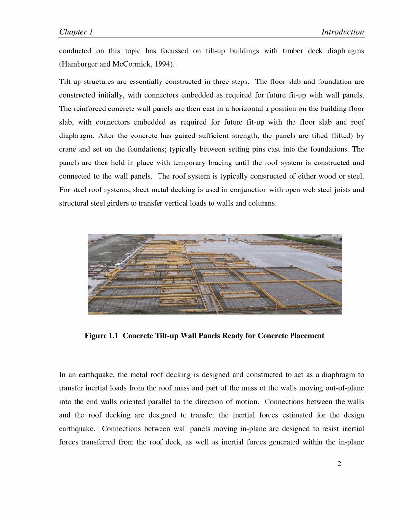
Tilt-up structures are essentially constructed in three steps. The floor slab and foundation are
constructed initially, with connectors embedded as required for future fit-up with wall panels.
The reinforced concrete wall panels are then cast in a horizontal a position on the building floor
slab, with connectors embedded as required for future fit-up with the floor slab and roof
diaphragm. After the concrete has gained sufficient strength, the panels are tilted (lifted) by
crane and set on the foundations; typically between setting pins cast into the foundations. The
panels are then held in place with temporary bracing until the roof system is constructed and
connected to the wall panels. The roof system is typically constructed of either wood or steel.
For steel roof systems, sheet metal decking is used in conjunction with open web steel joists and
structural steel girders to transfer vertical loads to walls and columns.
Figure 1.1 Concrete Tilt-up Wall Panels Ready for Concrete Placement
In an earthquake, the metal roof decking is designed and constructed to act as a diaphragm to
transfer inertial loads from the roof mass and part of the mass of the walls moving out-of-plane
into the end walls oriented parallel to the direction of motion. Connections between the walls
and the roof decking are designed to transfer the inertial forces estimated for the design
earthquake. Connections between wall panels moving in-plane are designed to resist inertial
forces transferred from the roof deck, as well as inertial forces generated within the in-plane
Chapter 1 Introduction
3
walls themselves, such that there is a sufficient margin of safety against sliding or overturning.
For a building designed in accordance with current practices, it is difficult to determine in what
manner failure of the system will occur for lateral loads. The roof diaphragm and the wall
connections are designed using similar force modification factors (R-values), leading to
uncertainty as to whether the roof deck or the wall connections would yield first. Also, some of
the wall connections, specifically the connections between the walls and the floor slab and
footing, are subject to both lateral loads and uplift when a lateral load is applied to the building.
Although the wall to slab connections have been tested for lateral loads, there have been no tests
for uplift. In order to accurately predict the behaviour of these connections, it is necessary to
understand the strength and stiffness interactions that exist for combined uplift and lateral loads.
Experimental testing was carried out on these connections as part of this study in order to
investigate these interactions. A detailed description of the testing program and results is
provided in Frank Devine’s Master’s Thesis (Devine, 2008)
The portion of the research discussed herein consists of an analytical study to investigate the
seismic performance of single-story tilt-up structures with steel deck roof diaphragms. Some of
the possible failure mechanisms for these structures are investigated and compared, including
rocking of wall panels, sliding of wall panels, and frame action for wall panels with openings.
The rocking mechanism and frame mechanism are studied further by incorporating them into the
design of a typical single story tilt-up structure designed and assessing the performance of the
structure by utilizing concepts from the ATC-63 Methodology (ATC, 2008),
The sections below include a brief review of current practices in the design of tilt-up structures, a
discussion of previous related research, research aims, and guidelines used to form the basis for
the research methodology. Also included are a detailed description of the research methodology,
the specific building systems studied and associated analytical models, results from analyses
conducted, as well as some conclusions and recommendations based on the study.
Chapter 1 Introduction
4
1.2 Current Practice in the Design of Tilt-up Structures
1.2.1 Design of Tilt-up Panels for Vertical and Out-of-Plane Loading
In CAN/CSA A23.3-04, tilt-up panels are described in Clause 23.1.3 as “slender vertical flexural
slabs that resist lateral wind or seismic loads and are subject to very low axial stresses.” This
clause also states, “Because of their high slenderness ratios, they shall be designed for second-
order P-∆ effects to ensure structural stability and satisfactory performance under specified
loads.”
Tilt-up concrete wall panels are designed as load bearing elements that span vertically from the
floor slab to the roof. Panels are designed to resist vertical loads imposed by the roof system.
Typically, for the purposes of wall panel design, loads from roof joists are considered as
uniformly distributed line loads applied at an eccentricity to the centreline of the panel. A
minimum eccentricity of half the panel thickness is prescribed by the code to account for
accidental bearing irregularities.
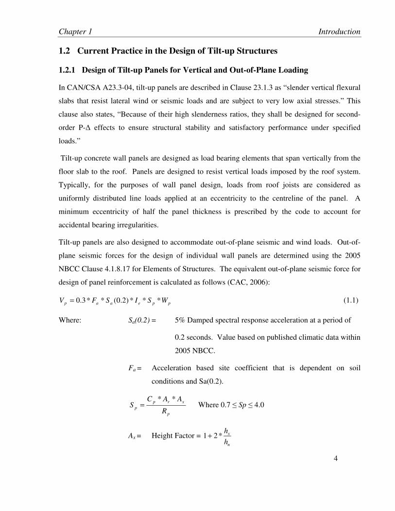
Tilt-up panels are also designed to accommodate out-of-plane seismic and wind loads. Out-of-
plane seismic forces for the design of individual wall panels are determined using the 2005
NBCC Clause 4.1.8.17 for Elements of Structures. The equivalent out-of-plane seismic force for
design of panel reinforcement is calculated as follows (CAC, 2006):
ppeaap WSISFV ***)2.0(**3.0= (1.1)
Where: Sa(0.2) = 5% Damped spectral response acceleration at a period of
0.2 seconds. Value based on published climatic data within
2005 NBCC.
Fa = Acceleration based site coefficient that is dependent on soil
conditions and Sa(0.2).
p
xrp
pR
AACS
**= Where 0.7 ≤ Sp ≤ 4.0
Ax = Height Factor = n
x
h
h*21+
Chapter 1 Introduction
5
hx, ,hn = Height above the base level. For out-of-plane forces, hx is taken
as the center of mass of the panel.
Ie = Importance factor for earthquakes, equals 1.0 for normal
importance buildings.
Wp = Weight of panel
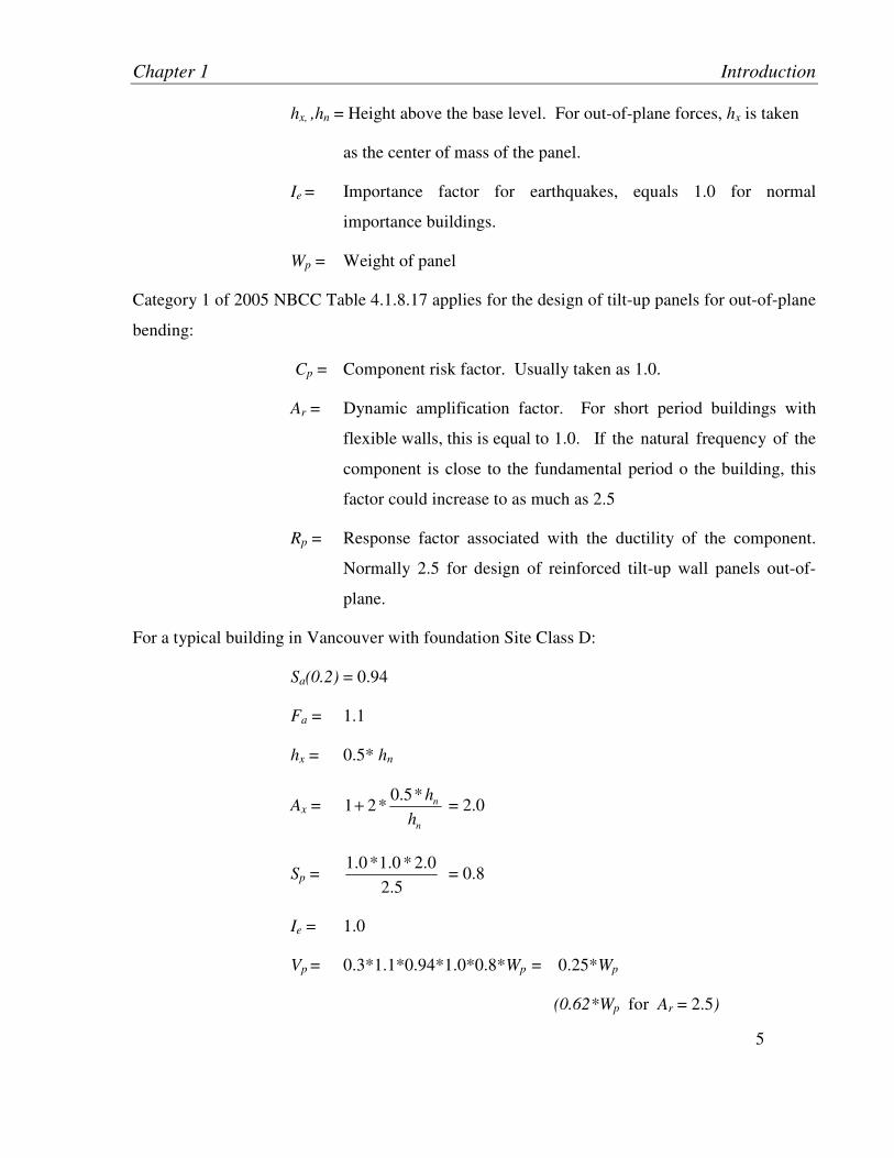
Category 1 of 2005 NBCC Table 4.1.8.17 applies for the design of tilt-up panels for out-of-plane
bending:
Cp = Component risk factor. Usually taken as 1.0.
Ar = Dynamic amplification factor. For short period buildings with
flexible walls, this is equal to 1.0. If the natural frequency of the
component is close to the fundamental period o the building, this
factor could increase to as much as 2.5
Rp = Response factor associated with the ductility of the component.
Normally 2.5 for design of reinforced tilt-up wall panels out-of-
plane.
For a typical building in Vancouver with foundation Site Class D:
Sa(0.2) = 0.94
Fa = 1.1
hx = 0.5* hn
Ax = n
n
h
h*5.0*21+ = 2.0
Sp = 5.2
0.2*0.1*0.1 = 0.8
Ie = 1.0
Vp = 0.3*1.1*0.94*1.0*0.8*Wp = 0.25*Wp
(0.62*Wp for Ar = 2.5)
Chapter 1 Introduction
6
Although the value of Ar is normally taken as 1.0, it is important to note that if the flexibility of
the deck diaphragm is considered, the fundamental period of the building may approach the
fundamental period of the wall panels, resulting in considerably greater amplification of seismic
demands in the wall panels. Often, out-of-plane seismic loads will exceed wind pressure.
Out-of-plane wind loads for the design of wall panels are determined based on the 2005 NBCC
Clause 4.1.7 for Wind Loads. Appendix A includes an example of the design of a typical tilt-up
building, including the design of panels for out-of-plane wind and seismic loads.
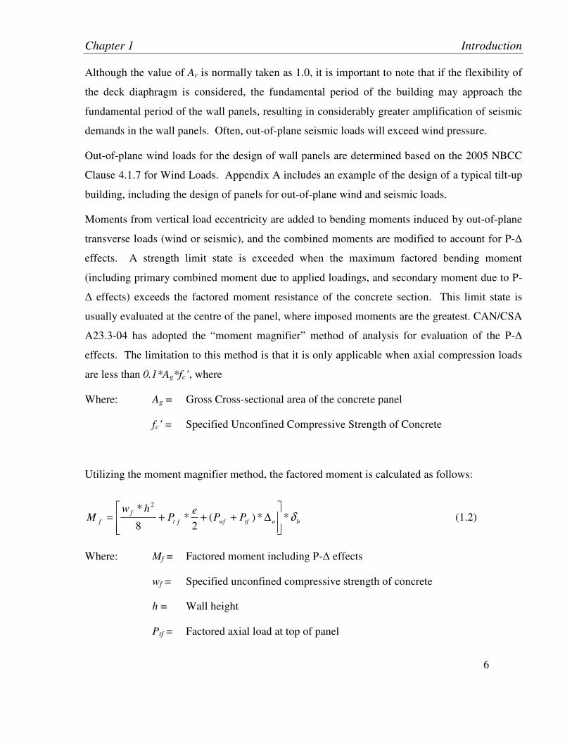
Moments from vertical load eccentricity are added to bending moments induced by out-of-plane
transverse loads (wind or seismic), and the combined moments are modified to account for P-∆
effects. A strength limit state is exceeded when the maximum factored bending moment
(including primary combined moment due to applied loadings, and secondary moment due to P-
∆ effects) exceeds the factored moment resistance of the concrete section. This limit state is
usually evaluated at the centre of the panel, where imposed moments are the greatest. CAN/CSA
A23.3-04 has adopted the “moment magnifier” method of analysis for evaluation of the P-∆
effects. The limitation to this method is that it is only applicable when axial compression loads
are less than 0.1*Ag*fc’, where
Where: Ag = Gross Cross-sectional area of the concrete panel
fc’ = Specified Unconfined Compressive Strength of Concrete
Utilizing the moment magnifier method, the factored moment is calculated as follows:
botfwfft
f
f PPe
Phw
M δ**)(2
*8
* 2
∆+++= (1.2)
Where: Mf = Factored moment including P-∆ effects
wf = Specified unconfined compressive strength of concrete
h = Wall height
Ptf = Factored axial load at top of panel

Chapter 1 Introduction
7
e = Axial load eccentricity at top of panel
Pwf = Factored panel weight above mid height
∆o = Initial deflection at panel mid height
δb = Moment magnification factor
The moment magnification factor,
fb
f
b
K
P−
=
1
1δ
Where: Pf = Factored axial load at mid height = Ptf + Pwf
Kbf = Panel bending stiffness =2*5
**48
h
IE crc
Ec = Concrete elastic modulus
Icr = Cracked section moment of inertia
Appendix B includes an example of the design of a typical tilt-up building, with P-∆ effects
considered utilizing the method described above.
There is also a limitation on the panel height to thickness ratio, depending on the reinforcement
configuration used in the cross-section. For a single mat of reinforcement, the maximum height
to thickness ratio is 50; for a double mat, the maximum is 65.
In addition to the above, CAN/CSA A23.3 also states that transverse deflections due to non-
seismic service loads must be less than h/100.
The NBCC 2005 requires that interstory drift due to seismic loading must be smaller than 2.5%
drift. This design requirement is not considered in the Concrete Design Handbook.
1.2.2 Design of Tilt-up Panels for In-Plane Loading
The main sources of in-plane loads for tilt-up wall panels are wind and seismic loads. As for
out-of-plane loads, wind loads are calculated in accordance with the 2005 NBCC Clause 4.1.7 on
Wind Loads.
Chapter 1 Introduction
8
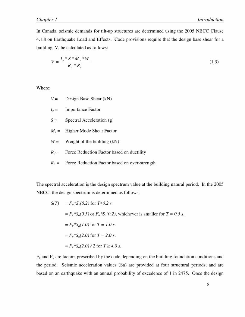
In Canada, seismic demands for tilt-up structures are determined using the 2005 NBCC Clause
4.1.8 on Earthquake Load and Effects. Code provisions require that the design base shear for a
building, V, be calculated as follows:
od
ve
RR
WMSIV
*
***=
(1.3)
Where:
V = Design Base Shear (kN)
Ie = Importance Factor
S = Spectral Acceleration (g)
Mv = Higher Mode Shear Factor
W = Weight of the building (kN)
Rd = Force Reduction Factor based on ductility
Ro = Force Reduction Factor based on over-strength
The spectral acceleration is the design spectrum value at the building natural period. In the 2005
NBCC, the design spectrum is determined as follows:
S(T) = Fa*Sa(0.2) for T≤0.2 s
= Fv*Sa(0.5) or Fa*Sa(0.2), whichever is smaller for T = 0.5 s.
= Fv*Sa(1.0) for T = 1.0 s.
= Fv*Sa(2.0) for T = 2.0 s.
= Fv*Sa(2.0) / 2 for T ≥ 4.0 s.
Fa and Fv are factors prescribed by the code depending on the building foundation conditions and
the period. Seismic acceleration values (Sa) are provided at four structural periods, and are
based on an earthquake with an annual probability of excedence of 1 in 2475. Once the design

Chapter 1 Introduction
9
spectrum is constructed, spectral accelerations for structure periods between the values provided
can be interpolated from the design spectrum. Figure 1.2 below illustrates the design spectrum
for Vancouver for a site with a very dense soil or soft rock foundation (Site Class C, Fa=1,
Fv=1):
Figure 1.2 2005 NBCC Design Spectrum
Most tilt-up structures satisfy the code requirements for “Regular Structures” and as such,
seismic demands are evaluated using the “Equivalent Static Force Procedure”. In addition, for
regular structures with an Rd value greater than or equal to 1.5, the base shear can be reduced as
follows:
od
e
RR
WSIV
*
*)2.0(*
3
2∗=
(1.4)
The 2/3 cutoff is illustrated in Figure 1.1 above.
For various types of buildings, the 2005 NBCC code prescribes formulae to calculate the period
to be used in determining the spectral acceleration. Of the building types considered in the code,

Chapter 1 Introduction
10
a tilt-up building most closely resembles a concrete shear wall building. The formula provided
to calculate the fundamental period for a concrete shear wall building is as follows:
43
*05.0 hT = (1.5)
Where:
h = height of the shear wall in meters
For a typical wall panel with a height of 9 m, Eqn. 1.5 would give a period of vibration equal to
0.26 seconds. It is interesting to note that for a typical tilt-up structure, the period calculated in
accordance with the 2005 NBCC code can be substantially shorter than the 1st mode period
results from an eigenvalue analysis of a typical single story tilt-up building with a steel deck
diaphragm. This discrepancy will be discussed further in Section 3.2.
The higher mode shear factor, Mv, is equal to unity for buildings with a fundamental period
smaller than 1.0 seconds. This factor is included to account for the effect of higher modes on the
response of the structure, and does not apply for relatively short buildings with a small period.
The weight of the building, W, used in determining the base shear typically consists of the roof
weight, including 25% of the design snow load, the full dead weight of the in-plane walls, and
half the weight of the out-of-plane walls. Only half the weight of the out-of-plane walls is
considered since the behaviour of the walls in the out-of-plane direction is assumed to be similar
to simply supported beams subjected to a uniformly distributed load, i.e. half the inertial force is
assumed to be transferred to the base of the panel, and half is assumed to be transferred to the
diaphragm.
For the design of tilt-up structures, the force reduction factor based on ductility, Rd, varies
between 1.0 and 1.5 depending on the component being designed. An Rd value of 1.5 is used for
tilt-up structures for calculation of the base shear. The force reduction factor based on over-
strength, Ro, is1.3, consistent with the NBCC 2005 requirements for conventional construction.
Chapter 1 Introduction
11
1.2.3 Design of Connections
In tilt-up construction, vertical and lateral loads are transferred to the wall panels and between
panels by various types of connections. For tilt-up structures within the scope of this work,
connections are used to transfer gravity loads from beams and joists to the panels, lateral forces
between the roof deck diaphragm and the panels, shear forces between panels, shear forces
between the panels and the floor slab or foundation.
The design of connections for tilt-up structures is carried out in accordance with conventional
design practices for embedded connections. Guidelines for the design of tilt-up connections are
provided within the Concrete Design Handbook (CAC 2006) for Canadian practice, and within
“Connections for Tilt-up Wall Construction” (PCA 1987) for design in the United States. The
descriptions provided below of typical practice in the design and construction of tilt-up
connections are based on information from the guideline documents referenced above.
Connections are designed to resist forces greater than the imposed loads. Typical connections
used in the tilt-up industry are cast-in-place concrete in-fill anchors, drilled-in anchors, and
welded embedded metal connectors.
Cast-in-place concrete in-fill sections are constructed by leaving a blockout between the panels
to be connected and extending the panel rebar beyond the face into the blockout. To connect the
panels, concrete is placed in the blockout. Cast-in-place concrete in-fill sections provide more
continuous (and greater) load transfer than discrete drilled or embedded connections. However,
these types of connections are seldom used since they are more expensive than other types of
connections due to the additional forming and concrete work required.
Drilled-in expansion or adhesive anchors are used in the tilt-up industry mainly for supporting
light loads or for repairs. They are not as ductile as cast-in-place anchors, and are thus not as
suitable for seismic applications. In addition, expansion anchors are problematic in thin panel
sections, especially when large edge distance is required.
The type of connectors most often used in the tilt-up industry are welded embedded metal
connectors, due to their cost advantage relative to other connectors. The strength and ductility of
embedded connectors vary, depending on the configuration of the connector, the type of
embedment anchor used, and the extent of embedment.

Chapter 1 Introduction
12
In recent years, efforts have been made to standardize the types of welded embedded connectors
most often used in the tilt-up industry in Canada. In 1998, testing (Lemieux et al., 1998) was
conducted on five standard connection types most commonly used in Canadian practice. The
purpose of the testing was to verify strength values used in design, and to evaluate the
performance of the connectors in order to establish appropriate force modification factors to be
used in seismic design. The test specimens were subjected to both monotonic and cyclic loading
protocols. The five standard connection types tested were labelled as EM1, EM2, EM3, EM4,
and EM5. The connector details and their assigned design strengths are shown in the Figure 1.3
below, taken from Section 13 of the Concrete Design Handbook (CAC, 2006):

Chapter 1 Introduction
13
Figure 1.3 Standard Tilt-up Connectors
The EM1 joist seat embedded connector shown above is used to transfer loads from open web
steel joists to the wall panels. The joist seat is supported by and field welded to an EM1
connector located within a blockout maintained in the concrete wall panel. The connector
Chapter 1 Introduction
14
consists of an embedded angle with two 15M reinforcing bars welded to it and embedded in the
concrete to provide anchorage.
The EM2, EM3, and EM4 embedded connectors consist of steel plates with welded steel studs
embedded into the concrete. These connectors are used in various ways. The EM2 connector
has two shear studs and is most often used to connect the roof diaphragm perimeter chord angle
to the wall panels, as well as to connect the wall panels to the floor slab or footings. The EM3
connector has four shear studs and is commonly used to connect small beams or channels to the
wall panels. The EM3 connector has 8 shear studs and is typically used to connect larger beam
or brace connection to wall panels. For seismic design utilizing the above studded embedded
connectors with the design capacities provided in the figure above, the CAN/CSA A23.3-04
code recommends a force modification factor for ductility, Rd = 1.0, and a force modification
factor for overstrength, Ro = 1.3.
The EM5 edge connector consists of an embedded steel angle with a continuous 20M reinforcing
bar welded to it and embedded into the concrete for anchorage. It is most commonly used to
transfer shear loads between panels and to transfer shear loads between panels and the slab.
Based on testing (Lemieux et al. 1998), the EM5 connector exhibits a more ductile response than
other types of embedded connectors. It is important to note that the 1998 testing program was
carried out for loading applied in shear only, and did not consider uplift loads or interaction
between shear and uplift. Tests including these considerations are currently being conducted at
the University of British Columbia (Devine 2008). For seismic design utilizing the EM5
connector with the design capacity provided in the figure above, the CAN/CSA A23.3-04 code
recommends a force modification factor for ductility, Rd = 1.5, and a force modification factor
for overstrength, Ro = 1.3.
1.2.4 Connecting Panels for Vertical, Out-of-Plane and In-Plane Loads
In the design of tilt-up structures, individual panels must be connected to the roof diaphragm, to
each other, and to the foundation in order to provide an adequate load path for the design loads.
Chapter 1 Introduction
15
For vertical loading transfer from the roof system to the wall panels, the open web steel joists are
supported on EM1 connectors at formed pockets in the wall panel. The joist seats are welded to
the EM1 angle to secure the joists.
Out-of-plane loads used for the design connections are similar to those described in Section
1.2.1, except for assumptions relating to seismic loads. The main difference in the code
requirements occurs in calculation of the force factor, Sp. For the same example building as was
used in Section 1.2.1 the following calculation illustrates how out-of-plane seismic forces are
calculated differently for the design of connections:
Category 21 of 2005 NBCC Table 4.1.8.17 applies to flexible components with non-ductile
material or connections, which most closely describes tilt-up panels with rigid connections. This
is because the reinforced concrete section of the wall panels in out-of-plane bending are
considered to be much more ductile than the connections. The Ar, Rp and Sp values used for
Equation (1.1) are modified as follows:
Ar = 2.5 (Dynamic amplification factor)
Rp = 1.0 (Ductility factor)
Sp = 0.1
0.2*5.2*0.1 = 5.0, but limited to 4.0.
(Note the increase from 0.8 in the previous calculation of Sp for the design
of wall reinforcement.)
In this case, the tributary weight of the panel is used in Equation (1.1) to determine the out-of-
plane connection design force. In common practice, the tributary weight of the panel is assumed
to be half the panel weight. This results in an increase in the calculated seismic force Vp from
0.25*Wp to 0.62*Wp. This means that for tilt-up panels designed in accordance with the 2005
NBCC, the out-of-plane seismic forces used to design the connections are approximately five
times the forces used to design the panel reinforcing.
To connect the wall panels to the roof system for out-of-plane loading, two types of connections
are employed in combination. The out-of-plane resistance of the EM1 connection to the open
web steel joists is considered. Refer to Figure 1.4 below for an illustration of this connection.

Chapter 1 Introduction
16
Figure 1.4 Joist Pocket Connection - EM1 (Weiler Smith Bowers, 2008)
For panels that do not have open web steel joists framing in, tie struts are provided, connected to
the panel with an EM1 connection and connected to the roof with deck fasteners. Refer to
Figure 1.5 below for an illustration of this connection.
Figure 1.5 Tie Strut Connection for Out-of-Plane Deck Forces (Weiler Smith
Bowers, 2008)

Chapter 1 Introduction
17
To transfer out-of-plane loading from individual panels at the base to the floor slab, two methods
are used. In some cases, EM2 or EM3 connections embedded in the wall panel are field welded
to EM5 connectors embedded in the floor slab. Refer to Figure 1.6 below for an illustration of
this connection.
Figure 1.6 Slab to Panel Connection (Weiler Smith Bowers, 2008)
In other cases, a section of the floor slab is cast around dowels extending from the wall and slab
after the wall has been erected. In addition to the above, the footings are typically cast with rebar
extending out to act as locating pins to facilitate erection. These bars extending from the footing
may provide some modest additional out-of-plane resistance for the base of the panel. Friction
between the panels and the footings also provides some additional resistance to out-of-plane
loading at the base of the panels. Refer to Figure 1.7 below for an illustration of this
connection.

Chapter 1 Introduction
18
Figure 1.7 Panel on Dropped Footing (Weiler Smith Bowers, 2008)
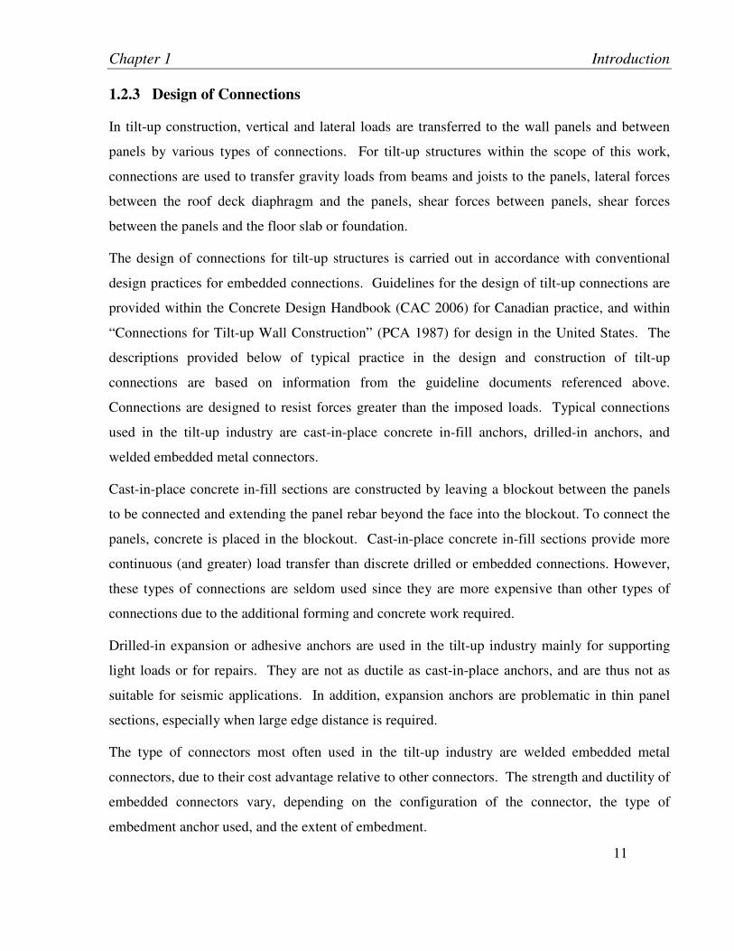
For in-plane load transfer between the wall panels and the roof system, the roof diaphragm
perimeter angle is periodically welded to embedded EM2 or EM3 connectors. Sufficient
connection is provided to accommodate the maximum shear load from the roof diaphragm.
Refer to Figure 1.8 below for an illustration of this connection.
Chapter 1 Introduction
19
Figure 1.8 Deck Connection for In-Plane Forces (Weiler Smith Bowers, 2008)
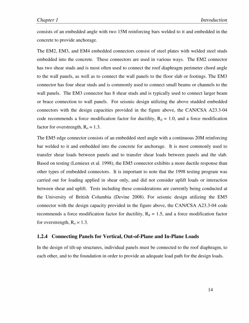
Connections between panels and between panels and the footings or floor slab are typically
designed to resist panel sliding and overturning. The following methodology is presented in the
Concrete Design Handbook (CAC 2006) examples to design panel connections for in-plane
loads:
Figure 1.9 Design Forces for Panel Sliding / Overturning
Width, b
Hei
ght,
h
EM3 to EM5 Connection
EM5 to EM5 Connection
Vroof
Vin-plane walls
Wroof
WPanel
VP/P
VP/S Vertical Reaction
VP/P
WPanel
VHold-down VP/P
WPanel
Wroof Wroof
VP/P
Chapter 1 Introduction
20
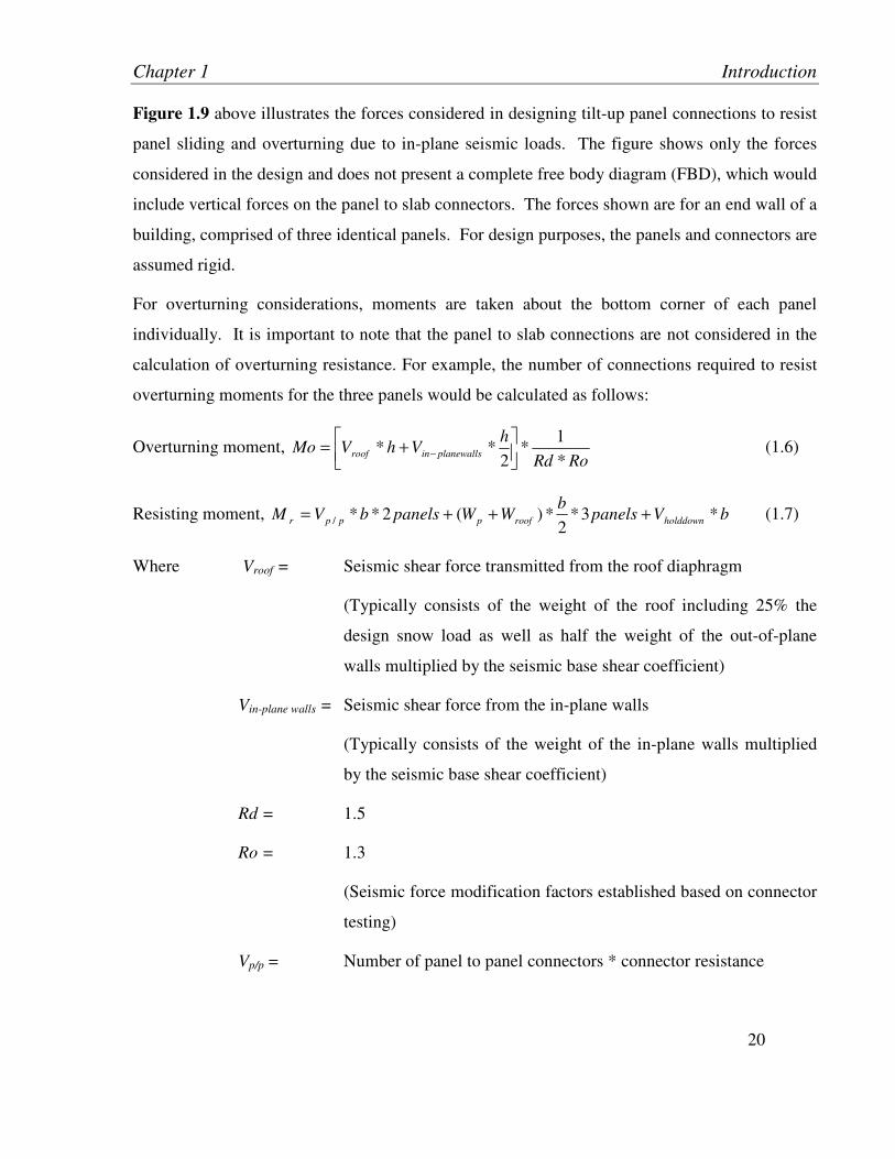
Figure 1.9 above illustrates the forces considered in designing tilt-up panel connections to resist
panel sliding and overturning due to in-plane seismic loads. The figure shows only the forces
considered in the design and does not present a complete free body diagram (FBD), which would
include vertical forces on the panel to slab connectors. The forces shown are for an end wall of a
building, comprised of three identical panels. For design purposes, the panels and connectors are
assumed rigid.
For overturning considerations, moments are taken about the bottom corner of each panel
individually. It is important to note that the panel to slab connections are not considered in the
calculation of overturning resistance. For example, the number of connections required to resist
overturning moments for the three panels would be calculated as follows:
Overturning moment, RoRd
hVhVMo planewallsinroof *
1*
2**
+= −
(1.6)
Resisting moment, bVpanelsb
WWpanelsbVM holddownroofpppr *3*2
*)(2**/ +++=
(1.7)
Where Vroof = Seismic shear force transmitted from the roof diaphragm
(Typically consists of the weight of the roof including 25% the
design snow load as well as half the weight of the out-of-plane
walls multiplied by the seismic base shear coefficient)
Vin-plane walls = Seismic shear force from the in-plane walls
(Typically consists of the weight of the in-plane walls multiplied
by the seismic base shear coefficient)
Rd = 1.5
Ro = 1.3
(Seismic force modification factors established based on connector
testing)
Vp/p = Number of panel to panel connectors * connector resistance
Chapter 1 Introduction
21
(Typically EM5 embedded connectors are used for panel to panel
connections. Connectors are embedded in adjacent panels and
field welded.)
Wp = Weight of panel
Vhold-down = Maximum hold-down weight at corner
(Approximately half the weight of the adjacent connected out-of-
plane panel is assumed to assist in resisting the overturning
moment)
In the calculation of overturning moment in Equation 1.6 above, the seismic force for the in-
plane walls is applied at the centre of gravity. It is important to note that in reality, the
acceleration response of a building in a seismic event is more accurately modeled with a
triangular distribution, which would result in the seismic force being applied at two thirds the
height of the in-plane walls. Based on Equation 1.7 above, sufficient numbers of panel-to-panel
connectors are provided such that the overturning demands due to the applied loads can be
resisted. The following equations illustrate how the panels are designed for sliding
considerations:
[ ]RoRd
VVH planewallsinroofapplied *
1*−+=
(1.8)
µ*)(/ WroofWpVH spresisting ++=
(1.9)
Where Rd = 1.0
Ro = 1.3
(Seismic force modification factors established based on connector
testing)
Vp/s = Number of panel to slab connectors * connector resistance
(Typically EM5 connectors are embedded in the slab and EM3
connectors are embedded in the panel, and the two connectors are
field welded after panel erection.)
Chapter 1 Introduction
22
µ = 0.5 (Coefficient of friction between the panels and footing)
Sufficient numbers of panel to slab connectors are provided such that the applied horizontal
forces can be accommodated.
Using the above design methodology, it is clear that seismic loads less than or equal to the
design loads can be accommodated. However, it is not certain how the system will behave for
seismic loads greater than the design loads. In reality, the connections at the base will undergo
both shear and uplift loads. Also the magnitude of the loads applied on the connectors will
depend on the relative stiffness’ of the panel to panel connectors and the panel to slab connectors
in uplift and shear. It is important to understand the behaviour of a structural system post-yield
in order to ensure that the system can behave in a ductile manner and prevent brittle collapse for
ground motions more severe than the design earthquake.
1.2.5 Design of Roof System
The roof system for tilt-up structures is typically constructed of either wood or steel. Wood
systems consist of plywood decking supported on wood joists, wood beams and steel columns.
Although wood roof systems have been used extensively in the past, steel roof systems are
currently used for most new tilt-up construction. For this reason, this study will focus on steel
roof systems. Steel roof systems consist of steel decking supported on open web steel joists,
steel girders and steel columns. To carry the vertical loads, the steel decking is designed to span
between the open web steel joists, which are supported by either a steel girder or one of the
concrete wall panels. The girders are most often supported on steel columns, though
occasionally they are framed into wall panels due to building layout considerations.
To transfer lateral loads due to earthquakes and wind from the out-of-plane walls and roof into
the in-plane walls, the steel roof decking is designed to act as a diaphragm. The steel decking is
connected to underlying joist members either with pins, screws or by puddle welds. Side laps of
adjacent decking panels are typically fastened by screws, but may also be fastened by button
punching or welding. A steel angle is placed around the perimeter of the deck and fastened to
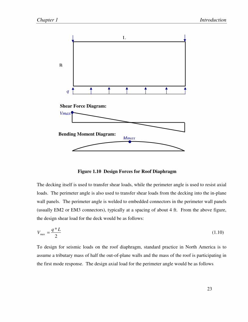
the steel decking by screws, welds, or pins. Figure 1.10 below illustrates the typical free body
diagram used to determine the design forces on the deck and perimeter chord.
Chapter 1 Introduction
23
Figure 1.10 Design Forces for Roof Diaphragm
The decking itself is used to transfer shear loads, while the perimeter angle is used to resist axial
loads. The perimeter angle is also used to transfer shear loads from the decking into the in-plane
wall panels. The perimeter angle is welded to embedded connectors in the perimeter wall panels
(usually EM2 or EM3 connectors), typically at a spacing of about 4 ft. From the above figure,
the design shear load for the deck would be as follows:
2
*max
LqV =
(1.10)
To design for seismic loads on the roof diaphragm, standard practice in North America is to
assume a tributary mass of half the out-of-plane walls and the mass of the roof is participating in
the first mode response. The design axial load for the perimeter angle would be as follows
Shear Force Diagram:
x
Mmax
Vmax
Bending Moment Diagram:
B
L
q
Chapter 1 Introduction
24
B
Lq
B
MCdesign *8
* 2max ==
(1.11)
In Canada, steel deck diaphragms are designed in accordance with a document titled “Design of
Steel Deck Diaphragms – 3rd Edition” (Canadian Sheet Steel Building Institute, 2006). This
document endorses two methods used to determine the shear capacity of deck sections, one
based on the Tri-Services Method (S.B. Barnes and Associates, 1973), and one based on the
Steel Deck Institute (SDI) Method (Steel Deck Institute, 2004). The Tri-Services Method was
developed by S. Barnes and Associates and is based on a series of full-scale tests of steel deck
panels from which empirical equations were developed for strength and stiffness. This method
has limited applicability and is subject to the following restrictions:
• Deck connections to the supporting structure must be welded with 12mm (0.5in)
minimum effective diameter.
• Side-lap connections between deck sheets must be button punched or seam welded.
• Sheet thickness must be at least 0.76mm (0.030 in or 22ga). The maximum thickness is
1.52mm (0.060 in or 16ga).
• Each deck unit must be attached to the framing member by at least two welds.
• Side lap attachments have a maximum spacing of 0.9m (3ft).
• The original tests were based only on horizontal assemblies.
The SDI method was developed by Dr. L.D. Luttrell based on analytical work and tests
conducted at West Virginia University. In this method, the ultimate capacity of the diaphragm is
limited by any one of four failure modes:
• Fastener failure along the outer panel edge.
• Fastener failure around interior panel.
• Failure of the corner fasteners.
• Plate-like shear buckling.

Chapter 1 Introduction
25
Some of the variables selected during design of the deck include the thickness of the deck, the
profile of the deck, the type of fasteners used and the fastening pattern.
The Tri-Services method has often been used in Canada due to its conformity to standard
construction practices and due to its adoption by the Canadian Sheet Steel Building Institute.
However recent testing (Tremblay et. al, 2003) has indicated that welded and button punched
deck connections do not perform favourably when compared to screwed and pinned connections
under applied cyclic loading. This has led to a shift in Canadian practice to the more frequent
use of screwed and pinned connections in seismically active areas, requiring that the design be
carried out using the SDI method. For the purposes of this study, the design of steel deck
diaphragms has been based on using pinned and screwed deck fasteners, and has been carried out
in accordance with the SDI method. Hilti Profis DF Dia software (Hilti Corporation, 2006) was
used to carry out the design of the steel deck diaphragm. Hilti has conducted extensive testing
on various fasteners and has recently proposed a modification factor to apply to SDI calculated
strength and stiffness based on test results (Hilti Corporation, 2008).
For seismic loads, force modification factors are applied depending on the type of fasteners used.
If pins are used to fasten the deck to the underlying members, and screws are used to fasten the
deck sheet side laps, a ductility factor, Rd = 1.5 and an over-strength factor, Ro = 1.3 are
typically used.
1.2.6 U.S. Perspective
The design and construction of tilt-up buildings in the U.S. is done in much the same way as it is
in Canada. The main reference manual used in design is “The Tilt-Up Construction and
Engineering Manual – 6th Edition” (Tilt-up Concrete Association 2005). Currently, the
governing building code used in design of tilt-up structures is the International Building Code
(IBC 2006), which references the concrete design code ACI-318 (2005) issued by the American
Concrete Institute (ACI) for concrete design.
There are no major differences in design provisions between U.S. and Canadian practices for
non-seismic loading. In addition, most construction details are very similar. However, the
consideration of seismic loads in the design of tilt-up structures is carried out slightly differently.

Chapter 1 Introduction
26
The following is a brief summary to highlight the differences in the approach used to calculate
seismic demands in accordance with IBC 2006, in comparison to the NBCC 2005:
The fundamental period is calculated as follows:
43
*02.0 hT = (1.12)
Where:
h = height of the wall panels in feet
Note that Equation (1.12) above, is identical to Equation (1.5) used in Canada when compared
with the same units. Similar to Canadian practice, calculation of the building period does not
account for the flexibility of the roof diaphragm.
The IBC 2006 uses a deterministic approach to obtain the Maximum Credible Earthquake
(MCE) for a given location. The Design Earthquake (DE) is defined as two-thirds of the MCE.
It turns out that for most locations in the US, the MCE is governed by the 2% in 50 year
earthquake which is the same earthquake return period used for the NBCC 2005. Also, since tilt-
up buildings generally fall within the short period cut-off defined in the NBCC 2005, the
earthquake demands prescribed by the NBCC 2005 are multiplied by 2/3 to obtain the design
base shear. As such, the earthquake demands based on US and Canadian codes are equivalent.
Force modification factors (R values) are treated slightly differently in US codes than in the
NBCC 2005. In US codes, there is no distinction between factors accounting for overstrength
and factors accounting for ductility (Ro and Rd in the NBCC 2005). A single R value is
prescribed, depending on the lateral load resisting system. Within the IBC 2006, tilt-up
structures fall in the category of load bearing ordinary precast shear walls, for which an R value
of 3.0 is prescribed.
1.2.7 Discussion of Current Design Methods
The methods described above for seismic design of tilt-up structures constitute a force-based
approach. The structural system is designed to accommodate seismic forces calculated in
Chapter 1 Introduction
27
accordance with the building code. One major drawback of the approach described above is that
there is little consideration for capacity design principles commonly incorporated into other
structural systems currently in use. In essence, there is no clear, stable failure mechanism for the
system, since the standard connectors used do not have sufficient ductility in the direction in
which they are loaded to allow a stable mechanism to form.
Another problem with the current design approach is that the code calculated fundamental period
of the building currently used to establish seismic demands does not account for the flexibility of
the steel roof deck, and thus does not accurately predict the fundamental period for a typical
single story tilt-up structure.
1.3 Previous Research
1.3.1 Roof Diaphragm
A reasonable assessment of the strength and stiffness of the roof deck diaphragm is important in
this study in order to ensure that:
• The diaphragm for the archetypical building is appropriately designed
• The stiffness of the diaphragm is reasonably estimated and incorporated into the analysis
model
• The strength of the deck is appropriately estimated when compared with demands from
the analysis.
There has been considerable research on the behaviour of corrugated cold-formed steel deck
diaphragms and many tests have been conducted, though most have been performed under
monotonically increasing load (Nilson, 1960; Easley and McFarland, 1969; Luttrell and Ellifritt,
1970; Easly, 1977; Steel Deck Institute (SDI), 1981; Klingler, 1996; Lemay and Beaulieu, 1986).
Seismic loading is inherently cyclical, and therefore the results of these tests may not be
applicable for this study. More recently, several tests have been conducted incorporating cyclical
loading. In one study (Essa, Tremblay and Rogers, 2003), 18 large scale tests were carried out
on diaphragm assemblies made with 22ga (0.76mm) and 20ga (0.91mm) thick metal deck sheets
using various types of fasteners in various configurations. The tests were performed using a

Chapter 1 Introduction
28
cantilever type configuration for the test setup, with the steel deck diaphragm in a horizontal
plane. Both cyclic and monotonic testing was conducted. Figure 1.11 below (Essa, Tremblay
and Rogers 2003) illustrates the test setup used.
Figure 1.11 Schematic of Test Setup
Nine different configurations of fasteners and deck thicknesses were included in the program.
Two specimens were constructed for each configuration; one was tested with monotonic loading
and one with cyclic loading. The loading protocols used are illustrated in Figure 1.12 below
(Essa, Tremblay and Rogers 2003).
Figure 1.12 Monotonic and Quasistatic Cyclic Loading Protocols

Chapter 1 Introduction
29
In the above figure, D1 and D2 are determined from the monotonic testing to be used in the
cyclic testing. D1 is the displacement assuming the specimen remains elastic based on the secant
stiffness up to the peak load. D2 is the actual displacement at the peak load.
The fastening configurations and corresponding deck thicknesses tested are shown in the table
below [Essa, Tremblay and Rogers 2003]. Of particular interest are Test No.’s 4, 7, 17 and 18,
which incorporate B-Deck nestable deck profile with nailed (Hilti) deck to frame fasteners and
screwed side lap fasteners, since this configuration was adopted for this study. These have been
outlined in Table 1.1 below.
Table 1.1 Deck Test Specimens – Fastening Configurations (Essa, Tremblay and Rogers
2003)
The table below provides the results for the monotonic testing [Essa, Tremblay and Rogers
2003]. The results of interest are outlined.
Table 1.2 Results from Monotonic Testing (Essa, Tremblay and Rogers, 2003)
Chapter 1 Introduction
30
In the above table, the SDI* values of strength and stiffness were based on prior monotonic
testing [Rogers and Tremblay, 2003]. It is believed there is an error in the table in the title of
the third column from the left. It seems the intent of the authors was to compare strength results
from testing to SDI calculated strengths, not SDI* calculated strengths. The results for the cyclic
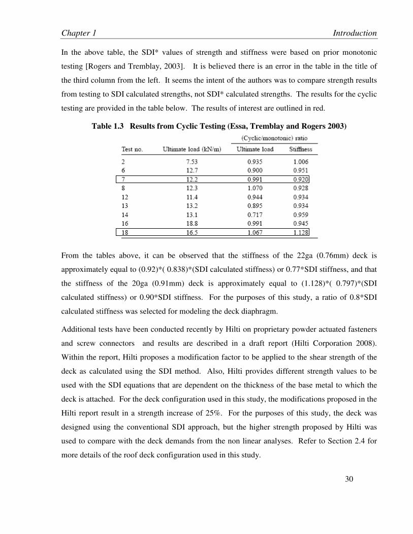
testing are provided in the table below. The results of interest are outlined in red.
Table 1.3 Results from Cyclic Testing (Essa, Tremblay and Rogers 2003)
From the tables above, it can be observed that the stiffness of the 22ga (0.76mm) deck is
approximately equal to (0.92)*( 0.838)*(SDI calculated stiffness) or 0.77*SDI stiffness, and that
the stiffness of the 20ga (0.91mm) deck is approximately equal to (1.128)*( 0.797)*(SDI
calculated stiffness) or 0.90*SDI stiffness. For the purposes of this study, a ratio of 0.8*SDI
calculated stiffness was selected for modeling the deck diaphragm.
Additional tests have been conducted recently by Hilti on proprietary powder actuated fasteners
and screw connectors and results are described in a draft report (Hilti Corporation 2008).
Within the report, Hilti proposes a modification factor to be applied to the shear strength of the
deck as calculated using the SDI method. Also, Hilti provides different strength values to be
used with the SDI equations that are dependent on the thickness of the base metal to which the
deck is attached. For the deck configuration used in this study, the modifications proposed in the
Hilti report result in a strength increase of 25%. For the purposes of this study, the deck was
designed using the conventional SDI approach, but the higher strength proposed by Hilti was
used to compare with the deck demands from the non linear analyses. Refer to Section 2.4 for
more details of the roof deck configuration used in this study.
Chapter 1 Introduction
31
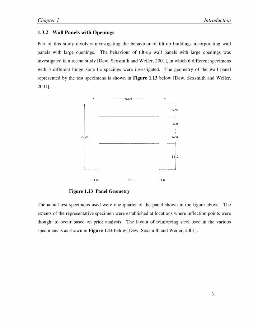
1.3.2 Wall Panels with Openings
Part of this study involves investigating the behaviour of tilt-up buildings incorporating wall
panels with large openings. The behaviour of tilt-up wall panels with large openings was
investigated in a recent study [Dew, Sexsmith and Weiler, 2001], in which 6 different specimens
with 3 different hinge zone tie spacings were investigated. The geometry of the wall panel
represented by the test specimens is shown in Figure 1.13 below [Dew, Sexsmith and Weiler,
2001].
Figure 1.13 Panel Geometry
The actual test specimens used were one quarter of the panel shown in the figure above. The
extents of the representative specimen were established at locations where inflection points were
thought to occur based on prior analysis. The layout of reinforcing steel used in the various
specimens is as shown in Figure 1.14 below [Dew, Sexsmith and Weiler, 2001].
Chapter 1 Introduction
32
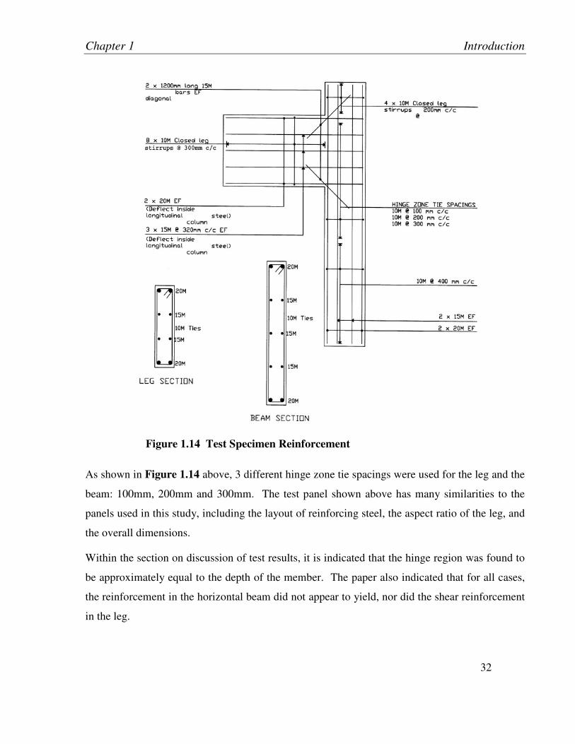
Figure 1.14 Test Specimen Reinforcement
As shown in Figure 1.14 above, 3 different hinge zone tie spacings were used for the leg and the
beam: 100mm, 200mm and 300mm. The test panel shown above has many similarities to the
panels used in this study, including the layout of reinforcing steel, the aspect ratio of the leg, and
the overall dimensions.
Within the section on discussion of test results, it is indicated that the hinge region was found to
be approximately equal to the depth of the member. The paper also indicated that for all cases,
the reinforcement in the horizontal beam did not appear to yield, nor did the shear reinforcement
in the leg.

Chapter 1 Introduction
33
It is observed in the paper that the specimens with a tie spacing of either 100mm or 200mm
maintained the design flexural strength of the specimen even on the third cycle of their load
sequence, while the specimens with a tie spacing of 300mm did not. The design flexural
strength was defined using stress block methods assuming an ultimate concrete stain of 0.0035.
Displacement ductility was determined for the various tests. Displacement ductility is defined as
follows:
∆
∆=
yield
ultDuctility
(1.13)
Where: ∆ult = Ultimate displacement
∆yield =Yield displacement
In this paper, the yield displacement was assumed to occur when a bending moment equal to the
design flexural strength was applied to the specimen, while the ultimate displacement was
assumed to occur when the specimen could no longer maintain the design flexural strength.
The calculated ductility of the specimens was used to estimate an appropriate force reduction
factor for the specimens. Since the fundamental period of the tilt-up panels was expected to be
in the order of 0.2 seconds, which is significantly less than the period at the peak spectral
acceleration in the design spectrum, it was assumed that the equal energy principle could be
applied to determine an appropriate force reduction factor for the specimens. The equal energy
principle states the force reduction factor is calculated as follows:
( ))1*2 −= DuctilityR (1.14)
A force reduction value (Rd*Ro) of 2.0 is commonly used for the design of tilt-up frame panel
legs. Based on the test results, this paper indicated that a force reduction value of 2.0 is
reasonable for the specimens tested if a maximum tie spacing of 200mm is used. As such, these
values were incorporated in this study.
1.3.3 Building System
There has been some previous work carried out to investigate the behaviour of the overall
building system for tilt-up structures subjected to earthquakes. One recent study (Adebar, Guan

Chapter 1 Introduction
34
and Elwood, 2004) investigated the amplification of inelastic drifts in concrete tilt-up frames due
to steel deck roof diaphragms designed to remain elastic during the design earthquake. The
above study proposed a simplified approach to estimate the inelastic drifts in concrete tilt-up
panels with openings for walls subjected to in-plane seismic loading, which is described in the
following equation:
)1(*)(we
wy
dwiV
VTS −=∆ (1.15)
Where: ∆wi = Inelastic Wall Displacement
Sd(T) = Spectral displacement at the centre of the roof at the fundamental
period of the building
Vwy = Wall strength
Vwe = Maximum elastic demand for the wall
This approach was validated with results from nonlinear analyses of simplified models of
various configurations for tilt-up buildings incorporating panels with openings.
Another study (Hawkins, Wood and Fonseca, 1994) investigated the possibility of using a
detailed analytical model to reproduce the measured response of an instrumented tilt-up
warehouse located in Hollister, California, subjected to the 1989 Loma Prieta Earthquake. The
study reported good correspondence between results from the analysis and the measured
response, and was helpful in developing the analytical model used for the current work.
The American Society of Civil Engineers (ASCE) Standard 41-06, titled “Seismic Rehabilitation
Standard” provides guidelines for estimating both building period and the out-of-plane seismic
load distribution on the roof diaphragm for single story structures with flexible diaphragms. It
appears that the guidelines provided in the above standard are not incorporated either in
American or Canadian practice for the design of tilt-up structures. The ASCE 41-06
approximations for building period and out-of-plane loading on the roof diaphragm will be
compared with the analysis results from this study within Section 3.2.

Chapter 1 Introduction
35
1.4 Research Aims
1.4.1 Evaluate Previous Research on Building System
Within this study, a simplified approach previously proposed (Adebar, Guan and Elwood, 2004)
to estimate the inelastic drifts in concrete tilt-up panels with openings is compared with results
from non-linear analyses using a detailed finite element model. Other conclusions from the
above study, including the effect of yielding in-plane walls on the roof displacement are also
investigated with a detailed model.
In addition, results from the analyses are compared with the following items:
• Determination of building period based on NBCC 2005 and ASCE 41-06, and
• Seismic demands on the roof diaphragm due to out-of-plane response of wall panels
based on ASCE 41-06 and common North American practice.
1.4.2 Investigate Alternatives for Capacity Design
The concept of capacity design is considered in the seismic design of most modern structures.
Capacity design essentially requires that there be a clearly identifiable, ductile mechanism in the
lateral load resisting system of a building, thus providing occupants with ample warning prior to
failure. Current methods for the design of tilt-up structures do not incorporate the principles of
capacity design. Panels are connected together to resist code-prescribed seismic forces.
Connections are designed with R values selected based on results from testing of individual
connectors. The roof diaphragm is designed with an R value selected based on results from
testing of steel deck diaphragms. It is difficult to assess how tilt-up buildings designed to current
practice would behave in an earthquake, since the interactions between the various components
are so complex. One objective of this study is to investigate alternatives for failure mechanisms
that could be incorporated into the seismic design of tilt-up structures to meet the intent of
capacity design. Sliding, rocking and frame mechanisms are considered for tilt-up panels. Given
that this study focuses on the behaviour of the wall panels, a failure mechanism resulting from
yielding of the roof deck diaphragm is not considered.
Chapter 1 Introduction
36
1.4.3 Quantify Building Performance for Selected Mechanisms
R-values for buildings have traditionally been selected based on results from component testing,
historical performance of building systems in past earthquakes, and judgement. It is more
difficult to select R-values for new building systems without historical data on performance in
major earthquakes. One methodology to assess R-values for new building systems has been
recently proposed by the Applied Technology Council (ATC) in the U.S. and is described in a
document titled “Quantification of Building Seismic Performance Factors - ATC-63 Project
Report – 90% Draft” (ATC, 2008). The intent of the ATC-63 Methodology is to provide a
rational approach to quantify building system performance and select R-values. In this study,
aspects of the ATC-63 Methodology will be used as a guideline to assist in selecting R-values
for building designs incorporating the various failure mechanisms considered.
1.4.4 Thesis Organization
To address the objectives outlined above, Chapter 2 will describe the assessment methodology
used to quantify building performance. Chapter 3 will describe an investigation of the various
mechanism alternatives considered for tilt-up structures, including results from analyses, an
evaluation of how the analysis data compares with previous research, and proposed connection
details. Chapter 4 will describe the results from analyses conducted to quantify building
performance. Chapter 5 will provide conclusions and recommendations with regards to this
study.
37
2 ASSESSMENT METHODOLOGY
2.1 General
The assessment methodology used in this study to quantify tilt-up building performance for
selected mechanisms is based on concepts from the ATC-63 Methodology (ATC 2008), which
was developed to quantify building system performance and response parameters for use in
seismic design. The assessment methodology used in this study does not follow all of the steps
of the ATC-63 Methodology.
The stated objective of the ATC-63 Methodology is to provide a “rational basis for establishing
global seismic performance factors (SPF’s), including the response modification coefficient (R
Factor), of new seismic force-resisting systems proposed for construction and inclusion in model
building codes and resource documents. It also provides a more rational basis for re-evaluation
of the SPF’s of existing seismic force-resisting systems.”
R factors are used in both Canadian and U.S. building codes to estimate demands for seismic
load resisting systems that are designed using linear methods but are expected to respond beyond
the linear range for the design earthquake. In the 2005 National Building Code of Canada, R
factors are separated into an overstrength term, Ro and a ductility term, Rd, and the two terms are
multiplied together to determine the overall reduction to elastic demands. R factors have a
tremendous effect on the design requirements for a given building. For example, for the design
of a tilt-up building to be located in Vancouver B.C., typical values for Ro and Rd would be 1.3
and 1.5 respectively for the majority of the components of the seismic load resisting system.
This means a reduction in the forces determined from linear elastic analysis by a factor of
(1.3)*(1.5) = 2.0.
Traditionally, R factors have been derived based on judgement, observations of the performance
of existing structures in previous earthquakes, and observations from component testing.
However, many recently defined seismic force resisting systems have not been exposed to
significant earthquakes, and their abilities to meet the design requirements are uncertain. In
Chapter 2 Assessment Methodology
38
addition, assessment of R factors by the traditional approach likely leads to considerable
variability in seismic performance between the various seismic force resisting systems. The
intent of the ATC-63 Methodology is to ensure that different seismic force resisting systems
have a similarly low probability of collapse for the design earthquake.
The ATC-63 Methodology is based on applicable design criteria and requirements of the ASCE
7-05 “Minimum Design Loads for Buildings and Other Structures” provisions. However for the
purposes of this study, the ATC-63 Methodology is adapted to structures designed in accordance
with the 2005 NBCC provisions.
The ATC-63 Methodology involves the following process:
• Representative structures are identified to capture the various types of applications for the
seismic force resisting system in practice. Refer to Section 2.4 for the representative
structures used in this study.
• The representative structures are designed in a manner consistent with how they would
be designed in practice, with trial R values. Refer to Section 2.4 for more detail on the
design of the buildings investigated in this study.
• Analytical models of the representative structures are then developed, incorporating all
non-linear component behaviour required to simulate collapse. Refer to Section 2.5 for
general aspects of the non linear modeling.
• Non-linear Incremental Dynamic Analysis (IDA), (Vamvatsikos and Cornell, 2002) is
carried out for each model for a suite of earthquake records. Refer to Section 2.5 for a
description of the IDA procedure.
• The earthquake intensity required to cause collapse is determined for each earthquake
record, and collapse statistics are generated (Refer to Section 2.6).
• If the probability of collapse at the design earthquake intensity is sufficiently low, the R
factor used to design the structure is deemed appropriate. If not, the R-factor is modified,
the strength of the seismic force resisting system is adjusted accordingly and the process
is repeated until an appropriate R factor is determined.

Chapter 2 Assessment Methodology
39
The sections below describe the ATC-63 Methodology in more detail.
2.2 Seismic Performance Factors
Within the ATC-63 Methodology, Seismic Performance Factors include the response
modification coefficient related to ductility (R factor in the ASCE7-05 and Rd in the 2005
NBCC) and the system over-strength factor (Ωo in the ASCE7-05 and Ro in the 2005 NBCC).
Hereafter within this report these two factors will be referred to as Rd and Ro. ATC-63 can also
be used to evaluate the displacement amplification factor, Cd. However the overall conclusion
from the report is that, Cd = R. Figure 2.1 and Figure 2.2 below illustrates conceptually how
SPF’s are considered within the ATC-63 Methodology, and how they are incorporated in both
Canadian and U.S. practice.
Figure 2.1 Seismic Performance Factors - Canadian Practice
Sp
ectr
al
Acc
eler
ati
on
(g
)
Spectral Displacement
Cs
Smax
SMT
Ro
SDMT
Design Earthquake
RD
Legend:
RD = Force reduction factor based on ductility
Ro = Force reduction factor based on over-strength
SDMT = Drift due to design earthquake
SDCT = Drift due to collapse level earthquake
ŜCT = Spectral acc. at collapse level earthquake
SMT = Spectral acceleration at design level earthquake
CS = Spectral acceleration used for design (=SMT/RdRo)
CMR = Collapse Margin Ratio
( = ŜCT /SMT)
CMR ŜCT Collapse Level
Earthquake
SDCT SDMT
RdRO

Chapter 2 Assessment Methodology
40
Figure 2.2 Seismic Performance Factors - US Practice
Within Figure 2.1 and Figure 2.2 above, CMR refers to the collapse margin ratio, which is a
ratio of the median spectral acceleration observed at collapse of the structure from the analysis
divided by the design spectral acceleration. A minimum CMR value is required in order to
ensure a sufficiently low probability of collapse at the design earthquake. This will be discussed
further in Section 2.6 on Collapse Fragility.
2.3 Seismic Hazard
2.3.1 Ground Motion Record Sets
The earthquake records considered in the ATC-63 Methodology consist of twenty-two ground
motion record pairs from sites located more 10km from fault rupture. Within the ATC-63
document, they are referred to as “Far-Field” records. All of the records used in the
methodology are from large magnitude events in the PEER NGA database, varying from a

Chapter 2 Assessment Methodology
41
Magnitude 6.5 to 7.6 on the Richter scale. The ground motion records selected represent various
site conditions and source mechanisms. A maximum of two record pairs are used from each
earthquake, so as to avoid event bias. A sufficient number of records are considered to allow
statistical evaluation of record-to-record variability and collapse fragility. Table below provides
a summary of the ground motion records used within this study.
Table 2.1 Summary of Ground Motion Records (ATC-63, 2008)
M Year Name Name Owner Component 1 Component 2PGAmax
(g)
PGVmax
(cm/s)
1 6.7 1994 Northridge Beverly Hills - Mulhol USC NORTHR/MUL009 NORTHR/MUL279 0.52 63
2 6.7 1994 Northridge Canyon County - WLC USC NORTHR/LOS000 NORTHR/LOS270 0.48 45
3 7.1 1999 Duzce, Turkey Bolu ERD DUZCE/BOL000 DUZCE/BOL090 0.82 62
4 7.1 1999 Hector Mine Hector SCSN HECTOR/HEC000 HECTOR/HEC090 0.34 42
5 6.5 1979 Imperial Valley Delta UNAMUCSD IMPVALL/H-DLT262 IMPVALL/H-DLT362 0.35 33
6 6.5 1979 Imperial Valley El Centro Array #11 USGS IMPVALL/H-E11140 IMPVALL/H-E11230 0.38 42
7 6.9 1995 Kobe, Japan Nishi-Akashi CUE KOBE/NIS000 KOBE/NIS090 0.51 37
8 6.9 1995 Kobe, Japan Shin-Osaka CUE KOBE/SHI000 KOBE/SHI090 0.24 38
9 7.5 1999 Kocaeli, Turkey Duzce ERD KOCAELI/DZC180 KOCAELI/DZC270 0.36 59
10 7.5 1999 Kocaeli, Turkey Arcelik KOERI KOCAELI/ARC000 KOCAELI/ARC090 0.22 40
11 7.3 1992 Landers Yermo Fire Station CDMG LANDERS/YER270 LANDERS/YER360 0.24 52
12 7.3 1992 Landers Coolwater SCE LANDERS/CLW-LN LANDERS/CLW-TR 0.42 42
13 6.9 1989 Loma Prieta Capitola CDMG LOMAP/CAP000 LOMAP/CAP090 0.53 35
14 6.9 1989 Loma Prieta Gilroy Array #3 CDMG LOMAP/G03000 LOMAP/G03090 0.56 45
15 7.4 1990 Manjil, Iran Abbar BHRC MANJIL/ABBAR-L MANJIL/ABBAR-T 0.51 54
16 6.5 1987 Superstition Hills El Centro Imp. Co. CDMG SUPERST/B-ICC000 SUPERST/B-ICC090 0.36 46
17 6.5 1987 Superstition Hills Poe Road (temp) USGS SUPERST/B-POE270 SUPERST/B-POE360 0.45 36
18 7.0 1992 Cape Mendocino Rio Dell Overpass CDMG CAPEMEND/RIO270 CAPEMEND/RIO360 0.55 44
19 7.6 1999 Chi-Chi, Taiwan CHY101 CWB CHICHI/CHY101-E CHICHI/CHY101-N 0.44 115
20 7.6 1999 Chi-Chi, Taiwan TCU045 CWB CHICHI/TCU045-E CHICHI/TCU045-N 0.51 39
21 6.6 1971 San Fernando LA - Hollywood Stor CDMG SFERN/PEL090 SFERN/PEL180 0.21 19
22 6.5 1976 Fiuli, Italy Tolmezzo - FRIULI/A-TMZ000 FRIULI/A-TMZ270 0.35 31
ID
No.
Earthquake Recording StationNGA Record Information (File Names -
Horizontal Records)
Recorded
Motions

Chapter 2 Assessment Methodology
42
2.3.2 Ground Motion Record Scaling
To carry out incremental dynamic analysis, further described in Section 2.5.4, earthquake
records are scaled up until the collapse capacity of the structure is determined. In the ATC-63
Methodology the earthquake record scaling is done in two steps. In the first step, the records are
normalized by their peak ground velocities in an effort to remove variability between records due
to inherent differences in event magnitude, distance to source, source type and site conditions,
without removing the record-to-record variability required for IDA. In the second step, the
records are collectively scaled so as to determine the collapse capacity for the structure and IDA
plots are generated.
The scaling method recommended by ATC-63, specifically the first step in the scaling process, is
limiting in terms of statistical analysis of the data. All of the IDA graphs are plotted in terms of
spectral acceleration at the first mode of the structure vs. drift. When records are normalized in
terms of their peak ground velocities, the “normalized” records result in very different spectral
accelerations at a given period. This means that when IDA results are plotted for a given scaling
factor, data points from all of the records will have very different spectral acceleration and drift
values. As such it is impossible to determine a median IDA curve from the data if the records
are scaled in this manner. For the purposes of the ATC-63 Methodology, a median IDA curve is
not required since failure of the structure is typically modelled explicitly, and the methodology
only requires the spectral acceleration at median collapse to be determined. Within this study
however, it is necessary to obtain the median IDA curve, since collapse of the structure is not
explicitly modelled but must be determined by comparing results from analyses with capacity
limits. For this reason, the scaling method recommended by ATC-63 was not used.
In order to enable extraction of a median IDA curve from the data, it was elected to normalize
the records by the spectral acceleration at the first period of the structure for the purposes of this
study. This means that for each of the 22 record pairs applied to the model, each of the records
applied in the direction of the first mode of the structure would result in the same spectral
acceleration. This method of scaling provides some consistency in the plotted data and allows
extraction of a meaningful median IDA curve. During the course of the study it was determined
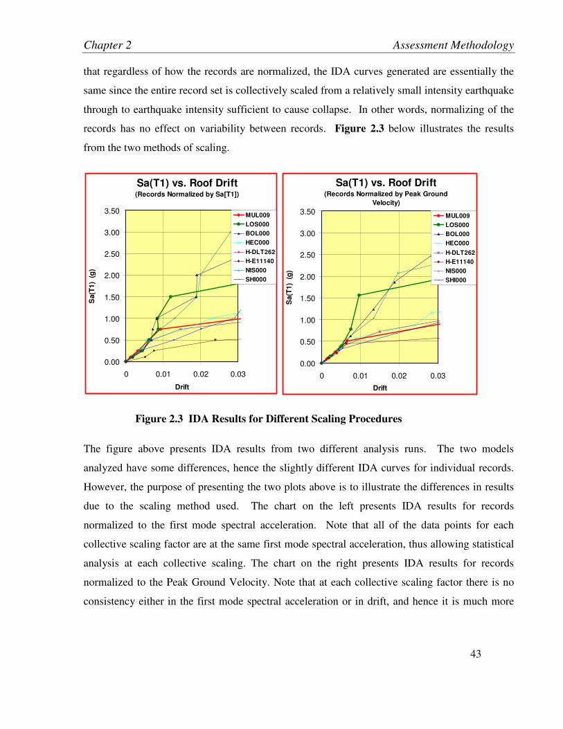
Chapter 2 Assessment Methodology
43
that regardless of how the records are normalized, the IDA curves generated are essentially the
same since the entire record set is collectively scaled from a relatively small intensity earthquake
through to earthquake intensity sufficient to cause collapse. In other words, normalizing of the
records has no effect on variability between records. Figure 2.3 below illustrates the results
from the two methods of scaling.
Sa(T1) vs. Roof Drift(Records Normalized by Sa[T1])
0.00
0.50
1.00
1.50
2.00
2.50
3.00
3.50
0 0.01 0.02 0.03
Drift
Sa(T
1)
(g
)
MUL009
LOS000
BOL000
HEC000
H-DLT262
H-E11140
NIS000
SHI000
Sa(T1) vs. Roof Drift(Records Normalized by Peak Ground
Velocity)
0.00
0.50
1.00
1.50
2.00
2.50
3.00
3.50
0 0.01 0.02 0.03
Drift
Sa(T
1)
(g
)
MUL009
LOS000
BOL000
HEC000
H-DLT262
H-E11140
NIS000
SHI000
Figure 2.3 IDA Results for Different Scaling Procedures
The figure above presents IDA results from two different analysis runs. The two models
analyzed have some differences, hence the slightly different IDA curves for individual records.
However, the purpose of presenting the two plots above is to illustrate the differences in results
due to the scaling method used. The chart on the left presents IDA results for records
normalized to the first mode spectral acceleration. Note that all of the data points for each
collective scaling factor are at the same first mode spectral acceleration, thus allowing statistical
analysis at each collective scaling. The chart on the right presents IDA results for records
normalized to the Peak Ground Velocity. Note that at each collective scaling factor there is no
consistency either in the first mode spectral acceleration or in drift, and hence it is much more
Chapter 2 Assessment Methodology
44
difficult to carry out statistical analysis at each collective scaling factor and obtain a meaningful
median IDA response curve.
2.4 Archetypical Systems
Seismic force resistance systems are often used in more than one type of building and can be
used in a broad range of applications. In order to evaluate the collapse performance of a seismic
force resisting system, the various applications of that system must be characterized into a set of
typical structures that can then be studied. The ATC-63 Methodology refers to these typical
structures as Archetypical systems. For the purposes of this study, a survey was conducted
amongst tilt-up designers in both the U.S. and Canada to assess the most common characteristics
of single story tilt-up structures with steel deck diaphragms. The results of the survey are
summarized in the table below.

Chapter 2 Assessment Methodology
45
Table 2.2 Industry Survey Results – Typical Single Story Tilt-up Building Attributes
Typical Roof Diaphragm Attributes:
1 Percentage of steel, wood, and hybrid deck systems:
Steel: 75% Wood: 0% Hybrid: 25% (US)
Steel: 99% Wood: 0% Hybrid: 0% (Canada)
2 Percentage of connections used for deck:
Puddle Welds: 80% Mech fasteners: 20% (US)
Puddle Welds: 25% Mech fasteners: 75% (Canada)
3 Deck profile:1.5" wide rib type B deck
painted most common
4 Deck thicknesses used: 16ga, 18ga, 20ga, 22ga
5 Range of deck thicknesses: 2
6Percentage of out-of-plane wall mass
apportioned to the roof diaphragm.50%
Typical Building Attributes:
1 Height of Tilt-up Walls (pin to pin) 30 ft
2Ratio of Height to Thickness of Tilt-up
walls50
3 Structural thickness (excludes reveal) 7.25 in
4 Weight of Panels 60000 lb
5 Plan dimensions of buildings 100x200 ft x ft
6Span between LFRS supporting
diaphragm
Maximum of 2 x width in high
seismic zones
7 Joist Span 50 ft
8 Joist Spacing 6.25 ft
9 Joist depth 42 in
10 Girder Span 37.5 ft
11 Girder depth 30 in
12Roof Dead Weight including joists,
diaphragm, insulation, ballast (psf)20 lb/ft
2
Embedded Connectors
1 Number of Connectors between panels As required
2Number of Panel to Floor Slab
Connections (per panel)4 feet o.c.
3Number of Panel to Footing
Connections (per panel)0
4Number of Floor Slab to Footing
Connections (per panel)As required
5Spacing of Diaphragm chord angle to
wall panel connectionsJoist spacing or 4 ft

Chapter 2 Assessment Methodology
46
The survey results reported above indicate only the most common value for each building
attribute. The actual survey results contain a range of the most likely characteristics for each
attribute. Based on the survey results above, two archetypical building systems were established
in order to incorporate the most common building characteristics that would have the greatest
impact on the seismic force resisting system. It is important to note that not all building sizes
have been considered in this study, as would be required to fully conform to the ATC-63
Methodology. Also, in the ATC-63 Methodology, the R factor is evaluated based on the
combined results of all the archetypes, while within this study, R factors are evaluated for each
archetype individually. This is done because the two archetypes considered have very different
mechanisms. One building archetype incorporates solid wall panels, while the other incorporates
panels with openings. Each of the archetypical buildings were designed using conventional
procedures based on the 2005 NBCC for a location in Vancouver, BC with foundation Site Class
D. The following characteristics are common for both building archetypes:
• The building plan dimensions are 30.48m (100ft) x 60.96m (200ft).
• The roof deck system is 38mm (1.5”) deep, Type B steel decking. 18ga and 20ga
decking is used.
• Deck fasteners consist of No. 12 screws at deck sheet side laps and end laps and Hilti
pins to connect deck sheets to underlying steel members. Hilti Profis software (Hilti
2008) was used to design the deck fasteners in accordance with Steel Deck Institute
requirements and Canadian safety factors.
• The roof deck perimeter angle was designed in accordance with SDI requirements. The
perimeter angle is welded to embedded connectors in wall panels at 4ft centre to centre
spacing.
• Joists are 1050mm (3’-6”) deep with L/L chord members. A catalogue produced by
Omega was used to design joists and determine chord properties.
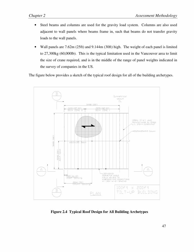
Chapter 2 Assessment Methodology
47
• Steel beams and columns are used for the gravity load system. Columns are also used
adjacent to wall panels where beams frame in, such that beams do not transfer gravity
loads to the wall panels.
• Wall panels are 7.62m (25ft) and 9.144m (30ft) high. The weight of each panel is limited
to 27,300kg (60,000lb). This is the typical limitation used in the Vancouver area to limit
the size of crane required, and is in the middle of the range of panel weights indicated in
the survey of companies in the US.
The figure below provides a sketch of the typical roof design for all of the building archetypes.
Figure 2.4 Typical Roof Design for All Building Archetypes

Chapter 2 Assessment Methodology
48
The design of the steel deck diaphragm was separated into zones based on required resistance.
Zones 1 and 2 were used for the design of the roof and are called up in the above sketch. The
diaphragm zones are illustrated in Figure 2.5 below.
Figure 2.5 Roof Diaphragm Zones
2.4.1 Archetypical System 1: Solid Wall Panels
Archetypical System 1 is based on a building with solid tilt-up wall panels that are 184mm
(7.25”) thick. This is a popular thickness since it is the actual width of a 2”x8” piece of lumber,
allowing for easy forming of the panels, and also because it provides for a reasonable height to
width ratio of approximately 50 for a 9.144m (30ft) high panel. The building layout for the
archetype is much simpler than a “real” building layout, and does not include features such as re-
entrant corners, loading bays, office floors, etc. This was done in order to investigate the overall
seismic response of the building system. The design notes for this archetype building are
included in Appendix A. Figure 2.6 below illustrates details for concrete outline, reinforcement
and connections.
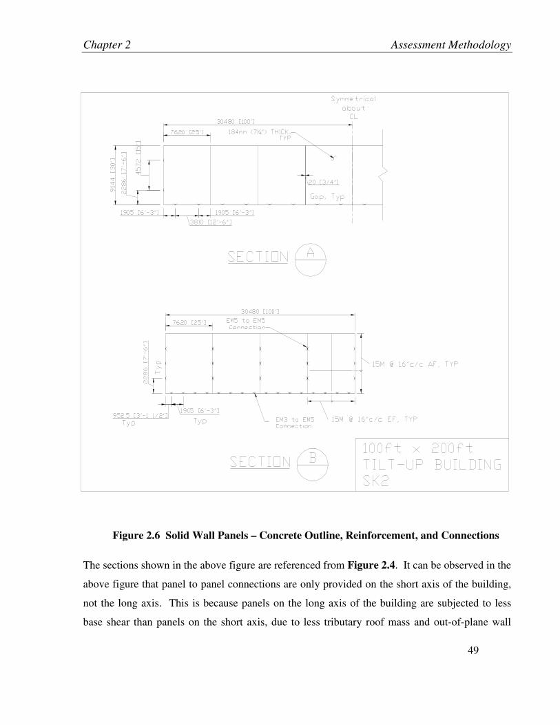
Chapter 2 Assessment Methodology
49
Figure 2.6 Solid Wall Panels – Concrete Outline, Reinforcement, and Connections
The sections shown in the above figure are referenced from Figure 2.4. It can be observed in the
above figure that panel to panel connections are only provided on the short axis of the building,
not the long axis. This is because panels on the long axis of the building are subjected to less
base shear than panels on the short axis, due to less tributary roof mass and out-of-plane wall

Chapter 2 Assessment Methodology
50
mass acting per unit length. Calculations to determine the number of connectors are included in
the design notes for this archetype building (Appendix B).
2.4.2 Archetypical System 2: Wall Panels with Openings
Archetypical System 2 is based on a building with tilt-up wall panels with openings 5.62m (18’-
5”) wide x 3.625m (11’-11”) high. The panels are 240mm (9.5”) thick as required to
accommodate the out-of-plane loading. The dimensions of the panels openings and legs were
selected such that the aspect ratio of the panel legs was the same as that used for recent
experimental testing of panel legs (Dew et. al., 2001). This was done to ensure that the
experimental results could be used to calibrate the numerical model.
The openings in the panels are incorporated since they are often required for tilt-up buildings in
practice to allow for loading docks, or for the front side of commercial or retail buildings. The
design notes for this archetype building are included in Appendix B. Figure 2.7 below illustrates
details for concrete outline, reinforcement and connections (the sections shown are referenced
from Figure 2.4.)
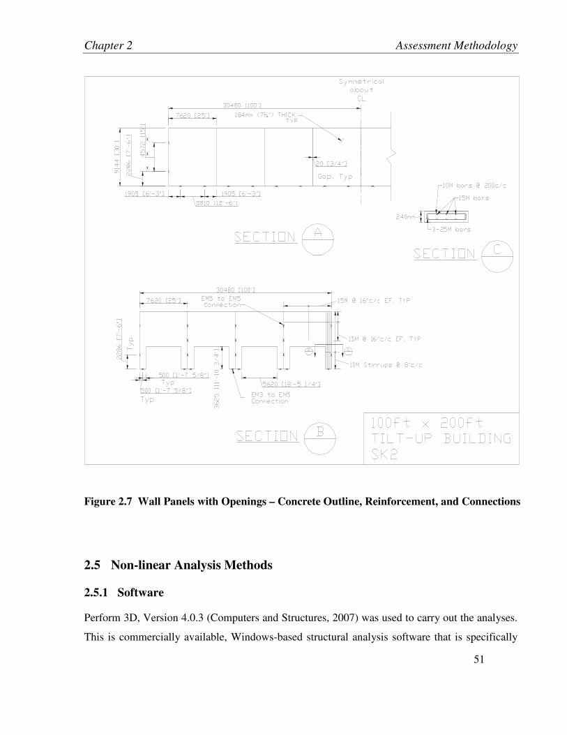
Chapter 2 Assessment Methodology
51
2.5 Non-linear Analysis Methods
2.5.1 Software
Perform 3D, Version 4.0.3 (Computers and Structures, 2007) was used to carry out the analyses.
This is commercially available, Windows-based structural analysis software that is specifically
Figure 2.7 Wall Panels with Openings – Concrete Outline, Reinforcement, and Connections

Chapter 2 Assessment Methodology
52
designed for non-linear time history analyses and performance assessment for 3D structures.
The software contains an element library sufficiently comprehensive to adequately model most
conventional structures and components and provides a graphical interface for pre and post
processing. In addition, it allows the user to set up multiple earthquake analysis runs in
succession and provides the option to apply three different earthquake records on three different
axes simultaneously. The software uses an event-to-event solution strategy to carry out analyses.
The software does have some limitations with regards to modelling interactions between element
responses in two directions or between two force resultants. It is able to model
moment/compression interactions and shear/shear interactions commonly found in practice.
However, it does not allow a generalized interaction relationship to be entered. This limits the
user in that results from testing of connections or other components cannot be directly
incorporated if the interaction of responses in different directions does not match the
conventional interaction relationships used in Perform. This limitation is discussed further in
Section 3.1.1 within the context of this study.
2.5.2 Simulated and Non-Simulated Deterioration / Collapse Mechanisms
Within the ATC-63 Methodology, “simulated collapse mechanisms” are those responses that are
incorporated within the time history analyses and lead to the occurrence of a collapse mechanism
forming within the analysis. “Non-simulated collapse mechanisms” are those responses that are
not incorporated within the analyses and must be tracked separately or indirectly by interpreting
the results of the analysis.
Within this study, simulated collapse mechanisms include failure of legs for frame panels with
openings, and failure of panel to panel connectors. Other behaviour modes, such as sliding and
rocking of the wall panels, are directly modeled and directly affect the response of the overall
model, though they do not cause instability in the structural system and thus cannot be
considered a collapse mechanism. Non-simulated collapse mechanisms include the failure of the
roof diaphragm, failure of the connections between the roof diaphragm and the concrete wall
panels, and collapse of the steel columns used to support gravity loads. To assess whether
structural collapse can be considered to have occurred based on the response of these

Chapter 2 Assessment Methodology
53
components, the analysis results are reviewed to determine at what point in the analyses (if any)
the failure threshold for these components was surpassed.
At the outset of this study, it was established that the non-linear response of the roof deck
diaphragm and associated connections would not be incorporated in the analysis. This is
because the focus of this study is on the non-linear response of the wall panels. In the context of
the seismic force resisting system, the wall panels and the roof diaphragm act as two systems in
series. This means that if either one of the elements yield, it will likely reduce the demands on
the other element in series (i.e. if the roof diaphragm yields, the walls likely will not yield, thus
making it difficult to study the behaviour of the walls). This behaviour is intuitively expected
for a series system and was also observed in a previous study (Adebar et al., 2004). It was
decided that within this study, the roof diaphragm would be modeled as a linear system, and the
response would be tracked and the demands reported. However, the response would not be
considered to initiate collapse of the structure, even if the failure threshold of the roof (designed
in accordance with conventional practice) was exceeded.
2.5.3 Non-linear Model Calibration
The models used to carry out the analysis are verified in several ways. Where component
response is based on test results, models are constructed of the individual components and a non-
linear static analysis is carried out for the component model to ensure that the response
hysteresis from the model adequately matches the test results.
For the overall model a static gravity analysis is initially carried out and the weight of the
building as determined by hand calculation is compared to the dead load results from the
analysis. A modal analysis is carried out and the fundamental period determined from analysis is
compared to the fundamental period determined using the ASCE 41-06 (ASCE, 2006) equation
for a one-story building with a single span flexible diaphragm. A non-linear static pushover
analysis is carried out and the response is compared with the response determined based on hand
calculation. Section 3.2 describes the model verification in more detail.

Chapter 2 Assessment Methodology
54
2.5.4 Incremental Dynamic Analysis
The collapse capacity of the structure is assessed using Incremental Dynamic Analysis (IDA),
(Vamvatsikos and Cornell, 2002). In this method of analysis, multiple time history analyses are
carried out for a given earthquake record or a set of earthquake records. In each analysis, the
intensity of the applied ground motion is increased until collapse is detected in the structure. In
the ATC-63 Methodology, results from IDA are described in terms of the first mode spectral
acceleration of the structure for a given earthquake record at a given scaling and the
corresponding roof drift of the structure determined from analysis. Figure 2.8 below provides
an illustration of the concept of IDA for one earthquake ground motion.
Figure 2.8 IDA Results for One Earthquake Record
The points on the plot at which simulated and non-simulated collapse occur are labelled. For the
above plot, the collapse capacity is reached when non-simulated collapse occurs (illustrated with
a star), which is common for the tilt-up buildings investigated in this study. The figure below
provides an illustration of the concept of IDA for five earthquake ground motions.
Sacollapse
Roof Drift
Sa
(T1
)
Non
-Sim
ulat
ed C
olla
pse
Sim
ulat
ed C
olla
pse
Sp
ectr
al
Acc
eler
ati
on

Chapter 2 Assessment Methodology
55
Figure 2.9 IDA Results for Five Earthquake Records
Within Figure 2.9 above, results are plotted from IDA for five different earthquake records. The
spectral acceleration at the collapse level intensity is plotted with a star for each earthquake
record. The most significant point in the figure above is the median collapse capacity of the
structure, labelled as ŜCT. This is used essentially to anchor the fragility curve for the structure
and to obtain the Collapse Margin Ratio (CMR).
The ATC-63 Methodology requires that the earthquake record pairs be applied to the model
simultaneously in two orthogonal directions, and once in one direction and then rotated 90
degrees. This essentially requires 44 IDA runs to be carried out. For this study, it was decided
that earthquake record pairs would be applied simultaneously to the model in orthogonal
directions, but that the directions would not be rotated; i.e. only 22 IDA runs would be carried
out.
ŜCT
SMT
Roof Drift
Sa
(T1
)
Sp
ectr
al
Acc
eler
ati
on
Design Earthquake (AEF = 1/2475)
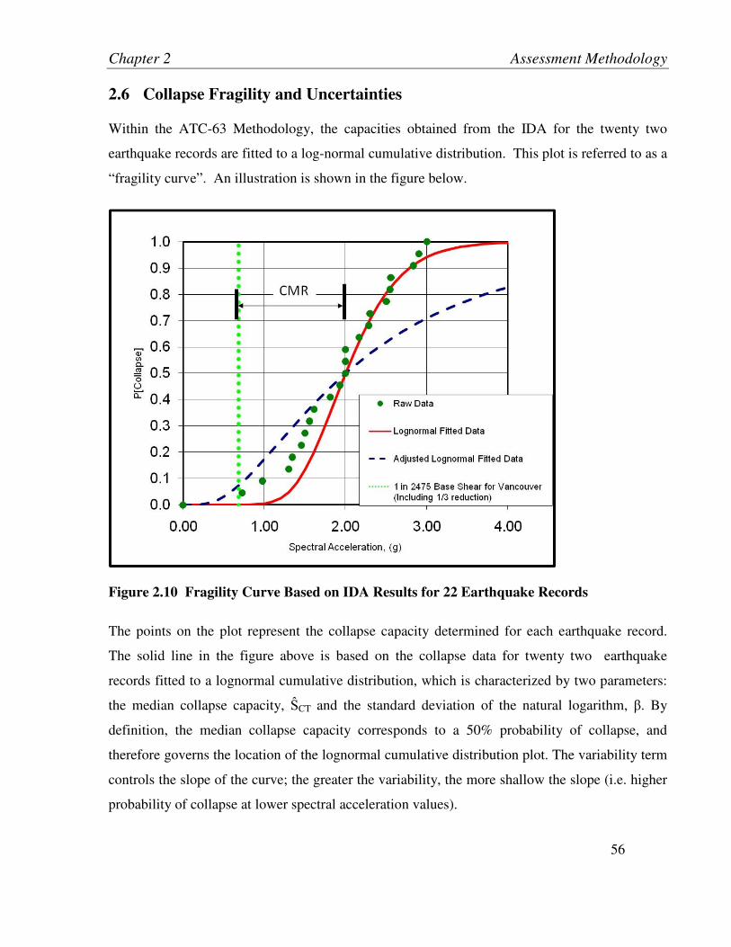
Chapter 2 Assessment Methodology
56
2.6 Collapse Fragility and Uncertainties
Within the ATC-63 Methodology, the capacities obtained from the IDA for the twenty two
earthquake records are fitted to a log-normal cumulative distribution. This plot is referred to as a
“fragility curve”. An illustration is shown in the figure below.
Figure 2.10 Fragility Curve Based on IDA Results for 22 Earthquake Records
The points on the plot represent the collapse capacity determined for each earthquake record.
The solid line in the figure above is based on the collapse data for twenty two earthquake
records fitted to a lognormal cumulative distribution, which is characterized by two parameters:
the median collapse capacity, ŜCT and the standard deviation of the natural logarithm, β. By
definition, the median collapse capacity corresponds to a 50% probability of collapse, and
therefore governs the location of the lognormal cumulative distribution plot. The variability term
controls the slope of the curve; the greater the variability, the more shallow the slope (i.e. higher
probability of collapse at lower spectral acceleration values).

Chapter 2 Assessment Methodology
57
Within the ATC-63 Methodology, the standard deviation of the natural logarithm, β, is identified
by a subscript that refers to the source of the variability. The variability in the solid curve is a
result of variability in response between different earthquakes, and is termed “Record to Record”
variability, and is expressed as βRTR. The dotted line shown in Figure 2.10 incorporates
variability from modeling uncertainties (βMDL), uncertainties related to the degree to which the
design and characterisation of the structure arch-type represent actual structures in the field,
(referred to as uncertainties related to design requirements, (βDR), and uncertainties related to test
data (βTD). The ATC-63 Methodology assumes a fixed value for the record-to-record
uncertainty, βRTR=0.4. However, within this study, the βRTR is determined directly from the
results of the analysis. For the remaining sources of variability, the uncertainty is quantified by
assigning values based on a quality rating as follows: β=0.2 for “superior”, β=0.3 for “good”,
β=0.45 for “fair”, and β=0.65 for “poor”. The various sources of uncertainty are combined as
follows:
2222TDDRMDLRTRTOT βββββ +++= (2.1)
The dotted line represents the collapse fragility curve for the structure incorporating all sources
of variability. From the collapse fragility curve, the probability of structural collapse at the
design earthquake level can be determined.
2.7 Median Collapse Adjustment for Spectral Shape
The spectral shape of rare ground motions is peaked near the period of interest, causing these
ground motions to be less damaging than other records when scaled to the same intensity (Baker
and Cornell, 2006). The ground motion records used in the ATC-63 Methodology are from
earthquakes of magnitude 6.5 to 7.6 on the Richter scale and do not incorporate this spectral
shape, and are thus likely to result in under-prediction of the collapse capacity of a structure (i.e.
conservative prediction of the probability of collapse). To correct for this effect, the ATC-63
Methodology provides an adjustment factor, termed a “spectral shape factor” for the median
collapse spectral acceleration determined from IDA. The spectral shape factor depends on the
seismicity of the region of interest, and the anticipated degree of softening of the initial building
period during response. Within the 70% draft of ATC-63, the building deformation capacity was

Chapter 2 Assessment Methodology
58
assumed to be related to the R factor for the structural system, which is incorporated in the
method to determine the spectral shape factor. For high seismicity regions (areas of interest
within this study), the spectral shape factor from the 70% draft of ATC-63 was as follows:
Table 2.3 Spectral Shape Factor for Different R Factors
R Factor 2 2.5 3 4
Spectral Shape Factor 1.00 1.05 1.1 1.2
As can be observed from the above table, spectral shape has little influence on structural collapse
capacity for the range of R-factors likely to be relevant within this study (i.e. 1 ≤ R ≤ 3).
The manner in which the Spectral Shape Factors are determined has changed for the 90% Draft
of the ATC-63 Methodology; ductility is used instead of the R factor. However this cannot be
used for the rocking or sliding system, since there is no bound on ductility. The spectral shape
factors from the 70% Draft have been adopted for this study.
2.8 Evaluation and Acceptance Criteria
The collapse capacity of a structure is evaluated in accordance with the methodology outlined
above. Once a collapse fragility curve is developed for a structure, the probability of structural
collapse at the design earthquake level can be determined. If this probability is above the desired
value, the R-factor used to design the structure arch-type is reduced, the structure is re-designed,
and the analysis process is repeated. Once the probability of collapse is above the desired value,
the R-factor used can be assumed to be adequate.
For the purposes of this study, a maximum probability of collapse of 0.10 is adopted for the
design earthquake with an annual excedence frequency of 1 in 2475. It is important to note that
this criteria is more stringent that recommended by the ATC-63 Methodology. Within the ATC-
63 Methodology, the acceptable maximum probability of collapse is 0.2 within a performance

Chapter 2 Assessment Methodology
59
group and 0.1 on average for the performance group. Since there are no performance groups
within this study, the more stringent requirement has been adopted.
60
3 INVESTIGATION OF MECHANISM ALTERNATIVES
3.1 Analysis Model Configuration
Based on testing of standard EM5 wall-to-slab connectors (Devine, 2008), it is likely that strong
ground shaking would result in failure of the wall-to-slab connections with limited energy
dissipation at the connection. Failure of the connection may subsequently lead to either sliding
or rocking of the wall panels on the foundation. This section describes efforts to explore the
nonlinear response of tilt-up buildings after failure of the slab-to-wall connection, and to
investigate the preferred mode of response for the design of new tilt-up buildings.
Three types of energy dissipating mechanisms were investigated for tilt-up structures: sliding of
wall panels, rocking of wall panels, and frame mechanisms. In addition, an attempt was made to
investigate the response of a building designed according to current practice. In order to
investigate alternatives for an energy dissipating mechanism for tilt-up buildings, the two
archetypical buildings discussed in Section 2.4 were considered. The design of the wall panels
and connections was modified to ensure the building response displayed the desired mechanism.
3.1.1 Conventional Building
To investigate the response of a building designed in accordance with current practice,
Archetypical System 1 was considered. Available information on existing connections was
gathered (refer to Section 1.2.3) and the system was initially studied by conducting pushover
analyses on two adjacent wall panels connected to each other and to the floor slab of the
building. Figure 3.1 below illustrates the two-panel model.

Chapter 3 Investigation of Mechanism Alternatives
61
Figure 3.1 Two-Panel Model for Pushover Analyses
Combined backbone curves were constructed for EM3 to EM5 connections and EM5 to EM5
connection based on available test data for individual connectors (see Section 1.2.3). While
gathering available information on connector test data, it was determined that there had not been
any tests conducted on the EM3 to EM5 connections at the base of the panels for uplift due to
rocking. It is expected that there would be an interaction for both strength and stiffness of this
connection between uplift and shear. Due to the lack of this information, a meaningful analysis
of a building designed according to current practice was not possible. An attempt was made to
conduct a pushover analysis of the above model, based on an assumed behaviour for the EM3 to
EM5 connector in uplift and an assumed interaction relationship between uplift and shear.
Unfortunately, considerable difficulty was encountered in attempting to accurately model the bi-
directional response expected for the EM3 to EM5 connection with different load-deformation

Chapter 3 Investigation of Mechanism Alternatives
62
relationships in each direction and interaction between the two directions in Perform (Computers
and Structures, 2006). A discussion of the types of elements that were used and the problems
encountered is included in Appendix A. After the data is available from tests on the uplift
performance of the EM3 to EM5 connection (Devine 2008), future analytical research should
focus on the development of an interaction model and the assessment of current tilt-up
construction with slab-to-wall connections.
3.1.2 Model 1: Sliding Mechanism
To investigate the response of a building designed to have a failure mechanism characterized by
in-plane sliding of the wall panels, Archetypical System 1 was considered but the connection
layout was modified. It was assumed that all panels were connected to adjacent panels and with
no connections at the base. A 3D model was constructed in Perform to carry out the analyses.
The model is illustrated in Figure 3.2 below.
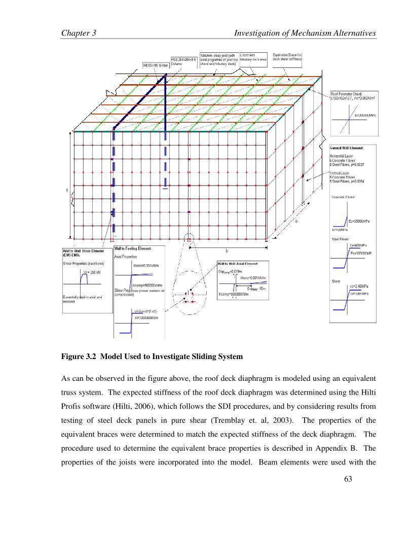
Chapter 3 Investigation of Mechanism Alternatives
63
Figure 3.2 Model Used to Investigate Sliding System
As can be observed in the figure above, the roof deck diaphragm is modeled using an equivalent
truss system. The expected stiffness of the roof deck diaphragm was determined using the Hilti
Profis software (Hilti, 2006), which follows the SDI procedures, and by considering results from
testing of steel deck panels in pure shear (Tremblay et. al, 2003). The properties of the
equivalent braces were determined to match the expected stiffness of the deck diaphragm. The
procedure used to determine the equivalent brace properties is described in Appendix B. The
properties of the joists were incorporated into the model. Beam elements were used with the
Chapter 3 Investigation of Mechanism Alternatives
64
moment of inertia of the full joist, and axial properties of the top chord of the joist only (the
bottom chord is assumed not to participate in the deck diaphragm behaviour). The properties of
the deck in the direction perpendicular to the joist span direction were incorporated into the
model as tension/compression members with axial properties from an equivalent deck area. The
perimeter angle was also incorporated into the model as a beam element. Girders and columns
were incorporated as beam elements. The steel columns were assumed to be fixed at the base
since they normally are supported on a concrete pedestal below the slab level.
The roof system was assumed to be elastic for the purposes of this study. This assumption was
made to ensure that non-linear behaviour occurred in the walls, which are the focus of this study,
and not in the roof diaphragm. When two non-linear components (with limited strain hardening)
are acting in series, as is the case in a typical tilt-up building, if one component yields, the other
will remain elastic. Nonlinear behaviour of the steel deck diaphragm is outside the scope of this
study.
Vertical loads from the roof were treated as concentrated loads on the joists at each joist node.
As shown in the above figure, joists span between the girders and the wall panels. Girders span
between columns. Columns were provided adjacent to end wall panels to ensure that vertical
loads were not transferred from the girders to the end wall panels. This is consistent with
conventional design practice.
The wall panels were modeled as fibre elements with elastic-perfectly-plastic (EPP) material
properties for the concrete and reinforcing steel fibres, with an Elastic Modulus of 30000MPa for
concrete and 200000MPa for steel. At the base of the wall panels, contact elements were
provided (Friction Pendulum elements used in Perform) to model the friction contact between
the wall panels and the footings. The properties for these elements include a large stiffness in
compression, a very small stiffness in tension, and a large stiffness in shear. The shear resistance
is proportional to the applied vertical compression load. The constant of proportionality is the
friction factor, which was selected to ensure the lateral force required to initiate wall sliding was
the same as the lateral force required to initiate wall rocking in the rocking model (see Section
3.1.3). This was done to allow direct comparison between the results of the two mechanisms. A
friction factor of 0.42 was used for comparison purposes.
Chapter 3 Investigation of Mechanism Alternatives
65
The wall panels were fixed in out-of-plane translation along the base. This assumption was
considered valid since in practice, wall panels are erected using “locating pins” (refer to Figure
1.7) consisting of short stubs of large diameter reinforcing steel extending up from the footing
used as a guide during installation of the panels. Adjacent panels were connected using short
beam elements to model the EM5-EM5 connections, incorporating the backbone curve (refer to
Appendix B) developed for those connections.
A Rayleigh damping value of 3% was used for the model at vibration periods of 0.2 and 1.5
times the first mode period. The values for the periods were adopted based on a
recommendation by the ATC-63 Methodology. The damping value was adopted based on a
recommendation in Chopra (2000).
3.1.3 Model 2: Rocking Mechanism
To investigate the response of a building designed to have a failure mechanism characterized by
in-plane rocking of the wall panels, Archetypical System 1 was considered but the connection
layout was modified. It was assumed that all panels were not connected to adjacent panels and
thus able to rock independently. The panels were also assumed to be connected at the base with
connections that would stop sliding from occurring but would allow rocking of the panels to
occur (refer to Section 3.6). A 3D model was constructed in Perform to carry out the analyses.
The model used was very similar to the one used to study the sliding mechanism. The main
differences are that the corner nodes of the panels are fixed in horizontal translation (in-plane
and out-of-plane displacement) and there are no EM5-EM5 connections between panels for the
rocking model. This allows the individual panels to rock on their corner nodes.
3.1.4 Model 3: Frame Mechanism
To investigate the response of a building designed to have a failure mechanism characterized by
in-plane bending of the legs in wall panels with openings, Archetypical System 2 was
considered. A 3D model was constructed in Perform to carry out the analyses. As shown in the
layout of Archetype 2 (Figure 2.7), panels with openings are incorporated along the short axis of
the building. To model the panels with openings, fibre elements are used with EPP material
properties for concrete and steel fibres, as well as for shear behaviour. For walls in the long axis

Chapter 3 Investigation of Mechanism Alternatives
66
of the building, rocking panels were assumed. The rocking panels were modeled as described
previously. Figure 3.3 below illustrates the analytical model used.
Figure 3.3 Model Used to Investigate Frame Mechanism
The frame mechanism was considered separately from the sliding or rocking mechanism, since it
only applies to buildings with large openings in wall panels. As such, the yield strengths of the
concrete and reinforcing steel in the panel legs were not modified to result in a base shear equal
to the sliding and rocking models. The material properties were based on realistic values.
One important limitation in the modeling of the frame mechanism was the lack of available
information on the behaviour of the panel to slab connections (refer to EM5 connection shown in
Chapter 3 Investigation of Mechanism Alternatives
67
Figure 1.6) at the base. Although some information is available on the behaviour of the
connections in the horizontal directions, both in-plane and out-of-plane (Lemieux et. al. 1998),
there is no information available on their behaviour in uplift. An experimental program is
currently underway at UBC (Devine 2008) to investigate the behaviour of EM5 panel to slab
connections in uplift and to investigate interaction relationships between shear and uplift. For
the modeling carried out in this study, a pinned base was assumed at each of the panel legs.
3.2 Model Verification
The analytical models used to carry out the investigations were verified in several ways. Where
possible, results from simple analyses were compared with hand calculations. This was done for
gravity loads, as well as for pushover analysis. The fundamental mode determined from modal
analysis was compared with a simple estimate using the ASCE 41-06 equation (ASCE, 2007) in
Section 3.2.1. In addition, the displaced shape of the models was observed for various load cases
in an effort to detect erroneous behaviour.
3.2.1 Model 1: Sliding Mechanism
Several aspects of the model were checked. The calculated weight of the building (9243 kN)
was compared to the dead load reaction from the analysis (9210 kN). Results from a modal
analysis indicated the first mode period of the model was 0.58 seconds, with 56% of the total
building mass participating in this mode. The first mode occurs in the direction of the short axis
of the building. The next important mode for the model was the third mode, with a period of
0.33 seconds, with 38% of the mass participating. The third mode occurs in the direction of the
longer axis of the building. Figure 3.4 below illustrates the first mode shape as determined
using Perform.

Chapter 3 Investigation of Mechanism Alternatives
68
Figure 3.4 First Mode (Period = 0.58 seconds)
The first mode period of the structure was also estimated using the equation recommended by
ASCE 41-06 for buildings with flexible diaphragms:
5.0)78.01.0(1 dwT ∆+∆=
(3.1)
Where ∆w and ∆d are in-plane wall and diaphragm displacements in inches, due to a distributed
lateral load in the direction under consideration, equal to the weight of the diaphragm. Using the
above equation, the first mode period was calculated to be 0.41 seconds, which is considerably
shorter than the first mode period determined from the modal analysis. However, when the
ASCE 41-06 estimate was modified by considering half the weight of the out-of-plane walls, the
resulting period was 0.63 seconds, which is approximately 9% longer than the period determined
from modal analysis. The inclusion of half the weight of the out-of-plane walls was thought to
be reasonable, since it is included in the seismic demands in standard practice. Also, from
observing the shape of the first mode (Figure 3.4) it is obvious that some of the inertial forces
from the mass of the out-of-plane walls must be transferred into the diaphragm, and hence, will
participate in the mode.

Chapter 3 Investigation of Mechanism Alternatives
69
It is interesting to note both the first mode period determined from analysis (0.58 seconds) and
using the ASCE 41-06 formula (0.63 seconds) are considerably longer than the first mode period
determined using the NBCC 2005 formula (0.26 seconds) or the IBC 2003 formula (0.11
seconds).
Pushover analyses were conducted for the sliding model in the direction of each primary axis of
the building. The shape of the load distribution used for the pushover analyses was based on the
fundamental mode in the direction of each primary axis. For each pushover analysis, the total
base shear resisted by the in-plane wall panels was plotted against the drift at the middle of the
roof. The base shear resisted by the in-plane walls is expressed as a percentage of the assumed
tributary building weight for the direction of interest including the weight of the roof, half the
weight of the out-of-plane walls, and the full weight of the in-plane walls – identical to the
tributary weight assumed in practice for calculation of the design base shear. This was done to
allow comparison of the pushover plot with the design base shear. To check the results from
Perform, the ultimate base shear for the building was estimated using hand calculations. Figure
3.5 below illustrates the results of the pushover analysis in the direction of the short axis of the
building. The roof drift is expressed in terms of the displacement at the middle of the roof
divided by the height of the building.
Figure 3.5 Sliding Mechanism - Pushover Analysis Along Short Axis of Building

Chapter 3 Investigation of Mechanism Alternatives
70
As can be observed, the results from Perform match closely with the ultimate base shear
estimated using hand calculations. Figure 3.6 below illustrates the displaced shape of the model
during the pushover analysis in direction of the short axis of the building.
Figure 3.6 Sliding Mechanism – Displaced Shape for Pushover Along Short Axis of Building
As can be observed in Figure 3.6 above, the response of the model in the direction of the long
axis and short axis of the building has been decoupled. There are no connections provided
between adjacent corner panels. This is necessary to ensure a sliding mechanism can develop.
Figure 3.7 below illustrates the results of the pushover analysis in the direction of the long axis
of the building.
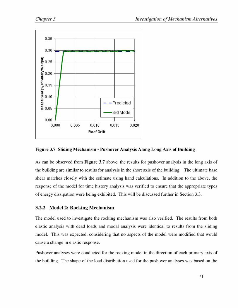
Chapter 3 Investigation of Mechanism Alternatives
71
Figure 3.7 Sliding Mechanism - Pushover Analysis Along Long Axis of Building
As can be observed from Figure 3.7 above, the results for pushover analysis in the long axis of
the building are similar to results for analysis in the short axis of the building. The ultimate base
shear matches closely with the estimate using hand calculations. In addition to the above, the
response of the model for time history analysis was verified to ensure that the appropriate types
of energy dissipation were being exhibited. This will be discussed further in Section 3.3.
3.2.2 Model 2: Rocking Mechanism
The model used to investigate the rocking mechanism was also verified. The results from both
elastic analysis with dead loads and modal analysis were identical to results from the sliding
model. This was expected, considering that no aspects of the model were modified that would
cause a change in elastic response.
Pushover analyses were conducted for the rocking model in the direction of each primary axis of
the building. The shape of the load distribution used for the pushover analyses was based on the
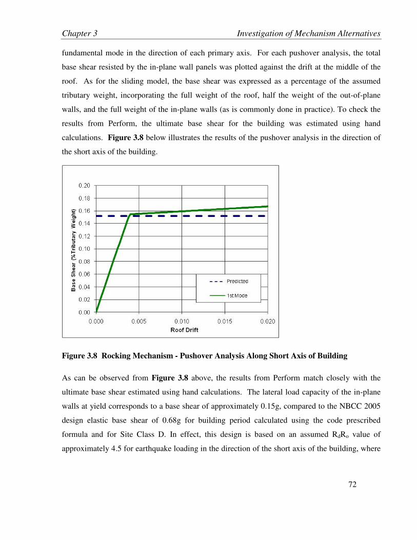
Chapter 3 Investigation of Mechanism Alternatives
72
fundamental mode in the direction of each primary axis. For each pushover analysis, the total
base shear resisted by the in-plane wall panels was plotted against the drift at the middle of the
roof. As for the sliding model, the base shear was expressed as a percentage of the assumed
tributary weight, incorporating the full weight of the roof, half the weight of the out-of-plane
walls, and the full weight of the in-plane walls (as is commonly done in practice). To check the
results from Perform, the ultimate base shear for the building was estimated using hand
calculations. Figure 3.8 below illustrates the results of the pushover analysis in the direction of
the short axis of the building.
Figure 3.8 Rocking Mechanism - Pushover Analysis Along Short Axis of Building
As can be observed from Figure 3.8 above, the results from Perform match closely with the
ultimate base shear estimated using hand calculations. The lateral load capacity of the in-plane
walls at yield corresponds to a base shear of approximately 0.15g, compared to the NBCC 2005
design elastic base shear of 0.68g for building period calculated using the code prescribed
formula and for Site Class D. In effect, this design is based on an assumed RdRo value of
approximately 4.5 for earthquake loading in the direction of the short axis of the building, where

Chapter 3 Investigation of Mechanism Alternatives
73
RdRo is defined as the design elastic base shear divided by the yield strength of the building (i.e.
RdRo =Sa(T1)Wtributary/Vy).
Since the calculated period of the building is relatively short (0.26 seconds), the NBCC 2005
limits the base shear to two-thirds of the peak design spectral acceleration. It is interesting to
note that if the first mode period from the model is used (approximately 0.6 seconds) instead of
the NBCC 2005 calculated period, the design base shear reduces to 0.64g, resulting in a slightly
smaller assumed RdRo value of 4.3. Figure 3.9 below illustrates the displaced shape of the
model during the pushover analysis in direction of the short axis of the building.
Figure 3.9 Rocking Mechanism – Displaced Shape for Pushover Along Short Axis of
Building
Similarly to the sliding model, the response in the direction of the long axis and short axis of the
building has been decoupled. There are no connections provided between adjacent corner
panels. This is necessary to ensure a rocking mechanism can develop.
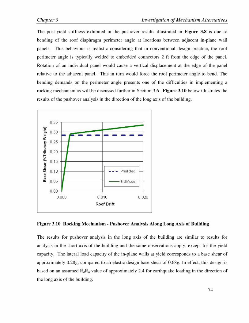
Chapter 3 Investigation of Mechanism Alternatives
74
The post-yield stiffness exhibited in the pushover results illustrated in Figure 3.8 is due to
bending of the roof diaphragm perimeter angle at locations between adjacent in-plane wall
panels. This behaviour is realistic considering that in conventional design practice, the roof
perimeter angle is typically welded to embedded connectors 2 ft from the edge of the panel.
Rotation of an individual panel would cause a vertical displacement at the edge of the panel
relative to the adjacent panel. This in turn would force the roof perimeter angle to bend. The
bending demands on the perimeter angle presents one of the difficulties in implementing a
rocking mechanism as will be discussed further in Section 3.6. Figure 3.10 below illustrates the
results of the pushover analysis in the direction of the long axis of the building.
Figure 3.10 Rocking Mechanism - Pushover Analysis Along Long Axis of Building
The results for pushover analysis in the long axis of the building are similar to results for
analysis in the short axis of the building and the same observations apply, except for the yield
capacity. The lateral load capacity of the in-plane walls at yield corresponds to a base shear of
approximately 0.28g, compared to an elastic design base shear of 0.68g. In effect, this design is
based on an assumed RdRo value of approximately 2.4 for earthquake loading in the direction of
the long axis of the building.

Chapter 3 Investigation of Mechanism Alternatives
75
3.2.3 Model 3: Frame Mechanism
Various aspects of the model used to investigate the frame mechanism were verified. The
calculated weight of the building (9053 kN) was compared to the dead load reaction from the
analysis (9010 kN). Results from a modal analysis indicated the first mode period of the model
was 0.61 seconds, with 55% of the total building mass participating in the mode. The first mode
occurs in the direction of the short axis of the building. The next important mode for the model
was the third mode, with a period of 0.34 seconds, with 42% of the mass participating. The third
mode occurs in the direction of the longer axis of the building. The two modal periods and
associated mass participation given above are very similar to the modal periods determined for
Models 1 and 2. This is expected for the third mode of the building, since for all the models,
solid panels are used on the long axis of the building. For the first mode, this suggests that even
for a building incorporating panels with large openings, the elastic response is predominantly
governed by the roof deck diaphragm.
For the frame model, results from static reversed-cyclic analysis of a beam-column subassembly
(refer to Figure 1.14 for details of the geometry and reinforcing steel) were compared with
experimental test results from Dew et al. (2001), as illustrated in Figure 3.11 below.

Chapter 3 Investigation of Mechanism Alternatives
76
Figure 3.11 Frame Mechanism – Force-Displacement Plot for Beam-Column
Subassembly: Comparison of Analytical and Experimental Results (Dew et al., 2001)
The analytical model matches the experimental data reasonably well for strength and stiffness.
The displacement capacity displayed by the Perform model is less than that shown by the
experimental results. The discrepancy here is likely due to a difference in the ultimate strain
for the steel reinforcement. An ultimate strain of 0.05 was selected for the Perform 3D model,
based on the limit recommended by ASCE 41 (ASCE, 2007) for reinforcing steel bars
undergoing cyclical loading. Similar to many other limits in ASCE 41, 0.05 is likely
conservative, and hence it is not surprising that the test was able to exceed the displacement
capacity implied by the model.
For Archetypical System 2, a larger leg was required to meet the design requirements than was
used in Dew et al. (2001). The leg dimensions used in this current study are proportionally
similar to the leg used in the experimental study, with width: thickness ratios of 4.2 for both and
length: width ratios of 3.6 for both. In Figure 3.12 below, the results from Perform 3D are
compared with results from hand calculations using a tri-linear moment curvature model
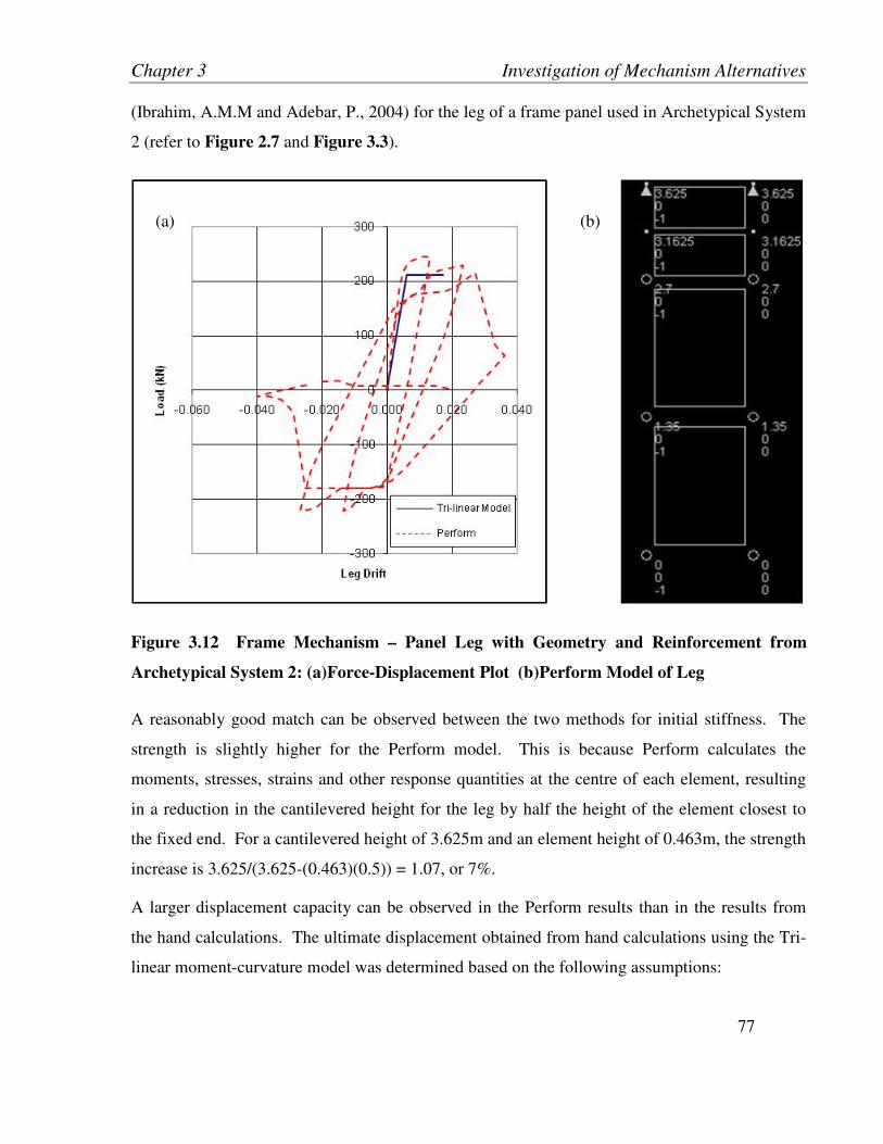
Chapter 3 Investigation of Mechanism Alternatives
77
(Ibrahim, A.M.M and Adebar, P., 2004) for the leg of a frame panel used in Archetypical System
2 (refer to Figure 2.7 and Figure 3.3).
Figure 3.12 Frame Mechanism – Panel Leg with Geometry and Reinforcement from
Archetypical System 2: (a)Force-Displacement Plot (b)Perform Model of Leg
A reasonably good match can be observed between the two methods for initial stiffness. The
strength is slightly higher for the Perform model. This is because Perform calculates the
moments, stresses, strains and other response quantities at the centre of each element, resulting
in a reduction in the cantilevered height for the leg by half the height of the element closest to
the fixed end. For a cantilevered height of 3.625m and an element height of 0.463m, the strength
increase is 3.625/(3.625-(0.463)(0.5)) = 1.07, or 7%.
A larger displacement capacity can be observed in the Perform results than in the results from
the hand calculations. The ultimate displacement obtained from hand calculations using the Tri-
linear moment-curvature model was determined based on the following assumptions:
(a) (b)
Chapter 3 Investigation of Mechanism Alternatives
78
• Distance to section neutral axis determined based on compressive stress block assuming
four of the five rows of bars yielding in tension.
• Ultimate curvature obtained by considering the ultimate concrete strain of 0.0035 divided
by the distance to the neutral axis.
• Inelastic displacement determined assuming plastic hinge length equal to the section
depth.
• Elastic displacement determined using cracked moment of inertia.
The material models used in Perform include strength degradation and can accommodate strains
well beyond the ultimate strains with reduced strengths. Also, the Perform model accounts for
cyclical degradation by decreasing the stiffness of the reinforcing steel with each cycle. Both of
these reasons account for the greater displacements observed in the Perform model.
In the archetypical building and in common practice, legs of adjacent panels are connected
together with panel to panel connectors, providing shear transfer between the legs and effectively
doubling the width of the leg section, thereby changing its characteristics dramatically. Figure
3.13 below illustrates both a moment-curvature plot and a force-displacement plot to compare
the behaviour of two legs from adjacent frame panels connected together with the behaviour of
one panel leg, based on results from hand calculations.
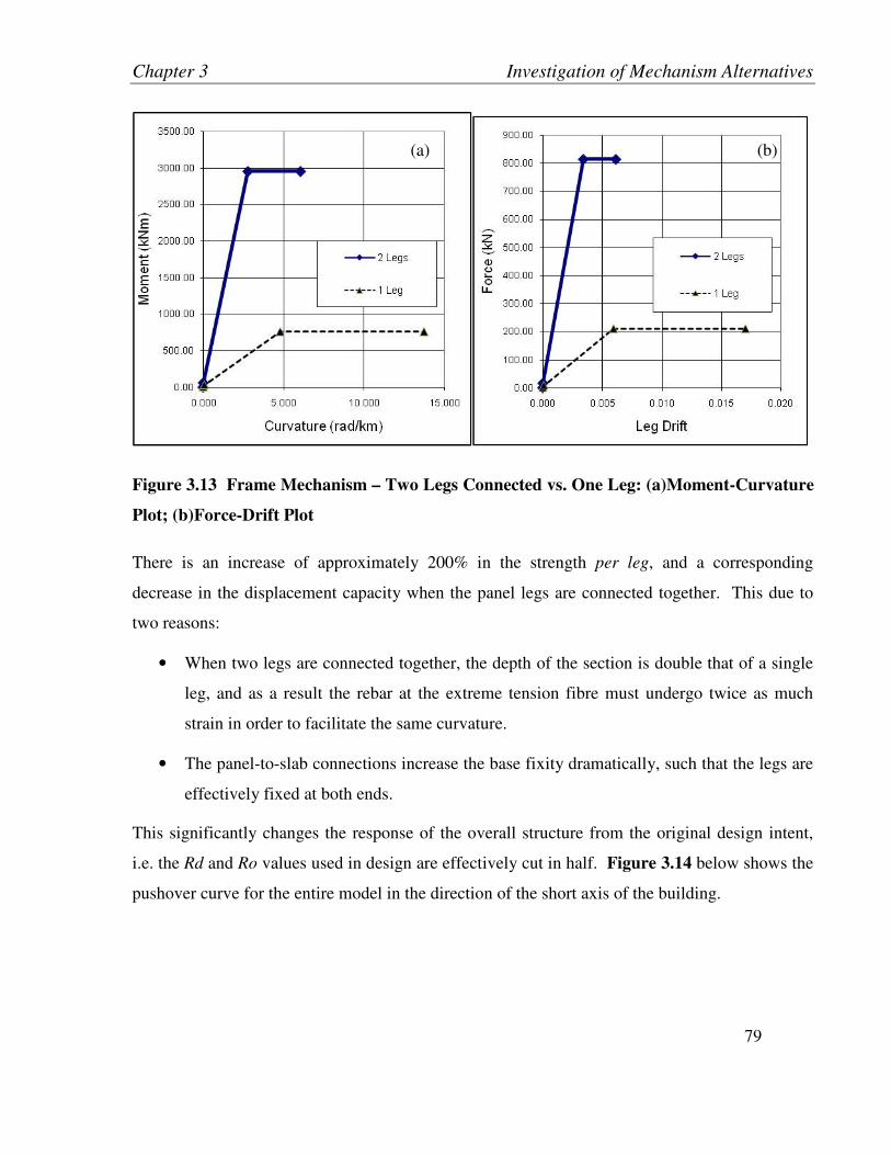
Chapter 3 Investigation of Mechanism Alternatives
79
Figure 3.13 Frame Mechanism – Two Legs Connected vs. One Leg: (a)Moment-Curvature
Plot; (b)Force-Drift Plot
There is an increase of approximately 200% in the strength per leg, and a corresponding
decrease in the displacement capacity when the panel legs are connected together. This due to
two reasons:
• When two legs are connected together, the depth of the section is double that of a single
leg, and as a result the rebar at the extreme tension fibre must undergo twice as much
strain in order to facilitate the same curvature.
• The panel-to-slab connections increase the base fixity dramatically, such that the legs are
effectively fixed at both ends.
This significantly changes the response of the overall structure from the original design intent,
i.e. the Rd and Ro values used in design are effectively cut in half. Figure 3.14 below shows the
pushover curve for the entire model in the direction of the short axis of the building.
(a) (b)

Chapter 3 Investigation of Mechanism Alternatives
80
Figure 3.14 Frame Mechanism – Pushover Analysis Along Short Building Axis
Due to the connectivity between adjacent panels, the resistance of the building to lateral loading
increases considerably. The design base shear for the building for in-plane flexural strength of
the panel legs (based on Rd=1.5, Ro=1.3) was 0.35g. As can be seen in Figure 3.14 above, the
actual base shear resisted by the building is on the order of 0.87g. This is effectively a 250%
increase in strength. The Pushover analyses were conducted for the frame model only in the
direction of the short axis of the building, since the long axis has solid panels similar to the
rocking model.
3.3 Time History Analysis Results
To observe the distinct characteristics of each mechanism, the results from a time history
analysis for one earthquake applied in the direction of the short axis of the building was
considered for each model. The record considered was from the Northridge earthquake and was
recorded at the Beverly Hills - Mulhol recording station. It constituted the first record in the set

Chapter 3 Investigation of Mechanism Alternatives
81
recommended for use in the ATC-63 Methodology (see Table 2.1) and was obtained from the
PEER-NGA database (http://peer.berkeley.edu/nga/). Two scaling factors were considered in
order to capture the response of the models in both the linear and nonlinear ranges. The record
was scaled in amplitude only such that the 3% damped spectral acceleration at the first mode
period was equal to 0.1g (i.e. Sa(T1) = 0.1g) to investigate the linear response, and 1g to initiate
nonlinear response. The scaling factors required to achieve these intensities were 0.0625 and
0.625 respectively. The breakdown of energy dissipation mechanisms was investigated for each
model.
3.3.1 Model 1: Sliding Mechanism
The response of the sliding model for the record described above can be illustrated by
considering the drift at the centre of the roof (displacement at mid-span divided by the height of
the roof) and the drift at the top of the end wall panels (displacement at top of end walls divided
by the height of the end walls). These two drifts are shown plotted in Figure 3.15 below for
Sa(T1) = 0.1g and 1.0g.
Figure 3.15 Sliding Model – Wall and Roof Drifts for Northridge Earthquake; (a)
Sa(T1)=0.1g; (b) Sa(T1)=1.0g
It can be observed in Figure 3.15 (a) above that the roof essentially governs the response, and
the walls remain elastic. The maximum roof drift is approximately 0.14% (13mm). There is no
(a) (b)
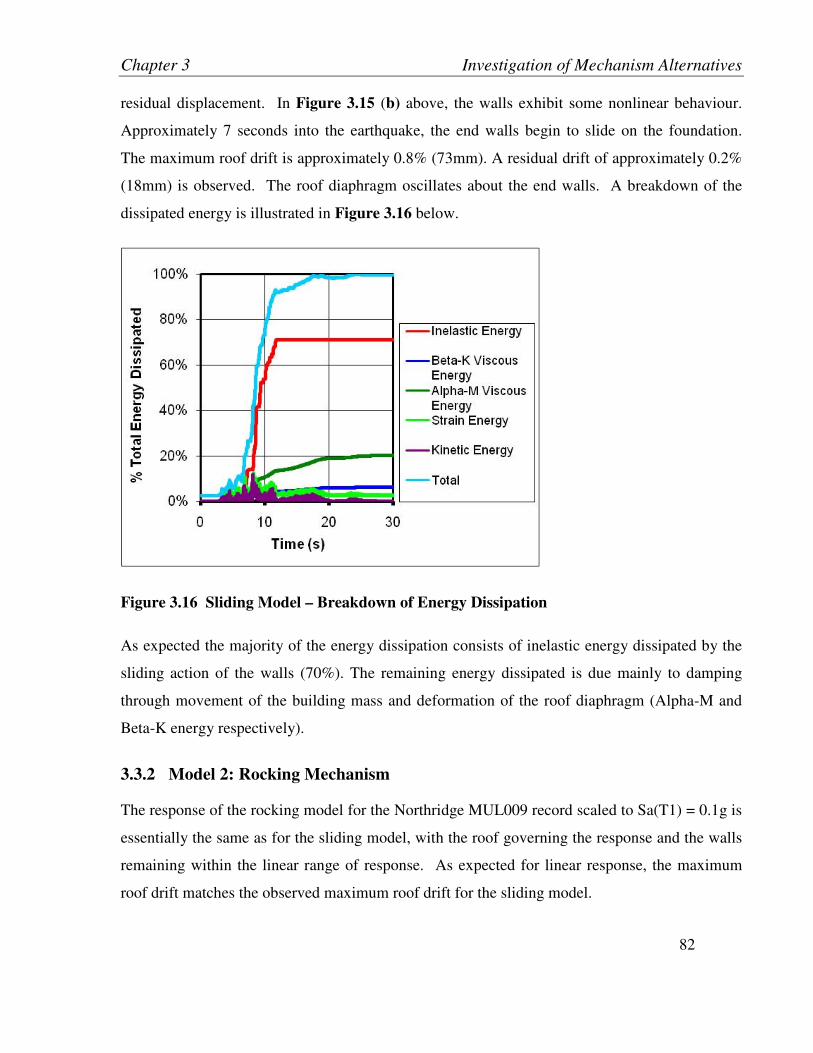
Chapter 3 Investigation of Mechanism Alternatives
82
residual displacement. In Figure 3.15 (b) above, the walls exhibit some nonlinear behaviour.
Approximately 7 seconds into the earthquake, the end walls begin to slide on the foundation.
The maximum roof drift is approximately 0.8% (73mm). A residual drift of approximately 0.2%
(18mm) is observed. The roof diaphragm oscillates about the end walls. A breakdown of the
dissipated energy is illustrated in Figure 3.16 below.
Figure 3.16 Sliding Model – Breakdown of Energy Dissipation
As expected the majority of the energy dissipation consists of inelastic energy dissipated by the
sliding action of the walls (70%). The remaining energy dissipated is due mainly to damping
through movement of the building mass and deformation of the roof diaphragm (Alpha-M and
Beta-K energy respectively).
3.3.2 Model 2: Rocking Mechanism
The response of the rocking model for the Northridge MUL009 record scaled to Sa(T1) = 0.1g is
essentially the same as for the sliding model, with the roof governing the response and the walls
remaining within the linear range of response. As expected for linear response, the maximum
roof drift matches the observed maximum roof drift for the sliding model.

Chapter 3 Investigation of Mechanism Alternatives
83
The drifts at roof centre and top of the end wall panels are shown plotted in Figure 3.17 below
for Sa(T1) = 1.0g.
Figure 3.17 Rocking Model – Wall and Roof Drifts for Northridge Earthquake,
Sa(T1)=1.0g
It can be observed in the figure above that the walls exhibit considerable nonlinear behaviour.
Similar to the sliding model, nonlinear response commences approximately 7 seconds into the
earthquake as the end walls begin to rock on the foundation. Once the earthquake intensity
increases at about 8 seconds, the walls and roof maintain essentially the same displacement for
the majority of the analysis run. The maximum roof drift is approximately 3.2% (290mm).
There is no residual drift; the wall panels always rock back to their original position.
It is important to note that the maximum roof drift is approximately four times the maximum
roof drift observed for the sliding model. This is due to the fact that the rocking mechanism does
not dissipate as much energy as the sliding mechanism. A breakdown of the dissipated energy is
illustrated in Figure 3.18 below.

Chapter 3 Investigation of Mechanism Alternatives
84
Figure 3.18 Rocking Model – Breakdown of Energy Dissipation
Zero inelastic energy is present since the rocking mechanism is nonlinear-elastic and does not
result in the dissipation of hysteretic energy. Approximately 80% of the total energy dissipated
consists of Alpha-M viscous energy dissipated by movement of the building mass. About 15%
of the total energy dissipated consists of Beta-K viscous energy dissipated by deformation of the
roof and wall panels. One form of energy dissipation that is not incorporated in Perform is the
energy that is dissipated when the panel hits the foundation during rocking. This would
represent an additional form of energy dissipation in a real rocking structure.
3.3.3 Model 3: Frame Mechanism
The response of the frame model for the Northridge MUL009 record scaled to Sa(T1) = 0.1g is
essentially the same as for the sliding and rocking models, with the roof governing the response
and the walls remaining elastic. As expected for elastic response, the maximum roof drift

Chapter 3 Investigation of Mechanism Alternatives
85
matches the observed maximum roof drift for the sliding and rocking models. The frame model
does not exhibit any yielding of the in-plane walls for a spectral acceleration Sa(T1) = 1.0g, due
to the greatly increased strength of the panels legs resulting from connection of adjacent panels.
The response of the frame model for the Northridge MUL009 record scaled to Sa(T1) = 3.0g is
illustrated in Figure 3.19 below.
Figure 3.19 Frame Model – Wall and Roof Drifts for Northridge Earthquake, Sa(T1)=3.0g
It can be observed in Figure 3.19 above that the walls exhibit considerable inelastic behaviour.
Observing Figure 3.14, it is evident that the yield drift for the in-plane walls is approximately
0.3% (27mm). Within Figure 3.19 it can be observed that at approximately 3 seconds into the
earthquake, the walls begin to oscillate at a drift of approximately 0.3% (27mm). At
approximately 7 seconds, the wall drift increases to approximately 0.4% (37mm), and eventually
at approximately 12 seconds into the earthquake, the walls fail in-plane due to straining of the
rebar past the ultimate allowable strain. The response shown above is characteristic of the frame
model response when the earthquake intensity is scaled up enough to cause yielding of the walls.
Typically, if the walls yield during an analysis run, the run is terminated due to the model
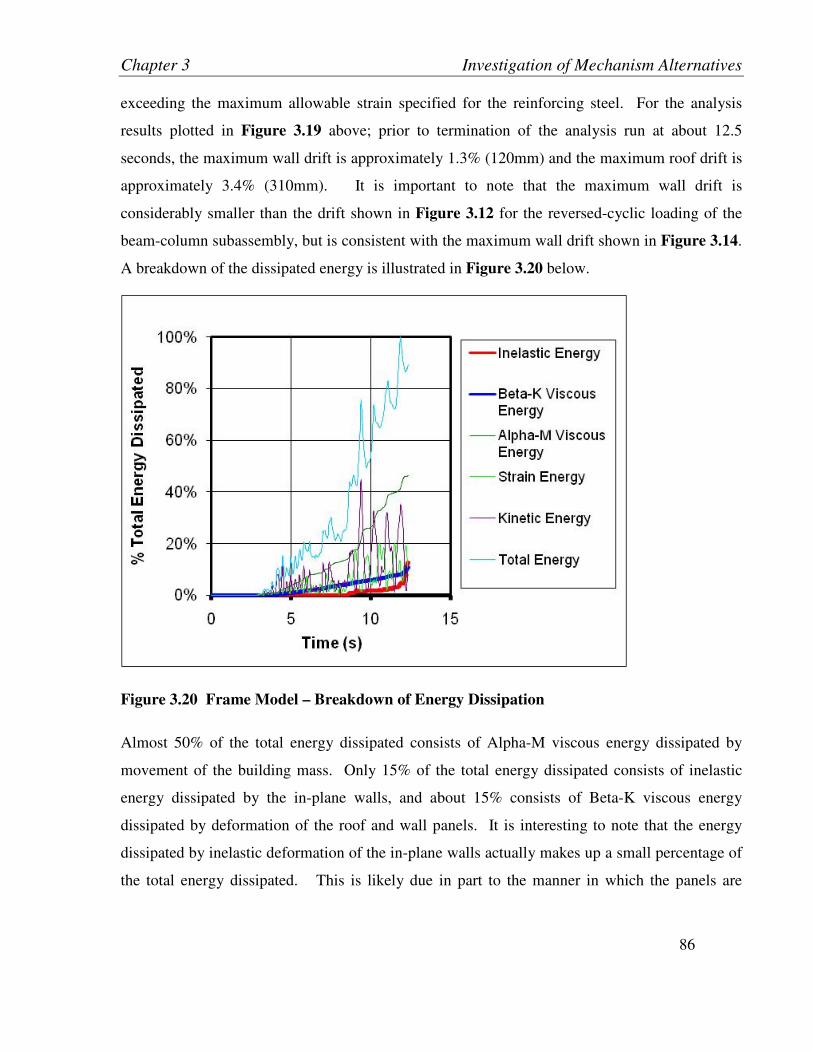
Chapter 3 Investigation of Mechanism Alternatives
86
exceeding the maximum allowable strain specified for the reinforcing steel. For the analysis
results plotted in Figure 3.19 above; prior to termination of the analysis run at about 12.5
seconds, the maximum wall drift is approximately 1.3% (120mm) and the maximum roof drift is
approximately 3.4% (310mm). It is important to note that the maximum wall drift is
considerably smaller than the drift shown in Figure 3.12 for the reversed-cyclic loading of the
beam-column subassembly, but is consistent with the maximum wall drift shown in Figure 3.14.
A breakdown of the dissipated energy is illustrated in Figure 3.20 below.
Figure 3.20 Frame Model – Breakdown of Energy Dissipation
Almost 50% of the total energy dissipated consists of Alpha-M viscous energy dissipated by
movement of the building mass. Only 15% of the total energy dissipated consists of inelastic
energy dissipated by the in-plane walls, and about 15% consists of Beta-K viscous energy
dissipated by deformation of the roof and wall panels. It is interesting to note that the energy
dissipated by inelastic deformation of the in-plane walls actually makes up a small percentage of
the total energy dissipated. This is likely due in part to the manner in which the panels are
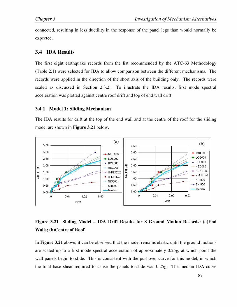
Chapter 3 Investigation of Mechanism Alternatives
87
connected, resulting in less ductility in the response of the panel legs than would normally be
expected.
3.4 IDA Results
The first eight earthquake records from the list recommended by the ATC-63 Methodology
(Table 2.1) were selected for IDA to allow comparison between the different mechanisms. The
records were applied in the direction of the short axis of the building only. The records were
scaled as discussed in Section 2.3.2. To illustrate the IDA results, first mode spectral
acceleration was plotted against centre roof drift and top of end wall drift.
3.4.1 Model 1: Sliding Mechanism
The IDA results for drift at the top of the end wall and at the centre of the roof for the sliding
model are shown in Figure 3.21 below.
Figure 3.21 Sliding Model – IDA Drift Results for 8 Ground Motion Records: (a)End
Walls; (b)Centre of Roof
In Figure 3.21 above, it can be observed that the model remains elastic until the ground motions
are scaled up to a first mode spectral acceleration of approximately 0.25g, at which point the
wall panels begin to slide. This is consistent with the pushover curve for this model, in which
the total base shear required to cause the panels to slide was 0.25g. The median IDA curve
(a) (b)
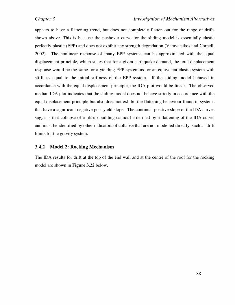
Chapter 3 Investigation of Mechanism Alternatives
88
appears to have a flattening trend, but does not completely flatten out for the range of drifts
shown above. This is because the pushover curve for the sliding model is essentially elastic
perfectly plastic (EPP) and does not exhibit any strength degradation (Vamvatsikos and Cornell,
2002). The nonlinear response of many EPP systems can be approximated with the equal
displacement principle, which states that for a given earthquake demand, the total displacement
response would be the same for a yielding EPP system as for an equivalent elastic system with
stiffness equal to the initial stiffness of the EPP system. If the sliding model behaved in
accordance with the equal displacement principle, the IDA plot would be linear. The observed
median IDA plot indicates that the sliding model does not behave strictly in accordance with the
equal displacement principle but also does not exhibit the flattening behaviour found in systems
that have a significant negative post-yield slope. The continual positive slope of the IDA curves
suggests that collapse of a tilt-up building cannot be defined by a flattening of the IDA curve,
and must be identified by other indicators of collapse that are not modelled directly, such as drift
limits for the gravity system.
3.4.2 Model 2: Rocking Mechanism
The IDA results for drift at the top of the end wall and at the centre of the roof for the rocking
model are shown in Figure 3.22 below.
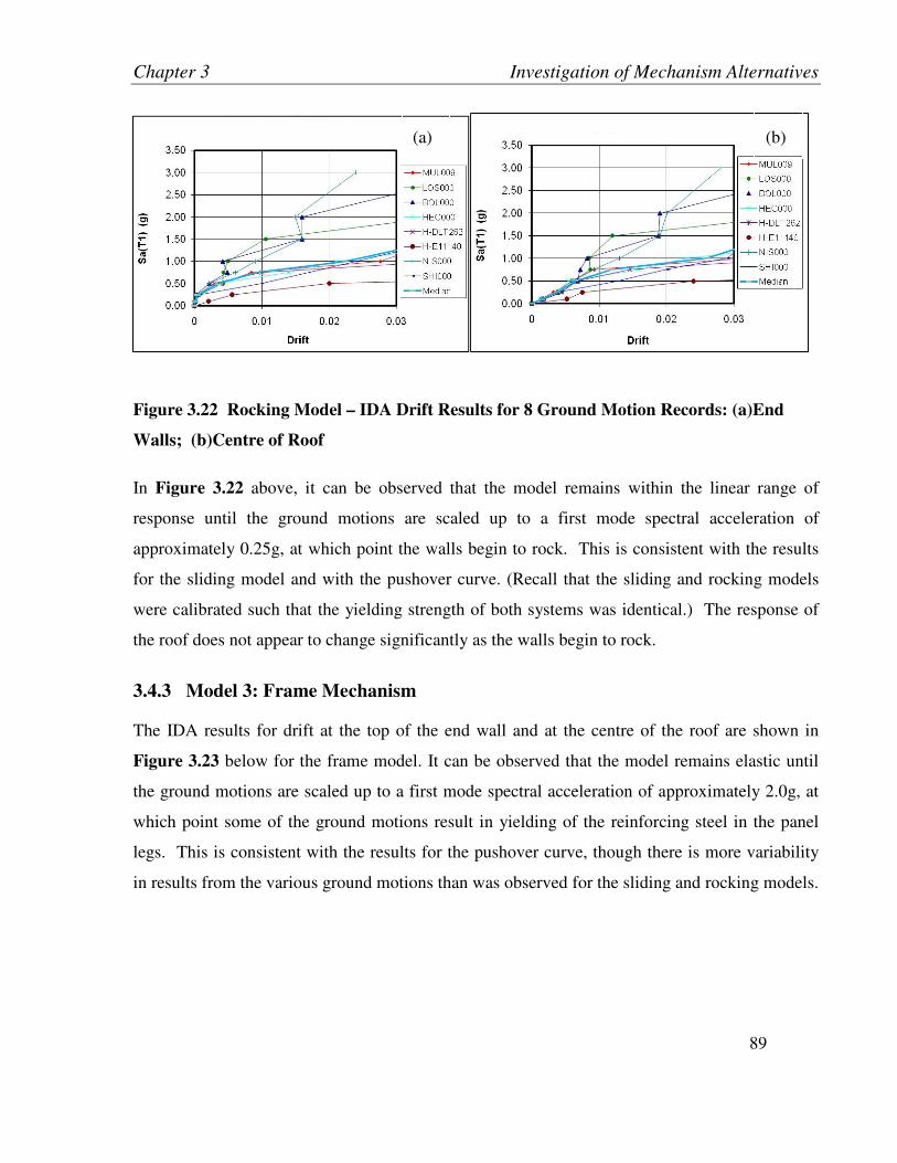
Chapter 3 Investigation of Mechanism Alternatives
89
Figure 3.22 Rocking Model – IDA Drift Results for 8 Ground Motion Records: (a)End
Walls; (b)Centre of Roof
In Figure 3.22 above, it can be observed that the model remains within the linear range of
response until the ground motions are scaled up to a first mode spectral acceleration of
approximately 0.25g, at which point the walls begin to rock. This is consistent with the results
for the sliding model and with the pushover curve. (Recall that the sliding and rocking models
were calibrated such that the yielding strength of both systems was identical.) The response of
the roof does not appear to change significantly as the walls begin to rock.
3.4.3 Model 3: Frame Mechanism
The IDA results for drift at the top of the end wall and at the centre of the roof are shown in
Figure 3.23 below for the frame model. It can be observed that the model remains elastic until
the ground motions are scaled up to a first mode spectral acceleration of approximately 2.0g, at
which point some of the ground motions result in yielding of the reinforcing steel in the panel
legs. This is consistent with the results for the pushover curve, though there is more variability
in results from the various ground motions than was observed for the sliding and rocking models.
(a) (b)
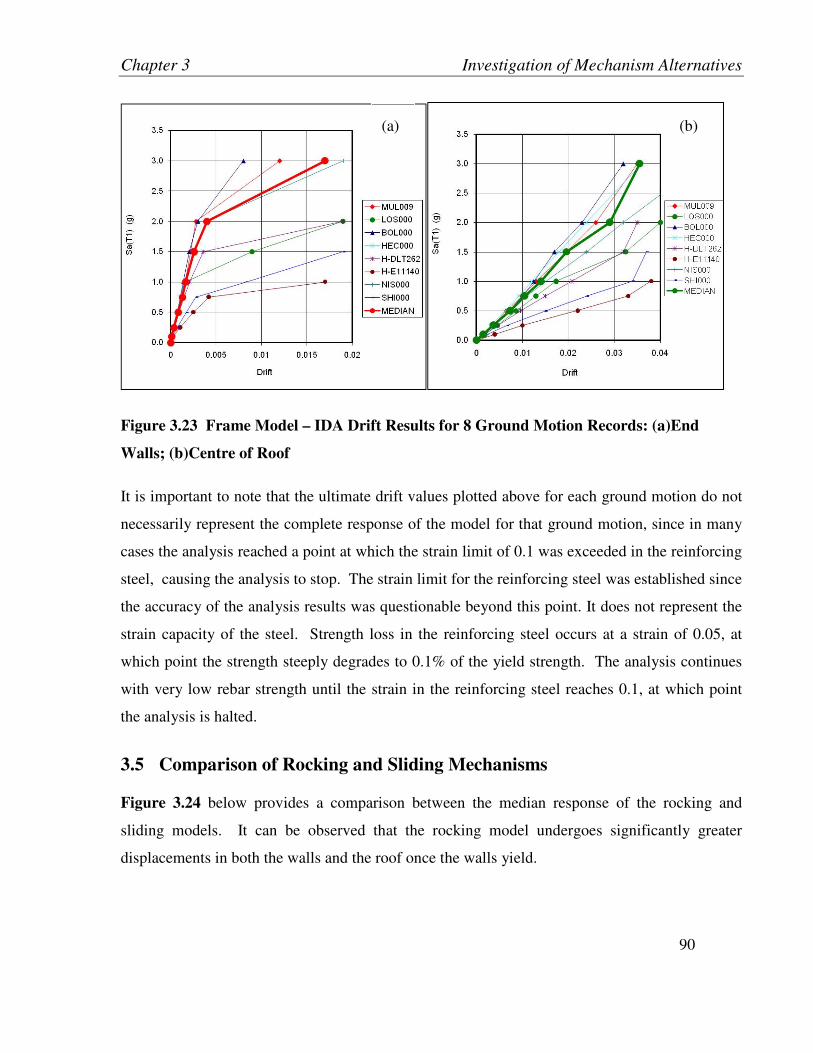
Chapter 3 Investigation of Mechanism Alternatives
90
Figure 3.23 Frame Model – IDA Drift Results for 8 Ground Motion Records: (a)End
Walls; (b)Centre of Roof
It is important to note that the ultimate drift values plotted above for each ground motion do not
necessarily represent the complete response of the model for that ground motion, since in many
cases the analysis reached a point at which the strain limit of 0.1 was exceeded in the reinforcing
steel, causing the analysis to stop. The strain limit for the reinforcing steel was established since
the accuracy of the analysis results was questionable beyond this point. It does not represent the
strain capacity of the steel. Strength loss in the reinforcing steel occurs at a strain of 0.05, at
which point the strength steeply degrades to 0.1% of the yield strength. The analysis continues
with very low rebar strength until the strain in the reinforcing steel reaches 0.1, at which point
the analysis is halted.
3.5 Comparison of Rocking and Sliding Mechanisms
Figure 3.24 below provides a comparison between the median response of the rocking and
sliding models. It can be observed that the rocking model undergoes significantly greater
displacements in both the walls and the roof once the walls yield.
(a) (b)

Chapter 3 Investigation of Mechanism Alternatives
91
Figure 3.24 Sliding and Rocking Models: IDA Drift Results for 8 Ground Motion Records:
(a)End Walls; (b)Centre of Roof
In comparison of the two mechanisms, it is important to consider that the building archetype
used to form a basis for the analytical models is a very simple system. In reality, buildings are
not perfectly rectangular and can have re-entrant corners, or some of the walls may not be
parallel to each other. When these complications in building geometry are considered, the
practicability of the sliding mechanism becomes questionable. Another problem is that the
actual friction factor between the wall panels and the foundation may be difficult to predict. In
addition, due to the residual displacement inherent in the sliding mechanism, earthquake damage
to a building designed to fail in this manner would be difficult to repair. The rocking mechanism
is more practicable for solid panels since it inherently does not involve a residual displacement;
rocking panels always return to their original position. Based on the observations above, the
rocking mechanism and frame mechanism are investigated further using concepts from the ATC-
63 Methodology (refer to Section 2).
3.6 Possible Connection Details for Rocking Mechanism
One of the problems inherent in the rocking mechanism is that adjacent panels that are rocking
will have a differential vertical displacement at their interface. This movement would likely
(a) (b)
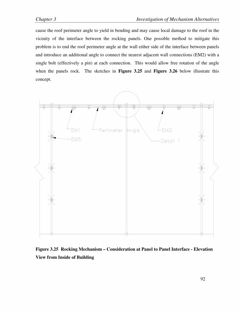
Chapter 3 Investigation of Mechanism Alternatives
92
cause the roof perimeter angle to yield in bending and may cause local damage to the roof in the
vicinity of the interface between the rocking panels. One possible method to mitigate this
problem is to end the roof perimeter angle at the wall either side of the interface between panels
and introduce an additional angle to connect the nearest adjacent wall connections (EM2) with a
single bolt (effectively a pin) at each connection. This would allow free rotation of the angle
when the panels rock. The sketches in Figure 3.25 and Figure 3.26 below illustrate this
concept.
Figure 3.25 Rocking Mechanism – Consideration at Panel to Panel Interface - Elevation
View from Inside of Building

Chapter 3 Investigation of Mechanism Alternatives
93
Figure 3.26 Rocking Mechanism – Consideration at Panel to Panel Interface - Detail at
Panel Interface
Another difficulty with the rocking mechanism is that the type of panel to slab connections
currently used in common practice (EM5 connections – refer to Figure 1.6) would have
significant interaction between uplift and shear. In order for the rocking mechanism to be
feasible in practice, the behaviour of the panel to slab connections in uplift and shear would have
to be de-coupled. One possible solution to this problem is to provide two sets of connections:
• One set of connections would provide lateral resistance only, in both the in-plane and
out-of-plane directions, without providing any resistance in uplift. A shear pin concept
could be used to implement this type of connection between the panel and the footing. A
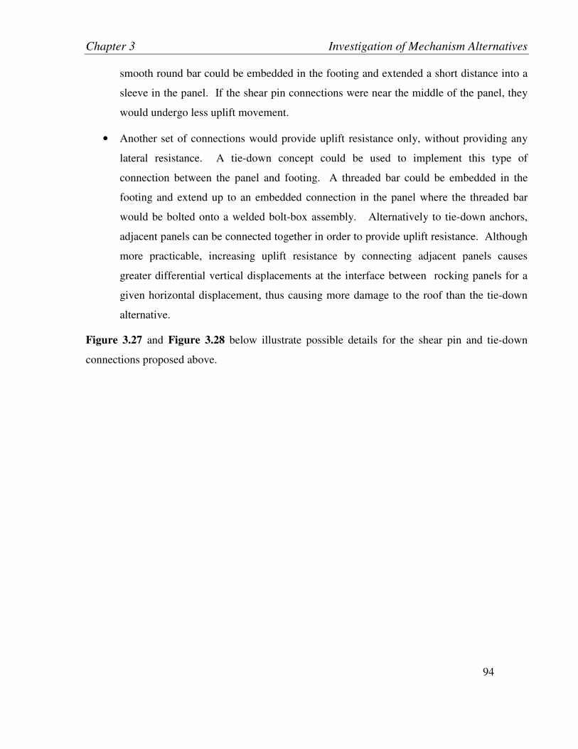
Chapter 3 Investigation of Mechanism Alternatives
94
smooth round bar could be embedded in the footing and extended a short distance into a
sleeve in the panel. If the shear pin connections were near the middle of the panel, they
would undergo less uplift movement.
• Another set of connections would provide uplift resistance only, without providing any
lateral resistance. A tie-down concept could be used to implement this type of
connection between the panel and footing. A threaded bar could be embedded in the
footing and extend up to an embedded connection in the panel where the threaded bar
would be bolted onto a welded bolt-box assembly. Alternatively to tie-down anchors,
adjacent panels can be connected together in order to provide uplift resistance. Although
more practicable, increasing uplift resistance by connecting adjacent panels causes
greater differential vertical displacements at the interface between rocking panels for a
given horizontal displacement, thus causing more damage to the roof than the tie-down
alternative.
Figure 3.27 and Figure 3.28 below illustrate possible details for the shear pin and tie-down
connections proposed above.

Chapter 3 Investigation of Mechanism Alternatives
95
Figure 3.27 Rocking Mechanism – Possible Connection Details: Elevation of Building
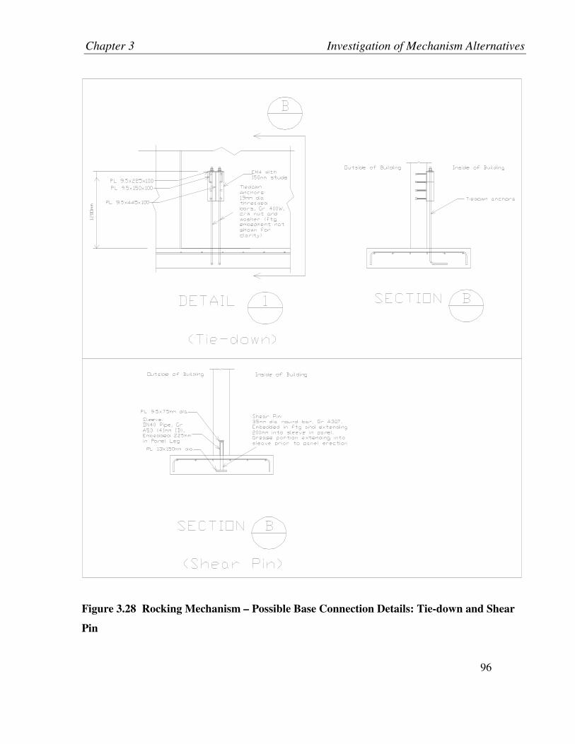
Chapter 3 Investigation of Mechanism Alternatives
96
Figure 3.28 Rocking Mechanism – Possible Base Connection Details: Tie-down and Shear
Pin

Chapter 3 Investigation of Mechanism Alternatives
97
3.7 Incorporating a Rocking Mechanism for Panels with Openings
Considering the greatly increased in-plane strength resulting from connection to adjacent panels,
there is some uncertainty as to whether a frame mechanism could develop for buildings
incorporating panels with large openings similar to Archetype 2. There is limited information on
the panel to slab connections, which may fail prior to a frame mechanism forming, and would
certainly affect the response. Considering this uncertainty, it may be worthwhile to consider
incorporating a rocking mechanism for panels with openings. Results described in Chapter 4 are
utilized, in which a preliminary RdRo value for rocking is assessed to be 2.1. It is important to
note that the assessment of RdRo for the rocking mechanism was done based on a model with 2
adjacent panels connected together and rocking as pairs. This type of arrangement is not
practicable for panels with large openings, since the outside leg of each “rocking pair” of panels
would be required to accommodate the lateral forces transferred from both panels and would
have to be strengthened considerably. Alternatively, the rocking mechanism can be incorporated
for individual panels using the tie-down and shear pin concept as illustrated in Figure 3.27 and
Figure 3.28 above. The RdRo value of 2.1 assessed in Section 4 is still considered valid, since
the tie-down and shear pin concept would provide additional energy dissipation and would likely
increase the assessed RdRo value. Within this section the rocking mechanism is incorporated for
individual panels with openings. Some preliminary sizes of tie-down anchors and shear pins are
provided, based on the details illustrated in Figure 3.28 above and design forces used to
establish Archetype 2.
For Archetype 2, the design in-plane elastic base shear for each leg of each panel was
determined to be 161kN/ leg (refer to Appendix C) based on Rd =1.5 and Ro = 1.3. The
corresponding base shear for RdRo =2.1 would be as follows: (161kN/leg)(1.5)(1.3)/(2.1) = 150
kN/leg. The design of the shear pin is as follows:
1. Material Properties: Round bar conforming to CAN/CSA G40.21, 300W steel, Yield
strength, Fy=300MPa, Ultimate Strength, Fu=450MPa
2. Consider as pin according to CAN/CSA S16-01: Vr = 0.66*øs*Fy*As, where øs=0.9

Chapter 3 Investigation of Mechanism Alternatives
98
3. The required steel area to provide sufficient shear resistance is 840 mm2.
4. A 35mm (1.375”) diameter bar would suffice, with As= 960 mm2.
5. The design shear strength of the bar, Vr = 171kN
6. The nominal shear strength of the bar, Vu = 253 kN (assuming Fu=450MPa and øs=0.9)
7. Concrete embedment would have to be designed accordingly.
The design of the tie-downs is as follows:
1. Material Properties: Round bar conforming to CAN/CSA G30.18, 400W hot-rolled
threaded steel bar, Yield strength, fy=400MPa, assumed ultimate strain, ɛu=0.1
2. Panel Geometry: height = 9.144m, width = 7.62m, weight = 284kN
3. Taking moments about the corner of a panel, the overturning moment is approximately
equal to, Mo = 2*(150kN/leg)*(9.144m height) = 2743 kNm.
4. Tie-down force required at each leg is approximately, T=[(Mo – (284kN)*0.5*7.62m] /
7.62m, so T = 218 kN at each corner of the panel.
5. Consider nominal yield resistance (since preferably this would be the “fuse”), Tr=fy*As,
so the required steel area to provide sufficient force is 545 mm2.
6. 2- 20mm (0.75”) diameter bars would suffice at each corner of the panel, with combined
steel area, As= 600 mm2.
7. A free stressing length of 1200mm would provide uplift displacement capacity of
approximately Duplift = 1200mm*ɛu = 120mm.
8. Hook development length would be required in the footing. Assuming 30MPa concrete
strength, side cover greater than 60mm and end cover greater than 50mm, the hook
development length would be approximately 250mm.
9. EM4 embedded connection with 150mm long studs is required to connect the tie-downs
to the panel. The design shear resistance is 265kN (refer to Figure 1.3), with an
expected ultimate resistance of approximately 440kN.
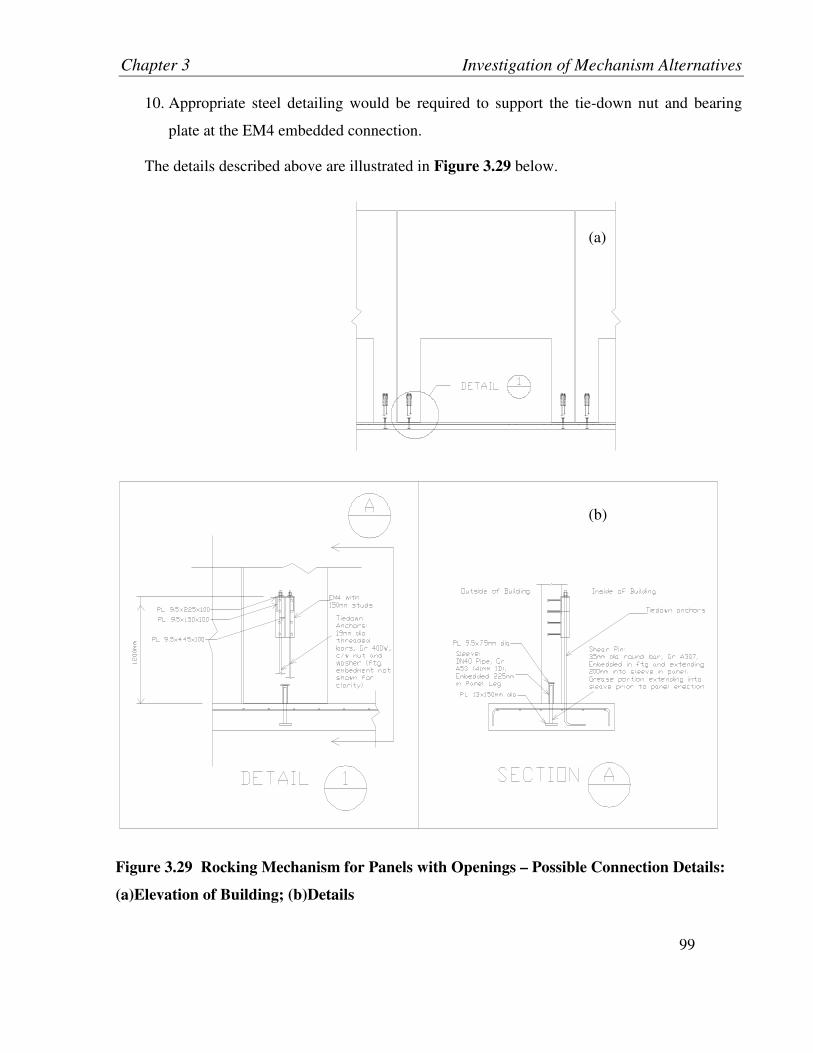
Chapter 3 Investigation of Mechanism Alternatives
99
10. Appropriate steel detailing would be required to support the tie-down nut and bearing
plate at the EM4 embedded connection.
The details described above are illustrated in Figure 3.29 below.
Figure 3.29 Rocking Mechanism for Panels with Openings – Possible Connection Details:
(a)Elevation of Building; (b)Details
(a)
(b)
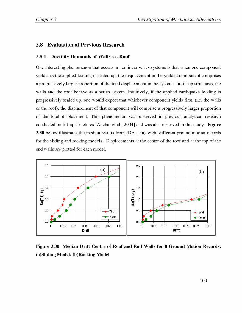
Chapter 3 Investigation of Mechanism Alternatives
100
3.8 Evaluation of Previous Research
3.8.1 Ductility Demands of Walls vs. Roof
One interesting phenomenon that occurs in nonlinear series systems is that when one component
yields, as the applied loading is scaled up, the displacement in the yielded component comprises
a progressively larger proportion of the total displacement in the system. In tilt-up structures, the
walls and the roof behave as a series system. Intuitively, if the applied earthquake loading is
progressively scaled up, one would expect that whichever component yields first, (i.e. the walls
or the roof), the displacement of that component will comprise a progressively larger proportion
of the total displacement. This phenomenon was observed in previous analytical research
conducted on tilt-up structures [Adebar et al., 2004] and was also observed in this study. Figure
3.30 below illustrates the median results from IDA using eight different ground motion records
for the sliding and rocking models. Displacements at the centre of the roof and at the top of the
end walls are plotted for each model.
Figure 3.30 Median Drift Centre of Roof and End Walls for 8 Ground Motion Records:
(a)Sliding Model; (b)Rocking Model
(a) (b)

Chapter 3 Investigation of Mechanism Alternatives
101
As can be observed, the walls yield at approximately Sa(T1) = 0.25g. As the earthquake demand
is scaled up past this yield point, the displacement of the walls comprises a progressively larger
portion of the total displacement. For example, at Sa(T1) = 0.5, results for the sliding model
indicate the walls displace to a drift of 0.003, while the roof displaces to a drift of 0.007, i.e. the
walls take up about 43% of the total displacement. However, at Sa(T1) = 1.5, the walls displace
to a drift of 0.012, while the roof displaces to a drift of 0.016, i.e. the walls take up about 75% of
the total displacement. Similar results can be observed for both the sliding mechanism and the
rocking mechanism (plotted above), as well as for the frame mechanism (not shown).
3.8.2 Ductility Demands on Legs of Frame Panels
One simple method that has been proposed [Adebar et al., 2004] to estimate the inelastic
displacement demands for legs of frame panels is described in the following equation:
)1(*)1(we
wy
dwiV
VTS −=∆
(3.2)
where ∆wi = Inelastic wall displacement
Sd(T) = Spectral displacement at centre of roof
Vwy = Wall strength
Vwe = Maximum elastic demand on walls
The data obtained from the nonlinear dynamic analysis of the frame model for 15 ground
motions was plotted against the above expression to determine how well Equation 3.2 can
predict the displacement demands on the walls (refer to Figure 3.31 below).
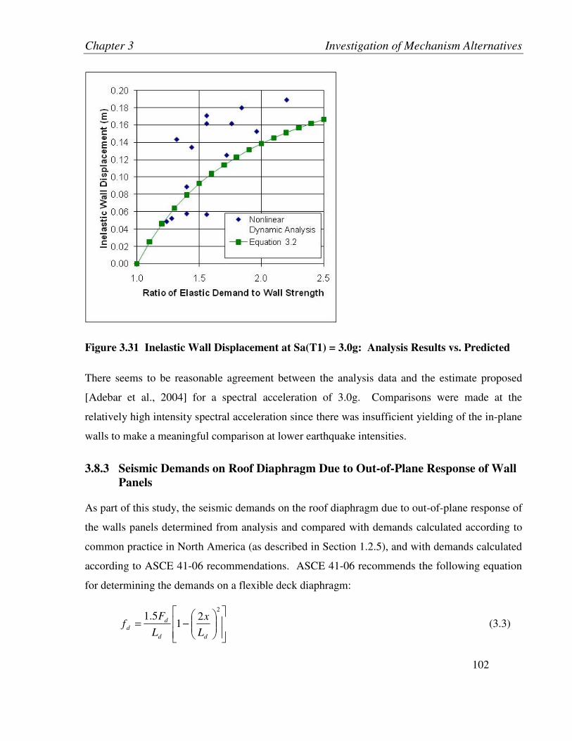
Chapter 3 Investigation of Mechanism Alternatives
102
Figure 3.31 Inelastic Wall Displacement at Sa(T1) = 3.0g: Analysis Results vs. Predicted
There seems to be reasonable agreement between the analysis data and the estimate proposed
[Adebar et al., 2004] for a spectral acceleration of 3.0g. Comparisons were made at the
relatively high intensity spectral acceleration since there was insufficient yielding of the in-plane
walls to make a meaningful comparison at lower earthquake intensities.
3.8.3 Seismic Demands on Roof Diaphragm Due to Out-of-Plane Response of Wall
Panels
As part of this study, the seismic demands on the roof diaphragm due to out-of-plane response of
the walls panels determined from analysis and compared with demands calculated according to
common practice in North America (as described in Section 1.2.5), and with demands calculated
according to ASCE 41-06 recommendations. ASCE 41-06 recommends the following equation
for determining the demands on a flexible deck diaphragm:
−=
22
15.1
dd
d
dL
x
L
Ff
(3.3)

Chapter 3 Investigation of Mechanism Alternatives
103
Where: fd = Inertial load per foot
Fd = Total inertial load on a flexible diaphragm
x = Distance from the center line of flexible diaphragm
Ld = Distance between lateral support points for diaphragm
In plotting Equation 3.3 above, the total inertial load, Fd, was assumed to be the mass of the roof
diaphragm and half the mass of the out-of-plane walls, multiplied by Sa(T1) = 0.5g.
Comparisons were made at a first mode spectral acceleration of 0.5g and are plotted in Figure
3.32 below.
Figure 3.32 Seismic Demands on Roof Diaphragm due to Out-of-Plane Response of Wall
Panels for Sa(T1) = 0.5g: Analysis Results vs. Common North American Practice vs.
ASCE41-06 Approximation

Chapter 3 Investigation of Mechanism Alternatives
104
The plot includes results from analysis of the frame model for all 22 earthquake records
recommended by the ATC-63 Methodology (refer to Table 2.1), scaled to a first mode spectral
acceleration of 0.5g. The results were processed by taking an average of the maximum out-of-
plane connection forces at the top of each roof panel for panels on the long axis of the building.
In all of the models, the walls along the long axis of the building are connected to the roof at four
nodes, as shown in Figure 3.3. At interface locations between panels, the corner node of only
one of the panels is connected to the roof, in order to allow the panels to rock independently of
one another. Due to this eccentricity in the roof-to-panel connections, the connection forces are
not evenly distributed within each panel. Thus it was considered more appropriate to take an
average of the connection forces obtained at the four roof-to-panel connections.
It can be observed within Figure 3.32 that the demands from the median analysis results were
typically higher than demands calculated using common North American practice by up to 50
percent for panels near the middle of the building. It is also apparent that the results were higher
than the ASCE 41-06 parabolic shear load approximation near the ends of the diaphragm.
The most accurate representation of the median analysis results would be obtained by
considering the envelope of forces from the constant shear distribution and the parabolic shear
distribution (i.e. use the constant shear distribution to determine out-of-plane forces near the
ends of the diaphragm and parabolic shear distribution to determine out-of-plane forces near the
middle of the diaphragm). It is noted that there is considerable scatter evident in the results,
particularly toward the high demands.

105
4 QUANTIFICATION OF SEISMIC PERFORMANCE
FACTORS
As discussed in Section 1.2.7, the current methods used for seismic design of tilt-up structures do
not incorporate capacity design principles commonly used in the design of other structural
systems. No clear, stable mechanisms are typically identified for tilt-up systems during design,
and there is considerable uncertainty as to what types of mechanisms would form in many
existing tilt-up structures. In Section 3, several possible mechanisms were identified and
evaluated. Rocking and sliding mechanisms were incorporated into Archetypical System 1; a
frame mechanism was considered for Archetypical System 2. In this section, the rocking
mechanism and the frame mechanism are considered further. In order to incorporate a rocking
mechanism into design, an assessment must be made of an appropriate R-factor. For the frame
mechanism, the current R-factors used for design are based on component testing, without
consideration of the overall response (within this section, R is assumed equivalent to RdRo from
the NBCC 2005.) In order to make a preliminary assessment of an appropriate R-factor for the
rocking mechanism, and to confirm the current R-factors for the frame mechanism, concepts
from the ATC-63 Methodology were used.
4.1 Model 4: Rocking Mechanism
To investigate the response of a building designed to have a failure mechanism characterized by
in-plane rocking of the wall panels, Archetypical System 1 was considered but the connection
layout was modified. Two adjacent panels were connected together at the end walls (in-plane
walls along the short axis of the building), such that two sets of two adjacent panels could rock
independently at end walls. Each set of two panels was assumed to have connections at the base
that would stop sliding from occurring but would allow rocking (refer to shear pin connection in
Figure 3.28.) In addition, connections at corners were removed such that panels could rock
independently in different directions. Figure 4.1 below illustrates the assumed connection
layout. The sections shown in the figure are referenced from Figure 2.4.

Chapter 4 Quantification of Seismic Performance Factors
106
Figure 4.1 Rocking Model – 2 Adjacent Panels Connected at End Walls
The model is similar to the one used to make comparisons between the different mechanisms
(refer to Section 1 for details). The only difference being the additional connections between the
end wall panels. The change in the model was verified to ensure reasonable behaviour by
conducting a pushover analysis in the direction of the short axis of the building and comparing
the results to hand calculations. Figure 4.2 below illustrates the results of this analysis.

Chapter 4 Quantification of Seismic Performance Factors
107
Figure 4.2 Rocking Model - Pushover Analysis Along Short Axis of Building (2 panels
connected)
The results indicate good agreement between the Perform and hand calculations. The yield
strength of this model is 0.3W, where W is the seismic weight of the building. The NBCC 2005
elastic design base shear based on the first mode period calculated according to the code formula
and Site Class D in Vancouver is 0.68W. The NBCC 2005 design base shear used incorporates
the two-thirds cut-off rule since it was also incorporated in design of the building archetypes. If
the ASCE 41 formula (Equation 3.1) is used to determine the fundamental period, the elastic
design base shear for a Site Class D building in Vancouver would be 0.64W. This effectively
means the design of the in-plane walls is based on an RdRo value of 2.3. It is important to note
that R-values are structure specific and not location specific. The assessment in this study uses
the Vancouver design base shear to evaluate whether an RdRo value of 2.3 is adequate for a
rocking model. Vancouver was selected as the location since it has a relatively high design base
Chapter 4 Quantification of Seismic Performance Factors
108
shear. If it is established that this RdRo value is adequate for the Vancouver design base shear, it
should be reasonable to use this RdRo value for other design base shear values.
4.1.1 Simulated and Non-Simulated Collapse
The rocking of the walls is the only mechanism that is simulated in the modeling. Non-
simulated collapse mechanisms include yielding of the roof diaphragm, rupture of the out-of-
plane wall to roof connectors, and excessive deformation of the gravity columns. Non-simulated
collapse mechanisms were evaluated by tracking the forces and deformations associated with the
mechanisms and comparing with calculated capacities.
The roof diaphragm was designed based on SDI provisions with recommended safety factors.
The nominal strength of the roof diaphragm was evaluated based on removing SDI safety factors
and considering results from recent testing [Hilti, 2008]. The nominal strength for the decking
arrangement used in Zone 2 (refer to Figure 2.5) was determined to be 70 kN/m, compared to a
factored design strength of 31 kN/m. Refer to Appendix B for detailed calculations.
The nominal capacity of the out-of-plane wall to roof connections was determined by
considering NBCC 2005 design forces and removing safety factors from design capacities of
connectors. It was assumed that designers would typically provide sufficient connections and
drag struts into the deck to transfer the NBCC 2005 design out-of-plane forces. The factored
resistance of out-of-plane wall to roof connections was determined based on testing (Lemieux et.
al, 1998). The average nominal strength determined from the test results was multiplied by 0.6
to obtain the factored design strengths shown in the Concrete Design Handbook (CAC 2006) and
illustrated in Figure 1.3. In removing this safety factor, the nominal strength of the out-of-plane
connections was estimated to be 42 kN/m, compared to a design capacity of 25 kN/m.
Allowable lateral deflections for the gravity columns was determined by considering the
interaction between the unfactored design axial load and the second order moment that occurs in
the gravity columns when the roof is displaced. The maximum allowable roof drift before the
gravity columns could no longer adequately support the unfactored design axial load was
estimated to be 0.03. A maximum allowable drift of 0.03 was considered appropriate, since the
NBCC 2005 requires that the interstory drift for a structure must be limited to 0.025. It is
Chapter 4 Quantification of Seismic Performance Factors
109
recognized that the assessment of the gravity columns was based only on force capacities and
that deformations at collapse may be much larger.
Within this study, the primary acceptance criteria used to determine the suitability of a selected
R value was the criteria for a maximum roof drift of 0.03. The other criteria for non-simulated
collapse, including in-plane yielding of the roof deck diaphragm and failure of the out-of-plane
panel to roof connectors were monitored in order to determine if higher design strengths would
be required in order to ensure the roof drift criteria could be met.
4.1.2 IDA Results, Collapse Statistics and Uncertainty
Incremental dynamic analysis was carried out for the 22 ground motion record pairs
recommended by the ATC-63 Methodology (Table 2.1). Each record pair was applied
simultaneously to the model, in orthogonal directions. The IDA results are shown plotted in
Figure 4.3 below.

Chapter 4 Quantification of Seismic Performance Factors
110
Figure 4.3 Rocking Model – IDA Results for 22 Ground Motion Record Pairs: (a)Drift at
End Wall; (b)Drift at Centre of Roof; (c)In-Plane Deck Forces at End Walls; (d)Out-of-
Plane Wall to Roof Connection Forces
It is interesting to note that as the end walls yield the slope of the IDA curve for the in-plane
deck forces in Figure 4.3c increases, indicating the forces imparted to the deck is limited by the
rocking of the walls. This confirms previous research (Adebar et al., 2004) that indicated that in
(a) (b)
(d) (c)
Chapter 4 Quantification of Seismic Performance Factors
111
a series system, when one component yields, it shields the other components from greater forces.
The collapse data for the model is established for each non-simulated collapse mechanism by
considering the first mode spectral acceleration at which the IDA curve for each individual
earthquake record exceeds the collapse threshold. The median value from the collapse data is
then used to define a lognormal cumulative distribution to describe the collapse statistics for
each non-simulated collapse mechanism. Refer to Appendix D for sample calculations on how
the collapse statistics are determined.
As discussed in Section 2.6, the ATC-63 Methodology requires consideration of variability due
to modeling uncertainties, uncertainty in how representative the archetype design is to actual
structures (termed “design requirements”), and uncertainty relating to the amount of test data.
Values of variability are assigned to each of these uncertainties and are used to establish an
aggregate variability for each non-simulated collapse mechanism. This aggregate variability is
then incorporated into the lognormal distribution used to fit the collapse data, in order to adjust
the curve. An increase in the degree of uncertainty judged to be in the analysis causes a
corresponding increase in the amount of adjustment that is applied to the lognormal distribution,
resulting in a more conservative distribution. For the rocking model, the following values were
adopted:
• Record to record uncertainties, βRTR= 0.37 for the non-simulated collapse due to drift,
0.36 for in-plane deck forces, and 0.47 for out-of-plane deck forces.
(This value was calculated directly from the collapse data for each non-simulated
collapse mode, and is equal to the standard deviation of the natural log of the collapse
spectral acceleration results)
• Modeling uncertainties, βMDL=0.45 was selected. The model was judged to be a “fair”
representation of the actual structure. The reason for the relatively high uncertainty
assigned to modeling is that the model does not incorporate the non-linear response of
the roof deck diaphragm. Also, for the frame and eccentric models, there is no
consideration of the behaviour of the panel to slab connections.
• Design requirements, βDR=0.3 was selected. As a result of the survey conducted (refer to
Table 2.2) with various tilt-up contractors and consultants in the US and Canada, there is
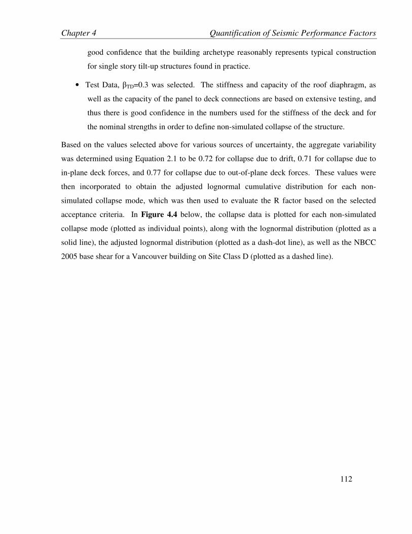
Chapter 4 Quantification of Seismic Performance Factors
112
good confidence that the building archetype reasonably represents typical construction
for single story tilt-up structures found in practice.
• Test Data, βTD=0.3 was selected. The stiffness and capacity of the roof diaphragm, as
well as the capacity of the panel to deck connections are based on extensive testing, and
thus there is good confidence in the numbers used for the stiffness of the deck and for
the nominal strengths in order to define non-simulated collapse of the structure.
Based on the values selected above for various sources of uncertainty, the aggregate variability
was determined using Equation 2.1 to be 0.72 for collapse due to drift, 0.71 for collapse due to
in-plane deck forces, and 0.77 for collapse due to out-of-plane deck forces. These values were
then incorporated to obtain the adjusted lognormal cumulative distribution for each non-
simulated collapse mode, which was then used to evaluate the R factor based on the selected
acceptance criteria. In Figure 4.4 below, the collapse data is plotted for each non-simulated
collapse mode (plotted as individual points), along with the lognormal distribution (plotted as a
solid line), the adjusted lognormal distribution (plotted as a dash-dot line), as well as the NBCC
2005 base shear for a Vancouver building on Site Class D (plotted as a dashed line).

Chapter 4 Quantification of Seismic Performance Factors
113
Figure 4.4 Rocking Model – Collapse Statistics: (a)Roof Drift; (b)In-Plane Deck Forces;
(c)Out-of-Plane Deck Forces
As can be observed in Figure 4.4 above, for all three non-simulated collapse modes considered,
the lognormal distribution fits the collapse data reasonably well. The collapse data for the out-
of-plane deck force collapse mode exhibits some scatter at the tail of the distribution.
4.1.3 Acceptance Criteria and Evaluation of R
As discussed previously in Section 2.8, for the purposes of this study, a maximum probability of
collapse of 0.1 is adopted for the design earthquake with an annual excedence frequency of 1 in
(a)
(c)
(b)

Chapter 4 Quantification of Seismic Performance Factors
114
2475. For the roof drift failure mode, using the adjusted cumulative distribution shown as the
dash-dot line in Figure 4.4 (a), it was determined that there was a 10% probability of exceeding
a roof drift of 3% at Sa(T1)=0.62g. The 2005 NBCC design base shear for the in-plane walls is
0.68W, corresponding to a 12% probability of exceeding the selected drift limit of 3%. This
does not meet the acceptance criteria adopted for this study, and thus the design of the in-plane
walls is not adequate. The RdRo value of 2.3 which was initially assumed would have to be
reduced in order to effectively increase the acceleration corresponding to a 10% probability of
exceeding the 3% drift criteria. If linear interpolation is used to determine the reduced RdRo
value, the new value would be approximately equal to (2.3)(0.62g)/(0.68g) = 2.1. Note that the
adjustment for spectral shape is not included in this assessment.
It is interesting to note that if the first mode period determined from analysis and based on
Equation 3.1 is used instead of the NBCC 2005 code formula, the design base shear reduces to
0.64g, which is very similar to the spectral acceleration corresponding to a 10% probability of
exceeding the 3% drift criteria. If this base shear was used for design, the effective RdRo value
would be 2.1.
Based on the above, an RdRo value of 2.1 for design of the in-plane walls using a rocking
mechanism would meet the acceptance criteria adopted for this study. It should be noted that the
means to provide the strength required to achieve the target RdRo value does not need to be by
connection of adjacent panels. A rocking mechanism could also be achieved by other means,
including using connections similar to those proposed in Section 3.6.
To determine the adequacy of the roof deck for in-plane forces, the median spectral acceleration
at which the deck would yield was determined based on data used for Figure 4.3 (c) to be 1.4g.
Using the adjusted cumulative distribution for in-plane forces shown in Figure 4.4 (b), the
spectral acceleration corresponding to a 10% probability of exceeding the in-plane strength of
the roof deck was determined to be 0.55g. Since the design base shear used for design of the
roof deck diaphragm was 0.68g, the design of the roof deck for in-plane forces does not meet the
acceptance criteria adopted within this study. In order to meet the acceptance criteria, the
strength of the roof for in-plane forces would have to be increased by approximately 25%.

Chapter 4 Quantification of Seismic Performance Factors
115
A similar procedure was carried out to determine the adequacy of the out-of-plane panel to roof
connections. The median first mode spectral acceleration at which the connections would fail
was determined based on data used for Figure 4.3 (d) to be 0.98g. Using the adjusted lognormal
cumulative distribution shown in Figure 4.4 (c), the first mode spectral acceleration
corresponding to a 10% probability of exceeding the nominal strength of the out-of-plane panel
to roof connections was determined to be 0.39g.
The demands on the out-of-plane wall to roof connections calculated according to the NBCC
2005 depend partly on the first mode spectral acceleration of the building and partly on the
flexibility of the component being considered (refer to Section 1.2.3). However as a means of
comparison with the IDA plots for the overall structure, the design base shear for the building
was used (0.68g). As such, the design of the out-of-plane wall to roof connections does not meet
the acceptance criteria adopted within this study. In order to meet the acceptance criteria, the
strength of the wall to roof connections for out-of-plane forces would have to be increased by
approximately 90%.
To summarize, an RdRo value of 2.1 is probably reasonable for the rocking mechanism for this
building archetype, though the in-plane diaphragm resistance would have to be increased by 25%
and the wall-to-roof connections for out-of-plane loading would have to be increased by
approximately 90%.
4.2 Model 5: Frame Mechanism
To investigate the response of a building designed to have a failure mechanism characterized by
in-plane yielding of the legs of wall panels with large openings, Archetypical System 2 was
considered. The model used to carry out the analyses is identical to the model used to make
comparisons between different mechanisms. Refer to Section 3.4.3 for details.
The NBCC 2005 design base shear based on the first mode period calculated according to the
code formula and Site Class D is 0.68g. For design, the legs for the in-plane walls with large
openings were designed based on an Rd = 1.5 and Ro = 1.3, resulting in a combined RdRo value
of 1.95. Due to the connections between adjacent panels, the legs of the adjacent end wall panels
with large openings behave essentially as a single unit, resulting in much higher in-plane

Chapter 4 Quantification of Seismic Performance Factors
116
strengths (refer to Figure 3.14). Consequently, the yield strength of this model in the direction
of the short axis of the building is 0.87g. This effectively means the design of the in-plane walls
is based on an RdRo value less than 1.
4.2.1 Simulated and Non-Simulated Collapse
In-plane flexural yielding of legs of wall panels with large openings is the primary mechanism
that is simulated in the modeling. Shear failure is also modelled explicitly. Non-simulated
collapse mechanisms include yielding of the roof diaphragm, rupture of the out-of-plane wall to
roof connectors, and excessive deformation of the gravity columns. Non-simulated collapse
mechanisms were evaluated by tracking the forces and deformations associated with the
mechanisms and comparing with calculated capacities. Refer to Section 4.1.1 for a discussion
on the non-simulated collapse mechanisms considered and their nominal capacities.
4.2.2 IDA Results, Collapse Statistics and Uncertainty
Incremental dynamic analysis was carried out for the 22 ground motion record pairs
recommended by the ATC-63 Methodology (Table 2.1). Each record pair was applied
simultaneously to the model, in orthogonal directions. The IDA results are shown plotted in
Figure 4.5 below.
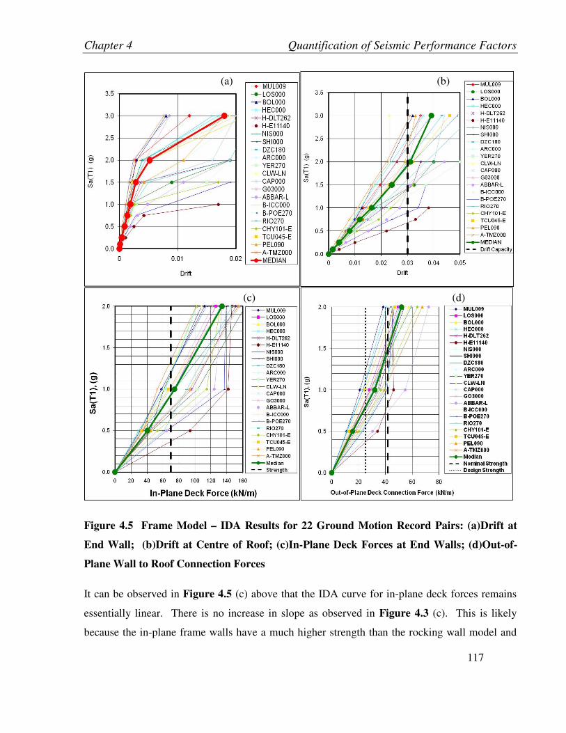
Chapter 4 Quantification of Seismic Performance Factors
117
Figure 4.5 Frame Model – IDA Results for 22 Ground Motion Record Pairs: (a)Drift at
End Wall; (b)Drift at Centre of Roof; (c)In-Plane Deck Forces at End Walls; (d)Out-of-
Plane Wall to Roof Connection Forces
It can be observed in Figure 4.5 (c) above that the IDA curve for in-plane deck forces remains
essentially linear. There is no increase in slope as observed in Figure 4.3 (c). This is likely
because the in-plane frame walls have a much higher strength than the rocking wall model and
(a) (b)
(d) (c)
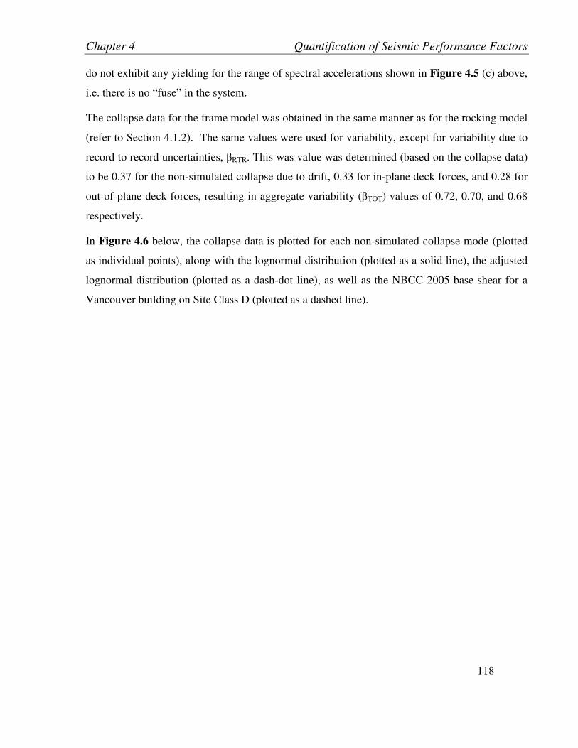
Chapter 4 Quantification of Seismic Performance Factors
118
do not exhibit any yielding for the range of spectral accelerations shown in Figure 4.5 (c) above,
i.e. there is no “fuse” in the system.
The collapse data for the frame model was obtained in the same manner as for the rocking model
(refer to Section 4.1.2). The same values were used for variability, except for variability due to
record to record uncertainties, βRTR. This was value was determined (based on the collapse data)
to be 0.37 for the non-simulated collapse due to drift, 0.33 for in-plane deck forces, and 0.28 for
out-of-plane deck forces, resulting in aggregate variability (βTOT) values of 0.72, 0.70, and 0.68
respectively.
In Figure 4.6 below, the collapse data is plotted for each non-simulated collapse mode (plotted
as individual points), along with the lognormal distribution (plotted as a solid line), the adjusted
lognormal distribution (plotted as a dash-dot line), as well as the NBCC 2005 base shear for a
Vancouver building on Site Class D (plotted as a dashed line).
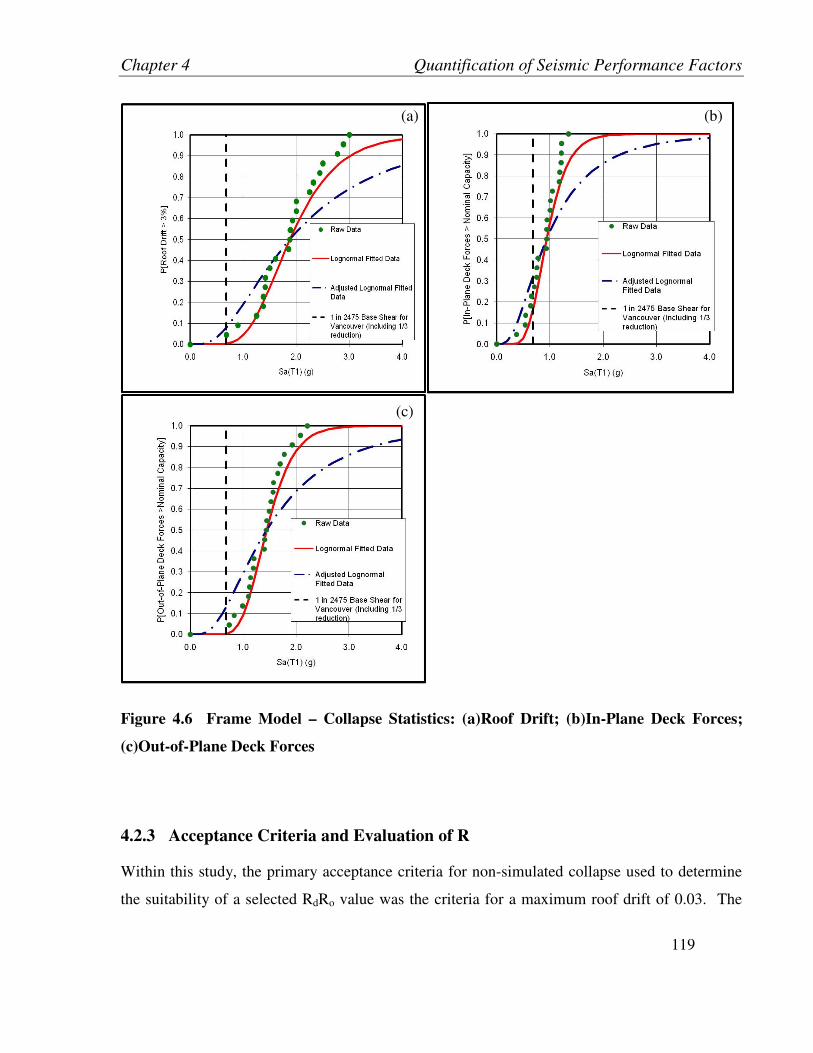
Chapter 4 Quantification of Seismic Performance Factors
119
Figure 4.6 Frame Model – Collapse Statistics: (a)Roof Drift; (b)In-Plane Deck Forces;
(c)Out-of-Plane Deck Forces
4.2.3 Acceptance Criteria and Evaluation of R
Within this study, the primary acceptance criteria for non-simulated collapse used to determine
the suitability of a selected RdRo value was the criteria for a maximum roof drift of 0.03. The
(a)
(c)
(b)
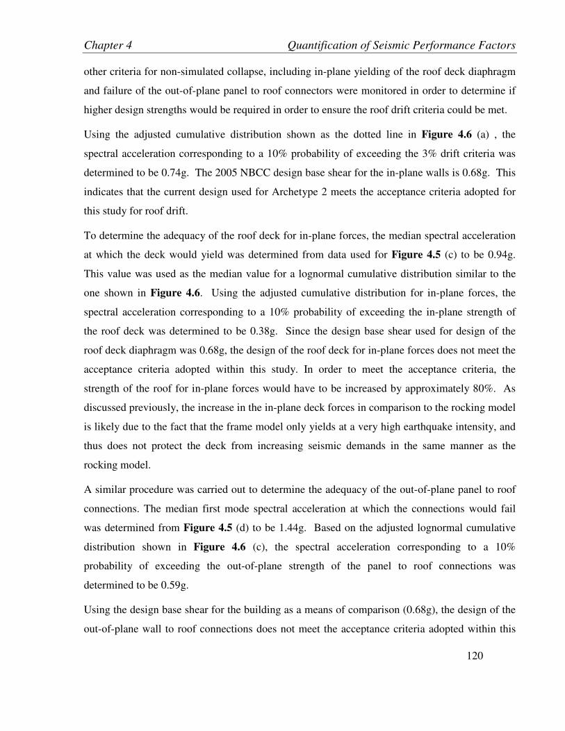
Chapter 4 Quantification of Seismic Performance Factors
120
other criteria for non-simulated collapse, including in-plane yielding of the roof deck diaphragm
and failure of the out-of-plane panel to roof connectors were monitored in order to determine if
higher design strengths would be required in order to ensure the roof drift criteria could be met.
Using the adjusted cumulative distribution shown as the dotted line in Figure 4.6 (a) , the
spectral acceleration corresponding to a 10% probability of exceeding the 3% drift criteria was
determined to be 0.74g. The 2005 NBCC design base shear for the in-plane walls is 0.68g. This
indicates that the current design used for Archetype 2 meets the acceptance criteria adopted for
this study for roof drift.
To determine the adequacy of the roof deck for in-plane forces, the median spectral acceleration
at which the deck would yield was determined from data used for Figure 4.5 (c) to be 0.94g.
This value was used as the median value for a lognormal cumulative distribution similar to the
one shown in Figure 4.6. Using the adjusted cumulative distribution for in-plane forces, the
spectral acceleration corresponding to a 10% probability of exceeding the in-plane strength of
the roof deck was determined to be 0.38g. Since the design base shear used for design of the
roof deck diaphragm was 0.68g, the design of the roof deck for in-plane forces does not meet the
acceptance criteria adopted within this study. In order to meet the acceptance criteria, the
strength of the roof for in-plane forces would have to be increased by approximately 80%. As
discussed previously, the increase in the in-plane deck forces in comparison to the rocking model
is likely due to the fact that the frame model only yields at a very high earthquake intensity, and
thus does not protect the deck from increasing seismic demands in the same manner as the
rocking model.
A similar procedure was carried out to determine the adequacy of the out-of-plane panel to roof
connections. The median first mode spectral acceleration at which the connections would fail
was determined from Figure 4.5 (d) to be 1.44g. Based on the adjusted lognormal cumulative
distribution shown in Figure 4.6 (c), the spectral acceleration corresponding to a 10%
probability of exceeding the out-of-plane strength of the panel to roof connections was
determined to be 0.59g.
Using the design base shear for the building as a means of comparison (0.68g), the design of the
out-of-plane wall to roof connections does not meet the acceptance criteria adopted within this

Chapter 4 Quantification of Seismic Performance Factors
121
study. The strength of the connections would have to be increased by approximately 15% to
meet the acceptance criteria. This indicates that the response of the frame model resulted in
lower out-of-plane forces on the panel to roof connections than the rocking model. Considering
that the in-plane deck forces increased considerably, this result may seem counter-intuitive.
However, two aspects must be considered:
• In the NBCC 2005 Clause 4.1.8.17 regarding seismic demands on elements of structures,
non-structural components and equipment, the more flexible a component is, the higher
the amplification value, Ar, ascribed to it (refer to Section 1.2.1). Since the panels are
essentially components of the building, it is reasonable that the less flexible frame model
results in lower out-of-plane panel to deck forces than the more flexible rocking model.
• The panels often do not oscillate in phase in the out-of-plane direction. In many
instances, some panels are flexing in one direction while others are flexing in the
opposite direction. This is due to the difference in the roof stiffness (essentially the out-
of-plane lateral support for the wall panel) between the edges of the building and the
middle of the building. Thus it is reasonable that even though the out-of-plane forces
may be higher, this may not result in higher in-plane forces overall.
In summary, the current RdRo values used with a connection layout commonly used in practice
yield results that are within the acceptance criteria adopted within this study for maximum roof
drift. With the current design, the in-plane diaphragm resistance would have to be increased by
80% and the wall-to-roof connections for out-of-plane loading would have to be increased by
approximately 15%.
4.3 Model 6: Frame Mechanism – Eccentric Building
To investigate the response of a building with large openings on one side and solid panels on the
other, Archetypical System 2 was modified by incorporating solid panels at one end wall.
The model used to carry out the analyses is similar to Model 3 used to make comparisons
between different mechanisms, except that solid panels were incorporated at one end wall that
were rigidly connected to each other and at the base. Refer to Section 3.4.3 for details on Model
3.

Chapter 4 Quantification of Seismic Performance Factors
122
The NBCC 2005 design base shear based on the first mode period calculated according to the
code formula and Site Class D is 0.68g. For design, the legs for the in-plane walls with large
openings were designed based on an Rd = 1.5 and Ro = 1.3, resulting in a combined RdRo value
of 1.95. Due to the connections between adjacent panels, the legs of the adjacent end wall panels
with large openings behave essentially as a single unit, resulting in much higher in-plane
strengths (refer to Figure 3.13 and Figure 3.14).
4.3.1 Simulated and Non-Simulated Collapse
In-plane flexural yielding of the wall panels with large openings is the primary mechanism that
is simulated in the modeling. Non-simulated collapse mechanisms include yielding of the roof
diaphragm, rupture of the out-of-plane wall to roof connectors, and excessive deformation of the
gravity columns. Non-simulated collapse mechanisms were evaluated by tracking the forces and
deformations associated with the mechanisms and comparing with calculated capacities. Refer
to Section 4.1.1 for a discussion on the non-simulated collapse mechanisms considered and their
nominal capacities.
4.3.2 IDA Results, Collapse Statistics and Uncertainty
Incremental dynamic analysis was carried out for the 22 ground motion record pairs
recommended by the ATC-63 Methodology (Table 2.1). Each record pair was applied
simultaneously to the model, in orthogonal directions. The IDA results for roof drift are shown
plotted in Figure 4.7 below.
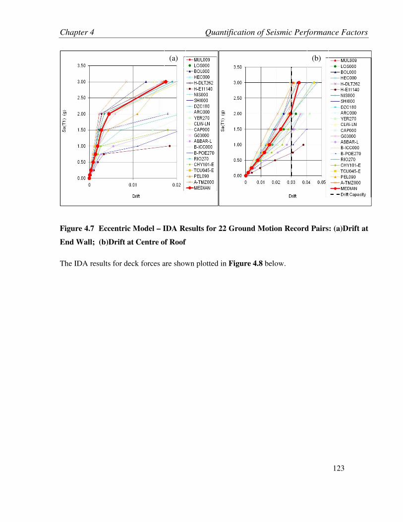
Chapter 4 Quantification of Seismic Performance Factors
123
Figure 4.7 Eccentric Model – IDA Results for 22 Ground Motion Record Pairs: (a)Drift at
End Wall; (b)Drift at Centre of Roof
The IDA results for deck forces are shown plotted in Figure 4.8 below.
(a) (b)
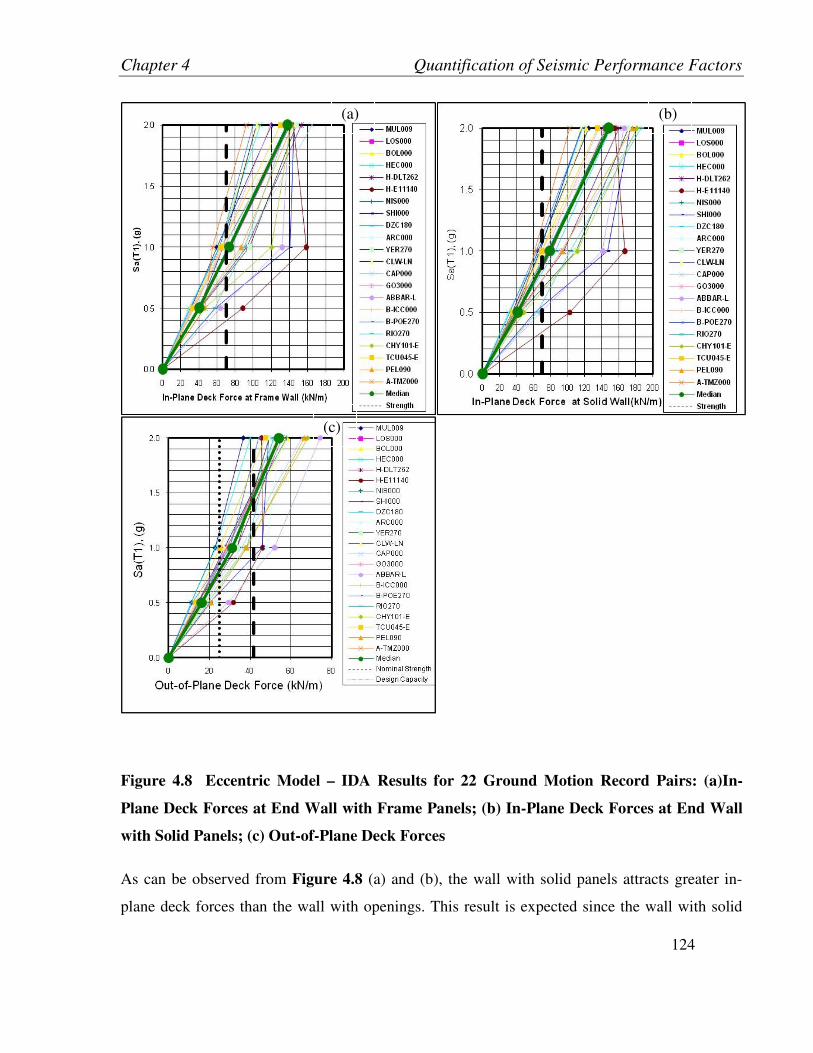
Chapter 4 Quantification of Seismic Performance Factors
124
Figure 4.8 Eccentric Model – IDA Results for 22 Ground Motion Record Pairs: (a)In-
Plane Deck Forces at End Wall with Frame Panels; (b) In-Plane Deck Forces at End Wall
with Solid Panels; (c) Out-of-Plane Deck Forces
As can be observed from Figure 4.8 (a) and (b), the wall with solid panels attracts greater in-
plane deck forces than the wall with openings. This result is expected since the wall with solid
(a) (b)
(c)
Chapter 4 Quantification of Seismic Performance Factors
125
panels does not yield and is much stiffer. The in-plane deck forces at the end wall with solid
panels will be considered in this assessment.
The collapse data for the frame model was obtained in the same manner as for the rocking model
(refer to Section 4.1.2). The same values were used for variability, except for variability due to
record to record uncertainties, βRTR. This was value was determined (based on the collapse data)
to be 0.36 for the non-simulated collapse due to drift, 0.31 for in-plane deck forces, and 0.29 for
out-of-plane deck forces, resulting in aggregate variability (βTOT) values of 0.72, 0.69, and 0.68
respectively.
In Figure 4.9 below, the collapse data is plotted for each non-simulated collapse mode (plotted
as individual points), along with the lognormal distribution (plotted as a solid line), the adjusted
lognormal distribution (plotted as a dash-dot line), as well as the NBCC 2005 base shear for a
Vancouver building on Site Class D (plotted as a dashed line).
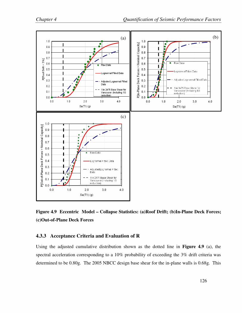
Chapter 4 Quantification of Seismic Performance Factors
126
4.3.3 Acceptance Criteria and Evaluation of R
Using the adjusted cumulative distribution shown as the dotted line in Figure 4.9 (a), the
spectral acceleration corresponding to a 10% probability of exceeding the 3% drift criteria was
determined to be 0.80g. The 2005 NBCC design base shear for the in-plane walls is 0.68g. This
Figure 4.9 Eccentric Model – Collapse Statistics: (a)Roof Drift; (b)In-Plane Deck Forces;
(c)Out-of-Plane Deck Forces
(a)
(c)
(b)
Chapter 4 Quantification of Seismic Performance Factors
127
indicates that the current design used for Archetype 2 meets the acceptance criteria adopted for
this study for roof drift, even if the building is significantly eccentric.
To determine the adequacy of the roof deck for in-plane forces, the median spectral acceleration
at which the deck would yield near the end wall with solid wall panels was determined from data
used for Figure 4.8 (b) to be 0.85g. Using the adjusted cumulative distribution for in-plane
forces (refer to Figure 4.9 (b)), the spectral acceleration corresponding to a 10% probability of
exceeding the in-plane strength of the roof deck was determined to be 0.35g. Since the design
base shear used for design of the roof deck diaphragm was 0.68g, the design of the roof deck for
in-plane forces does not meet the acceptance criteria adopted within this study. In order to meet
the acceptance criteria, the strength of the roof for in-plane forces would have to be increased by
approximately 95%.
The median first mode spectral acceleration at which the out-of-plane panel to roof connections
would fail was determined from data used for Figure 4.8 (c) to be 1.47g. Based on the adjusted
lognormal cumulative distribution shown in Figure 4.9 (c), the spectral acceleration
corresponding to a 10% probability of exceeding the in-plane strength of the roof deck was
determined to be 0.61g.
Using the design base shear for the building as a means of comparison (0.68g), the design of the
out-of-plane wall to roof connections does not meet the acceptance criteria adopted within this
study. The strength of the connections would have to be increased by approximately 10% to
meet the acceptance criteria.
To summarize, the current RdRo values used with a connection layout commonly used in practice
lead to results that are within the acceptance criteria adopted within this study for maximum roof
drift. With the current design, the in-plane diaphragm resistance would have to be increased by
95% and the wall-to-roof connections for out-of-plane loading would have to be increased by
approximately 10%.
4.3.4 Comparison of IDA Results from Rocking, Frame and Eccentric Models
Figure 4.10 below compares median IDA results for the rocking, frame, and eccentric models.

Chapter 4 Quantification of Seismic Performance Factors
128
Figure 4.10 Comparison of IDA Results for the Rocking Model, Frame Model, and
Eccentric Model: (a)Drift at End Walls with Openings; (b)Drift at Centre of Roof (c)In-
Plane Deck Forces; (d) Out-of-Plane Deck Forces
There was not much difference in the results for the wall drift between the frame building and
the eccentric frame building. This is likely due to the greatly increased stiffness and strength of
(a) (b)
(d) (c)
Chapter 4 Quantification of Seismic Performance Factors
129
the frame panels resulting from the connection of adjacent frame panels together. The walls did
not experience considerable yielding until very high earthquake intensities were applied. Also,
due to the connection layout between adjacent panels, there was limited non-linear response,
since ultimate strains in the rebar were attained quickly once yielding occurred.
It is interesting to note the differences in the roof responses between the different models. The
roof displacement for the eccentric model is less than that for the frame model. This is thought
to occur because the eccentric building has one end wall that maintains stiffness as the frame
panel’s yield, thus reducing displacements at the centre of the roof. It is evident in Figure 4.10
(c) that the end wall with solid panels attracts more load (higher in-plane deck forces) than the
end wall with frame panels. As expected, the in-plane deck forces for the rocking model are
significantly less than for the frame and eccentric models, due to the lower yield base shear
exhibited by the rocking model.
There are also differences in the out-of-plane wall to roof connection forces for the different
models. The rocking model experiences higher out-of-plane wall to roof connection forces than
the other two models, though the in-plane forces decrease. The rationale for these observations
is discussed previously in Section 4.2.3. This result suggests that an increase in the end wall
strength results in lower out-of-plane wall to roof connection forces.
130
5 CONCLUSIONS AND RECOMMENDATIONS
The research discussed within this report consists of an analytical study to investigate the seismic
performance of single-story tilt-up structures with steel deck roof diaphragms. Within this
section, a summary of observations from this study is provided and recommendations are
included.
5.1 Summary of Observations
A review of current practice in North America for the seismic design of tilt-up structures
revealed the following points of interest:
• The calculation of the fundamental building period for determination of the design base
shear does not include any consideration of the flexibility of the roof diaphragm, but
instead is based solely on the height of the concrete wall panels.
• Design for seismic loading is carried out using a strictly force-based approach. Sufficient
panel to roof, panel to panel and panel to slab connections are provided to accommodate
the design forces, but there is no explicit consideration of a stable energy-dissipation
mechanism that would be expected to occur upon failure of the connections. This is
inconsistent with capacity-design approaches used in current practice for seismic design
of other building systems, such as moment frames, braced frames, and shear walls.
Some possible energy-dissipation mechanisms for tilt-up structures were investigated and
compared, including rocking of wall panels, sliding of wall panels, and frame action for
buildings with wall panels incorporating large openings. In comparing rocking and sliding
mechanisms, it was determined that although the sliding mechanism provides significantly more
energy dissipation, and hence lower drift demands, it would be very difficult to incorporate
sliding into common applications. Many tilt-up buildings are not perfectly rectangular; re-
entrant corners are often required to accommodate a certain building layout, also some walls
may not be parallel to one another. In addition, it would be difficult to consistently estimate the
Chapter 5 Conclusions and Recommendations
131
sliding resistance of a panel since it depends on the friction between the panel and footing, which
is expected to vary. Also, sliding results in permanent deformation of the wall panels, which is
undesirable. The rocking mechanism would not result in any permanent deformation of the wall
panels, but would likely cause damage to the roof perimeter angle used to transfer shear and
axial loads from the roof diaphragm to the tilt-up walls. Damage is expected due to differential
vertical movement at the interface between adjacent panels. One possible way to mitigate this
problem would be to stop the roof perimeter angle at the embedded connectors in the wall panels
nearest the panel to panel interface and provide a pin ended connector angle between panels.
Investigation of the frame mechanism was carried out by considering a tilt-up building
incorporating panels with large openings, with sufficient connections provided to resist design
forces. It was found that connections between adjacent panels provided sufficient shear transfer
between panels to result in legs of adjacent panels effectively acting as a single member. For
panels with openings, this led to flexural strengths double the design values, and in turn, higher
in-plane base shear resistance for the overall building. However, the connection of legs also
resulted in lower deformation capacity of the legs, leading to a potentially undesirable brittle
failure mode. One limitation in the modeling of the frame mechanism was that the panel to slab
connections were modeled as a pinned base due to lack of information on the slab to wall
connector (Devine 2009).
Results from nonlinear analysis using building models prepared for this study were used to
evaluate findings from previous research on tilt-up buildings. The key findings are as follows:
• The fundamental period determined from the Perform 3D building model was compared
to the formula recommended by ASCE 41-06 (refer to Equation 3.1). The ASCE 41-06
equation takes into consideration wall and roof displacements resulting from a uniformly
distributed lateral load equal to the weight of the roof diaphragm. It was determined that
if the equation was modified by adding half the weight of the out-of-plane walls to the
lateral load used to calculate wall and roof displacements, there was a good match
between the ASCE 41-06 equation and the first mode period determined from Perfrom
3D (within 10%).

Chapter 5 Conclusions and Recommendations
132
• In previous analytical research (Adebar et al., 2004) tilt-up structures were modelled as a
two component series system, one component representing the walls while the other
represents the roof. Adebar et al. observed that if one component in the system yields,
the displacement of the yielding component comprises a progressively larger portion of
the total displacement as the intensity of the applied loading is increased. This
behaviour was also observed in the current study.
• In previous analytical research on tilt-up structures with large openings (Adebar et al.,
2004), an expression to estimate the inelastic displacement demands for legs of frame
panels was proposed (Equation 3.2). This expression was plotted against data from the
current study and was found to fit the data reasonably well. However, further study
should be carried out with alternative arrangements / models to provide further
verification for this expression.
• For design, seismic loads on the roof diaphragm are typically assumed to have a uniform
distribution. ASCE 41-06 recommends a parabolic seismic load distribution for flexible
roof diaphragms (Equation 3.3). The results from this study indicate that using an
envelope of the uniform distribution and a parabolic distribution would best match the
analysis results.
The rocking mechanism and frame mechanism were studied further by incorporating them into
the design of a typical single story tilt-up structure and carrying out a preliminary assessment of
the performance of the structure utilizing concepts from the ATC-63 Methodology. Two
archetypical systems were established, one which included solid panels at end walls and one that
incorporated wall panels with large openings at end walls. An eccentric model which consisted
of a variation of the two systems was also considered, in which one end wall was comprised of
panels with large openings, while the other was comprised of solid wall panels. The following
conclusions were obtained from this portion of the study:
• For the rocking mechanism, an RdRo value of 2.1 was found to result in a collapse
probability of less than 0.1 for the design earthquake. At the target collapse probability,
the in-plane demands on the roof diaphragm were found to be approximately 25% higher
than the nominal strength, while the out-of-plane demands on the wall to roof
Chapter 5 Conclusions and Recommendations
133
connections were found to be approximately 90% higher than the nominal strength of the
connections. This suggests that yielding of the steel deck diaphragm is expected and a
nonlinear model of the deck must be used to adequately determine the appropriate R-
factor for tilt-up structures. This analysis is beyond the scope of the current study.
• For the frame mechanism and for the eccentric model, an RdRo value of 2.0 (based on
Canadian practice) for flexural design of the frame panels with a connection layout based
on current practice was found to result in a collapse probability of less than 0.1 for the
design earthquake. At the target collapse probability, the in-plane demands on the roof
diaphragm were found to be approximately 80% higher than the nominal strength for
both models. The out-of-plane demands on the wall to roof connections were found to be
approximately 15% higher than the nominal strength of the connections for the frame
model, and 10% higher for the eccentric model. Similar to the rocking mechanism,
yielding of the steel deck diaphragm is expected and a nonlinear model of the deck must
be used to adequately determine the appropriate R-factor for tilt-up structures with
openings.
• When the results from the three different models were compared, it was evident that the
in-plane deck forces tended to increase as the in-plane strength of the end walls
increased. This result was expected, since yielding of the walls would protect the deck
from increasing seismic demands.
• When the results from the three different models were compared, it was evident that the
out-of-plane wall to roof connection forces tended to decrease as the in-plane strength of
the end walls increased. This result may seem counterintuitive considering that the in-
plane deck forces tend to increase as the strength of the end walls increases. Two points
to take into account in consideration of this result are:
o In the NBCC 2005 Clause 4.1.8.17 regarding seismic demands on elements of
structures, non-structural components and equipment, the more flexible a
component is, the higher the amplification value, Ar, ascribed to it (refer to
Section 1.2.1). Since the panels are essentially components of the building, it is
Chapter 5 Conclusions and Recommendations
134
reasonable that more flexible end walls result in higher out-of-plane panel to deck
forces.
o The panels often do not oscillate in phase in the out-of-plane direction. In many
instances, some panels are flexing in one direction while others are flexing in the
opposite direction. This is due to the difference in the roof stiffness (essentially
the out-of-plane lateral support for the wall panel) between the edges of the
building and the middle of the building. Thus it is reasonable that even though
the out-of-plane wall forces may be higher at certain locations, this may not result
in higher in-plane forces overall.
5.2 Recommendations and Future Research
Based on the observations from the current study discussed above, the following
recommendations are made:
• The building period used to establish seismic loading for design of tilt-up structures
should more accurately reflect the actual period of the building and should incorporate
the effects of a flexible roof diaphragm if a metal deck roof diaphragm is used. ASCE
41-06 has recommended a simple expression (Equation 3.1) to estimate the fundamental
period of a single story building with a flexible roof diaphragm. This equation, with the
slight modification to include half the weight of the out-of-plane walls in the tributary
weight of the building, matches well with results from analyses from this study, and
should be incorporated in design.
• Analysis results from this study indicated that the distribution of seismic loading on the
roof diaphragm can be more accurately modeled using an envelope of the uniform shear
distribution currently used in common North American practice and a parabolic
distribution, as recommended in ASCE 41-06.
• Consideration of a stable mechanism should be incorporated into the seismic design of
tilt-up structures. One mechanism investigated within this study was rocking of wall
panels in-plane. A preliminary assessment of an appropriate RdRo value indicated that
this mechanism could be used with an RdRo value of approximately 2 to achieve an

Chapter 5 Conclusions and Recommendations
135
acceptably low probability of collapse for the design earthquake, however further
analysis including nonlinearity of the steel deck diaphragm are required prior to the final
selection of an RdRo value for rocking. This mechanism should be investigated further
with additional analytical studies and physical testing prior to application in design. Two
aspects that would need to be addressed are:
o Design of two sets of panel to slab connections to allow controlled rocking of a
wall panel: one set that would provide some uplift resistance without any lateral
resistance, and one set that would provide lateral resistance only, without any
uplift resistance. De-coupling of the panel to slab connection behaviour in the
horizontal and vertical directions would be necessary for the rocking mechanism
to be incorporated. A potential design for these connections has been described in
Section 3.6.
o Connection details between the wall panel and roof to minimize the damage to the
roof diaphragm due to rocking of panels need to be investigated. A potential
design for these connections has been described in Section 3.6.
• A frame mechanism was investigated to assess the adequacy of current seismic design
practices for tilt-up buildings incorporating panels with large openings. A preliminary
assessment of an appropriate RdRo value indicated that the current RdRo value used in
design in Canada (relative to the seismic demand based on the code period) is adequate to
achieve an acceptably low probability of collapse. However, there was a significant
limitation in the modeling in that there was insufficient information available on the
behaviour of panel to slab connections to accurately model them. Testing is currently
being carried out to investigate their behaviour (Devine, 2008). Once the experimental
program has been completed, further analytical studies should be carried out,
incorporating the behaviour of the panel to slab connections.
• Analysis results from this study indicated that if either the frame mechanism or rocking
mechanism were to be incorporated into the seismic design of a tilt-up structure, the in-
plane strength of the roof diaphragm would have to be increased to ensure the mechanism
could form prior to yielding of the diaphragm. Alternatively, yielding of the steel deck
Chapter 5 Conclusions and Recommendations
136
diaphragm should be considered in design. For the frame mechanism, the strength of the
out-of-plane connections between the wall panels and the roof diaphragm would also
have to be increased.
• Analysis results from this study indicated that the demands on the out-of-plane panel to
roof connections decreased as the strength of the in-plane walls increased. Also, the
demand was higher for panels closer to the centre of the building. Further studies should
be carried out to determine the appropriate design loads for the out-of-plane connections
between the wall panels and the roof diaphragm.
137
6 REFERENCES
American Concrete Institute (ACI), 2005, “Building Code Requirements for Structural
Concrete”, ACI 318-05, ACI, USA.
Adebar, P., Guan, Z., and Elwood, K., (2004) “Displacement-Based Design of Concrete Tilt-up
Frames Accounting for Flexible Diaphragms”, Proceedings of the 13th
World Conference on
Earthquake Engineering, Vancouver, BC, Canada.
Adebar, P., Gerin, M. (2004) “Accounting for Shear in Seismic Analysis of Concrete
Structures,” Proceedings of the 13th
World Conference on Earthquake Engineering,
Vancouver, BC, Canada.
ASCE/SEI 41-06 (2007) Seismic Rehabilitation of Existing Buildings, American Society of Civil
Engineers, Reston, Virginia.
ATC-63 (2008) “Quantification of Building Seismic Performance Factors: 90% draft” Applied
Technology Council, Redwood City, California.
Baker, J.W. and Cornell, C.A., (2006), “Spectral Shape, Epsilon and Record Selection”,
Earthquake Engineering & Structural Dynamics, 34 (10) 1193-1217.
Bentz, E., (2001), “Response-2000 User Manual, Version 1.1,” Dept. of Civil Engineering,
University of Toronto, Toronto, Ontario, Canada.
References
138
Canadian Sheet Steel Building Institute (CSSBI), 2006, “CSSBI B13-06, Design of Steel Deck
Diaphragms, 3rd Edition”, CSSBI, Canada
Canadian Standard Association (CSA), 2004, “Design of Concrete Structures”, CSA-A23.3-94,
CSA, Canada.
Cement Association of Canada (CAC), 2006, “Concrete Design Handbook, 3rd Edition”, CAC,
Canada.
Chopra, A.R., 2000, “Dynamics of Structures: Theory and Applications to Earthquake
Engineering, Second Edition”, Prentice Hall.
Computers and Structures Inc. (CSI) (2006) “Perform3D Ver. 4.0.3 User Guide”, Berkeley,
California.
Devine, F. (2008) “Investigation of Concrete Tilt-up Wall to Base Slab Connections,” M.A.Sc.
Thesis, Department of Civil Engineering, University of British Columbia, Vancouver,
Canada.
Dew, M., Sexsmith, R., Weiler, G. (2001), “Effect of Hinge Zone Tie Spacing on Ductility of
Concrete Tilt-up Frame Panels,” ACI Structural Journal, Title n. 98-S78, pp. 823-833.
Easley, J.T., and McFarland, D.E. (1969), “Buckling of Light-Gage Corrugated Metal Shear
Diaphragms,” J. Struct. Div., ASCE, 95(7), 1497-1516.

References
139
Easley, J.T., (1977), “The Effect of Cladding Panels in Steel Buildings under Seismic
Conditions,” Univ. Degli Studi Napoli Federico II, Italy, 247 pp.
Essa, H.S., Tremblay, R., and Rogers, C.A. (2003), “Behaviour of Roof Deck Diaphragms under
Quasi-Static Cyclic Loading,” Journal of Structural Engineering, 129(12), 1658-1666.
Hamburger, R.O., and McCormick, D.L. (1994) “Implications of the January 17, 1994,
Northridge Earthquake on Tilt-up and Masonry Buildings with Wood Roofs.” Structural
Engineers Association of Northern California (SEAONC), Seminar Papers. San Francisco,
CA, pp. 243-255.
Hawkins, N.M., Wood, S.L., Fonseca, F.S., (1994), “Evaluation of Tilt-up Systems”, Fifth U.S.
National Conference on Earthquake Engineering, Proceedings, Vol. 3, pp. 687-696.
Hilti Corporation (2006), “Help Manual, Hilti Profis DF Diaphragm Design for Steel Decks
Program, Version 1.0”, Document Version 1.0.7, Schaan, Liechtenstein.
Hilti Corporation (2008), “Steel Deck Diaphragms Attached with Hilti X-EDNK22 THQ12, X-
EDN19 THQ12 or X-ENP-19 L15 Power-Driven Fasteners and Hilti S-MD 12-14x1 HWH
Stitch Sidelaps Connectors – Draft Report”, Schaan, Liechtenstein.
Ibrahim, A.M.M., Adebar, P. (2004), “Effective Flexural Stiffness for Linear Seismic Analysis
of Concrete Walls,” Canadian Journal of Civil Engineering, Vol. 31, No. (4), pp. 597-607
International Code Council (ICC), 2006, “International Building Code”, ICC, USA

References
140
Klingler, C.J. (1986), “The Strength and Flexibility of Mechanical Connectors in Steel Shear
Diaphragms,” MSc Thesis, West Virginia Univ., Morgantown, W. Va.
Lemay, C., and Beaulieu, D. (1986), “Ètude Expèrimental Sur Des Assemblages De Toitures
Mètalliques Sollicitèes en Cisaillement,” Rep. No. GCI-8604, Universitè Laval, Quèbec (In
French)
Lemieux, K., Sexsmith, R., and Weiler, G. (1998) “Behavior of Embedded Steel Connectors in
Concrete Tilt-up Panels,” ACI Structural Journal, V. 95, No. 4, July-August, pp. 400-411.
Luttrell, L.D., and Ellifritt, D.S. (1970), “Behaviour of Wide, Narrow, and Intermediate Rib
Roof Deck Diaphragms,” Preliminary Rep,-Phase II, West Viginia Univ, Morgantown,
W.Va.
National Research Council of Canada (NRCC), 2005, “National Building Code of Canada
(NBCC), Part 4”, NBCC 2005, NRCC, Canada.
Nilson, A.H. (1960), “Shear Diaphragms of Light-Gage Steel”, J. Struct. Div. ASCE, 86(11),
111-139.
PEER, 2006, PEER NGA Database, Pacific Earthquake Engineering Research Centre,
University of California, Berkeley, California.
Portland Cement Association (PCA), 1987, “Connections for Tilt-up Wall Construction”, PCA,
USA.

References
141
S.B. Barnes and Associates (1973), “Seismic Design for Buildings”, TM 5-809-10/NAV FAC P-
355/AFM 88-3, Chap 13, Departments of the Army, the Navy and the Air-Force, USA.
Steel Deck Institute (SDI), 2004, “Diaphragm Design Manual, 3rd Edition”, SDI, Fox River
Grove, III, USA.
Tilt-up Concrete Association (TCA), 2005, “The Tilt-up Construction and Engineering Manual,
6th Edition”, Mount Vernon, Iowa, USA.
Tremblay, R., Martin, E., and Yang., W., (2003), “Analysis, Testing and Design of Steel Roof
Deck Diaphragms for Ductile Earthquake Resistance”, Journal of Structural Engineering,
Vol. 129, No. 12, December, 2003, pp. 1658-1666
Vamvatsikos, D. and Cornell, C.A. (2002) “Incremental Dynamic Analysis”, Earthquake
Engineering and Structural Dynamics, 31: 491-514.
Weiler Smith Bowers, Sample Drawings for Tilt-up Building, 2008, Vancouver, B.C., Canada.
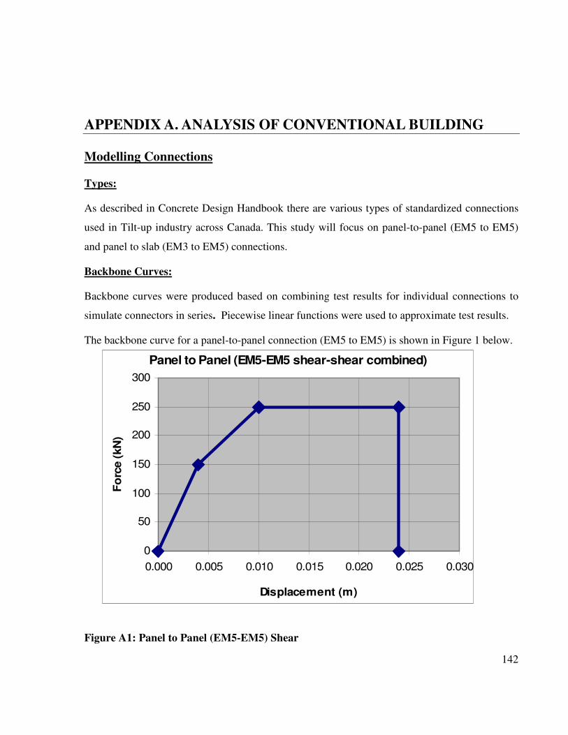
142
APPENDIX A. ANALYSIS OF CONVENTIONAL BUILDING
Modelling Connections
Types:
As described in Concrete Design Handbook there are various types of standardized connections
used in Tilt-up industry across Canada. This study will focus on panel-to-panel (EM5 to EM5)
and panel to slab (EM3 to EM5) connections.
Backbone Curves:
Backbone curves were produced based on combining test results for individual connections to
simulate connectors in series. Piecewise linear functions were used to approximate test results.
The backbone curve for a panel-to-panel connection (EM5 to EM5) is shown in Figure 1 below.
Figure A1: Panel to Panel (EM5-EM5) Shear
Panel to Panel (EM5-EM5 shear-shear combined)
0
50
100
150
200
250
300
0.000 0.005 0.010 0.015 0.020 0.025 0.030
Displacement (m)
Fo
rce (
kN
)
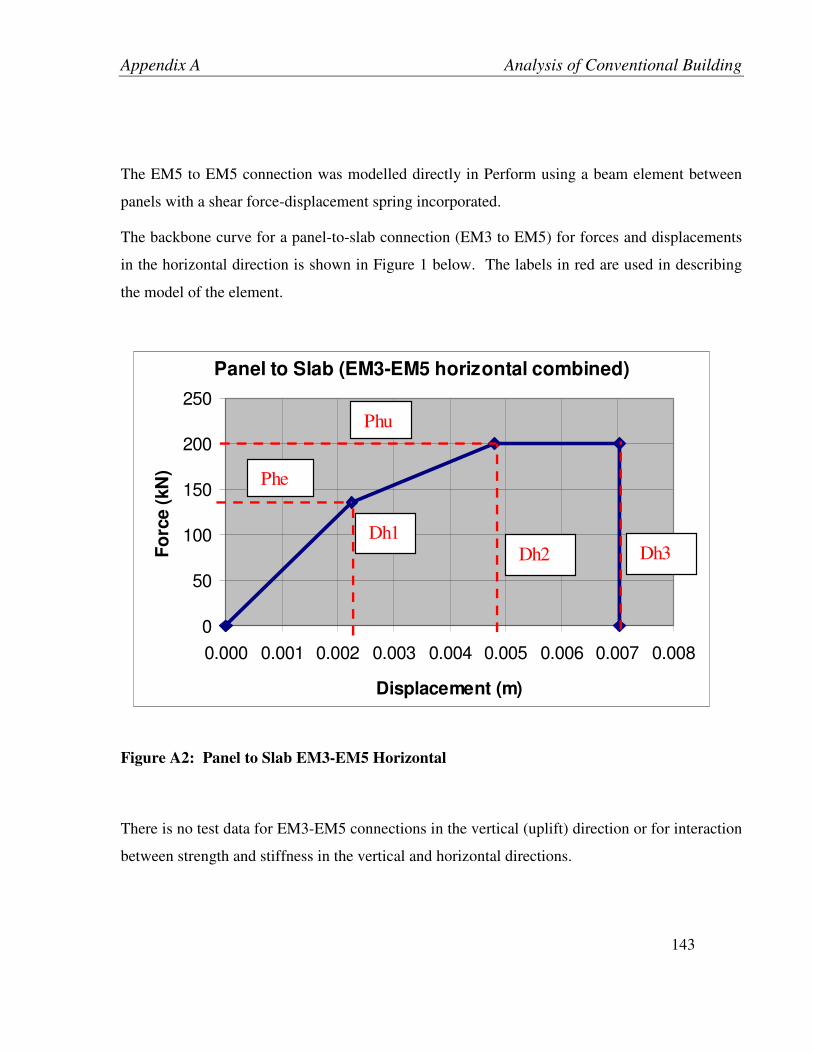
Appendix A Analysis of Conventional Building
143
The EM5 to EM5 connection was modelled directly in Perform using a beam element between
panels with a shear force-displacement spring incorporated.
The backbone curve for a panel-to-slab connection (EM3 to EM5) for forces and displacements
in the horizontal direction is shown in Figure 1 below. The labels in red are used in describing
the model of the element.
Figure A2: Panel to Slab EM3-EM5 Horizontal
There is no test data for EM3-EM5 connections in the vertical (uplift) direction or for interaction
between strength and stiffness in the vertical and horizontal directions.
Panel to Slab (EM3-EM5 horizontal combined)
0
50
100
150
200
250
0.000 0.001 0.002 0.003 0.004 0.005 0.006 0.007 0.008
Displacement (m)
Fo
rce (
kN
)
Dh2
Phu
Dh1
Phe
Dh3

Appendix A Analysis of Conventional Building
144
The strength in the vertical direction was approximated as follows:
• A failure cone was assumed as shown in Figure3 below, in which the bar bends approximately 50mm from the edge of the angle.
• The pullout strength of the resulting concrete wedge is approximately as follows: o Pullout Area Ac = 70mm*100mm – 50mm*20mm = 6000 mm2 o Concrete Strength, fc’ = 30MPa
Figure A3: Sketch of Assumed Concrete Pullout Failure in the EM5 Connector for Forces
in the “Vertical” Direction
Dh = Ac*0.3*(fc’)0.5 = 10 kN

Appendix A Analysis of Conventional Building
145
• The bending strength of the bars is approximately as follows: o Moment Resistance of Bars,
o Bar Yield Strength, Fy = 400Mpa
o Bar Diameter, d = 16mm
o Based on bending moment diagram below,
o Equate applied moment and moment resistance, therefore maximum applied
force,
Figure A4: Sketch of Assumed Mechanism in the EM5 Connector for Forces in the
“Vertical” Direction
Mr = Fy*Sx = Fy*π*d3/32 = 0.16 kNm
Mf = 0.0125*P kNm
P = (0.16 kNm) / (0.0125m) = 13 kN
P
0.5*P 0.5*P
50mm
Mf = 0.5*P*(0.05m)/2
0.0125*P kNm
BMD
15M bar
L38x38
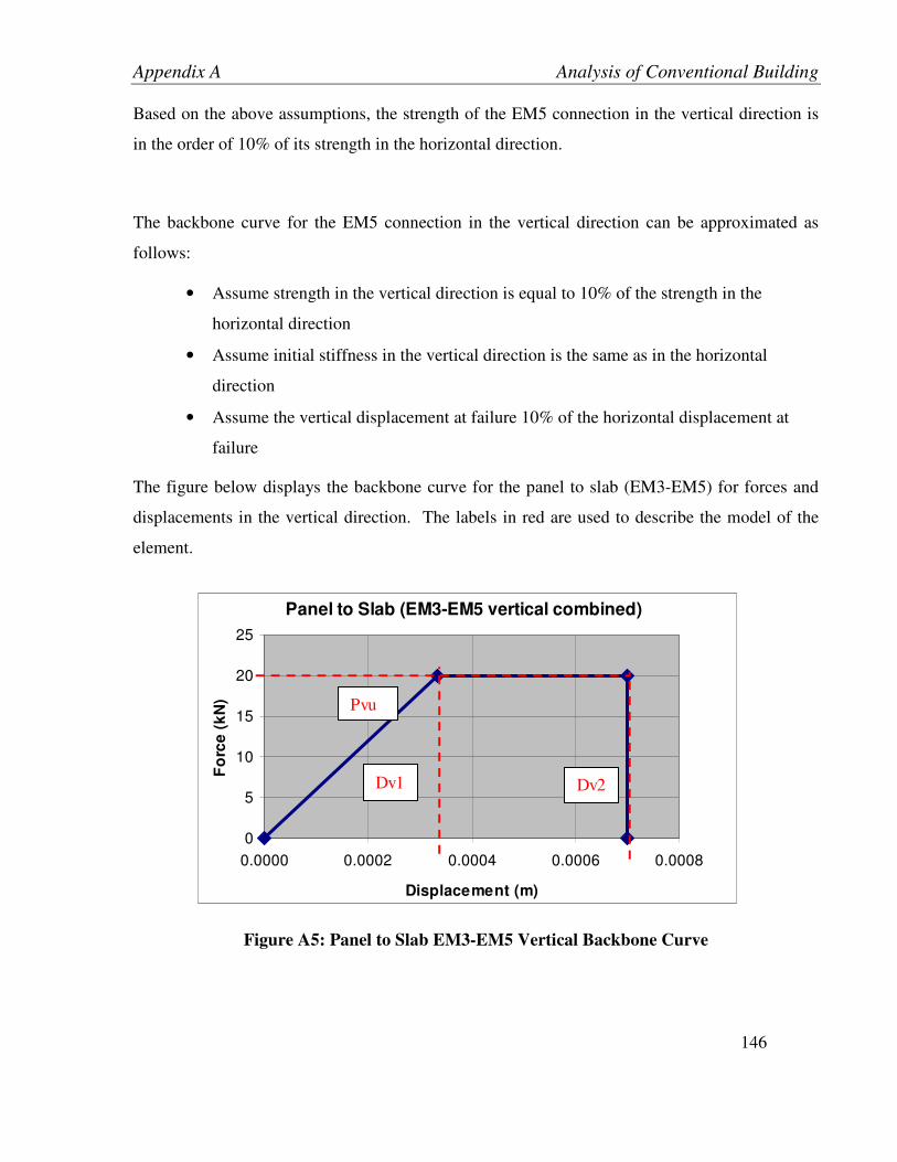
Appendix A Analysis of Conventional Building
146
Based on the above assumptions, the strength of the EM5 connection in the vertical direction is
in the order of 10% of its strength in the horizontal direction.
The backbone curve for the EM5 connection in the vertical direction can be approximated as
follows:
• Assume strength in the vertical direction is equal to 10% of the strength in the
horizontal direction
• Assume initial stiffness in the vertical direction is the same as in the horizontal
direction
• Assume the vertical displacement at failure 10% of the horizontal displacement at
failure
The figure below displays the backbone curve for the panel to slab (EM3-EM5) for forces and
displacements in the vertical direction. The labels in red are used to describe the model of the
element.
Figure A5: Panel to Slab EM3-EM5 Vertical Backbone Curve
Panel to Slab (EM3-EM5 vertical combined)
0
5
10
15
20
25
0.0000 0.0002 0.0004 0.0006 0.0008
Displacement (m)
Fo
rce
(k
N) Pvu
Dv1 Dv2
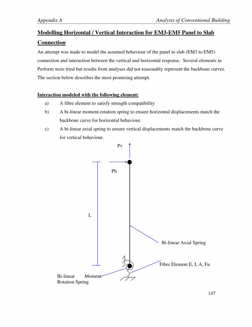
Appendix A Analysis of Conventional Building
147
Modelling Horizontal / Vertical Interaction for EM3-EM5 Panel to Slab
Connection
An attempt was made to model the assumed behaviour of the panel to slab (EM3 to EM5)
connection and interaction between the vertical and horizontal response. Several elements in
Perform were tried but results from analyses did not reasonably represent the backbone curves.
The section below describes the most promising attempt.
Interaction modeled with the following element:
a) A fibre element to satisfy strength compatibility
b) A bi-linear moment-rotation spring to ensure horizontal displacements match the
backbone curve for horizontal behaviour.
c) A bi-linear axial spring to ensure vertical displacements match the backbone curve
for vertical behaviour.
Fibre Element E, I, A, Fu
Pv
Ph
L
Bi-linear Axial Spring
Bi-linear Moment Rotation Spring

Appendix A Analysis of Conventional Building
148
Figure A6: Element used to model vertical/horizontal interaction for EM3-EM5
connections
Properties of Fibre Element:
• Bending properties used to model horizontal strength
• Axial properties used to model vertical strength
Figure A7: Cross-section of fibre element
PERFORM calculates moment of inertia as follows: I = A*y2 (a)
To satisfy strength compatibility between axial and moment:
For axial (vertical): A
PvFu u= (b)
For moment (horizontal): yA
LPh
yA
yLPh
I
yMFu u
*
)*5.0(*
*
**5.0**2
=== (c)
Equate equation (b) and (c): uPv
LPhy
*5.0*= (d)
Note that (0.5*L) used for the moment arm because the fibre element assumes constant curvature
over the element length and utilizes the curvature in the middle of the element to carry out
calculations.
y
A/2
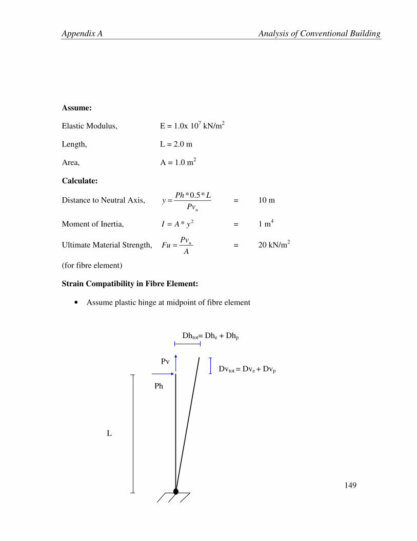
Appendix A Analysis of Conventional Building
149
Assume:
Elastic Modulus, E = 1.0x 10⁷ kN/m2
Length, L = 2.0 m
Area, A = 1.0 m2
Calculate:
Distance to Neutral Axis, uPv
LPhy
*5.0*= = 10 m
Moment of Inertia, 2* yAI = = 1 m4
Ultimate Material Strength, A
PvFu u= = 20 kN/m2
(for fibre element)
Strain Compatibility in Fibre Element:
• Assume plastic hinge at midpoint of fibre element
Dhtot= Dhe + Dhp
Dvtot = Dve + Dvp Pv
Ph
L

Appendix A Analysis of Conventional Building
150
Figure A8: Fibre element displacements
Displacements from Backbone Curves:
Horizontal Elastic, Dhe = Dh1 = 0.0048m
Plastic, Dhp = Dh3-Dh2 = 0.0022m
Vertical Elastic, Dve = Dv1 = 0.00033m
Plastic, Dvp = Dv2 – Dv1 = 0.00037m
Strain in Fibre Element due to Bending:
Plastic Rotation at Hinge, L
Dhp
p
*5.0=θ = 0.00223 radians
Figure A9: Strain in Fibre Element Due to Bending
Plastic Strain in fibre, L
ypp
*θε = = 0.011
Elastic Strain in fibre, E
Fue =ε = 2.0 x 10⁻⁶
θp
εp
y

Appendix A Analysis of Conventional Building
151
Strain at which strength loss occurs, epu εεε += = 0.011
Strain In Fibre Element Due to Axial Loads:
Plastic Strain in fibre, L
Dyp =ε = 0.000183
Elastic Strain in fibre, E
Fue =ε = 0.000002
Strain at which strength loss occurs, εu = εp + εe = 0.0001853
The plastic strains required to achieve the required horizontal and vertical plastic
displacements are not the same. Use the strain required to match the vertical backbone
displacements in the analysis, since it is more conservative (less ductile)
Properties of Bi-linear Axial Spring
• Used to model the non-linear characteristics of vertical backbone curve prior to ultimate
Initial Stiffness, 1Dv
PvKi e= = 20093 kN/m
Yielded Stiffness, 12 DvDv
PvPvKy
ey
−
−= = 0 kN/m
Ratio of Yielded to Initial Stiffness, Ki
Ky = 0

Appendix A Analysis of Conventional Building
152
Since axial spring acting in series with fibre element, must account for axial stiffness of
fibre element:
Figure A10: Axial spring to model stiffness of vertical backbone
Vertical displacement in fibre element at yield,AE
LPvDv e
fe *
*= = 4.0 x 10⁻⁶ m
Panel to Slab (EM3-EM5 vertical combined)
0
5
10
15
20
25
0.0000 0.0002 0.0004 0.0006 0.0008Displacement (m)
Fo
rce
(k
N)
Dvf u
Fibre Element
linear axial
spring
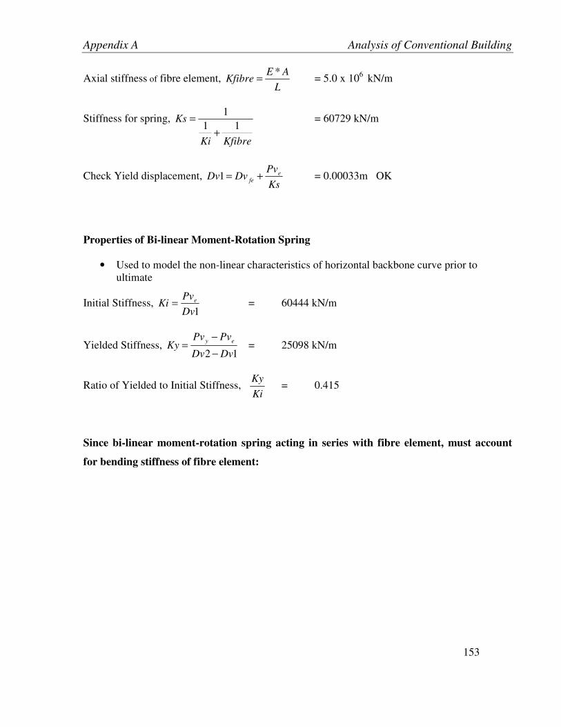
Appendix A Analysis of Conventional Building
153
Axial stiffness of fibre element, L
AEKfibre
*= = 5.0 x 10⁶ kN/m
Stiffness for spring,
KfibreKi
Ks11
1
+
= = 60729 kN/m
Check Yield displacement, Ks
PvDvDv e
fe +=1 = 0.00033m OK
Properties of Bi-linear Moment-Rotation Spring
• Used to model the non-linear characteristics of horizontal backbone curve prior to ultimate
Initial Stiffness, 1Dv
PvKi e= = 60444 kN/m
Yielded Stiffness, 12 DvDv
PvPvKy
ey
−
−= = 25098 kN/m
Ratio of Yielded to Initial Stiffness, Ki
Ky = 0.415
Since bi-linear moment-rotation spring acting in series with fibre element, must account
for bending stiffness of fibre element:
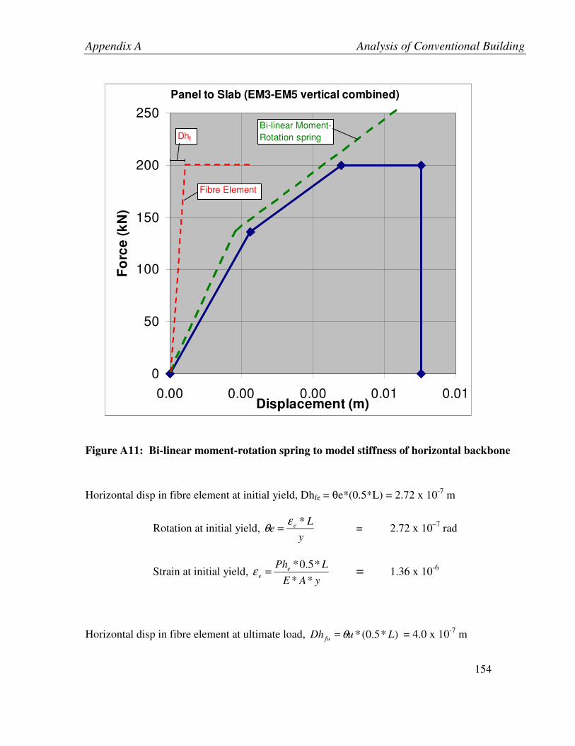
Appendix A Analysis of Conventional Building
154
Figure A11: Bi-linear moment-rotation spring to model stiffness of horizontal backbone
Horizontal disp in fibre element at initial yield, Dhfe = θe*(0.5*L) = 2.72 x 10⁻⁷ m
Rotation at initial yield, y
Le e *ε
θ = = 2.72 x 10⁻⁷ rad
Strain at initial yield, yAE
LPhee **
*5.0*=ε = 1.36 x 10⁻⁶
Horizontal disp in fibre element at ultimate load, )*5.0(* LuDh fu θ= = 4.0 x 10⁻⁷ m
Panel to Slab (EM3-EM5 vertical combined)
0
50
100
150
200
250
0.00 0.00 0.00 0.01 0.01Displacement (m)
Fo
rce
(k
N)
Dhf
Fibre Element
Bi-linear Moment-
Rotation spring

Appendix A Analysis of Conventional Building
155
Rotation at initial yield, y
Lu u *ε
θ = = 4.0x 10⁻⁷ rad
Strain at initial yield, yAE
LPhuu **
*5.0*=ε = 2.0 x 10⁻⁶
Horizontal stiffness of fibre element, fu
u
Dh
PhKfibre = = 5.00 x 10⁸ kN/m
Initial Stiffness for spring,
KfibreKi
Ksi11
1
+
= = 60452 kN/m
Yielded Stiffness for spring,
KfibreKy
Ksy11
1
+
= = 25099 kN/m
Relationship between rotational and horizontal stiffness:
Horizontal Stiffness, 2*
*L
M
L
L
M
Dh
PhKs
fu
u
θθ
===
Solve for Moment, M = Ks*θ*L2
Figure A12: Relationship between horizontal and rotational stiffness
Initial rotational stiffness, 2* LKsiM
Ksi ==θ
θ = 241807 kNm/rad
Yielded rotational stiffness, 2* LKsiM
Ksy ==θ
θ = 100397 kNm/rad
Check Yield displacement, Ksi
PhDhDh e
fe +=1 = 0.00225 m
Dh
Ph
L
θ
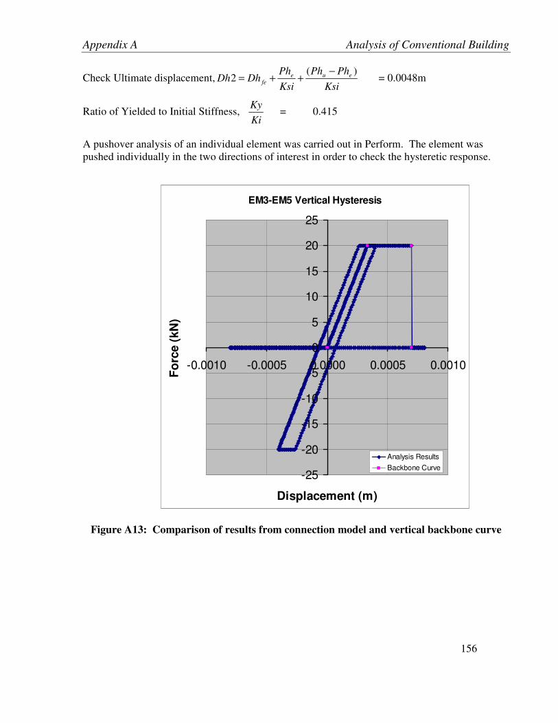
Appendix A Analysis of Conventional Building
156
Check Ultimate displacement,Ksi
PhPh
Ksi
PhDhDh eue
fe
)(2
−++= = 0.0048m
Ratio of Yielded to Initial Stiffness, Ki
Ky = 0.415
A pushover analysis of an individual element was carried out in Perform. The element was pushed individually in the two directions of interest in order to check the hysteretic response.
Figure A13: Comparison of results from connection model and vertical backbone curve
EM3-EM5 Vertical Hysteresis
-25
-20
-15
-10
-5
0
5
10
15
20
25
-0.0010 -0.0005 0.0000 0.0005 0.0010
Displacement (m)
Fo
rce (
kN
)
Analysis Results
Backbone Curve

Appendix A Analysis of Conventional Building
157
Figure A14: Comparison of results from connection model and horizontal backbone curve
As can be seen from above figures, there is good agreement between the model and the
backbone curves. The envelope of hysteretic response matches closely with the backbone
curves.
The ductility of the vertical backbone is captured, but the full ductility of the horizontal
backbone is not, due to the incompatibility in strains described in the section above.
EM3-EM5 Horizontal Hysteresis
-200
-150
-100
-50
0
50
100
150
200
250
-0.010 -0.005 0.000 0.005 0.010
Displacement (m)
Fo
rce (
kN
)
Analysis Results
Backbone Curve

Appendix A Analysis of Conventional Building
158
Testing of Elements Used to Model EM3-EM5 Panel to Slab Connections with
a 2-Panel Model
Model Description
In the two-panel model, five EM5-EM5 connectors were used between panels to ensure that
there would be little deformation between panels. Three EM3-EM5 connectors were used per
panel, incorporating the assumptions described in the section above. The stiffness of the panels
was increased so that the panels were essentially rigid. The figure below shows a sketch of the
two-panel model. The panel to slab connectors are numbered c1 to c6 for tracking the connector
response.
Figure A15: Sketch of two-panel model
Loading Protocol:
The model was subjected to a point load at a height of 8.5m and pushed to a roof drift of 0.002,
then pushed in the opposite direction to a roof drift of –0.002, and then back to zero. The cycle
was then repeated. The figure below is a screen capture from the PERFORM model at a roof
drift of 0.002.
c1 c3 c4 c5 c6 c2
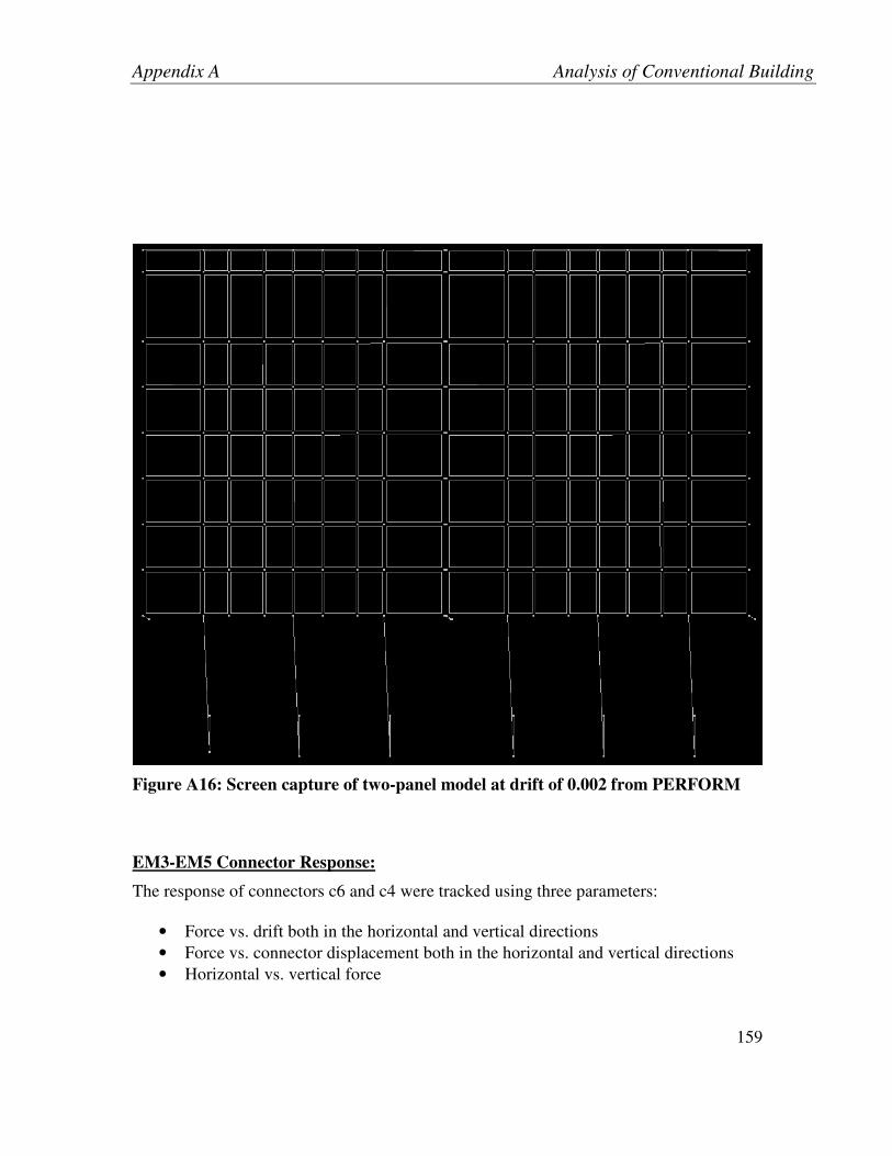
Appendix A Analysis of Conventional Building
159
Figure A16: Screen capture of two-panel model at drift of 0.002 from PERFORM
EM3-EM5 Connector Response:
The response of connectors c6 and c4 were tracked using three parameters:
• Force vs. drift both in the horizontal and vertical directions • Force vs. connector displacement both in the horizontal and vertical directions • Horizontal vs. vertical force
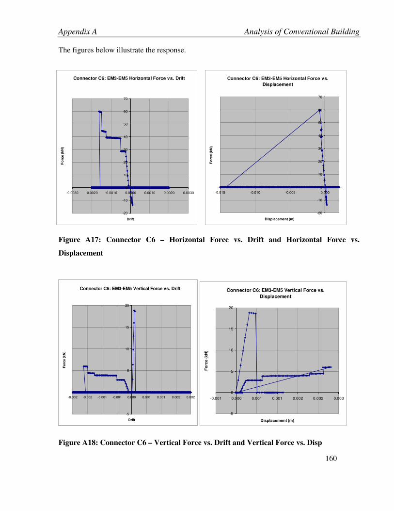
Appendix A Analysis of Conventional Building
160
The figures below illustrate the response.
Figure A17: Connector C6 – Horizontal Force vs. Drift and Horizontal Force vs.
Displacement
Figure A18: Connector C6 – Vertical Force vs. Drift and Vertical Force vs. Disp
Connector C6: EM3-EM5 Horizontal Force vs.
Displacement
-20
-10
0
10
20
30
40
50
60
70
-0.015 -0.010 -0.005 0.000
Displacement (m)
Fo
rce
(k
N)
Connector C6: EM3-EM5 Horizontal Force vs. Drift
-20
-10
0
10
20
30
40
50
60
70
-0.0030 -0.0020 -0.0010 0.0000 0.0010 0.0020 0.0030
Drift
Fo
rce
(k
N)
Connector C6: EM3-EM5 Vertical Force vs. Drift
-5
0
5
10
15
20
-0.002 -0.002 -0.001 -0.001 0.000 0.001 0.001 0.002 0.002
Drift
Fo
rce
(k
N)
Connector C6: EM3-EM5 Vertical Force vs.
Displacement
-5
0
5
10
15
20
-0.001 0.000 0.001 0.001 0.002 0.002 0.003
Displacement (m)
Fo
rce
(k
N)

Appendix A Analysis of Conventional Building
161
Figure A19: Connector C6 – Horizontal Force vs. Vertical Force
Discussion:
In Figures 15 and 16, it can be observed that when the model is pushed in the first direction (to a
drift of 0.002), the EM3 – EM5 element behaves reasonably well. The response in the vertical
and horizontal directions corresponds with the backbone curves until a strength limit is reached
due to the interaction between the two. This occurs at a horizontal shear force in the connector of
approximately 13 kN (ultimate strength = 200kN) and a vertical force of approximately 19 kN
(ultimate strength = 20kN). This indicates the element obeys the interaction constraints, since
13/200 + 19/20 = 1.0. Once the element reaches this strength limit, both the horizontal and
vertical forces drop down to zero.
Connector C6: EM3-EM5 Horizontal Force vs.
Vertical Force
-20
-10
0
10
20
30
40
50
60
70
-5 0 5 10 15 20
Vertical Force (kN)
Ho
rizo
nta
l F
orc
e (
kN
)
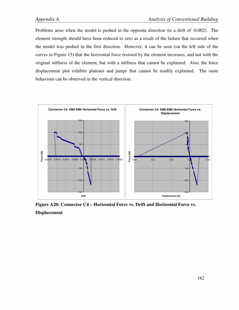
Appendix A Analysis of Conventional Building
162
Problems arise when the model is pushed in the opposite direction (to a drift of -0.002). The
element strength should have been reduced to zero as a result of the failure that occurred when
the model was pushed in the first direction. However, it can be seen (on the left side of the
curves in Figure 15) that the horizontal force resisted by the element increases, and not with the
original stiffness of the element, but with a stiffness that cannot be explained. Also, the force
displacement plot exhibits plateaus and jumps that cannot be readily explained. The same
behaviour can be observed in the vertical direction.
Figure A20: Connector C4 – Horizontal Force vs. Drift and Horizontal Force vs.
Displacement
Connector C4: EM3-EM5 Horizontal Force vs. Drift
-150
-100
-50
0
50
100
150
-0.0020 -0.0015 -0.0010 -0.0005 0.0000 0.0005 0.0010 0.0015 0.0020
Drift
Fo
rce
(k
N)
Connector C4: EM3-EM5 Horizontal Force vs.
Displacement
-150
-100
-50
0
50
100
150
-0.02 -0.01 -0.01 0.00 0.01
Displacement (m)
Fo
rce
(k
N)

Appendix A Analysis of Conventional Building
163
Figure A21: Connector C4 – Vertical Force vs. Drift and Vertical Force vs. Displacement
Figure A22: Connector C4 – Horizontal Force vs. Vertical Force
Connector C4: EM3-EM5 Horizontal Force vs.
Vertical Force
-200
-150
-100
-50
0
50
100
150
200
-5 0 5 10 15 20
Vertical Force (kN)
Ho
rizo
nta
l F
orc
e (kN
)
Interaction Line
Connector C4: EM3-EM5 Vertical Force vs. Drift
-2
0
2
4
6
8
10
12
14
-0.003 -0.002 -0.001 0.000 0.001 0.002 0.003
Drift
Fo
rce
(k
N)
Connector C4: EM3-EM5 Vertical Force vs.
Displacement
-2
0
2
4
6
8
10
12
14
-0.002 0.000 0.002 0.004 0.006 0.008 0.010
Displacement (m)
Fo
rce
(k
N)
Appendix A Analysis of Conventional Building
164
Discussion:
Connector c4 displays the same type of behaviour as connector c6, except that the horizontal
force reaches a greater value and the vertical force in the connector reaches a lesser value at the
interaction point. This is reasonable considering their respective positions. However, connector
c4 displays the same unexplained behaviour when the model is pushed to a drift of –0.002.
The interaction between the horizontal force and vertical force can be clearly observed in Figure
20, in which the recorded plot closely follows the predicted interaction line for the element.
Due to the problems observed with the element response, this element was not used in the
analysis

165
APPENDIX B. DESIGN NOTES AND MODEL PROPERTIES
FOR ARCHETYPICAL SYSTEM 1: SOLID WALL PANELS
Design of Solid Panels for Vertical and Out-of-Plane Loading
Assumptions:
1. Building located in Vancouver, B.C., site class D
References:
1. CAN/CSA A23.3
2. "Concrete Design Handbook - Third Edition" by the Cement Association of Canada
Material Properties:
Concrete material factor Φc = 0.65
Reinf Steel material factor Φs = 0.85
Member resistance factor Φm = 0.75
Reinf Steel yield strength fy = 400 MPa
Concrete compressive strength
fc' = 30 MPa
Modulus of Rupture fr = 0.6*(fc')^0.5
= 3.3 MPa
Concrete tangent modulus Ec = 4500(fc')^0.5
= 24648 MPa
a1 = 0.85-0.0015*fc'
= 0.805
B1 = 0.97-0.0025*fc'
= 0.895
Reinf Steel Elastic modulus Es = 200000 MPa
Concrete unit weight wc = 24 kN/m
3
Wall Panel Properties:
Height h = 9144 mm
thickness t = 184 mm
initial deflection ∆o = 25 mm
check span to depth ratio h/t = 50
OK for 1 layer of reinforcing
concrete cover c = 32 mm
Loading:
Roof Joist Span L = 15.24 m

Appendix B Design Notes and Model Properties for Archetypical System 1
166
wall self weight qwall = wc*t
= 4.416 kN/m
2
Roof Self Wt. qroof = 1.0 kN/m
2
Snow Load (NBCC 2005 Cl qsnow = Is*(Ss*(Cb*Cb*Cs*Ca)+Sr)
For tilt-up building in Vancouver:
Is = Ss = Cw = Cs = Ca = 1.0, Cb = 0.8
Ss = 1.8 kN/m
2
Sr = 0.2
Design Snow Load qsnow = 1.6 kN/m
2
Wind Load (NBCC 2005 Cl 4.1.7)
qwind = Iw*q*Ce*(Cp*Cg + Cpi*Cgi)
1 in 50 velocity pressure q = 0.48 kN/m2
Importance Factor Iw = 1
Exposure Factor Ce = 1
Exterior Gust Coeff Cp*Cg = 1.3 or -1.5 (positive denotes towards surface, neg denotes away)
Interior Pressure Coeff Cpi = 0.3 of -0.45
Interior Gust Coeff Cgi = 2
Inward pressure qwind
inward = 1.0*q*1.0*(1.3 + 0.45*2.0)
Outward pressure qwind
outward = 1.0*q*1.0*(-1.5 - 0.3*2.0)
Inward pressure governs
Design Wind Load qwind = 1.06 kN/m2
Eccentricity ecc = t/2
= 92 mm
Seismic for Out-of-Plane forces (NBCC 2005 Cl 4.1.8.17)
Vp = 0.3*Fa*Sa(0.2)*Ie*Sp*Wp
Soil Modification Factor Fa = 1.1
(For Site Class D)
Spectral Acceleration at T=0.2s
Sa(0.2) = 0.94 g
Importance Factor Ie = 1.0
Sp = Cp*Ar*Ax / Rp
where 0.7<Sp<4.0
Component Risk Factor Cp = 1.0
Dynamic Amplification Factor
Ar = 1.0
(Typically used for tilt-up but maybe unconservative)
Height Factor Ax = 1+ 2*hx/hn
hx = Height of component above base
= Centre of mass of panel
hn = total height
Ax = 2
Response Factor Rp = 2.5
(for reinforced tilt-up wall panels)
Sp = 0.8

Appendix B Design Notes and Model Properties for Archetypical System 1
167
Seismic for Out-of-Plane forces
Vp = 0.248 *Wp
Compare Seismic to Wind (for 1m unit strip) Factored Seismic out-of-plane
qseismic = Vp*1.0m*qwall
= 1.10 kN/m
Factored Wind 1.5*qwind = 1.58 kN/m
Wind Governs for Out-of-Plane Loading on Panels
Strength Calculations:
Load Case (4): 1.25D + 1.4W + 0.5S
Factored Load from tributary roof area
Ptf = (1.25*qroof+0.5*qsnow)*L/2
= 15.8 kN/m
Factored weight of panel tributary to and above design section
Pwf = 1.25*qwall*h/2
= 25.2 kN/m
Axial Load at mid-height Pf = Ptf + Pwf
= 41.0 kN/m
Factored UDL lateral load wf = 1.4*qwind
= 1.5 kN/m
2
Check axial load limit Pf / Ag < 0.09*Φc*fc'
0.22 < 1.755 MPa OK
Assume reinforcing on each face (EF):
Reinforcing Steel Provided 15M @ 400 EF
Area of reinf steel (per face) As = 500 mm
2/m EF
Reinforcing Steel Ratio p = 2*As/(1000*t)
(both faces)
= 0.0054
Effective depth d = t-c-db/2 mm
= 144 mm
Width of design strip b = 1000 mm
Effective steel area Ase = (Φs*As*fy + Pf*1000) / (Φs*fy)
= 621 mm
2/m
Compressive stress block ae = Φs*Ase*fy / (a1*Φc*fc'*1000)
= 13.4 mm
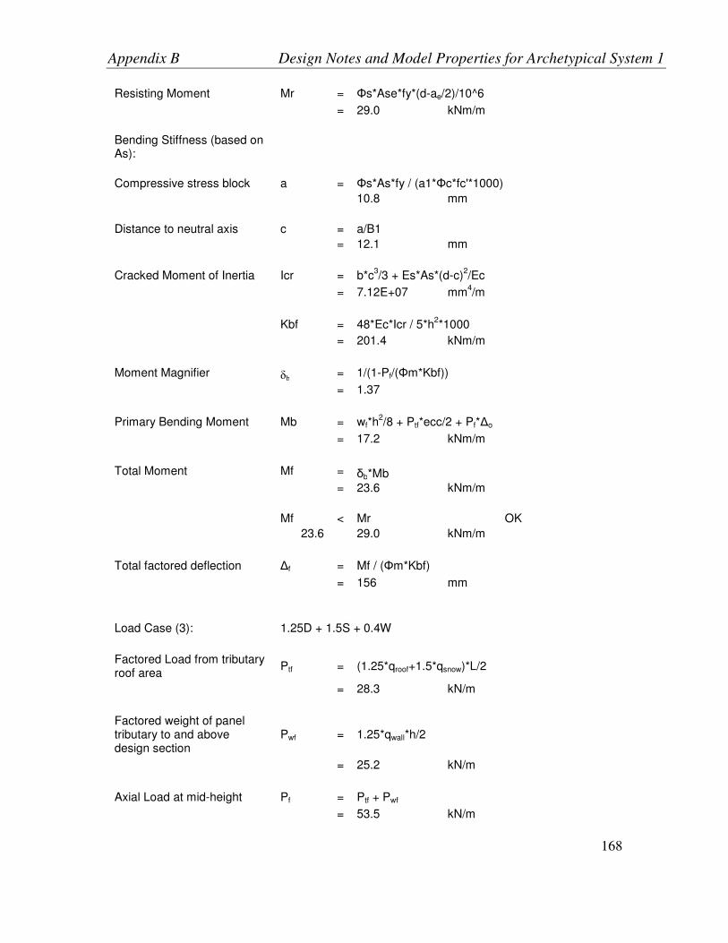
Appendix B Design Notes and Model Properties for Archetypical System 1
168
Resisting Moment Mr = Φs*Ase*fy*(d-ae/2)/10^6
= 29.0 kNm/m
Bending Stiffness (based on As):
Compressive stress block a = Φs*As*fy / (a1*Φc*fc'*1000)
10.8 mm
Distance to neutral axis c = a/B1
= 12.1 mm
Cracked Moment of Inertia Icr = b*c
3/3 + Es*As*(d-c)
2/Ec
= 7.12E+07 mm
4/m
Kbf = 48*Ec*Icr / 5*h
2*1000
= 201.4 kNm/m
Moment Magnifier δb = 1/(1-Pf/(Φm*Kbf))
= 1.37
Primary Bending Moment Mb = wf*h
2/8 + Ptf*ecc/2 + Pf*∆o
= 17.2 kNm/m
Total Moment Mf = δb*Mb
= 23.6 kNm/m
Mf < Mr
OK
23.6
29.0 kNm/m
Total factored deflection ∆f = Mf / (Φm*Kbf)
= 156 mm
Load Case (3): 1.25D + 1.5S + 0.4W
Factored Load from tributary roof area
Ptf = (1.25*qroof+1.5*qsnow)*L/2
= 28.3 kN/m
Factored weight of panel tributary to and above design section
Pwf = 1.25*qwall*h/2
= 25.2 kN/m
Axial Load at mid-height Pf = Ptf + Pwf
= 53.5 kN/m

Appendix B Design Notes and Model Properties for Archetypical System 1
169
Factored UDL lateral load wf = 0.4*qwind
= 0.42 kN/m
2
Assume reinforcing on each face (EF):
Reinforcing Steel Provided 15M @ 400 EF
Area of reinf steel As = 500 mm
2/m EF
Effective steel area Ase = (Φs*As*fy + Pf*1000) / (Φs*fy)
= 657 mm
2/m
Compressive stress block ae = Φs*Ase*fy / (a1*Φc*fc'*1000)
= 14.2 mm
Resisting Moment Mr = Φs*Ase*fy*(d-ae/2)/10^6
= 30.6 kNm/m
Bending Stiffness (based on As):
Compressive stress block a = Φs*As*fy / (a1*Φc*fc'*1000)
10.8 mm
Distance to neutral axis c = a/B1
= 12.1 mm
Cracked Moment of Inertia Icr = b*c
3/3 + Es*As*(d-c)
2/Ec
= 7.12E+07 mm
4/m
Kbf = 48*Ec*Icr / 5*h
2*1000
= 201.4 kNm/m
Moment Magnifier δb = 1/(1-Pf/(Φm*Kbf))
= 1.55
Primary Bending Moment Mb = wf*h
2/8 + Ptf*ecc/2 + Pf*∆o
= 7.05 kNm/m
Total Moment Mf = δb*Mb
= 10.9 kNm/m
Mf < Mr
OK
10.9
30.6 kNm/m
Deflections at Service Loads
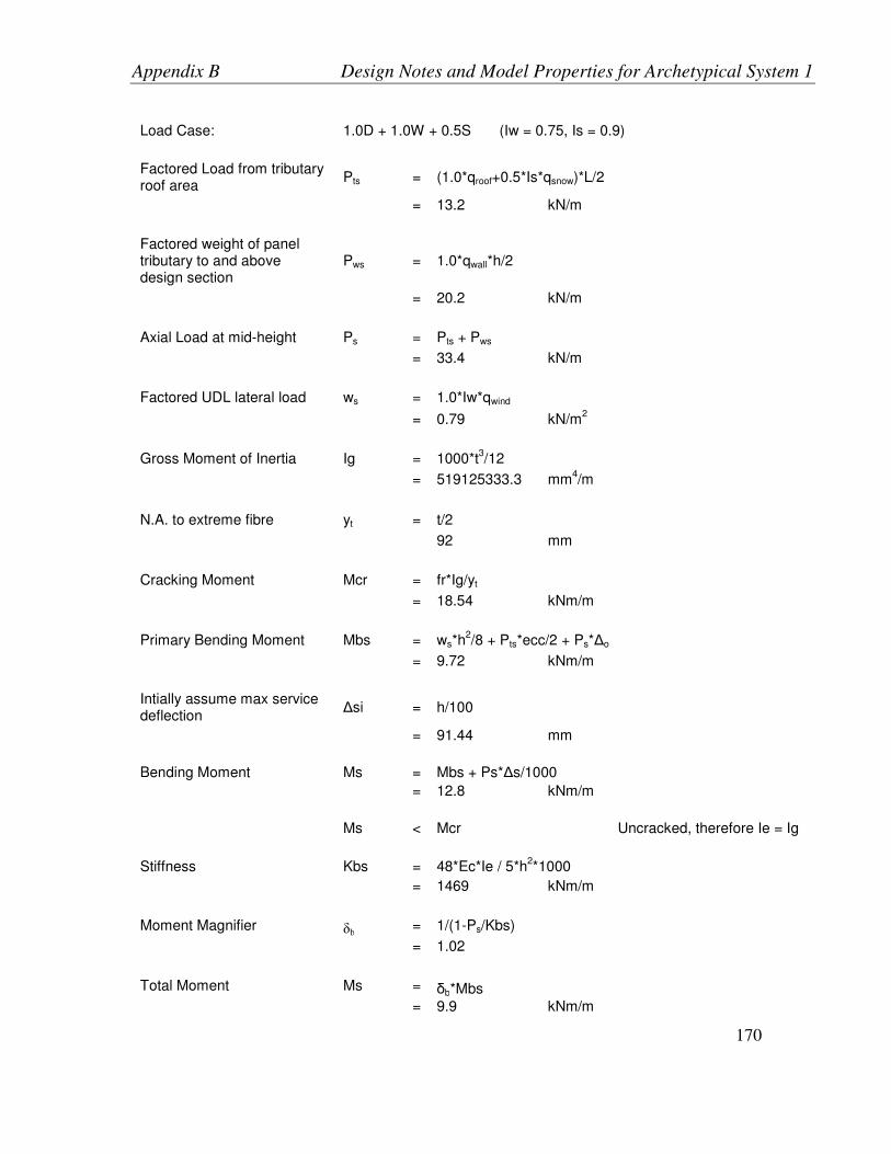
Appendix B Design Notes and Model Properties for Archetypical System 1
170
Load Case: 1.0D + 1.0W + 0.5S (Iw = 0.75, Is = 0.9)
Factored Load from tributary roof area
Pts = (1.0*qroof+0.5*Is*qsnow)*L/2
= 13.2 kN/m
Factored weight of panel tributary to and above design section
Pws = 1.0*qwall*h/2
= 20.2 kN/m
Axial Load at mid-height Ps = Pts + Pws
= 33.4 kN/m
Factored UDL lateral load ws = 1.0*Iw*qwind
= 0.79 kN/m
2
Gross Moment of Inertia Ig = 1000*t
3/12
= 519125333.3 mm
4/m
N.A. to extreme fibre yt = t/2
92 mm
Cracking Moment Mcr = fr*Ig/yt
= 18.54 kNm/m
Primary Bending Moment Mbs = ws*h
2/8 + Pts*ecc/2 + Ps*∆o
= 9.72 kNm/m
Intially assume max service deflection
∆si = h/100
= 91.44 mm
Bending Moment Ms = Mbs + Ps*∆s/1000
= 12.8 kNm/m
Ms < Mcr
Uncracked, therefore Ie = Ig
Stiffness Kbs = 48*Ec*Ie / 5*h
2*1000
= 1469 kNm/m
Moment Magnifier δb = 1/(1-Ps/Kbs)
= 1.02
Total Moment Ms = δb*Mbs
= 9.9 kNm/m

Appendix B Design Notes and Model Properties for Archetypical System 1
171
Ms < Mr
OK
9.9
18.5 kNm/m
max service deflection ∆s = Ms/Kbs*1000
= 6.8 mm
∆s < ∆si
OK
Panel Design Summary
Vertical Reinforcing 15M @ 400 EF
Steel Area As = 1000 mm
2/m
Reinforcing Steel Ratio p = As/(1000*t)
= 0.0054
Horizontal Reinforcing 15M @ 400 AF (alternating faces)
Steel Area As = 500 mm
2/m
Reinforcing Steel Ratio p = As/(1000*t)
= 0.0027
Design of Solid Panels for In-Plane
Loading Along Long Axis of Building
Assuming building located in Langely, B.C., site class C
Material Properties:
Concrete material factor
Φc = 0.65
Reinf Steel material factor Φs = 0.85
Member resistance factor Φm = 0.75
Reinf Steel yield strength fy = 400 MPa
Concrete compressive strength fc' = 30 MPa
Modulus of Rupture fr = 0.6*(fc')^0.5
= 3.3 MPa
Concrete tangent modulus Ec = 4500(fc')^0.5
= 24648 MPa
a1 = 0.85-0.0015*fc'
= 0.805
B1 = 0.97-0.0025*fc'
= 0.895
Reinf Steel Elastic modulus Es = 200000 MPa
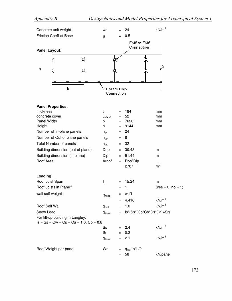
Appendix B Design Notes and Model Properties for Archetypical System 1
172
Concrete unit weight wc = 24 kN/m3
Friction Coeff at Base µ = 0.5
Panel Layout:
Panel Properties:
thickness t = 184 mm
concrete cover cover = 52 mm
Panel Width b = 7620 mm
Height h = 9144 mm
Number of In-plane panels nip = 24
Number of Out of plane panels nop = 8
Total Number of panels ntot = 32
Building dimension (out of plane) Dop = 30.48 m
Building dimension (in plane) Dip = 91.44 m
Roof Area Aroof = Dop*Dip
2787 m
2
Loading:
Roof Joist Span L = 15.24 m
Roof Joists in Plane? = 1 (yes = 0, no = 1)
wall self weight qwall = wc*t
= 4.416 kN/m
2
Roof Self Wt. qroof = 1.0 kN/m
2
Snow Load qsnow = Is*(Ss*(Cb*Cb*Cs*Ca)+Sr)
For tilt-up building in Langley:
Is = Ss = Cw = Cs = Ca = 1.0, Cb = 0.8
Ss = 2.4 kN/m
2
Sr = 0.2
qsnow = 2.1 kN/m
2
Roof Weight per panel Wr = qroof*b*L/2
= 58 kN/panel

Appendix B Design Notes and Model Properties for Archetypical System 1
173
Panel Weight Wp = qwall*(b*h)
= 308 kN/panel
Total Building Weight W = qroof*Aroof + ntot*Wp
= 12633 kN
Base Shear Calculation for Rd, Ro = 1.0 (NBCC 2005)
Building Period T = 0.05*h
3/4
= 0.26 s
T<2.0 seconds, and R=1.5, Therefire 2/3*S(0.2) applies
Spectral Acceleration S(0.2) = 1.1 g
Soil Modification Factor Fa = 1
Importance Factor I = 1.0
Higher Mode Factor Mv = 1
Seismic Acceleration E = 0.66*I*S*Fa*Mv / (Rd*Ro)
= 0.73 g
Force from Roof Diaphram Vroof = ((qroof+0.25*qsnow)*Aroof + Wp*nop*0.5)*E*0.5
= 1995 kN per one wall line
Panel Shear Vpanel = E*nip*Wp*0.5
2681 kN per one wall line
Total Base Shear Vf = Vroof +Vpanel
= 4675 kN per one wall line
Check Maximum Concrete Shear (Rd, Ro = 1)
Max concrete shear Vrmax = Φc*fc'*t*dv
dv = 0.8*Dip
= 73 m
Vrmax = 262469 kN
Vrmax > Vf OK
Panel Shear Resistance Vc = Φc*B1*0.18*(fc')
0.5*t*dv
= 7720 kN
Steel: 15M @ 400 AF
Steel area Av = 200 mm
2
spacing s = 400 mm
Vs = Φs*Av*fy*dv*cotθ/s
= 0.486*Av*dv/s (for θ=35 deg, Φs=0.85,

Appendix B Design Notes and Model Properties for Archetypical System 1
174
fy=400MPa)
= 17776 kN
Total Shear Strength Vr = Vc+Vs
= 25496 kN
Vr > Vf OK
Panel Sliding (Base Connections)
Assume welded connections with studded embedments (EM3 in walls to EM5 in slab)
Ductility factor Rd = 1 For EM3
Overstrength Ro = 1.3
Required Base Shear for Connector design
Vfreqd = Vf/(Rd*Ro) - friction
Vf/(Rd*Ro) - µ*Wp*nip/2
1750 kN per one wall line
Shear resistance VrEM3 = 110 kN / connection in panel (GOVERNS)
VrEM5 = 125 kN / connection in floor slab
No. of connections required per panel:
N = Vfreqd/(VrEM3*nip/2)
= 1.3
PROVIDE 2 BASE CONNECTIONS PER PANEL
Panel Overturning (Wall to Wall Connections)
Assume welded connections with rebar embedments (EM5 to EM5 in walls)
Ductility factor Rd = 1.5
Overstrength Ro = 1.3
Overturning Moment Mof = (Vroof*h + Vpanel*h/2) / (Rd*Ro)
= 15639 kNm
Resisting Moments
Panel and Roof Weight Mrweight = (nip/2)*(Wp+Wr)*b/2
= 16723 kNm
End connections Vr = 100 kN
Mrend = Vr*b
= 762 kNm
Total Resisting Moment Mr = Mrweight+Mrend
= 17485 kNm
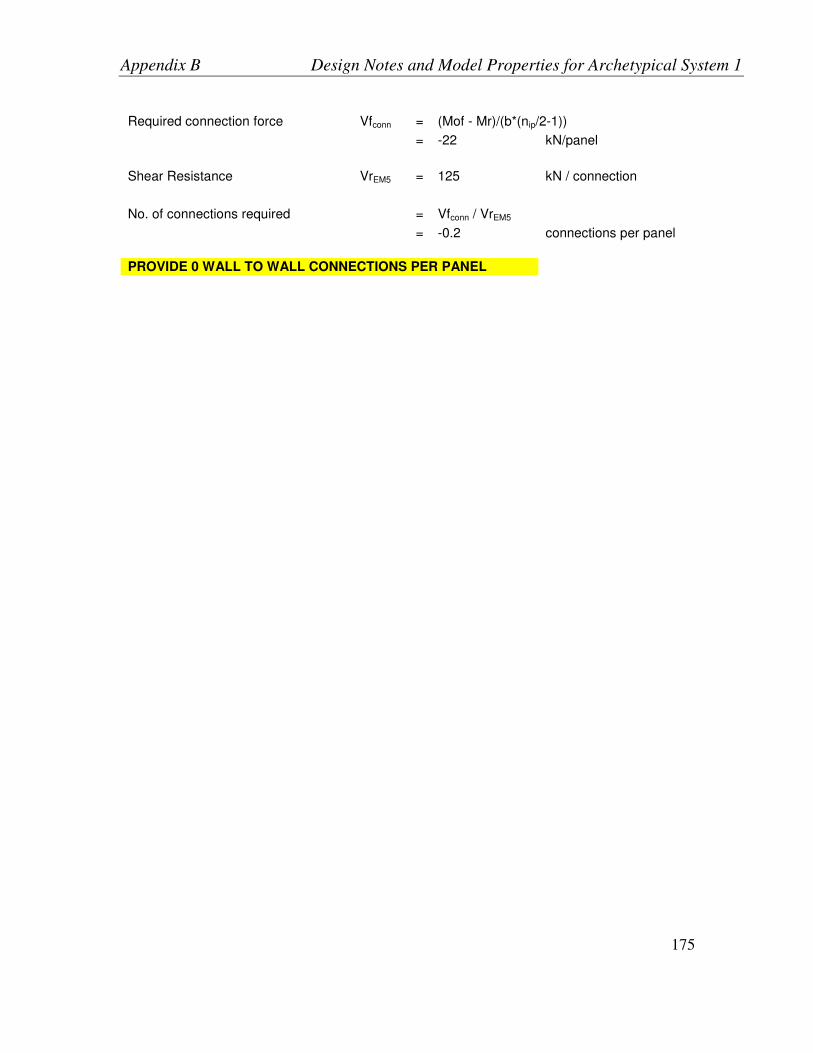
Appendix B Design Notes and Model Properties for Archetypical System 1
175
Required connection force Vfconn = (Mof - Mr)/(b*(nip/2-1))
= -22 kN/panel
Shear Resistance VrEM5 = 125 kN / connection
No. of connections required
= Vfconn / VrEM5
= -0.2 connections per panel
PROVIDE 0 WALL TO WALL CONNECTIONS PER PANEL
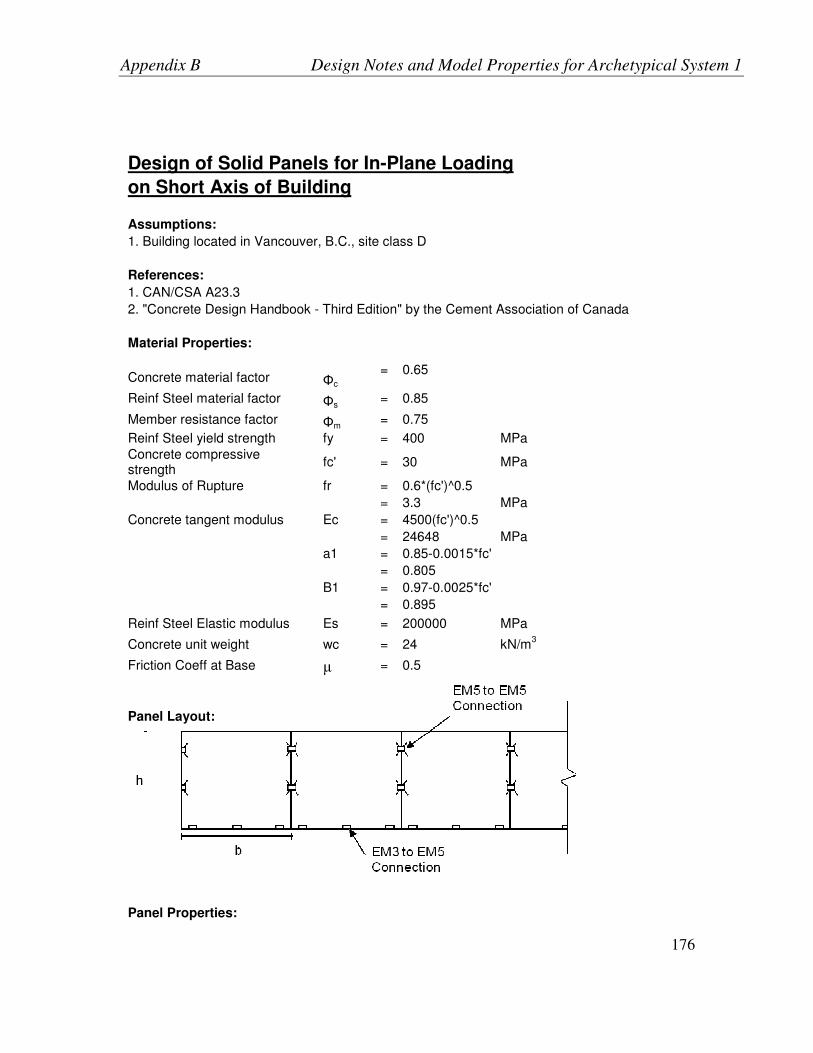
Appendix B Design Notes and Model Properties for Archetypical System 1
176
Design of Solid Panels for In-Plane Loading
on Short Axis of Building
Assumptions:
1. Building located in Vancouver, B.C., site class D
References:
1. CAN/CSA A23.3
2. "Concrete Design Handbook - Third Edition" by the Cement Association of Canada
Material Properties:
Concrete material factor
Φc = 0.65
Reinf Steel material factor Φs = 0.85
Member resistance factor Φm = 0.75
Reinf Steel yield strength fy = 400 MPa
Concrete compressive strength
fc' = 30 MPa
Modulus of Rupture fr = 0.6*(fc')^0.5
= 3.3 MPa
Concrete tangent modulus Ec = 4500(fc')^0.5
= 24648 MPa
a1 = 0.85-0.0015*fc'
= 0.805
B1 = 0.97-0.0025*fc'
= 0.895
Reinf Steel Elastic modulus Es = 200000 MPa
Concrete unit weight wc = 24 kN/m
3
Friction Coeff at Base µ = 0.5
Panel Layout:
Panel Properties:

Appendix B Design Notes and Model Properties for Archetypical System 1
177
thickness t = 184 mm
concrete cover cover = 52 mm
Panel Width b = 7620 mm
Height h = 9144 mm
Number of In-plane panels nip = 8
Number of Out of plane panels
nop = 24
Total Number of panels ntot = 32
Building Length (out of plane) L = 60.96 m
Building Width (in plane) w = 30.48 m
Roof Area Aroof = L*w
1858 m
2
Loading:
Roof Joist Span Ljoist = 15.24 m
Roof Joists in Plane? = 0 (yes = 0, no = 1)
wall self weight qwall = wc*t
= 4.416 kN/m
2
Roof Self Wt. qroof = 1.0 kN/m
2
Snow Load qsnow = Is*(Ss*(Cb*Cb*Cs*Ca)+Sr)
For tilt-up building in Vancouver:
Is = Ss = Cw = Cs = Ca = 1.0, Cb = 0.8
Ss = 1.8 kN/m
2
Sr = 0.2
qsnow = 1.6 kN/m
2
Roof Weight per panel Wr = qroof*b*Ljoist/2
= 0
kN/panel (No roof weight if joists spanning in plane)
Panel Weight Wp = qwall*(b*h)
= 308 kN/panel
Total Building Weight W = qroof*Aroof + ntot*Wp
= 11704 kN
Base Shear Calculation for Rd, Ro = 1.0 (NBCC 2005)
Building Period T = 0.05*h
3/4
= 0.26 s
T<2.0 seconds, and R=1.5, Therefire 2/3*S(0.2) applies

Appendix B Design Notes and Model Properties for Archetypical System 1
178
Spectral Acceleration S(0.2) = 0.94 g
Soil Modification Factor Fa = 1.1
Importance Factor I = 1.0
Higher Mode Factor Mv = 1
Seismic Load E = 0.66*I*S*Fa*Mv / (Rd*Ro)
= 0.68 g
Force from Roof Diaphram Vroof = ((qroof+0.25*qsnow)*Aroof + Wp*nop*0.5)*E*0.5
= 2154 kN per one wall line
Panel Shear Vpanel = E*nip*Wp*0.5
840 kN per one wall line
Total Base Shear Vf = Vroof +Vpanel
= 2994 kN per one wall line
Compare with Forces Due to wind
Wind Load (NBCC 2005 Cl 4.1.7)
qwind = Iw*q*Ce*(Cp*Cg + Cpi*Cgi)
1 in 50 velocity pressure q = 0.48 kN/m2
Importance Factor Iw = 1
Exposure Factor Ce = 1
Exterior Gust Coeff Cp*Cg = 1.3 or -1.5 (positive denotes towards surface, neg denotes away)
Interior Pressure Coeff Cpi = 0.3 or -0.45
Interior Gust Coeff Cgi = 2
Inward pressure qwind
inward = 1.0*q*1.0*(1.3 + 0.45*2.0)
Outward pressure qwind
outward = 1.0*q*1.0*(-1.5 - 0.3*2.0)
Inward pressure governs
Design Wind Load qwind = 1.06 kN/m2
Base shear due to wind Vw = qwind*h*L/2
= 294 kN per one wall line
Check Maximum Concrete Shear (Rd, Ro = 1)
Max concrete shear Vrmax = Φc*fc'*t*dv
dv = 0.8*w
= 24 m
Vrmax = 87490 kN
Vrmax > Vf OK
Panel Shear Resistance Vc = Φc*B1*0.18*(fc')
0.5*t*dv
= 2573 kN
Steel: 15M @ 400 AF

Appendix B Design Notes and Model Properties for Archetypical System 1
179
Steel area Av = 200 mm2
spacing s = 400 mm
Vs = Φs*Av*fy*dv*cotθ/s
= 0.486*Av*dv/s (for θ=35 deg, Φs=0.85, fy=400MPa)
= 5925 kN
Total Shear Strength Vr = Vc+Vs
= 8499 kN
Vr > Vf OK
Panel Sliding (Base Connections)
Assume welded connections with studded embedments (EM3 in walls to EM5 in slab)
Ductility factor Rd = 1 For EM3
Overstrength Ro = 1.3
Required Base Shear for Connector design
Vfreqd = Vf/(Rd*Ro) - friction
Vf/(Rd*Ro) - µ*Wp*nip/2
1688 kN per one wall line
Shear resistance VrEM3 = 110 kN / connection in panel (GOVERNS)
VrEM5 = 125 kN / connection in floor slab
No. of connections required per panel:
N = Vfreqd/(VrEM3*nip/2)
= 3.84
PROVIDE 4 BASE CONNECTIONS PER PANEL
Panel Overturning (Wall to Wall Connections)
Assume welded connections with rebar embedments (EM5 to EM5 in walls)
Ductility factor Rd = 1.5
Overstrength Ro = 1.3
Overturning Moment Mof = (Vroof*h + Vpanel*h/2) / (Rd*Ro)
= 12069 kNm
Resisting Moments
Panel and Roof Weight Mrweight = (nip/2)*(Wp+Wr)*b/2
= 4689 kNm
End connections Vr = 100 kN
Mrend = Vr*b

Appendix B Design Notes and Model Properties for Archetypical System 1
180
= 762 kNm
Total Resisting Moment Mr = Mrweight+Mrend
= 5451 kNm
Required connection force Vfconn = (Mof - Mr)/(b*(nip/2-1))
= 289 kN/panel
Shear Resistance VrEM5 = 125 kN / connection
No. of connections required
= Vfconn / VrEM5
= 2.3 connections per panel
PROVIDE 3 WALL TO WALL CONNECTIONS PER PANEL
Design of Roof Deck Diaphragm and Estimation of Nominal Capacity
Assumptions:
1. Building located in Vancouver, B.C., site class D
References:
1. Deck properties / resistances based on CANAM catalogue
2. Joist properties / resistances based on Omega Joist catalogue
3. Steel Design based on CAN/CSA G40.21, using the CISC Handbook
Building Geometry:
Thickness t = 0.184 m
Height h = 9.144 m
Building length L = 60.96 m
Building width w = 30.48 m
Roof Area Aroof = L*w
1858 m
2
Material Properties:
Concrete unit weight wc = 24 kN/m
3
Structural Steel Yield Strength Fy = 300 MPa
Structural Steel material factor Φs = 0.9
Structural Steel Elastic Modulus E = 200000 MPa
Loading:

Appendix B Design Notes and Model Properties for Archetypical System 1
181
Roof Self Wt. qroof = 1.0 kN/m2
Snow Load qsnow = Is*(Ss*(Cb*Cb*Cs*Ca)+Sr)
For tilt-up building in Vancouver:
Is = Ss = Cw = Cs = Ca = 1.0, Cb = 0.8
Ss = 1.8 kN/m
2
Sr = 0.2
Design Snow Load qsnow = 1.6 kN/m
2
Specified Roof Load qspecified = qroof+qsnow
= 2.6 kN/m
2
Total Factored Roof Load qf = 1.5*qsnow+1.25*qroof
= 3.71 kN/m
2
Design Deck for Vertical Loads:
Refer to CANAM Catalogue. Deck profile P-3615 or P-3606 for 18ga, 38mm deep deck
Deck span Ld = 1905 mm
Factored Resistance qr = 6.82 kN/m2
qr > qf
OK
Allowable specified load (defl) qrs = 3.19 kN/m2
qrs > qspecified
OK
Check Required Joist Size:
Joist Spacing Sj = 1905 mm
Joist span Ljoist = 15240 mm
Factored Unit Load Qf = qf*Sj
= 7.07 kN/m
Specified Qspecified = qspecified*Sj
= 5.03 kN/m
Required Joist: 1050mm deep (3'-6") with Chord Combination L/L
Factored Load Capacity (strength) Qr = 12.67 kN/m
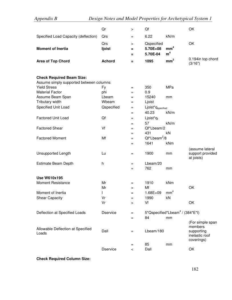
Appendix B Design Notes and Model Properties for Archetypical System 1
182
Qr > Qf
OK
Specified Load Capacity (deflection) Qrs = 6.22 kN/m
Qrs > Qspecified OK
Moment of Inertia Ijoist = 5.70E+08 mm4
= 5.70E-04 m
4
Area of Top Chord Achord = 1095 mm2
0.194in top chord (3/16")
Check Required Beam Size:
Assume simply supported between columns
Yield Stress Fy = 350 MPa
Material Factor phi = 0.9
Assume Beam Span Lbeam = 15240 mm
Tributary width Wbeam = Ljoist
Specified Unit Load Qspecified = Ljoist*qspecified
= 40.23 kN/m
Factored Unit Load Qf = Ljoist*qf
= 57 kN/m
Factored Shear Vf = Qf*Lbeam/2
= 431 kN
Factored Moment Mf = Qf*Lbeam
2/8
= 1641 kNm
Unsupported Length Lu = 1900 mm (assume lateral support provided at joists)
Estimate Beam Depth h = Lbeam/20
= 762 mm
Use W610x195
Moment Resistance Mr = 1910 kNm
Mr > Mf
OK
Moment of Inertia I = 1.68E+09 mm4
Shear Capacity Vr = 1990 kN
Vr > Vf
OK
Deflection at Specified Loads Dservice = 5*Qspecified*Lbeam
4 / (384*E*I)
= 84 mm
Allowable Deflection at Specified Loads
Dall = Lbeam/180
(For simple span members supporting inelastic roof coverings)
= 85 mm
Dservice < Dall
OK
Check Required Column Size:

Appendix B Design Notes and Model Properties for Archetypical System 1
183
Factored Axial Load Cf = 2*Vf
= 862 kN
Try HSS 254x254x9.5
Unbraced Length kLcolumn = h - joist depth
= 8.09 m
FactoredCompressive Resistance Cr = 1940 kN (CISCHandbook, pg 4-79)
Cr > Cf
OK
Base Shear Calculation (NBCC 2005):
For Diaphragm, assume: Rd = 1.5
Ro = 1.3
Building Period T = 0.05*h
3/4
= 0.26 s
T<2.0 seconds, and R=1.5, Therefire 2/3*S(0.2) cutoff applies
Spectral Acceleration S(0.2) = 0.94 g
= 100% of Vancouver Sa(0.2)
Soil Modification Factor Fa = 1.1 (Site Class D)
Importance Factor I = 1
Higher Mode Factor Mv = 1
Seismic Acceleration E = 0.66*I*S*Fa*Mv / (Rd*Ro)
= 0.35 g
= 0.68 g (for Rd, Ro = 1.0)
Unit Load on Roof Diaphragm Along Building Length
vroof = ((qroof+0.25*qsnow)*w + wc*t*h)*E
= 29 kN/m
Compare with Forces Due to wind
Wind Load (NBCC 2005 Cl 4.1.7) qwind = Iw*q*Ce*(Cp*Cg + Cpi*Cgi)
1 in 50 velocity pressure q = 0.48 kN/m2
Importance Factor Iw = 1
Exposure Factor Ce = 1
Exterior Gust Coeff Cp*Cg = 1.3 or -1.5
(positive denotes towards surface, neg denotes away)
Interior Pressure Coeff Cpi = 0.3 or -0.45
Interior Gust Coeff Cgi = 2
Inward pressure qwind inward = 1.0*q*1.0*(1.3 + 0.45*2.0)
Outward pressure qwind outward = 1.0*q*1.0*(-1.5 - 0.3*2.0)
Inward pressure governs
Design Wind Load qwind = 1.06 kN/m2
Unit Load on Roof Diaphragm Along Building Length
vwind = qwind*h*1.5
= 14 kN/m
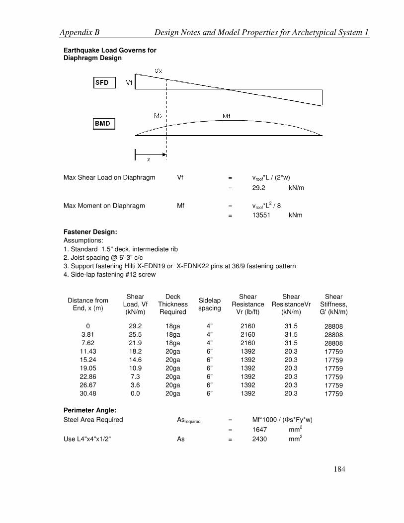
Appendix B Design Notes and Model Properties for Archetypical System 1
184
Earthquake Load Governs for Diaphragm Design
Max Shear Load on Diaphragm Vf = vroof*L / (2*w)
= 29.2 kN/m
Max Moment on Diaphragm Mf = vroof*L
2 / 8
= 13551 kNm
Fastener Design:
Assumptions:
1. Standard 1.5" deck, intermediate rib
2. Joist spacing @ 6'-3" c/c
3. Support fastening Hilti X-EDN19 or X-EDNK22 pins at 36/9 fastening pattern
4. Side-lap fastening #12 screw
Distance from End, x (m)
Shear Load, Vf (kN/m)
Deck Thickness Required
Sidelap spacing
Shear Resistance
Vr (lb/ft)
Shear ResistanceVr
(kN/m)
Shear Stiffness, G' (kN/m)
0 29.2 18ga 4" 2160 31.5 28808
3.81 25.5 18ga 4" 2160 31.5 28808
7.62 21.9 18ga 4" 2160 31.5 28808
11.43 18.2 20ga 6" 1392 20.3 17759
15.24 14.6 20ga 6" 1392 20.3 17759
19.05 10.9 20ga 6" 1392 20.3 17759
22.86 7.3 20ga 6" 1392 20.3 17759
26.67 3.6 20ga 6" 1392 20.3 17759
30.48 0.0 20ga 6" 1392 20.3 17759
Perimeter Angle:
Steel Area Required Asrequired = Mf*1000 / (Φs*Fy*w)
= 1647 mm
2
Use L4"x4"x1/2" As = 2430 mm
2
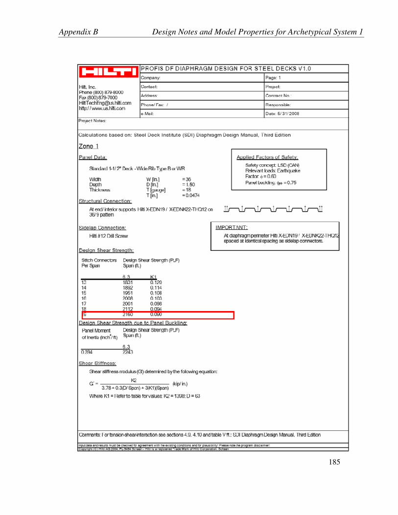
Appendix B Design Notes and Model Properties for Archetypical System 1
185

Appendix B Design Notes and Model Properties for Archetypical System 1
186
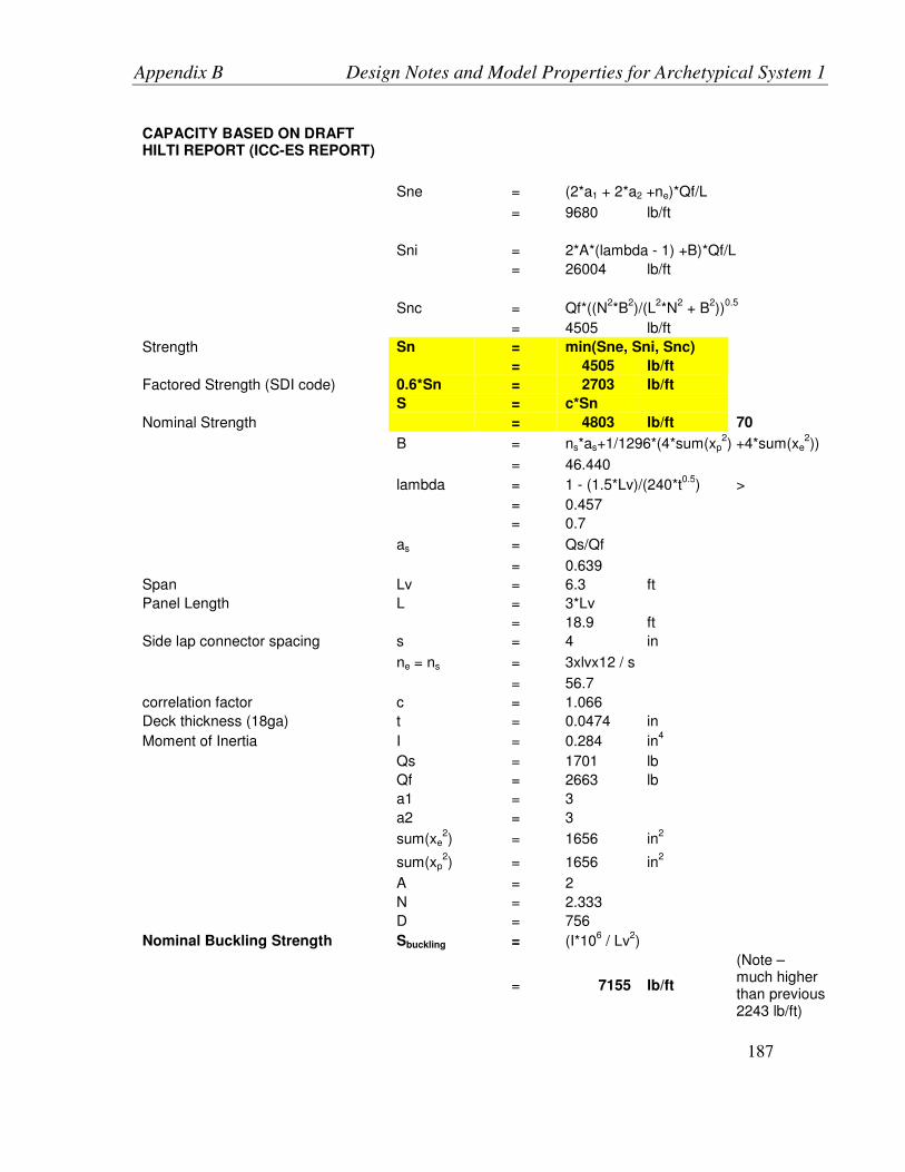
Appendix B Design Notes and Model Properties for Archetypical System 1
187
CAPACITY BASED ON DRAFT HILTI REPORT (ICC-ES REPORT)
Sne = (2*a1 + 2*a2 +ne)*Qf/L
= 9680 lb/ft
Sni = 2*A*(lambda - 1) +B)*Qf/L
= 26004 lb/ft
Snc = Qf*((N
2*B
2)/(L
2*N
2 + B
2))
0.5
= 4505 lb/ft
Strength Sn = min(Sne, Sni, Snc)
= 4505 lb/ft
Factored Strength (SDI code) 0.6*Sn = 2703 lb/ft
S = c*Sn
Nominal Strength = 4803 lb/ft 70
B = ns*as+1/1296*(4*sum(xp
2) +4*sum(xe
2))
= 46.440
lambda = 1 - (1.5*Lv)/(240*t
0.5) >
= 0.457
= 0.7
as = Qs/Qf
= 0.639
Span Lv = 6.3 ft
Panel Length L = 3*Lv
= 18.9 ft
Side lap connector spacing s = 4 in
ne = ns = 3xlvx12 / s
= 56.7
correlation factor c = 1.066
Deck thickness (18ga) t = 0.0474 in
Moment of Inertia I = 0.284 in
4
Qs = 1701 lb
Qf = 2663 lb
a1 = 3
a2 = 3
sum(xe
2) = 1656 in
2
sum(xp
2) = 1656 in
2
A = 2
N = 2.333
D = 756
Nominal Buckling Strength Sbuckling = (I*10
6 / Lv
2)
= 7155 lb/ft
(Note – much higher than previous 2243 lb/ft)

Appendix B Design Notes and Model Properties for Archetypical System 1
188
Notes:
The tables in the Hilti Report could not be included as they are confidential
The latest Hilti table provides different strength values for different base material thicknesses
In the original Hilti program, there was no distinction between different values for base material thickness
Using the SDI equations modified as per the latest Hilti Report, if a base material thickness smaller than 3/16 inch is used, the strength results are the same as provided by the Hilti software, however, if a base material thicker than 3/16 inch is used,
the strengths increase by about 25%
Factored Strength Nominal Strength
(lb/ft) (kN/m) (lb/ft) (kN/m)
Base material thickness < 3/16 inch
2127 31 4264 62
Base material thickness > 3/16 inch
2703 39 4802 70
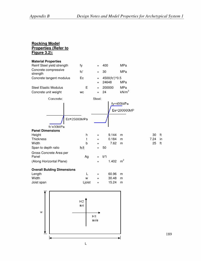
Appendix B Design Notes and Model Properties for Archetypical System 1
189
Rocking Model Properties (Refer to Figure 3.2):
Material Properties
Reinf Steel yield strength fy = 400 MPa
Concrete compressive strength
fc' = 30 MPa
Concrete tangent modulus Ec = 4500(fc')^0.5
= 24648 MPa
Steel Elastic Modulus E = 200000 MPa Concrete unit weight wc = 24 kN/m
3
Panel Dimensions
Height h = 9.144 m 30 ft
Thickness t = 0.184 m 7.24 in
Width b = 7.62 m 25 ft
Span to depth ratio h/t = 50
Gross Concrete Area per Panel Ag = b*t
(Along Horizontal Plane) = 1.402 m2
Overall Bulding Dimensions
Length L = 60.96 m
Width w = 30.48 m
Joist span Ljoist = 15.24 m

Appendix B Design Notes and Model Properties for Archetypical System 1
190
Dead Loads on Panel:
Roof Unit Load qroof = 1.0 kN/m2
Dead Load from tributary roof area
Wroof trib
= qroof*0.375*Ljoist*b
= 44 kN
Concrete Weight per panel Wp = wc*t*b*h
= 308 kN
Total Building Weight W = qroof*w*L + wc*t*2*(L+w)
= 9243 kN
Panel Reinforcement:
Vertical Reinforcement: 15M @ 400 alternating faces
Steel Steel Area As = 1000 mm2/m
Reinforcing Steel Ratio ρ = As/(1000*t*1000)
= 0.0054
Horizontal Reinforcement: 15M @ 400 alternating faces
Steel Steel Area As = 500 mm
2/m
Reinforcing Steel Ratio ρ = As/(1000*t*1000)
= 0.0027
Inelastic General Wall Element Properties
Mesh: n x n = 4x4 (Long Axis) 8x8 (End walls)
Vertical Concrete and Reinforcement Layer:
No. fibres required for steel = b / (n*bar spacing)
= b / (n*0.4m)
= 4.8 (use 5) 2.4 (use 3)
No. fibres for concrete = 4.8 (use 5) 2.4 (use 3)
Horizontal Concrete and Reinforcement Layer:
No. fibres required for steel = h/400/n
= 5.7 (use 6) 2.9 (use 3)
No. fibres for concrete = 5.7 (use 6) 2.9 (use 3)
Inelastic Shear Material:
Shear Strength (Paulay and Priestley - pg 127)
vy = 0.25*(fc')0.5
+ ρ*fy Based on Adebar et. al. (2004)
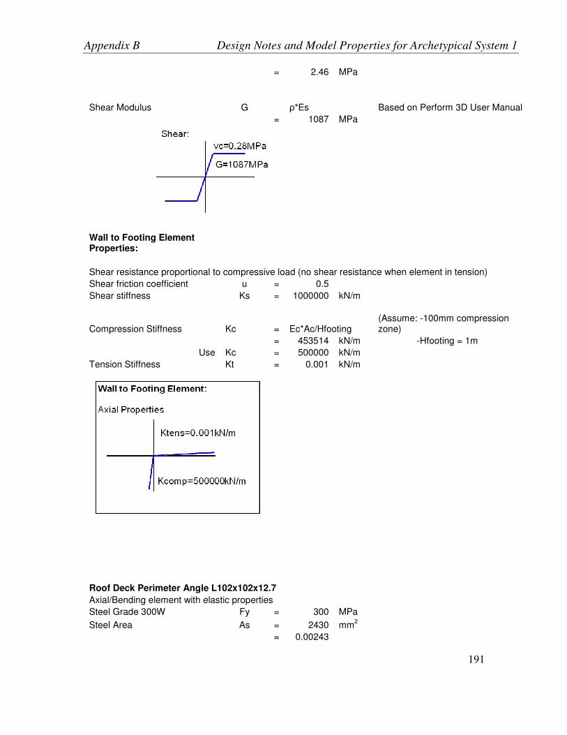
Appendix B Design Notes and Model Properties for Archetypical System 1
191
= 2.46 MPa
Shear Modulus G ρ*Es Based on Perform 3D User Manual
= 1087 MPa
Wall to Footing Element Properties:
Shear resistance proportional to compressive load (no shear resistance when element in tension)
Shear friction coefficient u = 0.5
Shear stiffness Ks = 1000000 kN/m
Compression Stiffness Kc = Ec*Ac/Hfooting (Assume: -100mm compression zone)
= 453514 kN/m -Hfooting = 1m
Use Kc = 500000 kN/m
Tension Stiffness Kt = 0.001 kN/m
Roof Deck Perimeter Angle L102x102x12.7
Axial/Bending element with elastic properties
Steel Grade 300W Fy = 300 MPa
Steel Area As = 2430 mm2
= 0.00243
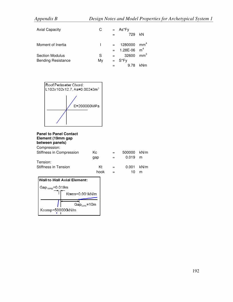
Appendix B Design Notes and Model Properties for Archetypical System 1
192
Axial Capacity C = As*Fy
= 729 kN
Moment of Inertia I = 1280000 mm4
= 1.28E-06 m4
Section Modulus S = 32600 mm3
Bending Resistance My = S*Fy
= 9.78 kNm
Panel to Panel Contact Element (19mm gap between panels)
Compression:
Stiffness in Compression Kc = 500000 kN/m
gap = 0.019 m
Tension:
Stiffness in Tension Kt = 0.001 kN/m
hook = 10 m
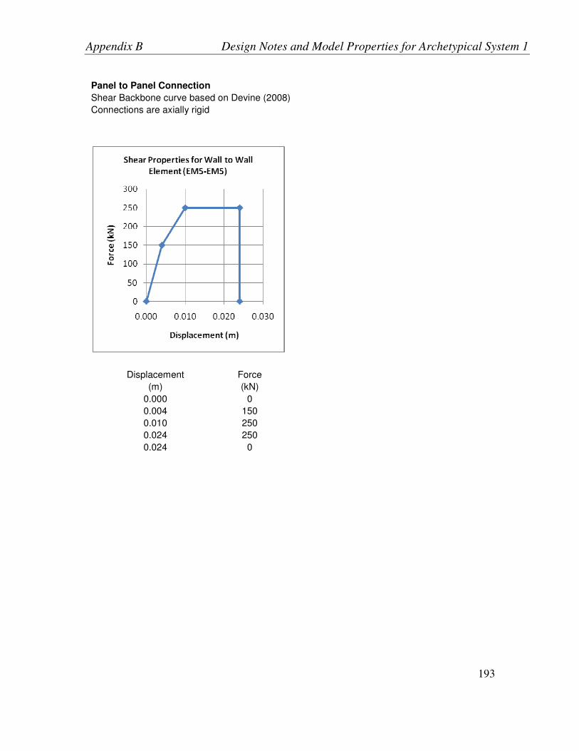
Appendix B Design Notes and Model Properties for Archetypical System 1
193
Panel to Panel Connection
Shear Backbone curve based on Devine (2008)
Connections are axially rigid
Displacement Force
(m) (kN)
0.000 0
0.004 150
0.010 250
0.024 250
0.024 0
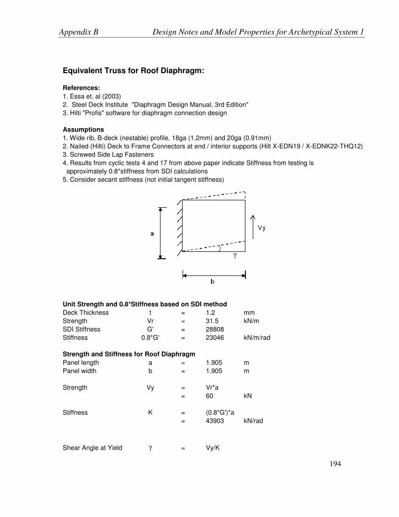
Appendix B Design Notes and Model Properties for Archetypical System 1
194
Equivalent Truss for Roof Diaphragm:
References:
1. Essa et. al (2003)
2. Steel Deck Institute "Diaphragm Design Manual, 3rd Edition"
3. Hilti "Profis" software for diaphragm connection design
Assumptions
1. Wide rib, B-deck (nestable) profile, 18ga (1.2mm) and 20ga (0.91mm)
2. Nailed (Hilti) Deck to Frame Connectors at end / interior supports (Hilt X-EDN19 / X-EDNK22-THQ12)
3. Screwed Side Lap Fasteners
4. Results from cyclic tests 4 and 17 from above paper indicate Stiffness from testing is
approximately 0.8*stiffness from SDI calculations
5. Consider secant stiffness (not initial tangent stiffness)
γ
Unit Strength and 0.8*Stiffness based on SDI method
Deck Thickness t = 1.2 mm
Strength Vr = 31.5 kN/m
SDI Stiffness G' = 28808
Stiffness 0.8*G' = 23046 kN/m/rad
Strength and Stiffness for Roof Diaphragm
Panel length a = 1.905 m
Panel width b = 1.905 m
Strength Vy = Vr*a
= 60 kN
Stiffness K = (0.8*G')*a
= 43903 kN/rad
Shear Angle at Yield γ = Vy/K
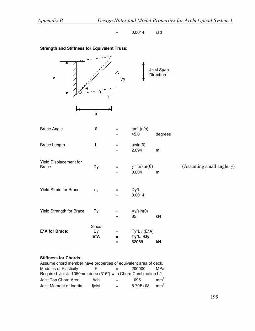
Appendix B Design Notes and Model Properties for Archetypical System 1
195
= 0.0014 rad
Strength and Stiffness for Equivalent Truss:
γ
Brace Angle θ = tan-1
(a/b)
= 45.0 degrees
Brace Length L = a/sin(θ)
= 2.694 m
Yield Displacement for Brace Dy = γ* b/sin(θ) (Assuming small angle, γ)
= 0.004 m
Yield Strain for Brace ey = Dy/L
= 0.0014
Yield Strength for Brace Ty = Vy/sin(θ)
= 85 kN
E*A for Brace: Since
Dy = Ty*L / (E*A)
E*A = Ty*L /Dy
= 62089 kN
Stiffness for Chords:
Assume chord member have properties of equivalent area of deck.
Modulus of Elasticity E = 200000 MPa
Required Joist: 1050mm deep (3'-6") with Chord Combination L/L
Joist Top Chord Area Ach = 1095 mm2
Joist Moment of Inertia Ijoist = 5.70E+08 mm4

Appendix B Design Notes and Model Properties for Archetypical System 1
196
= 0.0005698 m4
Parallel to Joists (perpendicular to flutes)
Area A2 = b*t/2 + Ach
= 0.00224 m2
Perpendicular to Joists (parallel to flutes)
A3 = a*t/2
= 0.00114 m2
Summary of Deck Equivalent Truss:
Deck Thickness Chord Area
Zone Gauge Thickness
(mm) Fastening
Pattern
Shear Resistance, Vr (kN/m)
Shear Stiffness
, G' (kN/m)
0.8*Shear Stiffness,
0.8*G' (kN/m)
E*A for Equivalent Brace (kN)
Perpendicular to Flutes (m
2)
Parallel to Flutes
(m2)
0 - 22.86m (75ft) from each end
18ga 1.204 36/9 31.5 28808 23046 62089 0.00224 0.00115
22.86m (75ft) to L/2 (150ft) from each end
20ga 0.909 36/9 20.3 17759 14207 38275 0.00196 0.00087
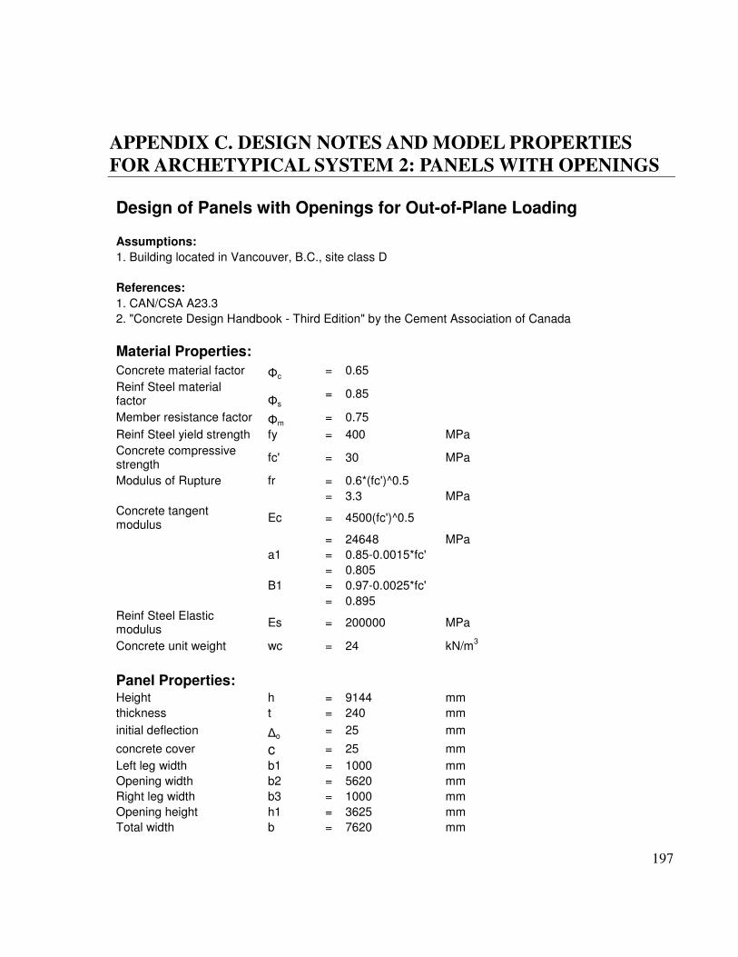
197
APPENDIX C. DESIGN NOTES AND MODEL PROPERTIES
FOR ARCHETYPICAL SYSTEM 2: PANELS WITH OPENINGS
Design of Panels with Openings for Out-of-Plane Loading
Assumptions:
1. Building located in Vancouver, B.C., site class D
References:
1. CAN/CSA A23.3
2. "Concrete Design Handbook - Third Edition" by the Cement Association of Canada
Material Properties:
Concrete material factor Φc = 0.65
Reinf Steel material factor Φs
= 0.85
Member resistance factor Φm = 0.75
Reinf Steel yield strength fy = 400 MPa
Concrete compressive strength
fc' = 30 MPa
Modulus of Rupture fr = 0.6*(fc')^0.5
= 3.3 MPa
Concrete tangent modulus
Ec = 4500(fc')^0.5
= 24648 MPa
a1 = 0.85-0.0015*fc'
= 0.805
B1 = 0.97-0.0025*fc'
= 0.895
Reinf Steel Elastic modulus
Es = 200000 MPa
Concrete unit weight wc = 24 kN/m3
Panel Properties:
Height h = 9144 mm
thickness t = 240 mm
initial deflection ∆o = 25 mm
concrete cover c = 25 mm
Left leg width b1 = 1000 mm
Opening width b2 = 5620 mm
Right leg width b3 = 1000 mm
Opening height h1 = 3625 mm
Total width b = 7620 mm

Appendix C Design Notes and Model Properties for Archetypical System 2
198
Loading:
Vertical Load Eccentricity ecc = t/2
= 120 mm
Roof Joist Span L = 15.24 m
Roof Joist Spacing s = 1.905 m
wall self weight qwall = wc*t
= 5.76 kN/m
2
Roof Self Wt. qroof = 1.0 kN/m
2
Snow Load (NBCC 2005 Cl
qsnow = Is*(Ss*(Cb*Cb*Cs*Ca)+Sr)
For tilt-up building in Vancouver:
Is = Ss = Cw = Cs = Ca = 1.0, Cb = 0.8
Ss = 1.8 kN/m
2
Sr = 0.2
Design Snow Load qsnow = 1.6 kN/m
2
Wind Load (NBCC 2005 Cl 4.1.7)
qwind = Iw*q*Ce*(Cp*Cg + Cpi*Cgi)
1 in 50 velocity pressure q = 0.48 kN/m2
Importance Factor Iw = 1
Exposure Factor Ce = 1
Exterior Gust Coeff Cp*Cg = 1.3 or -1.5 (positive denotes towards surface, neg denotes away)

Appendix C Design Notes and Model Properties for Archetypical System 2
199
Interior Pressure Coeff Cpi = 0.3 of -0.45
Interior Gust Coeff Cgi = 2
Inward pressure qwind
inward = 1.0*q*1.0*(1.3 + 0.45*2.0)
Outward pressure qwind
outward = 1.0*q*1.0*(-1.5 - 0.3*2.0)
Inward pressure governs
Design Wind Load qwind = 1.06 kN/m2
Eccentricity ecc = t/2
= 4572 mm
Seismic for Out-of-Plane forces (NBCC 2005 Cl 4.1.8.17)
Vp = 0.3*Fa*Sa(0.2)*Ie*Sp*Wp
Soil Modification Factor Fa = 1.1
(For Site Class D)
Spectral Acceleration at T=0.2s
Sa(0.2) = 0.94 g
Importance Factor Ie = 1.0
Sp = Cp*Ar*Ax / Rp
where 0.7<Sp<4.0
Component Risk Factor Cp = 1.0
Dynamic Amplification Factor
Ar = 1.0
(Typically used for tilt-up but maybe unconservative)
Height Factor Ax = 1+ 2*hx/hn
hx = Height of component above base
= Centre of mass of panel
hn = total height
Ax = 2
Response Factor Rp = 2.5
(for reinforced tilt-up wall panels)
Sp = 0.8
Seismic for Out-of-Plane forces
Vp = 0.248 *Wp
Compare Seismic to Wind (for 1m unit strip)
Factored Seismic out-of-plane
qseismic = Vp*1.0m*qwall
= 1.43 kN/m
Factored Wind 1.5*qwind = 1.58 kN/m
Wind Governs for Out-of-Plane Loading on Panels
Strength Calculations:
Load Case (4): 1.25D + 1.4W + 0.5S
Right Leg
Tributary panel width bt3 = b3+b2/2
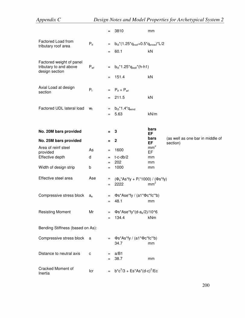
Appendix C Design Notes and Model Properties for Archetypical System 2
200
= 3810 mm
Factored Load from tributary roof area
Ptf = bt3*(1.25*qroof+0.5*qsnow)*L/2
= 60.1 kN
Factored weight of panel tributary to and above design section
Pwf = bt3*1.25*qwall*(h-h1)
= 151.4 kN
Axial Load at design section
Pf = Ptf + Pwf
= 211.5 kN
Factored UDL lateral load wf = bt3*1.4*qwind
= 5.63 kN/m
No. 20M bars provided
= 3 bars EF
No. 25M bars provided
= 2 bars EF
(as well as one bar in middle of section)
Area of reinf steel provided
As = 1600 mm
2
EF
Effective depth d = t-c-db/2 mm
= 202 mm
Width of design strip b = 1000 mm
Effective steel area Ase = (Φs*As*fy + Pf*1000) / (Φs*fy)
= 2222 mm
2
Compressive stress block ae = Φs*Ase*fy / (a1*Φc*fc'*b)
= 48.1 mm
Resisting Moment Mr = Φs*Ase*fy*(d-ae/2)/10^6
= 134.4 kNm
Bending Stiffness (based on As):
Compressive stress block a = Φs*As*fy / (a1*Φc*fc'*b)
34.7 mm
Distance to neutral axis c = a/B1
= 38.7 mm
Cracked Moment of Inertia
Icr = b*c3/3 + Es*As*(d-c)
2/Ec

Appendix C Design Notes and Model Properties for Archetypical System 2
201
= 3.65E+08 mm
4/m
Kbf = 48*Ec*Icr / 5*h
2*1000
= 1034.3 kNm/m
Moment Magnifier δb = 1/(1-Pf/(Φm*Kbf))
= 1.37
Max out-of-plane shear due to wind
Vwind = wf*h/2
Primary Bending Moment Mb = (wf*h1)*(h-h1)/2 + Ptf*ecc/2 + Pf*∆o
= 65.2 kNm
Total Moment Mf = δb*Mb
= 89.7 kNm
Mf < Mr
OK
89.7
134.4 kNm
Total factored deflection ∆f = Mf / (Φm*Kbf)
= 116 mm
Check for maximum reinforcement
Total steel area As = 4800
As/(b*d) < a1*B1*Φc*fc'*700/ (Φs*fy*(700+fy))
0.0238 < 0.026
OK
Deflections at Service Loads for Leg
Load Case: 1.0D + 1.0W + 0.5S (Iw = 0.75, Is = 0.9)
Panel width b = 1000 mm
Tributary panel width bt3 = 3810 mm
Factored Load from tributary roof area
Pts = bt3*(1.0*qroof+0.5*0.9*qsnow)*L/2
= 50.5 kN
Factored weight of panel tributary to and above design section
Pws = bt3*1.0*qwall*h1
= 79.6 kN

Appendix C Design Notes and Model Properties for Archetypical System 2
202
Axial Load at mid-height Ps = Ptf + Pwf
= 130.0 kN
Service UDL lateral load ws = bt3*1.0*lw*qwind
= 3.02 kN/m
Gross Moment of Inertia Ig = b*1000*t
3/12
= 1152000000 mm
4
N.A. to extreme fibre yt = t/2
120 mm
Cracking Moment Mcr = fr*Ig/yt
= 31.55 kNm
Primary Bending Moment Mbs = ws*h1*(h-h1)/2 + Pts*ecc/2 + Ps*∆o
= 36.46 kNm
Using a triangular concrete stress distribution
n = Es/Ec
= 8.1
kd = (-n*As + ((n*As)^2 + 2*b*n*As*d)^0.5)/b
= 60.6 mm
Icr = b*(kd)^3/3 + n*As*(kd - d)^2
= 333764316.7 mm
4
Initially assume ∆s = h/100
= 91.4 mm
Ms = Mbs + Ps*∆s
= 48.4 kNm
Effective Moment of Inertia
Ie = Icr + (Ig - Icr)*(Mcr/Ms)^3
= 561074094.0 mm
4
Stiffness Kbs = 48*Ec*Ie / 5*h
2*1000
= 1588 kNm/m
Moment Magnifier δb = 1/(1-Ps/Kbs)
= 1.09
Total Moment Ms = δb*Mbs

Appendix C Design Notes and Model Properties for Archetypical System 2
203
= 39.7 kNm
Ms < Mr
OK
39.7
48.4 kNm
max service deflection ∆s = Ms/Kbs*1000
= 25.0 mm
∆s < ∆si
OK

Appendix C Design Notes and Model Properties for Archetypical System 2
204
Design of Panels with Openings for In-Plane Loading
Assumptions:
1. Building located in Vancouver, B.C., site class D
References:
1. CAN/CSA A23.3
2. "Concrete Design Handbook - Third Edition" by the Cement Association of Canada
Material Properties: Concrete material factor Φc = 0.65
Reinf Steel material factor Φs = 0.85
Member resistance factor Φm = 0.75
Reinf Steel yield strength fy = 400 MPa
Concrete compressive strength
fc' = 30 MPa
Modulus of Rupture fr = 0.6*(fc')^0.5
= 3.3 MPa
Concrete tangent modulus Ec = 4500(fc')^0.5
= 24648 MPa
a1 =
0.85-0.0015*fc'
= 0.805
B1 =
0.97-0.0025*fc'
= 0.895
Reinf Steel Elastic modulus Es = 200000 MPa
Concrete unit weight wc = 24 kN/m3
Friction Coeff at Base µ = 0.5
Max concrete strain ec = 0.0035
Panel Layout:
Leg thickness of 240mm required for out-of-plane loading
Minimum 4:1 width/thickness ratio required, so width minimum 960mm. 1000mm selected
To maintain same aspect ratio as test panel, leg height increased to 3625mm
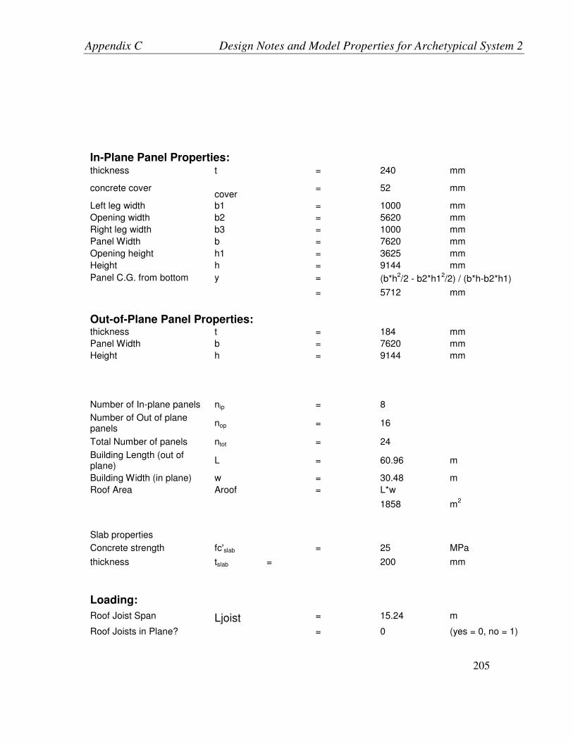
Appendix C Design Notes and Model Properties for Archetypical System 2
205
In-Plane Panel Properties:
thickness t = 240 mm
concrete cover cover
= 52 mm
Left leg width b1 = 1000 mm
Opening width b2 = 5620 mm
Right leg width b3 = 1000 mm
Panel Width b = 7620 mm
Opening height h1 = 3625 mm
Height h = 9144 mm
Panel C.G. from bottom y = (b*h2/2 - b2*h1
2/2) / (b*h-b2*h1)
= 5712 mm
Out-of-Plane Panel Properties:
thickness t = 184 mm
Panel Width b = 7620 mm
Height h = 9144 mm
Number of In-plane panels nip = 8
Number of Out of plane panels
nop = 16
Total Number of panels ntot = 24
Building Length (out of plane)
L = 60.96 m
Building Width (in plane) w = 30.48 m
Roof Area Aroof = L*w
1858 m
2
Slab properties
Concrete strength fc'slab = 25 MPa
thickness tslab = 200 mm
Loading:
Roof Joist Span Ljoist = 15.24 m
Roof Joists in Plane? = 0 (yes = 0, no = 1)

Appendix C Design Notes and Model Properties for Archetypical System 2
206
wall self weight qwall = wc*t
= 5.76 kN/m
2
Roof Self Wt. qroof = 1.0 kN/m
2
Snow Load qsnow = Is*(Ss*(Cb*Cb*Cs*Ca)+Sr)
For tilt-up building in Vancouver:
Is = Ss = Cw = Cs = Ca = 1.0, Cb = 0.8
Ss = 1.8 kN/m2
Sr = 0.2
qsnow = 1.6 kN/m
2
Roof Weight per panel Wr = qroof*b*Ljoist/2
= 0
kN/panel (No roof weight if joists spanning in plane)
Panel with opening Weight Wpo = qwall*(b*h - b2*h1)
= 284 kN/panel
Solid Panel Weight Wps = wc*t*b*h
= 308 kN/panel
Total Building Weight W = qroof*Aroof + nip*Wpo + nop*Wps
= 9053 kN (Calculated)
= 9010 kN
(From Perform)
Base Shear Calculation for Rd, Ro = 1.0 (NBCC 2005)
Building Period T = 0.05*h
3/4
= 0.26 s
T<2.0 seconds, and R=1.5, Therefore 2/3*S(0.2) applies
Spectral Acceleration S(0.2) = 0.94 g
Soil Modification Factor Fa = 1.1
Importance Factor I = 1.0
Higher Mode Factor Mv = 1
Seismic Load E = 0.66*I*S*Fa*Mv / (Rd*Ro)
= 0.68 g
Force from Roof Diaphram Vroof = ((qroof+0.25*qsnow)*Aroof + Wps*nop*0.5)*E*0.5
= 1734 kN per one wall line
Shear from in-plane panels Vpanels = E*nip*Wpo*0.5
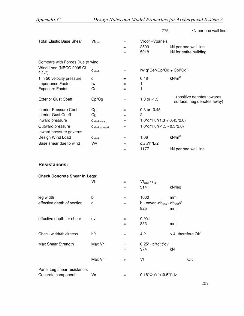
Appendix C Design Notes and Model Properties for Archetypical System 2
207
775 kN per one wall line
Total Elastic Base Shear Vftotal = Vroof +Vpanels
= 2509 kN per one wall line
= 5018 kN for entire building
Compare with Forces Due to wind
Wind Load (NBCC 2005 Cl 4.1.7)
qwind = Iw*q*Ce*(Cp*Cg + Cpi*Cgi)
1 in 50 velocity pressure q = 0.48 kN/m2
Importance Factor Iw = 1
Exposure Factor Ce = 1
Exterior Gust Coeff Cp*Cg = 1.3 or -1.5 (positive denotes towards
surface, neg denotes away)
Interior Pressure Coeff Cpi = 0.3 or -0.45
Interior Gust Coeff Cgi = 2
Inward pressure qwind inward = 1.0*q*1.0*(1.3 + 0.45*2.0)
Outward pressure qwind outward = 1.0*q*1.0*(-1.5 - 0.3*2.0)
Inward pressure governs
Design Wind Load qwind = 1.06 kN/m2
Base shear due to wind Vw = qwind*h*L/2
= 1177 kN per one wall line
Resistances:
Check Concrete Shear in Legs:
Vf = Vftotal / nip
= 314 kN/leg
leg width b = 1000 mm
effective depth of section d = b - cover -dbties - dbvert/2
925 mm
effective depth for shear dv = 0.9*d
= 833 mm
Check width/thickness h/t = 4.2 > 4, therefore OK
Max Shear Strength Max Vr = 0.25*Φc*fc'*t*dv
= 974 kN
Max Vr > Vf
OK
Panel Leg shear resistance:
Concrete component Vc = 0.18*Φc*(fc')0.5*t*dv
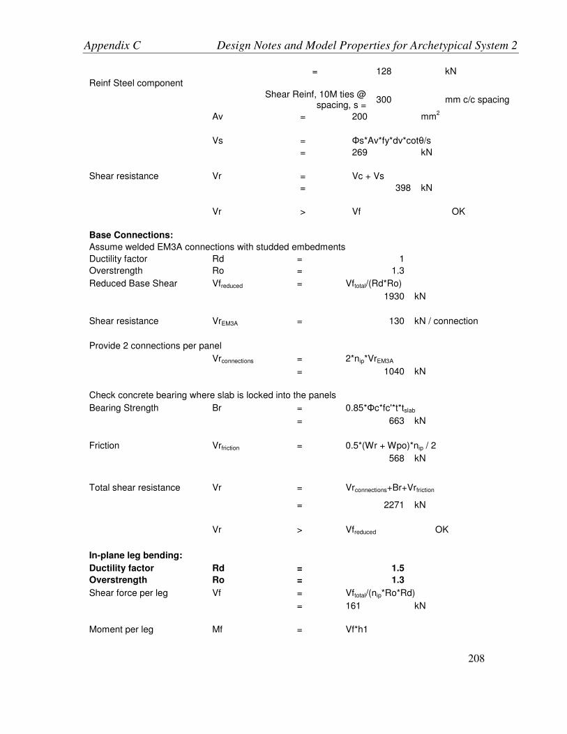
Appendix C Design Notes and Model Properties for Archetypical System 2
208
= 128 kN
Reinf Steel component
Shear Reinf, 10M ties @
spacing, s = 300 mm c/c spacing
Av = 200 mm2
Vs = Φs*Av*fy*dv*cotθ/s
= 269 kN
Shear resistance Vr = Vc + Vs
= 398 kN
Vr > Vf
OK
Base Connections:
Assume welded EM3A connections with studded embedments
Ductility factor Rd = 1
Overstrength Ro = 1.3
Reduced Base Shear Vfreduced = Vftotal/(Rd*Ro)
1930 kN
Shear resistance VrEM3A = 130 kN / connection
Provide 2 connections per panel
Vrconnections = 2*nip*VrEM3A
= 1040 kN
Check concrete bearing where slab is locked into the panels
Bearing Strength Br = 0.85*Φc*fc'*t*tslab
= 663 kN
Friction Vrfriction = 0.5*(Wr + Wpo)*nip / 2
568 kN
Total shear resistance Vr = Vrconnections+Br+Vrfriction
= 2271 kN
Vr > Vfreduced OK
In-plane leg bending:
Ductility factor Rd = 1.5
Overstrength Ro = 1.3
Shear force per leg Vf = Vftotal/(nip*Ro*Rd)
= 161 kN
Moment per leg Mf = Vf*h1

Appendix C Design Notes and Model Properties for Archetypical System 2
209
= 583 kNm
No. of 25M Vertical Reinforcing Bars = 6 bars
No. of 20M Vertical Reinforcing Bars = 6 bars
Total Steel Area Provided Astot = 4800 mm
2
Steel Area for Bending As = 2700 mm
2
Effective Depth if assume bottom three rows in compression:
Number of rows of bars: 5
Bar diameter: 25 mm
Row No. Distance
from Bottom
Steel Area (mm2)
1 75 1500
2 287 600
3 500 600
4 713 600
5 926 1500
Distance to centroid of steel area from bottom
y = Sum(Ai*di) / Sum(Ai)
216 mm
Effective Depth:
d = b-y
d = 784 mm
Compression block a = Φs*fy*As/(Φc*fc'*a1*t)
= 244 mm
Check neutral axis c = a/B1
= 272 mm
check max rebar strain es = ec/c*(b1-c-cover-stirrup)
= 0.009 < 0.05 OK
Moment Resistance Mr = Φs*fy*As*(d-a/2)
= 608 kNm
Mr > Mf
OK
Lateral resistance Vrleg = Mr/h1
= 168 kN
Nominal lateral resistance Vrleg/Φc = 258 kN
Tie spacing in Hinge region s = 8*dbvert
= 200 mm
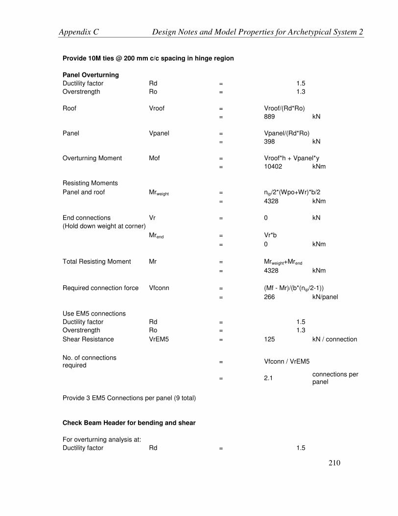
Appendix C Design Notes and Model Properties for Archetypical System 2
210
Provide 10M ties @ 200 mm c/c spacing in hinge region
Panel Overturning
Ductility factor Rd = 1.5
Overstrength Ro = 1.3
Roof Vroof = Vroof/(Rd*Ro)
= 889 kN
Panel Vpanel = Vpanel/(Rd*Ro)
= 398 kN
Overturning Moment Mof = Vroof*h + Vpanel*y
= 10402 kNm
Resisting Moments
Panel and roof Mrweight = nip/2*(Wpo+Wr)*b/2
= 4328 kNm
End connections Vr = 0 kN
(Hold down weight at corner)
Mrend = Vr*b
= 0 kNm
Total Resisting Moment Mr = Mrweight+Mrend
= 4328 kNm
Required connection force Vfconn = (Mf - Mr)/(b*(nip/2-1))
= 266 kN/panel
Use EM5 connections
Ductility factor Rd = 1.5
Overstrength Ro = 1.3
Shear Resistance VrEM5 = 125 kN / connection
No. of connections required
= Vfconn / VrEM5
= 2.1
connections per panel
Provide 3 EM5 Connections per panel (9 total)
Check Beam Header for bending and shear
For overturning analysis at:
Ductility factor Rd = 1.5

Appendix C Design Notes and Model Properties for Archetypical System 2
211
Overstrength Ro = 1.3
Maximum Shear force Vf = Vfconn+Wr/2+Wpo/2
= 408 kN
Horizontal distance from end to C.G. for half panel
x = h*b12/2+(h-h1)*(b2/2)*(b/2-b2/4) / (h*b1+(h-h1)*(b2/2))
= 1698 mm
Maximum Moment Mf = Vf*b/2 + (Wr/2)*b/4 + (Wpo/2)*x -
Vroofp3*h/(2*nip/2*Rd*Ro) - Vpanel*y/(2*nip/2*Rd*Ro)
= 494 kNm
section width b = h-h1
= 5519 mm
effective depth d = b - cover -dbhor - dbvert/2
= 5444 mm
Steel Area (assume 2 - 20M bars are engaged)
As = 600 mm2
Compression block a = Φs*fy*As/(Φc*fc'*a1*t)
= 54 mm
Moment Resistance Mr = Φs*fy*As*(d-a/2)
= 1105 kNm
Mr > Mf
OK
Check for potential yielding of longitudinal reinforcement
Multiply moment by Rd = 1.5
Ro = 1.3
Maximum Moment Mf = 964 kNm
Mr > Mf
Reinforcing will not yield and anti-buckling ties not required
Use 10M @ 400 EW As = 500 mm
2/m
Minimum Reinforcing Asmin = 0.002*Ag
= 480 mm2/m

Appendix C Design Notes and Model Properties for Archetypical System 2
212
As > Asmin OK
Check Shear in Header
Multiply moment by Rd = 1.5
Ro = 1.3
Maximum Shear Force Vf = 795 kN
Effective depth for shear dv = 0.9*d
= 4900 mm
Concrete component Vc = 0.18*Φc*(fc')0.5*t*dv
= 754 kN
Reinf Steel component
Shear Reinf, 10M ties @
spacing, s = 400 mm c/c spacing
Av = 200 mm2
Vs = Φs*Av*fy*dv*cotθ/s
= 1190 kN
Shear resistance Vr = Vc + Vs
= 1943 kN
Vr > Vf
OK
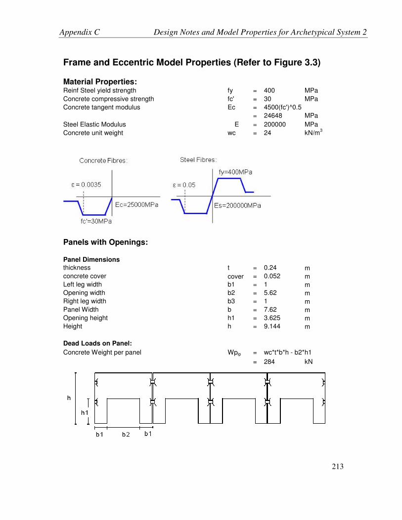
Appendix C Design Notes and Model Properties for Archetypical System 2
213
Frame and Eccentric Model Properties (Refer to Figure 3.3)
Material Properties: Reinf Steel yield strength fy = 400 MPa
Concrete compressive strength fc' = 30 MPa
Concrete tangent modulus Ec = 4500(fc')^0.5
= 24648 MPa
Steel Elastic Modulus E = 200000 MPa
Concrete unit weight wc = 24 kN/m3
Panels with Openings:
Panel Dimensions
thickness t = 0.24 m
concrete cover cover = 0.052 m
Left leg width b1 = 1 m
Opening width b2 = 5.62 m
Right leg width b3 = 1 m
Panel Width b = 7.62 m
Opening height h1 = 3.625 m
Height h = 9.144 m
Dead Loads on Panel:
Concrete Weight per panel Wpip = wc*t*b*h - b2*h1
= 284 kN

Appendix C Design Notes and Model Properties for Archetypical System 2
214
Leg Vertical Reinforcement:
No. 25M bars 6
No. 20M bars 6
Steel Steel Area As = 4800 mm
2
Reinforcing Steel Ratio ρ = As/(b1*t)
= 0.0200
Hinge Zone
Horizontal Reinforcement: 10M @ 200 each face
Steel Steel Area As = 1000 mm2/m
Reinforcing Steel Ratio ρ = As/(1000*t*1000)
= 0.0042
Inelastic General Wall Element Properties
Mesh: n x n = 2x4
Vertical Concrete and Reinforcement Layer:
No. fibres required for steel = No. vertical bars /2
= 6.0
No. fibres for concrete = 6.0
Horizontal Concrete and Reinforcement Layer:
No. fibres required for steel = h1/200/n
= 4.5 (use 6)
No. fibres for concrete = 4.5 (use 6)
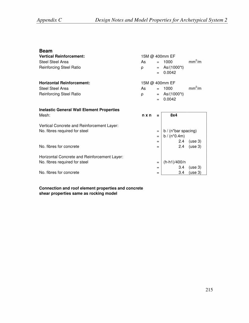
Appendix C Design Notes and Model Properties for Archetypical System 2
215
Beam Vertical Reinforcement: 15M @ 400mm EF
Steel Steel Area As = 1000 mm
2/m
Reinforcing Steel Ratio ρ = As/(1000*t)
= 0.0042
Horizontal Reinforcement: 15M @ 400mm EF
Steel Steel Area As = 1000 mm2/m
Reinforcing Steel Ratio ρ = As/(1000*t)
= 0.0042
Inelastic General Wall Element Properties
Mesh: n x n = 8x4
Vertical Concrete and Reinforcement Layer:
No. fibres required for steel = b / (n*bar spacing)
= b / (n*0.4m)
= 2.4 (use 3)
No. fibres for concrete = 2.4 (use 3)
Horizontal Concrete and Reinforcement Layer:
No. fibres required for steel = (h-h1)/400/n
= 3.4 (use 3)
No. fibres for concrete = 3.4 (use 3)
Connection and roof element properties and concrete
shear properties same as rocking model
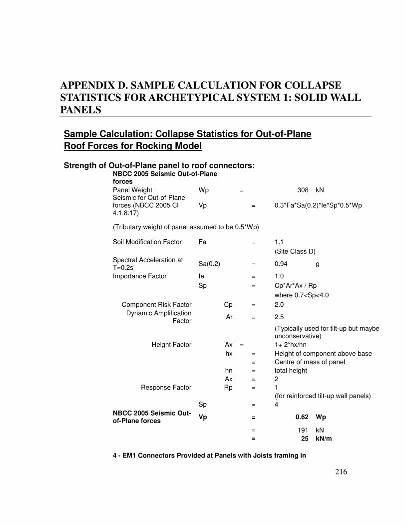
Appendix D Sample Calculation for Collapse Statistics
216
APPENDIX D. SAMPLE CALCULATION FOR COLLAPSE
STATISTICS FOR ARCHETYPICAL SYSTEM 1: SOLID WALL
PANELS
Sample Calculation: Collapse Statistics for Out-of-Plane
Roof Forces for Rocking Model
Strength of Out-of-Plane panel to roof connectors: NBCC 2005 Seismic Out-of-Plane forces
Panel Weight Wp = 308 kN Seismic for Out-of-Plane forces (NBCC 2005 Cl 4.1.8.17)
Vp = 0.3*Fa*Sa(0.2)*Ie*Sp*0.5*Wp
(Tributary weight of panel assumed to be 0.5*Wp)
Soil Modification Factor Fa = 1.1
(Site Class D)
Spectral Acceleration at T=0.2s
Sa(0.2) = 0.94 g
Importance Factor Ie = 1.0
Sp = Cp*Ar*Ax / Rp
where 0.7<Sp<4.0
Component Risk Factor Cp = 2.0
Dynamic Amplification Factor
Ar = 2.5
(Typically used for tilt-up but maybe unconservative)
Height Factor Ax = 1+ 2*hx/hn
hx = Height of component above base
= Centre of mass of panel
hn = total height
Ax = 2
Response Factor Rp = 1
(for reinforced tilt-up wall panels)
Sp = 4
NBCC 2005 Seismic Out-of-Plane forces
Vp = 0.62 Wp
= 191 kN
= 25 kN/m
4 - EM1 Connectors Provided at Panels with Joists framing in

Appendix D Sample Calculation for Collapse Statistics
217
Design Strength tr = 70 kN/connector
for wall thickness > 150mm
Total strength Tr = 280 kN / 4 connectors
Nominal strength tult = tr/0.6
= 117 kN/connector
= 467 kN / 4 connectors
Nominal strength per unit length = 61 kN/m
At panels without joists, consider nominal strength = NBCC 2005 forces / 0.6
(Testing by Lemieux et. al, 1998, considered the design strength of standard embedded
connectors to be 0.6*mean strength)
Nominal strength per unit length = 42 kN/m
Consider the following IDA results for Rocking Model Out-of-Plane Panel to Roof Forces:
Sa(T1)
Earthquake Record Sa(T1) = 0 0.5g 1.0g 2.0g
Sa(T1) at
(1)
Capacity
MUL009 0 13 34 68 1.227
L0S000 0 22 43 46 0.972
BOL000 0 18 33 39 2.505
HEC000 0 16 41 66 1.032
H-DLT262 0 17 46 73 0.932
H-E11140 0 41 65 86 0.527
NIS000 0 16 35 67 1.223
SHI000 0 20 62 69 0.763
DZC180 0 16 33 55 1.422
ARC000 0 19 42 62 0.996
YER270 0 12 63 78 0.795
CLW-LN 0 13 30 69 1.301
CAP000 0 49 84 98 0.428
GO3000 0 51 72 101 0.411
ABBAR-L 0 58 88 107 0.364
B-ICC000 0 18 38 35 Not
exceeded
B-POE270 0 14 32 64 1.308
RIO270 0 21 53 63 0.834
CHY101-E 0 19 59 81 0.792
TCU045-E 0 16 38 46 1.502
PEL090 0 20 53 76 0.832
A-TMZ000 0 14 27 61 1.440

Appendix D Sample Calculation for Collapse Statistics
218
MEDIAN 0 18 43 68 0.986
Note that the Sa(T1) at capacity was determined by linear interpolation between the two IDA data points
lesser and greater than than capacity
The table below shows the IDA data sorted by increasing Sa(T1) (1)
The P[Collapse based on the raw data is calculated by dividing the number of the record
in sequence from smallest Sa(T1) to largest divided by the total number of records
Record No. Eq Record
Sa(T1) at which drift
criteria exceeded
(g) ln(Sa(T1)
Raw Data
(1)
P[Collapse]
0.00 0.00
1 ABBAR-L 0.364 -1.01 0.05
2 GO3000 0.411 -0.89 0.10
3 CAP000 0.428 -0.85 0.14
4 H-E11140 0.527 -0.64 0.19
5 SHI000 0.763 -0.27 0.24
6 CHY101-E 0.792 -0.23 0.29
7 YER270 0.795 -0.23 0.33
8 PEL090 0.832 -0.18 0.38
9 RIO270 0.834 -0.18 0.43
10 H-DLT262 0.932 -0.07 0.48
11 L0S000 0.972 -0.03 0.52
12 ARC000 0.996 0.00 0.57
13 HEC000 1.032 0.03 0.62
14 NIS000 1.223 0.20 0.67
15 MUL009 1.227 0.20 0.71
16 CLW-LN 1.301 0.26 0.76
17 B-POE270 1.308 0.27 0.81
18 DZC180 1.422 0.35 0.86
19 A-TMZ000 1.440 0.36 0.90
20 TCU045-E 1.502 0.41 0.95
21 BOL000 2.505 0.92 1.00
Median 0.972 Mean, µ = LN(Median Sa(T1))
-0.03
Std Dev of LN(Sa(T1))
0.48
Sources of Uncertainty (Based on ATC-63 Methodology):
Record to Record Collapse Uncertainty, BRTR = 0.48
(Same as standard deviation above)
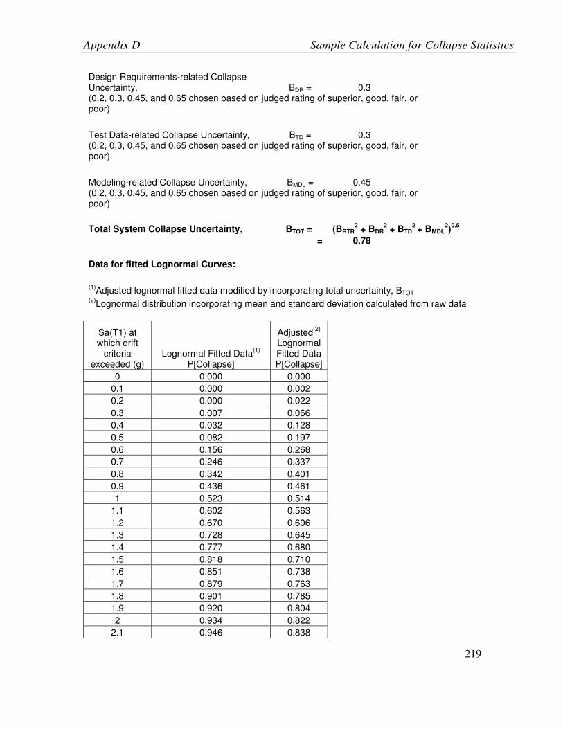
Appendix D Sample Calculation for Collapse Statistics
219
Design Requirements-related Collapse Uncertainty, BDR = 0.3 (0.2, 0.3, 0.45, and 0.65 chosen based on judged rating of superior, good, fair, or poor)
Test Data-related Collapse Uncertainty, BTD = 0.3 (0.2, 0.3, 0.45, and 0.65 chosen based on judged rating of superior, good, fair, or poor)
Modeling-related Collapse Uncertainty, BMDL = 0.45 (0.2, 0.3, 0.45, and 0.65 chosen based on judged rating of superior, good, fair, or poor)
Total System Collapse Uncertainty, BTOT = (BRTR2 + BDR
2 + BTD
2 + BMDL
2)0.5
= 0.78
Data for fitted Lognormal Curves:
(1)Adjusted lognormal fitted data modified by incorporating total uncertainty, BTOT
(2)Lognormal distribution incorporating mean and standard deviation calculated from raw data
Sa(T1) at which drift
criteria exceeded (g)
Lognormal Fitted Data(1)
P[Collapse]
Adjusted(2)
Lognormal Fitted Data P[Collapse]
0 0.000 0.000
0.1 0.000 0.002
0.2 0.000 0.022
0.3 0.007 0.066
0.4 0.032 0.128
0.5 0.082 0.197
0.6 0.156 0.268
0.7 0.246 0.337
0.8 0.342 0.401
0.9 0.436 0.461
1 0.523 0.514
1.1 0.602 0.563
1.2 0.670 0.606
1.3 0.728 0.645
1.4 0.777 0.680
1.5 0.818 0.710
1.6 0.851 0.738
1.7 0.879 0.763
1.8 0.901 0.785
1.9 0.920 0.804
2 0.934 0.822
2.1 0.946 0.838

Appendix D Sample Calculation for Collapse Statistics
220
2.2 0.956 0.852
2.3 0.964 0.865
2.4 0.971 0.876
2.5 0.976 0.887
2.6 0.980 0.896
2.7 0.984 0.904
2.8 0.987 0.912
2.9 0.989 0.919
3 0.991 0.925
3.1 0.992 0.931
3.2 0.994 0.936
3.3 0.995 0.941
3.4 0.996 0.945
3.5 0.996 0.949
3.6 0.997 0.953
3.7 0.997 0.956
3.8 0.998 0.959
3.9 0.998 0.962
4 0.998 0.965
Sa(T1) for which less than 10% of structures will fail, Sa(T1)10%: 0.36g
(for lognormal fitted data with adjustment for uncertainty):
This value is obtained by either interpolating from the adjusted lognormal distribution
data above or by using the solver function - changing the Sa(T1) value such that the adjusted
lognormal cumulative distribution is equal to 0.1, i.e. LOGNORMDIST(Sa(T1),µ,BTOT) = 0.1
Compare with Design Base Shear:
1 in 2475 Base Shear for Vancouver (Including 1/3 reduction), Sa(T1)des = 0.68g
So for the current R value used, the out-of-plane wall to roof connections are overstressed by 0.68/0.36 = 1.89 or 89%

Appendix D Sample Calculation for Collapse Statistics
221
Figure D1: Collapse Statistics for Out-of-Plane Deck Forces: