Analog-VLSI, Array-Processor Based, Bayesian, Multi-Scale Optical Flow

Estimation

L. Torok, A. Zarandy

Analogic and Neural Computing Systems Laboratory,

Computer and Automation Research Institute

Hungarian Academy of Sciences, H-1111, Budapest,

Kende u. 13-17, Hungary, e-mail: torok,zarandy@sztaki.hu

November 10, 2005

Abstract

Optical flow (OF) estimation aims at derive a motion-vector field that characterizes motions on a video sequence

of images. In this paper we propose a new multi-scale (or scale-space) algorithm that generates OF on Cellular

Neural/Non-linear Network Universal Machine (CNN-UM), a general purpose analog-VLSI hardware, at resolution

of 128x128 with fair accuracy and working over a speed of 100 frames per second. The performance of the hardware

implementation of the proposed algorithm is measured on a standard image sequence. As far as we are concerned,

this is the first time when an OF estimator hardware is tested on a practical-size standard image sequence.

Keywords: Multi-scale, Optical Flow Algorithm, Analog VLSI Implementation, Cellular Neural/Non-linear

Network

1 Introduction

In general, a visual sensory system (VSS) can be interpreted as a system that records light in a 2 dimensional (image)

plane reflected by illuminated, 3 dimensional, real-world objects. The objects of the environment that are subject to

motion relative to the observer induce a motion-vector field in VSSs. The objective of Optical Flow (OF) calculations

is to estimate this vector field, which describes the transformation of one image to the consecutive one.

Far from being exhaustive, a review on existing OF methodologies will be given along with relation to the proposed

method in sec. 2

In a simplistic approach one can classify techniques used in OF deduction depending on the basis as optical

flow constraint (OFC), gray value matching (e.g. block matching (BM)), correlation (ref. [Ana89]), phase (cross

correlation), higher order statistics (ref. [BJ96, ?]), or energy [Hee88, SRC98].

1

In spite of the fact that BM approaches possess considerable disadvantages such as relatively high computational

needs (i.e. quadratic in block size and quadratic in maximal vector size), BM has several advantages.

Firstly, in case of large displacements (larger than the support used for calculating the OFC) the validity of

OFC is questionable since the higher order terms (H.O.T.) of the Taylor expansion becomes a significant factor that

is neglected in OFC. Secondly, it is very simple to be calculated and formulated. Thirdly, it overcomes the OF

ambiguities (only) within the applied block size (sec. 4) at the expense of the vector field bandwidth. Forthly, it is

more robust against local intensity flicker than differential or variational techniques. Fifthly, it is essentially parallel,

which might indicate the applicability an already implemented general purpose, analog-VLSI network, the Cellular

Neural/Non-linear Network Universal-Machine (CNN-UM) . Sixthly, unlike OFC based methods, it does not rely on

non-neural operations such as division or matrix inversion.

For these reasons we turned to the BM type of approaches and we have found that:

• by the application of diffusion to multiple diffusional lengths (or equivalently time durations) a multi-scale view

can be generated which method involves a cheap (∼ µsec) CNN-UM operation only

• these views are incorporated in a Bayesian optimal estimation (sec. 5) of the OF, which resolves the trade-off

between the spatial bandwidth and accuracy (sec. 4) and leads to sub-pixel accuracy (sec. 7) outperforming

many of the known models, as our simulation and measurements show.

It is difficult to compare the computational complexity of algorithms running on analog massively parallel archi-

tecture versus ones running on digital sequential hardware but we made an effort and found that: The powerfulness of

the new computational model implemented on CNN-UM versus Neumann computer architecture is pointed out. The

performance gain is in the range of (O(N3)), due to its strongly parallel computing architecture (see appx. A, appx.

B) which makes it competitive in this aspect, too.

N.B. motion sensing and OF are essentially the same. Both aim at determining the motion vector field but they

can determine the optical flow only. OF is the perceivable vector field, while the motion vector field is the projection

of 3D motions onto the focal plane. Motion sensors were, usually, designed considering local information only and are

not designed to be able to cope with the blank wall or the aperture problems. Contrary, OF solution are hoped to

be able to, to a certain extent. There are numerous aVLSI motion sensors available today (ref. [HKLM88, HKSL90,

KM96, ECdSM97, KSK97, Liu98, HS02, RF04]) and there only few OF chips (ref. [SRC98, SD04, MEC04]). There is

also an FPGA based soft solution implementing an old theory (ref. [MZC+05]), published recently.

Opposed to the special-, single-purpose circuitry listed above, we used a general purpose aVLSI circuitry. The

performance results are demonstrated in sec. 7. First in the history a VLSI solution is tested on a standard optic

flow test sequence (Yosemite) that is common in vision community. The simulations show performance not very high

compared to elaborated numerical solutions such as variational or differential methods but still, the solution seems

to be satisfactory and is implementable on a parallel, general purpose aVLSI hardware, which is a great advantage.

Interestingly, the chip measurements nicely converge to the theoretical limit that was given by simulations. The speed

2

of the solution is above 100 frames per second (fps). By increasing the quality of the circuitry used, this may be

increased by at least one order of magnitude in the near future.

2 Problem formulation and solutions

The problem may be written in several forms. Depending on the formulation, diverse types of solutions coexist

that may solve the formalized problem effectively; however, they might diverge from the real OF. Consequently the

formulation and the solutions, usually, involve heuristics. Here, we wish to give a brief summary based on a generic

functional minimization.

The first and most inevitable assumption in the formulation is that exists a spatio-temporal persistency and a

continuity of the brightness values or patterns in the image. This may be coded in a term called brightness constancy

(BC),

||dI|| → 0 (1)

By keeping the first term of the Taylor expansion of equ. 1, it results in∣∣∣∣v∇I − ∂I

∂t

∣∣∣∣ → 0, where v and t denotes

the velocity and the time, respectively. This is, usually, referred to as OF Constraint (OFC) or the differential form

of BC. Equ. 1 may be written in time-discretized form as |I(1)(p)− I(2)(p + v)| → 0, where p denotes the position in

the subsequent images I(1) = I(t) and I(2) = I(t −∆t), respectively. This last equation is commonly referred to as

block-matching (BM) criteria.

Unfortunately, solving any form of equ. 1 for v, it does not give a unique solution in all cases due to the fact

that there is only one linear constraint on a two-dimensional vector field. For this reason, regularized solutions were

formalized with additional constraints ensuring smoothness and discontinuity of the vector field: φ(∇u) → 0 and

φ(∇v)→ 0, where vT , (u, v), and φ : R2 → R is a suitable non-linear function1 with this double objective.

In real-world measurements, noise is a limiting factor difficult to avoid. Methods derived from the considerations

above may suffer from noise sensitivity. They can be extended with noise rejective terms c(∇I) which penalizes noise

both in the image and as a result in the vector field, too.

The generic solution may be searched as minima (e.g. v = arg minv E(v)) of an integral over the image (Ω)

E(v) =∫

Ω

∣∣∣∣∣∣∣∣vT∇I +∂I

∂t

∣∣∣∣∣∣∣∣ dp︸ ︷︷ ︸A

+ατ

[∫Ω

φ(∇u)dp +∫

Ω

φ(∇v)dp

]︸ ︷︷ ︸

B

+αh

∫Ω

c(∇I)||v||dp︸ ︷︷ ︸C

, (2)

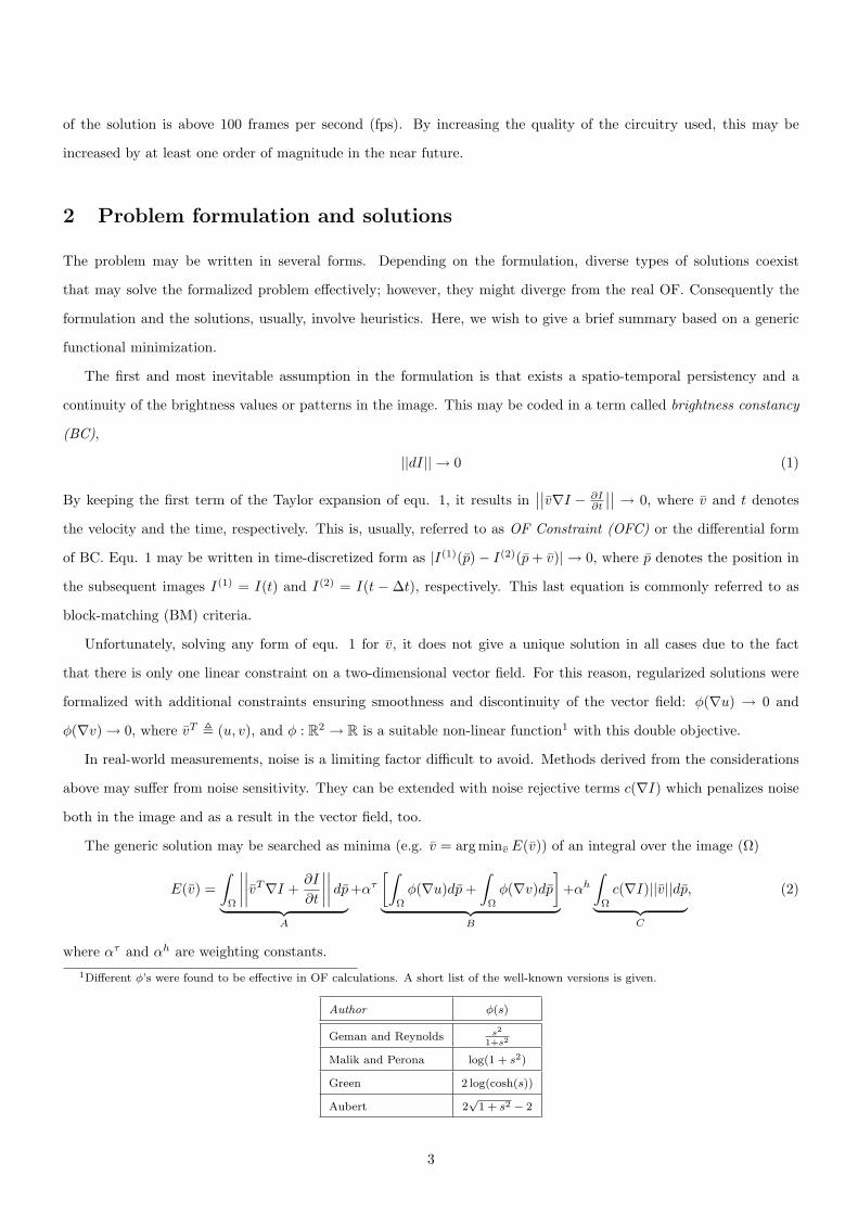
where ατ and αh are weighting constants.1Different φ’s were found to be effective in OF calculations. A short list of the well-known versions is given.

Author φ(s)

Geman and Reynolds s2

1+s2

Malik and Perona log(1 + s2)

Green 2 log(cosh(s))

Aubert 2√

1 + s2 − 2

3

In this functional, other functionals may be used as a plug-in replacement for terms meeting the objective of the

original term. Hence, term A may be replaced by the integral of BM instead of that of the OFC, or term B may be

extended with additional constraints too. In ref. [SJ96, GL96] authors found it important to prevent vector field from

rotation and divergence. (e.g.∫Ω

φ(div(v), rot(v))dp )

In its generic form, it is nearly impossible to have a fast and uniquely converging minimization of equ. 2; however,

most OF estimators, which we are currently aware of, can be fit in this equation.

Lucas and Kanade ([LK81]) provided the following form in early times of OF estimators

E(v) =∫

Ω

W ∗∣∣∣∣∣∣∣∣vT∇I +

∂I

∂t

∣∣∣∣∣∣∣∣ dp,

where a Gaussian convolution kernel W was used for providing smoothness of v, that has extended the regions in terms

of p where unique solutions exist. While the solution can be given directly by a matrix inversion (if non singular) the

solution of the Horn Schunk model (i.e. E(v) =∫Ω

∣∣∣∣vT∇I + ∂I∂t

∣∣∣∣22dp + ατ

∫Ω||∇u|| + ||∇v||dp) can be approached

iteratively, only [HS81].

A comprehensive analysis on the properties of functions left open in equ. 2, on the set of admissible solutions

(existance, unicity) along with a high quality solution is given in ref. [ADK99, AK02]. Unfortunately, there is still a very

hard trade-off between OF quality and processing time. The partial differential equations (PDE) dropping out from

the analysis of the equations above, usually, converge very slowly, hence they may not be applied in applications where

real-time processing is a criterion by means of limited power and in limited space. However, interesting simplifications

may be made, which opens space for invention in analog chip design. Many motion- and OF-chips were fabricated in

the past. Without going into details, they share many common properties such as:

• they are made for special purpose,

• they are, usually, called bio-inspired or neuromorphic due to their on-chip photo-sensors and cellular structure

(only local connections exist in a matrix structure) resemble to the retina or the primary visual cortex in most

engineers’ perspective,

• they operate in discrete space and continuous time,

• sometimes even the off-chip communication is made asynchronously via Address Event Representation (AER),

• VLSI elements are used either in mixed or mainly in analog (non saturated) mode,

• they either realize the corresponding Euler-Lagrange equation that are in loose relationship with considerations

above or are simple ad-hoc motion sensors (e.g. Elementary Motion Detector)

• the results are rather noisy.

In fact, the circuitry we relied on (CNN) shares many of these charateristics. It is called ”bio-inspired”, cellularly

structured, implemented in analog VLSI, operates in continiuous time, it is compact. But, in contrast to all of them,

4

it is proved to be general purpose (via Turing equivalence) leaving space for analogic programmability. At the first

look, CNN may be perceived as a well parameterizable PDE solver. The most straightforward approach would imply

solutions that realize some of these PDEs on CNN-UM. This can be done by decomposing the PDE based solution into

CNN friendly system of equations. The raising difficulties are, usually, two-fold. On the one hand, the non-linear terms

of the resulted PDEs, usually, require calculations of divisions and/or H.O.T. On the other hand, the convolutional

structure of the CNN (which involves the spatial invariant criteria) is, usually, broken by the PDEs resulted.

In our solution, we constructed a stochastic framework in which the maximum of the probability distribution

function (PDF) p(v|I(1), I(2)) was searched (i.e. v = arg maxv p(v|I(1), I(2))). This was done to let multiple-scale view

of the images cooporate in a non-deterministic way and lead to a Bayes optimal resolution of the trade-off between

spatial bandwidth and accuracy (see the next section).

Interestingly, the algorithm obtained by the considerations above uses very simple parallel operations that can be

executed on CNN-UM and exploits its fully parallel nature. The experiments show that it is extremely accurate on

simple tests (note the sub-pixel accuracy in fig. 6) and on standard tests it remains fair (even on aVLSI) compared

to complex digital implementations. Furthermore, it operates over 100 fps, which reserves a unique place for it.

3 Block or Region Matching Based Techniques

The major advantages of using BM is the ability to successfully suppress image flicker and its simplicity in hardware

realization.

Definition 1. Region or block is a collection of pixels that are located within the boundaries of size r around p.

Rqp = (x, y) : ||(x, y)− p||∞ < r , r = 2q,

where q refers to the size of the region in logarithmic scale. Without loss of generality we may use any type of

norm but for practical reasons the applied norm is l∞ or maximum norm.

Definition 2. The measure Summed Squared Difference of two images at p = (x, y) in a given region is,

SSD(I(1), I(2), Rqp) =

1|Rq

p|∑

ξ∈Rqp

||I(1)(ξ)− I(2)(ξ)||2.

Without loosing most of the important characteristics of the squared differences, we can also use the norm l1,

which is particularly important in CNN implementation. Note that |Rqp| is not a norm but the size of the set (i.e. the

area of the region) which is, obviously, constant for a fixed q.

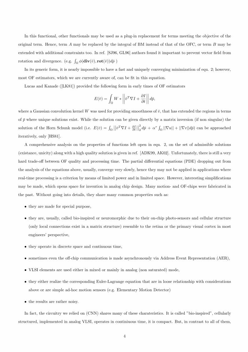
The simplest BM approach would mean a search for the best match or fit of a particular region in an image (I(1))

around a pixel (p) by offsetting the region by ∆p = v ·∆t in the image (I(2)). The measure is called Displaced Frame

Difference (DFD) (see fig. 1) and can be defined as

DFD(I(1), I(2),∆p, Rqp) =

1|Rq

p|∑

ξ∈Rqp

|I(1)(ξ + ∆p)− I(2)(ξ)|. (3)

5

I

I

∆2

1

Rp

p

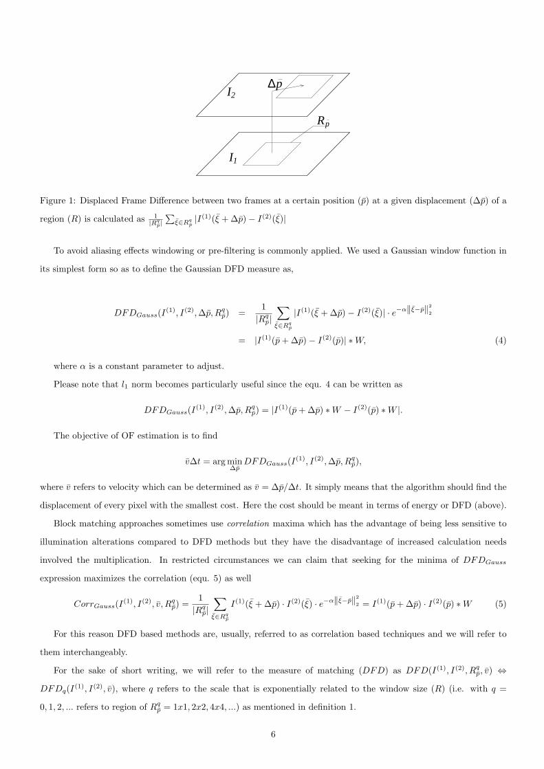
Figure 1: Displaced Frame Difference between two frames at a certain position (p) at a given displacement (∆p) of a

region (R) is calculated as 1|Rq

p|∑

ξ∈Rqp|I(1)(ξ + ∆p)− I(2)(ξ)|

To avoid aliasing effects windowing or pre-filtering is commonly applied. We used a Gaussian window function in

its simplest form so as to define the Gaussian DFD measure as,

DFDGauss(I(1), I(2),∆p, Rqp) =

1|Rq

p|∑

ξ∈Rqp

|I(1)(ξ + ∆p)− I(2)(ξ)| · e−α‖ξ−p‖22

= |I(1)(p + ∆p)− I(2)(p)| ∗W, (4)

where α is a constant parameter to adjust.

Please note that l1 norm becomes particularly useful since the equ. 4 can be written as

DFDGauss(I(1), I(2),∆p, Rqp) = |I(1)(p + ∆p) ∗W − I(2)(p) ∗W |.

The objective of OF estimation is to find

v∆t = arg min∆p

DFDGauss(I(1), I(2),∆p, Rqp),

where v refers to velocity which can be determined as v = ∆p/∆t. It simply means that the algorithm should find the

displacement of every pixel with the smallest cost. Here the cost should be meant in terms of energy or DFD (above).

Block matching approaches sometimes use correlation maxima which has the advantage of being less sensitive to

illumination alterations compared to DFD methods but they have the disadvantage of increased calculation needs

involved the multiplication. In restricted circumstances we can claim that seeking for the minima of DFDGauss

expression maximizes the correlation (equ. 5) as well

CorrGauss(I(1), I(2), v, Rqp) =

1|Rq

p|∑

ξ∈Rqp

I(1)(ξ + ∆p) · I(2)(ξ) · e−α‖ξ−p‖22 = I(1)(p + ∆p) · I(2)(p) ∗W (5)

For this reason DFD based methods are, usually, referred to as correlation based techniques and we will refer to

them interchangeably.

For the sake of short writing, we will refer to the measure of matching (DFD) as DFD(I(1), I(2), Rqp, v) ⇔

DFDq(I(1), I(2), v), where q refers to the scale that is exponentially related to the window size (R) (i.e. with q =

0, 1, 2, ... refers to region of Rqp = 1x1, 2x2, 4x4, ...) as mentioned in definition 1.

6

When larger Gaussian window (W in equ. 4) is applied, thanks to the averaging characteristics of the window,

will result in an image with degraded spatial bandwidth.

The blur caused by these integrating type of filters (such as window functions) is equivalent to applying a bandwidth

degrader or changing the view of an image to a larger scale (see appx. A). In the algorithm we propose, we combine

multi-scale (i.e. sections of the scale space ) information of a single image but we will not estimate the optimal scales

to use (see ref. [Wit83]).

4 Ambiguities in Optical Flow Techniques

The ambiguities that spoil the measurement of the OF may be explained in terms of block matching, too; There are

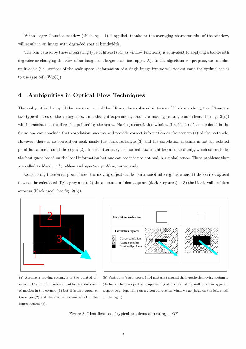
two typical cases of the ambiguities. In a thought experiment, assume a moving rectangle as indicated in fig. 2(a))

which translates in the direction pointed by the arrow. Having a correlation window (i.e. block) of size depicted in the

figure one can conclude that correlation maxima will provide correct information at the corners (1) of the rectangle.

However, there is no correlation peak inside the black rectangle (3) and the correlation maxima is not an isolated

point but a line around the edges (2). In the latter case, the normal flow might be calculated only, which seems to be

the best guess based on the local information but one can see it is not optimal in a global sense. These problems they

are called as blank wall problem and aperture problem, respectively.

Considering these error prone cases, the moving object can be partitioned into regions where 1) the correct optical

flow can be calculated (light grey area), 2) the aperture problem appears (dark grey area) or 3) the blank wall problem

appears (black area) (see fig. 2(b)).

13

2

(a) Assume a moving rectangle in the pointed di-

rection. Correlation maxima identifies the direction

of motion in the corners (1) but it is ambiguous at

the edges (2) and there is no maxima at all in the

center regions (3).

Aperture problem

Correct correlation

Blank wall problem

Correlation regions:

Correlation window size

(b) Partitions (slash, cross, filled patterns) around the hypothetic moving rectangle

(dashed) where no problem, aperture problem and blank wall problem appears,

respectively, depending on a given correlation window size (large on the left, small

on the right).

Figure 2: Identification of typical problems appearing in OF

7

To overcome these problems one might suggests to increase the correlation window size but it would lead

• to the gradual decrease of bandwidth and,

• to the quadratic increase in computational needs (and time).

This dilemma is called the bandwidth/accuracy trade-off.

In our model, the dilemma is hoped to be gradually removed. In the hierarchic calculation schema (explained later

in sec. 5) the CNN provides an alternative computational scheme that solves the Gaussian shaping and correlation

simultaneously in square root increase of time.

The similarity between this dilemma and equ. 2 should be noted. Equ. 2 is written in a form to overcome the

OFC ambiguities by means of the neighborhood while keeping the OFC term minimal.

5 Bayesian Incorporation of Scales

According to the considerations of the previous section, one can see that the main source of distortions in the search

for DFD minima (or correlation maxima) is rooted in the applied measurement technique. One has to note that using

the differential form of the OFC does not help. The problem appears similarly, as a singularity of the corresponding

matrices. To overcome these problems, we propose a stochastic model by associating a measure of fitness (DFD) with

a similarity likelihood as,

pq(I(2)|v, I(1)) ∝ exp−DFDq(I(1), I(2), v)

. (6)

There are several notes we have to make here:

• The form of the fitness (DFD) is somewhat arbitrary which could be appropriate in many other forms.

• The only property we expect from the likelihood is to be inversely proportional to this particular fitness.

• This likelihood defines a measure proportional to the likeliness of being the correct warp of a region of size 2qx2q

from one image to the other. (e.g. the normalization would be over the I(2)).

Based on this likelihood, by Bayes theorem for the aposterior we have,

pq(v|I(1), I(2)) =pq(I(2)|v, I(1)) pq(v|I(1))

pq(I(2)|I(1))∝ pq(I(2)|v, I(1)) pq(v|I(1))

Since the denominator does not depend on v for which we are to maximize this expression, we can drop it. As it is

common in Bayesian decisions, having a good prior hypothesis is crucial in making reasonable decisions. This is the

Ockham’s razor. In OF calculus, the question of good priors had left space for a lot of debates in the literature too

(ref. [AB86]).

Thinking in multiple scales, from the study of ambiguous situations, we might conclude that the prior can be the

larger scale (q + 1) estimation of the OF. This helps to reconstruct the OF at a given (q) scale with propagating the

8

information available at the larger scale. (i.e. associate pq(v|I(1))← pq+1(v|I(1), I(2))) as,

pq(v|I(1), I(2)) ∝ pq(I(2)|v, I(1)) pq+1(v|I(1), I(2)).

This recursive scheme can be written in explicit form as,

p(v|I(1), I(2)) ∝ p0(v)∏q

pq(I(2)|v, I(1)) = p0(v) exp

[−∑

q

DFDq(I(1), I(2), v)

].

Certainly, we are interested in the vector field (or OF) at the finest scale which is,

v = arg maxv

p(v|I(1), I(2)) = arg minv

[− log p0(v) +

∑q

DFDq(I(1), I(2), v)

]. (7)

Note that, however, we formulated the problem is in the log-domain, by disregarding the constant first term in

equ. 7, the calculation to be done here remains as simple as addition of DFDs and an extremum search.

An alternative formulation was suggested by Cs. Szepesvari in a personal communication leading essentially to the

same results (For details see appx. D).

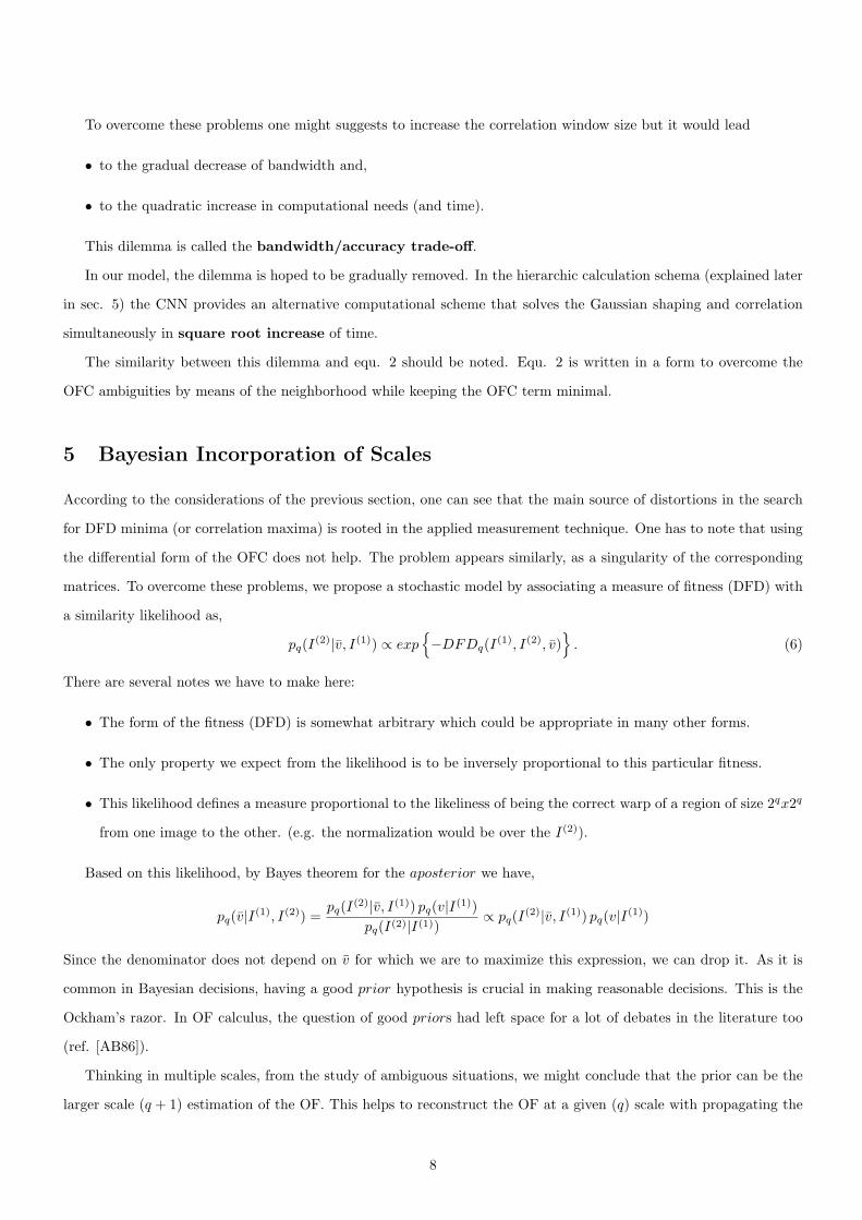
The resulted calculation scheme defines a Bayesian incorporation of the multi-scale measurements. (see fig. 3)

Incorporation at scale q

Hypothesis at scale q

Best guess at scale q

Measurement at scale q+1

Measurement at scale q

Best guess at scale q+1

Null hypothesis

Figure 3: Bayesian incorporation of multiple scales: optimal PDF (probablity distribution function) at scale q + 1

becomes a hypothesis at scale q. This, along with the likelihood (measurement) at scale q, can give the posterior (best

guess) at scale q by Bayesian inference.

This figure explains how PDFs are propagated through scales.

Assume a null hypothesis (e.g. pq(v) = const ), measure the fittness at every position with every possible motion

vector and associate it with the corresponding probability function (equ. 6). During this measure, a window function

(W in equ. 5) was used, which corresponds to the scale (q). Multiply these PDFs then assume it to be the hypothesis

at next step. In the next step, use a smaller window for the measurement. And repeat, until the predefined window

size is reached.

In this induction-like rule, we will need a prior for the whole model. We choose a zero mean Gaussian for this

which biases for slow speed. Preference of such has been found to play role in human perception [WA98]. In most cases

9

it is not necessary to have a well parametrized null hypothesis (covariance), since it affects the results only marginally

which is, in fact, quite a desirable characteristic of a model. Note that, if Gaussian was chosen as a prior, then the

calculation of the expression log p(v0) becomes simply quadratic.

This model should optimally resolve the trade-off in sec. 4, where the term optimal is meant in Bayesian sense.

The recursive calculation scheme above might recall ref. [WC99], in which the author got similar conclusion to ours

with respect to calculating the Bayesian optimal distribution. Noteworthly, he has found that subsequent experiments

(or measurements), even with a simplistic model of the ”world” (prior), can gradually reinforce or refute hypotheses

and, finally, they are incorporated in an optimal estimation.

It has to be noted that numerous multi-scale (ref.[BB95, Ana89, BAK91, Enc86, Gla87, MP98]) and also Bayesian

OF models (e.g. ref. [Zel04], [LM95]), are known in the literature. Furthermore, in ref. [Sim99] a Bayesian multi-scale

differential OF estimation by Simoncelli2 was published.

6 The Algorithm

6.1 The First Approach

First, let us overview the steps of the proposed algorithm.

• initiate the DFD with null hypothesis,

• measure DFD at a scale,

• accumulate the DFD in order to obtain the log of optimal PDF at the current scale,

• repeat the last two steps for all scales,

• finally, select a minima of the accumulated DFD.

Writing it in pseudo code see alg. 1.

Algorithm 1.

log PDF generation

Initial DFD is either even or zero mean Gaussian

Cycle for scale (q)

2At surface level, it may seem that our model is similar to the one by Simoncelli, who also considered a probabilistic multi-scale

setup. However, Simoncelli’s assumption are rather different from ours. In particular, he worked with OFC-based models where he made

assumption on the distribution of the noise corrupting the images’ time derivative and the flow field, whilst we do not introduce flow-field

noise. He introduced multi-scale framework in which the mean and the covariance of the estimation is propagated (updated and corrected)

by a linear Kalman filter from higher scales to lower scales.

10

Cycle for position (p)

Cycle for displacement (v)

Cycle for DFD (ξ)

Accumulate for

DFD(v(p)) = 1|Rq

p|∑

ξ∈Rqp|I(1)(v + ξ)− I(2)(ξ)| ·W (ξ − p)

End cycle DFD

End cycle (v)

End cycle (p)

End Cycle (q)

MAP selection

Cycle for position (p)

Cycle for displacement (v)

copy vMAP (p) = arg maxv p(v(p))

End cycle (v)

End cycle (p)

Due to the extreme size of calculations (O(N7)), for having results in reasonable time, optimization is desirable.

We have found that by means of CNN-UM the reduction of the need of operations is somewhere in the magnitude of

O(N3) (see appx. B).

6.2 The Exploitation of the CNN Concept

To make the handling of the CNN core easier, one can decompose it into two parts. The first part is the autonomous

part (x = −x + A ∗ y), the second is a fix term part (B ∗ u + z) that contributes to the evolution of the equation as a

constant.

If, e.g., A = 0, called control mode, CNN simply copies the fix term into vector(image) x. Note the usefulness of

such a simple operation. It achieves a convolution and vector addition of an image of N2 pixels in a single step.

In the calculation of DFD (see right hand side (RHS) of equ. 3) one can notice a term which is an average of

differences of a particular region (Rqp) around the point p. This difference (i.e. I(1)− I(2)) can be calculated in control

mode by a [B0,0 = −1] 3 template. Naturally, a translation operator was applied to generate the shift of images before

the subsequent subtraction took place which can be achieved by a single B template operation. By putting an image

in u, applying [B0,1 = 1] results in a translated image copied into x.

3In general, template elements (i.e. Aij and Bij), if not indicated otherwise, are assumed to be zero.

11

The autonomous part of the CNN core can effectively calculate the average ( 1|R|∑

ξ∈R) of a given region as quick as,

for example, a pixel-wise difference calculation by means of an isotropic diffusion operator (i.e. A is central symmetric

positive definite with B = 0) This equation asymptotically approaches the average (i.e. x(t) → [x(0)]average) if

conservative BC is applied.

If we apply a masking window of Rqp that enables CNN to operate around a pixel p, then a diffusion operator

is able to calculate the average in this window. This recognition lets us spare the Cycle for DFD and save O(N2)

operations as shown below,

Algorithm 2.

log PDF generation

Cycle for scale (q)

Cycle for position (p)

Cycle for displacement (v)

Generate mask (Rqp) for the next CNN operations

Template running: Diff(v) = Translate(I(1), v)− I(2)

Template running: average of Diff within Rqp by means of a mask.

End cycle (v)

End cycle (p)

End Cycle (q)

Instead of calculating the simple DFD, the Gaussian windowed version (DFDGauss) can be obtained by dropping

the masking window and applying a single diffusion with impulse response exactly the same as the Gaussian windowing

function. (see appx. A). This step spares 2 cycles for p and adds a diffusion with few µsec expense. The gain on the

complexity of the algorithms is estimated in appx. B. See the modified algorithm below,

Algorithm 3.

log PDF generation

Cycle for scale (q)

Cycle for displacement (v)

Template running: Diff(v) = |Translate(I(1), v)− I(2)|.

Template running: Diffusion of Diff(v) for τq

End cycle (v)

12

End Cycle (q)

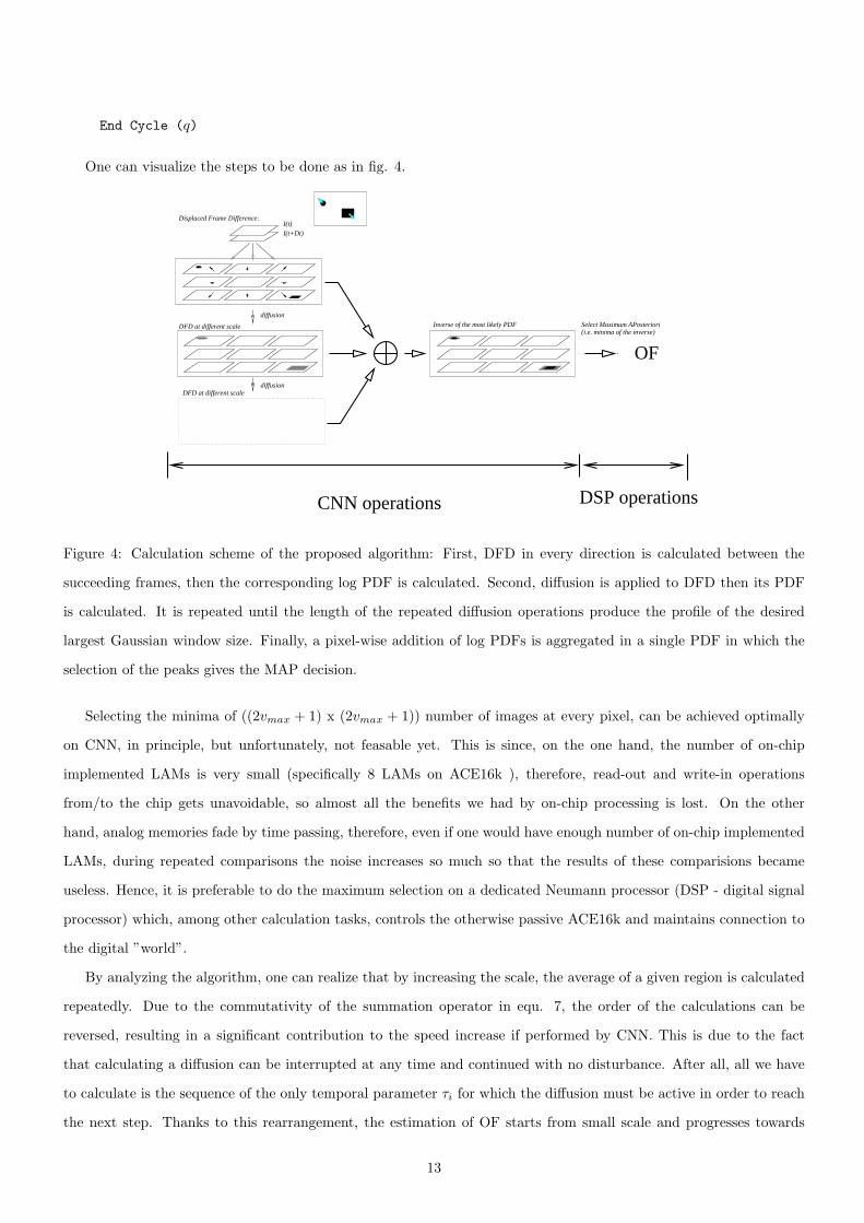
One can visualize the steps to be done as in fig. 4.

DFD at different scale Inverse of the most likely PDF Select Maximum APosteriori(i.e. minima of the inverse)

DFD at different scale

diffusion

diffusion

Displaced Frame Difference:

I(t+Dt)

I(t)

OF

DSP operationsCNN operations

Figure 4: Calculation scheme of the proposed algorithm: First, DFD in every direction is calculated between the

succeeding frames, then the corresponding log PDF is calculated. Second, diffusion is applied to DFD then its PDF

is calculated. It is repeated until the length of the repeated diffusion operations produce the profile of the desired

largest Gaussian window size. Finally, a pixel-wise addition of log PDFs is aggregated in a single PDF in which the

selection of the peaks gives the MAP decision.

Selecting the minima of ((2vmax + 1) x (2vmax + 1)) number of images at every pixel, can be achieved optimally

on CNN, in principle, but unfortunately, not feasable yet. This is since, on the one hand, the number of on-chip

implemented LAMs is very small (specifically 8 LAMs on ACE16k ), therefore, read-out and write-in operations

from/to the chip gets unavoidable, so almost all the benefits we had by on-chip processing is lost. On the other

hand, analog memories fade by time passing, therefore, even if one would have enough number of on-chip implemented

LAMs, during repeated comparisons the noise increases so much so that the results of these comparisions became

useless. Hence, it is preferable to do the maximum selection on a dedicated Neumann processor (DSP - digital signal

processor) which, among other calculation tasks, controls the otherwise passive ACE16k and maintains connection to

the digital ”world”.

By analyzing the algorithm, one can realize that by increasing the scale, the average of a given region is calculated

repeatedly. Due to the commutativity of the summation operator in equ. 7, the order of the calculations can be

reversed, resulting in a significant contribution to the speed increase if performed by CNN. This is due to the fact

that calculating a diffusion can be interrupted at any time and continued with no disturbance. After all, all we have

to calculate is the sequence of the only temporal parameter τi for which the diffusion must be active in order to reach

the next step. Thanks to this rearrangement, the estimation of OF starts from small scale and progresses towards

13

larger scales, while the PDFs multiply in between.

In appx. C, we publish on-chip diffusion tests achieved for standard test functions such as the Heaviside step

function and the rectangular test function. These tests make possible to estimate the chip’s diffusion time constant by

experience and give some heuristic analysis of the deterministic and stochastic noise sources distorting the measurement

of the DFDGauss.

7 Performance Analysis

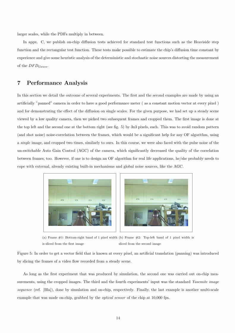
In this section we detail the outcome of several experiments. The first and the second examples are made by using an

artificially ”panned” camera in order to have a good performance meter ( as a constant motion vector at every pixel )

and for demonstrating the effect of the diffusion on single scales. For the given purpose, we had set up a steady scene

viewed by a low quality camera, then we picked two subsequent frames and cropped them. The first image is done at

the top left and the second one at the bottom right (see fig. 5) by 3x3 pixels, each. This was to avoid random pattern

(and shot noise) noise-correlation between the frames, which would be a significant help for any OF algorithm, using

a single image, and cropped two times, similarly to ours. In this course, we were also faced with the pulse noise of the

un-switchable Auto Gain Control (AGC) of the camera, which significantly decreased the quality of the correlation

between frames, too. However, if one is to design an OF algorithm for real life applications, he/she probably needs to

cope with external, already existing built-in mechanisms and global noise sources, like the AGC.

(a) Frame #1: Bottom-right band of 1 pixel width

is sliced from the first image

(b) Frame #2: Top-left band of 1 pixel width is

sliced from the second image

Figure 5: In order to get a vector field that is known at every pixel, an artificial translation (panning) was introduced

by slicing the frames of a video flow recorded from a steady scene.

As long as the first experiment that was produced by simulation, the second one was carried out on-chip mea-

surements, using the cropped images. The third and the fourth experiments’ input was the standard Yosemite image

sequence (ref. [Bla]), done by simulation and on-chip, respectively. Finally, the last example is another multi-scale

example that was made on-chip, grabbed by the optical sensor of the chip at 10,000 fps.

14

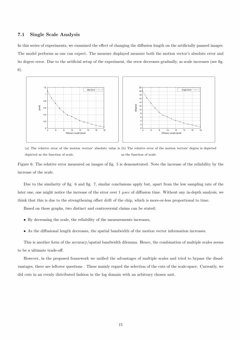
7.1 Single Scale Analysis

In this series of experiments, we examined the effect of changing the diffusion length on the artificially panned images.

The model performs as one can expect. The measure displayed measure both the motion vector’s absolute error and

its degree error. Due to the artificial setup of the experiment, the error decreases gradually, as scale increases (see fig.

6).

0

0.2

0.4

0.6

0.8

1

1.2

4 6 8 10 12 14 16 18

[pix

el]

Diffusion Length [pixel]

Abs Error

(a) The relative error of the motion vectors’ absolute value is

depicted as the function of scale.

0

2

4

6

8

10

12

14

16

18

20

22

4 6 8 10 12 14 16 18

[Deg

ree]

Diffusion Length [pixel]

Angle Error

(b) The relative error of the motion vectors’ degree is depicted

as the function of scale.

Figure 6: The relative error measured on images of fig. 5 is demonstrated. Note the increase of the reliability by the

increase of the scale.

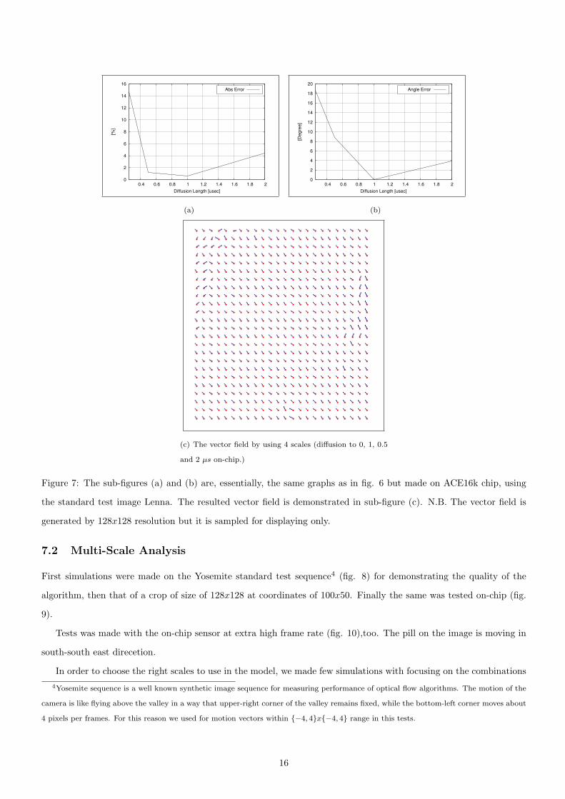
Due to the similarity of fig. 6 and fig. 7, similar conclusions apply but, apart from the low sampling rate of the

later one, one might notice the increase of the error over 1 µsec of diffusion time. Without any in-depth analysis, we

think that this is due to the strengthening offset drift of the chip, which is more-or-less proportional to time.

Based on these graphs, two distinct and controversial claims can be stated:

• By decreasing the scale, the reliability of the measurements increases,

• As the diffusional length decreases, the spatial bandwidth of the motion vector information increases.

This is another form of the accuracy/spatial bandwidth dilemma. Hence, the combination of multiple scales seems

to be a ultimate trade-off.

However, in the proposed framework we unified the advantages of multiple scales and tried to bypass the disad-

vantages, there are leftover questions . These mainly regard the selection of the cuts of the scale-space. Currently, we

did cuts in an evenly distributed fashion in the log domain with an arbitrary chosen unit.

15

0

2

4

6

8

10

12

14

16

0.4 0.6 0.8 1 1.2 1.4 1.6 1.8 2

[%]

Diffusion Length [usec]

Abs Error

(a)

0

2

4

6

8

10

12

14

16

18

20

0.4 0.6 0.8 1 1.2 1.4 1.6 1.8 2

[Deg

ree]

Diffusion Length [usec]

Angle Error

(b)

(c) The vector field by using 4 scales (diffusion to 0, 1, 0.5

and 2 µs on-chip.)

Figure 7: The sub-figures (a) and (b) are, essentially, the same graphs as in fig. 6 but made on ACE16k chip, using

the standard test image Lenna. The resulted vector field is demonstrated in sub-figure (c). N.B. The vector field is

generated by 128x128 resolution but it is sampled for displaying only.

7.2 Multi-Scale Analysis

First simulations were made on the Yosemite standard test sequence4 (fig. 8) for demonstrating the quality of the

algorithm, then that of a crop of size of 128x128 at coordinates of 100x50. Finally the same was tested on-chip (fig.

9).

Tests was made with the on-chip sensor at extra high frame rate (fig. 10),too. The pill on the image is moving in

south-south east direcetion.

In order to choose the right scales to use in the model, we made few simulations with focusing on the combinations4Yosemite sequence is a well known synthetic image sequence for measuring performance of optical flow algorithms. The motion of the

camera is like flying above the valley in a way that upper-right corner of the valley remains fixed, while the bottom-left corner moves about

4 pixels per frames. For this reason we used for motion vectors within −4, 4x−4, 4 range in this tests.

16

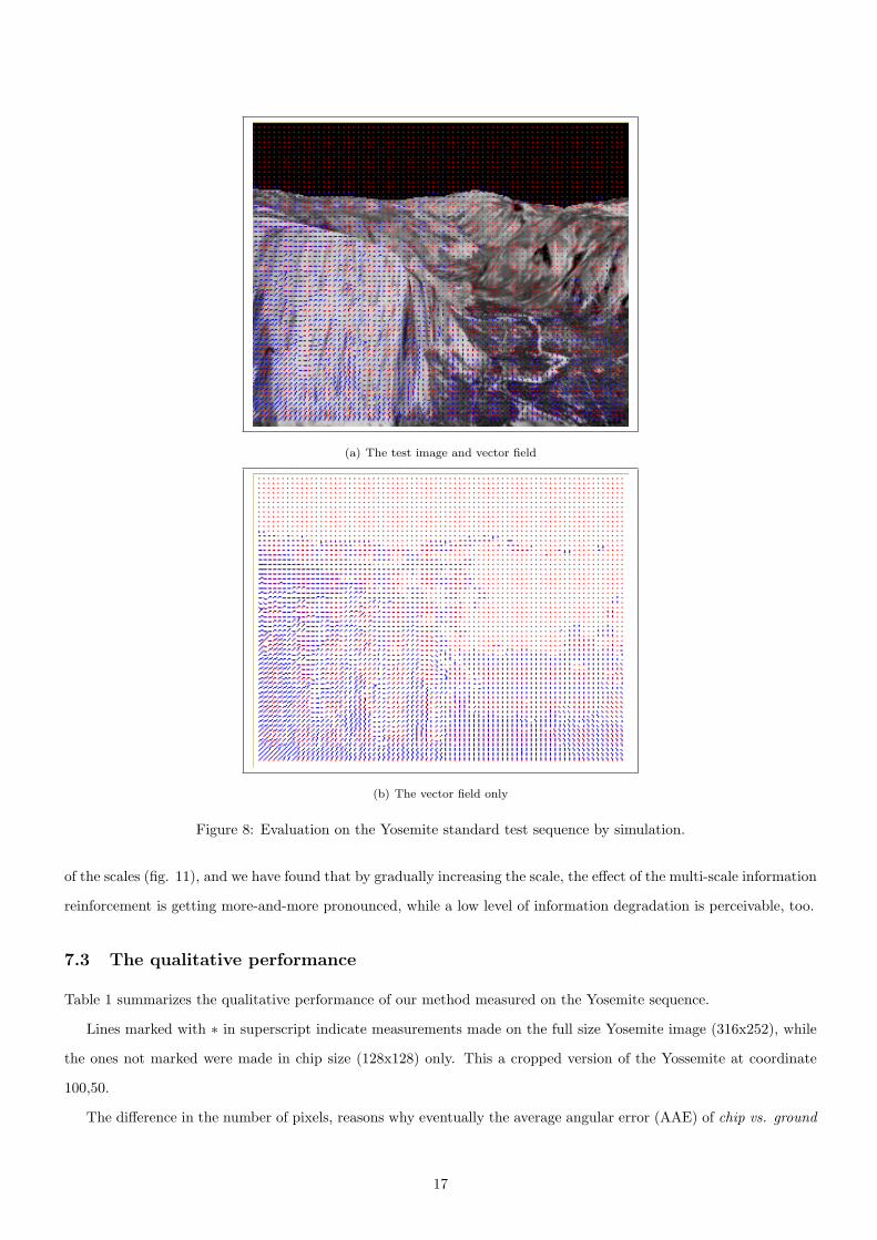
(a) The test image and vector field

(b) The vector field only

Figure 8: Evaluation on the Yosemite standard test sequence by simulation.

of the scales (fig. 11), and we have found that by gradually increasing the scale, the effect of the multi-scale information

reinforcement is getting more-and-more pronounced, while a low level of information degradation is perceivable, too.

7.3 The qualitative performance

Table 1 summarizes the qualitative performance of our method measured on the Yosemite sequence.

Lines marked with ∗ in superscript indicate measurements made on the full size Yosemite image (316x252), while

the ones not marked were made in chip size (128x128) only. This a cropped version of the Yossemite at coordinate

100,50.

The difference in the number of pixels, reasons why eventually the average angular error (AAE) of chip vs. ground

17

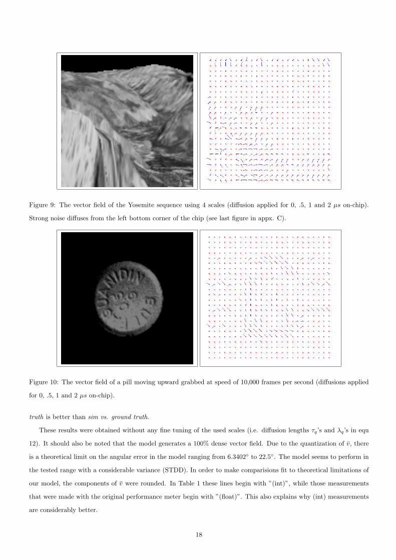
Figure 9: The vector field of the Yosemite sequence using 4 scales (diffusion applied for 0, .5, 1 and 2 µs on-chip).

Strong noise diffuses from the left bottom corner of the chip (see last figure in appx. C).

Figure 10: The vector field of a pill moving upward grabbed at speed of 10,000 frames per second (diffusions applied

for 0, .5, 1 and 2 µs on-chip).

truth is better than sim vs. ground truth.

These results were obtained without any fine tuning of the used scales (i.e. diffusion lengths τq’s and λq’s in equ

12). It should also be noted that the model generates a 100% dense vector field. Due to the quantization of v, there

is a theoretical limit on the angular error in the model ranging from 6.3402 to 22.5. The model seems to perform in

the tested range with a considerable variance (STDD). In order to make comparisions fit to theoretical limitations of

our model, the components of v were rounded. In Table 1 these lines begin with ”(int)”, while those measurements

that were made with the original performance meter begin with ”(float)”. This also explains why (int) measurements

are considerably better.

18

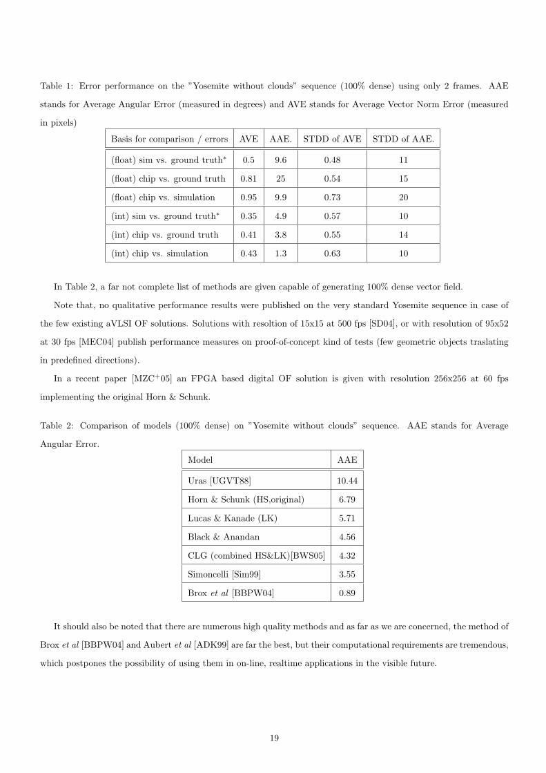
Table 1: Error performance on the ”Yosemite without clouds” sequence (100% dense) using only 2 frames. AAE

stands for Average Angular Error (measured in degrees) and AVE stands for Average Vector Norm Error (measured

in pixels)

Basis for comparison / errors AVE AAE. STDD of AVE STDD of AAE.

(float) sim vs. ground truth∗ 0.5 9.6 0.48 11

(float) chip vs. ground truth 0.81 25 0.54 15

(float) chip vs. simulation 0.95 9.9 0.73 20

(int) sim vs. ground truth∗ 0.35 4.9 0.57 10

(int) chip vs. ground truth 0.41 3.8 0.55 14

(int) chip vs. simulation 0.43 1.3 0.63 10

In Table 2, a far not complete list of methods are given capable of generating 100% dense vector field.

Note that, no qualitative performance results were published on the very standard Yosemite sequence in case of

the few existing aVLSI OF solutions. Solutions with resoltion of 15x15 at 500 fps [SD04], or with resolution of 95x52

at 30 fps [MEC04] publish performance measures on proof-of-concept kind of tests (few geometric objects traslating

in predefined directions).

In a recent paper [MZC+05] an FPGA based digital OF solution is given with resolution 256x256 at 60 fps

implementing the original Horn & Schunk.

Table 2: Comparison of models (100% dense) on ”Yosemite without clouds” sequence. AAE stands for Average

Angular Error.

Model AAE

Uras [UGVT88] 10.44

Horn & Schunk (HS,original) 6.79

Lucas & Kanade (LK) 5.71

Black & Anandan 4.56

CLG (combined HS&LK)[BWS05] 4.32

Simoncelli [Sim99] 3.55

Brox et al [BBPW04] 0.89

It should also be noted that there are numerous high quality methods and as far as we are concerned, the method of

Brox et al [BBPW04] and Aubert et al [ADK99] are far the best, but their computational requirements are tremendous,

which postpones the possibility of using them in on-line, realtime applications in the visible future.

19

8 Conclusion

Based on some of the known phenomena attributed to VSS (Bayesian inference, multi-scale view), we have formulated

a simple, but usable multi-scale OF algorithm that was shown to be applicable in a mixed signal VLSI technique.

As other experiments showed, simple ad-hoc approaches (such as edge detection with center-surround filters) can

easily improve the performance of the developed algorithm but here we have concentrated on the formalism itself

which proves to be powerful both in computational complexity and in accuracy on a general purpose aVLSI hardware

versus special purpose hardware with the largest resolution. The resolution of the chip we used was enough to

measure reasonable performance meter on standard image sequence (Yosemite) over 100 fps. Formerly, the conducted

simulations pointed out a theoretical limit on the accuracy of the algorithm, which the analog on-chip results seem to

get close to, robustly. This is achieved as fast as none of the existing solutions exceeding our accuracy, even in digital

hardware at this resolution.

Although the main disadvantage of the algorithm is the inevitably large memory needs, which increases quadrati-

cally with the size of the motion vector but, as we have shown, it can be kept limited.

Further investigation should be made to determine the optimal distribution of scales on given images (scale space

analysis) what is currently made as a regular sampling only. It is also desirable to determine if the aggregated PDF

provides more information than a single vector field. We assume that this increased information may be exploited

easily in standard image processing tasks such as segmentation.

References

[AB86] E.H. Adelson and J.R. Bergen. The extraction of spatio temporal energy in machine and human vision.

In Proc. IEEE Workshop on Visual Motion, pages 151–166, 1986.

[ADK99] G. Aubert, R. Deriche, and P. Knorprobst. Computing of via variational techniques. SIAM, J. of Appl.

Math (JAM), 60(1):156–182, 1999.

[AK02] G. Aubert and P. Knorprobst. Mathematcial Problems in Image Processing,Partial Differential Equations

and Calculus of Variations. Springer-Verlag, New York, 2002.

[Ana89] P. Anandan. A computational framework and an algorithm for the measurement of visual motion. Intl.

Jour. of Computer Vision (IJCV), 2:283–310, 1989.

[BAK91] R. Battiti, E. Amaldi, and C. Koch. Computing optical flow across multiple scales: An adaptive coarse-

to-fine strategy. Intl. Jour. of Computer Vision (IJCV), 2(6):133–145, 1991.

[BB95] S. S. Beauchemin and J. L. Barron. The computation of optical flow. ACM Computing Surveys, 27(3):433–

467, 1995.

20

[BBPW04] T. Brox, A. Bruhn, N. Papenberg, and J. Weickert. High accuracy optical flow estimation based on a

theory for warping. In J. Matas T. Pajdla, editor, Computer Vision - ECCV 2004, Lecture Notes in

Computer Science, volume 3024, pages 25–36, Berlin, 2004. Springer.

[BJ96] M. J. Black and A. D. Jepson. Eigentracking: Robust matching and tracking of articulated objects using

a view-based representation. Technical Report RBVC-TR-96-50, Technical Report at Univ. of Toronto,

Dept. of Comp. Sci, Oct 1996.

[Bla] Michael J. Black. Yosemite image sequences. http://www.cs.brown.edu/people/black/Sequences/yosemite.tar.gz.

[BWS05] Andres Bruhn, Joachim Weickert, and Christoph Schnorr. Lucas/kanade meets horn/schunck: Combining

local and global optic flow methods. Intl. Jour. of Computer Vision (IJCV), 61(3):211–231, 2005.

[ECdSM97] R. Etienne-Cummings, J. Van der Spiegel, and P. Muller. A focal plane visual motion measurement

sensor. IEEE Trans. on Circuits and Systems I (TCAS), 44(1):55–56, Jan 1997.

[Enc86] W. Enckelmann. Investigation of multigrid algorithms for the estimation of optical flow fields in images

sequences. In Proc of. IEEE Workshop on Motion: Representation and Analysis, pages 81–87, Charleston,

South Carolina, May 1986.

[GL96] F. Guichard and L.Rudin. Accurate estimation of discontinuous optical flow by minimizing divergence

related functionals. In Proc. Int’l Conf. on Image Proc. (ICIP96), volume 1, pages 497–500, Lausanne

Switzerland, Sept 1996.

[Gla87] F. C. Glazer. Computation of optical flow by multilevel relaxation. Technical Report COINS-TR-87-64,

Univ. of Massachusetts, 1987.

[Hee88] D. J. Heeger. Optical flow using spatio-temporal filters. Intl. Jour. of Computer Vision (IJCV), 1:279–302,

1988.

[HKLM88] J. Hutchinson, C. Koch, J. Luo, and C. Mead. Computing motion using analog and binary resistive

networks. IEEE Computer, 21(3):52–64, March 1988.

[HKSL90] J. Harris, C. Koch, E. Staats, and J. Luo. Analog hardware for detecting discontinuities in early vision.

Intl. Jour. of Computer Vision (IJCV), 4:211–223, 1990.

[HS81] B.K.P. Horn and G. Schunk. Determining optical flow. Artificial Intelligence (AI), 17:185–203, 1981.

[HS02] C. M. Higgins and S. A. Shams. A bilogocially inspired modular vlsi system for visual measurement of

self-motion. IEEE Trans. on Sensors and Systems (SS), 2(6):508–528, Dec 2002.

[KM96] C. Koch and B. Mathur. Neuromorphic vision chips. IEEE Spectrum, 33(5):38–46, May 1996.

21

[KSK97] J. Kramer, R. Sarpeshkar, and C. Koch. Pulse-based analog vlsi velocity sensors. IEEE Trans. on Circuits

and Systems II (TCAS), 44:86–101, Feb 1997.

[Liu98] S. C. Liu. Silicon retina with adaptive filtering properties. In S. A. Solla M. I. Jordan, M.J. Kearns,

editor, Advances in Neural Information Processing Systems (ANIPS), volume 10, pages 712–718. MIT

Press, 1998.

[LK81] B. D. Lucas and T. Kanade. An iterative image registration technique with an application to stereo vision.

In Proc. of image understanding workshop, pages 121–130, 1981.

[LM95] R. Laganiere and A. Mitiche. Direct bayesian interpretation of visual motion. Robotics and Autonomous

Systems (RAS), 14(4):247–254, June 1995.

[MEC04] S. Mehta and R. Etienne-Cummings. Normal optical flow measurement on a cmos aps images. In IEEE

Int. Simp. on Circ. And Sys. (ISCAS’04), pages 23–26, Vancouver, Canada, May 2004.

[MP98] Etienne Memin and Patrick Perez. Dense estimation and object based segmentation of the optical flow

with robust techniques. IEEE Trans. on Image Processing (IP), 7(5), May 1998.

[MZC+05] Jose’ L. Martl’n, Aitzol Zuloaga, Carlos Cuadrado, Jesu’s La’ zaro, and Unai Bidarte. Hardware im-

plementation of optical flow constraint equation using fpgas. Comp. Vision and Image Understanding

(CVIU), 98:462–490, 2005.

[RF04] F. Ruffier and N. Franceschini. Visual guided micro-aerial vehicle: automatic take off, terrain following,

landing and wind reaction. In Proc. of Int’l Conf. on Robotics & Autom (ICRA2004), New Orleans, April

2004.

[SD04] A. Stocker and R. Douglas. Analog integrated 2-d optical flow sensor with programmable pixels. In IEEE

Int. Simp. on Circ. And Sys. (ISCAS’04), volume 3, pages 9–12, Vancouver, Canada, May 2004.

[Sim99] Eero P. Simoncelli. Bayesian Multi-Scale Differential Optical Flow, volume 2, chapter 14, pages 397–422.

Academic Press, April 1999.

[SJ96] S.N.Gupta and J.L.Prince. On div-curl regularization for motion estimation in 3-d volumetric imaging. In

Proc. Int’l Conf. on Image Proc. (ICIP96), volume 1, pages 929–932, Lausanne Switzerland, Sept 1996.

[SL01] B. Szatmary and A. Lorincz. Indepent component analysis of temporal sequences subject to constraints

by lgn inputs yields all the three major cell types of the primary visual cortex. Jour. of Computational

Neurosci. (JCN), 11:241–248, 2001.

[SRC98] B. Shi, T. Roska, and L. O. Chua. Estimating optical flow with cellular neural networks. International

Journal of Circuits Theory and Applications (CTA), 26:343–364, 1998.

22

[UGVT88] S. Uras, F. Girosi, A. Verri, and V. Torre. A computational approach to motion perception. Biological

Cibernetics (BC), 60:79–87, 1988.

[WA98] Y. Weiss and E.H. Adelson. Slow and smooth: Bayesian theory of combination of local motion signals in

human vision. Technical Report Tech. Rep 1624, AI Lab. Massachusetts Institute of Technology, Boston,

Cambridge, MA, 1998.

[WC99] Ranxiao Frances Wang and James E. Cutting. A probabilistic model for recovering camera translation.

Comp. Vision and Image Understanding (CVIU), 76(3):205–212, Dec 1999.

[Wit83] A. P. Witkin. Scale space filtering. In Proc. of Int. Joint Conference on Artificial Intelligence (IJCAI),

Karlsruhe Germany, 1983.

[Zel04] J. S. Zelek. Bayesian real-time optical flow. Elsevier Vision & Image Computing Journal (VICJ), 22:1051–

1069, 2004.

A The diffusion PDE and the corresponding IIR equivalence

A.1 Diffusion PDE

Next we brief the solution of a diffusion PDE, and compare it to the use of a Gaussian window function, and ,finally,

point out their equivalence.

The following differential equation describes a diffusion process

D

2∇f(x, t)− ∂f(x, t)

∂t= 0.

Let the solution be fj(x, t), where j refers to the initial conditions. First, set it to

f1(x, t = 0) = δx,0,

then solution is

f1(x, t) =1√2πt

exp−x2

2t

. (8)

Now, having a vector composed of samples s(i) in discrete space as an initial condition as,

f2(x, t = 0) =∑

i

s(i) δx,i,

then the solution is,

f2(x, t) =∑

i

s(i)f1(x + i, t) = s ∗ f1(x, t), (9)

where ’∗’ denotes the convolution operator, and i iterates through the discrete space.

23

A.2 Gaussian convolution window

Infinite Impulse Response (IIR) filtering means

y = s ∗ IIR (10)

where y is the filter output, IIR is the filter and s is the input. If IIR is assigned to a certain Gaussian function (e.g.

equ. 8), then equ. 10 turns to be equivalent to equ. 9 with a proper time step (i.e. t = t0), which means, applying

diffusion and using convolution of Gaussian filter provides the the same result.

From equ. 10, one can also conclude that if diffusion is done as an elementary operator, then Gaussian window

filtering is accelerated the by O(N2) orders of magnitude.

B Algorithm Complexity

The complexity of algorithms is given in this section.

First, the alg. 1 is analyzed.

• It has to calculate the DFD at every pixel O(N2), for all possible vectors O(M2),

• then, the convolution for kernel size K at every scale (S), for O(N2,M2,K2, S) cost.

• Finally, get the maxima on a per pixel basis for O(N2,M2) const.

Hence, the upper limit is O(N2,M2,K2, S).

Second, the complexity of alg. 3 is given.

• The DFD is done in O(M2) time.

• The generation diffused versions for O(M2,K)

• Finally, get the maxima at every pixel on DSP O(N2,M2)

Note that, this solution has is only O(N2,M2) complexity since all the rests is done in CNN, in the device that is

essentially parallel and the speed of which does not depend on the number of pixels.

Probably, it is not fair to compare a sequential (Neumann) architecture to a fully parallel analog one (CNN) in

terms of complexity. For this reason, we might refer to the complexity term as a complexity in CNN sense opposed

to the traditional complexity concept; complexity in Neumann sense.

C On-chip Diffusion

Unfortunately, analog circuits always face noise problems, hence implemented algorithms need tuned to be robust

against it. For this reason, we have recorded in-diffusion fix-pattern noise transfer characteristics of the Heaviside

step-function (fig. 13) and the rectangular function on the ACE16k (fig. 15).

24

Fix-pattern noise was measured by loading a zero level picture input into a LAM, then after a few micro-seconds

of diffusion, it was read-back from the same LAM.

We registered the following type of errors

• There was a bias towards white (in CNN terms it is referred to as -1 and associated with the negative supply

voltage) in the middle region of the chip that is probably due to the supply problems of the chip. (see fig. 14)

• Structured noise along the y axis; the source is probably the A/D converters’ unequalizedness (narrow arrows in

fig. 14) which is associated to the cells on a per column basis,

• Cell bias which is probably the least significant factor,

• Shot-noise which is fairly suppressed as multiple experiences show.

Similar to this, in recording the step function characteristics, test images (fig. 15(a),15(b)) were loaded into a

LAM, few micro-seconds of diffusion was applied then the image was read back. Along with the considerable fix

pattern noise, note the significant zero level error, too.

D Alternative model background

An alternative formulation to multi-scaling was suggested by Cs. Szepesvari in a personal communication leading,

essentially, to the same results.

Let us define a multi-scale representation of the image:

I → I1, I2, . . . , Iqmax

where Iqmax , I. The images (I1, I2, . . . , Iqmax−1) are generated by the respective operators f2, . . . , fqmax : [−1, 1]m →

[−1, 1]m) by fq(Iq) , Iq−1 where q = 2, . . . , qmax and where m is the number of pixels. We call Iq the image I at qth

scale. Here fi is a non-invertible scaling operator. In practice fi is a blur operation.

We assume that I(2), the image of the next time-step depends stochastically on I(1), (the current image) and the

flow field v(v ∈ R2m). The following assumptions are made on this dependence.

A1.1 p(I(2)q |I(2)

q−1, I(1), v) = p(I(2)

q |I(2)q−1, I

(1)q , v) which means that the qth scale of image I(2) depends on image

I(1) only through the qth scale of I, assuming I(2)q−1, image I(1) and v.

A1.2 Specifically, for q = 1, p(I(2)1 |I(1), v) = p(I(2)

1 |I(1)1 , v).

A2.1 supp p(I(2)q = .|I(2)

q−1, I(1)q , v) = f−1

q (I(2)q−1) where the inverse of I

(2)q−1 under fq is defined as f−1

q (I(2)q−1) =

I(2)2 |fq(I

(2)q ) = I

(2)q−1

.

A2.2 For any I(2)q ∈ supp p(I(2)

q = .|I(2)q−1, I

(1)q , v) and p(I(2)

q |I(2)q−1, I

(1)q , v) = exp

(−λq DFD(I(2)

q , I(1)q , v)

)with

λq > 0.

25

A2.3 Specifically, for q = 1, p(I(2)1 |I

(1)1 , v) ∝ exp

(−λq DFD(I(2)

1 , I(1)1 , v)

)Our aim is to compute the MAP estimate of v given I(1), I(2) and v, i.e. arg maxv p(v|I(1), I(2)). By Bayes theorem

and dropping the normalization term,

p(v|I(2), I(1)) ∝ p(I(2)|I(1), v) p(v)

By the definition of I(2)qmax , p(I(2)|I(1), v) , p(I(2)

qmax |I(1), v). Let us define an expression for p(I(2)q |I(1), v), q =

2, . . . , qmax. By the properties of conditional likelihood, since I(2)q−1 is a function of I

(2)q ,

p(I(2)q |I(1), v) = p(I(2)

q |I(2)q−1, I

(1), v) p(I(2)q−1|I(1), v). (11)

The equation allows us to derive a recursive expression for p(I(2)q |I(1), v). Recognize the recursion in this expression

(i.e. left hand side of the equation and the last term). From A1.1 and A2.2

p(I(2)q |I

(2)q−1, I

(1), v) = p(I(2)q |I

(2)q−1, I

(1)q , v) = exp

(−λq DFDq(I(2), I(1), v)

)Hence, by equ. 11 and using A1.2 and A2.3, we get

p(I(2)|I(1), v) ∝ exp

(−

qmax∑q=1

λq DFDq(I(2), I(1), v)

).

Because we have no smoothness constraint on v, this becomes a separable expression of v1, . . . , vm:

qmax∑q=1

λq DFDq(I(2), I(1), vi) (12)

hence, the MAP estimate of v can be obtained componentwise and is the same as equ. 7 extended with the ability to

weight scales with λi.

E Acknowledgement

We thanks LOCUST project (IST-2001-38097) for financial support. We also thank for critical comments on the paper

my colleagues Laszlo Orzo, Csaba Szepesvari, Kristof Karacs, Barnabas Poczos and many others not mentioned here.

26

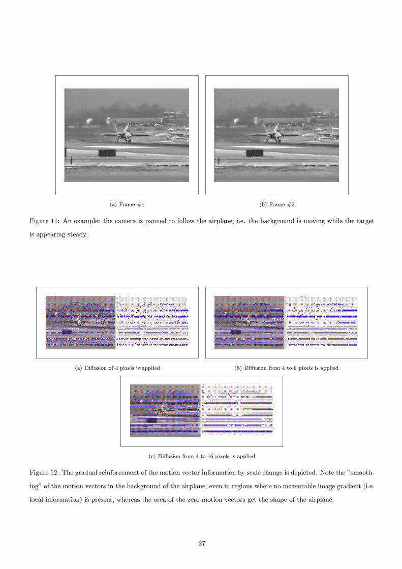
(a) Frame #1 (b) Frame #2

Figure 11: An example: the camera is panned to follow the airplane; i.e. the background is moving while the target

is appearing steady.

(a) Diffusion of 4 pixels is applied (b) Diffusion from 4 to 8 pixels is applied

(c) Diffusion from 4 to 16 pixels is applied

Figure 12: The gradual reinforcement of the motion vector information by scale change is depicted. Note the ”smooth-

ing” of the motion vectors in the background of the airplane, even in regions where no measurable image gradient (i.e.

local information) is present, whereas the area of the zero motion vectors get the shape of the airplane.

27

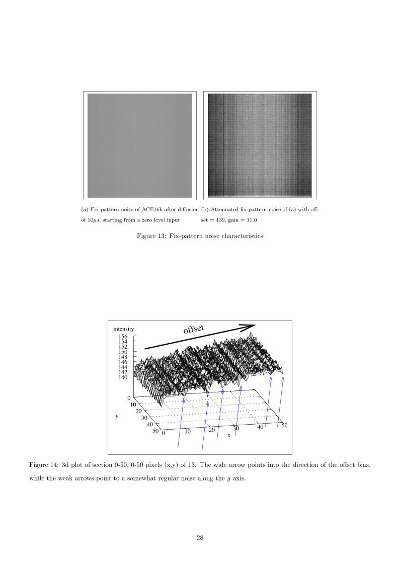
(a) Fix-pattern noise of ACE16k after diffusion

of 10µs, starting from a zero level input

(b) Attenuated fix-pattern noise of (a) with off-

set = 139, gain = 11.0

Figure 13: Fix-pattern noise characteristics

offset

x

y

140 142 144 146 148 150 152 154 156

0 10 20 30 40 50

0 10

20 30

40 50

intensity

Figure 14: 3d plot of section 0-50, 0-50 pixels (x,y) of 13. The wide arrow points into the direction of the offset bias,

while the weak arrows point to a somewhat regular noise along the y axis.

28

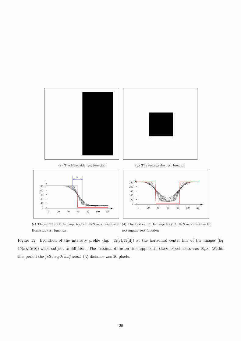
(a) The Heaviside test function (b) The rectangular test function

λ

0 20 40 60 80 100 120

0

50

100

150

200

250

(c) The evoltion of the trajectory of CNN as a response to

Heaviside test function

0 20 40 60 80 100 120

0

50

100

150

200

250

(d) The evoltion of the trajectory of CNN as a response to

rectangular test function

Figure 15: Evolution of the intensity profile (fig. 15(c),15(d)) at the horizontal center line of the images (fig.

15(a),15(b)) when subject to diffusion. The maximal diffusion time applied in these experiments was 10µs. Within

this period the full-length half-width (λ) distance was 20 pixels.

29