Analog MIMO Communication for One-shot Distributed

1

Analog MIMO Communication for One-shot

Distributed Principal Component Analysis

Xu Chen, Erik G. Larsson, and Kaibin Huang

Abstract

The ubiquitous connectivity and explosive growth of the population of edge devices motivate the

deployment of data analytics at the edge of wireless networks. They distill knowledge from enormous

mobile data to support intelligent applications ranging from e-commerce to smart cities. The fundamental

algorithm, distributed principal component analysis (DPCA), finds the most important information

embedded in a distributed high-dimensional dataset by distributed computation of a reduced-dimension

data subspace, called principal components (PCs). In this paper, to support one-shot DPCA in a wireless

system, we propose a framework of analog MIMO transmission, which features the uncoded analog

transmission of locally estimated PCs from multiple devices to a server for estimating the global PCs. To

cope with channel distortion and noise, two designs of the maximum-likelihood (global) PC estimator are

presented corresponding to the cases with and without receive channel state information (CSI). The first

design, termed coherent PC estimator, is derived by solving a Procrustes problem of subspace variable

optimization. The result reveals the form of regularized channel inversion where the regulation attempts

to alleviate the effects of both channel noise and data noise resulting from limited local datasets. The

second one, termed blind PC estimator, is designed based on the subspace channel-rotation-invariance

property and computes a centroid of the projections of received local PCs onto a Grassmann manifold.

Using the manifold-perturbation theory, the performance of both estimators is analyzed by deriving

tight bounds on the mean square subspace distance (MSSD) from global PCs to their ground truth. The

results reveal simple scaling laws of MSSD with respect to different system parameters such as device

population, data and channel signal-to-noise ratios (SNRs), and array sizes. More importantly, the scaling

laws are found to be identical for both estimator designs except for a multiplicative factor of two. This

suggests the dispensability of channel estimation to accelerate DPCA, which is validated by simulation.

Furthermore, simulation results demonstrate that to achieve the same DPCA error performance, the

X. Chen and K. Huang are with the Department of Electrical and Electronic Engineering, The University of Hong Kong,

Hong Kong (Email: {chenxu, huangkb}@eee.hku.hk). E. G. Larsson is with the Department of Electrical Engineering (ISY),

Linkoping University, 58183 Linkoping, Sweden (Email: {erik.g.larsson}@liu.se). Corresponding author: K. Huang.

November 5, 2021 DRAFT

arX

iv:2

111.

0270

9v1

[cs

.IT

] 4

Nov

202

1

2

latency of the proposed analog MIMO can be more than tenfold lower than that of the conventional

digital MIMO designs.

I. INTRODUCTION

Mobile devices have become a dominant platform for Internet access and mobile data traffic

has been growing at an exponential rate in the last decade. This motivates the relocation of data

analytics and machine learning algorithms originally performed in the cloud to the network edge

to gain fast access to enormous mobile data [1], [2]. The distilled knowledge and trained AI

models can support a wide-range of mobile applications [3]. Among many data-driven techniques,

principal component analysis (PCA) is a fundamental tool in data analytics that finds application

in diverse scientific fields ranging from wireless communication (see e.g., [4], [5]) to machine

learning (see e.g., [6], [7]). This unsupervised learning technique provides a simple way to

identify a low-dimensional subspace, called principal components (PCs), that contains the most

important information of a high-dimensional dataset, thereby facilitating feature extraction and

data compression [8]. Specifically, the principal components are computed by singular value

decomposition (SVD) of the data matrix comprising data samples as its columns [9]. In a mobile

network with distributed data, data uploading from edge devices (e.g., sensors and smartphones)

for centralized PCA may not be feasible due to the issues of data privacy and ownership and

uplink traffic congestion [10]. This issue has motivated researchers to design distributed PCA

(DPCA) algorithms [11]. A typical algorithm, called one-shot DPCA and also considered in this

work, is to compute local PCs at each device using its local data and then upload local solutions

from multiple devices to a server for aggregation to give the global PCs, which approximate

the ground-truth solution corresponding to centralized PCA [12]–[14]. Alternatively, iterative

DPCA can be designed by distributed implementation of classic numerical iterative algorithms,

for example, approximate Newton’s method [15] and stochastic gradient descent [16], [17],

which improves the performance of one-shot DPCA at the cost of much higher communication

overhead. Fast DPCA targets latency-sensitive applications such as autonomous driving, virtual

reality, and digital twins. To accelerate one-shot DPCA in a wireless network, we propose a novel

framework of analog multiple-input-multiple-output (MIMO) transmission. Its key feature is that

each device directly transmits local PCs over a MIMO channel using uncoded linear analog

modulation, which requires no transmit channel state information (CSI). We design optimal PC

(subspace) estimators at the server for both the cases with and without receive CSI.


3

To support one-shot DPCA in a wireless system, the proposed analog MIMO scheme involves

the transmission of local PCs from each device as an uncoded and linear analog modulated

unitary space-time matrix to a server. The server uses local PCs from multiple devices, which

time-share the channel, to estimate the global PCs. The scheme reduces communication latency

in three ways: 1) the coding and decoding is removed; 2) CSI feedback is unnecessary since

transmit CSI is not required; and 3) blind detection can avoid the need for explicit channel

estimation. Like its digital counterpart, analog MIMO also uses antenna arrays to spatially

multiplex data symbols but there is a distinctive difference. The symbols transmitted by the

classic digital MIMO form parallel data streams, which are separately modulated, encoded and

allocated different transmission power [18]. Thereby, the channel capacity is achieved without bit

errors. In contrast, analog MIMO is an uncoded joint source-and-channel transmission scheme

customized for DPCA. The lack of coding exposes over-the-air signals to channel noise, which,

however, can be coped with in two ways. First, the server’s aggregation of local PC from multiple

devices suppresses not only data noise (i.e., deviation from the ground-truth) but also channel

noise, which diminishes as the number of devices grows [19]. Second, the channel noise can be

suppressed by optimal PC estimation, which is a main topic of this work.

The proposed analog MIMO for DPCA shares a common feature with two classic MIMO

schemes, namely non-coherent space-time modulation and analog MIMO channel feedback, in

that they all involve transmission of a unitary matrix over a MIMO channel. Being a digital

scheme, non-coherent space-time modulation is characterized by a space-time constellation

comprising unitary matrices as its elements [20]–[23]. The purpose of such a design is to support

non-coherent communication where no CSI is required at the transmitter and receiver. This is

made possible by the fact that the distortion of a MIMO channel does not change the subspace

represented by a transmitted flat unitary matrix [22]. The same principle is exploited in this

work to enable blind detection. The capacity-achieving constellation design was found to be one

that solves the packing problem on a Grassmannian manifold, referring to a space of sub-spaces

(or equivalently unitary matrices) [20]. On the other hand, the transmitted unitary matrix in the

scenario of analog MIMO channel feedback is a pilot signal known by the receiver; its purpose is

to assist the receiver to estimate the MIMO channel for forward-link transmission assuming the

presence of channel duality [24], [25]. The scheme is found to be more efficient than digital CSI

feedback, which quantizes and transmits CSI as bits, especially in a multi-user MIMO system

where multi-user CSI feedback causes significant overhead [25]. Despite the above common


4

feature, the current analog MIMO scheme differs from the other two in comparison. Unlike

analog MIMO channel feedback, the current analog MIMO is for data transmission instead

of channel estimation. On the other hand, a unitary matrix transmitted by the analog MIMO

is directly the payload data while that using the non-coherent space-time modulation needs

demodulation and decoding into bits that represent a quantized version of the source data.

In designing analog MIMO, we assume a latency critical DPCA application where CSI feed-

back is difficult and consider both the cases with and without receive CSI. The key component of

the analog MIMO scheme is the global PC estimator that is referred to simply as PC estimator.

The designs associated with the cases with and without receive CSI are termed coherent and

blind PC estimators, respectively. The main contributions made by this work are summarized as

follows.

• Optimal PC Estimation: Given received local PCs, the optimal PC estimator is designed

based on the maximum likelihood (ML) criterion. First, the problem of optimal coherent

PC estimation is solved in closed form by formulating it as a Procrustes problem. The

resultant optimal estimator is characterized by regularized channel inversion that balances

the suppression of data and channel noise. On the other hand, to design the optimal blind PC

estimator, the knowledge of channel distribution is leveraged to transform the corresponding

ML problem into one that is solved by finding the centroid of the received local PCs by

their projection onto a Grassmannian. Theoretical analysis shows that both estimates are

unbiased.

• Estimation Error Analysis: Measured by the metric of mean square subspace distance

(MSSD) with respect to the ground-truth, the performance of the preceding designs of

optimal PC estimators is analyzed by deriving upper bounds on their MSSD using manifold

perturbation theory as a tool. The two bounds, which are tight as verified by simulation,

are observed to have the same form except for a difference by a multiplicative factor of

two. As a result, the two estimators are characterized by identical scaling laws, showing

the dispensability of receive CSI and the effectiveness of blind estimation for DPCA.

In particular, the estimation error is inversely proportional to the number of devices (or

equivalently, the global data size), achieving the same scaling as in the ideal case without

channel noise [12], [13]. Furthermore, given a fixed number of PCs, the error is a monotone

decreasing function of the data and channel signal-to-noise ratios (SNRs) and the array sizes.

It is observed that the spatial diversity gain contributed by arrays suppresses channel noise


5

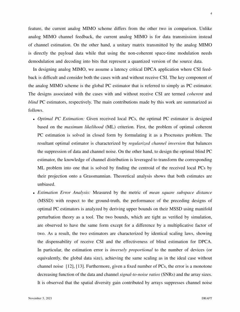
Edge Devices Edge Server

···

Local PCA

Uk = U + Zk Applications

Global PC Estimate U

Analog MIMO transmission

Data collection and computation

Analog Linear Modulation

Global PC Estimation

Analog signalYk = HkUk + Wk

CSICoherent

Blind

Fig. 1. DPCA enabled by analog MIMO communication.

more significantly than data noise. As a result, when large arrays are deployed for analog

MIMO, data noise becomes the performance bottleneck of DPCA.

In addition, simulation results demonstrate that analog MIMO can achieve much shorter

communication latency than its digital counterpart given similar error performance. Finally, it

is also worth mentioning that the current design and analytical results can be extended to the

case with transmit CSI where analog modulation facilitates over-the-air aggregation of local PCs

simultaneously transmitted by devices, further reducing multi-access latency [26]. The extension

is straightforward since channel inversion at transmitters as required by the scheme removes

MIMO channel distortion.

The remainder of the paper is organized as follows. Section II introduces system models

and metrics. The designs and performance analysis of coherent and blind global PC estimation

are presented in Section III and IV, respectively, assuming the matching of PCs’ and transmit

array’s dimensionality. The assumption is relaxed in Section V. Numerical results are provided

in Section VI, followed by concluding remarks in Section VII.

II. MODELS AND METRICS

As illustrated in Fig. 1, we consider a MIMO system for supporting DPCA over K edge devices

and coordinated by an edge server. Relevant models and metrics are described as follows.

A. Distributed Principal Component Analysis

To model DPCA, it is useful to first consider centralized PCA over L independent and iden-

tically distributed (i.i.d.) data samples xk,l ∈ RN×1, l = 1, 2, ..., L. The PCs, an M -dimensional

subspace, can be represented using a fat orthonormal matrix U ∈ RM×N with M < N since


6

the span of its row space, span(U), specifies the PCs. Then centralized PCA is to find U that

provides the best representation of the data covariance by solving the following optimization

problem:

minU

1

KL

K∑k=1

L∑l=1

∥∥xk,l −U>Uxk,l∥∥22,

s.t. UU> = IM .

(1)

It is well known that the optimal solution, denoted as U?, for (1) is given by the M dominant

eigenvectors of the sample covariance matrix R = 1KL

∑Kk=1

∑Ll=1 xk,lx

>k,l [9]. Some relevant,

useful notation is introduced as follows. Given an M -by-M real positive semidefinite symmetric

matrix M and its eigenvalue decomposition M = QMΣMQ>M, the dominant M -dimensional

eigenspace can be represented by the orthonormal matrix SM (M) = [q1,q2, ...,qM ]>, where qi

is the i-th column of QM. Using the notation allows the PCs to be written as SM (R). Next,

DPCA differs from its centralized counterpart mainly in that the L samples are distributed over

the devices. The local PCs at each device, say Uk at device k, are computed also using eigenvalue

decomposition but based on the local dataset. Due to the reduced dataset, Uk deviates from the

ground-truth U? and the deviation is modeled as additive noise, termed data noise, following a

common approach in the literature [27]–[29]: Uk = U? + Zk, where {Zk}, which model data

noise, are i.i.d. Gaussian N (0, σ2d) random variables. The data SNR, denoted as γd, is defined

as the ratio between the average power of desired data U, i.e. E [‖U‖2F ] /N = M/N , and the

data noise variance:

γd =M

Nσ2d. (2)

B. Modelling Analog MIMO Communication

First, the transmission and channel models for analog MIMO communication are described

as follows. Let Nr and Nt with Nr ≥ Nt denote the numbers of antennas at the edge server

and each device, respectively. The MIMO channel gain is denoted by Hk ∈ CNr×Nt with entries

being i.i.d. complex Gaussian CN (0, 1). For ease of notation and exposition, Nt is assumed to

be identical to the PC dimensions, M ; and this assumption is relaxed in Section V. Devices

time-share the channel to transmit an orthonormal matrix representing their local PCs, {Uk},

which is called a matrix symbol and occupies a single symbol slot. The channel remains constant

within a symbol slot but varies over slots. Consider the transmission of an arbitrary device, say


7

device k. Given no transmit CSI, the symbol, Uk, is transmitted using linear analog modulation

as in non-coherent MIMO [20]. As a result, the server receives the matrix Yk given as

Yk = HkUk + Wk = Hk (U + Zk) + Wk, (3)

and Wk ∈ CNr×N indicates channel noise with i.i.d. complex Gaussian CN (0, σ2c ) elements.

The average power of each transmitted matrix symbol is

P = E[‖Uk‖2F ]/N =(M +MNσ2

d

)/N =

(M +M2/γd

)/N.

Then let γc denote the channel SNR defined as

γc =P

σ2c

=M +M2/γd

Nσ2c

. (4)

Since each matrix symbol is real but the channel is complex, the server obtains two observations

of the transmitted symbol from each received symbol. It is useful to separate the real and

imaginary parts of the received symbol, Yk, denoted as YRek and YIm

k , respectively. They can be

written as

YRek = <{Yk} = HRe

k (U + Zk) + WRek ,

YImk = ={Yk} = HIm

k (U + Zk) + WImk ,

where HRek and HIm

k represent the real and imaginary parts of the channel and are both distributed

with i.i.d. Gaussian N (0, 1/2) entries, and WRek and WIm

k are similarly defined with i.i.d.

Gaussian N (0, σ2c/2) entries. Using the notation allows the following alternative expressions

of the received matrix symbol:

Yk =√

2

YRek

YImk

,=√

2

HRek

HImk

(U + Zk) +√

2

WRek

WImk

,4= Hk (U + Zk) + Wk. (5)

Next, consider the PC estimation at the receiver. For the case with receive CSI, the receiver is

assumed to have perfect knowledge of the channel matrix Hk and channel SNR γc by accurate

channel estimation as well as the data SNR γd from the statistics of historical data. Then such

knowledge is not available in the other blind case. Both the coherent PC estimator in the former


8

case and the blind one in the latter are designed using the ML criterion. In the presence of channel

and data noise following from isotropic Gaussian distributions, the ML based estimation can be

equivalently interpreted as linear regression fit using a least squares approximation, which could

provides a heuristic way to estimate the ground-truth (see Section IV).

Let L(U; Yk) denote the likelihood function of the estimate U given the observations in Yk.

Then the PC estimation can be formulated as

maxUL(U; Yk),

s.t. UU> = IM .

(6)

The problem is solved in the following sections to design coherent and blind PC estimators. A

key property that underpins both the current analog MIMO as well as non-coherent MIMO is

that the subspace represented by a transmitted matrix, say Uk, is invariant to a MIMO channel

rotation, which can be mathematically described as [30]

SM(U>k H>k HkUk

)= SM

(U>k Uk

). (7)

C. PC Error Metric

The PC estimation aims at estimating a subspace containing the ground-truth PCs but their

particular orientations within the subspace is irrelevant. In view of this fact, it is most convenient

to consider a Grassmann manifold, also called a Grassmannian and referring to a space of

subspaces, since a subspace appears as a single point in the manifold [30]. Let GN,M denote a

Grassmannian comprising M -dimensional subspaces embedded in an N -dimensional space. For

convenience, a point in GN,M is commonly represented using an orthonormal matrix, say U.

However, it should clarified that the point more precisely corresponds to span (U) and hence the

set of subspaces, {U′}, which satisfy the equality, span(U) = span (QU′), for some M ×M

orthonormal matrix Q. It follows from the above discussion that a suitable PC distortion metric

should measure the distance between two points in the Grassmannian, which correspond to the

subspaces of the estimated PCs and their ground-truth. Among many available subspace distance

measures, the Euclidean subspace distance, which is adopted in this work, is a popular choice

for its tractability [12], [30]. Using this metric and with the estimated PCs represented by the

orthonormal matrix U, its distance to the ground-truth U can be defined as

d(U, U) =∥∥∥U>U−U>U

∥∥∥F. (8)


9

Its geometric meaning is reflected by the alternative expression in terms of the principal angles

between the subspaces spanned by U and U, denoted as {θi}Mi=1. Define the diagonal matrix

Θ(U, U) = diag (θ1, θ2, ..., θM) for those angles; then d(U, U) =√

2∥∥∥sin Θ(U, U)

∥∥∥F

[12].

Building on the subspace distance measure, we define the PC error metric as follows.

Definition 1 (Mean square subspace distance). The mean square subspace distance (MSSD)

between U and U is defined as

dms(U, U) = E[d2(U, U)

]= 2M − 2E

[Tr(U>UU>U)

]. (9)

where the expectation is taken over the distributions of data noise Z, channel noise W, and also

channel gain H in the case of blind PC estimation.

III. PC ESTIMATION FOR COHERENT MIMO RECEIVERS

A. Design of Coherent PC Estimator

First, the usefulness of receive CSI is to facilitate coherent combination of the received data.

To this end, channel inversion is applied to a received matrix symbol, say Yk, by multiplication

with the zero-forcing matrix, H+k

4= (H>k Hk)

−1H>k , which is the pseudo inverse of the channel

Hk. Using (5), this yields the following observations for PC estimation: H+k Yk = U + Zk +

H+k Wk,∀k. The processed observations follow a matrix Gaussian distributionMN (U,Σk, IN)

with Σk = σ2dIM + σ2

c H+k

(H+k

)>. Specifically,

p(H+k Yk|U,H) =

exp(−1

2Tr(

(H+k Yk −U)>Σ−1k (H+

k Yk −U)))

(2π)MN2 det (Σk)

N2

.

Next, the ML PC estimator is derived by maximizing the likelihood function that is defined as

the joint probability of the observations {H+k Yk}Kk=1 conditioned on the ground-truth U and

channel realizations {Hk}Kk=1.

Since {H+k Yk}Kk=1 are mutually independent, the logarithm of the likelihood function can be

written as

L(U; Y, H) = ln

(K∏k=1

p(H+k Yk|U, Hk)

),

= −1

2

K∑k=1

Tr(

(H+k Yk −U)>Σk

−1(H+k Yk −U)

)− 1

2MNK ln(2π)− N

2

K∑k=1

ln det (Σk) .


10

One can observe from the above expression that the variable U only enters into the first term

which can be further expanded as:

− 1

2

K∑k=1

Tr(Y>k (H+

k )>Σ−1k H+k Yk + U>Σ−1k U− 2U>Σ−1k H+

k Yk

)=

K∑k=1

Tr(U>Σ−1k H+

k Yk

)− 1

2

K∑k=1

Tr(Y>k (H+

k )>Σ−1k H+k Yk + Σ−1k

).

It follows that the likelihood function is determined by U through∑K

k=1 Tr(U>Σ−1k H+

k Yk

).

This allows the ML problem in (6) to be particularized for the current case as

maxU

1

K

K∑k=1

Tr(U>Σ−1k H+

k Yk

),

s.t. UU> = IM .

(10)

The problem in (10) is non-convex due to the feasible region restricted to a hyper-sphere.

One solution method is to transform it into an equivalent, tractable orthogonal Procrustes prob-

lem [31]. To this end, consider the following SVD

J =1

K

K∑k=1

Σ−1k H+k Yk = UJΛJV

>J , (11)

where the diagonal matrix ΛJ = diag (λJ,1, ..., λJ,M) with λJ,m representing the m-th singular

value, and UJ and V>J are orthonormal eigen matrices. Let them be expressed in terms of the

singular vectors of J: UJ = [uJ,1, ...,uJ,M ], V>J = [vJ,1, ...,vJ,M ]>. Let U? denote the optimal

solution for the problem in (10), which yields the optimal estimate of the ground-truth U.

Then substituting (11) into the objective function in (10) allows U? to be given as

U? = arg maxU∈GN,M

Tr(U>J

),

= arg maxU∈GN,M

Tr(U>UJΛJV

>J

),

= arg maxU∈GN,M

M∑m=1

λJ,m ·⟨U>uJ,m,vJ,m

⟩.

The above problem can be solved using the fact that∑M

m=1 λJ,m ·⟨U>uJ,m,vJ,m

⟩≤∑M

m=1 λJ,m

with equality when U>uJ,m = vJ,m,∀m. It follows that U∗>UJ = VJ, or equivalently U? =

UJV>J . Using [32, Theorem 7.3.1], UJV

>J can be obtained from the polar decomposition of

the matrix summation J in (11), i.e., UJV>J = (JJ>)−1/2J, and furthermore spans the same

principal eigenspace as span(V>J). This leads to the following main result of this sub-section.


11

Theorem 1 (Optimal PC Estimation with Receive CSI). Given the channel matrices {Hk}Kk=1

and the received matrix symbols {Yk}Kk=1, the optimal global PCs based on the ML criterion

are given as

U? = SM(J>J

), (12)

where J = 1K

∑Kk=1

[σ2

dIM + σ2c H

+k (H+

k )>]−1

H+k Yk.

Theorem 1 suggests that the optimal coherent PC estimator should 1) first coherently combine

received observations with weights reflecting a linear minimum-mean-square error (MMSE)

receiver and 2) then compute the dominant singular space of the result, yielding the optimal

estimate of the ground-truth PCs. The weights that aim at coping with MIMO channels and

noise distinguish the current DPCA over wireless channels from the conventional designs where

weights are either unit [12] or independent of channels [13], [33].

Remark 1 (Data-and-Channel Noise Regularization). As shown in Theorem 1, the zero-forcing

matrix H+k is used to equalize the channel distortion but by doing so, it may amplify channel

noise given a poorly conditioned channel. This issue is addressed by a regularization term,[σ2

dIM + σ2c H

+k (H+

k )>], that balances data and channel noise based on the knowledge of their

covariance matrices.

Last, the PC estimation in Theorem 1 is unbiased as shown below.

Corollary 1. The coherent PC estimator in Theorem 1 together with the preceding channel

inversion achieves unbiased estimation of the global PCs in the following sense. Define J = E [J]

with J given by Theorem 1, and the optimal PC estimate U? = SM(J>J

). Then d

(U?,U

)= 0.

Proof. According to (11), the J is given by

J = E

[1

K

K∑k=1

[σ2dIM + σ2

c H+k (H+

k )>]−1H+k Yk

],

= E[[σ2

dIM + σ2c H

+k (H+

k )>]−1]

U, .

Define C4= E

[[σ2

dIM + σ2c H

+k (H+

k )>]−1]

and clearly rank (C) = M . Then, based on the

property in (7), we have SM(U>C>CU

)= SM

(U>U

)which completes the proof.

The above result also implies that as the number of devices, K, increases (so does the global

data size), the optimal estimate U? in Theorem 1 converges to the ground-truth since J→ J.


12

B. Error Performance Analysis

The performance of the optimal coherent PC estimation in the preceding sub-section can be

analyzed using a result from perturbation theory for Grassmann manifolds. To this end, consider

two perturbed subspaces V1 = SM(G>1 G1

)and V2 = SM

(G>2 G2

), where G1 = F + εE1 and

G2 = F + εE2 with the orthonormal matrix F ∈ GN,M representing a ground-truth, εEi, i = 1, 2

denoting random additive perturbations, and ε > 0 controlling the perturbation magnitude. The

following result is from [34, Theorem 9.3.4].

Lemma 1. The squared subspace distance of the perturbed subspaces V1 and V2 satisfies

d2(V1,V2) = 2ε2Tr(∆EF⊥>F⊥∆E

>) +O(ε3), (13)

where F⊥ is the orthogonal complement of F and ∆E = E1 − E2.

Using Lemma 1, it is proved in Appendix A that the PC estimation error can be characterized

as follows.

Lemma 2. The square error of the optimal PC estimate U? in Theorem 1 is

d2(U?,U) = 2Tr(∆EU⊥>U⊥∆E

>) +O(‖Σ−1E ‖

3F

), (14)

where ∆E ∼ MN[0,Σ−1E , IN

]with ΣE =

∑Kk=1(σ

2dIM + σ2

c H+k (H+

k )>)−1 and U⊥ is the

orthogonal complement of U.

Based on the definition of ΣE, one can infer that the residual term O(‖Σ−1E ‖3F

)in Lemma 2

diminishes as the number of devices (or the global data size) K →∞ or data noise and channel

noise σd, σc → 0. Then using Lemma 2 with the residual term omitted, the error of optimal PC

estimation can be characterized as follows.

Theorem 2 (Error of Optimal Coherent PC Estimation). Given many devices (K → ∞) and

small channel and data noise (σd, σc → 0), the MSSD of the optimal coherent PC estimator in

Theorem 1 can be asymptotically upper bounded as

dms(U?,U) ≤ 2M(N −M)

K

(σ2

d +1

2Nr −M − 1σ2

c

), (15)

for a MIMO system (i.e., 2Nr −M > 1).

Proof. See Appendix B.


13

Note that as M increases, the first term in the MSSD upper bound in (15), 2M(N−M)K

, grows if

M ≤ N2

but otherwise decreases. This is due to the following well known property of a random

point (subspace) uniformly distributed on a Grassmannian. Its uncertainty (and hence estimation

error) grows with its dimensionality M , reaches the maximum at M = N2

, and reduces afterwards

since it can be equivalently represented by a lower-dimensional complementary subspace [20].

Next, the MSSD upper bound can be rewritten in terms of the channel and data SNRs given in

(2) and (4) as

dms(U?,U) ≤ 2M2(N −M)

KN

[γ−1d + (1 +Mγ−1d )γ−1c ·

1

2Nr −M − 1

]. (16)

It is observed from (16) that given fixed data and channel SNRs, the estimation error increases

with M and reaches a peak at M = 2N/3 instead of M = N/2 when noise variances are fixed.

Based on Theorem 2, the effects of different system parameters on the error performance of

coherent PC estimation are described as follows.

• The MSSD linearly decays as the device number K, or equivalently the number of noisy

observations of the global PCs, increases. The scaling law is identical to that for conventional

DPCA over reliable links (see, e.g. [12] and [13]). The result suggests increasingly accurate

estimation of the ground-truth global PCs as more devices participate in DPCA.

• The result in (16) shows a trade-off between the data and channel noise. Furthermore, if

channel noise is negligible, one can observe from (16) that the estimation error diminishes

about inversely with increasing data SNR, namely O(

2M2

Kγd

)if N � M . On the other

hand, if channel noise is dominant, the error decays with increasing channel SNR as

O(

1(2Nr−Nt−1)γc

). The factor 2Nr −Nt − 1 is contributed by spatial diversity gain of using

a large receive array with Nr elements.

IV. PC ESTIMATION FOR BLIND MIMO RECEIVERS

In the last section, an optimal coherent estimator was designed for PC estimation with receive

CSI. The requirements on receive CSI and data statistics, say data SNR, are relaxed in this

section so as to obviate the need of channel estimation and feedback, yielding the current case

of blind PC estimation.

A. Integrated Design of Blind PC Estimator

1) Approximating the ML Problem: The lack of receive CSI complicates the ML problem

in (6). It is made tractable by finding a tractable lower bound on the likelihood function, which


14

is the objective, as follows. To this end, as the unknown channel is a Gaussian random matrix,

the distribution of a received matrix symbol, say Yk, conditioned on the ground truth U can be

written as

p(Yk|U) = EZk[p(Yk|U,Zk)],

= EZk

[1

(2π)NrNdet(Σ′k)Nr

exp

(−1

2Tr(Yk(Σ

′k)−1Y>k

))], (17)

where we recall Zk to be the data noise and define Σ′k = σ2c IN + (U + Zk)

>(U + Zk).

Next, as received symbols are mutually independent, the likelihood function is given as

L(U; Y) = ln

(K∏k=1

p(Yk|U)

),

=K∑k=1

ln(EZk

[p(Yk|U,Zk)

]). (18)

It can be lower bounded using the Jensen’s inequality as L(U; Y) ≥ Llb(U; Y) with

Llb(U; Y) =K∑k=1

EZk

[ln(p(Yk|U,Zk)

)],

=K∑k=1

EZk

[−1

2Tr(Yk(Σ

′k)−1Y>k

)−Nr ln (det(Σ′k))

]−NrNK ln (2π) . (19)

For tractability, we approximate the objective of the ML problem in (18) by its lower bound

in (19). The new objective can be further simplified using the following result.

Lemma 3. Only the first term of Llb(U; Y) in (19), i.e.,∑K

k=1 EZk

[−1

2Tr(Yk(Σ

′k)−1Y>k

)],

depends on the ground truth U.

Proof. See Appendix C.

Using the above result and changing the sign of its objective, the ML problem in (6) can be

approximated as the following minimization problem

minU

1

K

K∑k=1

EZk

[Tr(Yk(Σ

′k)−1Y>k

)],

s.t. UU> = IM .

(20)

The above ML problem is not yet tractable and requires further approximation of its objective.

For ease of exposition, represent its summation term as Ψk = EZk

[Tr(Yk(Σ

′k)−1Y>k )

]. Some

useful notations are introduced as follows. Define a Gaussian matrix Zk = [IM 0M,N−M ]+ZkQ>


15

that is a function of data noise (see Appendix D) and independent over k. Let Pk = SM(Z>k Zk)>,

which denotes an orthonormal matrix representing the principal M -dimensional column subspace

of Zk, and Sk denote its singular value matrix.

Lemma 4. The term Ψk defined earlier can be rewritten as

Ψk = C − σ−2c EPk,Sk

[Tr(YkQ

>PkΛSkP>k QY>k

)], (21)

where the constant C = σ−2c Tr(YkY

>k

), the diagonal matrix ΛSk

= S2k

(σ−2c IM + S2

k

)−1, and

Q =[U>

(U⊥)>]>.

Proof. See Appendix D.

Note that C is independent of the ground truth U. Therefore, it follows from Lemma 4 that the

maximization of Ψk can be approximated by minimizing EPk,Sk

[Tr(YkQ

>PkΛSkP>k QY>k

)].

In other words, the current ML problem is equivalent to:

maxU

1

K

K∑k=1

EPk,Sk

[Tr(YkQ

>PkΛSkP>k QY>k

)],

s.t. UU> = IM .

(22)

2) Optimization on Grassmannian: The above problem is solved using the theory of opti-

mization on Grassmannian, involving the optimization of a subspace variable, as follows. To this

end, decompose the space of a received matrix symbol, say Yk, by eigen-decomposition as

Y>k Yk = U>Yk

Λdat,kUYk+ V>

YkΛnoi,kVYk

.

The eigenspace represented by UYkis the data space while that by VYk

is the channel-noise

space. Here, each summation term Tr(YkQ

>PkΛSkP>k QY>k

)directly depends on how close

the PCs, say P>k Q, is to that of Y>k Yk, i.e. UYk. Specifically, we have

Tr(YkQ

>PkΛSkP>k QY>k

)≤ Tr

(Λnoi,kΛSk

),

where the upper bound is achieved if d(Q>Pk,UYk) = 2M − 2Tr

(UYk

Q>PkP>k QU>

Yk

)= 0.

Therefore, we replace each trace term by the simplified term Tr(UYk

Q>PkP>k QU>

Yk

)that

focuses on projections onto a Grassmannian.

It follows that the ML problem in (22) can be approximated as

maxU

1

K

K∑k=1

EPk

[Tr(UYk

Q>PkP>k QU>

Yk

)],

s.t. UU> = IM .

(23)


16

To facilitate optimization on Grassmannian, we can rewrite the objective in terms of subspace

distance as

1

K

K∑k=1

EPk

[Tr(UYk

Q>PkP>k QU>

Yk

)]=

1

K

K∑k=1

Tr(Q>EPk

[PkP

>k

]QU>

YkUYk

),

where the expectation EPk

[PkP

>k

]shows the following property.

Lemma 5. The orthogonal projection matrix PkP>k ’s expectation is diagonal, say EPk

[PkP

>k

]=

Λµ = diag (µ1, µ2, ..., µN) with µi ≥ 0, i ∈ {1, 2, ..., N}.

Proof. See Appendix E.

Based on Lemma 5, define the summation J′ = 1K

∑Kk=1 U>

YkUYk

and the ML problem in (22)

is written asmaxU

Tr(Q>ΛµQJ′

),

s.t. UU> = IM .

(24)

Although the problem shown in (24) is non-convex due to the orthonormal constraint, there still

is a closed-form solution serving as the PC estimator for the blind case. To this end, define the

SVD: J′ = UJ′ΛJ′U>J′ with U>J′ = SN (J′). As the matrix J′ is positive semidefinite, the entries

of ΛJ′ are non-negative and we have the following upper bound on the objective function (24):

Tr(Q>ΛµQJ′

)= Tr

((QUJ′)>ΛµQUJ′ΛJ′

),

≤ Tr (ΛµΛJ′) .

The equality is achieved when Q = UJ′ . It follows that the M -dimensional principal eigenspace

of J′, SM (J′), is the optimal solution for the problem in (24).

Theorem 3 (ML based PC estimation without receive CSI). Given the received matrix symbols

{Yk}Kk=1 and the blind PC estimator based on ML criterion is given by

U? = SM (J′) , (25)

where J′ = 1K

∑Kk=1 U>

YkUYk

and UYk= SM

(Y>k Yk

).

The optimal blind PC estimation in Theorem (3) essentially consists of three steps: 1) project-

ing each received matrix symbol to become a single point on the Grassmannian; 2) compute the

centroid by averaging the points in the Euclidean space; 3) then projecting the result onto the


17

Grassmannian to yield the estimated global PCs. It should be emphasized that Step 1) leverages

the rotation-invariant property of analog subspace transmission in (7). On the other hand, the

centroid computation in Sep 2) is an aggregation operation that suppresses both the data and

channel noise. The aggregation gain grows as the number of devices or equivalently the number

of observations grow as quantified in the next sub-section.

Remark 2 (Geometric Interpretation). The result in Theorem 3 can be also interpreted geo-

metrically as follows. According to (8), each summation term in the objective function in (24)

measures the subspace distance between a received matrix symbol and a Gaussian matrix, where

the latter’s PCs are uniformly displaced by Q on the Grassmannian. Since the Gaussian matrix

is isotropic and its mean’s PCs coincides with U after being displaced by Q, we can obtain an

equivalent geometric form of the problem in (24) as

minU

1

K

K∑k=1

d2(U,UYk),

s.t. UU> = IM .

The above problem is to identify the optimal U such that the sum over its square distance to

each signal’s PCs is minimized. Its optimal solution, as proved in the literature is the centroid of

signal PCs on the Grassmannian (see, e.g. [12]), which is aligned with the result in the theorem.

Finally, the the blind ML PC estimator in Theorem 3 yields an unbiased estimate of the

ground-truth as proved below.

Corollary 2. The blind PC estimator in Theorem 3 computing the centroid of received noisy

observations achieves unbiased estimation of the global PCs in the following sense. Define

J′ = E [J′] with J′ follows that in Theorem 3, and the optimal PC estimate U? = SM(J′). Then

d(U?,U) = 0.

Proof. See Appendix F.

B. Optimality of Symbol-by-Symbol Blind PC Detection

The blind estimator designed in the preceding sub-section performs joint detection of a block

of received symbols. However, its aggregation form in Theorem 3, which results from i.i.d.

channel and Gaussian noise over users, suggests the optimality of detecting the subspaces of

individual symbols followed by applying the conventional aggregation method for DPCA [12],


18

[13]. The conjecture is corroborated in the sequel by designing the single-symbol blind PC

detector under two different criteria.

First, consider the ML criterion. Conditioned on the transmitted symbol Uk and similarly as

(17), the distribution of Yk is obtained as

p(Yk|Uk) =exp

(−1

2Tr(Y>k

(σ2

c IN + U>k Uk

)−1Yk

))(2π)NrNdet

(σ2

c IN + U>k Uk

)Nr,

=1

(2πσ2c )NrN (1 + σ−2c )NrM

exp

(− 1

2σ2cTr(Y>k Yk − (1 + σ2

c )−1Y>k U>k UkYk

)).

The above result shows that the distribution depends on Uk through the term Tr(Y>k U>k UkYk

).

Therefore, the optimal ML estimate of Uk can be obtained by solving the following problem:

minUk

Tr(Y>k U>k UkYk

),

s.t. UkU>k = IM .

(26)

Note that even though Uk is not orthonormal, the orthonormal constraint in the above problem

serves the purpose of matched filtering by reducing the noise dimensionality. Define UYk=

SM(Y>k Yk). The problem in (26) has the optimal solution: U?k = QMUYk

with QM is an

arbitrary M ×M orthonormal matrix. Equivalently, span(U?k) = span(UYk

).

Second, in the absence of channel noise, the detection problem can be formulated as linear

regression: Yk = HkUk where Hk and Uk denote the estimates of channel and transmitted

subspace, respectively. The resultant regression error can be measured as ‖Yk − HkUk‖2. Then

the problem of minimizing the regression error can be solved by two steps: 1) given any Uk,

the optimal Hk is given by H?k = arg minHk

‖Yk − HkUk‖2 = YkU>k ; 2) given the optimal

H?k, the optimal Uk is given by U?

k = arg minUkU>k =IM

‖Yk − YkU>k Uk‖2 = QMUYk

. One

can observe the result to be identical to the preceding ML counterpart.

Finally, by setting the arbitrary orthonormal matrix QM to be an identity matrix, the aggre-

gation of subspaces estimated from individual received symbols using the above single-symbol

detector yields an identical result as in Theorem 3.

C. Error Performance Analysis

As before, the error performance of blind PC estimation is also analyzed based on the result

in Lemma 1. As the UYkin the derived estimator (see Theorem 3) does not directly admit

tractability, an approximation is necessary. Consider a symbol resulting from applying channel


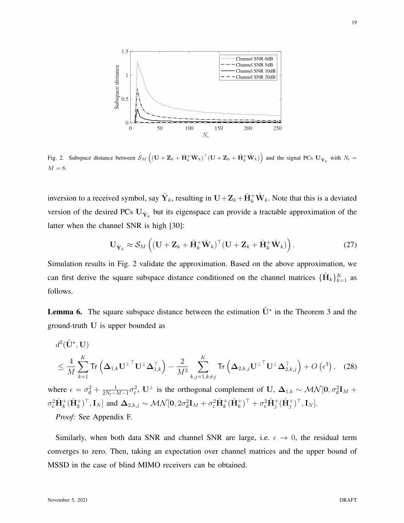
19

0 50 100 150 200 2500

0.5

1

1.5

Subsp

ace

dis

tance

Channel SNR 0dB

Channel SNR 5dB

Channel SNR 10dB

Channel SNR 20dB

Fig. 2. Subspace distance between SM

((U+ Zk + H+

k Wk)>(U+ Zk + H+

k Wk))

and the signal PCs UYkwith Nt =

M = 8.

inversion to a received symbol, say Yk, resulting in U+Zk+H+k Wk. Note that this is a deviated

version of the desired PCs UYkbut its eigenspace can provide a tractable approximation of the

latter when the channel SNR is high [30]:

UYk≈ SM

((U + Zk + H+

k Wk)>(U + Zk + H+

k Wk)). (27)

Simulation results in Fig. 2 validate the approximation. Based on the above approximation, we

can first derive the square subspace distance conditioned on the channel matrices {Hk}Kk=1 as

follows.

Lemma 6. The square subspace distance between the estimation U? in the Theorem 3 and the

ground-truth U is upper bounded as

d2(U?,U)

≤ 4

M

K∑k=1

Tr(∆1,kU

⊥>U⊥∆>1,k

)− 2

M2

K∑k,j=1,k 6=j

Tr(∆2,k,jU

⊥>U⊥∆>2,k,j

)+O

(ε3), (28)

where ε = σ2d + 1

2Nr−M−1σ2c , U⊥ is the orthogonal complement of U, ∆1,k ∼ MN [0, σ2

dIM +

σ2c H

+k (H+

k )>, IN ] and ∆2,k,j ∼MN [0, 2σ2dIM + σ2

c H+k (H+

k )> + σ2c H

+j (H+

j )>, IN ].

Proof: See Appendix F.

Similarly, when both data SNR and channel SNR are large, i.e. ε → 0, the residual term

converges to zero. Then, taking an expectation over channel matrices and the upper bound of

MSSD in the case of blind MIMO receivers can be obtained.


20

Theorem 4 (Error of Proposed Blind PC Estimation). Given many devices (K →∞) and small

channel and data noise (σd, σc → 0), the MSSD of the blind PC estimator in Theorem 3 can be

asymptotically upper bounded as

dms(U?,U) ≤ 4M(N −M)

K

(σ2

d +1

2Nr −M − 1σ2

c

). (29)

Proof. See Appendix H.

Using the definition of σd and σc yields the following result:

dms(U?,U) ≤ 4M2(N −M)

KN

[γ−1d + (1 +Mγ−1d )γ−1c ·

1

2Nr −M − 1

].

Remark 3 (Coherent vs. Blind). Comparing Theorems 2 and 4, the error bounds for both the

coherent and blind PC estimators are observed to have the same form except for the difference

by a multiplicative factor of two. This shows that despite the lack of receive CSI, the latter can

achieve similar performance as its coherent counterpart mainly due to the exploitation of the

channel-rotation-invariance of analog subspace transmission in (3). On the other hand, the said

multiplicative factor represents the additional gain in estimation error suppression via regularized

channel inversion that alleviates the effects of data and channel noise.

V. EXTENSION TO PCS WITH ARBITRARY DIMENSIONS

In the previous sections, we assume Nt = M such that each matrix symbol representing local

PCs can be directly transmitted over a transmit array. The results can be generalized by relaxing

the assumption as follows.

First, consider the case of Nt ≥M . One can introduce an Nt-by-M orthonormal matrix X that

maps an M -dimensional symbol to the Nt-element array, yielding the following communication

model:

Yk = HkX(U + Zk) + Wk

4= Hk(U + Zk) + Wk,

where Hk4= HkX. With transmit CSI, X can be generated isotropically. As a result, Hk follows

an isotropic matrix Gaussian MN (0, INr , IM) and thus the results in the preceding sections

remain unchanged.


21

Next, consider the case of M > Nt. Local PCs at a device have to be transmitted as multiple

matrix symbols. Let a local estimate, say Uk, be partitioned into T M ′×N component matrices

with M ′ ≤ Nt as follows

Uk = [U>k,1,U>k,2, ...,U

>k,T ]>.

Since each component matrix contains M ′ columns of the orthonormal matrix of Uk, it is

also orthonormal. By introducing a mapping matrix X′ similarly as in the preceding case, each

component matrix, say Uk,t, can be transmitted as a single matrix symbol, resulting in

Yk,t = Hk,tX′Uk,t + Wk,t.

Obviously, if M ′ = Nt, the mapping X′ is unnecessary and the above model reduces to

Yk,t = Hk,tUk,t + Wk,t.

At the receiver, multiple received component matrices are combined into a single one in a similar

way as in (3):

Yk = [Y>k,1,Y>k,2, ...,Y

>k,T ]>

= diag (Hk,1,Hk,2, ...,Hk,T ) Uk + [W>k,1,W

>k,2, ...,W

>k,T ]>. (30)

Therefore, we can obtain a communication model differing from that in (3) only in the MIMO

channel which is block diagonal in the current case. For coherent PC estimation, it is straight-

forward to show that the design modified using the generalized channel model retains its unbi-

asedness and ML optimality. As for blind PC estimation, diag(Hk,1, ...,Hk,T ) keeps the isotropic

property as before that guarantees unbiased estimation. Furthermore, to modify the design and

analysis, the expectation EHk

[H+k (H+

k )>]

is replaced with

EHk

[H+k (H+

k )>]

= diag(EHk,1

[H+k,1(H

+k,1)>],EHk,2

[H+k,2(H

+k,2)>], ...,EHk,T

[H+k,T (H+

k,T )>]),

where Hk,t is derived from Hk,t using the method in (5). This modification, according to the

derivation process, only changes the coefficients of σ2c in both Theorem 1 and 3. Therefore, one

can conclude that the scaling laws of estimation error are preserved during the extension.

VI. SIMULATION RESULTS

The default simulation settings are as follows. The PC dimension is M = 8 and the data

dimensionality is N = 200. In the MIMO communication system, the server is equipped with

Nr = 16 antennas and each edge device with Nt = M = 8 antennas.


22

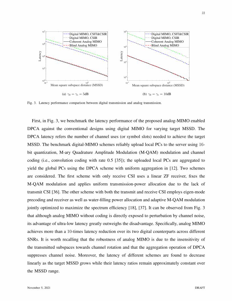
10-1

100

Mean square subspace distance (MSSD)

103

104

105

106

107

Lat

ency

Digital MIMO, CSIT&CSIR

Digital MIMO, CSIR

Coherent Analog MIMO

Blind Analog MIMO

(a) γd = γc = 5dB

10-1

100

Mean square subspace distance (MSSD)

103

104

105

106

Lat

ency

Digital MIMO, CSIT&CSIR

Digital MIMO, CSIR

Coherent Analog MIMO

Blind Analog MIMO

(b) γd = γc = 10dB

Fig. 3. Latency performance comparison between digital transmission and analog transmission.

First, in Fig. 3, we benchmark the latency performance of the proposed analog-MIMO enabled

DPCA against the conventional designs using digital MIMO for varying target MSSD. The

DPCA latency refers the number of channel uses (or symbol slots) needed to achieve the target

MSSD. The benchmark digital-MIMO schemes reliably upload local PCs to the server using 16-

bit quantization, M-ary Quadrature Amplitude Modulation (M-QAM) modulation and channel

coding (i.e., convolution coding with rate 0.5 [35]); the uploaded local PCs are aggregated to

yield the global PCs using the DPCA scheme with uniform aggregation in [12]. Two schemes

are considered. The first scheme with only receive CSI uses a linear ZF receiver, fixes the

M-QAM modulation and applies uniform transmission-power allocation due to the lack of

transmit CSI [36]. The other scheme with both the transmit and receive CSI employs eigen-mode

precoding and receiver as well as water-filling power allocation and adaptive M-QAM modulation

jointly optimized to maximize the spectrum efficiency [18], [37]. It can be observed from Fig. 3

that although analog MIMO without coding is directly exposed to perturbation by channel noise,

its advantage of ultra-low latency greatly outweighs the disadvantage. Specifically, analog MIMO

achieves more than a 10-times latency reduction over its two digital counterparts across different

SNRs. It is worth recalling that the robustness of analog MIMO is due to the insensitivity of

the transmitted subspaces towards channel rotation and that the aggregation operation of DPCA

suppresses channel noise. Moreover, the latency of different schemes are found to decrease

linearly as the target MSSD grows while their latency ratios remain approximately constant over

the MSSD range.


23

100

102

104

Number of edge device, K

10-3

10-2

10-1

100

101

102

103

Mea

n s

quar

e su

bsp

ace

dis

tance

Simulation

Upper bound

d=

c=0,5,10dB

(a) Coherent estimation

100

102

104


10-3

10-2

10-1

100

101

102

103

Mea

n s

quar

e su

bsp

ace

dis

tance

Simulation

Upper bound

d=

c=0,5,10dB

(b) Blind estimation

100

102

104


10-3

10-2

10-1

100

101

102

Mea

n s

qu

are

sub

spac

e d

ista

nce

Blind Est.

Coherent Est.

d=

c=0,5,10dB

(c) Comparison

Fig. 4. PC estimation performance comparisons for varying numbers of devices between simulation and analysis for (a) coherent

estimation and (b) blind estimation, and (c) comparison between the two designs.

Second, the effect of device population on the PC estimation is investigated. To this end, the

curves of MSSD versus the number of devices K, are plotted in Fig. 4, for which the data and

channel SNRs are set as γd = γc = {0, 5, 10} dB. The scaling laws derived in Theorems 1

and 3 are validated using simulation results in Figs. 4(a) and 4(b), for the designs of coherent

and blind PC estimation, respectively. The performance comparison between the two designs is

provided in Fig. 4(c). We observe that they follow the same linear scaling law for coherent and

blind estimation, namely that MSSD decreases linearly as K grows. Varying the SNRs shifts

the curves but does not change their slopes. Next, one can observe from Figs. 4(a) and 4(b) that

the performance analysis accurately quantifies the linear scaling and its rate. The derived MSSD

bound is tight for the case of coherent estimation and a sufficiently large number of devices (e.g.,

K ≥ 10) while for the other case of blind estimation the bound is not as tight but satisfactory.

More importantly, the performance comparison in Fig. 4(c) confirms a main conclusion from

the analysis (see Remark 3) that blind PC estimation performs only with a small gap from that

of the coherent counterpart especially at sufficiently high SNRs, advocating fast DPCA without

CSI.

Finally, the effects of data/channel SNRs on the performance of analog MIMO are character-

ized in Fig. 5 where the curves of MSSD versus data/channel SNR are plotted for K = 1000

devices. In the high channel-SNR regime, one can observe that increasing the data SNR reduces


24

10-7

10-6

0

10-5

10-4

10-3

Mea

n s

qu

are

sub

spac

e d

ista

nce

10-2

0

10-1

55

Data SNR (dB)

10

Channel SNR (dB)10

15 1520 20

Coherent Est.

(a) Coherent estimation (b) Blind estimation

Fig. 5. Mean square subspace distance versus data and channel SNR.

the MSSD of both the coherent and blind estimators at an approximately linear rate. On the other

hand, with the data SNR fixed, the MSSD is relatively insensitive to channel SNR especially

in the low data-SNR regime. This is due to the fact that the diversity gain of multiple antenna

systems suppressing channel noise and large data noise becomes dominant, which is consistent

with our analysis results shown in Theorem 2 and 4.

VII. CONCLUDING REMARKS

We have presented an analog MIMO communication framework for supporting ultra-fast

DPCA in a wireless system. Besides spatial multiplexing inherent in MIMO, the proposed

approach dramatically reduces the DPCA latency by avoiding quantization, coding, and CSI

feedback. Furthermore, by analyzing and comparing the performance of analog MIMO with and

without receive CSI, we have found that even channel estimation may not be necessary as the

resultant performance gain is small. This advocates blind analog MIMO to further accelerate

DPCA. Compared with digital MIMO, more than a tenfold latency reduction has been demon-

strated for analog MIMO in achieving the same DPCA error performance. Building on findings

in this work, we believe that analog communication will play an important role in machine

learning and data analytics at the network edge. This requires new techniques to properly control

the effects of channel distortion and noise so that they can be masked by those of data noise.

Moreover, the new techniques should be customized for the algorithms of specific applications


25

(e.g., the current principal-component estimation for DPCA) to optimize the system efficiency

and performance.

APPENDIX

A. Proof of Lemma 2

The orthonormal U? given in Theorem 1 represents the principal eigenspace of J, i.e. U? =

SM(J>J

), where J = 1

KΣEU + E with ΣE =

∑Kk=1

[σ2

dIM + σ2c H

+k (H+

k )>]−1

. Due to Zk +

H+k Wk ∼MN [0, σ2

dIM +σ2c H

+k (H+

k )>, IN ], ∀k, E follows from a matrix Gaussian distribution

MN [0,ΣE, IN ]. Note that ΣE is a positive definite Hermitian matrix and there always exists

an inverse matrix Σ−1E . Then, the rotation-invariant property of subspace in (7) gives

U? = SM((ΣEU + E)>(ΣEU + E)

)= SM

((U + Σ−1E E)>(U + Σ−1E E)

),

where Σ−1E E is matrix GaussianMN [0,Σ−1E , IN ]. Then, based on Lemma 1, set ε = C1‖Σ−1E ‖2with a constant C1, E1 = 1

εΣ−1E E and E2 = O and we can get the final result.

B. Proof of Theorem 2

Based on Lemma 2, with the second residual term omitted, the MSSD is approximated as

dms(U?,U) ≈ E

[2Tr

(∆EU⊥

>U⊥∆E

>)],

= 2(N −M)E{Hk}Kk=1

[Tr(Σ−1E

)],

≤ 2(N −M)Tr

( K∑k=1

EHk[Ak]

−1

)−1 ,

where we define Ak = σ2dIM + σ2

c H+k (H+

k )> and the last inequality comes from Jensen’s in-

equality and the fact that Tr(

(∑K

k=1 A−1k )−1)

is concave over {Ak}Kk=1 [38]. Since H+k (H+

k )> =

(H>k Hk)−1 is an inverse Wishart matrix, given 2Nr − M > 1, we have the first moment

E[(H>k Hk)−1] = 1

2Nr−M−1IM [39].

Using the above results yields the following upper bound:

dms(U?,U) ≤ 2(N −M)Tr

( K∑k=1

(σ2

d +σ2

c

2Nr −M − 1

)−1IM

)−1 ,

=2M(N −M)

K

(σ2

d +σ2

c

2Nr −M − 1

).


26

C. Proof of Lemma 3

In Llb(U; Y), the third term is constant. For the second part, we have

det(σ2

c IN + (U + Zk)>(U + Zk)

) (a)= det

(σ2

c IM + (U + Zk)(U + Zk)>) ,

= det((σ2

c + 1)IM + ZkU> + UZ>k + ZkZ

>k

),

where (a) follows from Sylvester’s determinant identity. The elements of Zk are i.i.d. Gaussian

N (0, σ2d), which means that Zk has an isotropic matrix Gaussian distributionMN (0, σ2

dIM , IN).

There is a property that given X ∼ MN (0,Σ1,Σ2) and Y = M + AXB, then Y ∼

MN (M,AΣ1A>,B>Σ2B). Therefore, both ZkU

> and UZ>k are matrix Gaussian distributions

MN (0M , σ2dIM , IM), which completes the proof.

D. Proof of Lemma 4

First define Q = [U> U⊥>

]>, where U⊥ represents the orthogonal complement of U. Clearly,

Q ∈ ON is an orthonormal matrix and thus Q−1 = Q> always holds. According to the Woodbury

matrix identity, the inverse matrix (Σ′k)−1 is given by

(Σ′k)−1 =

[σ2

c IN + (U + Zk)>(U + Zk)

]−1,

= σ−2c IN − σ−4c (U + Zk)> [IM + σ−2c (U + Zk)(U + Zk)

>]−1 (U + Zk),

= σ−2c IN − σ−4c Q>Z>k (σ2c IM + ZkZ

>k )−1ZkQ,

where similarly Zk = [IM 0M,N−M ] + ZkQ>. Then, one can define the SVD of Zk as Zk =

QkSkP>k where Qk is an M -dimensional orthonormal matrix, Pk is an N -by-M orthonormal

matrix and Sk = diag (s1,k, s2,k, ..., sM,k). Therefore, the inverse of the covariance matrix can be

rewritten as

(Σ′k)−1 = σ−2c IN − σ−2c Q>Pkdiag

(s21,k

σ2c + s21,k

, ...,s2M,k

σ2c + s2M,k

)P>k Q,

= σ−2c IN − σ−2c Q>PkS2k

(σ−2c IM + S2

k

)−1P>k Q,

which finishes this proof.

E. Proof of Lemma 5

Pk is the principal eigenspace of Zk that follows from symmetric innovation [12]. That is, let

l ∈ {1, 2, ..., N} and Dl = IN − 2ele>l and we have Z>k Zk

d= DlZ

>k ZkDl, where d

= represents


27

that both sides have the same distribution, so do their eigenspaces. One can observe that DlPk

is the principal eigenspace of DlZ>k ZkDl. Therefore, we have E

[PkP

>k

]= E

[DlPkP

>k Dl

]=

DlE[PkP

>k

]Dl. As this equation holds for l ∈ {1, 2, ..., N}, we can conclude that E

[P>k Pk

]is diagonal. Furthermore, define pk,i as the Pk’s i-th row and we have the i-th diagonal element

µi = E [‖pk,i‖] ≥ 0.

F. Proof of Corollary 2

Let UY denote the PCs of received signal Y = H(U + Z) + W, where the subscript k is

omitted. We aiming at proving d(U?,U) = 0, where U? = SM(E[U>

YUY]

). First define

M = [QW> + ([IM 0M,N−M ] + ZQ>)>H>][H([IM 0M,N−M ] + ZQ>) + WQ>],

where Q = [U> U⊥>

]>. Due to the isotropic property of matrix Gaussian Z and W, we have ZQ

and WQ still follow from matrix Gaussian endowed with symmetric innovation. Similarly, let

l ∈ {1, 2, ...,M} and Dl = I−2ele>l and we have M

d= M, where M = DlMDl. One can notice

that UY is also the M -dimensional PCs of Q>MQ. Then, let UY denote the M -dimensional

PCs of Q>MQ and we have UY = UYQ>DlQ and QE[U>Y

UY]Q> = QE[U>Y

UY]Q> =

DlQE[U>Y

UY]Q>Dl. As this equation holds for any l, QE[U>Y

UY]Q> is diagonal, meaning

that the rows of Q comprise the eigenvectors of E[U>Y

UY].

Then, to prove that the M -dimensional principal of E[U>Y

UY] matches with the ground-truth

U, we define V = UYQ> = [vi,j]i=1:M,j=1:N that can be regarded as M’s PCs, where we have∑Nj=1 v

2i,j = 1,∀i. Using the definition yields QE[U>

YUY]Q> =

∑Mi=1 E

[diag

(v2i,1, ..., v

2i,N

)].

Then, due to the isotropic property of H, Z and W, the eigenvalue corresponding to the

eigenvector vi = [vi,1, vi,2, ..., vi,N ] is given by

λi =∥∥∥[H([IM 0M,N−M ] + ZQ>) + WQ>]v>i

∥∥∥2,

d=∥∥∥[H([diag(|vi,1|, |vi,2|, ..., |vi,M |) 0M,N−M ] + z) + w]

∥∥∥2,

where Gaussian vectors z and w are independent of vi. It is clear that with larger |vi,j|, j ∈

{1, ...,M}, the above norm has a higher probability to get a larger value. Hence, E[∑M

i=1 v2i,j1

] ≥

E[∑M

i=1 v2i,j2

] holds for j1 ∈ {1, 2, ...,M} and j2 ∈ {M + 1,M + 2, ..., N}. That is, the first

M diagonal elements of QE[U>

YUY

]Q> are larger than the remaining diagonal elements and

therefore the ground-truth U that aggregates the first M rows of Q is the PCs of E[U>

YUY

].


28

G. Proof of Lemma 6

Let λ′ and λ′′ denote the eigenvalues of 1K

∑Kk=1 U>

YkUYk

and U>U, respectively. Indeed,

λ′′M = 1 and λ′′M+1 = 0 hold. Based on the variant of the Davis-Kahan theorem (see [40,

Corollary 3.1]), we have

d(U?,U) ≤ 2

max(λ′M − λ′M+1, λ′′M − λ′′M+1)

∥∥∥∥∥ 1

K

K∑k=1

U>Yk

UYk−U>U

∥∥∥∥∥F

,

≤ 2

∥∥∥∥∥ 1

K

K∑k=1

U>Yk

UYk−U>U

∥∥∥∥∥F

,

As a result, the square subspace distance is then upper bounded as

d2(U?,U) ≤ 4

K

K∑k=1

d2(UYk,U)− 2

K2

K∑k,j=1,k 6=j

d2(UYk,UYj

).

We further define Ek = Zk+H+k Wk and let ε = C2[σ

2d + 1

2Nr−M−1σ2c ] with a constant C2 such

that ‖ε−1Ek‖2 ≤ 1 is almost sure. Then, based on the Lemma 1 and (27), we have d2(UYk,U) =

2Tr(∆1,kU

⊥>U⊥∆>1,k

)+ O (ε3) and d2(UYk

,UYj) = 2Tr

(∆2,k,jU

⊥>U⊥∆>2,k,j

)+ O (ε3),

where ∆1,k = Ek − O and ∆2,k,j = Ek − Ej . Conditioned on matrices {Hk}Kk=1, Ek ∼

MN [0, σ2dIM+σ2

c H+k (H+

k )>, IN ]. Therefore, we have ∆1,k ∼MN [0, σ2dIM+σ2

c H+k (H+

k )>, IN ],

∆2,k,j ∼MN [0, 2σ2dIM + σ2

c (H+k (H+

k )> + H+j (H+

j )>), IN ].

H. Proof of Theorem 4

Based on Lemma 6, in high SNR regime, the MSSD E[d2(U?,U)] is bounded as

E[d2(U?,U)],

≤ E

[4

K

K∑k=1

Tr(∆1,kU

⊥>U⊥∆>1,k)− 2

K2

K∑k,j=1,k 6=j

Tr(∆2,k,jU

⊥>U⊥∆>2,k,j

]),

=4(N −M)

K

[Mσ2

d + σ2cTr(E[H+k (H+

k )>])]

,

≤ 4M(N −M)

K

(σ2

d +1

2Nr −M − 1σ2

c

),

where the last inequality follows from the result in Appendix B. This completes the proof.


29

REFERENCES

[1] W. Y. B. Lim, N. C. Luong, D. T. Hoang, Y. Jiao, Y.-C. Liang, Q. Yang, D. Niyato, and C. Miao, “Federated learning in

mobile edge networks: A comprehensive survey,” IEEE Commun. Surveys Tuts., vol. 22, no. 3, pp. 2031–2063, 2020.

[2] G. Zhu, D. Liu, Y. Du, C. You, J. Zhang, and K. Huang, “Toward an intelligent edge: Wireless communication meets

machine learning,” IEEE Commun. Mag., vol. 58, no. 1, pp. 19–25, 2020.

[3] S. Savazzi, M. Nicoli, M. Bennis, S. Kianoush, and L. Barbieri, “Opportunities of federated learning in connected,

cooperative, and automated industrial systems,” IEEE Commun. Mag., vol. 59, no. 2, pp. 16–21, 2021.

[4] A. Wang, R. Yin, and C. Zhong, “PCA-based channel estimation and tracking for massive MIMO systems with uniform

rectangular arrays,” IEEE Trans. Wireless Commun., vol. 19, no. 10, pp. 6786–6797, 2020.

[5] Y. Sun, Z. Gao, H. Wang, B. Shim, G. Gui, G. Mao, and F. Adachi, “Principal component analysis-based broadband hybrid

precoding for millimeter-wave massive MIMO systems,” IEEE Trans. Wireless Commun., vol. 19, no. 10, pp. 6331–6346,

2020.

[6] M. Bartlett, J. Movellan, and T. Sejnowski, “Face recognition by independent component analysis,” IEEE Trans. Neural

Netw., vol. 13, no. 6, pp. 1450–1464, 2002.

[7] P. Belhumeur, J. Hespanha, and D. Kriegman, “Eigenfaces vs. fisherfaces: recognition using class specific linear projection,”

IEEE Trans. Pattern Anal. Mach. Intell., vol. 19, no. 7, pp. 711–720, 1997.

[8] H. Abdi and L. J. Willianms, “Principal component analysis,” Wiley Interdiscip. Rev. Comput. Stat., vol. 2, no. 4, pp.

433–459, 2010.

[9] I. Gemp, B. McWilliams, C. Vernade, and T. Graepel, “Eigengame: PCA as a nash equilibrium,” in Proc. Int. Conf. Learn.

Repr. (ICLR), Vienna, Austria, May 2021.

[10] W. Y. B. Lim, N. C. Luong, D. T. Hoang, Y. Jiao, Y.-C. Liang, Q. Yang, D. Niyato, and C. Miao, “Federated learning in

mobile edge networks: A comprehensive survey,” IEEE Commun. Surveys Tuts., vol. 22, no. 3, pp. 2031–2063, 2020.

[11] M.-F. Balcan, V. Kanchanapally, Y. Liang, and D. Woodruff, “Improved distributed principal component analysis,” in Proc.

Adv. in Neural Inf. Process. Syst. (NeurIPS), Montreal, CA, Dec. 2014.

[12] J. Fan, D. Wang, K. Wang, and Z. Zhu, “Distributed estimation of principal eigenspaces,” Ann. Stat., vol. 47, no. 6, pp.

3009–3031, Oct. 2019.

[13] V. Charisopoulos, A. R. Benson, and A. Damle, “Communication-efficient distributed eigenspace estimation,” [Online]

http://arxiv.org/abs/2009.02436, 2021.

[14] D. Garber, O. Shamir, and N. Srebro, “Communication-efficient algorithms for distributed stochastic principal component

analysis,” in Proc. Int. Conf. Mach. Learn. (ICML), Sydney, Australia, Aug. 2017.

[15] X. Chen, J. D. Lee, H. Li, and Y. Yang, “Distributed estimation for principal component analysis: an enlarged eigenspace

analysis,” [Online] https://arxiv.org/pdf/2004.02336.pdf, 2021.

[16] Z. Zhang, G. Zhu, R. Wang, V. K. N. Lau, and K. Huang, “Turning channel noise into an accelerator for over-the-air

principal component analysis,” [Online] https://arxiv.org/abs/2104.10095, 2021.

[17] M. P. Friedlander and M. Schmidt, “Erratum: Hybrid deterministic-stochastic methods for data fitting,” SIAM J. Sci.

Comput., vol. 35, no. 4, p. B950–B951, 2013.

[18] T. Emre, “Capacity of multi-antenna Gaussian channels,” Europ. Trans. Telecommun., vol. 10, no. 6, pp. 585–595, Nov.

1999.

[19] G. Zhu, Y. Du, D. Gunduz, and K. Huang, “One-bit over-the-air aggregation for communication-efficient federated edge

learning: Design and convergence analysis,” IEEE Trans. Wireless Commun., vol. 20, no. 3, pp. 2120–2135, 2021.


http://arxiv.org/abs/2009.02436

https://arxiv.org/pdf/2004.02336.pdf

https://arxiv.org/abs/2104.10095

30

[20] L. Zheng and D. N. C. Tse, “Communication on the Grassmann manifold: a geometric approach to the noncoherent

multiple-antenna channel,” IEEE Trans. Inf. Theory, vol. 48, no. 2, pp. 359–383, 2002.

[21] R. Gohary and T. Davidson, “Noncoherent MIMO communication: Grassmannian constellations and efficient detection,”

IEEE Trans. Inf. Theory, vol. 55, no. 3, pp. 1176–1205, 2009.

[22] B. M. Hochwald and T. L. Marzetta, “Unitary space-time modulation for multiple-antenna communications in rayleigh flat

fading,” IEEE Trans. Inf. Theory, vol. 46, no. 2, pp. 543–564, 2000.

[23] B. M. Hochwald, T. L. Marzetta, T. J. Richardson, W. Sweldens, and R. Urbanke, “Systematic design of unitary space-time

constellations,” IEEE Trans. Inf. Theory, vol. 46, no. 6, pp. 1962–1973, 2000.

[24] T. Marzetta and B. Hochwald, “Fast transfer of channel state information in wireless systems,” IEEE Trans. Signal Process.,

vol. 54, no. 4, pp. 1268–1278, 2006.

[25] G. Caire, N. Jindal, M. Kobayashi, and N. Ravindran, “Multiuser MIMO achievable rates with downlink training and

channel state feedback,” IEEE Trans. Inf. Theory, vol. 56, no. 6, pp. 2845–2866, 2010.

[26] G. Zhu and K. Huang, “MIMO over-the-air computation for high-mobility multimodal sensing,” IEEE Internet Things J.,

vol. 6, no. 4, pp. 6089–6103, 2019.

[27] Q. Lan, Y. Du, P. Popovski, and K. Huang, “Capacity of remote classification over wireless channels,” IEEE Trans.

Commun., pp. 1–1, 2021.

[28] M. Nokleby, M. Rodrigues, and R. Calderbank, “Discrimination on the Grassmann manifold: Fundamental limits of

subspace classifiers,” IEEE Trans. Inf. Theory, vol. 61, no. 4, pp. 2133–2147, 2015.

[29] A. Grammenos, R. Mendoza-Smith, J. Crowcroft, and C. Mascolo, “Federated principal component analysis,” [Online]

https://arxiv.org/pdf/1907.08059.pdf, 2020.

[30] Y. Du, G. Zhu, J. Zhang, and K. Huang, “Automatic recognition of space-time constellations by learning on the Grassmann

manifold,” IEEE Trans. Signal Process., vol. 66, no. 22, pp. 6031–6046, 2018.

[31] J. Gower and G. Dijksterhuis, Procrustes Problems. Oxford University Press, 2004.

[32] R. A. Horn and C. R. Johnson, Matrix Analysis. Cambridge Univ. Press, 2012.

[33] L.-K. Huang and S. Pan, “Communication-efficient distributed PCA by Riemannian optimization,” in Proc. Int. Conf.

Mach. Learn. (ICML), Vienna, Australia, Jul. 2020.

[34] Y. Chikuse, Statistics on special manifolds. Springer Science & Business Media, 2012, vol. 174.

[35] Q. Liu, S. Zhou, and G. Giannakis, “Cross-layer combining of adaptive modulation and coding with truncated ARQ over

wireless links,” IEEE Trans. Wireless Commun., vol. 3, no. 5, pp. 1746–1755, 2004.

[36] D. Palomar, J. Cioffi, and M. Lagunas, “Uniform power allocation in MIMO channels: a game-theoretic approach,” IEEE

Trans. Inf. Theory, vol. 49, no. 7, pp. 1707–1727, 2003.

[37] S. Chung and A. J. Goldsmith, “Degrees of freedom in adaptive modulation: A unified approach,” IEEE Trans. Commun.,

vol. 49, no. 9, pp. 1746–1755, 2001.

[38] T. N. Bekjan, “On joint convexity of trace functions,” Linear Algebra Appl., vol. 390, pp. 321–327, 2004.

[39] D. von Rosen, “Moments for the inverted Wishart distribution,” Scand J. Statist., vol. 15, no. 2, pp. 97–109, 1988.

[40] V. Q. Vu, J. Cho, J. Lei, and K. Rohe, “Fantope projection and selection: A near-optimal convex relaxation of sparse

PCA,” in Proc. Adv. in Neural Inf. Process. Syst. (NeurIPS), Lake Tahoe, NV, USA, Dec. 2013.


https://arxiv.org/pdf/1907.08059.pdf

Documents

Analog MIMO Communication for One-shot Distributed