Embed Size (px)
Citation preview

©2009 visit www.rapidstm32.com for more info. 1 of 37 2 August 2009 (DRAFT)
Application Note 1A
Developing a Tilt Sensor System Using Rapid STM32 Blockset
(Part 1 Design and Simulation)
Rapid STM32 Team
Summary
This application note is the first of two parts: Part 1 Design and Simulation; Part 2 Real-World System Realization. It aims at demonstrating how you may use Matlab/Simulink together with Rapid STM32 blockset and ARM Cortex-M3 processors (STM32) to develop digital signal processing systems; using a tilt sensor as a case study. It covers the development process from designing, simulation, hardware-in-the-loop testing, and creating a stand-alone embedded system. The content is supposed to be as simple as possible.
In this first part, the motivation for using Simulink for embedded system development is explained. Then, a simplified model of tilt sensor system is developed. Kalman filtering and Unscented Kalman filtering (UKF) theory is summarized. Graphical instructions are then provided to guide you through the whole process of implementing a Simulink model to design, simulate, and evaluate the performance of an UKF for a tilt sensor system.
In the second part, graphical instructions are provided to guide you through the process of transferring your design from Simulink model to real-world stand-alone tilt sensor system based on Rapid STM32 - R1 Stamp board.
Content
1 Introduction......................................................... 1 2 System Model Development ............................... 3 2.1 Problem Definition....................................... 3 2.2 Sensor System.............................................. 3 2.3 Tilt Angle Computation ............................... 3
3 Kalman Filtering ................................................. 4 3.1 Kalman Filtering Fundamentals ................... 4 3.2 Unscented Kalman Filtering......................... 6 3.3 UKF Model for Tilt Sensor System ............. 7 3.3.1 Process Model ....................................... 7 3.3.2 Measurement Model ............................. 8
4 Model-Based Design........................................... 8 4.1 Pre-Requisite ................................................ 8 4.1.1 Minimum Requirements........................ 8 4.1.2 Rapid STM32 Blockset Installation ...... 8 4.1.3 Simulink Basics................................... 10
4.2 Design and Simulation ............................... 11 4.2.1 Simulation Basics................................ 11 4.2.2 Sensor Model ...................................... 19 4.2.3 UKF Algorithm................................... 25 4.2.4 UKF Performance Analysis ................ 29
5 References......................................................... 32 Appendix A UKF Source Code............................ 33 Appendix B Error Variance Analysis................... 36 Appendix C Monte Carlo Simulation................... 37
1 Introduction
Conceptually, a microcontroller (uC) is like a personal computer (PC) that most of us use everyday. A uC differs from a PC in that every thing is built in a single IC (silicon chip), the size of your little finger, while a PC may consist of a motherboard and several add-on cards. A PC may have a large selection of peripherals such as COM port, USB, Wifi, a keyboard, a mouse, a monitor etc. uC ‘s peripherals are more limited and, usually, include TIMER, SPI, USART, I2C, ADC, etc. A PC may use 64-bits architecture running at Giga Hz speed with hundreds of Giga bytes harddisk and RAM. A uC are either 8, 16 or 32-bits running at no more than a few hundreds MHz with only tens or hundreds KB memory.
uC are generally used to control stand-alone systems automatically such as washing machines, refrigerators with LCD displays, or your mp3 players. In a more modern car, there may be hundreds of uC’s inside it; one to monitor and control automatic fuel injection, one to monitor ABS, one to monitor and control cabin temperature, and so on.
Like a PC, to use a uC we need to develop programs to tell it what, when, and how to do things. uC programming has advanced from such low-level language as Assembly to a more popular higher-level programming language like C. Nevertheless, hundreds or thousands of lines of code may need to be hand-written and debug before the program can function properly, not-to-mention low-level programming and debugging of device drivers.
The advent of high level graphical programming language like Matlab and Simulink* may open up another door of opportunity for uC system development. Using such high level graphical programming language normally offers several advantages over the traditional way such as:
1. There are already several built-in toolboxes or blocksets for use to perform advanced mathematical computations. So you can implement really complex algorithms with ease. For example, there is no need for you to write your own matrix manipulation library.
2. Using the graphical programming language means developing your system using block diagrams. You can
* Matlab, Simulink, Real-Time Workshop, Real-Time Workshop Embedded Coder are products of the Mathworks, Inc. STM32 is the product of STMicroelectronics.

2 of 37 2 August 2009 (DRAFT)
see how and where signals flow in and out of subsystems visually, in stead of being buried in hundreds of lines of text codes.
3. Graphical programming language allows you to use several built-in tools for data/model visualization to aid system analysis. You can implement finite state machines graphically to model event-driven systems, simulate the system and see state changes visually. Debugging becomes much simpler.
A number of students, for example, may have already become familiar with the benefits of Matlab and Simulink. However, to take their designs from simulation to real-world applications, generally, requires expensive (hundreds or thousands of dollars) hardware that can interface seamlessly with Matlab and Simulink.
Advances in microcontroller technology and the introduction of newer more powerful uC such as ARM Cortex – M3 led us to believe that it should be possible to allow uC developers to try out what model-based design and graphical programming language can do
even with limited budget. We have developed Rapid STM32 Blockset as a solution to bridge that gap between the high-performance graphical programming language, real-world applications, and most low-budget users with low-cost moderate-performance hardware and software tools.
At it’s core, Rapid STM32 is a Simulink Blockset that helps convert Matlab & Simulink models to C files for ARM Cortex-M3 core processors (STM32). Ultimately, the blockset is expected to enable users to transfer their designs from Simulink, with just one click, to working STM32 microcontrollers without the need to write a single line of C or Assembly code. The blockset works by taking advantage of Mathwork's products, i.e. Real-Time Workshop and Real-Time
Workshop Embedded Coder, code generation capability. The blockset is not intended to be a comprehensive embedded target, allowing users to adjust every single bit in every single register. Rather, its focus is on helping users (especially beginners in embedded systems) implement such complex systems or algorithms as event-driven real-time applications or Kalman filtering as Fast-Easy-Fun as possible without the need to understand RTOS or perform low-level device configuration or debugging.
STM32 is a family of 32-bits ARM Cortex-M3 uC developed and marketed by STMicroelectronics. ARM Cortec-M3 is based on ARMv7-M architecture which is not the same as ARM7. ARM7 uC are based on ARMv4 architecture. Basically, ARM Cortex-M3 has been designed to improve upon and overcome several limitations of ARM7.
Our choice to adopt STM32 is based on trade offs between price, performance, and ease-of-use. We classify uC roughly in 3 groups.
• High-end DSP with hardware floating point unit such as Texas Instrument C2000 family.
• 32-bits hardware fixed-point unit such as ARM Cortex-M3.
• 8-bits of 16-bits microcontrollers such as 8051 or dsPIC.
In terms of performance TI C2000 is very powerful with 300MIPS (Delfino) and hardware floating point unit. However, it is neither cheap to get started (eZdsp kits start from $500+) nor easy to use in custom board with high pin counts (176+) LQFP or BGA package.
8-bits or 16-bits uC are cheap (starter kits may start from about $40) and they are easy to use in custom board. However, the performance is limited, e.g. 16-bits and 40MIPS max.
for dsPIC33.
In our opinion, ARM Cortex-M3 offers the best compromise. It is comparable to 16-bits uC in terms of price (ARM Cortex-M3 development kits start from as low as $20) and ease-of-use in custom board (64 pins LQFP). Additionally, with 32-bits, 90MIPS, 11 Timers, 5 USART, 2 I2C, 3 SPI, 512KB Flash, 64KB RAM, DMA, 16 CH 12bits ADC, 2 DAC and USB in a single chip, it offers superior performance to 8/16-bits systems.
It is our hope that more developers will find opportunities to test out the concept and learn how high-level graphical programming language and uC development may combine. We believe that students working on their senior year projects (with limited

3 of 37 2 August 2009 (DRAFT)
embedded system development experiences, time, and budget) will benefits most from this approach. This is also a good opportunity to emerge students in model-based design technology right from the design process through to real-world system realization using more accessible hardware. Moreover, we believe that embedded system development can evolve; like PC
usage has evolved from command-line approach
(DOS) to Graphical User Interface (Windows).
Among the many possible uses, this application note attempts to demonstrate how you may use Matlab and Simulink together with Real-Time Workshop Embedded Code and Rapid STM32 Blockset to implement Unscented Kalman Filtering algorithm for a tilt sensor system. The application note takes you from theoretical development, model-based design and simulation, hardware-in-the-loop testing, through creating a stand-alone embedded system.
Last but not least, as the saying goes in Thailand, we sincerely hope that Rapid STM32 Blockset should help using uC “as easy as peeling banana skin”.
2 System Model Development
2.1 Problem Definition
Suppose, fictitiously, a ship is floating in the water and an elephant is placed on the ship as shown in Figure 1. (Don’t ask how it gets there.) Due to the weight of this elephant, the ship will roll (tilt left-right) and pitch (tilt fore-aft) at some degrees depending on the elephant position relative to the ship’s center of gravity and mass distributions. We desire to determine the roll and pitch angles of this ship.
Figure 1 Reference frame definitions
Let’s define two frames of reference using Cartesian coordinate system. First, define the earth frame (e-frame) as a coordinate system fixed to the earth surface with its Xe, Ye, and Ze axis pointing to the North, East, and Down directions respectively. Second, the body frame (b-frame) is fixed to the ship structure with its Xb, Yb, and Zb axis pointing to the front, right and down directions respectively.
Then, mathematically, our problem of working out the roll and pitch angles of the ship becomes one of determining the relative angles between the b-frame and the e-frame with respect to one another.
2.2 Sensor System
It is straightforward to use a suite of accelerometers fitted to an object to sense its orientation. An accelerometer is a kind of sensor that can measure specific forces such as the earth gravity. Figure 2 illustrates the operating concept. The sensor suite
consists of 2 accelerometers (xA and
yA ) positioned
perfectly perpendicular to each other.
In Figure 2 (a), the sensor suite is placed perfectly flat with respect to the earth surface (the x-axis and y-axis line perfectly in the horizon plane). The
accelerometer xA and
yA will not sense any gravity and
output the value of 0g.
In Figure 2 (b), the sensor suite is pitched at an angle
θ with respect to the vertical. The accelerometer xA will
sense the gravity to be θsing− , while yA will still sense
the gravity to be 0g. ( 281.91 −≈ msg )
Figure 2 Accelerometer operating concept.
Therefore, the pitch angle can be computed from measured specific forces as follows:
)arcsin(xA−=θ (1)
2.3 Tilt Angle Computation
The above discussion intends to provide a simple example to aid a firm understanding of the fundamentals. In real-world applications, a more elaborate model is necessary to account for several factors. Important ones include:
First, it can be shown, based on the application of Euler angles and direction cosine matrix transformation [1], that the roll angle φ and the pitch angle θ can be determined from the following system of non-linear equations.
θφ
θ
cossin
sin
=
−=
y
x
A
A (2)
Second, actual sensor output is in volts and not in g .
Usually, the output voltage range is limited between 0 to +Vdd, where Vdd is a power supply voltage. Because the sensor must be able to measure both the positive and
(a) (b) Xe
Ye
1g e-frame Ze
Ax Xb
Yb Ay
Ax
Yb Ay
θ
b-frame Xb
Yb
Zb
Xe Ze
Ye
e-frame
pitch,θ roll, φ

4 of 37 2 August 2009 (DRAFT)
negative g, the output voltage is also usually shifted to
output 2/Vdd when it senses 0g. This shift is known as
zero-g offset. Furthermore, a conversion factor known as scale factor or sensitivity must be applied to convert from output voltage to specific forces. For example, when set to measure between ±6g, the sensitivity of 3-axis accelerometer model LIS3L06AL from
STMicroelectronics is ( ) %1015 ±Vdd V/g where
Vdd is the supply voltage [2]. In practice, both the
scale factor and zero-g offset will drift stochastically as a function of temperature and time. In our case study, we will assume that both values are constant and precisely known. Then (2) becomes.
[ ][ ] θφ
θ
cossin
sin
0
0
=−×
−=−×VV
y
VV
x
AASF
AASF (3)
where the sensitivity ( ) VgSF /3.315= and the zero-
g offset VAV 2/3.30= , assuming the supply voltage
VVdd 3.3= . The superscript V denotes unit in volts.
Third, no sensor is perfect. In our case, measured accelerations can be corrupted by several disturbances. The most obvious is random measurement noises. Let
xA~ and
yA~ be specific forces actually measured from
accelerometers xA and
yA respectively. In the simplest
form, we may write a new set of equations to take into account the random measurement noises follows.
Noise Values TruetsMeasuremen += (4)
In component form
[ ][ ] G
y
VV
y
G
y
G
x
VV
x
G
x
vAASFA
vAASFA
+=−×=
+−=−×=
θφ
θ
cossin~~
sin~~
0
0 (5)
where xv and
yv are random measurement noises of
accelerometers xA and
yA respectively. The
superscript G denotes measurement unit in g . (5) can
be rearranged as.
Having derived a mathematical model that explains the relationship between the tilt angles and the output specific forces measured by accelerometers in (5), we need a method to solve this system of equations for θ and φ , while simultaneously accounting for the measurement noises. The next section describes a mathematical technique known as Unscented Kalman filtering (UKF) that can be used wholly for this purpose.
3 Kalman Filtering
3.1 Kalman Filtering Fundamentals
Kalman filtering (KF) [3-5] is a mathematical technique widely used to compute the optimal estimates of states of a dynamic system. The estimates
are optimal in the sense that estimation errors are minimized in the least-squared sense. Suppose we can describe a dynamic system and how its states change with time using a set of linear differential equations (in vector and matrix format) as follows:
wFxx +=& (6)
where
x is the state vector. Each variable in this vector is a parameter that describes the states of a system.
F is the system matrix. This matrix describes how system states change with time or other parameters.
w is a random driving noise vector. It can be
considered as a parameter that describes the level of uncertainty or confidence we have in the system model.
(6) is also known as the “process equation” or “process model”.
Suppose further that we have various kinds of sensors to measure specific quantities and these measurable quantities are related to system states by the following set of linear equations.
vHxz += (7)
where
z is the measurement vector. Each variable in this vector represents quantities measurable by sensors.
H is the measurement matrix. This matrix describes the relationship between measurable quantities and system states.
v is a random vector describing measurement
noises.
(7) is also known as the “measurement equation” or “measurement model”.
It should be noted that x , F , w , z , H , and v can
vary with time. At present, (6) and (7) are expressed in continuous-time. To compute system states at a particular point in time, we need to transform (6) and (7) to discrete-time model. It can be shown that the discrete time model of (6) and (7) can be expressed as.
kkkk
wxΦx +=+1 (8)
kkkk
vxHz += (9)
where
kx is the system state vector at time
kt .
kΦ is the state transition matrix that describe how
system states at time 1+kt transform from system
states at time kt . It can be computed from

5 of 37 2 August 2009 (DRAFT)
T
ke ∆⋅= F
Φ T∆+≈ FI , where kkttT −=∆ +1 is
the time step.
kz is the measurement vector at time
kt .
kH is the measurement matrix at time
kt .
The driving noise k
w and measurement noise k
v
must be defined in stochastic terms. KF algorithm
requires k
w and k
v to be random processes with the
following characteristics:
• Zero-mean
• Gaussian (Normal) distribution
• White (Uncorrelated)
• The covariance matrix of k
w and k
v are
kQ and
kR respectively.
Conceptually, the covariance matrices k
Q and k
R
indicate the randomness of the noise. Larger covariance means more randomness.
(8) and (9) are known collectively as the overall discrete-time system model or state-space model. In the process equation (8), we can compute the system states
at any time 1+kt from the previous states at time
kt . In
the measurement equation (9), we describe how
measurements at time kt relate to the system states at
time kt . In principle, the task of KF is to
mathematically combine all available information (system dynamic, system states and measurements relationship, uncertainties in the process model and measurement noise) to produce optimal system state estimates.
Standard KF algorithm proceeds as shown in Figure 3 [6] and can be described as follows.
Derive the overall discrete-time system model including the process equation, measurement equation,
and associated parameters; k
Φ , k
Q , k
H , and k
R
Before starting KF, 0
x and 0
P must be
determined. 0
x is the initial state estimates. It is your
best guest of what the system states are when the KF
starts ( 0=kt ).
0P is the estimation error covariance
matrix. 0
P indicates how much confidence you have in
your initial estimates 0
x . If you are sure that you
estimate 0
x pretty accurately, 0
P can have very small
values. Larger 0
P can be used when you are not so
sure.
The estimated states +x and the associated
estimation error covariance matrix +P together with
kΦ and
kQ are used to predict the system states −
x
for the next time step kt (when the measurements
kz is
expected to become available) and to compute the
associated prediction error covariance matrix −P . At
initialization time 0=t , 0
xx =+ and 0
PP =+ . The
superscript ‘ - ’ indicates that these parameters are predictions, i.e. they are computed prior to incorporating
any information about the measurements k
z . [ ]T•
denotes a matrix transpose.
Figure 3 Kalman filtering algorithm process
Use −P ,
kH , and
kR to compute the Kalman
gain matrix k
K .
At time kt , a new set of sensor measurements
kz
becomes available. The measurements k
z together with
kK , −
x , k
H are used to compute the estimated state
vector +k
x . The superscript ‘ + ’ indicates that the
parameters are estimations, i.e. they are computed after
incorporating actual measurements k
z .
From vHxz += and because v is zero-mean
random vector, so the term −kk
xH can be considered our
best guest of what the measurements should be at time kt
i.e. −− =kkk
xHz is the predicted measurements. In this
context, our state estimation step can be seen as (1) finding the difference between predicted and actual
2
0
1
4
3
Kalman Gain Computation
1)( −−− +=k
T
kkk
T
kkkRHPHHPK
Error Covariance Computation
−+ −=kkkk
PHKIP )(
States Prediction
+−
− =1kk
Φxx and 1111 −−
+−−
− +=k
T
kkkkQΦPΦP
States estimation
)( −−+ −+=kkkkkk
xHzKxx
Discrete-Time System Model
kkkwΦxx +=+1 and
kkkvHxz +=
−+1kP
1
0
2
3
4
5
kkkkRHQΦ ,,,
kz
+k
x
0,x
+k
P
0P
−+1kx

6 of 37 2 August 2009 (DRAFT)
measurements†, (2) multiply the difference with the Kalman gain, and (3) use the resulting values to update
(make correction to) our predicted states −x .
The identity matrix I , k
K , k
H , −P are used
to compute the estimation error covariance matrix +P .
The process then repeats from steps to .
It can be seen that KF is recursive and that it operates with “prediction – estimation” loop. Being recursive is one of the hallmarks of KF since the amount of required processor’s memory is limited.
3.2 Unscented Kalman Filtering
One basic and significant requirement of standard KF algorithm is that both the process and the measurement models are linear as shown in (6) and (7). However, more often, real-world applications are nonlinear. In such cases, modifications to the standard algorithm are required for uses with nonlinear systems.
Extended Kalman Filtering (EKF) has been used extensively to accommodate nonlinear systems. EKF is based on linearization of the nonlinear model around a reference point using Taylor series expansion. The linearized equations are then used to propagate the state estimates and the associated error covariance matrices. There is one major limitation with this approach. EKF performance deteriorates drastically when systems under consideration are highly nonlinear. A more recent development known as Unscented Kalman Filtering (UKF) [7, 8] can overcome several shortcomings of EKF. UKF is based on Unscented Transform (UT).
The UT is founded on the intuition that “it is easier to approximate a probability distribution than it is to
approximate an arbitrary nonlinear function or transformation” [8]. In stead of using linearized equations to approximate the nonlinear model as EKF approach, UKF intentionally generates a finite set of points known as sigma points. These sigma points are transformed to a new set of points using the nonlinear model. System states and associated error covariance matrices are determined numerically based on the mean and covariance values of the transformed sigma points. Suppose our nonlinear discrete-time system model can be described as follows.
( )kkkk
t wxfx +=+ ,1
(10)
( )kkkk
t vxhz += , (11)
† The difference between predicted and actual measurements are also known as measurement residues, which can be used to detect filter divergence or to perform other more advanced KF techniques such as adaptive filtering.
Definitions of parameters in (10) and (11) are the
same as in (8) and (9). ( )•f and ( )•h are the nonlinear
process and measurement models respectively.
Conceptually, the UKF process is identical to the standard KF process with the prediction – estimation recursive loop. The exception is that UKF uses sigma points and the nonlinear equations to compute the predicted states and measurements and the associated covariance matrices. Mathematically, the UKF process can be described as presented in [9] as follows.
1. Initialize the UKF with 0
x and 0
P as usual.
2. Compute the predicted states −x by
2.1 Define n2 sigma points )(
1
i
k−x from
nii
k
i
k2,,1,~ )(
1
)(
1K=+= +
−− xxx (12)
where
( ) ninT
ik
i ,,1,~1
)(K== +
−Px (13)
( ) ninT
ik
in ,,1,~1
)(K=−= +
−+
Px (14)
n is the number of elements of state vector k
x .
Pn is the matrix square root of Pn such that
( ) ( ) PPP nnnT
= . The matrix square root may be
computed using Matlab chol function. ( )inP is the ith
row of Pn .
2.2 Use the sigma points )(
1
i
k−x from (12) and the
nonlinear process equation to transform the n2 sigma
points as follows.
( )k
i
k
i
kt,)(
1
)(
−= xfx (15)
2.3 Compute the predicted state vector from
∑=
− =n
i
i
kkn
2
1
)(
2
1xx (16)
2.4 Compute the prediction error covariance matrix from
( )( )k
n
i
T
k
i
kk
i
kkn
QxxxxP +−−= ∑=
−−−2
1
)()(
2
1 (17)
3. Compute the predicted measurements and associated covariance matrices by
3.1 Use )(i
kx from (15) to find n2 sigma points
for the measurements as follows.
( )k
i
k
i
kt,)()(
xhz = (18)
3.2 Use )(i
kz from (18) to compute the predicted
measurements −k
z from.
5
5 2

7 of 37 2 August 2009 (DRAFT)
∑=
− =n
i
i
kkn
2
1
)(
2
1zz (19)
3.3 Use )(i
kz from (18) and −
kz from (19) to
compute the measurement prediction error covariance matrix as follows.
( )( )k
n
i
T
k
i
kk
i
kzn
RzzzzP +−−= ∑=
−−2
1
)()(
2
1 (20)
3.4 Use )(i
kz from (18), −
kz from (19), )(i
kx from
(15), and −k
x from (16) to compute the measurement
prediction error cross covariance matrix as follows.
( )( )∑=
−− −−=n
i
T
k
i
kk
i
kxzn
2
1
)()(
2
1zzxxP (21)
4. When a new set of measurements k
z becomes
available, compute the state estimates +k
x by.
4.1 Use z
P from (20) and xz
P from (21) to
compute the Kalman gain matrix as follows.
1−=zxzk
PPK (22)
4.2 Use −k
x from (16), k
K from (22), actual
measurements k
z , and −k
z from (19) to compute the
estimated states +k
x as follows.
)( −−+ −+=kkkkk
zzKxx (23)
4.3 Use −k
P from (17), z
P from (20), and k
K
from (22) to compute the estimation error covariance
matrix +k
P as follows.
T
kzkkkKPKPP −= −+ (24)
5. The recursive process then repeats steps 2. to 4.
Final note on UKF. The driving noise k
w and/or
the measurement noise k
v may be included in the
system model nonlinearly as follows.
( )kkkkt,,
1wxfx =+ (25)
( )kkkkt,, vxhz = (26)
The UKF algorithm can still be used with some modifications. An augmented state vector becomes.
[ ]Tkkk
a
kvwxx = (27)
The UKF is initialized as follows.
[ ]Ta00xx
00= (28)
( )( )[ ]
−−
=
0
0
0000
0
0
ˆˆ
R0
0Q0
00xxxx
P
T
a
E
(29)
Lastly, k
Q and k
R must be removed from (17) and
(20) respectively. Appendix A include an m-file source code for UKF.
3.3 UKF Model for Tilt Sensor System
3.3.1 Process Model
For a tilt sensor system, the states that we desire to estimate are roll and pitch angles. Hence define our state vector as follows.
[ ] [ ]TTxx21
== θφx (30)
where φ=1x the roll angle in radians.
θ=2x the pitch angle in radians.
If the platform is stationary (the tilt angles do not change throughout the measurement period), it is possible to assume that the roll and pitch angles are constant. The process equation becomes.
0=x& (31)
where [ ] [ ]TTxx θφ &&&&& ==21
x and
=
00
00F .
Although, we are estimating constants ( 0w =k
), it is
a common practice to include non-zero driving noise in
the model. The driving noise covariance matrix k
Q can
have very small values. This inclusion can help prevent problems that may arise due to numerical instability. Hence our final process model for the tilt sensor system then becomes.
wx =& (32)
where w is the driving noise vector.
This type of model where the derivatives of states equal driving noises is known as random walk processes. The final discrete-time model is as follows.
ky
x
kkw
w
+
=
+θφ
θφ
10
01
1
(33)
or kkkk
wxΦx +==+1 (34)
In (33), the state transition matrix is computed using Matlab function expm([0 0; 0 0]). The state transition matrix can also be estimated from
Te T ∆+≈= ∆FIΦ
F (35)
where kkttT −=∆ +1 is the sample time step. The driving
noise vector is:
ky
x
kw
w
=w (36)
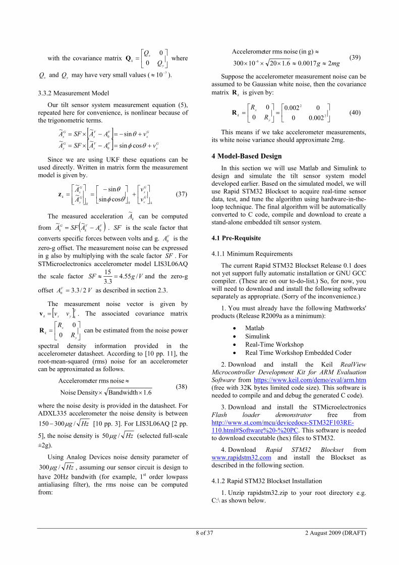
8 of 37 2 August 2009 (DRAFT)
with the covariance matrix
=
y
x
kQ
Q
0
0Q where
xQ and
yQ may have very small values ( 710−≈ ).
3.3.2 Measurement Model
Our tilt sensor system measurement equation (5), repeated here for convenience, is nonlinear because of the trigonometric terms.
[ ][ ] G
y
VV
y
G
y
G
x
VV
x
G
x
vAASFA
vAASFA
+=−×=
+−=−×=
θφ
θ
cossin~~
sin~~
0
0
Since we are using UKF these equations can be used directly. Written in matrix form the measurement model is given by.
k
G
v
G
x
kk
G
y
G
x
kv
v
A
A
+
−=
=
θφθ
cossin
sin~
~
z (37)
The measured acceleration kA~ can be computed
from ( ) ~~0
VV
k
G
kAASFA −= . SF is the scale factor that
converts specific forces between volts and g. VA0 is the
zero-g offset. The measurement noise can be expressed in g also by multiplying with the scale factor SF . For
STMicroelectronics accelerometer model LIS3L06AQ
the scale factor VgSF /55.43.3
15=≈ and the zero-g
offset VAV 2/3.30= as described in section 2.3.
The measurement noise vector is given by
[ ]Tkyxk
vv=v . The associated covariance matrix
=
y
x
kR
R
0
0R can be estimated from the noise power
spectral density information provided in the accelerometer datasheet. According to [10 pp. 11], the root-mean-squared (rms) noise for an accelerometer can be approximated as follows.
1.6BandwidthDensity Noise
noise rmster Accelerome
××
≈ (38)
where the noise desity is provided in the datasheet. For ADXL335 accelerometer the noise density is between
Hzg /300150 µ− [10 pp. 3]. For LIS3L06AQ [2 pp.
5], the noise density is Hzg /50µ (selected full-scale
±2g).
Using Analog Devices noise density parameter of
Hzg /300µ , assuming our sensor circuit is design to
have 20Hz bandwith (for example, 1st order lowpass antialiasing filter), the rms noise can be computed from:
mgg 20017.01.60210300
g)(in noise rmster Accelerome
6- ≈≈×××
≈ (39)
Suppose the accelerometer measurement noise can be assumed to be Gaussian white noise, then the covariance
matrix k
R is given by:
=
=
2
2
002.00
0002.0
0
0
y
x
kR
RR (40)
This means if we take accelerometer measurements, its white noise variance should approximate 2mg.
4 Model-Based Design
In this section we will use Matlab and Simulink to design and simulate the tilt sensor system model developed earlier. Based on the simulated model, we will use Rapid STM32 Blockset to acquire real-time sensor data, test, and tune the algorithm using hardware-in-the-loop technique. The final algorithm will be automatically converted to C code, compile and download to create a stand-alone embedded tilt sensor system.
4.1 Pre-Requisite
4.1.1 Minimum Requirements
The current Rapid STM32 Blockset Release 0.1 does not yet support fully automatic installation or GNU GCC compiler. (These are on our to-do-list.) So, for now, you will need to download and install the following software separately as appropriate. (Sorry of the inconvenience.)
1. You must already have the following Mathworks' products (Release R2009a as a minimum):
• Matlab
• Simulink
• Real-Time Workshop
• Real Time Workshop Embedded Coder
2. Download and install the Keil RealView
Microcontroller Development Kit for ARM Evaluation
Software from https://www.keil.com/demo/eval/arm.htm (free with 32K bytes limited code size). This software is needed to compile and and debug the generated C code).
3. Download and install the STMicroelectronics Flash loader demonstrator free from http://www.st.com/mcu/devicedocs-STM32F103RE-110.html#Software%20-%20PC. This software is needed to download executable (hex) files to STM32.
4. Download Rapid STM32 Blockset from www.rapidstm32.com and install the Blockset as described in the following section.
4.1.2 Rapid STM32 Blockset Installation
1. Unzip rapidstm32.zip to your root directory e.g. C:\ as shown below.

9 of 37 2 August 2009 (DRAFT)
2. Launch Matlab by double clicking the Matlab icon.
3. Click the Browser for folder button.
4. From the Browser For Folder window, select the rapidstm32\rapidstm32 subdirectory as the current working directory then click OK.
5. Run setup by typing rapidstm32_setup in the Matlab Command Window and then press ENTER on the keyboard.
6. After a successful installation, a notification will be displayed as shown below.

10 of 37 2 August 2009 (DRAFT)
4.1.3 Simulink Basics
In this step we change the current working directory to your desired directory, create a new Simulink model, and save the model.
1. Launch Matlab and click the Browse for folder button.
2. When the Browse For Folder window opens, change or create a new working directory as desire.
3. Select File/New/Model to create a new Simulink model.
4. A new Simulink model window is created.
5. Select File/Save As to save the new model.
6. Enter the new file name as tilt_system.mdl and click Save.
11 of 37 2 August 2009 (DRAFT)
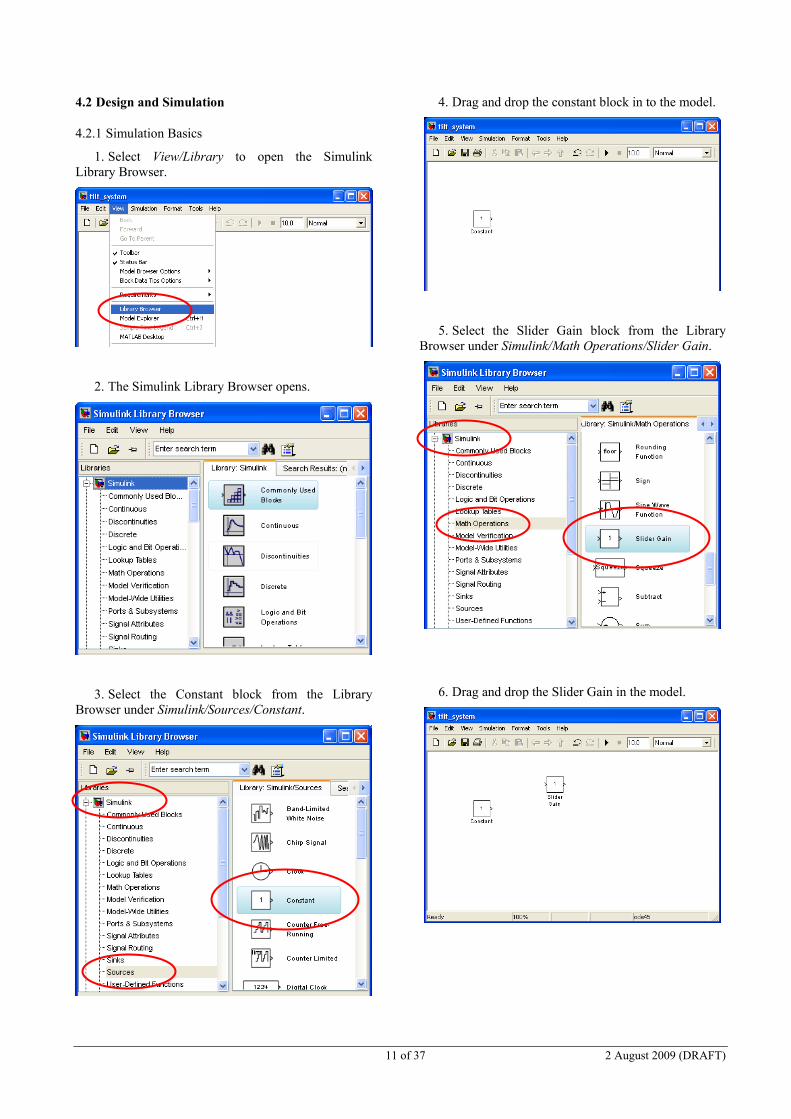
4.2 Design and Simulation
4.2.1 Simulation Basics
1. Select View/Library to open the Simulink Library Browser.
2. The Simulink Library Browser opens.
3. Select the Constant block from the Library Browser under Simulink/Sources/Constant.
4. Drag and drop the constant block in to the model.
5. Select the Slider Gain block from the Library Browser under Simulink/Math Operations/Slider Gain.
6. Drag and drop the Slider Gain in the model.

12 of 37 2 August 2009 (DRAFT)
7. Insert another Slider Gain Block in the model by “copying”. Click on the Slider Gain block in the model with the right mouse button. While still holding down the right mouse button, drag and drop another Slider Gain block in the model.
8. Rename the top Slider Gain block to “Roll (deg)” and the bottom block to “Pitch (deg)” by clicking on the name and edit it.
9. The renamed blocks.
10. Insert 2 Display blocks in the model (from the Library Browser Simulink/Sinks/Scope).
11. The inserted display blocks.
12. Change the Slider Gain block parameters by double clicking on the Slider Gain block.
Copy a block by dragging and dropping using the right
mouse button
Click on the name and edit it.

13 of 37 2 August 2009 (DRAFT)
13. Change the Roll (deg) block parameters as follows (Low – 180, High + 180). Then click Close.
14. Change the Pitch (deg) block parameters as follows (Low – 90, High + 90). Then click Close.
15. Connect blocks by dragging the signal line from the output of one block to the input of another block. The cursor changes shape to a double cross when block can be connected.
16. Completely connected Constant and Roll (deg) blocks.
17. To connect the output of the Constant block to the Pitch (deg) block input, use the right mouse button
to click on the signal line, hold the button, and drag the signal line to the input of the Pitch (deg) block.
18. The Constant block and Slider Gain blocks completely connected.
19. It is possible to re-arrange the signal line by clicking on the signal line with the left mouse button and drag it to the desired location.
Right click, hold, and drag the signal line.
Double cross.

14 of 37 2 August 2009 (DRAFT)
20. Connect all the blocks together as shown below.
21. Click the play button to run a simulation. You will notice:
• The simulation is non real-time. It runs as
fast as possible. The final time is determined in the Final simulation time edit box, in this example, 10 seconds.
• The roll and pitch angles are displayed in the Display blocks.
22. You can change the roll or pitch angle by changing the gain of the Slider Gain block to any values between the Low and High limits. Try running the simulation again by clicking the play button.
23. You can resize a block by clicking on it and drag the corner of the block to the required size.
24. To add a signal name, double click on the signal line and enter the name of the signal. Name the appropriate signal lines “roll” and “pitch”.
Resize the block by dragging
the corner of a block.
Final simulation time
Play button

15 of 37 2 August 2009 (DRAFT)
25. Add a Scope block to the model from Simulink Library Browser / Simulink / Sinks / Scope.
26. Connect the roll signal to the Scope block. (Use right mouse button to click, drag, and connect the signal line.)
27. Try changing the input type from Constant to Sinusoidal Input. Replace the Constant block in the model with a Sine Wave block (Delete the Constant block and insert a Sine Wave block from Simulink Library Browser / Simulink / Sources / Sine Wave).
28. Double click the Sine Wave block. The parameter configuration block appears. Change the Amplitude to 20 and Sample time to 0. Click OK. This will make the Sine Wave block output sine waveform with amplitude 20 unit and period 1 rad/sec.
Input Type Sine Wave

16 of 37 2 August 2009 (DRAFT)
29. Change the gain of the Slider Gain block to 1 then click Close.
30. Click Simulation/Configuration Parameters.
31. Configuration parameters dialog appears. You can configure how Simulink simulates the model:
• Time step type: Fixed or Variable.
• Solver: Discrete or ODE solver.
• Step size in seconds.
32. Set the simulation parameters as follows then click OK.
• Type: Fixed-step.
• Solver: Discrete (no continuous states).
• Fixed-step size (fundamental sample time): 0.01.
33. Try running the simulation again by clicking the play button. After the simulation is completed open the Scope block by double clicking on it. Notice that the simulation still runs in non real-time (as fast as possible).
34. Click the Binocular button to view the whole recorded data.
View all
Scope
Property
Zoom XY
Solver
Fixed-step size Type

17 of 37 2 August 2009 (DRAFT)
35. Using Scope Property. You can change how the data is displayed and logged by changing the scope parameters.
36. Zoom in the Scope using the XY magnifying glass. You will notice that the sine waveform appears continuous. This is because we set the sample time of the Sine Wave block to 0 (continuous time).
37. Simulink simulation works by solving block algebra and using the built-in differential equation solver. Sample time step used by the numerical integration algorithm is determined based on either the block’s sample time parameters or the solver fundamental sample time. You can see the sample time that each block operates simply by selecting Format/Sample Time Display/Colors.
38. The Sample Time Legend appears. The blocks’ color also change according to the block’s sample time. The Scope and the two Display blocks (Display and Display1) are in red (Discrete sample time 0.01 sec) because we set the simulation configuration parameter to 0.01 sec earlier on. The Sine Wave block is black (continuous-time) because we set the sample time of the Sine Wave block to 0 (continuous). The Slider Gain blocks are continuous-time because they inherit sample time from the Sine Wave block.
Plot more than
one signal
Determine how much data to
record
Zoom XY

18 of 37 2 August 2009 (DRAFT)
39. Double click on the Sine Wave block and change the sample time to 0.01 sec.
40. Run the simulation again and double click the Scope block to see the output sine waveform. You will notice that all blocks’ color change to red. Now, all blocks’ sample time is 0.01.
41. The output sine waveform clearly illustrates discrete-time step of 0.01 sec.
42. To make simulation run in real-time, insert a real-time block in the model. Insert a Real-Time Block in the model from Simulink Library Browser / Rapid STM32 Blockset / Add-on Modules / Real-Time Block).
Inserted Real-Time Block
Zoomed-in
0.01 sec

19 of 37 2 August 2009 (DRAFT)
43. Click “Update diagram” button twice or until the Real-Time Block displays a correct sample time.
44. Run the simulation again by clicking the play button. Now the model update in real-time using time step 0.01 sec.
45. It is possible to adjust the tilt angle and see changes in the output in real-time.
• Make simulation run indefinitely by changing final simulation time to “inf”.
• Replace the Sine Wave block with a Constant block.
• Double click the Slider Gain block to open the slider.
• Run the simulation.
4.2.2 Sensor Model
We will implement a very simple discrete-time accelerometer model in Simulink. Substitute
( ) ~~0
VV
k
G
kAASFA −= in the measurement equation (37)
yields.
( )( ) G
v
VV
y
G
y
G
x
VV
x
G
x
vAASFA
vAASFA
+=−=
+−=−=
θφ
θ
cossin~~
sin~~
0
0 (41)
Hence
( )
( ) VG
y
V
y
VG
x
V
x
AvSF
A
AvSF
A
0
0
cossin1~
sin1~
++=
++−=
θφ
θ (42)
The followings describe how to implement (42) using Simulink.
1. Insert a gain block into the model from Simulink Library Browser / Simulink / Math Operations / Gain.
2. Double click on the Gain block. Set the value of gain to pi/180. Leave the Sample time as -1 to inherit the sample time of input signal. Rename the block “D2R”.
Update diagram button
Real-Time Block displays the correct
sample time of 0.01 sec.
The Scope updates
in real-time.
Simulation time updates in real-
time.
Constant block
Adjust slider gain.
See changes in output
Scope in real-time.
Use “inf” as final simulation time.

20 of 37 2 August 2009 (DRAFT)
3. Make another copy of the D2R block in the model. If you can not see the gain value, enlarge the block to a bigger size.
4. Insert a Trigonometric Function block in the model from Simulink Library Browser / Simulink / Math Operations / Trigonometric Function.
5. Insert two more Trigonometric Function blocks, one as a sin another as a Cos block. Double click on the Trigonometric Function block to open the configuration parameters dialog and change its parameters appropriately.
pi/180 convert from
degree to radians
sin
sin
cos

21 of 37 2 August 2009 (DRAFT)
6. Insert a Product block in the model from Simulink Library Browser / Simulink / Math
Operations / Product.
7. Insert 3 more gain blocks. One block with the gain value of -1. Two blocks with the values of 3.3/15. Rename the last 2 blocks “SF g2V” to represent a scale factor that convert measurement from g to volts.
8. Insert two Sum blocks in the model from Simulink Library Browser/Simulink/Math Operations/Sum.
9. Double click on the top Sum block and change its setting to ++|.
10. The input port location of the top Sum block change as follows.
3.3/15
-1
3.3/15

22 of 37 2 August 2009 (DRAFT)
11. Insert 2 Band-Limited White Noise in the model from Simulink Library Browser/Simulink/ Sources/Band-Limited White Noise.
12. Set the following parameters to both Band-Limited White Noise blocks.
• Set “Sample time” to 0.01 will set the block’s sample time to 0.01 seconds.
• Set the “Noise power” to Noise Variance times
Sample time i.e. 01.0002.0 2 × will set the
output noise variance to (2mg)2.
• Change the “Seed” to any random number so that the two blocks have different seeds.
13. Insert two more Sum blocks and a Constant block. Rename the Constant block “zero-g offset”. Set the zero-g offset constant value to 3.3/2.
14. Connect all blocks together as shown below.
The Seed is used to initialize random number generator. Different seeds ensure that the block generates different
noise sequence.

23 of 37 2 August 2009 (DRAFT)
15. Select all blocks by dragging the cursor to include all blocks just created.
16. Click the right mouse button while the cursor is on one of the selected blocks. Select “Create Subsystem”
17. A new subsystem is created. Rename it “Accelerometer Sensor”.
18. Double click the newly created subsystem block and rename the input and output port as follows.
• In1 to Roll (deg)
• In2 to Pitch (deg)
• Out1 to Ay (V)
• Out2 to Ax (V)
19. The renamed port names appears on the subsystem block.
20. Double click the subsystem to open it. Double click the Ax (V) port block and change its Port number property to 1. Ax (V) now will appear on the top.
Output
port
Input port

24 of 37 2 August 2009 (DRAFT)
21. Close the subsystem block. Connect the roll and pitch signal to Roll (deg) and Pitch (deg) input port respectively.
22. Insert a Scope block in the model from Simulink Library Browser/Simulink/Sinks/Scope.
23. Double click the Scope block to open it. Click the Scope Property button. Change the “Number of axes” property to 2.
24. The Scope now has 2 input ports. Connect the Ax (V) and Ay (V) output ports to the top and bottom Scope In port respectively. Name the signal Ax_V and Ay_V as shown below.
25. Click Update Diagram (or Ctrl-D) until the Real-
Time block displays a correct model sample time, in our case 0.01 sec. Ensure that:
• The final simulation time is “inf”.
• The Real-Time block displays a correct model simulation time. (A model simulation time is the base time step or the smallest time step in the model.)

25 of 37 2 August 2009 (DRAFT)
26. Run the model. Notice that, with the inclusion of the Real-Time block, the simulation runs in real-time. The output of the Accelerometer Sensor subsystem is the noisy output in volts (Ax_V and Ay_V) that we expect to get from real accelerometers. During the simulation you can change the Slider Gain of either the roll or pitch angle, changes in output voltages can be seen simultaneously in the Scope.
4.2.3 UKF Algorithm
In this section we implement and simulate the UKF for tilt sensor system. You will see that implementing UKF is simplified considerably using Embedded Matlab Function block because your algorithm can be programmed in M-Script.
The discrete-time system model for UKF is based on equations (33) and (37) which is repeated here for convenience.
Process model
ky
x
kkw
w
+
=
+θφ
θφ
10
01
1
Measurement model
k
G
v
G
x
kk
G
y
G
x
kv
v
A
A
+
−=
=
θφθ
cossin
sin~
~
z
1. Insert a Quantizer block in the model and rename them ADC (from Simulink Library Browser / Simulink / Discontinuities / Quantizer. In this model we will use a Quantizer block as our simplified model of Analog to Digital Converter (ADC) found in most microcontrollers.
Changes in Ay_V when roll angle
changes.

26 of 37 2 August 2009 (DRAFT)
2. Double click the ADC block. The Quantizer ‘s Function Block Parameters opens. Insert 3.3/2^12 in the Quantization interval edit box. This is our simplified model of a single-end 12-bits ADC having 3.3 V supply voltage. Leave the Sample time -1 to inherit sample time from input signal.
3. Insert a Mux block in the model from Simulink Library Browser / Simulink / Signal Routing.
4. Insert an Embedded Matlab Function block in the model from Simulink Library Browser/Simulink/User-Defined Functions/Embedded MATLAB Function.
5. Insert a Constant block in the model. Rename this block “x0”. Double click the Constant block and insert [0;0] in the Constant value edit box. This block is the
initial state estimates 0
x for UKF.
6. Insert a Constant block in the model. Rename this block “P0”. Double click the Constant block and insert ([10 0;0 10]*pi/180).^2 in the Constant value edit box. This block is the initial state estimates error covariance
matrix 0
P for UKF. This is saying that the standard
deviation of the estimation error is 10 degrees.

27 of 37 2 August 2009 (DRAFT)
7. Insert two Gain blocks (from Simulink Library Browser / Simulink / Math Operations / Gain). Rename them “R2D”. These blocks are used to convert from radians to degrees. Input 180/pi in the Gain edit box.
8. Insert 2 Demux block in the model from Simulink Library Browser/Simulink/Signal Routing/ Demux.
9. Insert 2 Mux blocks in the model (from Simulink Library Browser/Simulink/Signal Routing/Mux).
10. Insert 2 Goto and 2 From blocks in the model (from Simulink Library Browser/Simulink/Signal
Routing/ Goto or From).
11. Insert 2 Scope blocks in the model (from Simulink Library Browser / Simulink / Sinks / Scope).
12. Double click the Goto and From block and edit the Goto Tag to “TrueRoll” and “True Pitch”.

28 of 37 2 August 2009 (DRAFT)
After the Goto and From blocks have been modified, the model should appear as shown above.
13. Rename the Embedded MATLAB Function block to “UKF”. Double click the block. An editor opens.
14. Delete the existing code. Copy and paste the source code in Appendix A in to the Embedded MATLAB Editor, Save and Close the Editor.
15. The input and output ports of the UKF block should now change to reflex the input and output parameters of the “tilt_sensor_ukf” function.

29 of 37 2 August 2009 (DRAFT)
16. Route the signals and the final model as shown above.
17. Run the simulation. Sample state estimation and associated standard deviation is shown below.
4.2.4 UKF Performance Analysis
In this section we will analyze performances of the UKF. In practice, when a Kalman filter is used to estimate system states, it also provides information about the accurate of the estimates. This information is embedded in the error covariance matrix P .
The simplest method to analyze performances of a Kalman filter, under simulation environment, is by comparing the computed error covariance P with actual errors. The process is as follows.
• Derive the theoretical estimation error standard deviation by taking the squared root of the diagonal
terms of the matrix +P .
• Derive the actual estimation errors by finding differences between actual states and state estimates.
• Compare the two.
• It should be noted that the theoretical estimation error standard deviation derived from P is computed based on actual state estimates. Therefore, to be perfect, you should collect data from several random runs (known as Monte Carlo simulation) and compare the averaged values.
An example of error covariance analysis proceeds as follows.
30 of 37 2 August 2009 (DRAFT)
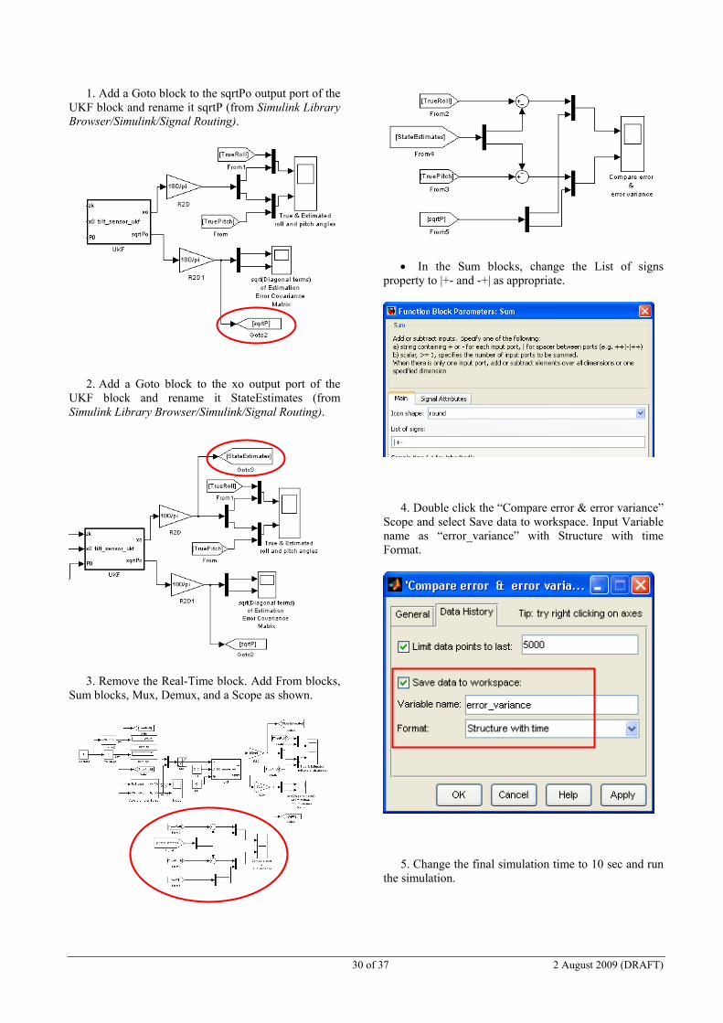
1. Add a Goto block to the sqrtPo output port of the UKF block and rename it sqrtP (from Simulink Library Browser/Simulink/Signal Routing).
2. Add a Goto block to the xo output port of the UKF block and rename it StateEstimates (from Simulink Library Browser/Simulink/Signal Routing).
3. Remove the Real-Time block. Add From blocks, Sum blocks, Mux, Demux, and a Scope as shown.
• In the Sum blocks, change the List of signs property to |+- and -+| as appropriate.
4. Double click the “Compare error & error variance” Scope and select Save data to workspace. Input Variable name as “error_variance” with Structure with time Format.
5. Change the final simulation time to 10 sec and run the simulation.

31 of 37 2 August 2009 (DRAFT)
6. Results from a single simulation run in the “Compare error & error variance” Scope are shown below. The yellow lines are the actual errors while the purple lines are the theoretical error standard deviation
(the squared-root values of the diagonal terms of +P ).
In theory, 63% of the actual errors should lie inside the 1 standard deviation bound.
7. Run the Matlab code in Appendix B in the Matlab Command Window to plot and compute the actual error standard deviation and compare with the theoretical values. Both values should be close to each other.
8. Change the seed value of the Band-Limited White Noise blocks to seed1 and seed2 as shown below.

32 of 37 2 August 2009 (DRAFT)
9. Run the Matlab code in Appendix C in the Matlab Command Window. This code simulates the tilt_system Simulink model for 100 runs automatically using different noise seeds (Monte Carlo technique). The simulation results are shown below. The actual mean and standard deviation errors should be as close
to zero and Diagonal
P as possible respectively, to
indicate correct filter operations. If the mean or the standard deviation of errors differ significantly from these conditions, a “filter Diverge” is said to occur where corrective actions must be taken.
5 References
1. Siouris, G. M., “Aerospace Avionics Systems: A Modern Synthesis”, 1st ed., Academic Press, Inc., 1993, pp. 20-22.
2. STMicroelectronics, LIS3L06AL MEMS INERTIAL SENSOR: 3-axis - +/-2g/6g ultracompact linear accelerometer datasheet, May 2006. pp.5.
3. Kalman, R.E. 1960. A new approach to linear filtering and prediction problems, Transaction of the ASME, Journal of Basic Engineering: 35-45
4. Leonard, A. McGee and Stanley F. Schmidt. November 1985. Discovery of the Kalman Filter as a practical tool for aerospace and industry, NASA Technical Memorandum 86847
5. Sorenson, Harold. W. 1985. Kalman Filtering: Theory and Applications. IEEE Press
6. Brown, R. G. and Hwang, Y. C., “Introduction to random signals and applied Kalman filtering”, John Wiley & Sons, 1997, pp.214-20.
7. Julier, S. J. and Uhlmann, J. K., A New Extension of the Kalman Filter to Nonlinear Systems, http://www.cs.unc.edu/~welch/kalman/media/pdf/Julier1997_SPIE_KF.pdf, 2009.
8. Julier, S. J. and Uhlmann, J. K., Unscented Filtering and Nonlinear Estimation, Proceedings of The IEEE, Vol. 92, No. 3, March 2004., http://citeseerx.ist .psu.edu/viewdoc/download?doi=10.1.1.136.6539&rep=rep1&type=pdf
9. Simon, D., “Optimal State Estimation”, Wiley-Interscience, 2006., pp. 448-51.
10. Analog Devices, Accelerometer ADXL335 Datasheet, Rev.0., 2009.
33 of 37 2 August 2009 (DRAFT)
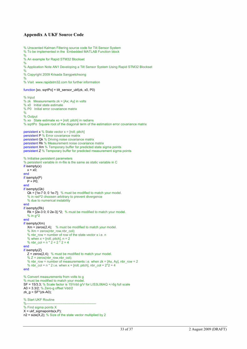
Appendix A UKF Source Code
% Unscented Kalman Filtering source code for Tilt Sensor System % To be implemented in the Embedded MATLAB Function block % % An example for Rapid STM32 Blockset % % Application Note AN1 Developing a Tilt Sensor System Using Rapid STM32 Blockset % % Copyright 2009 Krisada Sangpetchsong % % Visit www.rapidstm32.com for further information function [xo, sqrtPo] = tilt_sensor_ukf(zk, x0, P0) % Input % zk Measurements zk = [Ax; Ay] in volts % x0 Initial state estimate % P0 Initial error covariance matrix % % Output % xo State estimate xo = [roll; pitch] in radians % sqrtPo Square root of the diagonal term of the estimation error covariance matrix persistent x % State vector x = [roll; pitch] persistent P % Error covariance matrix persistent Qk % Driving noise covariance matrix persistent Rk % Measurement noise covariance matrix persistent Xm % Temporary buffer for predicted state sigma points persistent Z % Temporary buffer for predicted measurement sigma points % Initialise persistent parameters % persistent variable in m-file is the same as static variable in C if isempty(x) x = x0; end if isempty(P) P = P0; end if isempty(Qk) Qk = [1e-7 0; 0 1e-7]; % must be modified to match your model. % in rad^2 choosen arbitrary to prevent divergence % due to numerical instability end if isempty(Rk) Rk = [2e-3 0; 0 2e-3].^2; % must be modified to match your model. % in g^2 end if isempty(Xm) Xm = zeros(2,4); % must be modified to match your model. % Xm = zeros(nbr_row,nbr_col); % nbr_row = number of row of the state vector x i.e. n % when x = [roll; pitch], n = 2 % nbr_col = n * 2 = 2 * 2 = 4 end if isempty(Z) Z = zeros(2,4); % must be modified to match your model. % Z = zeros(nbr_row,nbr_col); % nbr_row = number of measurements i.e. when zk = [Ax, Ay], nbr_row = 2 % nbr_col = n * 2 i.e. when x = [roll; pitch], nbr_col = 2*2 = 4 end % Convert measurements from volts to g % must be modified to match your model. SF = 15/3.3; % Scale factor is 15/Vdd g/V for LIS3L06AQ +/-6g full scale A0 = 3.3/2; % Zero-g offset Vdd/2 zk_g = SF*(zk-A0); % Start UKF Routine %--------------------------------------------------------------- % Find sigma points X X = ukf_sigmapoints(x,P); n2 = size(X,2); % Size of the state vector multiplied by 2

34 of 37 2 August 2009 (DRAFT)
% Predicted states for next time step computed from the sigma points X for k = 1:n2 Xm(:,k) = updatex(X(:,k)); end % Find the prediction mean and covariance matrix [xm, Pm] = ukf_mean_covariance(Xm); Pm = Pm + Qk; % Predicted measurements sigma points for k = 1:n2 Z(:,k) = h(Xm(:,k)); % must be modified to match your model (only if the h function has more input or output parameters). end % Find mean and covariance [z, Pz] = ukf_mean_covariance(Z); Pz = Pz + Rk; Pxz = ukf_covariance(Xm, Z); % Cross covariance matrix Kk = Pxz/Pz; % Kalman gain matrix x = xm + Kk*(zk_g - z); % Find the state estimates P = Pm - Kk*Pz*Kk'; % Estimation error covariance matrix P = 0.5*(P+P'); % Prevent numerical problem xo = x; sqrtPo = sqrt(diag(P)); % end tilt_sensor_ukf %-------------------------------------------------- % This is the nonlinear measurement model % This function h(x) must be modified to match your measurement model. function z = h(x) z1 = -sin(x(2)); z2 = sin(x(1))*cos(x(2)); z = [z1; z2]; %-------------------------------------------------- % This function is used to propagate the state vector % from time step tk to tk+1. % In our tilt sensor system the propagation is quite simple % since we are estimating constants. % This function updatex (x) must be modified to match your process model. function xo = updatex(x) % From F = [0 0; 0 0] % expm(F) = [1 0; 0 1]; % i.e. xo(1) = x(1), xo(2) = x(2), ... xo = x; % If the process model is highly nonlinear, % it is possible to use more accurate numerical integration techniques % such as 4th order Runge Kutta method to propagate the states. % % Example: 4th order Runge Kutta Update Routine % function xo = updatex_RungeKutta(x, dt, varin) % % varin is the input arguments % dt is the sample time (tk+1 - tk) % % h_by2 = 0.5*dt; % k1 = fx(x, varin); % k2 = fx(x + k1*h_by2, varin); % k3 = fx(x + k2*h_by2, varin); % k4 = fx(x + k3*h, varin); % xo = x + (h/6)*(k1 +2*(k2 + k3) + k4); % % where the nonlinear differential equations are defined as follows. % % function dx = fx(x, varin) % % dx1 = f1(x,varin);

35 of 37 2 August 2009 (DRAFT)
% dx2 = f2(x,varin); % ... % dx = [dx1; dx2; ...] %%%%%%%%%%%%%%%%%%%%%%%%%%%%%%%%%%%%%%%%%%%%%%%%%%% % It is not necessary to modify the following three functions AT ALL. % function X = ukf_sigmapoints(xbar,Pi) % function [m, P] = ukf_mean_covariance(sigmaX) % function P = ukf_covariance(sigmaX, sigmaY) % These functions can be used in any UKF systems. %%%%%%%%%%%%%%%%%%%%%%%%%%%%%%%%%%%%%%%%%%%%%%%%%%% %-------------------------------------------------- % This function is used to compute the sigma points % Input % xbar is the mean value of x % Pi is the associated covariance matrix % % Output % X is the sigma points % The size of X is determined as follows. % The number of rows is the same as the number of rows of xbar i.e. n % The number of columns is 2*n % Optimal state estimation, Dan Simon, p. 446 ISBN 100471708585 function X = ukf_sigmapoints(xbar,Pi) n = size(xbar,1); A = chol(n*Pi)'; % R = chol(A) where R'*R = A X = [A -A] + repmat(xbar,1,n*2); %-------------------------------------------------- % This function computes the mean and covariance matrix from the sigma points. % m is the mean computed from the sigma points. % P is the covariance matrix computed from the sigma points and the mean. function [m, P] = ukf_mean_covariance(sigmaX) n2 = size(sigmaX,2); m = sum(sigmaX,2)/n2; P = zeros(size(sigmaX,1)); % size n for k = 1:n2 P = P + ((sigmaX(:,k)-m)*(sigmaX(:,k)-m)'); end P = P/n2; %-------------------------------------------------- % This function computes the cross covariance matrix from two sets of sigma points. % P is the cross covariance matrix computed from the sigma points and the mean. % sigmaX and sigmaY are the sigma points of X and Y respectively. function P = ukf_covariance(sigmaX, sigmaY) n2 = size(sigmaX,2); % 2*n mx = sum(sigmaX,2)/n2; my = sum(sigmaY,2)/n2; P = zeros(size(sigmaX,1),size(sigmaY,1)); % size n for k = 1:n2 P = P + ((sigmaX(:,k)-mx)*(sigmaY(:,k)-my)'); end P = P/n2;

36 of 37 2 August 2009 (DRAFT)
Appendix B Error Variance Analysis
% Error variance analysis for 1 simulation run % % An example for Rapid STM32 Blockset % % Application Note AN1 Developing a Tilt Sensor System Using Rapid STM32 Blockset % % Copyright 2009 Krisada Sangpetchsong % % Visit www.rapidstm32.com for further information % Import data from saved work space data time = error_variance.time; true_roll_error_deg = error_variance.signals(1).values(:,1); theoretical_roll_error_deg = error_variance.signals(1).values(:,2); true_pitch_error_deg = error_variance.signals(2).values(:,1); theoretical_pitch_error_deg = error_variance.signals(2).values(:,2); % Compute actual error standard deviation actual_roll_std_deg = std(true_roll_error_deg) actual_pitch_std_deg = std(true_pitch_error_deg) % Plot results subplot(2,1,1) plot(time,true_roll_error_deg,'r-',time,theoretical_roll_error_deg,'b-',time,... -theoretical_roll_error_deg,'b-') ylabel('Roll Errors (deg)'), xlabel('time (sec)') legend('Actual errors','\surd(P_{11})') text(0.05,0.2,['Actual roll error std = ' num2str(actual_roll_std_deg) 'deg'],'unit','normalized') subplot(2,1,2) plot(time,true_pitch_error_deg,'r-',time,theoretical_pitch_error_deg,'b-',time,... -theoretical_pitch_error_deg,'b-') ylabel('Pitch Errors (deg)'), xlabel('time (sec)') legend('Actual errors','\surd(P_{22})') text(0.05,0.2,['Actual pitch error std = ' num2str(actual_pitch_std_deg) 'deg'],'unit','normalized')

37 of 37 2 August 2009 (DRAFT)
Appendix C Monte Carlo Simulation
% Error variance analysis for 100 simulation runs (Monte Carlo) % % An example for Rapid STM32 Blockset % % Application Note AN1 Developing a Tilt Sensor System Using Rapid STM32 Blockset % % Copyright 2009 Krisada Sangpetchsong % % Visit www.rapidstm32.com for further information clc % clear screen start = 0; % sec stop = 10; % sec final_run = 100; % Number runs to simulate % Generate random seeds to drive the Band-Limited White Noise Block in % the Accelerometer Sensor Subsystem % the seed is picked from a uniform random variable between begin_bound and % end_bound RandStream.setDefaultStream(RandStream('mt19937ar','seed',sum(100*clock))); % set random seed based on clock begin_bound = 0; end_bound = 10000; seed_vec = floor(begin_bound + (end_bound - begin_bound).*rand(2,final_run)); for k = 1:final_run seed1 = seed_vec(1,k); seed2 = seed_vec(2,k); disp(['Run' num2str(k)]) sim('tilt_system',[start stop]); % This line of code starts and stops Simulink simulation automatically. if (k == 1) % First run % initialise record buffer true_roll_error_deg_rec = repmat(error_variance.signals(1).values(:,1),1,final_run); theoretical_roll_error_deg_rec = repmat(error_variance.signals(1).values(:,2),1,final_run); true_pitch_error_deg_rec = repmat(error_variance.signals(2).values(:,1),1,final_run); theoretical_pitch_error_deg_rec = repmat(error_variance.signals(2).values(:,2),1,final_run); else % Other runs % Import data from saved work space data true_roll_error_deg_rec(:,k) = error_variance.signals(1).values(:,1); theoretical_roll_error_deg_rec(:,k) = error_variance.signals(1).values(:,2); true_pitch_error_deg_rec(:,k) = error_variance.signals(2).values(:,1); theoretical_pitch_error_deg_rec(:,k) = error_variance.signals(2).values(:,2); end end time = error_variance.time; mean_true_roll_error_deg = mean(true_roll_error_deg_rec,2); mean_theoretical_roll_error_deg = mean(theoretical_roll_error_deg_rec,2); mean_true_pitch_error_deg = mean(true_pitch_error_deg_rec,2); mean_theoretical_pitch_error_deg = mean(theoretical_pitch_error_deg_rec,2); std_true_roll_error_deg = std(true_roll_error_deg_rec,0,2); std_true_pitch_error_deg = std(true_pitch_error_deg_rec,0,2); % Plot results subplot(2,1,1) plot(time,mean_true_roll_error_deg,'r-',time,mean_theoretical_roll_error_deg,'b-',time,... std_true_roll_error_deg,'g-') ylabel('Roll Errors (deg)'), xlabel('time (sec)') legend('Mean errors','\surd(P_{11})','Error std') subplot(2,1,2) plot(time,mean_true_pitch_error_deg,'r-',time,mean_theoretical_pitch_error_deg,'b-',time,... std_true_pitch_error_deg,'g-') ylabel('Pitch Errors (deg)'), xlabel('time (sec)') legend('Mean errors','\surd(P_{22})','Error std')