Embed Size (px)
Citation preview

HAL Id: tel-01127571https://tel.archives-ouvertes.fr/tel-01127571
Submitted on 7 Mar 2015
HAL is a multi-disciplinary open accessarchive for the deposit and dissemination of sci-entific research documents, whether they are pub-lished or not. The documents may come fromteaching and research institutions in France orabroad, or from public or private research centers.
L’archive ouverte pluridisciplinaire HAL, estdestinée au dépôt et à la diffusion de documentsscientifiques de niveau recherche, publiés ou non,émanant des établissements d’enseignement et derecherche français ou étrangers, des laboratoirespublics ou privés.
An upscaled study of a membrane filtration process inpresence of biofilms
Sepideh Habibi
To cite this version:Sepideh Habibi. An upscaled study of a membrane filtration process in presence of biofilms. Chemicaland Process Engineering. Ecole Centrale Paris, 2014. English. �NNT : 2014ECAP0042�. �tel-01127571�

DRAFT
THESE
POUR L’OBTENTION DU GRADE DE
DOCTEUR DE L’ECOLE CENTRALE DES ARTS ET MANUFACTURES
SPECIALITE : GENIE DES PROCEDES
Caracterisation multi-echelles d’un systeme de filtration en presense d’un biofilm
PRESENTEE PAR : SEPIDEH HABIBI
DIRECTEURS DE THESE : BENOIT GOYEAU,MOHAMMED RAKIB
ENCADRANTS : FABIEN BELLET, ESTELLE COUALLIER, FILIPA LOPES
SOUTENUE LE 08/07/2014
JURY
PATRICE BACCHIN PROFESSEUR-LGC-TOULOUSE (RAPPORTEUR)
GERALD DEBENEST PROFESSEUR-MIFT-TOULOUSE (RAPPORTEUR)
BENOIT GOYEAU PROFESSEUR-ECP (DIRECTEUR)
MOHAMMED RAKIB PROFESSEUR-ECP (DIRECTEUR)
PATRICK DI MARTINO PROFESSEUR-ERRMECE (EXAMINATEUR)
MURIELLE RABILLER-BAUDRY PROFESSEUR-UNIV-RENNES-1 (EXAMINATRICE)
FABIEN BELLET MAITRE DE CONFERENCES-ECP (CO-ENCADRANT)
ESTELLE COUALLIER CHARGEE DE RECHERCHE (CO-ENCADRANTE)
FILIPA LOPES ENSEIGNANT-CHERCHEUR-ECP (CO-ENCADRANTE)
DELIVRE PAR : ECOLE CENTRALE PARIS - ECOLE DOCTORALE 287 - SCIENCES POUR L’INGENIEUR
UNITE DE RECHERCHE : LABORATOIRE DE GENIE DES PROCEDES ET MATERIAUX - EA 4038


ACKNOWLEDGMENTS
Research activity requires a high level of planning, executing and discussing. One needs
innovative opinions, active contributions, continuous support and encouragement to elab-
orate the maximum of results . I think that a thesis project is not a personal achievement
but the result of an enriching experience involving a group of researchers. During these
last three years, I have been supported by many people to whom I am very grateful.
I would like to express my deep gratitude to my supervisor Professor Benoıt Goyeau. He
gave me great intellectual freedom to pursue my interests and provided encouragement
and guidance throughout this work’s lifetime. But, most I would like to thank him for his
moral support during the ups and downs of my thesis years.
I would also like to thank my research supervisors, Professor Mohammed Rakib, for
providing me such a good opportunity to work with him and letting me enter and enjoy
the research world.
I would like to express my sincere gratitude to my supervisor Dr. Fabien Bellet, who gave
me a lot of his time, pushed my limits constantly with his encouragement and supported
me with positive energy. During the past three years, he not only helped me with my
research project, but also cared for difficult moments I have been through both in personal
and professional levels.
Special thank to my supervisor Dr. Filipa Lopes, for her guidance, valuable scientific
participation and useful critics of this research work.
I would also like to thank deeply my supervisor Dr. Estelle Couallier, for her contribution
in this research project and for her continuous encouragement and helpful discussions
during these years. I would also like to extend my thanks to the jury members; reviewers
and invited professors. First I would like to send my gratitude to Pr. Patrice Bacchin,
Pr. Geerard Debenest for accepting to review my thesis. Then, I would especially like to
thank Pr. Murielle Rabiller-Baudry for both for accepting to review this work and also for
teaching me the FTIR-ATR technique. I truly appreciated her moral support during our
collaboration in Rennes. I would also like to thank Pr. Patrick Di Martino for accepting to
participate as an invited member and for his eventual remarks. Last and not least, I would
like to thank Pr. Francisco Valdes-Parada for his assistance in developing the biofilm
model, but most for being humble and so friendly.
ECOLE CENTRALE PARIS i

My special thanks are extended to the Laboratory staff Nathalie, Barbara, Helene, Vin-
cent, Cyril and Thierry for their help in offering me the resources in running my experi-
ments and in treating the results.
And of course, I would like to thank my office colleagues that changed every now and
then, but even so we managed to create a special bound that I wish last with time. So,
special thanks to Barbara, Quentin, Carmen and Zhaohuan who already left the laboratory
while ago. Best wishes for Pascal on his research projects, and a special thank to Nadine
for her continuous encouragement and support.
A special thank to my family. Words cannot express how grateful I am to my mother and
father for all the sacrifices that they made so that I can achieve my dreams. The distance
separated us for so long but you were always with me, making me stronger. Special
thanks to my sister for her special support and patience. And last but not least, special
thanks to my boyfriend for his love and support. Without them, I can not overcome any
difficulties.

RESUME
Dans un procede de filtration, un fluide traverse une membrane (barriere selective). Une
force motrice s’applique entre les deux cotes de la membrane qui peut etre un gradi-
ent de pression, temperature ou un potentiel electrique/chimique. Dans les procedes de
filtration par un gradient de pression, certains composes du milieu fluide, traversent la
membrane alors que d’autres sont retenues sur la surface membranaire. Ces procedes
sont tres utiles dans differents domaines de l’industrie, notamment en ce qui concerne le
traitement des eaux et des effluents, biotechnologie, agroalimentaire et pharmacie. En
plus les procedes de filtration offrent des installations plus compactes avec une optimi-
sation des couts operationnels comparant avec des procedes traditionnels de separation
notamment distillation et cristallisation. Par ailleurs, ces procedes se realisent en absence
des additifs chimique et changement de la phase. Dans cette etude, on se focalise sur les
procedes de microfiltration.
L’inconvenient principal de ces procedes est l’accumulation continue de partic-
ules/molecules sur la surface de la membrane. Ceci affecte la selectivite de la membrane,
modifie la qualite et la quantite de liquide passant a travers la membrane et conduit a
une augmentation des couts et de l’energie. Le Colmatage (encrassement) membranaire
se produit dans tous les types de procedes membranaires et par consequent est connu le
principal obstacle a l’utilisation repandue de ces procedes.
Differentes techniques sont utile pour surmonter les effets de l’encrassement de la per-
formance de la membrane: le traitement physico-chimique des membranes utilisees, la
modification des conditions operatoires (flux tangentiel de la solution d’alimentation sur
la surface de la membrane est souvent applique pour reduire au minimum l’accumulation
de particules), l’utilisation de membranes moins sensibles au colmatage, etc.
Tout dependant de la nature des solutions traitees, les particules deposees sont tres
variables. Les micro-organismes, des matieres organiques naturelles notamment les
proteines, les polysaccharides, les substances humides, les oxydes inorganiques et les
sels contribuent au colmatage des membranes.
Dans les dernieres annees, un grand nombre d’etudes experimentales ont ete investis
pour comprendre les mecanismes de colmatage. Il a ete souligne que les proprietes
physico-chimiques de la membrane, la chimie des solutions et les conditions operatoires
sont les trois principaux facteurs influant sur les mecanismes de colmatage. En par-
ECOLE CENTRALE PARIS iii

allele, les modeles theoriques ont ete proposes pour confirmer / decrire les observations
experimentales.
La modelisation du colmatage membranaire est un outil essentiel pour evaluer les
mecanismes qui le causent. Il permet egalement predire la performance du systeme de
filtration et par consequent trouver des strategies adaptees pour empecher la modification
de la performance membranaire pendant le procede de filtration.
En general, les modeles de classifient en deux grandes categories: les modeles de
transport de masse qui se concentrent sur la transport de solutes dans le procede de fil-
tration, et les modeles de colmatage bases sur le blocage des particules/molecules sur la
surface ou a lnterieur de la membrane. Dans la plupart des cas, les modeles dependent
fortement des parametres empiriques ou semi-empiriques et restent phenomenologique.
Deux objectifs principaux ont ete fixes pour le travail present:
1. Avoir une meilleure comprehension des mecanismes du colmatage membranaire
lors de la filtration d’un milieu liquide contenant les micro-organismes en suspen-
sion. Il est important de souligner que des eaux industrielles et des eaux usees dans
plusieurs domaines appartiennent a ce type d’effluents.
2. Proposer un modele macroscopique decrivant les mecanismes de colmatage ob-
serves.
Au cours de la filtration de ce type de solution, d’une part, les bacteries se deposent a
la surface de la membrane et developpent progressivement un film biologique (biofilm)
et d’autre part les matieres organiques naturelles secretees par le biofilm sccumulent sur
la surface de la membrane et adsorbent partiellement ou bloquent les pores interieurs.
Il est interessant de noter que le colmatage membranaire issue des matieres organiques
naturelles (telles que les proteines, les polysaccharides, les substances humides), est elle-
meme un phenomene complexe impliquant la formation d’un gradient de concentration a
proximite de la surface de la membrane (la polarisation de concentration) et d’une serie
de mecanismes (formation d’un gteau, adsorption, blocage des pore).
durant le procede de filtration, la resistance initiale de la membrane augmente non
seulement par la resistance supplementaire du biofilm; mais aussi par la penetration et
l’adsorption / depot de composes secretes (de biofilm) sur les pores de la membrane
interne. En conclusion, les deux mecanismes simultanes (formation de biofilm a la
surface de la membrane et le colmatage membranaire en volume) meritent d’etre etudiees
separement afin d’obtenir une description plus precise des phenomenes mis en jeu dans
chacun d’eux.
Les structures des biofilm et membrane sont tres complexes et heterogenes dans l’espace
et le temps. Ils peuvent etre consideres comme des milieux poreux multi-echelle. En
fait, plusieurs longueurs caracteristiques sont presentes a l’echelle du pore: des composes
chimiques comme des proteines (quelques nanometres), les bacteries (1-2 µm) et les pores
de la membrane (cent nanometres). En outre, l’epaisseur du biofilm et la membrane varie
entre quelques µm jusqu’a des centaines de µm. Il ne faut pas oublier que le temps

caracteristique des phenomenes de transport (convection, diffusion, adsorption, reaction
cellulaire) est tres variable egalement. Il convient de souligner que l’heterogeneite du
biofilm et la membrane rend l’approche de la modelisation difficile.
En raison de la complexite du probleme du colmatage membranaire, deux systemes
(membrane et biofilm) sont etudiees et modelisees separement dans ce travail.
Tout d’abord l’adsorption des proteines a la surface de la membrane est etudiee
experimentalement et theoriquement. On rappelle que les proteines ne sont pas les
seules especes produites par le biofilm, cependant, dans ce travail, ils representent le
produit extracellulaire du biofilm pour simplifier les complexites. En suite, l’evolution
de la performance du systeme membranaire au cours de la filtration est determinee
experimentalement. Les parametres physiques locaux (constantes d’adsorption) et les
proprietes structurelles de la membrane (porosite et permeabilite ainsi que les tailles
caracteristiques) sont egalement caracterises. Il est a noter que les experiences sont
specifiquement definis pour deux raisons: fournir des donnees initiales pour le modele a
l’echelle du pore et la validation eventuelle du modele macroscopique par comparaison
entre les resultats du modele et les donnees de la filtration experimentale a l’echelle de la
membrane. En outre, un modele macroscopique est developpe pour decrire l’adsorption
des proteines a l’interieur des pores membranaires.
Le systeme de biofilm est etudie theoriquement. Un modele macroscopique
presentant des equations de transport de la masse et de la quantite de mouvement dans
un volume representatif est obtenu.
Pour les deux modeles, la strategie suivante de la modelisation est appliquee: dans un
volume elementaire representatif (VER), les equations locales de la masse et de la quan-
tite de mouvement sont decrites et donnees, les conditions aux limites appropriees sont
fixees egalement. En appliquant une methode de homogeneisation, la methode de la prise
moyenne volumique, les equations macroscopiques non fermees sont obtenues avec des
termes supplementaires dus aux conditions limites.
La resolution des problemes de fermeture locale est necessaire dne part pour obtenir la
forme fermee des equations moyennes et d’autre part, pour determiner les proprietes ef-
fectives des milieux poreux (biofilm et membrane). Les parametres physiques a l’echelle
locale ainsi que des variations de la microstructure sont impliques dans l’expression de
ces proprietes effectives.
Le manuscrit est organise en quatre chapitres: Dans le premier chapitre (etat de l’art), des
definitions fondamentales des procedes membranaires avec une attention particuliere aux
procedes de microfiltration sont donnes. Le concept du colmatage biologique (formation
de biofilm) et dutres mecanismes associes au colmatage sont decrits. Par la suite, une vue
dnsemble des procedes de filtration des solutions des proteines, formation des biofilms
et des modeles associes est donnee. Dans la derniere partie de ce chapitre, les objectifs
specifiques de ce travail sont presentes.
Le deuxieme chapitre est consacre a l’etude experimentale de l’adsorption des deux
biomolecules modeles (bovine serum-albumine et L-glutathion) sur les membranes
de microfiltration. a merite de souligner que ces deux biomolecules ont ete choisi

specifiquement afin dvaluer les effets de la taille des molecules sur le phenomene ddsorp-
tion. Les experiences de filtration sont effectuees dans un module de microfiltration
(Rayflow 100). L’evolution de la performance du systeme membranaire grce aux depots
des proteines / adsorption est evaluee pour des solutions de proteines aux differentes
concentrations. Les lois d’adsorption sont egalement determinees pour chaque une
des biomolecules. La technique FTIR-ATR est utilisee pour la quantification de la
quantite des biomolecules adsorbe sur la surface de la membrane. Les caracteristiques
structurelles des deux membranes dont la porosite moyenne, la distribution de la taille
des pores, la taille moyenne des pores sont egalement mesuree par une analyse couplee
sur les images de la microscopie electronique a balayage (MEB), la porometrie capillaire
et la porosimetrie au mercure.
Dans le troisieme chapitre, un modele macroscopique est elabore afin de predire lvolu-
tion de la microstructure de la membrane due a ldsorption. A cet effet, des phenomenes
locaux de transport de masse (diffusion et de convection) avec l’adsorption des proteines
a l’interface de la membrane sont pris en compte. Le modele macroscopique est ensuite
developpe en utilisant la methode de la prise de moyenne volumique et les theoreme
associes avec cette methode. Les equations moyennes de la masse et la quantite de
mouvement avec l’expression des proprietes effective de la membrane (diffusivite et
permeabilite) sont determinees. Les equations moyennes de la mass et quantite de mou-
vement comprennent des termes supplementaires lies a l’evolution de la microstructure
de la membrane qui est elle meme due a l’adsorption des proteines a l’interface. a la fin
de ce chapitre, des simulations numeriques sont realisees pour la validation qualitative de
la performance du systeme. A cet effet, la couche active de la membrane est remplace par
une surface de separation et les equations de transport de masse et de quantite de mouve-
ment sont resolues dans le fluide et de la membrane support poreuse avec une condition
de saut de massique et mecanique couplee a l’interface.
Dans le quatrieme chapitre, les equations macroscopiques de la masse et la quantite de
mouvement dans le biofilm sont determinees. Dans cette partie, la Convection et la dif-
fusion des especes decrivent les phenomenes locaux du transport de la masse alors que
la reaction se fait seulement a l’interface cellulaire. Trois regions sont identifiees dans le
volume de biofilm: des cellules bacteriennes, la matrice des exopolymeres (EPS) et des
canaux daux. Les equations macroscopiques sont obtenues en appliquant la methode de
la prise de moyenne volumique basee sur lchelle des pores. Les proprietes effectives du
biofilm (permeabilite et de la diffusivite) et les profils de concentration des especes et des
vitesses sont predits en fonction du temps. En plus, l’evolution de la porosite de chaque
region est derivee dne maniere explicite a l’echelle du biofilm et est represente a dependre
de la reaction cellulaire. Enfin, des problemes de fermeture locale de la quantite de mou-
vement sont resolues numeriquement et le tenseur total de la permeabilite du biofilm est
determinee dans une region cellulaire representative avec des conditions periodiques aux
interfaces.

GENERAL CONTEXT
During a membrane filtration process, a liquid medium is filtered through a membrane
(selective barrier). The applied driving force between two sides of the membrane can be
a gradient of pressure, temperature or a chemical/electrical potential.
In pressure driven filtration processes (application of a pressure gradient as driving force
between two sides of the membrane), certain components of the liquid medium pass
through the membrane, while others are retained at the membrane surface. These pro-
cesses are widely used as separation techniques in different industrial fields like waste wa-
ter treatment, biotechnology, food and pharmacy. Compared to conventional techniques
of separation (distillation, crystallization, ...), membrane processes offer more compact
installations with more optimized operational costs. Moreover, membrane processes are
mainly performed in absence of chemical additives and phase change. In this work we
focus on the pressure-driven microfiltration membrane processes.
The main disadvantage of these processes is the continuous accumulation of particles on
the membrane surface. This affects the membrane selectivity, modifies the quality and the
quantity of the liquid passing through the membrane and leads to an increase of energy
costs. Membrane fouling occurs in all types of membrane processes and therefore is
known as the major obstacle for widespread use of these processes.
Different techniques are used to overcome the effects of fouling on the membrane per-
formance: physical-chemical treatment of used membranes, modification of the opera-
tional conditions (tangential flow of the feed solution to the membrane is often applied
for minimizing the particle accumulation to the membrane surface), use of membranes
less susceptible to fouling, etc.
Depending on the nature of the treated solutions, the deposited particles are highly vari-
able. Microorganisms, natural organic matter such as proteins, polysaccharides, humid
substances, inorganic oxides and salts contribute notably to membrane fouling.
It should be noted that membrane fouling problem is a multi-physics (hydrodynamics,
mass transport, physics, chemistry), multi-scale (different length scales are involved:
molecules, pores and membrane surface) and time dependent (evolution of the membrane
microstructure and the molecule-surface interactions) phenomena.
In the last decades, a huge number of experimental studies have been invested to un-
derstand fouling mechanisms. It has been pointed out that membrane physicochemical
ECOLE CENTRALE PARIS vii

properties, solution chemistry and operational conditions are the three major factors af-
fecting the fouling mechanisms. In parallel, theoretical models have been proposed to
confirm/describe the experimental observations.
Modeling of membrane fouling is an essential tool for assessing the fouling mechanisms.
It helps predicting the membrane performance and consequently finding adapted strate-
gies to prevent their modification during the filtration process.
In general, the models can be classified into two main categories: mass transport models
which focus on solute permeation during the filtration process, and fouling models based
on particle or solute blocking within the membrane porous structure. In most of the
cases, models depend strongly on the empirical or semi-empirical parameters and thus
remain phenomenological.
Two main objectives have been set for the present work:
1. Get a better understanding of the membrane fouling mechanisms during filtration
of a liquid medium containing suspended microorganisms. It should be pointed out
that several Industrial streams and wastewaters belong to this kind of effluents.
2. Propose a macroscopic model describing the observed fouling mechanisms.
During the filtration of this kind of solution, on one hand, the bacteria attach to the mem-
brane surface and gradually develop a biofilm and on the other hand natural organic matter
issued from the biofilm deposit on the membrane surface and partially adsorb or block
its inner pores. It is worth to note that the membrane fouling caused by natural organic
matter (such as proteins, polysaccharides, humid substances), is itself a complicated phe-
nomenon involving the formation of a concentration gradient near the membrane surface
(concentration polarization) and a series of mechanisms (cake formation, adsorption, pore
blocking).
During filtration, the initial membrane resistance to flow increases not only due to the
additional biofilm resistance; but also due to the penetration and consequent adsorp-
tion/deposition of secreted compounds (from biofilm) on the membrane internal pores.
To conclude, the two simultaneous mechanisms (biofilm formation on the membrane sur-
face and membrane fouling in volume) deserve to be studied separately in order to get a
more clear description of the involved phenomena in each of them.
Biofilm and membrane structures are highly complex and heterogeneous both in space
and time. They can be both considered as multi-scale porous media. In fact, several char-
acteristic lengths are present at pore scale: compounds such as proteins (several nanome-
ters), the bacteria (1-2µm) and the membrane pore (hundred nanometers). Moreover, the
thickness of the biofilm and membrane varies between a few µm up to hundreds of µm.
It should be stressed that heterogeneity of biofilm and membrane makes the modeling
approach challenging.
Due to the complexity of the membrane fouling problem, two systems (membrane and
biofilm) are studied and modeled separately in this work.

First the protein adsorption to the membrane surface is studied both experimentally and
theoretically. We remind that proteins are not the only species produced by the biofilm,
however, in this work, they represent the biofilm extracellular product, to simplify the
complexities. The evolution of the membrane system performance during filtration is
determined experimentally. Local physical parameters (adsorption constants) and mem-
brane structural properties are also characterized. It should be noted that experiments are
specifically set for two reasons: provide initial data to the model at pore scale and further
model validation by comparison between the model results and data from membrane fil-
tration experiments at membrane scale. Furthermore, an upscaled model is developed to
describe the protein adsorption to the membrane internal pores.
The biofilm system is only studied theoretically. An upscaled model presenting equations
of mass and momentum transport in its volume are derived.
For both models, the following modeling strategy is applied: in a representative elemen-
tary volume (REV), the local mass and momentum transport equations are given and the
appropriate boundary conditions are set. By applying an upscaling method, the volume
averaging method, the averaged but non-closed form of these equations with additional
terms due to boundary conditions at the local scale are derived. The local closure prob-
lems are defined and solved in order to obtain the closed averaged form of the equations,
in one hand, and to determine the effective properties (biofilm and membrane) on the
other hand. Both physical parameters at local scale along with microstructural variations
are involved in the expression of the effective properties.
The manuscript is outlined as follows: In the first chapter, a research based review of the
fundamental definitions of pressure-driven membrane processes with special attention to
the microfiltration processes are given. The concept of biofouling (biofilm formation) and
the associated fouling mechanisms are described. Thereafter, an overview of filtration
processes of protein solutions, biofilms formation and associated models are described.
In the last part of this chapter, the specific objectives of this work are presented.
The second chapter is devoted to the experimental study of the adsorption of two model
biomolecules (bovine serum albumin and L-glutathione) on microfiltration membranes.
The filtration experiments are carried out in a microfiltration module (Rayflow 100). The
evolution of the membrane system performance due to protein deposition/adsorption is
evaluated for protein solutions at different concentrations. The protein adsorption laws
are also determined. The FTIR-ATR technique is used for the quantification of the amount
of adsorbed biomolecule on the membrane surface. The structural characteristics of two
microfiltration membranes including mean porosity, pore size distribution, mean pore
size are also measured by coupling Scanning Electron Microscopy (SEM) images with
extended bubble point (porometry) and mercury porosimetry.
In the third chapter, an upscaled model predicting the membrane structure is elaborated.
For this purpose, the local mass transport phenomena (convection and diffusion) with
protein adsorption at membrane interface are taken into account. The upscaled model is
then developed by using the volume averaging method. The averaged equations of mass,
momentum with expression of the membrane effective properties (diffusivity and perme-

ability) are derived. Both averaged mass and momentum equations include an additional
term for evolution of the membrane microstructure which is due to protein adsorption to
the interface. At the end of this chapter numerical simulations with the aim of qualitative
validation of the system performance are run. For this purpose the membrane active layer
is replaced by a dividing surface and coupled equations of mass and momentum transport
are solved in the bulk fluid and membrane porous medium with a mechanical and a mass
jump condition at the interface.
In the fourth chapter, the governing upscaled equations of mass and momentum in the
biofilm are determined. Convection and diffusion of species describe the local mass trans-
port phenomena while reaction only takes place at the cellular interface. Three regions
are identified in the biofilm volume: bacterial cells, EPS (exopolymers) matrix and wa-
ter channels. The upscaled equations are obtained by applying the volume averaging
method to the pore-scale equations. The effective properties of the biofilm (permeabil-
ity and diffusivity) and the profiles of species concentration and velocities are predicted
with time. The porosity evolution of each region is explicitly derived at the biofilm scale
and is shown to depend on the cellular reaction. Finally, the local closure problems of
the momentum transport are numerically solved and the biofilm total permeability ten-
sor is determined in a representative cellular region with periodic flow conditions at the
interface.

CONTENTS
Acknowledgements . . . . . . . . . . . . . . . . . . . . . . . . . . . . . . . . i
Resume . . . . . . . . . . . . . . . . . . . . . . . . . . . . . . . . . . . . . . iii
General context . . . . . . . . . . . . . . . . . . . . . . . . . . . . . . . . . . vii
Table of contents . . . . . . . . . . . . . . . . . . . . . . . . . . . . . . . . . xv
A literature review 1
1 A literature review . . . . . . . . . . . . . . . . . . . . . . . . . . . . . 2
1.1 Pressure-driven membrane processes . . . . . . . . . . . . . . . 2
1.1.1 Definition . . . . . . . . . . . . . . . . . . . . . . . . 2
1.1.2 Operational principles . . . . . . . . . . . . . . . . . . 3
1.1.3 Cross flow and dead-end filtration . . . . . . . . . . . . 3
1.1.4 Membrane performance and associated limitations of
mass transfer . . . . . . . . . . . . . . . . . . . . . . . 5
1.1.5 Types of membranes: microfiltration, ultrafiltration,
nanofiltration, reverse osmosis . . . . . . . . . . . . . 5
1.1.6 Microfiltration process description . . . . . . . . . . . 7
1.1.7 Membrane materials and structure . . . . . . . . . . . 9
1.1.8 Membrane characerization . . . . . . . . . . . . . . . 10
1.1.9 Characterization of membrane morphology . . . . . . . 12
1.1.10 Characterization of membrane charge . . . . . . . . . . 17
1.1.11 Contact angle measurements for membranes . . . . . . 17
1.2 Membrane fouling . . . . . . . . . . . . . . . . . . . . . . . . . 18
1.3 Membrane biofouling . . . . . . . . . . . . . . . . . . . . . . . . 20
1.4 Membrane fouling by proteins . . . . . . . . . . . . . . . . . . . 21
1.4.1 Chemical properties of the protein solutions . . . . . . 22
1.4.2 Influence of protein properties on protein adsorption . . 24
1.4.3 Influence of surface properties on protein adsorption . . 24
1.4.4 Protein adsorption models at solid interface . . . . . . 25
1.4.5 Protein quantification . . . . . . . . . . . . . . . . . . 26
1.5 Biofilms . . . . . . . . . . . . . . . . . . . . . . . . . . . . . . . 28
ECOLE CENTRALE PARIS xi

1.5.1 Important physicochemical parameters on biofilm for-
mation . . . . . . . . . . . . . . . . . . . . . . . . . . 30
1.5.2 Substratum effects . . . . . . . . . . . . . . . . . . . . 30
1.5.3 Conditionning films . . . . . . . . . . . . . . . . . . . 30
1.5.4 Characteristics of the aqueous medium . . . . . . . . . 30
1.5.5 Properties of the cell . . . . . . . . . . . . . . . . . . . 30
1.5.6 Quorum sensing . . . . . . . . . . . . . . . . . . . . . 31
1.5.7 Biofilm Structure . . . . . . . . . . . . . . . . . . . . 31
1.5.8 Extracellular Polymeric Substances (EPS) . . . . . . . 31
1.5.9 Heterogeneity . . . . . . . . . . . . . . . . . . . . . . 32
1.5.10 Density, porosity and hydraulic permeability of biofilms 33
1.5.11 Dispersal . . . . . . . . . . . . . . . . . . . . . . . . . 34
1.5.12 Mass transfer and microbial activity . . . . . . . . . . 34
1.5.13 Experimental characterization of biofilms: micro-
scopic and staining methods . . . . . . . . . . . . . . . 36
1.6 Membrane-biofilm fouling models . . . . . . . . . . . . . . . . . 38
1.6.1 Membrane fouling models . . . . . . . . . . . . . . . . 38
1.6.2 Biofilm modeling . . . . . . . . . . . . . . . . . . . . 42
1.6.3 1-Dimensional continuum models . . . . . . . . . . . . 43
1.6.4 Diffusion-limited aggregation (DLA) model for
biofilm growth and pattern formation . . . . . . . . . . 44
1.6.5 Discrete-continuum/Cellular Automaton (CA) model . 44
1.6.6 Biofilm models with biomass and flow coupling . . . . 45
1.6.7 Upscaled models from cell-scale to biofilm-scale . . . . 48
1.6.8 Membrane filtration of mixed solutions . . . . . . . . . 50
1.7 Objectives, adapted strategies . . . . . . . . . . . . . . . . . . . 50
1 Microfiltration membrane fouling by proteins : characterization of mem-
brane and adsorption 55
1 Introduction . . . . . . . . . . . . . . . . . . . . . . . . . . . . . . . . . 57
1.1 Context . . . . . . . . . . . . . . . . . . . . . . . . . . . . . . . 57
2 Material and methods . . . . . . . . . . . . . . . . . . . . . . . . . . . . 59
2.1 Protein and peptide . . . . . . . . . . . . . . . . . . . . . . . . . 59
2.2 Membranes . . . . . . . . . . . . . . . . . . . . . . . . . . . . . 61
2.3 Filtration set up and experiments . . . . . . . . . . . . . . . . . . 61
2.4 Adsorption isotherms . . . . . . . . . . . . . . . . . . . . . . . . 63
2.5 FTIR-ATR measurement . . . . . . . . . . . . . . . . . . . . . . 63
2.6 Determination of protein concentration in solutions . . . . . . . . 64
2.7 Membrane characterization . . . . . . . . . . . . . . . . . . . . . 64
2.7.1 Scanning Electron microscopy (SEM) . . . . . . . . . 64
2.7.2 Mean pore size and pore size distribution . . . . . . . . 65
2.8 Mercury intrusion porosimetry . . . . . . . . . . . . . . . . . . . 66

3 Results and discussion . . . . . . . . . . . . . . . . . . . . . . . . . . . 66
3.1 Membranes characterization . . . . . . . . . . . . . . . . . . . . 66
3.2 Fouling of membrane A by proteins . . . . . . . . . . . . . . . . 70
4 Conclusion . . . . . . . . . . . . . . . . . . . . . . . . . . . . . . . . . 80
2 Upscaled modeling of microltration membrane fouling by protein solutions :
theoretical study 83
1 Introduction . . . . . . . . . . . . . . . . . . . . . . . . . . . . . . . . . 86
2 Local description of the model . . . . . . . . . . . . . . . . . . . . . . . 88
2.1 Hypotheses associated with model development . . . . . . . . . . 89
2.2 Pore scale conservation equations . . . . . . . . . . . . . . . . . 91
2.2.1 For κ-phase (solid) . . . . . . . . . . . . . . . . . . . 91
2.2.2 For γ-phase (fluid) . . . . . . . . . . . . . . . . . . . . 91
2.3 Pore scale boundary conditions . . . . . . . . . . . . . . . . . . 92
2.3.1 Mass of species . . . . . . . . . . . . . . . . . . . . . 92
2.3.2 Total mass . . . . . . . . . . . . . . . . . . . . . . . . 92
2.3.3 Boundary conditions . . . . . . . . . . . . . . . . . . . 93
2.4 Pore scale characteristic times . . . . . . . . . . . . . . . . . . . 93
2.4.1 Literal expressions . . . . . . . . . . . . . . . . . . . . 93
2.4.2 Application to L-gluthatione and BSA . . . . . . . . . 94
3 Upscaling . . . . . . . . . . . . . . . . . . . . . . . . . . . . . . . . . . 95
3.1 Average mass conservation . . . . . . . . . . . . . . . . . . . . . 96
3.1.1 For κ-phase (solid) . . . . . . . . . . . . . . . . . . . 96
3.1.2 For γ-phase (fluid) . . . . . . . . . . . . . . . . . . . . 96
3.2 Average momentum conservation . . . . . . . . . . . . . . . . . 96
3.2.1 Accumulation term . . . . . . . . . . . . . . . . . . . 97
3.2.2 Pressure term . . . . . . . . . . . . . . . . . . . . . . 97
3.2.3 Diffusion term . . . . . . . . . . . . . . . . . . . . . . 97
3.2.4 Non-closed equation . . . . . . . . . . . . . . . . . . . 98
3.3 Average species conservation . . . . . . . . . . . . . . . . . . . 99
3.3.1 Accumulation term . . . . . . . . . . . . . . . . . . . 99
3.3.2 Convection term . . . . . . . . . . . . . . . . . . . . . 99
3.3.3 Diffusion term . . . . . . . . . . . . . . . . . . . . . . 99
3.3.4 Non-closed equation . . . . . . . . . . . . . . . . . . . 100
4 Simplifications . . . . . . . . . . . . . . . . . . . . . . . . . . . . . . . 100
4.1 Small pore scale growth velocity . . . . . . . . . . . . . . . . . . 100
4.2 Simplified form of pore scale boundary conditions . . . . . . . . 100
4.3 Simplified form of average mass conservation . . . . . . . . . . . 101
4.3.1 For κ-phase (solid) . . . . . . . . . . . . . . . . . . . 101
4.3.2 For γ-phase (fluid) . . . . . . . . . . . . . . . . . . . . 103
4.4 Simplified form of average momentum conservation . . . . . . . 103
4.5 Simplified form of average species conservation . . . . . . . . . . 104

4.6 Simplified system of equations . . . . . . . . . . . . . . . . . . . 104
5 Deviations and closure problems . . . . . . . . . . . . . . . . . . . . . . 105
5.1 Closure problem for momentum conservation . . . . . . . . . . . 105
5.2 Closure problem for species conservation . . . . . . . . . . . . . 106
5.2.1 Deviation problem . . . . . . . . . . . . . . . . . . . . 106
5.2.2 Boundary conditions . . . . . . . . . . . . . . . . . . . 107
5.2.3 Closure problem . . . . . . . . . . . . . . . . . . . . . 108
5.2.4 Closure variables . . . . . . . . . . . . . . . . . . . . 108
6 Closed form of the macroscopic model . . . . . . . . . . . . . . . . . . . 109
6.1 Closed average mass conservation . . . . . . . . . . . . . . . . . 109
6.2 Closed average momentum conservation . . . . . . . . . . . . . . 109
6.3 Closed average species conservation . . . . . . . . . . . . . . . . 110
6.3.1 Simplifications . . . . . . . . . . . . . . . . . . . . . . 111
7 Numerical results . . . . . . . . . . . . . . . . . . . . . . . . . . . . . . 112
7.1 The volume averaged equations in each phase . . . . . . . . . . . 112
8 dimensionless equations . . . . . . . . . . . . . . . . . . . . . . . . . . 114
9 Macroscopic numerical simulations . . . . . . . . . . . . . . . . . . . . 114
9.1 The momentum volume averaged equations in each phase . . . . 115
9.2 Intrinsic average equations of the momentum transport in the
fluid and the membrane . . . . . . . . . . . . . . . . . . . . . . . 116
9.3 Intrinsic averaged equations of transport for chemical species in
each phase . . . . . . . . . . . . . . . . . . . . . . . . . . . . . 119
9.4 Numerical results and discussion . . . . . . . . . . . . . . . . . . 124
9.5 New concentration jump condition in a stationary state system . . 126
10 Conclusions and discussion . . . . . . . . . . . . . . . . . . . . . . . . . 129
3 Upscaled modeling of mass and momentum transport in biofilms 133
1 Introduction . . . . . . . . . . . . . . . . . . . . . . . . . . . . . . . . . 139
2 Presentation of the model . . . . . . . . . . . . . . . . . . . . . . . . . . 141
3 Model at microscopic scale . . . . . . . . . . . . . . . . . . . . . . . . . 144
3.1 ω-region (EPS gel) . . . . . . . . . . . . . . . . . . . . . . . . . 144
3.2 η-region (water channels) . . . . . . . . . . . . . . . . . . . . . 145
3.3 σ-region (cells) . . . . . . . . . . . . . . . . . . . . . . . . . . . 146
4 Upscaled model at intermediate scale . . . . . . . . . . . . . . . . . . . . 147
4.1 ω-region (EPS gel) . . . . . . . . . . . . . . . . . . . . . . . . . 147
4.2 η-region (water channels) . . . . . . . . . . . . . . . . . . . . . 148
4.3 σ-region (cells) . . . . . . . . . . . . . . . . . . . . . . . . . . . 149
4.4 Jump conditions . . . . . . . . . . . . . . . . . . . . . . . . . . 150
4.4.1 η − ω interface (channels - EPS gel) . . . . . . . . . . 150
4.4.2 ω − σ interface (EPS gel - cells) . . . . . . . . . . . . 152
4.5 System of equations . . . . . . . . . . . . . . . . . . . . . . . . 154
5 Upscaled model at macroscopic scale . . . . . . . . . . . . . . . . . . . 155

5.1 Mass balance equations . . . . . . . . . . . . . . . . . . . . . . . 156
5.1.1 General expressions . . . . . . . . . . . . . . . . . . . 156
5.1.2 σ-region . . . . . . . . . . . . . . . . . . . . . . . . . 157
5.1.3 η − ω-region . . . . . . . . . . . . . . . . . . . . . . . 158
5.1.4 Specific area evolution . . . . . . . . . . . . . . . . . . 159
5.2 Momentum balance equations . . . . . . . . . . . . . . . . . . . 159
5.2.1 General expressions . . . . . . . . . . . . . . . . . . . 159
5.2.2 σ-region . . . . . . . . . . . . . . . . . . . . . . . . . 163
5.2.3 ηω-region . . . . . . . . . . . . . . . . . . . . . . . . 163
5.3 Mass of species balance equations . . . . . . . . . . . . . . . . . 163
5.3.1 General expression . . . . . . . . . . . . . . . . . . . 163
6 Closure problem . . . . . . . . . . . . . . . . . . . . . . . . . . . . . . . 164
6.1 Mass balance equation . . . . . . . . . . . . . . . . . . . . . . . 165
6.2 Momentum transport equation . . . . . . . . . . . . . . . . . . . 166
6.3 Mass conservation for species i . . . . . . . . . . . . . . . . . . 167
7 Closed models . . . . . . . . . . . . . . . . . . . . . . . . . . . . . . . . 168
7.1 Equilibrium model for momentum transport . . . . . . . . . . . . 168
7.2 Boundary conditions of the equilibrium model . . . . . . . . . . 169
7.3 Equilibrium model for mass conservation of species i . . . . . . . 170
7.4 Local mass equilibrium . . . . . . . . . . . . . . . . . . . . . . . 171
8 Calculations of the hydraulic permeability tensor . . . . . . . . . . . . . 174
8.1 structural information: periodic unit cells . . . . . . . . . . . . . 174
8.2 Numerical solution of the closure problem . . . . . . . . . . . . . 176
9 Results and discussion . . . . . . . . . . . . . . . . . . . . . . . . . . . 179
10 Conclusions . . . . . . . . . . . . . . . . . . . . . . . . . . . . . . . . . 186
187
A Appendix A 193
B Appendix B 197
1 Local mass equilibrium . . . . . . . . . . . . . . . . . . . . . . . . . . . 197
2 Constraints for negligible effects of the σ-region velocity . . . . . . . . . 199
2.1 Mass balance equation in the σ-region . . . . . . . . . . . . . . . 199
Bibliography 201
Table of figures 223


A LITERATURE REVIEW
ECOLE CENTRALE PARIS 1

Aliteratu
rerev
iew
A LITERATURE REVIEW
1 A LITERATURE REVIEW
The objective of this work is to get a better understanding of microfiltration membrane
processes of mixed mixtures (containing bacteria and organic matter). This chapter pro-
vides a research review of background information on the membrane processes, solutions
to be treated and their compositions and the presented obstacles for further improvement
of the membrane technology.
This chapter is divided into eight parts:
• The first part presents the principles of the membrane processes, their applications
and the analytical methods to investigate the physical-chemical characteristics of
the membranes
• The second part presents the membrane fouling mechanisms, description of models
and mechanisms taken into account in each model
• The third part provides a general vision of membrane biofouling (on surface by
biofilm formation and in volume by adsorption or pore blocking)
• The fourth part focused on the characterization on quantification of membrane foul-
ing by proteins and also a brief presentation of biofilms (definition and significant
parameters on their development and growth)
• The fifth part consists of literature based review of the membrane fouling models
and biofilm models
• The last part represents the specific objectives of this work with adapted strategies
1.1 PRESSURE-DRIVEN MEMBRANE PROCESSES
1.1.1 DEFINITION
Membrane separation technologies are widely used in the past decades in almost all kind
of chemical, pharmaceutical, food and dairy industry. A membrane process is capable of
performing a certain separation by use of a membrane. Memebrane is a selective barrier
that permits certain mass transport of solutes and solvents across the barrier. The driving
force for the transport is generally a gradient of a potential such as pressure, temperature,
concentration or electric potential[17],[172].
The two main advantages of the membrane separation process are listed:
• It consists of physical separation in which there is neither addition of chemicals nor
phase change during the filtration process.
• The installation designs are mainly simple, adaptable and economical (in order of
several kWhm−2).
In the following sections, operational principles, different membrane compositions, con-
figurations, and characteristics are given.
2 ECOLE CENTRALE PARIS

1. A LITERATURE REVIEW
Ali
tera
ture
revie
w
1.1.2 OPERATIONAL PRINCIPLES
During a filtration process, the bulk solution arrives to the membrane surface and divides
to two parts:
• A part which passes the membrane (permeate or filtrate)
• A part which does not pass the membrane (retentate or concentrate) in which the
concentration of retained molecules or particles will increase.
Depending on the industrial application, the permeate or retentate streams can be both
objectives of the membrane processes: for example the In waste water treatment, several
filtration processes are performed in order to collect a permeate stream with improved
water quality which can be either reused or recycled, whereas retentate stream in the
extraction of protein solutions or concentration of fruit juice is the aim of membrane
process.
Transmembrane pressure TMP is the averaged pressure applied between two sides of the
membrane (permeate and retentive streams) and represents the driving force of the filtra-
tion process. It determines the productivity (permeate flow) of the membrane process.
∆P = ((Pre + Pre′)/2)− Pp (1)
Where Pre, Pre′ are the applied pressure of the entrance and exist of the membrane module
at the retentate side stream. Pp is the absolute pressure at the permeate side stream and is
generally equal to the atmospheric pressure. Technically, the membrane processes can be
performed either in fixed pressure mode or in fixed permeate flow mode.
1.1.3 CROSS FLOW AND DEAD-END FILTRATION
In conventional filtration processes, the liquid flow is brought perpendicularly to the mem-
brane surface which is presented as dead-end filtration. In this process, there is no reten-
tate flow (no circulation of the retentate) and the continuous particle accumulation on the
membrane surface results in reduction of permeate flow with time.
In crossflow filtration, the bulk fluid flow is tangential to the membrane surface and di-
vides into two streams. The retentate is recirculated and mixed with the feed solution,
where the permeate flow is collected on the other side of the membrane. In crossflow
filtration, the decrease in permeate flow is also caused by the continuous accumulation of
particles on the membrane surface.
The dead-end mode is relatively less costly and easy to implement. The main disadvan-
tage of a dead-end filtration is the extensive membrane fouling, which requires periodic
interruption of the process to clean or substitute the filter [63]. The tangential flow de-
vices are less susceptible to fouling due to the sweeping effects and high shear rates of
the passing flow.These two configurations of membrane filtration processes are presented
in Fig.1
ECOLE CENTRALE PARIS 3

Aliteratu
rerev
iew
A LITERATURE REVIEW
Figure 1: Membrane flow configurations. Left: Dead-end filtration. Right: Cross
flow filtration. Source: www.induceramic.com/porous-ceramics-application/filtration-
separation-application
4 ECOLE CENTRALE PARIS

1. A LITERATURE REVIEW
Ali
tera
ture
revie
w
1.1.4 MEMBRANE PERFORMANCE AND ASSOCIATED LIMITATIONS OF MASS
TRANSFER
The major limitation in the membrane performance is related to the inevitable accumu-
lation of solutes and/or particles to the membrane surface. This phenomenon is called
fouling and affects significantly the performance of the membranes in terms of produc-
tivity (permeate flow) and selectivity (membrane capability to retain certain particles).
Different parameters have been shown to play important roles in fouling phenomenon
(e.g. hydrodynamic conditions, membrane-solutes interactions, membrane properties).
1.1.5 TYPES OF MEMBRANES: MICROFILTRATION, ULTRAFILTRATION,
NANOFILTRATION, REVERSE OSMOSIS
In the field separation of liquid solutions by membrane processes, four main categories
have been identified microfiltration (MF), ultrafiltration (UF), nano filtration (NF) and
reverse osmosis (RO) which are distinguished by the membrane’s selectivity and subse-
quent retained particles in each process. (Fig.2) The retentate/permeate flow and nature
of interactions between membranes and particles are also function of chosen membranes
in each process.
The membrane’s molecular weight cut off (MWCO) corresponds to the molar mass of the
solute that is (or would be) retained 90% by the membrane.It is usually expressed in Da (1
Da= 1 g/mol−1). However, this definition remains inaccurate since neither the nature of
the retained solutes nor the electrostatic interactions between the membrane and solutes
are not taken into account in the definition. Therefore, considerable differences between
absolute membrane cut-off and those quoted by the manufacturers have been reported.
In Table.1, different types of membranes with corresponding applied pressures and re-
tained particles are presented.
Table 1: Size of material retained, driving force, and type of membrane[172]
Process
Minimum particle size
removed
Applied
pressure
Type of
membrane
Microfiltration 0.025-10 µm, microparticles (0.1-2 bar) Porous
Ultrafiltration 5-100 nm, macromolecules (1-10 bar) Porous
Nanofiltration 0.5-5 nm, molecules (4-20 bar) Porous
Reverse
osmosis <1 nm, salts (20-80 bar) Nonporous
Microfiltration (MF)
Microfiltration membranes (mean pore size between 0.1 to a few µm) are applied to retain
macromolecules and colloidal particles from a bulk fluid. Fluids containing bacteria or
large viruses, oil emulsions, proteins or yeast, colloidal particles or pigments are subject
of microfiltration processes. The microfiltration membrane structure is porous and the
ECOLE CENTRALE PARIS 5

Aliteratu
rerev
iew
A LITERATURE REVIEW
Figure 2: Cut-offs of different liquid filtration techniques, from[151].
6 ECOLE CENTRALE PARIS

1. A LITERATURE REVIEW
Ali
tera
ture
revie
w
applied pressure gradient is lower than 2 bar. MF processes have been widely used in
food, dairy and biotechnology installations [156], [209].
Ultrafiltration (UF)
In ultrafiltration processes, suspended solids and solutes with molecular weight higher
than 300 kDa are retained.Therefore UF processes can be useful for retaining proteins,
antibiotics and certain ions [104], [115]. The membrane pore size varies between 2 and
100 nm and the applied pressure gradient is larger than 1 bar.In theory, there is a clear
difference between microfiltration and ultrafiltration pore sizes, however these techniques
can be combined technically in different domains in order to minimize the particle accu-
mulation to the membrane surface and consequent energy loss.
Nanofiltration (NF)
The NF processes are known for retaining small particles and dissolved molecules, spe-
cially multivalent ions in complex solutions. The processes are applied mostly for treat-
ing the surface water and fresh groundwater in order to softening (removal of multivalent
ions) the water or retaining natural and synthetic organic matter. [215],[225]. NF mem-
branes properties are between reverse osmosis (RO) membrane and UF membranes. The
membrane pores are less than 1 nom and the applied pressure gradient is in the range of
4 and 20 bar[63].
Reverse osmosis (RO)
Reverse osmosis membranes are dense membranes without distinct pores. In these pro-
cesses monovalent ions (< 10A◦)[63] can be retained. The applied pressure gradient
range is between 40 and 100 bar. In RO processes, the solvent is forced by pressure
gradient to pass through the dense membrane from a region of high solute concentration
(retentate) to a region of low solute concentration (permeate). The most important ap-
plication of RO is for desalination of sea water and brackish waters and to production
of pure water. Recently, RO processes are also used in food sector for concentrating the
food liquids (fruit juice for example) because of their low operational costs compared to
convectional heat treatment/vacuum evaporation methods [113], [152], [206].
1.1.6 MICROFILTRATION PROCESS DESCRIPTION
Microfiltration membrane processes are extensively used for in different industrial fields.
One major use of MF processes contains the treatment of potable water supplies. The
MF process is the key step in the primary disinfection in the membrane filtration series
for production of pure water. The initial stream might contain resistant pathogens to the
traditional disinfectants (chlorine for example). MF processes offer a physical separation
of these particles with use of the membrane as barriers [15]. Another useful application
for MF processes includes the cold sterilization both in food sector and pharmacy[49].
This is one main advantage compared to traditional heating methods in which there is
major loss of effectiveness for pharmaceuticals and flavor and freshness modification of
food products. In past decades, MF processes have also got interest in petroleum refining,
dairy industry, biochemical and bioprocessing applications [15].
ECOLE CENTRALE PARIS 7

Aliteratu
rerev
iew
A LITERATURE REVIEW
Figure 3: Scheme of (A) Microfiltration process and (B) Microfiltration streams.
A diagram of a microfiltration process is shown in Fig.3-(A). The microfiltration pro-
cess consists of a feed solution, a pressure pump and the microfiltration module. Three
streams including feed, permeate and concentrate (retentate) are shown in Fig.3-(B). The
solvent transfer through the membrane determines the efficiency of the process in terms
of productivity. In literature, the permeate flow is presented by Darcy law, where it is
proportional to the applied pressure and the membrane membrane permeability. This
resistance is inversely proportional to the membrane permeability.
J =K∆P
µδm=
∆P
µRm
= Lp ×∆P (2a)
Rm =δmK
(2b)
8 ECOLE CENTRALE PARIS

1. A LITERATURE REVIEW
Ali
tera
ture
revie
w
The permeate flux, is also proportional to the permeate flow rate and the membrane sur-
face
J =FP
Am
(2c)
In Eq. (2a), J is the permeate flow per unit surface of the membrane (m/s), ∆P is
the transmembrane pressure (Pa), µ is the fluid viscosity (Pa.s), K is the membrane in-
trinsic permeability (m2), δm is the membrane thickness (m), Rm is the membrane hy-
draulic resistance (m−1) and Lp is the membrane hydraulic permeability (m.s−1.Pa−1 or
Lh−1.m−2.bar−1) . Solute separation is measured in terms of rejection, R, defined as
R = 1−CP
CF
(2d)
The permeate flux is sometimes normalized relative to the initial or pure water flux (JW )
as J/JW , Thus the flux decline is defined as
Flux decline = 1−J
JW(2e)
1.1.7 MEMBRANE MATERIALS AND STRUCTURE
The membranes are porous or dense materials composed of organic (polymers) or inor-
ganic (ceramic, glass, minerals) materials [194]. In general, the organic membranes are
composed of different layers (active layer, intermediate layer and mechanical support).
The thin top layer of the membrane (active layer) is mainly responsible for the parti-
cle retention and determines the membrane selectivity. The thickness of this layer varies
between 0.3-3 µm [24]. The membrane overall thickness is in range of 100 µm. the mem-
brane’s active layer can be composed of different polymers such as polysulfone (PSU),
Polyethersulfone (PES), Polyvinylidene fluoride (PVDF), polycarbonate (PC), cellulose
acetate (CA), nylon (N), etc. The interactions between the membrane and solutes are
function of chosen polymers for membrane fabrications. A sectional SEM image of a
PES microfiltration membrane is shown (three layers) in Fig. 4.
Polyethersulofon (PES) membranes are widely used in microfiltration processes, how-
ever polyvinylidene fluoride (PVDF) [31] offer a better performance in terms of perme-
ate flow in filtration processes. Polycarbonate track-etched membranes are mostly used
for research experiments. The pores of track-etched membranes are more uniform than
industrial membranes and can be used to better understanding of fouling mechanisms.
Mineral membranes are composed of an alumina (Al2O3) or carbon matrix, on top of
which a variable number of inorganic oxide layers (ziecone, alumni, TiO2) are deposited.
They offer excellent chemical and thermal resistances compared to organic membranes,
however their price remain high [24].
Depending on the application, There are also different membrane configurations (flat
membranes, spiral modules, tubular membranes and hollow fibers). The operational costs
depend on the membrane systems configuration. Industrial fields are more interested
ECOLE CENTRALE PARIS 9

Aliteratu
rerev
iew
A LITERATURE REVIEW
in compact installations with a high ratio of membrane surface/module volumes (spiral
modules).
Different membrane materials, mean pore size and module configurations are presented
in Table.2.
Table 2: Microfiltration membrane materials and module configurations for filtering the
protein solutions
Membrane material Module configuration
Characteristic
pore size References
Ceramic Plane 0.1µm [62], [95], [156]
Polyethersulfone (PES)
Plane/Spiral/Hollow
fiber
0.1, 0.16, 0.2, 0.4
µm
[66], [169], [186],
[193], [222], [223]
Polycarbonate Plane 0.1,0.2,0.4,1 µm [33],[99], [189], [129]
Cellulose Plane 0.1,0.22 µm
[109], [110], [111],
[132]
Nylon Plane 0.2,0.45 µm [112], [193]
Polyvinylidene fluoride
(PVDF) Plane 0.1,0.2 µm [31], [85]
1.1.8 MEMBRANE CHARACERIZATION
membrane morphology and its surface chemistry affect the particle deposition and the
resulting membrane fouling. Membrane structure (mean pore size, pore size distribution
and porosity) are determining parameters for retained particles on the membrane. Nev-
ertheless the membrane chemical composition and surface charge can also modify the
electrostatic interactions between particles and membrane surface. For instance the hy-
drophilicity of the membrane plays an important role on the quantity of particle deposition
on the membrane surface.
The membrane efficiency is usually evaluated in terms of permeate flow through the
membrane or permeability in the filtration process as well as solute rejection or selectiv-
ity. However, these separation properties depend in the characteristics of the membrane
surface (especially the active layer), thus, there is an inevitable need for obtaining the
membrane characteristics to provide better information of explanation of the observed
membrane performance.
10 ECOLE CENTRALE PARIS

1. A LITERATURE REVIEW
Ali
tera
ture
revie
wFigure 4: SEM image of three layers of a PES microfiltration membrane. (purchased
from ORELIS)
ECOLE CENTRALE PARIS 11

Aliteratu
rerev
iew
A LITERATURE REVIEW
Figure 5: A 3D reconstruction of a 0.8 µm polycarbonate membrane fouled by a pro-
tein binary solution of BSA-fluorescein conjugate and OVA-Texas red conjugate. Green
and red signal corresponds to adsorption/deposition of BSA-fluorescein conjugate and
OVA-Texas red conjugate respectively. Black and gray colors show pores and membrane
surface. Scale bar = 2 µm [81].
1.1.9 CHARACTERIZATION OF MEMBRANE MORPHOLOGY
The information of porous structure of membrane (active layer and sublayers) are pro-
vided by direct microscopic techniques. The most commonly applied methods are scan-
ning electron microscopy (SEM) and atomic force microscopy (AFM). Confocal scan-
ning laser microscopy (CSLM), Transmission electron microscopy (TEM) and SEM can
be applied to characterize the membrane structural properties, however, the resolution of
CSLM is only sufficient for characterization of MF membranes [46], [47], [111],[119],
[152], [268] (maximum resolution of 180 nm in the focal plane (x,y) and only 500-800
nm along the optic axis (z)). In the work of [81], the microfiltration membrane fouling by
a binary solution of proteins has been studied and membrane reconstruction from CSLM
images has been shown in Fig. 5.
Scanning electron microscopy (SEM) allows the direct observation of membrane mor-
phology and the fouling layer from surface images or cross section images of the mem-
brane [95], ,[111],[215], [222],[223]. In SEM measurements, a fine beam of electrons
scans the membrane surface, causing several kinds of interactions which generate sig-
nals like secondary electrons (SE) and backscattered electrons (BSE). The number of
secondary electrons (SE) is a function of the angle between the surface and the beam
The images of SE can be used to visualize membrane morphology, such as pore geom-
etry, pore size, pore size distribution and surface porosity. Low-voltage SEM is typi-
cally conducted in an FEG-SEM because the field emission guns (FEG) is capable of
12 ECOLE CENTRALE PARIS

1. A LITERATURE REVIEW
Ali
tera
ture
revie
w
Figure 6: Visualization of membrane surface by AFM. (a) image of a ES 404 membrane
(MWCO = 4 kDa) (b) AFM image of a modified XP 117 membrane (MWCO = 4 kDa)
(c) image of a single pore of 4 nm in NF membranes. From [101]
producing high primary electron brightness and small spot size even at low accelerating
potentials. FEG-SEM provides the highest resolution of images (no larger than 5 nm).
Therefore,macrostructure information of MF and UF membranes are possible to obtain.
One main disadvantage of SEM technology is that it includes always an underestimation
of pore size determination. This is caused by the metallic layer deposited to the mem-
brane surface which partly covers the membrane pores. Environmental scanning electron
microscopy (ESEM) may also be useful for determination the macrostructure of the mem-
brane(resolution limits only for MF membranes). One main advantage of ESEM is that
there is no need of sample preparation and wet membranes can be analyzed.
Transmission electron microscopy (TEM) is based on the same principles as scanning
electron microscopy. The nature of analyzed enelctrons are different in these techniques.
In TEM technology,passing electrons through the sample are analyzed: diffracted elec-
trons which interact with the sample and deflected from their coarse and transmitted elec-
tron with interact (or not) with the sample and are not deflected. The samples must be dry
and have a thickness of the order of (100 nm- 10 µm). TEM technology has been used
both for surface analysis of UF and NF membranes. It has also been applied to visualize
the deposited layers of BSA to the membrane surface [152], [173].
Atomic force microscopy (AFM) can be applied both in the determination of the men-
brane morphology (mean pore size and pore size distribution)[215] and also determina-
tion the force of adhesion of particles to the interacting membrane surface [30],[101]. In
AFM, the probe is mounted on a free end of a tiny cantilever sprig. It moves by a me-
chanical scanner over the membrane surface sample. Each variation in the surface height
ECOLE CENTRALE PARIS 13
Aliteratu
rerev
iew
A LITERATURE REVIEW
Figure 7: SEM cross sectional images of PES/CAP mixed membranes with 2 wt% of
PVP: (a) 100/0, (b) 90/10 (c) 80/20, (d) 70/30, (e) 60/40. From the work of [215].
14 ECOLE CENTRALE PARIS

1. A LITERATURE REVIEW
Ali
tera
ture
revie
w
modifies the interactions (Van der Waals in order of some nanonewtins) between the tip of
the probe and the sample and consequently varies the bending of the tip [152]. Images of
the membrane morphology are then reconstructed by specific softwares associated with
AFM. Four different modes including contact, non-cotact, tapping and double electric
layer modes [30] are used for characterization of different membrane morphologies from
MF to RO membranes, for the determination of pore size, surface porosity, pore density,
pore size distribution and surface roughness [95],[215],[243], [265]. The membrane sur-
face visualization by AFM are shown in Fig. 6. AFM technique has also been applied
directly for measuring the physicochemical interactions (adhesion force, affinity) of par-
ticles with the membrane surface. Bowen et al. determined the interaction forces between
PES membranes with Bovine serum albumin (BSA) and yeast particles and showed that
the adhesion potential is more important for BSA molecules than yeast particles [32].
Mean pore size and pore size distribution of porous materials (membranes, paper, textile,
hollow fibers, etc.) can be determined by capillary flow porometry method. Pore sizes
in the range of 15 nm to 500 µm can be detected by this technique. This technique is
based on the displacement of a wetting liquid inside a porous network by means of an
inert gas flow. The wetting liquid enters spontaneously the pores in a material as a result
of the capillary force until the height of liquid equilibrates with gravity. It is known that
the Young-Laplace equation establishes between the pressure across an interface between
two fluids (in the case of wetting liquid and air) and the radius of a capillary. The equation
that relates these two variable is:
Pressure = 4× γ × cosθ × (shape factor)/diameter (3)
Where γ is the surface tension of the wetting liquid, θ the contact angle of the liquid on
the solid surface. The shape factor is a parameter depending on the shape and the depth
of the pore inside the material. The surface tension is a measurable physical property and
is available for many liquids. the contact angle θ however, depends on the interaction
between the material and the wetting liquid. Typical wetting liquid used in porometry are
perfluoethers. They have a low surface tension (16 dynes/cm) and a contact angle of 0◦
and chemically inert almost with all materials.
A typical measurement s shown in Fig. 8 which consists of : first bubble point or largest
pore, mean flow pore, smallest pore, cumulative flow, differential flow and correlated
differential flow. The smallest pore represents the smallest openings inside the porous
material. there are opened right before the material has become completely dry. The
smallest pores are therefore calculated at the point where the wet curve and dry curve start
to coincide. The average pore size or mean flow pore size is calculated at the pressure
where the wet curve and the half-dry curve cross. The half-dry curve itself is obtained by
the mathematical division by 2 of the data originating from the dry curve.
Mercury intrusion porosimetry (MIP) is another useful technique to characterize the
porosity and the distribution of pore sizes in porous media (pores between 2µm-10mm).
ECOLE CENTRALE PARIS 15

Aliteratu
rerev
iew
A LITERATURE REVIEW
Figure 8: Typical measurements of capillary flow porometer (microfiltration PES mem-
brane, supplied by KOCH: Mean pore size=0.4µm), blue: wet curve, grey: half dry curve,
black: dry curve.
16 ECOLE CENTRALE PARIS

1. A LITERATURE REVIEW
Ali
tera
ture
revie
w
Mercury (non-wetting liquid, with a contact angle greater than 90◦) .must be forced using
pressure into the pores of a porous material. The pore size distribution is then deter-
mined from the volume intruded at each pressure increment. Total porosity is determined
from the total volume intruded[3]. The relationship between the pressure and capillary
diameter is described by Washburn (1920) (Eq). (1.3).
Pressure =−4γCosθ
d(4)
Where P is pressure, γ is the surface tension, θ is the contact angle and d is the pore di-
ameter. In this model it is assumed that pores are regular, interconnected and not affected
by penetration of mercury inside the pores. Therefore, Irregular pore geometries can not
thoroughly be characterized by this technique.
The choice of characterization method is generally made based on the problem to which
an answer is required and on the time, cost and resources available. However, the best
knowledge is always obtained by combining results from different characterization meth-
ods.
The X-ray tomography can also be used in order to determine the distribution of the
membrane pore size, 3-D structure of the membrane and also the distribution of the parti-
cles/molecules trapped within the membrane pores and results in membrane permeability
drop [68],[242]. It should be pointed out that this technique can be used for the micro-
filtration membranes and the image resolution does not permit to determine the pores
smaller than 30-40 nm.
1.1.10 CHARACTERIZATION OF MEMBRANE CHARGE
When a solid charged surface is in contact with an electrolyte, an electric double layer
forms at the solid-liquid interface. This electric double layer plays an important role in
colloidal/membrane systems. The charged sites of a membrane surface affect the spatial
distribution ions adjacent to the membrane surface. Subsequently there is attractive in-
teractions between the opposed charged particles and a repulsive one between the same
charged particles with the membrane surface.
Streaming potential (SP) measurements between two membrane surfaces provide infor-
mation about the overall membrane surface charge. Moreover, the membrane isoelelectric
point (IEP, pH in which membrane is neutral)[62], [221]and the evolution of the mem-
brane charge (caused by deposited particles) during the filtration can be determined [108],
[270], [152].
1.1.11 CONTACT ANGLE MEASUREMENTS FOR MEMBRANES
During a membrane filtration process, the membrane hydrophilicity is modified progres-
sively due to particle deposition on the membrane surface [95]. Thus the membrane
ECOLE CENTRALE PARIS 17

Aliteratu
rerev
iew
A LITERATURE REVIEW
performance depends on the evolving surface characteristics which depends itself on the
nature of deposited particles and their interactions with the membrane.
Contact angle measurement is the most common technique for obtaining the global char-
acteristics of the hydrophilicity (wettability) of solid surfaces. The interfacial tensions of
a solid surface play role on the measured contact angles, therefore, the technique can also
be used to characterize theses interactions.
Membrane hydrophilicity is a crucial factor affecting membrane performance when or-
ganic molecules are separated from aqueous solutions [95], [152]. The hydrophilicity
can be described by the degree of wettability of the solid surface. It is important to de-
termine the membrane hydrophilicity to investigate the relationship between membrane
performance and its surface characteristic. Moreover, membrane fouling can modify the
membrane hydrophilicity. For example in the work of Kaplan et al.[123], it has been
shown that the initial hydrophilicity of a PES membranes (NF) has been reduced during
the filtration of proteins (lysozyme), In other fords, the deposited/adsorbed layer makes
the membrane surface more hydrophobic.
1.2 MEMBRANE FOULING
During the filtration process through a membrane, solutes/particles accumulate/deposit
continuously on the membrane surface. Thus the membrane properties (selectivity and
permeate flux) are significantly modified with time. This phenomenon is called fouling
and is known as the major obstacle for the widespread use of filtration processes. Fouling
is a multi-scale (occurring both on the membrane surface and in the membrane pores)
and multi-physical phenomena which is influenced by three important factors: structural
characteristics of the membrane (composition, porosity, permeability, hydrophilicity and
roughness), hydrodynamic operational conditions (velocity, transmembrane pressure and
temperature) and solvent characteristics (ionic strength, pH, solute concentration, etc.).
Two categories of membrane fouling have been identified : reversible and irreversible
fouling. Both mechanisms increase the membrane hydraulic resistance and decrease the
solute mass transport through the membrane. The reversible fouling occurs mostly at the
membrane surface and can be removed by physical treatments . The irreversible fouling
on the other hand is caused mainly by irreversible attachment/deposition of particles (due
to electrostatic or hydrophobic interactions) with the membrane surface and can be re-
moved partly by chemical cleaning of the membranes. Membrane fouling causes severe
decline of the permeate flux, quality modification of the permeate stream, increase of the
transmembrane pressure drop and energy loss.
Depending on the filtration applications, the nature of deposited particles (fouling agents)
are different: organic particles (polysaccharides, proteins, humid substances), inorganic
particles (metallic ions/oxides, ions, salts), colloidal particles (suspended solids, flocs)
and biological particles (bacteria, virus, algae) can all be present in the feed solutions to
be treated.
18 ECOLE CENTRALE PARIS
1. A LITERATURE REVIEW
Ali
tera
ture
revie
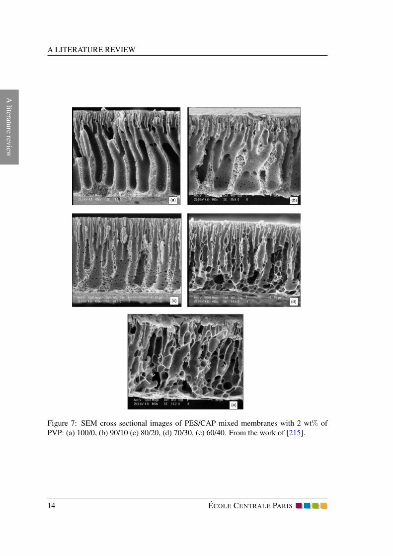
wFigure 9: Concentration polarization, cake formation, and internal adsorption phe-
nomenon in a crossflow filtration process.
ECOLE CENTRALE PARIS 19

Aliteratu
rerev
iew
A LITERATURE REVIEW
During the pressure-driven filtration processes through a membrane, particles/solutes are
transferred by convective force to the membrane surface. Subsequently they are partly
retained on the surface or passed through the membrane. The accumulated solutes will
gradually form a thin layer adjacent to the membrane surface generating a concentration
gradient. In other words, the concentration of solutes at the membrane surface is higher
than the bulk fluid. This phenomenon is called concentration polarization (CCP ) and
increases the hydraulic resistance to the permeate flow. Concentration polarization is a
reversible phenomenon and can be eliminated by simple water rinsing from the membrane
surface.
When the solute concentration attain a critical value on the membrane surface a gel-
like cake forms on the membrane surface. This gel layer arises when the concentration
at the membrane surface due to concentration polarization (CP) reaches the solubility
limit of the solutes.This phenomenon is called cake formation (CCake) and increases the
membrane resistance to the permeate flow. Cake formation can partly be removed from
the membrane surface by physical-chemical membrane cleaning.
Solutes with smaller size than membrane pores will pass partially through the membrane.
They either block completely the pores or adsorb to the internal membrane pores result-
ing in a reduction of the membrane internal pore size. This phenomenon is called internal
blocking (Cin) and is counting for the irreversible fouling which can not be treated by
membrane cleaning procedures [5],[53], [31], [178], [218]. In internal blocking, adsorp-
tion refers to a surface phenomenon occurring at the membrane interface.
Despite the fact that membrane fouling is the inevitable phenomenon occurring in all
filtration processes, some strategies can be adapted in order to minimize the loss of the
membrane performance.The membrane-solutes interaction/affinity is one of the important
factors on the membrane fouling. Thus, the first useful strategy consist of the character-
ization of the feed solutions (nature, charge, pH) and then choosing a membrane which
is less likely to be fouled. The operational conditions also play an important role on
the particle deposition on the membrane surfaces. For instance, in cross flow filtration
processes, the tangential bulk flow to the membrane surface destabilizes the particle ac-
cumulation and partly remove them from the membrane surface. High feed flow velocity
and/or use of spacers in spiral membrane modules can also increase the shear stress and
turbulence near the membrane surface and reduce the fouling pattern. Conventional phys-
ical/chemical cleaning procedures are also useful to remove the reversible and irreversible
fouled layers during the filtration processes.
1.3 MEMBRANE BIOFOULING
Several membrane processes with industrial applications (wastewater treatment, food sec-
tor) include filtration of mixed solutions (microorganisms, suspended particles, natural
organic matter, solutes, ions, surfactants, etc.)[10]. During the filtration of solutions con-
taining microbial cells, not only the classical fouling mechanisms exist (concentration
polarization, adsorption, pore blocking), but also the irreversible attachment of microbial
20 ECOLE CENTRALE PARIS

1. A LITERATURE REVIEW
Ali
tera
ture
revie
w
cells to the membrane surface leads to biofilm formation. Biofilm is a complex hydrated
matrix of microbial cells entrapped in an extracellular polymeric substances (EPS). EPS is
composed of polysaccharides, proteins, humid acids, nucleic substances, etc. (see section
1.5.8). Biofouling is inherently more complicated than other membrane fouling phenom-
ena because in one hand it consists of a dynamic process in which microorganisms can
grow, multiply, and relocate and in the other hand secreted substances from the matrix can
adsorb on/block the membrane pores. in other words, biofilm counts for a progressive hy-
draulic resistance both in the membrane pores and on the membrane surface. Therefore,
biofouling during the membrane filtration has been studied in the past decades and mod-
els have been proposed to predict the evolution of permeate flux, membrane permeability,
solute transport and biofilm growth [41], [55],[67],[92] [120]. The models mainly provide
a vision of the overall membrane performance and do not include pore scale information
of mass and momentum transport inside the membranes and the biofilms. However, it is
important to understand properly all interactions involved with biofouling in oder to de-
velop a model in which local mechanisms of mass transport would be taken int account.
For this reason, in next sections, membrane filtration of protein solutions in literature will
be briefly reviewed and important parameters of protein-membrane interactions will be
determined. Then, biofilms will be introduced and important parameters on their devel-
opment will be given respectively.
1.4 MEMBRANE FOULING BY PROTEINS
Natural organic matter (proteins, polysaccharides, humid substances) are mainly
responsible for membrane fouling and consequent permeate flux decline in filtration
processes[125], [135],[157],[186]. Consequently the membrane rejection properties
are irreversibly modified. Therefore, membrane filtration processes of proteins and
macromolecules have been vastly studied in the past decades in order to give a better
vision of the membrane performance of the membrane and fouling mechanisms in
function of time.
It is often supposed that fouling of macromolecular solutions is only caused by the
gel formation (cake) and concentration polarization on the membrane surface. The cake
formation or concentration polarization theories are often used to describe the tempo-
ral evolution of transmembrane pressure, permeate flux and solute transfer through the
membrane. It is obvious that models must take into account all important properties of
macromolecules and their interaction with the membrane surface. However, one impor-
tant factor that is not included in most models is the ability of macro solutes to adsorb at
almost any solid interface.The adsorption on the membrane surface is probably the first
step in the fouling process and could have great effect on the membrane characteristics.
In the work of [148], [149]. Therefore, another aspect of fouling modeling that has re-
cently received attention is macromolecular adsorption to the membrane. The adsorption
affects both the hydraulic permeability and the rejection properties of the membrane. In
ECOLE CENTRALE PARIS 21

Aliteratu
rerev
iew
A LITERATURE REVIEW
Table. 3, a summary of filtration experiments of BSA solutions with different membranes
at different operational conditions has been given.
In the work of Matiasson [160], it was shown that the BSA adsorption would reduce
5% of permeate flux for the cellulose acetate membranes and up to 35% of performance
for the polysulfone and polyamide membranes. From this results, it is clear that ad-
sorption has an important role in the flux reduction of filtration processes. Moreover the
adsorption kinetics of BSA have been studied. The agreement between the adsorbed BSA
amount and the increase in hydraulic resistance in function of time is quite good. It was
also shown that after 10 minutes, the adsorption of BSA on cellulose membranes would
attain the saturated value, while this took around 1 hour for the polysulfone membranes.
The results also indicate that there are at least two distinct steps in the adsorption process
of BSA on different membrane components notably a rapid adsorption step followed by
more slow step which both increase the hydraulic resistance of the membrane.
In the following, a brief description of parameters affecting the protein adsorption on
membrane surface including the chemical properties of the solution, membrane properties
and properties of the proteins is given. In Table 3, different studies on the filtration of
proteins with specific objectives are presented.
1.4.1 CHEMICAL PROPERTIES OF THE PROTEIN SOLUTIONS
Chemical properties of the protein solutions (pH, ionic strength) influence significantly
the membrane fouling by proteins. The solution charge, affects the protein conformation,
stability, membrane-protein interactions and tendency of the proteins to deposit to the
membrane surface. Moreover, pH of the solution plays important role on the effective
protein’s size and can also modify the protein-membrane interactions resulting into more
or less adsorption/desorption rates. In literature, a number of studies studies the protein
filtration at different values of pH[5], [34], [79], [99], [115], [169], [186],[193]. It has
been shown that proteins adsorption is maximal at its isoelectric point (IEP). When the pH
equals the isoelectric point (pI)of a protein the number of negative and positive charges
are in balance resulting in a net neutral molecule. The electrostatic protein-protein repul-
sions are minimum at isoelectric point allowing higher adsorption densities on the surface
[35]. Burn and Zydney [42],[62] investigated the effect of solution pH on the transport
of globular proteins on PES membranes; the results show a maximum protein-sieving
coefficient near the isoelectric point (IEP) of proteins. The non-linear dependance of the
sieving coefficient on pH was seemed to be a reason as the non-linear dependance of BSA
charge on the solution pH. Moreover, attractive electrostatic interactions occurred when
the protein and membrane had large opposite charges.
The ionic strength of the protein solutions is another controlling parameter in the ad-
sorption phenomena. The ionic strength basically determines the Debye length correlat-
ing with the damping distance of the electric potential of a fixed charge in an electrolyte.
That means the higher the ionic strength the shorter are the electrostatic interactions be-
tween the charged particles. As a consequence the adsorption of charged proteins to op-
22 ECOLE CENTRALE PARIS

1. A LITERATURE REVIEW
Ali
tera
ture
revie
w
Tab
le3:
Are
vie
wof
inves
ted
appro
aches
on
mem
bra
ne
filt
rati
on
by
pro
tein
solu
tions.
Pro
tein
Ran
ge
of
conce
ntr
atio
n
(g/L
)
Mem
bra
ne
type
Mem
bra
ne
com
posi
tion
Obje
ctiv
esR
ef.
BS
A,L
yso
zym
e,
Glu
tam
icum
,H
um
icac
id0-4
0
MF
/UF
/
NF
/RO
PE
S,A
mic
on,
PS
U,
poly
amid
e,
Poly
carb
onat
e
(TE
),ce
ram
ic
Solu
tion
chem
istr
y(p
H
and
ionic
stre
nght)
effe
cts
on
mem
bra
ne
fouli
ng
[62
],[7
9],
[169],
[187],
[ 116],
[168],
[142],
[193],
[8]
BS
A,D
extr
an0.5
-2M
F/R
O
Mix
edce
llulo
se,
poly
amid
e
Oper
atio
nal
conta
ins
(TM
Pan
dfl
owvel
oci
ty)
effe
cts
on
mem
bra
ne
fouli
ng
[111],
[110],
[ 266]
Lyso
zym
e,C
yto
chro
me,
Myoglo
bin
,H
emoglo
bin
,
BS
A,P
epsi
n
β-l
acto
glo
buli
n
α-l
acta
lbum
in0-2
MF
/UF
Cel
lulo
se,P
ES
,
Poly
carb
onat
e
(TE
)
Infl
uen
ceof
single
or
bin
ary
pro
tein
mix
ture
s
on
mem
bra
ne
fouli
ng
[132],
[190],
[180]
BS
A1-1
0M
F
Poly
carb
onat
e
(TE
)
Obse
rvat
ion
of
succ
essi
ve
fouli
ng
step
s
duri
ng
filt
rati
on
pro
cess
[99
],[3
3]
C-l
abel
led
BS
A,B
SA
Ova
lbum
ine
0-1
0U
F/M
F
PV
P,N
ylo
n,
PE
S,
PV
DF,P
SU
Infl
uen
ceof
mem
bra
ne
nat
ure
on
mem
bra
ne
fouli
ng
[218],
[112],
[95
],[1
84],
[174]
C-l
abel
led
BS
A,B
SA
1-1
0M
F/U
F
Cel
lulo
se
acet
ate,
PS
U,
PE
S
Det
erm
inat
ion
of
the
hydra
uli
cper
mea
bil
ity
of
foule
dla
yer
s[1
86],
[162]
BS
A0.5
-2.5
UF
PE
S
Det
erm
inat
ion
of
the
effe
ctiv
edif
fusi
vit
yof
pro
tein
sth
rough
the
mem
bra
ne
[222],
[223]
ECOLE CENTRALE PARIS 23

Aliteratu
rerev
iew
A LITERATURE REVIEW
positely charged substrates is restrained whereas the adsorption to like-charged surfaces
is increased. Moreover, high ionic strength conditions increase the tendency of proteins
to form aggregates [241].
Temperature has a double effect both on the equilibrium state and on the kinetics
of protein adsorption. Increased adsorption rates can be expected due to acceleration
of protein diffusivity towards the sorbent surface. The major driving force of protein
adsorption is an entropy gain arising from the release of surface adsorbed water molecules
and salt ions and from structural rearrangements inside the protein [97],[153],[181]. As a
result the amount of surface adsorbed proteins increases in general at high temperatures.
1.4.2 INFLUENCE OF PROTEIN PROPERTIES ON PROTEIN ADSORPTION
Proteins are complex biopolymers composed in average of 20 amino acids as monomeric
units plus some possible chain sides like phosphides, oligosaccharides or lipids intro-
duced after translation. A classification of proteins with respect to their interfacial be-
havior can be archived by considering properties like size, structural stability and com-
position. The group of proteins called hard proteins (Lysozyme, β-Lactoglubin) sug-
gesting a generally little tendency to structural modifications after adsorption upon solid
surfaces [183], [182]. Intermediate size proteins such as Albumin, Transferrin, Immuno-
golubins are usually able to undergo some conformational reorientations once contacting
a solid surface. The couplex structure of these proteins can be decomposed into individ-
ual domains exhibiting specific properties like hydrophilic/hydrophobic, polar/non-polar,
or charged/uncharged parts [7]. The class of high molecular weight proteins include
polymer-like lipoproteins and glycoproteins are structurally labile and therefore show a
strong affinity to hydrophobic surfaces including significant conformational reorienta-
tions.
1.4.3 INFLUENCE OF SURFACE PROPERTIES ON PROTEIN ADSORPTION
Protein-surface interactions are influenced by the protein’s properties on one side and by
the surface properties on the other side. The important parameters to be considered are
surface polarity, charge, and morphology. The adhesion energy between proteins and
solid surfaces can be directly measured using atomic force microscopy (AFM) [77], [96],
[130],[131],[219]. It has been observed that proteins tend to adhere more strongly to non-
polar than to polar, to high surface tension than to low surface tension and to charged than
to uncharged surfaces [34]. In general, experimental results showed that proteins adsorb
more strongly to hydrophobic surfaces than hydrophilic ones. This can be explained by
the fact that there are less hydrogen bondings between water molecules and hydrophobic
solid surfaces which facilitate consequently the protein accumulation to solid surfaces.
24 ECOLE CENTRALE PARIS

1. A LITERATURE REVIEW
Ali
tera
ture
revie
w
1.4.4 PROTEIN ADSORPTION MODELS AT SOLID INTERFACE
When proteins approach a solid interface they typically behave like symmetric rigid par-
ticles that can either adsorb on or desorb from a surface. These two process were the
only ones taken into account in the Langmuir law where the theory of adsorption of gas
molecules on a solid surface has been developed [136]. This theory is still served to
develop the substantial description for the protein adsorption phenomena, however it is
too simplistic to match the complex behavior of the proteins. Protein secondary and ter-
tiary structures, protein orientation to the solid surfaces [124], structural rearrangements
after adsorption [165],[183], [252] and protein aggregation are parameters which should
take into account to develop comprehensive models for protein adsorption. However, it
is extremely complicated to develop a model taking into account all the mechanisms in
adsorption phenomena.
The simplest model existing is the linear model which relates the adsorbed quantity to the
equilibrium protein concentration near the solid surface.
θ = kc∗ (5)
In this model, θ is the adsorbed protein quantity, k is the adsorption constant which
includes the physicochemical properties of the substrate and the protein. The main prob-
lem of this model is that it accounts only for the adsorption process and hence it can not
be useful for prediction of desorption and/or final equilibrium state of adsorption phe-
nomena. The reference model in this field is the Langmuir adsorption model.
dθ
dt= kads · cs
(
1−θ
θmax
)
− kdes · θ (6)
In Eq. 6, θ refers to the protein coverage θmax is the maximum surface coverage, kads
and kdes are respectively the adsorption and desorption constants and cs is the protein
concentration in the vicinity of the solid interface. the adsorption of proteins from the
bulk solution causes a depletion of the surface concentration cs which in turn leads to a
protein transport from bulk solution to the region above the surface. As a consequence,
the surface concentration varies during the adsorption process.
Other models for description of protein adsorption are the Freundlich and Freundlich-
Langmuir (combination between Langmuir and Freundlich models). The empirical Fre-
undlich isotherm is employed to describe multilayer adsorption with interactions between
molecules on a heterogeneous substrate.
θ = k · cn (7)
Where θ is the adsorbed quantity at equilibrium, c is the concentration of proteins in the
solution, k is the relative sorption capacity, and n is an indicator of sorption intensity or
surface heterogeneity. The value of n indicates the degree of non-linearity between solu-
tion concentration and adsorbed proteins as follows: if n is equal to one, the adsorption
ECOLE CENTRALE PARIS 25

Aliteratu
rerev
iew
A LITERATURE REVIEW
is linear; if n is inferior to one, this implies that the adsorption process is chemical and
the surface is relatively homogeneous; if the value of n is more than one, adsorption is a
physical process and the sorbent is relatively heterogeneous.
Although these models are mostly used in almost every study invested in protein adsorp-
tion on solid interfaces, more complicated models have been also developed to describe
more detailed phenomena such as lateral interactions involved between proteins and solid
surface [34],[75], overshooting effects, irreversible and reversible adsorption [164], and
structural rearrangements during the adsorption [150].
1.4.5 PROTEIN QUANTIFICATION
In several filtration studies, proteins are quantified both in solution and on the membrane
surface in order to obtain the adsorption kinetic models, hydraulic resistance due to pro-
tein deposition and membrane rejection properties. Different technique are applied for
this purpose.
AFM is often applied to image the distribution of protein layer (aggregates) on a solid
surface. This technique can also be used to measure the structural rearrangement of indi-
vidual proteins. he limiting factor of many AFM studies is that imaging is after performed
after drying the surface which potsntially affects the folding state of the individual pro-
teins or the structure of the protein layer [2],[77].
The Fourier transform infrared spectroscopy (FTIR) with attenuated total reflectance
(ATR) mode is a sampling technique which enables samples to be examined directly in
the solid or liquid state without further preparation. ATR uses a property of total internal
reflection resulting in an evanescent wave. A beam of infra red light is passed through the
ATR crystal in such a way that it reflects at least once off the internal surface in contact
with the sample. The penetration depth into the sample is typically between 0.5 and 2
µm [65].The number of reflections depend on the angle of incidence. The beam is then
collected by a detector as it exits the crystal.
Recently, FTIR-ATR is applied to characterize the composition of organic membranes,
and the evolution of their composition or degradation and also the nature of fouling com-
ponents with time. The interest of using this technique, in studying the fouled membranes
with proteins, is the possibility of quantification of the clogging agents on the surface and
in the volume of the membranes. This is feasible by tracing a calibration curve for each
specific clogging agent. For this purpose, the known mass of the desired compound (in
solution) is deposed on the membrane surface and the corresponding infrared spectra are
obtained. The calibration curve consists of the amount of the specific component on the
membrane surface in function of the infrared spectra. later the quantity of the unknown
clogging agents on the fouled membranes can be determined[66],[222],[223].
In several studies, protein concentration in protein solutions is directly measured by
ultraviolet-visible spectrophotometer absorption. In the work of [222],[223], BSA con-
centration in solution has been measured at λ = 277nm. Combination of calorimetric
methods with spectrophotometer absorption has also been used for determining the total
26 ECOLE CENTRALE PARIS

1. A LITERATURE REVIEW
Ali
tera
ture
revie
wFigure 10: Penetration of IR beam in a sample:successively fouling layer (thickness
∼ 1− 10µm)/active layer of membrane (thickness ∼ 200 nm) and support layer of mem-
brane,from the work of [66].
ECOLE CENTRALE PARIS 27

Aliteratu
rerev
iew
A LITERATURE REVIEW
protein concentrations in a mixture [44]. These methods are based on the reaction of
chromophore agents with the peptide bonds or with certain amino acids of the proteins.
The reaction yields coloration (in the visible region) in which intensity (absorbance) is
directly proportional to the protein concentration [1]. The most used methods in this field
for protein quantification are Biuret, Lowry and Bradford. In the work of Kimberly et
al. [116], UF membranes were immersed in surfactant (SDS) solutions. The adsorbed
proteins were deorbed in surfactant solution. A micro-lowry method is then applied to
measure the protein concentration.
1.5 BIOFILMS
A biofilm is an assemblage of microbial cells that is irreversibly associated with a sur-
face (not removed by gentle rinsing)and enclosed in a matrix of extracellular polymeric
material (EPS). This matrix is mainly composed of polysaccharides, proteins, polyuronic
and nucleic acids and lipids [64],[224]. The general composition of biofilms has been
determined by [234] and is summarized in Table 4.
Non-cellular materials such as mineral crystals, corrosion particles, clay or blood com-
ponents, depending on the environment in which the biofilm has developed, may also be
found in the biofilm matrix. It should be also pointed out that biofilm-associated organ-
isms also differ from the planktonic (freely suspended) counterparts with respect to the
genes that are transcribed.
Biofilms may form on a wide variety of surfaces including living tissues, indwelling
medical devices, industrial or potable water system piping or natural aquatic systems.
They are responsible for most microbial conversions in natural environments. Natural
biofilms can approximately develop on all kind of solid surfaces like rocks and plants in
seawater and fresh water and sediment grains. Consequently, biofilms have been associ-
ated with a wide range of problems both in industry and medicine and have been used
for various bioprocesses. Biofouling of heat exchangers, of industrial and drinking water
pipelines and medical devices have been reported. Additionally, biofilms also offer a huge
potential for biological wastewater treatment (domestic and industrial), bioremediation of
hazardous waste sites and leaching of metals.
Table 4: General composition of biofilm [234]Component % (mass) of matrix
Water up to 97%Microbial cells 2-5%Polysaccharides 1-2%
Proteins ≤1-2%DNA and RNA ≤1-2%
Ions and inorganic not known
28 ECOLE CENTRALE PARIS
1. A LITERATURE REVIEW
Ali
tera
ture
revie
w
Figure 11: Different stages of biofilm development:(1) Initial attachment, (2) Irreversible
attachment, (3,4) Maturation, (5) Dispersion. Adapted from the work of [57]
Three main process have been identified in biofilm development[?] and are shown
in Fig.11: initial attachment of the cells to the surface (colonization), growth of the at-
tached cells into a mature biofilm and production of extracellular polymeric substances
and detachment of single cells (erosion) or large pieces (sloughing off).
The initial attachment of microorganisms to the solid surface is a complicated process
depending on both surface and liquid physicochemical properties such as charge and
ionic strength of the liquid, surface hydrophobicity, roughness and charge, hydrodynamic
conditions of the surrounding liquid and the interfacial properties of the microorganisms.
See section 1.5.1.
In the following section, a brief description of the important physical and chemical pa-
rameters affecting biofilm development is detailed. A description of biofilm composition
and structure and mass transfer in biofilms is also given.
ECOLE CENTRALE PARIS 29

Aliteratu
rerev
iew
A LITERATURE REVIEW
1.5.1 IMPORTANT PHYSICOCHEMICAL PARAMETERS ON BIOFILM FORMATION
1.5.2 SUBSTRATUM EFFECTS
The solid surface may have several characteristics which can affect the attachment and
biofilm development. It has been noted [45] that the surface roughness appears to increase
the microbial colonization. The physiochemical properties of the surface may also have
a strong influence on the rate and the extent of attachment. It has been reported that
microorganisms attach more rapidly to the hydrophobic, nonpolar surfaces such as Teflon
and other plastics [25],[84],[204] than to hydrophilic materials such as glass. This can be
a result of some hydrophobic interactions between the cells and the surface which would
enable the cells to overcome the repulsive forces active within a certain distance from the
surface and irreversibly attach.
1.5.3 CONDITIONNING FILMS
A solid surface exposed in an aqueous medium will immediately and inevitably become
conditioned or coated by polymers from that medium, and the resulting chemical mod-
ifications will affect the rate and the extent of microbial attachment. Loeb and Neilhof
[144] have reported that these films were naturally organic and formed within minutes of
exposure, and continued to grow for several hours.
1.5.4 CHARACTERISTICS OF THE AQUEOUS MEDIUM
The characteristics of the aqueous medium, such as pH, nutrient availability, ionic
strength, and temperature may play a role in the rate of microbial attachment to a
substratum[72],[80]. It has been found that an increase in the concentration of several
cations (sodium, calcium, ferric ion) affected the attachment of Pseudomonas fluorescens
to glass by reducing the repulsive forces between the negatively charged bacteria and the
glass surface. [82],[83]. It has been also noted that an increase in nutrient concentration
can be correlated with an increase in the number of attached bacterial cells [55].
1.5.5 PROPERTIES OF THE CELL
Cell surface hydrophobicity, presence of fimbriae and flagella, and production of EPS
influence the rate of attachment of microbial cells. The hydrophobicity of the cell sur-
face is important in cell attachment because hydrophobic interactions tend to increase
with an increasing nonpolar nature of one or both surfaces involved. Most bacteria are
charged negatively but still contain hydrophobic surface components [220]. Fimbriae,
non-flagellar appendages, contribute to cell surface hydrophobicity. Fimbriae play a role
in cell surface hydrophobicity and attachment, probably by overcoming the initial elec-
trostatic repulsion barrier that exists between the cell and substratum. Other cell surface
properties may also facilitate the attachment process. Several studies have shown that the
treatment of adsorbed cells with proteolytic enzymes caused a marked release of attached
30 ECOLE CENTRALE PARIS

1. A LITERATURE REVIEW
Ali
tera
ture
revie
w
bacteria, providing evidence for the role of proteins in attachment[18],[58]. In 1971, Mar-
shall [158] provided evidence, based on SEM, that the attached bacteria were associated
with the surface via fine extracellular polymeric fibrils. Korber [133] used motile and
non-motile strains of P. fluorescens to show that motile cells attach in greater numbers
and attach against the flow more rapidly than the non-motile strains. Therefore, flagella
present on the surface of motile cells seem to play an important role in attachment. In
light of these findings, cell surface structure such as fimbriae, other proteins, LPS, EPS,
and flagella all clearly play an important role in the attachment process.
As a conclusion, attachment will occur more rapidly on surfaces that are rougher, more
hydrophobic, and coated by surface conditioning films. An increase in flow velocity,
water temperature, or nutrient concentration may also lead to increased attachment, if
these factors do not exceed critical values.
1.5.6 QUORUM SENSING
Cell-to-cell signaling has recently demonstrated to play a role in cell attachment, biofilm
development and detachment[264],[147]. By sensing cell-produced compounds, (e.g.,
N-acyl-homoserine lactones), cells recognize the local cell density (therefore called
”quorum-sensing”) and react by switching on or off certain sets of functional genes. It
has been proved that quorum-sensing determines biofilm structure. In the work of [59]
cell-to-cell signals are involved to produce a biofilm. At sufficient bacterial population
densities, these signals reach concentrations required for activation/mutation of genes
involved in biofilm formation, but unlike the wild type, their biofilms were much thinner,
cells were more densely packed, and the typical biofilm architecture was lacking.
1.5.7 BIOFILM STRUCTURE
1.5.8 EXTRACELLULAR POLYMERIC SUBSTANCES (EPS)
The proportion of EPS in biofilms can range from 50% to 80% of the total organic matter.
This is the main structural component of biofilms. The physical properties of the biofilm
are largely determined by the EPS while the physiological properties are determined by
bacterial cells.
As EPS were considered mainly composed by polysaccharides, many detection tech-
niques focus on this group of compounds [20],[52],[179]. However recent studies re-
vealed that proteins are the most abundant component in the EPS matrix (50% or even
more). Consequently, more research on the EPS composition is needed, since EPS has
been linked with many processes and properties integral to biofilm behavior: attachment,
detachment, mechanical strength, antibiotic resistance and exo-enzymatic degradation
activity.
Research also demonstrated that the composition and structure of EPS determine the
structure of biofilms and that the EPS in biofilms may vary spatially and temporally.
ECOLE CENTRALE PARIS 31

Aliteratu
rerev
iew
A LITERATURE REVIEW
It has been shown that the EPS matrix also affects solute’s diffusion in biofilms. Ac-
cording to [40], the diffusion of small molecules is not strongly inhibited by the biofilm
matrix, whereas the diffusion of large molecules are impeded.
Other studies focusing on EPS properties reported that the forces keeping the polymers
together in the matrix are not strong covalent bonds, but weak hydrophobic and elec-
trostatic interactions and hydrogen bonds. It is clear that further research is needed on
both physical and chemical properties of EPS which appears to play a critical role in the
structure and activity of biofilms.
1.5.9 HETEROGENEITY
Biofilm structure is the spatial arrangement of microorganisms, cells clusters and EPS and
eventually solid particles. Since the structure affects solute’s transport, it is a significant
determinant in the activity of the biofilm.
Despite the initial reports of biofilms as planar and homogenous structures, recent micro-
scopic observations indicated that biofilms are not flat and the distribution of microorgan-
isms is not uniform. Instead, multispecies biofilms were observed with complex struc-
tures, heterogeneous both in space and time, containing voids, water channels, cavities
and with cells arranged in clusters or layers[230]. Biofilms have been considered to be
highly porous polymer gels and diffusion studies of [52] demonstrated their gel-like char-
acteristics.
Depending on growth conditions and age, the biofilm thickness can vary from a few
micrometers up to a centimeter [23].
Density, volume fraction of water phase (porosity) and tortuosity of biofilms change with
biofilm depth, showing biofilm heterogeneity (see section 1.5.10). The non-uniform dis-
tribution of these parameters also affects the mass transfer mechanisms inside biofilms.
Owning to the microscopic dimensions of biofilms, their structural analysis strongly de-
pends on the microscopic methods used. Most microscopic techniques for structural char-
acterization of biofilms involve preparation of samples, such as dehydration and embed-
ding, which causes damage to the soft biofilm structure biofilm-microscopic-methods.
After the introduction of confocal scanning laser microscopy (CSLM), biofilm struc-
ture perception changed drastically. CSLM images revealed that biofilms can consist
of biomass clusters separated by interstitial voids [21]. It was also concluded from the
images that voids were water channels in connection with the bulk water phase. The
presence of voids has considerable consequences for mass transfer inside the biofilms
(convection) and exchange of nutriments and products with the water phase.
32 ECOLE CENTRALE PARIS

1. A LITERATURE REVIEW
Ali
tera
ture
revie
w
Table 5: List of microscopic techniques for studying biofilms
Microscopy
technique
Spatial
resolution Application Sample treatment References
LM 1µm EPS and cells
Dehydration, freezing,
sectioning, staining [48]
FM 1µm EPS and cells
Dehydration, freezing,
sectioning, staining
[20], [205],
[92]
TEM 1 nm Cells and EPS
Dehydration, sectioning,
staining [16], [19]
SEM 1 nm
Cell and EPS
surfaces
Dehydration, sputter
coating [19]
ESEM 10 nm
Celle and EPs
surfaces None [192]
CSLM 1µm EPS, cells, voids staining [22], [139]
AFM 0.1µm
Cell and EPS
surfaces None [37], [93]
Abbreviations: LM: light microscopy; FM: fluorescence microscopy; SEM: scanning
electron microscopy; ESEM: environmental scanning electron microscopy; CSLM: con-
focal scanning electron microscopy; AFM: atomic force microscopy.
1.5.10 DENSITY, POROSITY AND HYDRAULIC PERMEABILITY OF BIOFILMS
In the work of Zhang [269], the spatial distributions of biofilm density, porosity and mean
pore radius were determined with biofilm depth using experimental data and modeling
approaches.
The volume fraction of water or the porosity of biofilm is defined as the portion of a
biofilm occupied by water outside of the cells[246]. In this work, biofilm porosities
change from 84-93% in the top layers to 58-67% in the bottom layers.
Additionally, an average dry density of the biofilm of 1.17 mg-TS/cm3 (TS means Total
Solids) dry biomass was measured. On the other hand, the wet densities of biofilms in-
creased from 1.001-1.003 g-TS/cm3 in the top layers to 1.01-1.02 g-TS/cm3 in the bottom
layers. The density in the bottom layers were 5-10 higher than those in the top layers.
This corresponds to the increase of the TS with depth (observed in this study) indicating
that cells are more densely packed in the bottom layers. This is also in agreement with
the decrease of the porosity with depth.
In contrast, the biofilm mean pore size decreased from 1.6-2.4 µm in the top layers to
0.3-0.4 µm in the bottom layers[269].
ECOLE CENTRALE PARIS 33

Aliteratu
rerev
iew
A LITERATURE REVIEW
Hydraulic permeability is another major parameter characterizing a porous biofilm
medium. It has been shown to depend on the relative content of cells and gel-like
polymeric matrix ([163]. Moreover, Fowler and Robertson [86] suggested that the ability
of cells to move with respect to one another in immobilized bacterial cell aggregates
affected the hydraulic resistance of this bacterial medium. In the work of 83, values of
biofilm hydraulic permeability and porosity of 10E-16 m2 and 0.8, respectively were
reported.
1.5.11 DISPERSAL
Biofilm cells may be dispersed either by shedding of daughter cells from actively growing
cells, detachment as a result of nutrient limitation or quorum sensing, or shearing of
biofilm aggregates (continuous removal of small portions of biofilm) because of flow
effects [71].
The mechanisms underlying the process of shedding by actively growing cells in a biofilm
are not well understood. It has been shown that the surface hydrophobicity of newly di-
vided daughter cells spontaneously dispersed from biofilm differ substantially from ma-
ture cells in biofilm. These differences might explain the detachment of newly divided
daughter cells. Hydrophobicity was reported lowest for the newly dispersed cells.
Detachment caused by physical forces has been studied more in detail. The importance of
physical forces in detachment has been proved. The three main processes for detachment
are erosion or shearing (continuous removal of small portions of the biofilm), sloughing
off (rapid and massive removal), and abrasion (detachment due to collision of particles
from the bulk with the biofilm). It has been noted that the rate of erosion from biofilm
increases with the biofilm thickness and fluid shear at the biofilm-bulk liquid interface.
Sloughing is a more random process and is thought to be a result of nutrient or oxygen
depletion within the biofilm structure. Sloughing off is more commonly observed with
thicker biofilms that have developed in nutrient-rich media.
The mode of dispersal may evidently affect the phenotypic characteristics of the organ-
isms. Eroded or sloughed aggregates from the biofilm are likely to retain certain biofilm
characteristics, such as antimicrobial resistance properties, whereas cells that have been
shed as a result of growth may revert quickly to the planktonic phenotype.
1.5.12 MASS TRANSFER AND MICROBIAL ACTIVITY
Substances for biofilm growth are usually supplied by the water phase, and metabolic
products are eventually released into the water phase. The rates of exchange between the
biofilm and the water phase are determined by the mass transfer processes of diffusion
and convection. It should be pointed out that microbial conversions in biofilms, related
mostly to cell growth and division, are dependent and often limited by mass transfer.
A common property of microbial biofilms is resistance for mass transfer of different so-
lutes. This is due to the limited water flow inside the matrix and the presence of a hy-
34 ECOLE CENTRALE PARIS

1. A LITERATURE REVIEW
Ali
tera
ture
revie
w
drodynamic boundary layer between the matrix and the surrounding water phase [117],
[118],[203].
Transport of solutes is thought to be primarily by diffusion inside the biofilm matrix and
in the boundary layer near the solid surface. Consequently, when the internal chemical
composition (substrates and products) differs from the bulk medium, steep gradients de-
velop. This has strong effects on the type and the rates of microbial conversions within
the biofilm.
The simplest biofilm concept is a planar geometry with microbial activity distributed ho-
mogeneously and constant transport parameters regardless of biofilm depth. The biofilm
surface is separated from the mixed bulk liquid by a mass boundary layer (MBL) in which
the transport of species gradually changes from diffusion (biofilm) to convection (bulk
liquid). This is illustrated in Figure 2 presenting the O2 micro-profile in and above an
active biofilm. This concept is simple and facilitates mathematical modeling of transport.
The mass transfer resistances can be separated into external, in the MBL, and internal, in
the biofilm matrix. The resistance in the MBL is proportional to its thickness δ as shown
in Fig. 12, which mainly depends itself on the velocity of the fluid phase surroundingg
the biofilm matrix. The mass transfer coefficient ks and the thickness of the MBL can be
calculated by the liquid flow velocity [226].
ks = 0.0889u∞Sc−0.704 (8a)
Sc =ηρ
Deff
(8b)
With Sc as the Schmidt number, η as the dynamic viscosity, ρ as the density of the water
phase and δ = Deff/ks.
Both diffusion and convection of solutes are important when considering transfer phe-
nomena in biofilms. They are both hindered by the biofilm matrix; obviously the matrix
is an effective barrier not only for water movement (convection) but also for the random
movement of solutes (diffusion).
Internal mass transfer is usually considered to be diffusional and frequently described
using a single effective diffusion coefficient (Deff ). Diffusion is the only transport mech-
anism when there is no flow inside the biofilm matrix, however convection becomes the
dominant mechanism when the matrix is sufficiently permeable to allow the liquid flow.
Solute transport due to convection equals the velocity of the liquid inside the biofilm, and
even if it is in the order of 1 µm.s−1, convection is as important as diffusion for biofilms,
which typically range from a few hundred µm to several mm thick.
As previously reported, microscopic observations indicate that biofilms can be highly
porous, thus the common assumption that diffusion is the only transport mechanism must
be treated carefully.
Numerous studies reporting measurements of the Deff of several compounds in biofilms
have been reviewed. Literature values show a wide range of variation Deff being 1-900
% of the diffusion coefficient in water Dw. This reflects the variety of biofilm studies
ECOLE CENTRALE PARIS 35

Aliteratu
rerev
iew
A LITERATURE REVIEW
Figure 12: Oxygen profile measured in an active biofilm demonstrating that a significant
part of the mass transfer resistance occurred out side the biofilm adopted from the work
of De Beer [23]
as well as the different measurement methods. The Deff/Dw ratios for small molecu-
lar weights such as oxygen, glucose and nitrate in growing biofilms are assumed to be
around 0.9 [52]. Diffusion of macromolecules such as DNA, dextrans and proteins may
be more strongly influenced by biofilm matrices. This is due to the gel-matrix polymers
obstructing diffusion of macromolecules.
To describe transport inside biofilms, transport in the voids (diffusion and convection) and
in cell clusters (diffusion only) must then be distinguished and considered when studying
biofilms. For this purpose, measuring techniques with high spatial resolution are needed
and described in the literature[23].
1.5.13 EXPERIMENTAL CHARACTERIZATION OF BIOFILMS: MICROSCOPIC AND
STAINING METHODS
As previously reported, most microscopic methods (Fig.5) involve some preparation of
the sample, including staining, fixation, freezing, dehydration, embedding and section-
ing. As biofilms are soft structures mostly consisting of water, the preparation procedure
may significantly change, destroy or deform the matrix. As a result, in most cases, there
is an underestimation of the spatial heterogeneity. EPS appears as strands connecting
the cells. EPS morphology changes by dehydration: diffuse polymeric matter is con-
densed to strands, leading to overestimation of the pore-size. According to a study of
36 ECOLE CENTRALE PARIS

1. A LITERATURE REVIEW
Ali
tera
ture
revie
w
citebeeftink1986), from SEM images the pore-size appears to be in the order of 1µm
whereas TEM preparations show a pore size of 100 nm.
Figure 13: SEM image of biofilm formation by Escherichia coli from [9]
Images acquired by environmental scanning electron microscopy (ESEM) [143] and
atomic force microscopy (AFM) [36] (no dehydration) do not reveal the biofilm het-
erogeneity, but rather a smooth smear. A possible disturbing artifact from ESEM is the
filling of voids by water and drowning the roughness elements of the surface.
Figure 14: ESEM image of biofilm formation on (a) aluminum foil, (b) copper foil,
(marker 5mum) [143]
Confocal laser scanning microscopy (CSLM) is one of the tools most widely used at
present to study biofilm because it enables the direct in situ and non-destructive investi-
gation of native multicellular structures using specific fluorescent stains.
ECOLE CENTRALE PARIS 37

Aliteratu
rerev
iew
A LITERATURE REVIEW
Figure 15: Visualization of Shewanella cells labeled with green fluorescence protein
(GFP) using confocal laser-scanning microscopy (CSLM) in different times, (A): After
1h, (B) 8h, (C) 16h, (D) 24h, (E) 48h, (F) 120h. The first 3D construction of biofilm was
done after 12h. from the work of [236].
Specific staining is an important tool to determine the spatial distribution of different
biofilm components, most importantly in cells, EPS and voids. For viewing cells, non-
specific stains for DNA, such as acridine orange, diamidino-phenylindole (DAPI), ethid-
ium bromide and hexidium iodide are most useful. These dyes can also be combined
with confocal microscopy for giving of cell distribution in undisturbed biofilms. Stain-
ing of EPS for fluorescent microscopy or CSLM is also possible for proteins (fluorescein
isothiocyanate) and polysaccharides (lectin conjugates).
The recent development of image analysis software’s also provides an opportunity to ob-
tain detailed quantitative structural parameters on biofilms directly from confocal image
stacks. Structural parameters such as porosity, thickness, biovolume, substratum cover-
age by cells and EPS have been determined in several studies [38], [126].
1.6 MEMBRANE-BIOFILM FOULING MODELS
1.6.1 MEMBRANE FOULING MODELS
Modeling of the membrane fouling has been investigated in several sturdies during the
past years[98], [114], [135],[233]. The classical models are used to describe the flux
decline during the filtration processes. These models are mainly based on the work of
Hermia [98] and consist of four main blocking mechanisms: complete pore blockage, in-
termediate pore blockage, pore constriction (standard blocking) and cake filtration. These
38 ECOLE CENTRALE PARIS

1. A LITERATURE REVIEW
Ali
tera
ture
revie
w
Figure 16: Fouling mechanisms described by Hermia: (A) Complete blocking, (B) Pore
constriction, (C) Intermediate blocking, (D) Cake filtration.
mechanisms are presented in Fig.16. The mathematical expressions of these mechanisms
are also listed in Table. 1.6.1.
ECOLE CENTRALE PARIS 39

Aliteratu
rerev
iew
A LITERATURE REVIEW
Table 6: Mathematical expressions for classical fouling models
Model Governing equations Normalized flow rate
Complete pore blockage dAu
dt= −αQuCb
QQ0
= exp(
−α ∆pµRm
Cbt)
Intermediate pore blockage dAu
dt= −α
′
QuCbAu
A0
QQ0
=(
1 + α′ ∆pµRm
Cbt)−1
Cake filtration dRcake
dt= f ′R′JbCb
QQ0
=(
1 + f ′R′ 2∆pµR2
mCbt)−1/2
Pore constriction/Standard
blockingd(N0πr2pδm)
dt= −αinQuCb
QQ0
=(
1 + αinQ0
πr20δmCbt)−2
Abreviations: Au: Area of unblocked membrane (m2), Qu: Flow rate through unblocked
membrane area (m3/s), Cb: Bulk concentration (g/L), α: Pore blockage parameter, rep-
resenting blocked membrane area per unit mass of solutes convected to the membrane
surface (m2/kg), RP : Resistance of the deposits (m−1), f′
: Fractional amount of foul
ants contributing to solute deposition, R′
: Specific resistance of solutes (m−1), Jb Perme-
ate flux within the blocked area (m/s) , Rm Resistance of the clean membrane (m−1), rpRadius of membrane pores (m), δm: Membrane thickness (m). Adapted from [74].
In the complete pore blocking model, the permeate flow is drastically declined by particle
aggregation on the membrane surface and liquid flow can only pass through the unblocked
pore area. In this model, it is assumed that each particle reaching the membrane surface,
dispose on a free site of the membrane surface.Therefore, the rate of pore blockage is
function of permeate flow rate (Qu) and bulk concentration (Cb). The pore blockage pa-
rameter α represents the blocked surface per unit mass of aggregates deposited to the
membrane surface. The permeate flow decreases exponentially with time [98]. The inter-
mediate pore blocking model is similar to complete pore blocking model with additional
possibility of particle disposition on top of other particles already attached. In this model,
the particles does not necessarily block a pore but the probability of for a particle to block
a pore is evaluated. In this case, the rate of pore blockage is assumed to be proportional
to the ratio of unblocked surface to the total surface.
The cake filtration model assumes that a uniform cake layer is formed over the membrane
surface, and this fouling layer is permeable to fluid flow with resistanceRcake. In this case
particles locate on the other ones previously accumulated on the membrane surface and
new ones can not directly block the membrane surface. The cake layer resistance mod-
ifies with time and is proportional to the convective transport of formed aggregates to
the membrane surface (Jf ′Cb), where f ′ is the fraction of aggregates in the feed solu-
tion, and R′ is the specific cake layer resistance. The hydraulic resistance of cake layer
40 ECOLE CENTRALE PARIS

1. A LITERATURE REVIEW
Ali
tera
ture
revie
w
on the membrane surface by protein filtration (BSA) has been estimated in the work of
Mochizuki et al. [169] and Opong et al. [186].
The pore constriction model (standard blocking) takes into account the fouling which
occurs in the internal structure of the membrane. In this fouling mechanism, the column
occupied by membrane pores decreases due to particle deposit in the pore walls. The
rate of change of pore volume is proportional to the flow rate (Q) and bulk concentration
(Cb). Parameter αin denotes the volume of particles in the internal pores per unit mass of
protein filtered through the membrane.
Although, all these models provide a mechanistic description for each fouling progress,
significant differences between the flux decline data and model descriptions have often
been observed[81],[140],[238]. Consequently, a considerable number of studies devel-
oped combined fouling models accounting for coupled fouling mechanisms to describe
the flux decline. Ho and Zydney [102] developed a fouling model taking into account for
both pore blockage and cake filtration which was in good agreement with experimental
data obtained during bovine serum albumin (BSA) filtration using polycarbonate track-
etched membranes. De la casa et al. [62] developed a model by pore constriction and cake
formation model taking into account the electrostatic effects of the BSA solution to the
permeate flux. Fouladitajer et al. [85] studied the filtration of oil-water mixtures through
polyvinylidene fluoride microfiltration membranes. They obtained five combined fouling
models including different mechanisms. Moreover, Duclos-Orsello et al. [74] developed
a combined fouling model of complete blocking, pore constriction and cake filtration to
describe the flux decline through the microfiltration membrane.
Another approach of modeling the membrane fouling is a series of resistances su-
perimposing progressively to the membrane initial resistance for the solvent passage
throughout he membrane [14],[51], [110], [156], [239]. Depending on the filtration pro-
cess, one should take some or all the fouling mechanisms in the resistance series models
As presented in Eq. (9a) The permeate flux is proportional to the transmembrane pressure
and membrane initial resistance. However in a series of resistances to membrane resis-
tance would be the sum of resistances due to different fouling mechanisms (concentration
polarization (RCP ), cake formation (RCake) and internal blockage (Rin), see Eq. (9b).
Furthermore, each resistance is determined by empirical or semi empirical equations de-
pending on both solvent properties and operational conditions.
J =∆P
µRm
(9a)
J =∆P
µ(Rm +RCP +RCake +Rin)(9b)
In general, these resistances depend on the bulk concentration of particles, flow velocity,
particle concentration at membrane surface and shear stress. They can be estimated by
classical models (pore blocking, cake formation, etc.) or by empirical relations between
ECOLE CENTRALE PARIS 41

Aliteratu
rerev
iew
A LITERATURE REVIEW
parameters [239]. One possible way to estimate the polarization thickness layer (resis-
tance) is a film theory defined by Eq.(10). The polarization layer thickness can be used
both for determination of CP resistance individually [107] and in combination with other
fouling resistances [156].
δpol =D
vPln(
CP
Cb
) (10)
In this definition, D is the diffusion coefficient of solutes passing the membrane, vP is
the permeate velocity, CP and Cb are the concentration of solutes at bulk and membrane
surface respectively.
In parallel, numerical simulations of membrane models have been performed to compare
theoretical data with experimental data of the filtration processes. Rahimi et al. [214]
developed a 3-D CFD (computational fluid dynamics) model for predicting the water flux
through a microfiltration membrane. The experimental set up consisted of microfiltration
of blue indigo (insoluble in water) suspensions in a crossflow module. The pattern of par-
ticle deposition on the membranes has been studied at different hydrodynamic velocities.
The flow distribution in the porous membrane has been modeled based on Navier-Stokes
conservation equation for momentum and results from simulations have been used to
explain the experimental observations. It has been concluded that in higher crossflow ve-
locities, particles have less time to dispose to the membrane surface and thus the fouling is
less important. Ahmed et al. [6] obtained a 2-D theoretical CFD model to predict concen-
tration polarization, mass transfer coefficient and wall shear stress in a narrow membrane
channel. in the work of Bacchin et al. [13] a 2-D CFD model of mass and momentum
transfer was developed to describe the accumulation of colloids on membrane surface.
Numerical simulations integrated detailed modeling of physicochemical properties of the
colloidal dispersions (due to repulsive and attractive interactions at colloidal interface.
These interactions are fitted then to the CFD code. The model has been compared to
the experimental data which included filtration of latex particles through microfiltration
crossflow modules. Delaunay et al. [66] used the protein quantification of proteins by
FTIR-ATR on the membrane surface as an indirect proof of velocity and shear stress pro-
files in a complex geometry (porous membrane) and validated the experimental data with
CFD modeling approach. In the work of Marcos et al. [156], a 2-D model based on
a finite element method has been developed to simulate numerically the flow (mass and
momentum equations) and concentration of whey proteins in a hollow fiber. ultrafiltration
module.
1.6.2 BIOFILM MODELING
Among the problems associated with biofilms, energy losses, equipment damage, prod-
uct contamination and medical infections are generally reported. Understanding the in-
teractions between physical, chemical and biological phenomena on biofilm’s dynamics
is challenging and will help preventing damages caused by unwanted biofilms. In the
42 ECOLE CENTRALE PARIS

1. A LITERATURE REVIEW
Ali
tera
ture
revie
w
particular case of membrane systems, biofilm development induces a decline of process
performance. Consequently cleaning procedures and replacement of the membranes are
required.
Mathematical modeling of biofilms is therefore crucial to attain a broader and deeper in-
sight into those interactions and to assess the complex structure of the biofilm at different
steps of its development. Consequently, a huge number of studies have been invested in
this field for the last decades.
One critical point that should be taken into account when developing a biofilm model is its
structural heterogeneity both in space and time (see section1.5.9) Additionally, in biofilm
structure, very different length scales are presented. They vary from a few nanome-
ters (size of extracellular polymeric fibers), to several millimeters or centimeters (biofilm
thickness), with the size of bacterial cells (1- 2 µm) as an intermediate length scale.
Although it seems crucial to take into account a multi-scale description of a biofilm,
this strategy for biofilm modeling remains challenging for three main reasons:
• Experimental techniques can not characterize properly the biofilm structure at all
scales
• Computational resources are limited
• Not all the information provided at microscopic scale can be used at the macro-
scopic biofilm scale, thus the model can not be validated at microscale.
1.6.3 1-DIMENSIONAL CONTINUUM MODELS
The first attempts in biofilm modeling consisted in the development of continuum models
primarily in one space dimension [127],[216],[217],[249], [250]. These studies concen-
trated mostly on the steady-state biofilm growth dynamics including the biofilm thickness
and spatial distribution of microbial species and substrate concentrations. For instance
the model developed by Wanner and Gujer [246], based on a continuum description of
biofilms and the conservation of species, predicts the evolution of biofilm’s thickness,
dynamics and spatial distribution of microbial species and nutrients in the biofilm. It also
includes a biomass detachment mechanism due to shear stress and sloughing.
Single and multi-species biofilm were studied and modeled with this approach. Addi-
tionally, these continuum models also explain how the microbial composition and activ-
ity depend on the kinetics, nutrient concentration and other mechanisms such as initial
attachment and detachment.
However, the one-dimensional models significantly simplify the interactions between the
nutrients and biofilm and also the spatial dynamics of the biofilm. They also lack the
ability to characterize the multidimensional structure of the biofilm [245].
ECOLE CENTRALE PARIS 43

Aliteratu
rerev
iew
A LITERATURE REVIEW
1.6.4 DIFFUSION-LIMITED AGGREGATION (DLA) MODEL FOR BIOFILM GROWTH
AND PATTERN FORMATION
In general, the growth mechanism of the bacterial colonies is highly complex, in which
the substrate concentration plays an important role. One way to model this growth pattern
is the class of models called diffusion-limited aggregation (DLA) models.
The first biological DLA model described in the literature was a DLA model describing
the colony growth of Bacillus subtilis given by [87]. Later on, more experimental and
modeling studies were done [88],[161] .
The rule of DLA model is as follows: one chooses a seed particle as the origin of a square
lattice on a plane. Another particle is released far from the origin and is allowed to move
at random. When it arrives at the nearest neighboring site to the origin, it sticks to the site.
Then another particle is launched and it moves until it reaches the nearest neighboring of
a cluster made of the two particles. Through the repetition of these procedures, a cluster
grows with an outwardly open and randomly structure (Wang and Zhang, 2010).
Figure 17: DLA on compute simulation: (a) the rule of the 2D DLA growth. The solid
cell is the origin. The hatched cell is a new cell that has aggregated to the cluster. (b) a
typical example of a 2D DLA cluster which consists of 100000 particles, adapted from
the work of [237].
1.6.5 DISCRETE-CONTINUUM/CELLULAR AUTOMATON (CA) MODEL
The Cellular Automaton (CA) model consists of a regular grid of cells, each in one of a
finite number of states. The grid can be in any finite number of dimensions. The state
of a cell at time t is a function of discrete states of a finite number of cells at time t-1.
Every cell has the same rule for updating, based on the values of in her neighborhood.
Each time a set of rules are applied to the whole grid and a new generation is created. One
advantage of the CA model is its simplicity and the ability to produce a complex behavior.
It is then particularly attractive when simulating biological systems with heterogeneous
spatial structures [69],[257].
44 ECOLE CENTRALE PARIS

1. A LITERATURE REVIEW
Ali
tera
ture
revie
w
Figure 18: Modeling of the formation of a two species biofilm on a sphere in a mass
transfer limited regime using cellular automata adapted from[195].
CA models for biofilms incorporating the following phenomena : bacterial growth and
movement, cell to cell communication and the diffusion of nutrients [245]. These mod-
els can validate various biofilms growth profiles observed in experiments demonstrating
that the biofilm’s structure is significantly determined by the surrounding substrate con-
centration. Picionearu et al.[195] developed a combined differential-discrete CA biofilm
model, in which the nutrient concentration was assumed to be continuous and governed
by convectional diffusion-reaction equation. In this model the biomass density was com-
puted by a direct integration of the biomass balance equation, taking into account that the
growth is only the result of nutrient consumption. The biofilm spreading is modeled by
CA model and the newly formed biomass finds a place by pushing its neighbors and takes
the unoccupied space. Numerical simulations were carried out in 2D and 3D. Calculated
values of the global oxygen uptake rate, the concentration profiles for the oxygen, and the
biomass and the colonies size were both qualitatively and quantitatively in good agree-
ment with experimental data [61],[256]. It should be pointed out that in these models, the
effect of the surrounding bulk on biofilm growth, distribution or movement is not taken
into account.
1.6.6 BIOFILM MODELS WITH BIOMASS AND FLOW COUPLING
In most of the models presented previously, transport in the biofilm is only modeled by
diffusion and the effect of the surrounding bulk fluid is not explicitly coupled to biofilm
development. However, experiments confirmed that the hydrodynamics of the bulk fluid
plays an important role in shaping the structure of biofilms through both the convection
of nutrients and the detachment of biomass by shear stress [231],[232].
ECOLE CENTRALE PARIS 45

Aliteratu
rerev
iew
A LITERATURE REVIEW
Based on the previously established models and a better understanding of the biofilm’s
properties through experiments, several biofilm models coupled with bulk fluid were de-
veloped.
Picioreanu et al. [196], [197],[198] developed 2D and 3D hybrid discrete-continuum
models in which the flow over the irregular biofilm’s surface, convective and diffusive
mass transfer of nutrients, biofilm growth and biomass spreading were all taken into ac-
count. In this model, the biomass growth is modeled by the discrete CA (cellular automa-
ton) model, the mass balance of the substrate is modeled by the continuity equation and
the convection- diffusion-reaction equation, respectively. The flow field is governed by
the momentum balance (Navier-Stokes) equation.
The fluid flow affects the biofilm’s growth by both regulating the substrate concentration
at the biofilm-fluid interface and by shearing the biofilm’s surface. On the other hand,
the interaction is reciprocal since a new biofilm’s shape leads to a different boundary
condition and thus different flow and substrate concentration.
The set of governing equations for biofilm model development in work of [196] are given
below :
• The continuity equation for the fluid phase (incompressible)
∇ · u = 0 (11a)
• Momentum conservation for the fluid phase surrounding the biofilm (Navier-
Stokes)∂u
∂t+ u · ∇u = −
1
ρ∇p+ µ∇2u (11b)
• Mass conservation for the limited nutrient
∂CS
∂t+ u · ∇CS = −RS(CS, CX) +D∇2CS (11c)
• A kinetic equation for biomass growth
dCX
dt= RX(CS, CX) (11d)
In the work of [198] a two-dimensional model was developed where biofilm detachment
was considered. It was based on the internal stress created by a moving fluid in the
biofilm. Two detachment mechanisms, erosion (small-particle size) and sloughing (large-
biomass-particle removal) were modeled in this study.
Modeling studies reporting the effect of biofilm development on process performance are
also described in the literature. 2D and 3D models for assessing the effects of biofilm de-
velopment on the performance of spiral reverse osmosis membrane were also elaborated
by [210], [211], radu2010, [244]. These micro-scale models combine hydrodynamics
46 ECOLE CENTRALE PARIS

1. A LITERATURE REVIEW
Ali
tera
ture
revie
w
Figure 19: For a given biofilm geometry, (a) first the sub-domains, equations and bound-
ary conditions are defined, (b) the finite element mess is created. Next (c1) the hydro-
dynamics and mass transport of salt are simultaneously solved followed by (c2) the so-
lution of substrate transport and section. Based on the resulted substrate distribution
(d1+d2) the biomass grows and spreads according to the cellular automaton mechanism.
(d3) Mechanical stress in the biofilm is calculated and detachment steps are repeatedly
performed (remeshing after each step), followed by (d4) biomass attachment (newly at-
tached biomass). Finally, time is updated and with the newly obtained biofilm geometry
the whole cycle is repeated. [212]
ECOLE CENTRALE PARIS 47

Aliteratu
rerev
iew
A LITERATURE REVIEW
and mass transfer of solutes (salt and nutrients) with biomass attachment, biofilm growth
and detachment due to mechanical stress of liquid flow. Models were validated by experi-
ments. One example of model development (biofilm growth coupled with hydrodynamics
flow) algorithm is given in Fig.19.
Simulation results showing biofilm development on the spiral reverse osmosis membranes
are presented in Fig.fig.biofilm-development
1.6.7 UPSCALED MODELS FROM CELL-SCALE TO BIOFILM-SCALE
More recently, an increasing interest of the research community in considering the
multi-scale characteristics of a biofilm from the nanometer (EPS, protein in the matrix)
to the µmeter/centimeter (biofilm thickness)) in model development is reported[28],
[121],[122],[261].
The idea that biofilm models should be upscaled directly from microscopic scale has been
first proposed by Wanner and Gujer [247], [250]. The main advantages of the upscaled
techniques, in general, and the volume averaging, in particular, are the following: 1) the
resulting model relates the microscopic parameters to the observable macroscopic ones.
For instance, the effective diffusivity at macroscopic scale accounts for local diffusivities,
the microstructure and dispersion caused by the local velocity field; 2) upscaled equations
can be used in averaged continuos volumes. Volume averaging method is one of the
rigorous techniques for modeling of the porous media with different scales. Applying
averaging theorems associated with this technique, continuum equations for multiphase
are derived [255],[94]. This means that equations that are valid in a particular region
can be homogenized in order to derive equations that are valid everywhere, This way, a
discontinuous porous structure will be transformed to equivalent continuous media with
effective properties containing both local and structural properties of the porous medium
(See Fig.fig.voleme-av-method) .
In several studies upscaled models based on volume averaging method have been obtained
to describe the cellular reactive media including cellular growth, diffusion and reaction
in biofilms [60],[90],[188], [259] ,[260], [262]. More recently, the upscaled equations of
mass and momentum transport in the biofilm matrix have been derived [122].
In general, most of the works with the volume averaging method focused on local
mass equilibrium conditions in a representative elementary volume. Under these
circumstances, all intrinsic quantities (e.g. concentration, velocity field) can be assumed
to be equal in a representative elementary volume and one mass balance equation is
sufficient to describe mass and momentum transport. However, it should be noted
that non-equilibrium conditions with moving interfaces are closer to reality. However,
one should keep in mind that in the presence of an averaged behavior (e.g. biofilm
formation), the volume averaged can be applied and associated technical difficulties can
be overcome.
48 ECOLE CENTRALE PARIS

1. A LITERATURE REVIEW
Ali
tera
ture
revie
wFigure 20: General principles of the volume averaging method. Left: local porous
medium. Right: equivalent averaged medium with effective properties.
ECOLE CENTRALE PARIS 49

Aliteratu
rerev
iew
A LITERATURE REVIEW
1.6.8 MEMBRANE FILTRATION OF MIXED SOLUTIONS
As previously discussed, the main limitations of wild spread application of membrane
systems and optimization on their performance is membrane fouling leading to flux de-
cline and modification of properties (selectivity and retention). During the filtration of dif-
ferent mixtures, various interactions (hydrogen bonding, Van der Waals, ionic exchange,
etc.) are generated between the membrane and the particles/solutes. Recent studies are
mainly invested to understand the successive steps of the membrane fouling. [4], [12],
[62], [66], [74],[76], [156], [222], [235]. Electrostatic interactions between solutes and
membranes have been determined [62], [125],[166], [169],[186]. The complex morphol-
ogy of the membrane has been described in numerous studies [81], [215], [223]. All
these experimental observations are useful to provide data for advanced models which
are based on individual or combined mechanisms during a filtration process (biofilm for-
mation cake formation, concentration polarization, pore blockage, pore constriction and
series of membrane resistances). Up to now, the developed models for membrane fouling
are mostly macroscopic (at membrane scale) [56], [98], [156], [212], even though a lim-
ited number models are developed at molecular scale [253]. In molecular scale models,
a very high number of finite elements are needed in order to explain the local transport
mechanisms. This is not optimized in terms of time and cost. Moreover the molecular
scale models can only be validated macroscopically due to limitations of analytical meth-
ods. Therefore, an upscaled model based on the local description of the physical transport
mechanisms is useful to give a better vision of the overall behavior of the system includ-
ing both local and macrostructural information of the studied problem.
1.7 OBJECTIVES, ADAPTED STRATEGIES
The present work aims at studying the performance of a microfiltration membrane system
during filtration of solutions containing bacteria and to describe the consequent fouling
mechanisms.
During filtration, a biofilm develops on the membrane surface while the penetra-
tion/accumulation of secreted substances from the biofilm to the membrane internal
pores occurs simultaneously. As a result, an additional dynamic resistance (both on
membrane surface and in its volume) to the flow is formed which affects significantly the
membrane selective properties and permeate flux.
The diagram of the problem we intend to study in this work, in all its complexity, is pre-
sented in Fig. 21. It also describes the proposed modelling and experimental approaches.
As it is shown in Fig. 21, different length scales are presented in the global fouling
problem: from the mean pore size of the membrane (nm to µ m), proteins (several nm),
bacteria (1-2 µm) to membrane ( ∼ 200 µ m) and biofilm thickness (from a few up to
hundreds µm).
In the biofilm, three regions are considered at the local scale: cells, EPS and water chan-
nels. The transport mechanisms are convection and diffusion of species while reaction
occurs at the cell-EPS interface. In the membrane compartment, proteins are transported
50 ECOLE CENTRALE PARIS

1. A LITERATURE REVIEW
Ali
tera
ture
revie
w
Figure 21: Thesis objectives.
ECOLE CENTRALE PARIS 51

Aliteratu
rerev
iew
A LITERATURE REVIEW
by convection and diffusion to the membrane interface where protein adsorption takes
place. It should be pointed out that proteins are not the only species penetrating into the
membrane pores. Polysaccharides, humid substances, nucleic acids, DNA, etc. are also
present in the biofilm matrix, however, in order to maintain a simple system, we only
study protein adsorption to the membrane interface.
The objective of this work is to study the membrane system performance experimentally
and to propose two macroscopic (upscaled) models to describe the fouling of microfiltra-
tion membranes. In the first model, fouling due to protein adsorption to the membrane
pores is developed. The model is based on the transport phenomena at local scale. Gov-
erning equations of mass and momentum transport are given at this scale and boundary
conditions including adsorption at interface are set. The upscaled model is then obtained
using the volume averaging method. It provides averaged equations of mass and momen-
tum transport and the effective properties of the membrane (permeability and diffusivity).
The effective properties contain information of physical parameters at the pore scale along
with structural parameters at the membrane scale. Some numerical simulations are run
to evaluate the system performance qualitatively (more specifically the drastic changes
in the concentration fields in the fluid phase and in the membrane porous structure). In
parallel, experiments are specifically carried out to (1) get a better comprehension of the
fouling mechanisms by proteins and (2) provide parameters for both model development
at local scale and eventual validation that will be done in further work.
Membrane structural properties are obtained by a combination of analytical methods.
Scanning electron microscopy (SEM) images are coupled with two porosimetry tech-
niques (perfluoethers and mercury) in order to characterize the membrane. Three different
layers are detected. Thickness, porosity and the mean pore size are measured. The initial
membrane permeability is measured by filtration of milliQ water through the membrane.
Two proteins are chosen in this work: BSA (Bovine Serum Albumin) and L-Glutathione.
The physical-chemical properties of these molecules are significantly different. BSA is
a well-known protein which can correspond to the secreted macro molecules from the
biofilm. L-GLutathione is a small biomolecule (polypeptide) which can pass all through
the membrane. Experiments are carried out in order to determine the adsorption isotherms
laws for the two proteins. The membrane filtration of proteins is performed in a micro-
filtration module. The evolution of the permeate flux in function of time is evaluated for
solutions of each protein. The amount of adsorbed proteins on the membrane surface is
quantified by FTIR-ATR technique.
Finally, a preliminary upscaled model is developed to describe the mass and momen-
tum transport within the biofilm. A more realistic presentation of biofilms is taken into
account consisting of three regions (bacterial cells, EPS and water channels). Initial at-
tachment of bacteria, detachment caused by shear stress and biofilm growth are not de-
scribed in the model. At local scale, mass and momentum equations are described with
the appropriate boundary conditions. The cellular reaction takes place at cell-EPS re-
gion. The species (glucose, polysaccharides, oxygen, etc.) associated to cell metabolism
are supposed to be transported by convection and diffusion in the EPS matrix and wa-
52 ECOLE CENTRALE PARIS

1. A LITERATURE REVIEW
Ali
tera
ture
revie
w
ter channels. The solute transport to the cells is only described by diffusion. The volume
averaging method is also used to derive the upscaled equations. In general, upscaled mod-
els are mostly developed under the local equilibrium conditions. The effective properties
(permeability, diffusivity) of each biofilm region are expressed and can be calculated by
numerical solutions of the local closure problems. The effective properties contain some
additional information from both local (cell) scale and biofilm structure. The effective
permeability of the biofilm is then calculated from the results of the numerical simula-
tions in representative cellular regions with periodic flow conditions at the boundaries.
Experiments are necessary both at pore-scale (e.g. local diffusivity, porosity of each re-
gion) and biofilm-scale to provide local information to the model and subsequent model
validation. However, these experiments are not subject of the present work.
ECOLE CENTRALE PARIS 53


MICROFILTRATION MEMBRANE FOULING
BY PROTEINS : CHARACTERIZATION OF
MEMBRANE AND ADSORPTION 1
ECOLE CENTRALE PARIS 55

Chap
ter2
CHAPTER 1. MICROFILTRATION MEMBRANE FOULING BY PROTEINS :
CHARACTERIZATION OF MEMBRANE AND ADSORPTION
List of symbols
BSA Bovine serum albumine
C Bulk concentration (gL−1)
Cell Regenerated cellulose
J Permeate flux (Lh−1m−2bar−1)
Jw Permeate water flux (Lh−1m−2bar−1)
KBSA The equilibrium constant for BSA sorption (Lg−1)
MWCO Molecular weight cut off
PAN Polyacrylonitrile
PC Polycarbonate
PES Polyethersulfone
PVP Poly(vinylpyrolidone)
q Mass of protein quantified per per unit of apparent membrane
surface (µgcm−2)
q∗ Mass of protein adorned per unit of accessible membrane sur-
face (µgcm−2)
KmaxBSA Maximum sorption capacity for BSA (µgcm−2)
TMP Transmembrane pressure
T Temperature
αGlu(106Lcm−2) Linear adsorption constant for L-Glutathione
βGlu(µgcm−2) Linear adsorption constant for L-Glutathione
56 ECOLE CENTRALE PARIS

1. INTRODUCTION
Chap
ter
2
In this chapter, accumulation of organic matter on the membrane surface or into the
membrane pores and its influence on permeation during filtration on polyethersulfone
(PES) microfiltration membrane was studied. Two different organic compounds were
selected: Bovine Serum Albumin (BSA, 66 Kg mol−1, 583 peptides) and polypeptide
L-Glutathione (0.307 Kg mol−1, composed of three amino acids). The structure of two
polyethersulfone microfiltration membranes was characterized by scanning electron mi-
croscopy and porosimetry (perfluoroethers and mercury). Despite the same chemical
composition of the membrane, they presented different properties (pore diameter of ac-
tive layer and structure of the intermediate layer). One of these microfiltration membranes
was used to study the fouling behavior during the filtration process and to understand the
different fouling mechanisms due to adsorption, reversible and irreversible pore blockage
. Adsorption Isotherm experiments were carried out in static conditions. A linear adsorp-
tion isotherm was obtained for L-Glutathione (solution concentration:0-18 gL−1) and a
Langmuir isotherm for BSA (solution concentration: 0-24 gL−1). Isotherms developed in
dynamic conditions in the absence of the permeate flow and filtration experiments con-
firmed the linear adsorption of Glutathione whereas BSA presented lower adsorption rate
compared to the static tests. Local adsorption laws could be obtained from membrane
structure characterization and adsorption isotherms. For BSA solution of the relative per-
meate flux was linearly declined probably due to the accumulated mass of BSA on the
membrane during filtration. Additionally, reversibility of the fouling was studied for Glu-
tathione and BSA. Whereas Glutathione was totally desorbed from the membrane, results
from cleaning experiments performed in membranes fouled with BSA showed the pres-
ence of polarization concentration, reversible fouling, cleanable fouling and irreversible
fouling.
1 INTRODUCTION
1.1 CONTEXT
Membrane fouling is a complex mechanism associating accumulation of colloids, mineral
and natural organic matter (biomolecules like proteins and polysaccharides) and biofilm
development etc.
Although the nature of the fouling agents depend highly on the type of the solutions
to be treated, the natural organic matter (NOM) is well known to highly participate on the
membrane fouling in different filtration processes. Organic fouling may come from nat-
ural matter (humic acids), organic material coming from the filtered product or excreted
by microorganisms (proteins, polysaccharides) and specific pollutants. Porous membrane
fouling by organic matter occurs for example during water treatment (tap water produc-
tion, wastewater or industrial effluent treatment, grey water recycling), filtration of com-
plex media from food industry (milk, fruit juice, fermentation broth etc.). This paper
focuses on the fouling of microfiltration membranes by proteins and polypeptides. Clas-
sic modeling of membrane fouling usually take into account the following phenomena:
ECOLE CENTRALE PARIS 57

Chap
ter2
CHAPTER 1. MICROFILTRATION MEMBRANE FOULING BY PROTEINS :
CHARACTERIZATION OF MEMBRANE AND ADSORPTION
adsorption (accumulation of solutes on the external and internal surface, changing mem-
brane hydrophobicity and its pore diameter), pore blocking (accumulation of compounds
at the pore entrance, diminishing pore diameter), concentration polarization (rise of solute
concentration in the layer near the membrane surface) and cake formation (accumulation
of particles on the membrane forming a second porous media). It should also be noted
that depending on the particle membrane interactions (electrostatic interactions, hydro-
gen bonding, van der waals) the particle attachment to or accumulation on the membrane
surface can be reversible (removable by physicochemical treatments) or irreversible. Up
to now, several number of research works are based on Hermia description of fouling
[98]. Adsorption here is a generic word describing local interactions between membrane
material and solute from the bulk. In the context of protein/peptide filtration, the effect
of some parameters have been deepened [208]: nature and concentration of the protein
(or peptide) [5], [8], [89], [116], [129], [132], [175], [177], [184] membrane molecular
weight cut off and properties, filtration mode (cross-flow or dead-end filtration)[175], and
also the physicochemical properties of the solution through its pH and ionic strength [8],
[62], [78], [99], [116], [141],[159], [167], [175], [176], [177], [184], [187], [189], [191],
[193], [218], [266]. The physicochemical properties of the membrane can promote or pre-
vent protein adsorption. Among these properties, roughness, tortuosity, surface charge,
hydrophobicity and polarity are the main characteristics. It has been stated that the nonpo-
lar surfaces destabilize some proteins and thereby facilitate conformational reorientations
leading to strong inter protein and protein-surface interactions. This explains also the
general experimental results showing that proteins adsorb more strongly on hydrophobic
organic surfaces than onhydrophilic ones. Several studies investigated the effect of pH on
the amount of adsorbed protein on membrane surfaces and consequent membrane foul-
ing. It should be pointed that the pH determines the electrostatic state of proteins. When
the pH equals the isoelectric point (IEP) of a protein, the number of negative and positive
charges is balanced. The protein is then in neutral state. Since electrostatic protein-
protein repulsions are minimized at the isoelectric point, adsorbed protein densities were
found to be higher on the membrane surface at this pH. Additionally, the effective radius
of proteins also depends on pH and can significantly vary in function of it and with the
hydratation sphere, from 3.5 nm to 440.9 nm for Bovine Serum Albumin [62]. In sev-
eral studies, membrane performances (permeability, retention) have been investigated at
different electrostatic conditions (salt concentration). The ionic strength of the protein
solution is a controlling parameter on the protein adsorption. The ionic strength basi-
cally determines the Debye length correlating with the damping distance of the electric
potential of a fixed charge in an electrolyte. That means the higher the ionic strength, the
shorter the electrostatic interactions between the charged particles. As a consequence,
the adsorption of charged proteins to oppositely charged substrates is restrained whereas
the adsorption to like-charged surfaces is increased. Moreover, high ionic strength con-
ditions increase the tendency of proteins to form aggregates whilst they remain partly
soluble in the solution. Hydrodynamics can also affect the quantity and the quality of
protein adsorption on membranes. Convective forces increase the species accumulation
58 ECOLE CENTRALE PARIS

2. MATERIAL AND METHODS
Chap
ter
2
near the membrane surface [3, 38-40]. In this chapter, accumulation of proteins/peptides
on or into a microfiltration membrane of polyethersulfone (PES) was studied. The ef-
fect of proteins accumulation on membrane permeation during filtration of proteins in
one component solutions was also evaluated. Two different compounds were selected:
a large one, which is well known, Bovine Serum Albumin (BSA, 66 Kg mol−1). Thus,
results from this work can be easily compared with those of the literature. A small one
is also chosen, in order to get rid of eventual pore blocking or cake phenomena, and to
focus on adsorption: L-Glutathione (0.307 Kg mol−1). To facilitate the discussion, both
compounds will be called biomolecules in the rest of this chapter. It is worth to mention
that BSA exists in monomer and dimer forms, moreover the BSA molecules can form
aggregates in the solution which can cause immediate pore blocking on the membrane
surface. However all these effects have been neglected in this work and can be subject of
future studies. Experimental values of BSA accumulation on membrane during isotherms
in static conditions or filtrations from the literature are listed in Table.1.1 . To clarify, the
presentation includes only experiments with low ionic strength and near pH 7 (in which
BSA is negatively charged). A large dispersion of adsorption values is obtained, depend-
ing on the membrane (nature, pore size), the protein concentration, hydrodynamics, but
maybe also due to the analytical method. Several authors proposed to quantify BSA in
solution with UV analysis after desorption from the membrane by surfactant solutions.
This step introduces uncertainty on desorption and quantification of the protein. In this
work, proteins were directly quantified on membranes by FTIR methodology developed
by Rabiller-Baudry [66]. In the first part, two PES membranes were characterized. The
goal is to show the high variability of membrane structures. For one of the membranes, a
complete description of the whole porous media (active layer, intermediate layer and me-
chanical support) and of the whole active surface available for adsorption was obtained.
In a second part, the accumulation of BSA and L-Glutathione on this membrane was stud-
ied during isotherm in static and dynamic conditions, and during filtration experiments.
The impact of protein/peptide accumulation on the flux decline was analyzed for both
proteins.
2 MATERIAL AND METHODS
2.1 PROTEIN AND PEPTIDE
Bovine serum albumin (BSA) and L-Glutathione were supplied from Sigma-Aldrich. The
physicochemical properties of the proteins are listed in Table 1.2. The protein solutions
were prepared with milliQ water and stored in 4◦C. pH of the protein solutions was
7±0.4.
ECOLE CENTRALE PARIS 59

Chap
ter2
CHAPTER 1. MICROFILTRATION MEMBRANE FOULING BY PROTEINS :
CHARACTERIZATION OF MEMBRANE AND ADSORPTIONT
able
1.1
:E
xperim
ental
values
of
BS
Aad
sorp
tion
durin
gstatic
isoth
erms
or
filtratio
ntests
inliteratu
re.
Solu
tion
Mem
bran
eA
dso
rptio
npro
cessR
ef.
Cb
oth
erco
mpounds
pH
Type
Natu
reP
ore
sizeM
ode
TM
PT
qJ/J
WStatic adsorption
1B
uffer
phasp
hate
7U
FP
ES
45
Quartz
crystal
micro
balan
ce,fl
ow
cham
ber
026
0.3
4-
[95]
1.5
--
MF
Glass
0.1µm
Static
adso
rptio
n-
25
0.2
5-
[177]
20
-5.2
-P
VP
-
Adso
rptio
non
active
layer
--
1-
[129]
25
NaC
l0.0
01M
4.7
UF
Cell
30-1
00
AM
icon
020
0.6
4-
[116]
Filtration
0.0
5B
uffer
phasp
hate
7U
FP
ES
45
Cro
ssflow
,H
ollow
sibers
0.5
--
0.6
5[9
5]
1-
5.5
UF
-30
Am
icon
(filtratio
nw
ith
stirring)
130
50
-[7
9]
1N
aCl
0.2
M5.5
UF
-30
Am
icon
(filtratio
nw
ith
stirring)
130
100
-[7
9]
1-
6.8
MF
PC
0.1µm
Dead
end
filtratio
n0.7
25
130
0.4
5[9
9]
5-
5.2
-P
VP
-F
iltration
--
7-
[129]
10
-6.8
MF
PC
0.1µm
Dead
end
filtratio
n0.7
25
165
-[9
9]
10
-7.2
UF
PAN
20
Filtratio
n2
18
80
-[5
]
24
-7.2
UF
PAN
20
Filtratio
n2
18
80
-[5
]
25
NaC
l0.0
01
M4.7
UF
Cell
30-1
00
Am
icon(F
iltration
with
stirring)
1.3
820
10.1
8[1
16]
Abrev
iations
:P
ES
:P
oly
ethersu
lfone,
PC
:P
oly
carbonate,
Cell:
Reg
enerated
cellulo
se,P
VP
:P
oly
(vin
ykpry
yolid
one),
PAN
:
Poly
acrykonitrile,
Cb :
Bulk
concen
tration,
MW
CO
:M
olecu
larw
eight
cut
off,
TM
P:
Tran
smem
bran
epressu
re,T
:T
emperatu
re,
q:
Mass
of
BS
Aper
unit
of
apparen
tsu
rface,J/J
W:
Perm
eatefl
ux/
perm
eatew
aterfl
ux
ratio.
60 ECOLE CENTRALE PARIS

2. MATERIAL AND METHODS
Chap
ter
2
Table 1.2: Properties of BSA and L-Glutathione
Protein
Number of
amino acids
Molecular
weight
(kg/mol−1) Isoelectric point Stokes radius (nm)
L-Glutathione 3 0.307 - 0.38
BSA (monomer) 583 66 4.7-4.9 3.22
2.2 MEMBRANES
The microfiltration membranes used in this study were supplied by KOCH society (MFK-
618) and ORELIS (FORM005FRAY), referred as membrane A and membrane B in the
following paragraphs, respectively. The mean pore diameter provided by the suppliers
is ∼ 0.1µm. The membranes are made of three different layers: a thin active layer, an
intermediate layer and a mechanical support. According to the information provided by
KOCH society, the two first layers were composed of polyethersulfone (PES) and the
mechanical support was composed of polyester. The original membranes were conserved
in glycerol and stored at 4 ◦C. Before use, they were placed in the filtration system (see
Fig. 1.1) and cleaned following the protocol described in Table 1.3.
Table 1.3: Protocol for membrane cleaning
Step Solution Time (min) Recirculation to the feed tank
1 Demineralized water 10 no
2 NaOH 0.4% 20-30 yes
3 water Up to neutral pH no
4 Nitric acid 0.63% 20-30 yes
5 water Up to neutral pH no
6 Bleech 0.3% 20 yes
7 Demineralized water 10 no
2.3 FILTRATION SET UP AND EXPERIMENTS
A flat type microfiltration module, PLEIADE Rayflow 100 (Novasep, 7.6 ×17.2 cm2)
and a peristaltic pomp (Watson Marlow 624U) were used for the filtration experiments.
The Experimental set-up is presented in Fig. 1.1. Filtrations experiments were carried
out in total recycling mode (retentate and permeate streams are recycled to the feed tank
corresponding to a volume reduction ration (VRR) equal to 1). In order to determine
ECOLE CENTRALE PARIS 61

Chap
ter2
CHAPTER 1. MICROFILTRATION MEMBRANE FOULING BY PROTEINS :
CHARACTERIZATION OF MEMBRANE AND ADSORPTION
Figure 1.1: Crossflow microfiltration experimental set-upt
the evolution of membrane permeability with time, before each experiment, the initial
permeability of clean membranes was measured by filtering milliQ water over a range of
transmembrane pressure of 0.5-1.5 bar. Then organic solutions (protein and polypeptided)
(6-12 gL−1 for BSA and 6 gL−1 for L-Glutathione) were microfiltered with an approxi-
mate cross flow velocity of 0.3 m.s−1, transmembrane pressure of 1.00±0.05 bar and at
ambient temperature of 22±2 ◦C. All given permeate fluxes are corrected at 20◦C to fa-
cilitate comparisons between experiments. Permeate and retentate flows were measured
manually. Filtration experiments lasted 6h for BSA and 4h for L-Glutathione solutions.
It was verified that permeate flux were stable after this filtration times (data not shown).
Four replicates with Glutathione 6 g and BSA 7.5 gL−1 were carried out to verify flux
repeatability and standard deviations were calculated. To evaluate the cleanibility of the
membrane fouling, water permeability of the membranes fouled with Glutathione (6 g
L−1) and with BSA (7.5 gL−1) were measured as following: 1- directly at the end of fil-
tration of the biomolecule solutions, 2-after 30 min water rinsing, 3-after 30 min cleaning
with NaOH (0.4%wt). Experiments were repeated twice.
62 ECOLE CENTRALE PARIS

2. MATERIAL AND METHODS
Chap
ter
2
2.4 ADSORPTION ISOTHERMS
Adsorption isotherms experiments of the studied proteins were carried out in static con-
ditions. Membranes were placed in Erlenmeyer sealed flasks (250 ml) in a stirred table
(180 rpm, 25 ◦C) for 24h. Cleaned wet membrane pieces (7.5 × 2,5 cm) were brought in
contact with 100 mL of protein solutions. The tested protein concentration ranged from
0 to 18 g L−1 for L-Glutathione and from 0 to 24 g L−1 for BSA. In order to evaluate the
hydrodynamic effect on protein adsorption and to prevent the direct access of the proteins
to the mechanical support of the membrane (like in static conditions), isotherm adsorption
experiments were performed in the microfiltration system (Fig. 1.1). The tested protein
concentrations were in the range of 0.5-7.5 g L−1 and 0.5-6 g L−1 for L-Glutathione
and BSA respectively. Protein solutions were pumped to the filtration module without
transmembrane pressure for 24h at ambient temperature. After filtration and adsorption
in static and hydrodynamic conditions, membrane pieces were gently rinsed with milliQ
water to remove unbounded proteins and then dried under vacuum at room temperature
for 24h. The adsorbed protein’s mass was measured by FTIR-ATR. In order to quantify
the mass of protein adsorbed on the membrane surface in the filtration set-up, membranes
were divided into 9 equivalent according to the methodology described by Delaunay et al
[66]. The total adsorbed mass is then calculated as the average value of the 9 measure-
ments and bars represent the standard deviation.
2.5 FTIR-ATR MEASUREMENT
The mass of adsorbed biomolecules on the membrane surface was measured directly by
FTIR-ATR. The protocol was adapted from the work of [66] measuring the protein quan-
tity on the ultrafiltration PES membranes.For this purpose, The FTIR-ATR spectra were
registered with a spectrometer PerkinElmer (Paragon 1000, spectrum for windows soft-
ware) equipped with a ZnSe crystal with an incidence angle of 45◦ and 12 reflections
[38]. The background spectra were recorded in air. The conditions of acquisition were
as follows: 20 scans, 2 cm−1 resolution. The samples of the original and fouled mem-
branes were dried under vacuum before measurements. Proteins, inside and/or along the
membrane surface, can be detected from the amide II bond due to CN + NH vibrations
and located in the range of 1520-1550 cm−1. PES exhibits a band located near 1240
cm−1 corresponding to a C-O vibration of the C-O-C ether group. In this work BSA and
L-Glutathione present an amide bond 1528 cm−1. This region is without any superimpo-
sition with any bond due to PES. The amide I bond due to C=O vibration located close
to 1650 cm-1 is partly overlapped by a bond of the original membranes and an harmonic
of water that can exist if the drying is not well controlled. Consequently, this band is less
suitable for further quantifications. In order to take into account the difference in penetra-
tion depth of the light beam in the PES (active and intermediate layers), due to variable
ECOLE CENTRALE PARIS 63

Chap
ter2
CHAPTER 1. MICROFILTRATION MEMBRANE FOULING BY PROTEINS :
CHARACTERIZATION OF MEMBRANE AND ADSORPTION
thickness of the fouling layer, the quantification is based on the height ratio defined as:
Height ratio =Hamide,∐
H1240(1.1)
Where H1528 is the peak height of the bond located close to the wavelength of the
protein amide II vibration and H1240 is the peak height of the band located at 1240 cm−1
due to C-O vibration of the C-O-C group of PES. The baseline was taken in the the
wavenumber range of 2129-2262 cm−1 for which there is no specific absorbance on the
spectra. Finally, quantification was possible according to the following expression:
q = a×H1528 −Hbaseline
H1240 −Hbaseline+ b (1.2)
Where Hbaseline is the average height of the baseline in the chosen range of wavenumber,
corresponding to non-specific absorbance of the membrane as commonly observed, q
is the quantity of protein adsorbed on the membrane (expressed in µg of protein per
membrane apparent surface µg/cm−2) and a and b are constants specific to each couple
(membrane-biomolecule) studied. Calibration curves determined for BSA et Gluthatione
are described in Fig. 1.2 and Table. 1.4.
Table 1.4: Calibration parameters for FTIR quantification of L-Glutathione and BSA on
PES membrane A (KOCH), 8 samples were used and experiments were repeated twice
for each biomolecule
a b R2 Uncertainty
L-Glutathione 1202.9 -35.3 0.99 ± 25 µg cm−2 for H1528/H1240¡0.35
BSA 1443.2 -40.8 0.96 ± 20 µg cm−2 for H1528/H1240¡0.04
± 50 µg cm−2 for H1528/H1240¿0.04
2.6 DETERMINATION OF PROTEIN CONCENTRATION IN SOLUTIONS
The protein concentration in solutions were determined with a spectrophotometer at
λ=277 nm [222].
2.7 MEMBRANE CHARACTERIZATION
2.7.1 SCANNING ELECTRON MICROSCOPY (SEM)
Membrane’s structure (surface and section) was examined by a FEG-SEM (Leo 1530).
Dried membrane samples (cleaned and fouled) were frozen in liquid nitrogen (77 K) and
fractured [215]. After coating with tungsten, they were viewed with the microscope at 3
64 ECOLE CENTRALE PARIS

2. MATERIAL AND METHODS
Chap
ter
2
Figure 1.2: Calibration curves of adsorbed mass of proteins/ membrane surface in func-
tion of H1528/H1240
kV. Working distance (WD) varies between 3 -10 mm. The sample chamber is held under
estimated vacuum of 10−5 Torr. After image acquisition by SEM, membrane’s layers
analysis were done using the ImageJ software. The surface porosity of the membrane
active layer was determined after calibration of the contrast and the brightness of the
SEM images in order to obtain binary (black and white images). The sum of black pixels
over the examined surface represents the surface porosity. The analysis was duplicated
for each image.
2.7.2 MEAN PORE SIZE AND PORE SIZE DISTRIBUTION
The pore size of the active layer of clean and dry membrane samples was measured by
porosimetry (Porolux 1000) [26]. This device allows accurate measurements of pore size
distributions from 13 nm to 500 µm. It uses a bubble-point extended method based on
the measurement of the pressure necessary to blow air through the liquid-filled porous
membrane. The samples were previously wetted with a liquid (perfluoethers of low sur-
face tension 16×10−3 N m−1), that can be assumed to have a zero contact angle with
most materials, included biological ones. The wetted sample was subjected to increasing
pressure, with a compressed clean and dry air. As the pressure increased, it reached a
point where it overcame the surface tension of the liquid in the largest pores and pushed
the liquid out. Increasing the pressure still further allowed the air to flow through smaller
pores. By monitoring the applied pressure and the gas flow through the sample, a wet
run was obtained, followed by a dry run performed with the dry sample (with no liquid
ECOLE CENTRALE PARIS 65

Chap
ter2
CHAPTER 1. MICROFILTRATION MEMBRANE FOULING BY PROTEINS :
CHARACTERIZATION OF MEMBRANE AND ADSORPTION
in the pores). The measurement of the flux for wet and dry runs, combined with a model
for gas transport through the pores, over the membrane allows one to obtain the pore size
distribution.
2.8 MERCURY INTRUSION POROSIMETRY
Porosity and mean pore diameter of the intermediate layer and the mechanical support
of the membrane were determined using a mercury porosimeter (Autopore 9500, Mi-
cromeritics). This measures the non-wetting mercury volume penetrating the pores for an
increasing pressure applied on the mercury. By use of Washburn (1921) relation between
pressure and pore size and considering the volume filled by mercury as the pore volume,
the cumulative porosity versus pore distribution is obtained [26]. Penetrometer reference
is [13-0135], 3 bulb, 0.39 Stem, Solid], mercury filling pressure is set to 0.42 psi and
equilibration time is about 30 s.
3 RESULTS AND DISCUSSION
First, the structure characterization of the microfiltration membranes A (KOCH) and B
(ORELIS) is presented. The methods used were SEM, bubble point measurement on
Porolux 1000 and mercury porosimetry. Later, the fouling of membrane A by the tripep-
tide L-Glutathione or BSA is deepened. Adsorption isotherms in static and dynamic
conditions are compared. Finally, the impact of the protein adsorption on the permeate
flux during filtration is discussed.
3.1 MEMBRANES CHARACTERIZATION
Two microfiltration membranes in PES with mean pore diameter of 0.1 µm (value sup-
plied by membrane societies) were compared. In Fig. 1.3 and 1.4, SEM images of mem-
brane A and B are presented, respectively. Despite the same type of membrane, it is evi-
dent that the structures are different. Active layer of membrane A is a loose net with many
interconnections with the layer below and a large dispersion of pores diameters (20-600
nm) whereas for membrane B, the active layer looks denser, with less interconnections
and a more narrow dispersion of pore diameters (10-60 nm) (See table. 1.5).Active layer
pore diameters determined by bubble point extended method (Porolux) fit with maximum
pore diameter determined by SEM. The intermediate layers intermediate layer, just below,
are also quite different. The intermediate layer for membrane A has the same structure of
the active layer but it is homogeneously distributed in the 3 dimensions and with larger
pores. The intermediate layer of membrane B presents presents large cylindrical pores (up
to 10 µm diameter) across the whole layer, from the active layer to mechanical support. A
similar net pattern as membrane A with pores of 1 µm or less represent the walls of theses
macropores. Mechanical supports are clothes of fibers (diameter: 15-20 µm, measured
with SEM images). The porosity and the mean pore diameter of the intermediate layer
66 ECOLE CENTRALE PARIS

3. RESULTS AND DISCUSSION
Chap
ter
2
and mechanical support of membrane A were analyzed with mercury intrusion porosime-
try. The whole porosity of the membrane (neglecting the void volume in the active layer)
is equal to 0.683 and is due to two pores distributions: the first one between 12 and 430
µm with a mean pore diameter around 88 µm, the second one between 0.06 and 11 µm,
with a mean pore diameter around 2.9 µm (Fig. 1.5). Unfortunately the first calculations
(not detailed here) showed that these two pore distributions can not be directly associated
with the mechanical support and the intermediate layer, respectively. This is probably
due to the superimposition of the pore profiles of both materials. Tortuosity was evalu-
ated at 1.46. The estimated active area of the intermediate layer and mechanical support
layers all together is 7.6 m2g−1 and the average pore diameter is 895 nm. The structural
parameter S detailed in Eq. (1.3) was calculated with mercury porosimetry results.
S = e · τε (1.3)
with e: thickness of the membrane, τ the tortuosity and ε the porosity. S=459 µm The
results of pore distribution, porosity of the global material and structural parameter are
similar to those found in the literature using the same measurement method [155], [154].
The structural characteristics of membranes A and B are summed up in Table. 1.5.
Table 1.5: Membrane characteristics (A:KOCH-MFK and B:ORELIS-FROM005FRAY)
A:KOCH-MFK-618 B: ORELIS-FROM005FRAY
Mb AL IL MS Mb AL IL MS
Thickness
(µm) SEM 215±2 0.1-0.5
95-
105
115-
125 186±2 60-80
100-
120 -
Mean pore
diameter
µm -
0.39-0.6
(porolux)
2.9
(Hg)
88
(Hg) -
0.057
(porolux) - -
Pore dis-
tribution
µm -
0.02-0.6
(Porolux)
0.06-11 (Hg)
0.06-450 (Hg) -
0.01-
0.06
(Porolux) - -
Porosity % 68.3 (Hg)
28-30
(SEM) - - -
20-25
(SEM) - -
Fiber
diameter
µm - - - 15 - - - 20
ECOLE CENTRALE PARIS 67

Chap
ter2
CHAPTER 1. MICROFILTRATION MEMBRANE FOULING BY PROTEINS :
CHARACTERIZATION OF MEMBRANE AND ADSORPTION
Figure 1.3: Active layer and cross-sectional SEM images of KOCH membranes a,b) ac-
tive layer with mean pore size of 0.4 µm c,d) membrane cross section with different
layers, e,f) mechanical support
68 ECOLE CENTRALE PARIS

3. RESULTS AND DISCUSSION
Chap
ter
2
Figure 1.4: SEM images of Orelis membranes : a,b)active and c,d)intermediate layers,
e,f) mechanical support
ECOLE CENTRALE PARIS 69

Chap
ter2
CHAPTER 1. MICROFILTRATION MEMBRANE FOULING BY PROTEINS :
CHARACTERIZATION OF MEMBRANE AND ADSORPTION
Figure 1.5: Pore diameter histogram for the intermediate layer and the mechanical support
determined with mercury intrusion porosimetry
3.2 FOULING OF MEMBRANE A BY PROTEINS
In the following paragraphs, results from the experiments assessing the fouling of mem-
brane A by Glutathione and BSA will be described. According to SEM and Porolux
measurements, the active layer has pore diameters between 20-600 nm with a mean pore
diameter of 400-600 nm (Table. 1.5). Taking into account the estimated stokes radius of
both proteins (0.38 nm for Glutathione and 3.5 nm for BSA), nor cake formation nor pore
blocking are expected to occur during filtration. Adsorption on the external or internal
surface of the membrane should be then the main mechanism. But it is well known that
protein effective radius depends on the pH and the ionic forces of the medium. According
to De La Casa [62], effective BSA radius is 3.5 nm at its isoelectric point pH 4.9, 41.5
nm at pH 6, 440.9 nm at pH 7, and 304.9 nm at pH 8. In the pH conditions of this study
(pH 7± 0.4), BSA is expected to be partly retained on the active layer. For glutathione,
no data showing the effect of pH on the Stokes radius was found. In the following para-
graphs, for comparison purposes, it was chosen to use weight concentrations instead of
molar concentrations for both proteins. Weight concentrations are representative of the
number of peptide units adsorbed on the membrane (0.10-0.12 kg mol−1 per peptide),
whatever the protein.
Adsorption in Erlenmeyer flasks: Glutathione or BSA were adsorbed on membrane
A following the protocol described in paragraph 2.4. In these experiments the entire
membrane material is accessible for the proteins, which can adsorb on the active and
70 ECOLE CENTRALE PARIS

3. RESULTS AND DISCUSSION
Chap
ter
2
intermediate layers as well as in the mechanical support. Variations of protein concen-
trations in the bulk solutions, thus the amount of adsorbed proteins on the membrane,
were not measurable by spectrometry. Instead, the biomolecules were directtly measured
on the membrane surface by application of FTIR-ATR. Two areas can be used to report
the amount of protein adsorbed and to calculate the sorption capacity q. The area of the
apparent membrane surface and the area of the active surface measured with mercury
porosimetry. First, the isotherm constants were calculated using the apparent membrane
surface. The results are presented in Fig. 1.6 (red disc) and Fig.1.7 (blue triangle). From
the results, L-Glutathione adsorption isotherm is linear Eq. (1.4a) whereas BSA isotherm
has a Langmuir form Eq. (1.4b).
q = αgluCb + βglu For L-Glutathione (1.4a)
q =qBSA,maxKBSACb
1 +KBSACb
For BSA (1.4b)
With q the mass of protein adsorbed per membrane apparent surface unit (µg cm−2),
C the bulk concentration (g L−1), αglu (106Lcm−2), βglu (µg cm−2) the linear equation
constants for L-Glutathione, qmaxBSA(µg cm−2) and KBSA (L g−1) the maximum apparent
sorption capacity and the equilibrium constant for BSA sorption, respectively. Equations
parameters are gathered in Table. 1.6.
In the range of the bulk concentrations studied, the mass of BSA adsorbed is larger than
the one of L-Glutathione at the same bulk concentration. However the maximum sorption
capacity for BSA is lower than the one L-Glutathione could reach at higher bulk concen-
trations, this tripeptide being still in a linear part of isotherm at the studied bulk concen-
trations. Considering the global active surface (taking into account the active, intermedi-
ate layers and the mechanical support) obtained with the intrusion mercury porosimetry
method, a local adsorption law is calculated. The ratio between the active surface (cm2)
of each layer (AL and IL+MS) and the apparent surface (cm2) are respectively 0.3cm2
AL cm−2 apparent and 1003.7 cm2 IL+MS cm−2 apparent. Global active surface ratio is
1004. The local adsorption of L-Glutathione and BSA are then described in Table.1.7.
The methodology is the same as the one used for adsorption on active carbon for exam-
ple [171]. These values are interesting because they could be used to evaluate the mass
of protein involved in local fouling and simulate the progressive fouling of this porous
media (not presented here).
ECOLE CENTRALE PARIS 71

Chap
ter2
CHAPTER 1. MICROFILTRATION MEMBRANE FOULING BY PROTEINS :
CHARACTERIZATION OF MEMBRANE AND ADSORPTION
Table 1.6: Apparent adsorption laws on membrane A (mass of protein per unit of mem-
brane active layer surface)
Protien Adsorption law experimental parameters
L-Glutathione q = αGluC + βGlu αGlu = 0.199× 10⁻³ m βGlu = 1.27× 10⁻³ gm−2
BSA q =qmax
BSAKBSAC
1+KBSACqmax
BSA = 7.5gm−2 KBSA = 0.09× 10⁻³m3g−1
Table 1.7: Local adsorption laws on membrane A (mass of protein per unit of accessible
membrane active layer)
Protien Adsorption law experimental parameters
L-Glutathione q∗ = α∗GluC + β∗
Glu α∗Glu = 0.199× 10⁻⁶ m β∗
Glu = 1.27× 10⁻⁶ gm−2
BSA q∗ =qmax*
BSA K∗
BSAC
1+KBSA∗Cqmax*
BSA = 7.5gm−2 K∗BSA = 0.09× 10⁻³m3g−1
Adsorption process in filtration module with TMP ≈ 0 bar: Adsorption isotherms
in the Rayflow filtration module with TMP approximately equal to zero were carried out
during 24h; It should be pointed out that under these conditions, the intermediate layer
and the mechanical support were not directly in contact with the protein solution. The
crossflow velocity was set lower than filtration tests in order to facilitate the protein depo-
sition to the membrane surface. Tangential average speed was 0.1 m s−1. The influence of
hydrodynamics was noticed: the protein accumulation on the membrane is not homoge-
nous. The highest amount of mass of adsorbed protein is measured in the center of the
membrane, as described by Delaunay et al.[66].
Results of the adsorption isotherms in the filtration module are presented in Fig.1.6
(white disc) and Fig. 1.7 (white triangle). In the case of L-Glutathione, the data fit
very well with the linear isotherm performed in static conditions. L-Glutathione is small
enough to penetrate all the layers and adsorb on the membrane in the same manner as
during tests in Erlenmeyers. In the case of BSA, the mass adsorbed is only 56% of the
total mass adsorbed in the Erlenmeyer tests at the same bulk concentration. This can be
explained by the fact that BSA has not access to the whole material as during the tests in
Erlenmeyer. The BSA effective radius is equivalent to the pore diameter of the membrane
at pH 7. The 56% represent only the fraction of protein adsorbed on the active layer and
a small part that may have penetrated.
72 ECOLE CENTRALE PARIS

3. RESULTS AND DISCUSSION
Chap
ter
2
Adsorption during filtration at TMP ≈ 1 bar: Filtrations in full recycling mode
were carried out with membrane A, during 4h with Glutathione concentrations at 6 g L−1
or 6h with BSA solutions at 3, 6, 7.5, 10 and 12 g L−1. Adsorption results are presented
in Fig. 1.6 (black disc) and Fig. 1.7 (black triangle). L-Glutathione adsorption during
filtration of 6 g L−1 solution fits completely with data from isotherms developed in the
filtration system without TMP. Therefore, no effect of TMP is noticed. In the case of
BSA, the large protein present an adsorbed mass in the same order of magnitude in the
experiments at TMP ≈ 0 bar and TMP ≈ 1 bar. Nevertheless, measured values were lower
than in static conditions (isotherm in Erlenmeyer). Additionally, in the range between 6
and 12 g L−1, the maximum adsorbed amount of BSA is attained. As discussed in former
paragraph, because of steric effect, a fraction of BSA is retained at the membrane surface,
limiting the accumulation into the intermediate layer and the mechanical support. This
can be due to pore blocking mechanisms. The convection can also limit the accumulation
of BSA on the active layer, balancing the rise of TMP. Results can be compared to the
literature (Table 1.1, Fig.1.7). It can be noticed that our results show the same order of
magnitude of those obtained Herrero et al [99] on 0.1 µm microfiltration membranes. UF
experiments show less adsorption, demonstrating the role of active layer pore diameter in
the accumulation of protein (Table. 1.1). It should also be pointed out that the difference
in time scales between the adsorption isotherms (24h) and filtration experiments (6h) can
effect the total adsorbed mass on the membrane surfaces. This latter is observed clearly
in the case of BSA protein along with the steric hinderance of this protein.
In order to evaluate the impact of protein accumulation on the permeate flux reduction,
experiments were carried out. Fig. 1.8 shows the evolution of the relative permeate flux
(J/Jw) with time for one concentration of L-Glutathione and BSA in replicated assays.
The repeatability of the assays have been verified Fig. 1.8. Values of the permeate flux
are presented in Table. 1.8 and Table.1.9.
ECOLE CENTRALE PARIS 73
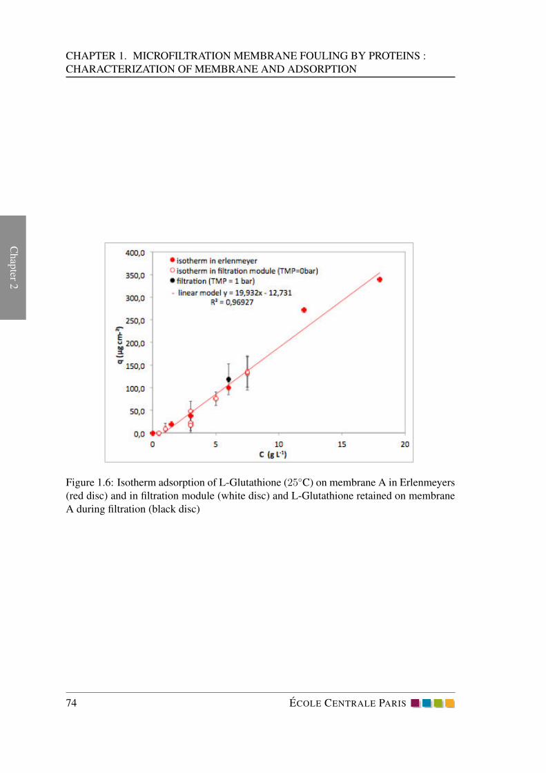
Chap
ter2
CHAPTER 1. MICROFILTRATION MEMBRANE FOULING BY PROTEINS :
CHARACTERIZATION OF MEMBRANE AND ADSORPTION
Figure 1.6: Isotherm adsorption of L-Glutathione (25◦C) on membrane A in Erlenmeyers
(red disc) and in filtration module (white disc) and L-Glutathione retained on membrane
A during filtration (black disc)
74 ECOLE CENTRALE PARIS

3. RESULTS AND DISCUSSION
Chap
ter
2
Figure 1.7: Isotherm adsorption of BSA (25◦C) on membrane A in Erlenmeyers (blue tri-
angle) and in filtration module (white triangle) and BSA retained on membrane A during
filtration (black triangle), compared to literature values obtained during filtration of BSA.
ECOLE CENTRALE PARIS 75

Chap
ter2
CHAPTER 1. MICROFILTRATION MEMBRANE FOULING BY PROTEINS :
CHARACTERIZATION OF MEMBRANE AND ADSORPTION
Figure 1.8: Repeatability tests for membrane A (KOCH) fouling with synthetic solutions
of L-Glutathione (6 gL−1) or BSA (7.5 gL−1) (filtration at 1bar, 0,3m s−1): relative flux
at 20◦C versus time of filtration (min)
At the lowest feed concentration tested (4 g L−1), L-Glutathione can improve the per-
meate flux (Fig. 1.9), suggesting that the membrane is more hydrophilic in the presence
of this protein. On the contrary, BSA already generates 27% of flux decline. At the high-
est concentration (12 g L−1) tested, the flux decline is 18% for L-Glutathione and 51 %for BSA. Mass adsorption of L-Glutathione is 271 µg cm−2 and 135 µg cm−2 for BSA
(Fig. 1.6 and 1.7), but permeability is not impacted by L-Glutathione adsorption, on the
contrary with BSA. L-Glutathione has probably access to a larger surface of adsorption
due to its small size and its penetration into the material, even if it does not generate pore
blocking. The strong link between relative flux J/Jw (measured after 180 min of filtration)
and the mass of protein accumulated on membrane in the case of BSA is demonstrated
in Fig. 1.10. This linear relation could not be generalized: The flux decline was not
the same at all for L-Glutathione even with the same mass of protein accumulated on the
membrane. The relative flux presented here are comparable with those described for BSA
by Hashino et al. (0.65 for BSA at 0.05 g L−1, [95]) and Herrero et al. (0.45 for BSA at
1 gL−1 and 130µg cm−2 ,[99]).
76 ECOLE CENTRALE PARIS

3. RESULTS AND DISCUSSION
Chap
ter
2
Figure 1.9: membrane A (KOCH) fouling with synthetic solutions of L-Glutathione or
BSA at different concentrations (filtration at 1bar, 0,3m s−1): relative permeate flux cor-
rected at 20◦C versus time of filtration (min)
Figure 1.10: membrane A (KOCH) fouling with synthetic solutions of BSA at different
concentrations (filtration at 1bar, 0,3m s−1): relative permeate flux corrected at 20◦C
versus mass of protein adsorbed on membrane.
ECOLE CENTRALE PARIS 77

Chap
ter2
CHAPTER 1. MICROFILTRATION MEMBRANE FOULING BY PROTEINS :
CHARACTERIZATION OF MEMBRANE AND ADSORPTION
Table 1.8: Membrane A (KOCH) filtered with syntethic solutions of L-Glutathione at
different concentrations (filtration 1 bar, 0.3 ms−1): new clean membrane water flux (Jw),
permeate flux during filtration of protein solution (J), water flux with fouled membrane
Jw−f , after 30 min of water rinsing Jw−r and after 30 min of NaOH cleaning Jw−c
J (Lh−1m−2) during the filtration of L-Glutathione, 20◦C
4 gL−1 6 gL−1 (a) 6 gL−1 (b) 6 gL−1 (c) 6 gL−1 (d) 12 gL−1
Jw Lh−1m−2, 20◦C 104.4 158.2 143.5 190.1 142.49 213.7
J (t=0 min)
Lh−1m−2 98.5 157.6 145.2 183.9 137.9 183.9
J (t=180 min)
Lh−1m−2 111.4 148.6 140.1 188.6 136.2 175.1
Jw−f with fouled
membrane Lh−1m−2 - - - 183.9 137.9 -
Jw−r after rinsing 30
min Lh−1m−2 - - - 183.9 137.9 -
Jw−c after cleaning
30 min Lh−1m−2 - - - 183.9 137.9 -
78 ECOLE CENTRALE PARIS

3. RESULTS AND DISCUSSION
Chap
ter
2
Table 1.9: Membrane A (KOCH) filtered with syntethic solutions of BSA at different
concentrations (filtration 1 bar, 0.3 ms−1): new clean membrane water flux (Jw), permeate
flux during filtration of protein solution (J), water flux with fouled membrane Jw−f , after
30 min of water rinsing Jw−r and after 30 min of NaOH cleaning Jw−c
J (Lh−1m−2) during the filtration of BSA, 20◦C
3
gL−16
gL−17.5 gL−1
(a)
7.5 gL−1
(b)
7.5 gL−1
(c)
7.5 gL−1
(d)
10
gL−112
gL−1
Jw Lh−1m−2,
20◦C 169 171.3 183.2 282.7 143.1 114.5 139.4 166.5
J (t=0 min)
Lh−1m−2 162.3 137.9 153.2 229.9 125.4 102.2 110.3 141.4
J (t=180 min)
Lh−1m−2 122.6 106.6 87.5 139.3 81.7 64.5 74.3 74.3
Jw−f with fouled
membrane
Lh−1m−2 - - - - 98.5 76.6 - -
Jw−r after rinsing
30 min Lh−1m−2 - - - - 110.3 81.1 - -
Jw−c after
cleaning 30 min
Lh−1m−2 - - - - 119.9 95.1 - -
Table 1.10: Membrane A (KOCH) filtered with synthetic Solutions L-Glutathione (6
gL−1) and BSA (7.5 gL−1). Filtration at 1bar, 0.3 ms−1. Mass of adsorbed protein on
membrane after fouling (membrane b) and after cleaning (membrane c,d
C
(L-Glutathione) q ±∆q C(BSA) q ±∆q
Membrane (gL−1) µgcm−2 µgcm−2 (gL−1) µgcm−2 µgcm−2
b 6 118.2 34.2 7.5 123.6 14.2
c 6 (cleaned) 0 2.4
7.5
(cleaned) 54.7 8.4
d 6 (cleaned) 0 1.3
7.5
(cleaned) 13.1 3.4
ECOLE CENTRALE PARIS 79

Chap
ter2
CHAPTER 1. MICROFILTRATION MEMBRANE FOULING BY PROTEINS :
CHARACTERIZATION OF MEMBRANE AND ADSORPTION
Figure 1.11: Membrane A (KOCH) fouling with synthetic solution of BSA 7.5 g L−1.
Attribution of flux decline to concentration polarization, reversible, cleanable and irre-
versible fouling.
In order to evaluate the fouling reversibility, a cleaning procedure was carried out.
(See section 2.3). Flux decline with L-Glutathione is very low at 6 g L−1 even if ad-
sorption is measured (118.2 µgcm−2). Rinsing with water and cleaning with NaOH have
no major effect on this parameter even if that quantification of protein before and after
cleaning shows that all accumulated L-Glutathione is removed (Table. 1.8 and 1.10). On
the contrary, with BSA at 7.5 g L−1, after 180 min of filtration, flux decline has reached
43-44%, with the same order of magnitude of protein adsorbed as L-Glutathione (123.6
µ g cm−2) (Table. 1.9 and 1.10). When filtrating water instead of BSA solution with the
fouled membrane, 31-33% of flux decline was observed. The difference of flux decline
corresponds to the impact of polarization of concentration. After water rinsing, reversible
fouling elimination leads to a flux decline of 23-29% .After cleaning with NaOH, 83-84%of the initial water flux is recovered after the elimination of 72% of the adsorbed protein.
Attribution of the flux decline to concentration polarization, reversible fouling, cleanable
fouling (which needs cleaning operations) and irreversible fouling is described in Fig.
1.11.
4 CONCLUSION
In this chapter the structure of two polyethersulfone microfiltration membranes was char-
acterized by scanning electron microscopy, extended bubble point and mercury porosime-
try. For both membranes three layers were identified (active layer, intermediate layer and
mechanical support). The relative thickness of each layer has been identified by a com-
bination of SEM images and ImageJ software. It can be concluded that despite the same
80 ECOLE CENTRALE PARIS

4. CONCLUSION
Chap
ter
2
nature of the membrane’s composition, they presented different properties (pore diameter
of active layer and structure of the intermediate layer). Pore diameters and porosity of
active layer, porosity, pore distribution and active surface of global support were charac-
terized. One of these membranes (PES from KOCH) was used to study the fouling of
a microfiltration module by two organic prodcts: L-Glutathione and Bovine Serum Al-
bumine. Static isotherm experiments showed a linear type adsorption for L-Glutathione
and Langmuir type for BSA. Dynamic isotherm and filtration experiments confirmed the
linear adsorption of L-Glutathione whereas BSA presented lower adsorption than in static
tests, which can be result of steric exclusion of this large protein. Relative flux (J/Jw) was
linearly related to the mass of BSA accumulated on membrane during filtration. Local
adsorption laws could be deduced from membrane structure characterization (membrane
active surface) and adsorption isotherms. Despite comparable values of protein accumu-
lation on the membrane, BSA generate high fouling whereas L-Glutathione no impact of
adsorption on permeability. Reversibility of the fouling was studied for L-Glutathione and
BSA. L-Glutathione could be totally desorbed whereas, cleaning experiments with BSA
showed the presence of polarization concentration, reversible fouling, cleanable fouling
and irreversible fouling.
ECOLE CENTRALE PARIS 81


UPSCALED MODELING OF
MICROLTRATION MEMBRANE FOULING BY
PROTEIN SOLUTIONS : THEORETICAL
STUDY 2
ECOLE CENTRALE PARIS 83

Chap
ter3
CHAPTER 2. UPSCALED MODELING OF MICROLTRATION MEMBRANE
FOULING BY PROTEIN SOLUTIONS : THEORETICAL STUDY
List of symbols
−η related to the bulk fluid
−γ related to the fluid phase
−κ related to the solid phase
−ω related to the membrane active layer
−p related to the membrane porous structure
−s related to the fluid-solid phase
aγκ specific surface area between γ, κ phases, m−1
Aγκ interfacial area between γ − κ, m2
bγ closure variable used to represent the adsorptive source
bγ vector used to represent pγ , m−1
Bγ second order tensor used to represent vγ
cAγ specific concentration of species A in γ phase, kgm−3
cAκ specific concentration of species A in κ phase, kgm−3
〈cAγ〉 superficial average concentration of species A in γ phase, kgm−3
〈cAγ〉γ
intrinsic average concentration of species A in γ phase, kgm−3
cAγ spatial deviation concentration of species A in γ phase, kgm−3
dp characteristic pore size of the membrane, m
Dγ diffusivity of species A in the γ phase (water), m2s
D∗ effective dispersion tensor (Deff +Ddis),m2s
Klan Langmuir adsorption constant for species A, m
K′
lan Langmuir adsorption constant for species A, m3kg
Klin linear adsorption constant for species A, m
Kγ permeability tensor, m2
ℓγ characteristic length scale for γ phase, m
ℓκ characteristic length scale for κ phase, m
ℓmb characteristic length scale of the membrane, m
ℓη macroscopic length scale for η phase (fluid), m
ℓω macroscopic length scale for ω region (active layer), m
ℓp macroscopic length scale for p region (porous structure), m
Lεγ characteristic length scale associated with εγ , m
MA intrinsic molar mass of species A, kgmol−1
nγκ -nκγ , unit normal vector from γ phase to κ phase
nγκ ·wγκ displacement velocity at γ − κ interface
84 ECOLE CENTRALE PARIS

0.
Chap
ter
3
pγ local pressure in the γ phase, Pa
〈pγ〉 superficial average pressure in the γ phase, Pa
〈pγ〉γ
intrinsic average pressure in the γ phase, Pa
pγ spatial deviation of pressure in the γ phase, Pa
sγ vector field used to represent cAγ
u dimensionless vector used to represent the non-local diffusion
vAγ velocity of species A in the γ phase, ms−1
r0 radius of the averaging volume, m
vγ velocity of the γ phase, ms−1
〈vγ〉 superficial velocity of the γ phase, ms−1
〈vγ〉γ
intrinsic velocity of γ phase, ms−1
vγ spatial deviation velocity of the γ phase, ms−1
Greek letters
δ 1− ρAργ
, shrinkage parameter
εγ volume fraction of the γ phase
εκ volume fraction of the κ phase
µγ dynamic viscosity of the fluid (γ) phase, Pa.s
ργ mass density of the γ phase, kgm−3
〈ργ〉 superficial mass density of the γ phase, kgm−3
〈ργ〉γ
intrinsic mass density of the γ phase, kgm−3
ργ spacial deviation of mass density in the γ phase, kgm−3
τ diffA characteristic time of diffusion transport, s
τ convA characteristic time of convection transport, s
τadsA characteristic time of adsorption, s
ECOLE CENTRALE PARIS 85

Chap
ter3
CHAPTER 2. UPSCALED MODELING OF MICROLTRATION MEMBRANE
FOULING BY PROTEIN SOLUTIONS : THEORETICAL STUDY
1 INTRODUCTION
Membrane technology has received considerable interest in separation, purification and
concentration of macromolecules such as proteins in different industrial fields. The prin-
ciple is to separate components of a solution by application a membrane filtration system
with pressure gradient between two sides of the membrane as driving force. The mem-
brane is a porous separator which lets small compounds like water to pass through in the
permeate stream, whereas it retains larger molecules like proteins in the retentate. The
tangential flow devices are less susceptible to fouling than dead-end filtration systems
due to the sweeping effects and high shear rates of the passing flow. However membrane
fouling still exists and leads to a decrease in performance with a loss in solvent perme-
ability and modification in selectivity. Fouling is a common phenomenon observed in all
industrial domains with chemical, environmental, pharmaceutical and biomedical appli-
cations. It is due to chemical (organic or mineral) and biological (biofilm formation) foul-
ing and scale formation. Organic fouling is caused by the accumulation and consequent
deposition of organic materials from the feed water such as humic substances, proteins,
polysaccharides, surfactants etc. onto or within the membrane structure. The problem is
multidisciplinary involving multiphysics (hydrodynamics, mass transport, physical chem-
istry), multiscale (molecules, membrane pores and membrane scales) and time dependent
(microstructure, molecules-surface interactions). In this paper, fouling of microfiltration
membranes by proteins is deepened and an upscaled model associated with protein ad-
sorption to the membrane is proposed.
The main parameters that influence the behaviour of proteins during the filtration are
pH, isoelectric point and ionic strength: the apparent net charge of the protein thus its hy-
dration volume and apparent size, depend on the isoelectric point (IEP) of the molecule
and the pH [62], [272]. It can be concluded from several studies that the protein ad-
sorption is maximum at the IEP where protein is neutral in the aqueous solution[191].
The electrostatic interaction with membrane material depends on the pH (charge den-
sity of the protein and the membrane) and the ionic force of the solution. [62],[156],
[207],[222],[223].The surface charge density and hydrophobicity of the membrane de-
pend also on membrane fouling and evolve with time.
In literature, the reduction of permeability versus time of filtration has been discussed
as a function of different parameters: the intrinsic resistance of the membrane, the com-
position of the feed solution, the fouling mechanisms. Membrane pores are mostly rep-
resented as a package of cylindrical, non-intersecting, homogeneously distributed cap-
illaries with uniform radius assuming (although in most of the cases this assumption is
far from reality) and the solution o be treated is considered a Newtonian fluid with con-
stant properties (density, viscosity) [49],[239]. For instance, concentration polarization
in the diffusion layer caused by steric or electrostatic retention of some solutes adjacent
to the membrane interface can be modeled by the film theory. In this model, there is an
equilibrium between the convective transport from bulk to membrane surface, diffusive
transport from menbrane surface to bulk and diffusive transport from membrane side to
86 ECOLE CENTRALE PARIS

1. INTRODUCTION
Chap
ter
3
the permeate side [156],[271]. In these models the permeate flux is dependent of solute
concentration in bulk, membrane surface and permeate side and also the thickness of the
boundary layer adjacent to the membrane Eq. (10). In this definition, D is the diffusion
coefficient of solutes passing the membrane, vP is the permeate velocity, CP and Cb are
the concentration of solutes at bulk and membrane surface respectively.
Another approach to predict the permeate flux is the series of resistances models based
on the flow of solvent through several transport layers [156],[74],[14]. The series of
resistances consist of progressive additional of membrane resistance due to fouling in
which multiple mechanisms can be involved. The initial membrane resistance Rm de-
pends on the mechanical and chemical properties like membrane thickness, composition,
etc. When the membrane is applied to proteins separation, the accumulation and increase
of proteins near the membrane surface gives an additional resistance due to concentration
polarization Rcp. Above the critical value of the concentration polarization, a gel-like
cake forms on the top layer of the membrane and gives an extra resistance Rc to the
solvent flows the membrane. Moreover the adsorption and/or blockage of solutes at the
membrane interface gives another internal resistance referred as Rin Eq.(2.1). Depending
on the filtration process operational conditions and solvent properties, these models can
include some or all of these additional resistances. In most cases, determination of these
resistance, depends highly on the experimental parameters and remains phenomenologi-
cal.
Permeate flux =∆P
µ(Rmembrane +Rin +RCP +Rcake︸ ︷︷ ︸
Resistance due to fouling
)(2.1)
The models based on the blocking mechanisms predicting the permeate flow are also
used to expiation the evolution of the flow with time[39],[62],[98],[103]. According to
the assumptions taken in these models, membranes are blocked with four different mech-
anisms: complete blocking where it is assumed each particle blocks some pores without
superposition of other particles; standard blocking in which each particle arriving to the
membrane surface deposits into the internal pore walls and decreases the pore volume; in-
termediate blocking where particles can either deposit on other particles, or block directly
some regions of the membrane surface; and finally cake filtration where particles locate
directly on other particles already arrived to the membrane pores. In several studies, a
combination of fouling models is used to evaluate the filtrate flow with time.
These mechanisms have been modeled using empirical or semi-empirical laws, based
on macroscopic measurements. They often use global parameters difficult to link with
physical laws.
The objective of this study is to build a new macroscopic model of membrane fouling
based on local description of the physical problem. This first study will focus on the
modeling of pore constriction generated by protein adsorption.
This is the first study where mass and momentum transport equations flowing through the
membrane are modeled by upscaling methods. The models includes protein adsorption
ECOLE CENTRALE PARIS 87

Chap
ter3
CHAPTER 2. UPSCALED MODELING OF MICROLTRATION MEMBRANE
FOULING BY PROTEIN SOLUTIONS : THEORETICAL STUDY
to the membrane surface and consequent pore constriction is caused by disposed protein
layer to initial membrane structure. However, it should be indicated that we do not invest
in specific protein-membrane electrostatic interactions neither the effects of membrane
surface modification due to adsorption. The model predicts in particular the evolution of
internal structure of the membrane by protein adsorption.
In the following sections, first we provide structural information of the membrane porous
structure (layers with different length scales, mean pore size, permeability and poros-
ity). For this purpose, the membranes have been characterized experimentally. The local
(pore) scale problem accounting for mass and momentum transport equations for fluid
phase with adsorption at solid interface are then given. The upscaled model is elabo-
rated using the volume averaging method in which the development is based on classical
continuum physics. The upscaled model provides the effective permeability and diffu-
sivity which involve both local and structural information of the system. Finally macro-
scopic numerical simulation are run to evaluate the system performance qualitatively.
furthermore, The major challenge in this domain is caused by the minuscule size of the
membrane active layer compared to the thickness of the bulk fluid and membrane porous
structure. To overcome this pure numerical difficulty we replace the membrane active
layer by a dividing surface and then derive jump conditions for mass and momentum
transport equations which contain information of this layer at this new interface. Experi-
mental data of membrane initial structure (porosity) and local protein adsorption laws are
needed to run macroscopic numerical simulations. Eventually, filtration experiments can
be performed to calibrate and/or validate the model.
2 LOCAL DESCRIPTION OF THE MODEL
In this section, the governing mass and momentum equations with corresponding bound-
ary conditions at the pore scale were determined. To have a better vision the membrane
schema with different layers is shown in Fig. 2.1.
In the model we consider two phases: κ refers as solid phase (membrane), and γ referred
as fluid phase (protein solution). When the fluid phase passes through the membrane,
proteins are partly adsorbed on the membrane solid interface leading to complete pore
blocking or reduction of membrane’s pore radius. Although the interactions between
the proteins molecules and solid interface are extremely complex to be characterized
thoroughly, the classic rules are used to model the adsorption which relate in general the
equilibrium protein concentration of the liquid phase to the protein mass adsorbed to the
solid surface. Among these rules, the linear, Langmuir and Freundlich laws are the most
responding. In this work linear and Langmuir adsorption laws are used to model the
adsorption of following model proteins including glutathione and (BSA).
88 ECOLE CENTRALE PARIS

2. LOCAL DESCRIPTION OF THE MODEL
Chap
ter
3
0.3-0.6 μm
15 μm
0.5-10 μm
Porous membrane
Activr layer
Intermediate layer
Mechanical support
Figure 2.1: Microfiltration membrane (supplied by KOCH society) SEM images. 3 layers
have been identified: active layer, intermediate layer and mechanical support.
2.1 HYPOTHESES ASSOCIATED WITH MODEL DEVELOPMENT
As it has been shown in Fig. 2.1, The microfiltration membrane (purchased from KOCH
society) is composed of three different layers: Two first layers are made of polyethersul-
fone (PES) and the mechanical support is composed of polyester (PS). The characteristic
properties of each layer have been obtained. Experiments (capillary flow porometry with
perfluoroethers and mercury) were combined with classical equations of the porous media
(Kozeny-Carman). Let us just recall that Kozeny-Carman is used to describe the porous
structures composed of regular cylinder or sphere solids Eq. (2.2). It is obvious that
the real membrane structure is more complex than regular pores, however it is used to
provide a first approximation in order to make estimations for the simplification of the
ECOLE CENTRALE PARIS 89
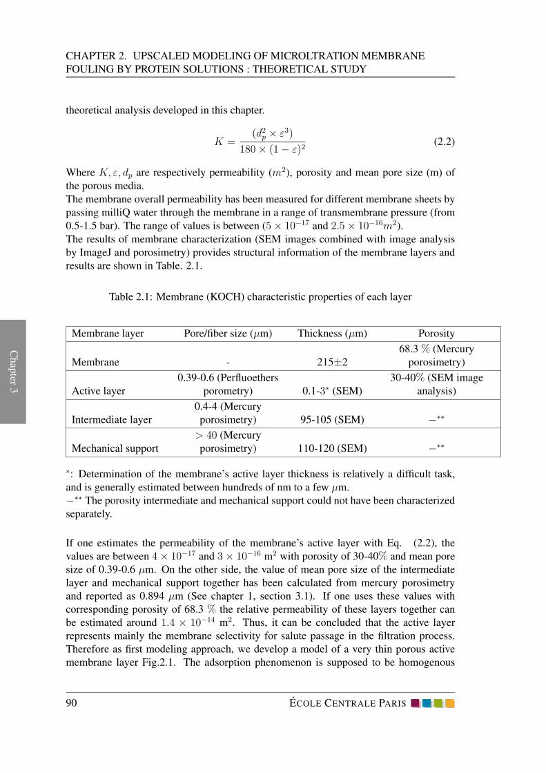
Chap
ter3
CHAPTER 2. UPSCALED MODELING OF MICROLTRATION MEMBRANE
FOULING BY PROTEIN SOLUTIONS : THEORETICAL STUDY
theoretical analysis developed in this chapter.
K =(d2p × ε3)
180× (1− ε)2(2.2)
Where K, ε, dp are respectively permeability (m2), porosity and mean pore size (m) of
the porous media.
The membrane overall permeability has been measured for different membrane sheets by
passing milliQ water through the membrane in a range of transmembrane pressure (from
0.5-1.5 bar). The range of values is between (5× 10⁻¹⁷ and 2.5× 10⁻¹⁶m2).
The results of membrane characterization (SEM images combined with image analysis
by ImageJ and porosimetry) provides structural information of the membrane layers and
results are shown in Table. 2.1.
Table 2.1: Membrane (KOCH) characteristic properties of each layer
Membrane layer Pore/fiber size (µm) Thickness (µm) Porosity
Membrane - 215±2
68.3 % (Mercury
porosimetry)
Active layer
0.39-0.6 (Perfluoethers
porometry) 0.1-3∗ (SEM)
30-40% (SEM image
analysis)
Intermediate layer
0.4-4 (Mercury
porosimetry) 95-105 (SEM) −∗∗
Mechanical support
> 40 (Mercury
porosimetry) 110-120 (SEM) −∗∗
∗: Determination of the membrane’s active layer thickness is relatively a difficult task,
and is generally estimated between hundreds of nm to a few µm.
−∗∗ The porosity intermediate and mechanical support could not have been characterized
separately.
If one estimates the permeability of the membrane’s active layer with Eq. (2.2), the
values are between 4× 10⁻¹⁷ and 3× 10⁻¹⁶ m2 with porosity of 30-40% and mean pore
size of 0.39-0.6 µm. On the other side, the value of mean pore size of the intermediate
layer and mechanical support together has been calculated from mercury porosimetry
and reported as 0.894 µm (See chapter 1, section 3.1). If one uses these values with
corresponding porosity of 68.3 % the relative permeability of these layers together can
be estimated around 1.4 × 10⁻¹⁴ m2. Thus, it can be concluded that the active layer
represents mainly the membrane selectivity for salute passage in the filtration process.
Therefore as first modeling approach, we develop a model of a very thin porous active
membrane layer Fig.2.1. The adsorption phenomenon is supposed to be homogenous
90 ECOLE CENTRALE PARIS

2. LOCAL DESCRIPTION OF THE MODEL
Chap
ter
3
with the membrane active layer. The membrane is a rigid solid phase and is not subject to
dilatation. Adsorption occurs only at the solid interface and there is no diffusion of adsorb
proteins inside the solid phase. Finally, it is assumed that there is no diffusion of adsorb
proteins inside the solid phase. Let us consider first mass and momentum governing
equations at the pore scale and consider the following assumptions for the fluid phase
flowing through the membrane:
• The proteins concentration is of a few g/l (or kg/m3). Taking into account the
intrinsic density of the solvant (about 103 kg/m3 for pure water) and the intrinsic
molar mass of each protein (0.307 kg/mol for L-gluthatione and 66 kg/mol for
BSA), the proteins are diluted in the solution. The specific density of the solution
can then be assumed to be constant: ργ ≈ cst ≈ 103 kg/m3.
• The pressure difference through the membrane is taken to 1 bar = 105 Pa.
• Variations of temperature and pressure during membrane filtration are neglected.
• Viscosity of the solution is assumed to be constant [170].
In the following sections, the local conservation equations (for the fluid phase) are up-
scaled using the volume averaging method.
2.2 PORE SCALE CONSERVATION EQUATIONS
2.2.1 FOR κ-PHASE (SOLID)
For the solid phase, mass conservation can be written
∂ρκ∂t
+∇ · (ργvκ) = 0 (2.3)
The solid phase is assumed to be rigid and still (vκ = 0) and then
∂ρκ∂t
= 0 (2.4)
2.2.2 FOR γ-PHASE (FLUID)
The mass conservation equation for the fluid phase containing diluted species A is given
by∂ργ∂t
+∇ · (ργvγ) = 0 (2.5)
With the assumption that the density ργ of the γ-phase is a constant, we get
∇ · vγ = 0 (2.6)
ECOLE CENTRALE PARIS 91

Chap
ter3
CHAPTER 2. UPSCALED MODELING OF MICROLTRATION MEMBRANE
FOULING BY PROTEIN SOLUTIONS : THEORETICAL STUDY
The momentum equation for the fluid phase is given by the transient Stokes equation.
Indeed, in the present application, the pore Reynolds number has been estimated very
small compared to unity so justifying the use of the Stokes equation instead of the Navier-
Stokes equation. Moreover the gravity body force has been neglected compared to the
pressure gradient (ργg ≈ 104 Pa/m ≪ ∆P/lmb ≈ 5 × 10⁸ Pa/m). This momentum
equation is given by∂ (ργvγ)
∂t= −∇pγ + µγ∇
2vγ (2.7)
The conservation equation of species A in the fluid phase takes the form
∂cAγ
∂t+∇ · (cAγvγ) = ∇ · (Dγ∇cAγ) (2.8)
where Dγ is the diffusion coefficient of species A and cAγ is the specific concentration of
species A. Fick’s law is valid because species A is diluted in the solution.
2.3 PORE SCALE BOUNDARY CONDITIONS
2.3.1 MASS OF SPECIES
Based on the jump condition detailed by [185, 254, 255], the boundary condition at the
fluid-solid interface considering adsorption is
cAγ (vAγ −wγκ) · nγκ =∂cAs
∂tat Aγκ (2.9)
where cAγvAγ = cAγ
(vdAγ + vγ
)= −Dγ∇cAγ + cAγvγ takes into account both diffusion
and convection. At the interface Aγκ, proteins (species A) in fluid phase γ are partly
adsorbed and the adsorption process can be described by different models, usually de-
pending on the bulk protein concentration. As a consequence, Eq. (2.9) can be expressed
as
−Dγ∇cAγ · nγκ + cAγ (vγ −wγκ) · nγκ =∂
∂t[f(cAγ)] at Aγκ (2.10)
where cAs = f(cAγ) and f is the adsorption function for species A, which is an adsorbed
mass per unit area of the interface Aγκ.
2.3.2 TOTAL MASS
Writing, on the fluid side, that the mass flux of solvant (water) through the Aγκ interface
is null and summing with Eq. (2.9) leads to
ργ (vγ −wγκ) · nγκ =∂
∂t[f(cAγ)] at Aγκ (2.11)
92 ECOLE CENTRALE PARIS

2. LOCAL DESCRIPTION OF THE MODEL
Chap
ter
3
Moreover, the intrinsic density of the solid phase is very close to the intrinsic density of
species A (ρκ ≈ ρglu ≈ ρBSA ≈ 1.35 × 10³ kg/m3). From the point of view of mass,
it can be assumed that the solid phase is made of species A only. Therefore, the mass of
species A that is lost by the fluid forms a new part of the solid phase and
ργ (vγ −wγκ) · nγκ ≈ ρA (−wγκ) · nγκ at Aγκ (2.12)
where ρA is the intrisic density of species A.
2.3.3 BOUNDARY CONDITIONS
Combining boundary conditions (2.10), (2.11) and (2.12), the following set of relations
can be obtained
wγκ · nγκ = −1
ρA
∂
∂t[f(cAγ)] at Aγκ (2.13a)
vγ · nγκ = δ (wγκ · nγκ) =
(1
ργ−
1
ρA
)∂
∂t[f(cAγ)] at Aγκ (2.13b)
(vγ −wγκ) · nγκ = (δ − 1) (wγκ · nγκ) =1
ργ
∂
∂t[f(cAγ)] at Aγκ (2.13c)
−Dγ∇cAγ · nγκ = ρA
(cAγ
ργ− 1
)
(wγκ · nγκ) ≈∂
∂t[f(cAγ)] at Aγκ (2.13d)
where δ = 1−ρAργ
≈ −0.35. For the last relation, dilution of speciesA in the solution was
used to say that cAγ ≪ ργ . Finally, and whatever the phenomena in the normal direction,
the no-slip condition for velocity at Aγκ holds: in this case, the component of vγ tangent
to the interface is null because the solid is rigid and still.
2.4 PORE SCALE CHARACTERISTIC TIMES
2.4.1 LITERAL EXPRESSIONS
Estimation of characteristic times of each transport phenomenon (diffusion, convection
and adsorption) can give a better vision of the dominant transport mechanisms and the
possibility to neglect one in comparison to the other one. The characteristic time of
diffusion of species A in a pore is given by
DAB τdiffA
ℓγ2 = 1 =⇒ τ diffA =
ℓγ2
Dγ
(2.14)
where lγ is a typical pore size.
ECOLE CENTRALE PARIS 93

Chap
ter3
CHAPTER 2. UPSCALED MODELING OF MICROLTRATION MEMBRANE
FOULING BY PROTEIN SOLUTIONS : THEORETICAL STUDY
The characteristic time of convection of species A in a pore can be deduced from Eq.
(2.8) ∣∣∣∣
∂cAγ
∂t
∣∣∣∣= O (|vγ.∇cAγ|) =⇒ τ convA =
ℓγvγ
(2.15)
The characteristic time of adsorption depends on the adsorption law for each protein.
It can be deduced that
−DAB∇cAγ · nγκ = O
(∂
∂t[f(cAγ)]
)
at Aγκ (2.16)
For a linear law, flin(cAγ) = KlincAγ and thus
τadslin =ℓγDγ
Klin (2.17)
For a Langmuir law, flan(cAγ) =KlancAγ
1 +K ′lancAγ
and thus
τadslan =ℓγDγ
Klan
1 +K ′lancAγ
(2.18)
Here we remind that in several experimental studies, the Langmuir adsorption
isotherms is expressed as follows:
q =qmaxKACA
1 +KACA
(2.19)
Where q is the species concentration at interface, qmax is the maximum sorption ca-
pacity and KA is the half saturation constant (See Chapter 1).
2.4.2 APPLICATION TO L-GLUTHATIONE AND BSA
For the membrane used in this work the the mean pore size bass been measured ℓγ ∼0.6 ≈ µm. The pore scale diffusion coefficients of L-glutathione and BSA are calculated
from the Stokes-Einstein equatio, Dγ(glut) = 5.40×10⁻¹⁰ m2/s and Dγ(BSA) = 9.04×10⁻¹¹ m2/s. Hence, the characteristic diffusion times for both protein can be estimated
as τ diffglu ≈ 7× 10⁻⁴ s and τ diffBSA ≈ 3× 10⁻³ s.
The average velocity in the pores is estimated to 10−5 m/s from experiments, leading to
τ convA ≈ 6 × 10⁻² s. Let us note that the characteristic times of diffusion and convection
have comparable order of magnitude and therefore both diffusion and convection have to
be accounted for in the analysis.
For L-glutathione,a linear adsorption isotherm was found experimentally whereas and
for BSA, a langmuir isotherm has been observed. The adsorption characteristic time
varies then between 10−4 and 10−3 s for protein solutions, which is of the same order of
magnitude than the other phenomena.
94 ECOLE CENTRALE PARIS

3. UPSCALING
Chap
ter
3
3 UPSCALING
Let us consider a schematic membrane and an associated Representative Elementary Vol-
ume (REV) where the different scales of the system are described (Fig. 2.2).
Figure 2.2: Representative Elementary Volume with fluid and solid phases and unit nor-
mal vectors
Let us recall that the superficial average of any function associated with the γ-phase is
defined by [255]
〈Ψγ〉 =1
V
∫
Vγ(t)
ΨγdV (2.20)
while the intrinsic average takes the form
〈Ψγ〉γ =
1
Vγ(t)
∫
Vγ(t)
ΨγdV (2.21)
These two averages being related by
〈Ψγ〉 = εγ 〈Ψγ〉γ
(2.22)
ECOLE CENTRALE PARIS 95
Chap
ter3
CHAPTER 2. UPSCALED MODELING OF MICROLTRATION MEMBRANE
FOULING BY PROTEIN SOLUTIONS : THEORETICAL STUDY
Note that these averages make sense if the different scales of the system satisfy the scale
separation given by ℓγ ≪ r0 ≪ ℓmb. The upscaling procedure for the derivation of
average governing transport equations requires the three following theorems (Howes and
Whitaker, 1985)
〈∇Ψγ〉 = ∇〈Ψγ〉+1
V
∫
Aγκ
nγκΨγdS (2.23)
〈∇ ·Ψγ〉 = ∇ · 〈Ψγ〉+1
V
∫
Aγκ
nγκ ·ΨγdS (2.24)
⟨∂Ψγ
∂t
⟩
=∂ 〈Ψγ〉
∂t−
1
V
∫
Aγκ
(nγκ ·wγκ)ΨγdS (2.25)
where wγκ is the interfacial velocity of Aγκ.
3.1 AVERAGE MASS CONSERVATION
3.1.1 FOR κ-PHASE (SOLID)
Taking the average of the mass conservation equation in the κ-phase, Eq. (2.4), gives
∂ (εκ 〈ρκ〉κ)
∂t−
1
V
∫
Aγκ
(nκγ ·wγκ) ρκdA = 0 (2.26)
The solid density is a constant and then
∂εγ∂t
= −∂εκ∂t
=1
V
∫
Aγκ
nγκ ·wγκdA (2.27)
where we used the fact that εγ + εκ = 1.
3.1.2 FOR γ-PHASE (FLUID)
Applying the averaging operator to the mass conservation equation in the γ-phase, Eq.
(2.6) leads to
∇ · 〈vγ〉 = −1
V
∫
Aγκ
nγκ · vγdA (2.28)
3.2 AVERAGE MOMENTUM CONSERVATION
The average of Eq. (2.7) gives
⟨∂ (ργvγ)
∂t
⟩
= −〈∇pγ〉+⟨µγ∇
2vγ
⟩(2.29)
96 ECOLE CENTRALE PARIS

3. UPSCALING
Chap
ter
3
Folllowing Bousquet-Melou et al., [29], we first develop each term of the above equation
before providing the full averaged momentum equation.
3.2.1 ACCUMULATION TERM
Since the density has been assumed to be constant, the averaged accumulation term takes
the form⟨∂ (ργvγ)
∂t
⟩
=∂ (ργεγ 〈vγ〉
γ)
∂t−
1
V
∫
Aγκ
(nγκ ·wγκ)ργvγdA (2.30)
or⟨∂ (ργvγ)
∂t
⟩
= εγργ∂ 〈vγ〉
γ
∂t+∂εγ∂t
ργ 〈vγ〉γ −
1
V
∫
Aγκ
(nγκ ·wγκ)ργvγdA (2.31)
3.2.2 PRESSURE TERM
The average form of the pressure term is
〈∇pγ〉 = ∇ (εγ 〈pγ〉γ) +
1
V
∫
Aγκ
nγκpγdA (2.32)
Using the Gray decomposition and a length scale constraint to take 〈pγ〉γ
out of the inte-
gral, it can be written
1
V
∫
Aγκ
nγκpγdA = − (∇εγ) 〈pγ〉γ +
1
V
∫
Aγκ
nγκpγdA (2.33)
and therefore the average pressure term is given by
−〈∇pγ〉 = −εγ∇〈pγ〉γ −
1
V
∫
Aγκ
nγκpγdA (2.34)
3.2.3 DIFFUSION TERM
The averaged viscous term, assuming constant liquid viscosity, is given by
⟨µγ∇
2vγ
⟩= µγ∇
2(εγ 〈vγ〉γ) +
1
V
∫
Aγκ
nγκ · (µγ∇vγ)dA
+ µγ∇ ·
(
1
V
∫
Aγκ
nγκvγdA
)
(2.35)
If there was no-slip and no-penetration at Aγκ, the last area integral would disappear.
However, for now, the interfacial velocity is non zero. Using the Gray decomposition of
ECOLE CENTRALE PARIS 97

Chap
ter3
CHAPTER 2. UPSCALED MODELING OF MICROLTRATION MEMBRANE
FOULING BY PROTEIN SOLUTIONS : THEORETICAL STUDY
velocity in the last term of Eq. (2.35) provides
1
V
∫
Aγκ
nγκ · (µγ∇vγ)dA
≈ −µγ (∇εγ) · (∇〈vγ〉γ) +
1
V
∫
Aγκ
nγκ · (µγ∇vγ)dA (2.36)
and then
⟨µγ∇
2vγ
⟩= µγ∇
2(εγ 〈vγ〉γ)− µγ (∇εγ) · (∇〈vγ〉
γ)
+1
V
∫
Aγκ
nγκ · (µγ∇vγ)dA+ µγ∇ ·
(
1
V
∫
Aγκ
nγκvγdA
)
(2.37)
Finally, writing
µγ∇2(εγ 〈vγ〉
γ) = εγµγ∇2 〈vγ〉
γ + µγ (∇εγ) · (∇〈vγ〉γ) (2.38)
+ µγ∇ · [(∇εγ) 〈vγ〉γ]
we get
⟨µγ∇
2vγ
⟩= εγµγ∇
2 〈vγ〉γ + µγ∇ · [(∇εγ) 〈vγ〉
γ] +1
V
∫
Aγκ
nγκ · (µγ∇vγ)dA
+µγ∇ ·
(
1
V
∫
Aγκ
nγκvγdA
)
(2.39)
3.2.4 NON-CLOSED EQUATION
Finally, combination of Eqs. (2.31), (2.34), (2.39) leads to the non-closed average mo-
mentum equation for the fluid flow through the porous membrane
εγργ∂ 〈vγ〉
γ
∂t+ ργ 〈vγ〉
γ ∂εγ∂t
= −εγ∇〈pγ〉γ + εγµγ∇
2 〈vγ〉γ + µγ∇ · [(∇εγ) 〈vγ〉
γ]
+1
V
∫
Aγκ
nγκ · (−Ipγ + µγ∇vγ)dA+ µγ∇ ·
(
1
V
∫
Aγκ
nγκvγdA
)
+1
V
∫
Aγκ
(nγκ ·wγκ)ργvγdA (2.40)
The originality of the non-closed averaged form of momentum transport is that it ex-
plicitly involves the time evolution of the membrane porosity due to adsorption. This
additional term depends on the adsorption law of the protein.
98 ECOLE CENTRALE PARIS

3. UPSCALING
Chap
ter
3
3.3 AVERAGE SPECIES CONSERVATION
The average of Eq. (2.8) is the sum of the averaged of each terms of the pore scale species
conservation equation
⟨∂cAγ
∂t
⟩
+ 〈∇ · (cAγvγ)〉 = 〈∇ · (Dγ∇cAγ)〉 (2.41)
As previously, each term of Eq. (2.41) is averaged separately.
3.3.1 ACCUMULATION TERM
Using the general transport theorem, the accumulation term of Eq. (2.41) becomes
⟨∂cAγ
∂t
⟩
= εγ∂ 〈cAγ〉
γ
∂t−
1
V
∫
Aγκ
(nγκ ·wγκ)cAγdA (2.42)
after using Gray decomposition on concentration and Eq. (2.27).
3.3.2 CONVECTION TERM
Using the spatial averaging theorem, the convective term of Eq. (2.41) becomes
〈∇ · (cAγvγ)〉 = ∇ · 〈cAγvγ〉+1
V
∫
Aγκ
(nγκ · vγ) cAγdA (2.43)
Following the same steps as for the average momentum transport equation, we obtain the
final expression of the convection term
〈∇ · (cAγvγ)〉 = εγ 〈vγ〉γ · ∇ 〈cAγ〉
γ +∇ · 〈cAγvγ〉
+1
V
∫
Aγκ
(nγκ · vγ) cAγdA (2.44)
3.3.3 DIFFUSION TERM
For conciseness, all the details regarding the classical averaging of the diffusion term are
not repeated here. For more details, the reader is invited to consult the reference [255].
The diffusion term can therefore be written
〈∇ · (Dγ∇cAγ)〉 = εγ∇ · (Dγ∇〈cAγ〉γ) + (∇εγ) · (Dγ∇〈cAγ〉
γ)
+∇ ·
(
Dγ
V
∫
Aγκ
nγκcAγdA
)
−1
V
∫
Aγκ
nγκ · (−Dγ∇cAγ) dA (2.45)
ECOLE CENTRALE PARIS 99

Chap
ter3
CHAPTER 2. UPSCALED MODELING OF MICROLTRATION MEMBRANE
FOULING BY PROTEIN SOLUTIONS : THEORETICAL STUDY
3.3.4 NON-CLOSED EQUATION
Finally, the non-closed species conservation takes the form
∂ 〈cAγ〉γ
∂t+ 〈vγ〉
γ · ∇ 〈cAγ〉γ = ∇ · (Dγ∇〈cAγ〉
γ)
+ε−1γ ∇ ·
(
Dγ
V
∫
Aγκ
nγκcAγdA
)
+ ε−1γ (∇εγ) · (Dγ∇〈cAγ〉
γ)
−ε−1γ ∇ · 〈vγ cAγ〉 −
1
Vγ
∫
Aγκ
nγκ · [−Dγ∇cAγ + (vγ −wγκ) cAγ] dA
(2.46)
The set of non-closed averaged conservation equations obtained involve numerous devia-
tion terms. In the next section, additional considerations and assumptions are formulated
to simplify these equations in order to derive associated closure problems whose solutions
are related to the effective transport properties of the closed system.
4 SIMPLIFICATIONS
4.1 SMALL PORE SCALE GROWTH VELOCITY
According to [29], the processes involving a change of the porous microstructure due to
phase change or chemical / biological reactions, can generally be modeled considering
that the growth velocity of the solid phase is small compared to the average fluid velocity
in the direction normal to the interface
|wγκ · nγκ| ≪ |〈vγ〉γ · nγκ| at Aγκ (2.47)
The authors were interested in dendritic solidification but this observation is still relevant
in the present context of adsorption.
4.2 SIMPLIFIED FORM OF PORE SCALE BOUNDARY CONDITIONS
Eq. (2.13b) becomes
vγ · nγκ = δ (wγκ · nγκ)− 〈vγ〉γ · nγκ at Aγκ (2.48)
and then, with Eq. (2.47) and |δ| < 1,
vγ · nγκ ≈ −〈vγ〉γ · nγκ at Aγκ (2.49)
100 ECOLE CENTRALE PARIS

4. SIMPLIFICATIONS
Chap
ter
3
This is a non-penetration condition. Associated to the no-slip condition, it gives
vγ ≈ 0 at Aγκ (2.50)
It must be kept in mind that |wγκ · nγκ| is small compared to |〈vγ〉γ · nγκ| but not null
(otherwise, there would not be any adsorption).
Taking into account these considerations, the pore scale relations (2.13a), (2.13b), (2.13c)
and (2.13d) leads to
wγκ · nγκ = −1
ρA
∂
∂t[f(cAγ)] at Aγκ (2.51a)
vγ ≈ 0 at Aγκ (2.51b)
(vγ −wγκ) · nγκ =1
ργ
∂
∂t[f(cAγ)] at Aγκ (2.51c)
−Dγ∇cAγ · nγκ =∂
∂t[f(cAγ)] at Aγκ (2.51d)
In this situation, growth velocity has a negligible influence on hydrodynamics and species
A transport, but is important in the evolution of the porosity εγ with time (and is even the
only source of evolution).
4.3 SIMPLIFIED FORM OF AVERAGE MASS CONSERVATION
4.3.1 FOR κ-PHASE (SOLID)
The growth velocity is known by the relation (2.51a) and the evolution of porosity can
then be expressed as a function of species A concentration. Eq. (2.27) becomes
∂εγ∂t
=1
V
∫
Aγκ
(
−1
ρA
∂
∂t[f(cAγ)]
)
dA (2.52)
and consequently, with the surface transport theorem [228],
∂εγ∂t
=∂
∂t
(
1
V
∫
Aγκ
−1
ρAf(cAγ)dA
)
(2.53)
where the displacement of the surface has been assumed to be mainly normal and where
the effects of curvature of the surface have been neglected. A Taylor expansion at first
ECOLE CENTRALE PARIS 101

Chap
ter3
CHAPTER 2. UPSCALED MODELING OF MICROLTRATION MEMBRANE
FOULING BY PROTEIN SOLUTIONS : THEORETICAL STUDY
order for f shows that
f(cAγ) = f(〈cAγ〉γ + cAγ) = f(〈cAγ〉
γ) + cAγf′(〈cAγ〉
γ) + · · · ≈ f(〈cAγ〉γ)
(2.54)
where cAγ has been assumed to be small compared to 〈cAγ〉γ, as in usual diffusion prob-
lems (see [255], section 1.4.2). It is indeed sufficient to neglect the terms of order higher
than one for the adsorption laws considered here (linear and Langmuir).
Using the specific surface area aγκ(x, t) = Aγκ(x, t)/V , Eq. (2.53) becomes
∂εγ∂t
= −1
ρA
∂
∂t[aγκf(〈cAγ〉
γ)] (2.55)
and therefore, by integration between time t and time 0
εγ(x, t) = εγ0 −
1
ρAaγκ(x, t)f(〈cAγ〉
γ)(x, t) (2.56)
where εγ0 is the porosity at initial time. Indeed, the membrane has been assumed to be
unfouled at initial time (〈cAγ〉γ (x, 0) = 0), and f(0) = 0 for any adsorption law. The
function f is positive and then, as expected, the porosity εγ is at any time smaller than
initial porosity.
In the next sections, it would be simpler if the relative gradients of porosity ∇εγ could
be neglected. To assess if this assumption is correct, an expression or an equation of
evolution for aγκ is needed, in order to estimate its gradient. Starting with
aγκ ∼1
ℓγ∼ (Vγ)
−1/3(2.57)
and reminding that εγ =VγV
, the following equation is proposed for the specific surface
area
aγκaγκ0
=
(εγεγ0
)−1/3
(2.58)
Consequently
∇aγκaγκ
= −1
3
(∇εγεγ
)
(2.59)
102 ECOLE CENTRALE PARIS

4. SIMPLIFICATIONS
Chap
ter
3
and then Eq. (2.56) gives
∇εγεγ
=
−1
ρA
(aγκεγ
)
∇ (f(〈cAγ〉γ))
1−1
3ρA
(aγκεγ
)
f(〈cAγ〉γ)
(2.60)
As presented in Eq. (2.60), the expression of the porosity gradient depends only on the
adsorption rate which is function of protein concentration. Even though it is clear that the
porosity gradient is not null, it can be estimated that its variations at the membrane scale
is negligible. Therefore one can estimate Eq. (2.60) with the following expression
∇εγεγ
≈1
Lεγ
(2.61)
Lεγ is a macroscopic length scale associated to the porosity at the membrane-scale. Us-
ing this length-scale constraint, we can neglect the porosity gradients in the rest of the
analysis.
4.3.2 FOR γ-PHASE (FLUID)
Mass conservation in the fluid, Eq. (2.28), along with the boundary condition (2.51b),
changes into
∇ · 〈vγ〉 = 0 (2.62)
and thus, with negligible gradients of porosity
∇ · 〈vγ〉γ = 0 (2.63)
4.4 SIMPLIFIED FORM OF AVERAGE MOMENTUM CONSERVATION
With the relation (2.51b) and divided by εγ , Eq. (2.40) becomes
ργ∂ 〈vγ〉
γ
∂t+ ργ 〈vγ〉
γ ε−1γ
∂εγ∂t
= −∇〈pγ〉γ + µγ∇
2 〈vγ〉γ +
1
Vγ
∫
Aγκ
nγκ · (−Ipγ + µγ∇vγ)dA
(2.64)
where gradients of porosity have been neglected again.
ECOLE CENTRALE PARIS 103
Chap
ter3
CHAPTER 2. UPSCALED MODELING OF MICROLTRATION MEMBRANE
FOULING BY PROTEIN SOLUTIONS : THEORETICAL STUDY
4.5 SIMPLIFIED FORM OF AVERAGE SPECIES CONSERVATION
With the relation (2.51b) and neglecting porosity gradients, Eq. (2.46) gives
∂ 〈cAγ〉γ
∂t+ ε−1
γ aγκ∂
∂t[f(〈cAγ〉
γ)] + f(〈cAγ〉γ)ε−1
γ
∂aγκ∂t
+ 〈vγ〉γ · ∇ 〈cAγ〉
γ
= ∇ · (Dγ∇〈cAγ〉γ) + ε−1
γ ∇ ·
(
Dγ
V
∫
Aγκ
nγκcAγdA
)
− ε−1γ ∇ · 〈vγ cAγ〉 (2.65)
where (2.51c) and (2.51d) were used to obtain
|nγκ · (vγ −wγκ) cAγ|
|nγκ · (−Dγ∇cAγ)|= O
(cAγ
ργ
)
≪ 1 (2.66)
(2.67)
−1
Vγ
∫
Aγκ
nγκ · (−Dγ∇cAγ) dA
= −ε−1γ aγκ
∂
∂t[f(〈cAγ〉
γ)]− ε−1γ f(〈cAγ〉
γ)∂aγκ∂t
(2.68)
in the same manner as before.
4.6 SIMPLIFIED SYSTEM OF EQUATIONS
Finally, the simplified average transport equations are Eqs. (2.56), (2.58), (2.63), (2.64)
and (2.65)
∇ · 〈vγ〉γ = 0 (2.69a)
ργ∂ 〈vγ〉
γ
∂t+ ργ 〈vγ〉
γ ε−1γ
∂εγ∂t
(2.69b)
= −∇〈pγ〉γ + µγ∇
2 〈vγ〉γ +
1
Vγ
∫
Aγκ
nγκ · (−Ipγ + µγ∇vγ)dA
[1 + ε−1
γ aγκf′(〈cAγ〉
γ)] ∂ 〈cAγ〉
γ
∂t+ ε−1
γ f(〈cAγ〉γ)∂aγκ∂t
+ 〈vγ〉γ · ∇ 〈cAγ〉
γ
= ∇ · (Dγ∇〈cAγ〉γ) + ε−1
γ ∇ ·
(
Dγ
V
∫
Aγκ
nγκcAγdA
)
− ε−1γ ∇ · 〈vγ cAγ〉 (2.69c)
104 ECOLE CENTRALE PARIS

5. DEVIATIONS AND CLOSURE PROBLEMS
Chap
ter
3
εγ = εγ0 −
1
ρAaγκf(〈cAγ〉
γ) (2.69d)
aγκ = aγκ0
(εγεγ0
)−1/3
(2.69e)
To conclude this section, it is worth mentioning that, at this stage, the non closed
hydrodynamics problem explicitly involves the time evolution of porosity. Rigorously,
that is to say that both the closed momentum equation and the solution of the associated
closure problem for the determination of the permeability depend on this evolution. For
the closed momentum equation, this is not a difficulty since this additional term explicitly
depends on the adsorption rate. The solution of the closure problem is more complicated
if the time evolution of porosity is treated as a source term. This remains a challenge
which is out of reach of the present study. In the following, this dependency will be
neglected and the classical closure problem will be considered for the determination of
the permeability.
Moreover, the evolution of the species A concentration is described by a convection-
diffusion equation with a modified accumulation term due to adsorption. For the same
reason af for the momentum equation, the contribution of the time evolution of specific
surface area will be discarded in the closure problem.
5 DEVIATIONS AND CLOSURE PROBLEMS
The objective of this section is to derive the associated closure problems. Only the main
steps are recalled here in order to make the coupling with species transport more under-
standable.
5.1 CLOSURE PROBLEM FOR MOMENTUM CONSERVATION
Since the source term related to the time evolution of the porosity has been discarded
from the closure problem for momentum, it reduces to a classical form. The deviation
problem for momentum is given by [255]
0 = −∇pγ + µγ∇2vγ −
1
Vγ
∫
Aγκ
nγκ · (−Ipγ + µγ∇vγ)dA (2.70a)
∇ · vγ = 0 (2.70b)
vγ = −〈vγ〉γ
︸ ︷︷ ︸
source
at Aγκ (2.70c)
pγ(r + li) = pγ(r), vγ(r + li) = vγ(r), i = 1, 2, 3 (2.70d)
〈vγ〉γ = 0 (2.70e)
ECOLE CENTRALE PARIS 105

Chap
ter3
CHAPTER 2. UPSCALED MODELING OF MICROLTRATION MEMBRANE
FOULING BY PROTEIN SOLUTIONS : THEORETICAL STUDY
where the relevance of periodicity conditions for both pressure and velocity fields has
been frequently discussed [255]. It is worth noticing that periodicity conditions only
makes sense for constant or periodic sources. In the above deviation problem, 〈vγ〉γ
is a
constant since the length-scale constraint
r0 ≪ ℓmb (2.71)
is satisfied, and it is then a source term for deviations. The characteristic length of the
representative unit cell will always be of the order of r0 or smaller.
The nature of the deviation momentum problem suggests that the deviation solutions can
be written under the form
vγ = Bγ · 〈vγ〉γ
(2.72a)
pγ = µγbγ · 〈vγ〉γ
(2.72b)
Therefore, the associated closure problem for the variables Bγ and bγ is defined by
0 = −∇bγ +∇2Bγ −1
Vγ
∫
Aγκ
nγκ · (−Ibγ +∇Bγ)dA (2.73a)
∇Bγ = 0 (2.73b)
Bγ = −I at Aγκ (2.73c)
bγ(r + li) = bγ(r), Bγ(r + li) = Bγ(r), i = 1, 2, 3 (2.73d)
〈Bγ〉γ = 0 (2.73e)
The permeability tenser Kγ is defined as
1
Vγ
∫
Aγκ
nγκ · (−Ibγ +∇Bγ)dA = −εγK−1γ (2.74)
The solution of Eq. (2.73) is the classical solution of the Stokes closure problem and is
explained thoroughly in [255].
5.2 CLOSURE PROBLEM FOR SPECIES CONSERVATION
5.2.1 DEVIATION PROBLEM
The objective of this section is to determine the deviation of speciesA concentration, cAγ ,
as a function of average quantities, in order to obtain a closed form of the average species
concentration equation. To get the governing differential equation for cAγ , the non-closed
106 ECOLE CENTRALE PARIS

5. DEVIATIONS AND CLOSURE PROBLEMS
Chap
ter
3
average conservation equation Eq. (2.69c)
∂ 〈cAγ〉γ
∂t+ ε−1
γ aγκ∂
∂t[f(〈cAγ〉
γ)] + ε−1γ f(〈cAγ〉
γ)∂aγκ∂t
+ 〈vγ〉γ · ∇ 〈cAγ〉
γ
= ∇ · (Dγ∇〈cAγ〉γ) + ε−1
γ ∇ ·
(
Dγ
V
∫
Aγκ
nγκcAγdA
)
− ε−1γ ∇ · 〈vγ cAγ〉
(2.75)
is substracted from the pore scale one Eq. (2.8)
∂cAγ
∂t+∇ · (cAγvγ) = ∇ · (Dγ∇cAγ) (2.76)
Thus
∂cAγ
∂t︸ ︷︷ ︸
Accumulation
− ε−1γ aγκ
∂
∂t[f(〈cAγ〉
γ)]︸ ︷︷ ︸
Adsorptive source
+vγ · ∇cAγ︸ ︷︷ ︸
Convection
+ vγ · ∇ 〈cAγ〉γ
︸ ︷︷ ︸
Convective source
= ∇ · (Dγ∇cAγ)︸ ︷︷ ︸
Diffusion
− ε−1γ ∇ ·
(
Dγ
V
∫
Aγκ
nγκcAγdA
)
︸ ︷︷ ︸
Non-local diffusion
+ ε−1γ ∇ · 〈vγ cAγ〉︸ ︷︷ ︸
Non-local convection
(2.77)
where the term arising from the evolution with time of the specific surface area has been
discarded, as previously discussed. The thorough procedure of the simplification of this
deviation equation, detailed in Appendix A, gives
− ε−1γ aγκ
∂
∂t[f(〈cAγ〉
γ)]︸ ︷︷ ︸
Adsorptive source
+vγ · ∇cAγ︸ ︷︷ ︸
Convection
+ vγ · ∇ 〈cAγ〉γ
︸ ︷︷ ︸
Convective source
= ∇ · (Dγ∇cAγ)︸ ︷︷ ︸
Diffusion
(2.78)
5.2.2 BOUNDARY CONDITIONS
Reminding pore scale boundary condition (2.13d)
−Dγ∇cAγ · nγκ =∂
∂t[f(cAγ)] on Aγe (2.79)
ECOLE CENTRALE PARIS 107

Chap
ter3
CHAPTER 2. UPSCALED MODELING OF MICROLTRATION MEMBRANE
FOULING BY PROTEIN SOLUTIONS : THEORETICAL STUDY
the initial and boundary conditions for the deviation problem are
−Dγ∇cAγ · nγκ = Dγ∇〈cAγ〉γ · nγκ
︸ ︷︷ ︸
Diffusion source
+∂
∂t[f(〈cAγ〉
γ)]︸ ︷︷ ︸
Adsorptive source
at Aγκ
(2.80a)
cAγ = F(r, t) on Aγe (2.80b)
cAγ = G(r) at t = 0 (2.80c)
5.2.3 CLOSURE PROBLEM
There is not interest in solving cAγ in the whole macroscopic region because the numer-
ical cost would be about the same as for the pore scale problem. Instead, cAγ will be
determined in different regions that are representative of the structure of the original one.
Given that cAγ is dominated by the small length scale, the boundary condition imposed
on entrances and exits in (A.13b) can influence the cAγ-field only in a very thin region
near the entrances and exits of the macroscopic system. Therefore, each representative
region will be modeled as a periodic unit cell, where boundary conditions at Aγe have
been replaced by periodic boundary conditions.
This leads to the closure problem given by
− ε−1γ aγκ
∂
∂t[f(〈cAγ〉
γ)]︸ ︷︷ ︸
Adsorptive source
+vγ · ∇cAγ︸ ︷︷ ︸
Convection
+ vγ · ∇ 〈cAγ〉γ
︸ ︷︷ ︸
Convective source
= ∇ · (Dγ∇cAγ)︸ ︷︷ ︸
Diffusion
(2.81a)
−Dγ∇cAγ · nγκ = Dγ∇〈cAγ〉γ · nγκ
︸ ︷︷ ︸
Diffusion source
+∂
∂t[f(〈cAγ〉
γ)]︸ ︷︷ ︸
Adsorptive source
at Aγκ
(2.81b)
cAγ(r + li) = cAγ(r) i = 1, 2, 3 (2.81c)
It is important to notice that at the scale of a unit cell (ℓγ), the macroscopic terms can be
treated as constants and equal to their value at the center x of the unit cell. Furthermore,
the solution cAγ of this problem is not unique since any additive constant can be added to
a solution to form another solution. Nevretheless, this constant does not pass through the
integral filter of Eq. (2.69c) because the representative medium is periodic. Any solution
will then lead to the same result for the closed average species conservation.
5.2.4 CLOSURE VARIABLES
According to the closure problem, the macroscopic source terms are ∇〈cAγ〉γ
and∂
∂t[f(〈cAγ〉
γ)]. cAγ is then searched under the form of a first order development with
108 ECOLE CENTRALE PARIS

6. CLOSED FORM OF THE MACROSCOPIC MODEL
Chap
ter
3
respect to these terms
cAγ = sγ · ∇ 〈cAγ〉γ + bγ
∂
∂t[f(〈cAγ〉
γ)] (2.82)
The constant (zeroth order of the development) has been here taken equal to zero, since it
does not pass through the integral filter of Eq. (2.69c), as seen before.
Introducting this expression into Eqs. (2.81) and treating source terms as constants in the
unit cell, the closure variables sγ and bγ verify the following uncoupled systems
Problem I
vγ · ∇sγ + vγ = ∇ · (Dγ∇sγ) (2.83a)
B.C.: −nγκ · Dγ∇sγ = Dγnγκ at Aγκ (2.83b)
Periodicity: sγ(r+ li) = sγ(r) (2.83c)
Problem II
−ε−1γ aγκ + vγ · ∇bγ = ∇ · (Dγ∇bγ) (2.84a)
B.C.: −nγκ · Dγ∇bγ = 1 at Aγκ (2.84b)
Periodicity: bγ(r+ li) = bγ(r) (2.84c)
6 CLOSED FORM OF THE MACROSCOPIC MODEL
6.1 CLOSED AVERAGE MASS CONSERVATION
Eq. (2.69a) was already closed
∇ · 〈vγ〉γ = 0 (2.85)
6.2 CLOSED AVERAGE MOMENTUM CONSERVATION
In order to obtain a closed form of the macroscopic momentum conservation with adsorp-
tion, velocity and pressure deviations given by Eqs. (2.72a) and (2.72b) are introduced
into Eq. (2.69c)
ργ∂ 〈vγ〉
γ
∂t+ ργ 〈vγ〉
γ ε−1γ
∂εγ∂t
= −∇〈pγ〉γ + µγ∇
2 〈vγ〉γ
+ µγ
[
1
Vγ
∫
Aγκ
nγκ · (−Ibγ +∇Bγ)dA
]
· 〈vγ〉γ
(2.86)
ECOLE CENTRALE PARIS 109

Chap
ter3
CHAPTER 2. UPSCALED MODELING OF MICROLTRATION MEMBRANE
FOULING BY PROTEIN SOLUTIONS : THEORETICAL STUDY
which can be written under the more compact form
ργ∂ 〈vγ〉
γ
∂t+ ργ 〈vγ〉
γ ε−1γ
∂εγ∂t
= −∇〈pγ〉γ + µγ∇
2 〈vγ〉γ − µγK
−1γ · εγ 〈vγ〉
γ
(2.87)
It should be noticed that Eq. (2.87) represents an improvement in the derivation of the
upscaled momentum transport equation for porous media for which microstructure can
be time dependent. However, it is important to clearly identify its limitations. Indeed,
Eq. (2.87) has been derived first by assuming a small interface velocity and secondly by
neglecting in the closure problem the source term related to the evolution with time of the
structure. The authors are conscious that deeper analysis is needed in order to deal with
this complexity.
6.3 CLOSED AVERAGE SPECIES CONSERVATION
In order to obtain a closed form of the macroscopic species conservation with adsorption,
concentration deviations given by Eq. (2.82) are introduced into Eq. (2.69c)
[1 + ε−1
γ aγκf′(〈cAγ〉
γ)] ∂ 〈cAγ〉
γ
∂t+ ε−1
γ f(〈cAγ〉γ)∂aγκ∂t
+ 〈vγ〉γ · ∇ 〈cAγ〉
γ
= ∇ · (Dγ∇〈cAγ〉γ)
+ε−1γ ∇ ·
(
Dγ
V
∫
Aγκ
nγκ
(
sγ · ∇ 〈cAγ〉γ + bγ
∂
∂t[f(〈cAγ〉
γ)]
)
dA
)
−ε−1γ ∇ ·
⟨
vγ
(
sγ · ∇ 〈cAγ〉γ + bγ
∂
∂t[f(〈cAγ〉
γ)]
)⟩
(2.88)
After some simplifications, it becomes
[1 + ε−1
γ aγκf′(〈cAγ〉
γ)] ∂ 〈cAγ〉
γ
∂t+ ε−1
γ f(〈cAγ〉γ)∂aγκ∂t
+ 〈vγ〉γ · ∇ 〈cAγ〉
γ
= ∇ ·
[{
Dγ
(
I+1
Vγ
∫
Aγκ
nγκsγdA
)
− 〈vγsγ〉γ
}
· ∇ 〈cAγ〉γ
]
+∇ ·
(
u∂
∂t[f(〈cAγ〉
γ)]
)
−∇ ·
(
〈vγbγ〉γ ∂
∂t[f(〈cAγ〉
γ)]
)
(2.89)
where a dimensionless vector u was defined as
u = Dγ
(
1
Vγ
∫
Aγκ
nγκbγdA
)
(2.90)
110 ECOLE CENTRALE PARIS

6. CLOSED FORM OF THE MACROSCOPIC MODEL
Chap
ter
3
6.3.1 SIMPLIFICATIONS
From Eqs. (2.84b), it is possible to estimate
bγ = O
(ℓγDγ
)
(2.91)
Average quantities vary over the macroscopic length scale lmb and this leads to the esti-
mates
∇ ·
(
u∂
∂t[f(〈cAγ〉
γ)]
)
= O
(ε−1γ
ℓmb
∂
∂t[f(〈cAγ〉
γ)]
)
(2.92a)
∇ ·
(
〈vγbγ〉γ ∂
∂t[f(〈cAγ〉
γ)]
)
= O
(〈vγ〉
γ ℓγDγ
ℓγℓmb
1
ℓγ
∂
∂t[f(〈cAγ〉
γ)]
)
(2.92b)
ε−1γ aγκ
∂
∂t[f(〈cAγ〉
γ)] = O
(ε−1γ
ℓγ
∂
∂t[f(〈cAγ〉
γ)]
)
(2.92c)
where aγκ = O
(1
ℓγ
)
and vγ = O (〈vγ〉γ) from (2.51b) were used. The Peclet number
defined by
Pe =〈vγ〉
γ ℓγDγ
(2.93)
is close to 10−2 for gluthatione and 7× 10⁻² for BSA. Finally
∇ ·
(
u∂
∂t[f(〈cAγ〉
γ)]
)
≪ ε−1γ aγκ
∂
∂t[f(〈cAγ〉
γ)] (2.94a)
∇ ·
(
〈vγbγ〉γ ∂
∂t[f(〈cAγ〉
γ)]
)
≪ ε−1γ aγκ
∂
∂t[f(〈cAγ〉
γ)] (2.94b)
because ℓγ ≪ ℓmb and εγ ∼ 1.
The final expression of Eq. (2.89) is therefore
[1 + ε−1
γ aγκf′(〈cAγ〉
γ)] ∂ 〈cAγ〉
γ
∂t+ ε−1
γ f(〈cAγ〉γ)∂aγκ∂t
+ 〈vγ〉γ · ∇ 〈cAγ〉
γ
= ∇ · (D∗ · ∇ 〈cAγ〉γ) (2.95)
ECOLE CENTRALE PARIS 111

Chap
ter3
CHAPTER 2. UPSCALED MODELING OF MICROLTRATION MEMBRANE
FOULING BY PROTEIN SOLUTIONS : THEORETICAL STUDY
where the effective dispersion tensor D∗ is defined by
D∗ = Dγ
(
I+1
Vγ
∫
Aγκ
nγκsγdA
)
︸ ︷︷ ︸
effective diffusivity
−〈vγsγ〉γ
︸ ︷︷ ︸
dispersion
(2.96)
It is a function of pore scale diffusivity and structure, and also of dispersion caused by
convection.
7 NUMERICAL RESULTS
The objective of this section is to solve numerically the coupled equation of mass and
momentum transfer in the membrane active layer and determine the profile of the velocity
and concentration at both sides of the membrane. As previously stated, the membrane is
composed of 3 layers notably active layer, intermediate layer and mechanical support.
The retention of the particles however, is mainly performed at the active layer surface.
Thus the model provided the averaged equations of mass and momentum for this layer
with the expression of the effective permeability. One major difficulty is that the active
layer’s thickness (0.3-3 µm) is really small compared to other membrane layers (200 µm)
and also the thickness of the bulk fluid above it (0.5 mm). Therefore it seems reasonable
to replace the membrane active layer by a jump condition and solve simultaneously the
equations in the fluid bulk phase and the membrane porous medium. For this purpose, first
we express these equations with the corresponding jump condition due to the membrane
active layer and then we solve these equations numerically to obtain the profiles of the
velocity and concentration in the bulk fluid and across the membrane.
7.1 THE VOLUME AVERAGED EQUATIONS IN EACH PHASE
We begin our analysis with the mass and momentum conservation equations in the mem-
brane active layer.
∇ · εγω〈vγ〉γω = 0 (2.97a)
ργεγω∂〈vγ〉
γω
∂t+ ργ〈vγ〉
γω
dεγωdt
= −εγω∇〈pγ〉γω + µγεγω∇
2〈vγ〉γω − µγε
2γωK
−1ω · 〈vγ〉
γω
(2.97b)
Here we have used the subscript ω as a reminder that these expressions correspond to
the active layer. For the transport of chemical species (species A), the corresponding
112 ECOLE CENTRALE PARIS

7. NUMERICAL RESULTS
Chap
ter
3
upscaled model is
(εγω + aγκωf′ω)∂〈cAγ〉
γω
∂t+ fω
daγκωdt
+∇ · (εγω〈vγ〉γω〈cAγ〉
γω) = ∇ · (D∗
ω · εγω∇〈cAγ〉γω)
(2.98)
In the homogenous fluid phase above the membrane surface the averaged equations of
mass and momentum are also expressed
∇ · 〈vγ〉γη = 0 (2.99a)
ργ∂〈vγ〉
γη
∂t= −∇〈pγ〉
γη + µγ∇
2〈vγ〉γη (2.99b)
∂〈cAγ〉γη
∂t+∇ ·
(〈vγ〉
γη〈cAγ〉
γη
)= ∇ ·
(Dγ∇〈cAγ〉
γη
)(2.99c)
Here we have used the subscript η as a reminder that these expressions correspond to the
fluid medium.
Finally, below the active layer there is another porous medium, and the governing equa-
tions for transport are
∇ · εωp〈vγ〉γp = 0 (2.100a)
ργεωp∂〈vγ〉
γp
∂t= −εωp∇〈pγ〉
γp + µγεωp∇
2〈vγ〉γp − µγε
2ωpK
−1p · 〈vγ〉
γp (2.100b)
εωp∂〈cAγ〉
γp
∂t+∇ ·
(εωp〈vγ〉
γp〈cAγ〉
γp
)= ∇ ·
(D∗
p · εωp∇〈cAγ〉γp
)(2.100c)
ECOLE CENTRALE PARIS 113

Chap
ter3
CHAPTER 2. UPSCALED MODELING OF MICROLTRATION MEMBRANE
FOULING BY PROTEIN SOLUTIONS : THEORETICAL STUDY
In this first approach, we assume the continuity conditions at all the boundaries for
both mass and momentum equations.
at Aωη nωη · εγω〈vγ〉γω = nωη · 〈vγ〉
γη (2.101a)
at Aωη εγωnωη · (−〈pγ〉γωI+∇〈vγ〉
γω) = nωη ·
(−〈pγ〉
γηI+∇〈vγ〉
γη
)(2.101b)
at Aωη εγω〈cAγ〉γω = 〈cAγ〉
γη (2.101c)
at Aωη nωη · εγω (〈vγ〉γω〈cAγ〉
γω −D∗
ω · ∇〈cAγ〉γω) (2.101d)
= nωη ·(〈vγ〉
γη〈cAγ〉
γη − Dγ∇〈cAγ〉
γη
)
at Aωp nωp · εγω〈vγ〉γω = nωp · εωp〈vγ〉
γp (2.101e)
at Aωp εγωnωp · (−〈pγ〉γωI+∇〈vγ〉
γω) = εωpnωp ·
(−〈pγ〉
γpI+∇〈vγ〉
γp
)(2.101f)
at Aωp εγω〈cAγ〉γω = εωp〈cAγ〉
γp (2.101g)
at Aωp nωp · εγω (〈vγ〉γω〈cAγ〉
γω −D∗
ω · ∇〈cAγ〉γω) (2.101h)
= nωp · εωp(〈vγ〉
γp〈cAγ〉
γp −D∗
p · ∇〈cAγ〉γp
)
Let us denote the domain occupied by the active layer by Vω, with norm Vω.
8 DIMENSIONLESS EQUATIONS
For the fluid phase the dimensionless equation of mass and momentum are given
∂〈vη〉∗η
∂t∗= −∇∗p∗η +
1
Re∇∗2〈vη〉
∗η (2.102a)
∂〈cAη〉η∗
∂t∗+∇∗ (〈vη〉
∗η 〈cAη〉∗η) =
1
Pe∇∗2〈cAη〉η (2.102b)
In the membrane active layer the dimensionless equations are also summarized
∂ 〈v〉∗
∂t∗(2.103a)
9 MACROSCOPIC NUMERICAL SIMULATIONS
The objective of this section is to solve numerically the coupled equations of mass and
momentum transfer in the membrane active layer and determine the profile of the velocity
and concentration at both sides of the membrane. As previously stated, the membrane is
composed of 3 layers notably active layer, intermediate layer and mechanical support.
The particles however are mostly retained at the active layer surface. Thus the model
provided the averaged equations of mass and momentum for this layer with the expression
114 ECOLE CENTRALE PARIS

9. MACROSCOPIC NUMERICAL SIMULATIONS
Chap
ter
3
of the effective permeability. One major difficulty is that the active layer’s thickness (0.3-
3 µm) is really small compared to other membrane layers (200 µm) and also the thickness
of the bulk fluid above it (0.5 mm). Therefore the numerical simulations require a high
number of meshes in the active layer and associated interfaces which can not be done
due to the limitations of the numerical softwares. Thus it seems reasonable to replace
the membrane active layer by a jump condition and solve simultaneously the equations
in the fluid bulk phase and the membrane porous medium. For this purpose, first we
express these equations with the corresponding jump condition in the membrane active
layer and then we solve these equations numerically to obtain the profiles of the velocity
and concentration in the bulk fluid and across the membrane.
9.1 THE MOMENTUM VOLUME AVERAGED EQUATIONS IN EACH
PHASE
We begin our analysis with the mass and momentum conservation equations in the mem-
brane active layer.
∇ · εγω〈vγ〉γω = 0 (2.104a)
ργεγω∂〈vγ〉
γω
∂t+ ργ〈vγ〉
γω
dεγωdt
= −εγω∇〈pγ〉γω + µγεγω∇
2〈vγ〉γω − µγε
2γωK
−1ω · 〈vγ〉
γω
(2.104b)
Here we have used the subscript ω as a reminder that these expressions correspond to the
active layer. In the homogenous fluid phase above the membrane surface the averaged
equations of mass and momentum are also expressed
∇ · 〈vγ〉γη = 0 (2.105a)
ργ∂〈vγ〉
γη
∂t= −∇〈pγ〉
γη + µγ∇
2〈vγ〉γη (2.105b)
Here we have used the subscript η as a reminder that these expressions correspond to the
fluid medium.
Finally, below the active layer there is another porous medium, and the governing
equations for transport are
∇ · εωp〈vγ〉γp = 0 (2.106a)
ργεωp∂〈vγ〉
γp
∂t= −εωp∇〈pγ〉
γp + µγεωp∇
2〈vγ〉γp − µγε
2ωpK
−1p · 〈vγ〉
γp (2.106b)
ECOLE CENTRALE PARIS 115

Chap
ter3
CHAPTER 2. UPSCALED MODELING OF MICROLTRATION MEMBRANE
FOULING BY PROTEIN SOLUTIONS : THEORETICAL STUDY
In this first approach, we assume the continuity conditions at all the boundaries for
both mass and momentum equations.
at Aωη nωη · εγω〈vγ〉γω = nωη · 〈vγ〉
γη (2.107a)
at Aωη εγωnωη · (−〈pγ〉γωI+∇〈vγ〉
γω) = nωη ·
(−〈pγ〉
γηI+∇〈vγ〉
γη
)(2.107b)
at Aωp nωp · εγω〈vγ〉γω = nωp · εωp〈vγ〉
γp (2.107c)
at Aωp εγωnωp · (−〈pγ〉γωI+∇〈vγ〉
γω) = εωpnωp ·
(−〈pγ〉
γpI+∇〈vγ〉
γp
)(2.107d)
9.2 INTRINSIC AVERAGE EQUATIONS OF THE MOMENTUM
TRANSPORT IN THE FLUID AND THE MEMBRANE
In the following steps we use the superficial velocity in equations because it is the quan-
tity which is conserved in our system following the Darcy equation. Consequently, the
equations for mass transport of species A are expressed in terms of superficial velocity
and intrinsic concentration.
From now on we use the following notation for the simplicity
〈pγ〉γα = pα, 〈vγ〉
γα = vα 〈cγ〉
γα = cα with α = η, ω, p (2.108)
Fluid phase (η)
∇ · vη = 0 (2.109a)
ργ∂vη
∂t= −∇pη + µγ∇
2vη (2.109b)
Active layer (ω)
∇ · vω = 0 (2.110a)
ργ∂vω
∂t= −∇pω + µγ∇
2vω + εωµγK−1ω · vω (2.110b)
mechanical support (p)
∇ · vp = 0 (2.111a)
ργ∂vp
∂t= −∇pp + µγ∇
2vp − εpµγK−1p · vp (2.111b)
116 ECOLE CENTRALE PARIS

9. MACROSCOPIC NUMERICAL SIMULATIONS
Chap
ter
3
Boundary conditions
at Aωη nωηεω · vω = nωη · vη (2.112a)
at Aωη nωη · εω (pωI+∇vω) = nωη · (pηI+∇vη) (2.112b)
at Aωp nωp · εωvω = nωpεp · vp (2.112c)
at Aωp nωp · εω (pωI+∇vω) = nωp · εp (ppI+∇vp) (2.112d)
Figure 2.3: Representative three domains including fluid phase, membrane active layer
and mechanical support with periodic conditions at the boundaries. The flow is in the
y-direction and the velocity profile is uniform in this direction
The next step consists of replacing the membrane active layer by a jump condition which
consists of replacing the equations involved for the active layer by a jump condition.
Let us denote the domain occupied by the active layer by Vω. We can define a global
averaging operator as
ψω =1
Vω
∫
Vω
ψωdV (2.113)
Applying this operator to Eq. (2.110a), one will obtain
∫
Vω
∇ · vωdV = 0 (2.114)
ECOLE CENTRALE PARIS 117

Chap
ter3
CHAPTER 2. UPSCALED MODELING OF MICROLTRATION MEMBRANE
FOULING BY PROTEIN SOLUTIONS : THEORETICAL STUDY
Using the divergence theorem, the above expressions transforms to
∫
Aλ
nλ · vωdA+
∫
Aωη
nωη · vωdA+
∫
Aωp
nωp · vωdA = 0 (2.115)
From Fig. 2.3 we have that Aλ denotes the lateral surfaces of the domain. If we assume
that, at the lateral faces, the velocity is null (in a periodic flow condition) and using the
continuity of velocity fields at Aωη and Aωp, we have
∫
Aωη
nωη · vηdA−
∫
Aωp
npω · εpvpdA = 0 (2.116)
Since nωη ≡ npω ≡ npη and Aωη ≡ Aωp ≡ Aηp, we can write on the dividing surface
Aηp that replaces Vω ∫
Aηp
npη · (vη − εpvp) dA = 0 (2.117)
In this way, we can deduce that
npη · (vη − εpvp) = 0 at Aηp (2.118)
Applying the averaging operator to the momentum equation in the active layer Eq.
(2.110b)
ργdvω
dt=
1
Vω
∫
Aωη+Aωp
n · (−pωI+ µγ∇vω) dA− µγK−1ω · εωvω (2.119)
Here we have neglected stress contributions at the lateral faces with respect to the stress
from the upper and lower boundaries. With the continuity of velocity at both ωη and ωpboundaries, we can write
vω =1
Vω
∫
Vω
vωdV =1
Vω
∫
Apη
ℓωvpdA
=
1
Vω
∫
Apη
ℓωvηdA
(2.120)
118 ECOLE CENTRALE PARIS

9. MACROSCOPIC NUMERICAL SIMULATIONS
Chap
ter
3
The stress term can be expressed in terms of the boundary conditions
∫
Aωη+Aωp
n · εω (−pωI+ µγ∇vω) dA
=
∫
Aωη
nωη · εω (−pωI+ µγ∇vω) dA+
∫
Aωp
nωpεω · (−pωI+ µγ∇vω) dA
=
∫
Aωη
nωη · (−pηI+ µγ∇vη) dA+
∫
Aωp
nωp · εp (−ppI+ µγ∇vp) dA
=
∫
Apη
npη · [(−pηI+ µγ∇vη)− εp (−ppI+ µγ∇vp)] dA (2.121)
In this way, Eq. (2.119) takes the form
∫
Aηp
[
ργℓω∂ (εpvp)
∂t− npη · [(−pηI+ µγ∇vη)− εp (−ppI+ µγ∇vp)] + µγK
−1ω · εωεpℓωvp
]
dA = 0
(2.122)
Notice that all the terms that are not related to the stress are multiplied by the width of
the ω-region. Considering the minute thickness of this region (active layer), all these
terms become negligible compared to the stress except for the last term in the right hand
(permeability). It is worth to mention that when the permeability of the active layer
increases, the jump condition may lead to the continuity of stress.
Now we can summarize the conditions of the dividing surface (replacing the active layer)
associated with the momentum equaltion at the interface η − p.
at Apη, vη = εpvp (2.123a)
at Apη, ργδ∂ (εpvp)
∂t= npη · [(−pηI+ µγ∇vη)− εp (−ppI+ µγ∇vp)]− µγK
−1ω εωℓωεp · vp
(2.123b)
9.3 INTRINSIC AVERAGED EQUATIONS OF TRANSPORT FOR
CHEMICAL SPECIES IN EACH PHASE
For the transport of chemical species (species A), the corresponding upscaled intrinsic
equations in each domain are listed with respect to the simple notations described in the
previous section
In the fluid phase − η
∂cAη
∂t+∇ · (vηcAη) = ∇ · (Dγ∇cAη) (2.124)
ECOLE CENTRALE PARIS 119

Chap
ter3
CHAPTER 2. UPSCALED MODELING OF MICROLTRATION MEMBRANE
FOULING BY PROTEIN SOLUTIONS : THEORETICAL STUDY
Figure 2.4: Demonstration of a 3 domain system (fluid-active layer-porous membrane)
and a 2 domain system (fluid-porous membrane) with a new deciding surface replacing
the membrane active layer
In the active layer − ω
(1 + ε−1ω aωf
′ω(cAω))
∂cAω
∂t+ ε−1
ω fω(cAω)daωdt
+∇ · (vωcAω) = ∇ · (D∗ω · ∇cAω) (2.125)
In the mechanical support − p
∂cAp
∂t+∇ · (vpcAp) = ∇ ·
(D∗
p · ∇cAp
)(2.126)
It is worth to mention that the effective diffusivity (in the absence of dispersion) in the
membrane active layer and mechanical support are calculated by the Maxwell equation
in function of porosity.D∗
α
Dγ
=2
3− εγ(2.127)
We can also assume continuity at the boundary conditions as the first approach. Therefore
120 ECOLE CENTRALE PARIS

9. MACROSCOPIC NUMERICAL SIMULATIONS
Chap
ter
3
we have
at Aωη cAω = cAη (2.128a)
at Aωη nωη · εω (vωcAω −D∗ω · ∇cAω) = nωη · (vηcAη − Dγ∇cAη) (2.128b)
at Aωp cAω = cAp (2.128c)
at Aωp nωp · εω (vωcAω −D∗ω · ∇cAω) = nωp · εp
(vpcAp −D∗
p · ∇cAp
)(2.128d)
Finally, let us apply the averaging operator to Eq. (2.125) (transport of chemical species
in the active layer), the result is
(εω + aωf ′
ω
) dcAω
dt+ fω
daωdt
+1
Vω
∫
Aω
nω · εω (vωcAω −D∗ω · ∇cAω) dA = 0 (2.129)
Where
fω = fω(cAω), andf ′ω = f ′
ω(cAω) (2.130)
The overall flux in the ω region can be written as a sum at the ω − η and ω − p interfaces
which gives rise to
∫
Aωη+Aωp
nω · εω (vωcAω −D∗ω · ∇cAω) dA
=
∫
Aωη
nωη · εω (vωcAω −D∗ω · ∇cAω) dA+
∫
Aωp
nωp · εω (vωcAω −D∗ω · ∇cAω) dA
=
∫
Aωη
nωη · (vηcAη − Dγ∇cAη) dA+
∫
Aωp
nωp · εp(vpcAp −D∗
p · ∇cAp
)dA
≡
∫
Apη
npη ·[vηcAη − Dγ∇cAη − εp
(vpcAp −D∗
p · ∇cAp
)]dA (2.131)
Furthermore, we now propose the following identity
∫
Vω
cAωdV ≡
∫
Apη
ℓω cAω|pη dA (2.132)
which seems reasonable based on the separation of characteristic lengths of the system
δ ≪ Lη, Lp; with Lα (α = η, p) being the characteristic length associated to the α-region.
At this state it should be pointed out that with this assumption the ω inter region does
not exist anymore and as a result all the information of the velocity and concentration
profiles in this region are eliminated. Furthermore, on the basis of the continuity of the
concentration fields we have cAω|pη = cAp = cAη. If one accepts the above identities, one
ECOLE CENTRALE PARIS 121

Chap
ter3
CHAPTER 2. UPSCALED MODELING OF MICROLTRATION MEMBRANE
FOULING BY PROTEIN SOLUTIONS : THEORETICAL STUDY
may rewrite Eq. (2.129) as
∫
Apη
εp[1 + ε−1
ω aωf ′ω
]ℓω∂cAp
∂t
+ ℓωfω
daωdt
+ npη ·[vηcAη − Dγ∇cAη − εp
(vpcAp −D∗
p · ∇cAp
)]dA = 0 (2.133)
From which, we can extract the following boundary condition
at Apη εp[1 + ε−1
ω aωf ′ω
]ℓω∂cp∂t
+ ℓωfω
daωdt
= −npη ·[(vηcAη − Dγ∇cAη)− εp
(vpcAp −D∗
p · ∇cAp
)](2.134)
As the first approach, we can also impose the continuity of the intrinsic concentration
fields at the interface. Likewise the jump condition for the stress tensor at the interface,
all terms for the flux jump condition are multiplied by the thickness of the active layer.
This way we may suppose for the moderate rates of the adsorption phenomenan, we will
have the continuity of total flux at the dividing η − p surface.
at Apη cAp = cAη (2.135)
With the aim of providing a qualitative insight of the macroscopic transport, we solved
the model consisting of eqs. (2.105) and (2.106); which are coupled by eqs. (2.134),
(2.135). As a first approach we solved this model in a thin 2D portion of the system while
the filtration flow is only on the y direction. The dimensions of this simplified system are
the following: width = 50µm, height = 700 µm, of which the porous medium has a height
of 200 µm. The physical properties of the L-Glutathione (diffusivity, density) are used in
the first calculations and the corresponding linear adsorption coefficient for this species
were used from experimental characterization. A very thin active layer (1µ m) is taken in
the Eq. (2.133). The fluid is fed from the top of the system and it leaves it at the bottom.
The objective of these simulations is to show how the use of jump conditions allow us
to observe the drastic changes in the concentration and velocity fields due to the active
layer.
Assuming that this portion of the system is taken in a position that is not influenced by the
inlets and exits phenomena, one can assume fully developed transport conditions. This
allows us to impose periodic boundary conditions at the horizontal inlets and outlets (see
blue lines in Fig. 2.5).
Furthermore, at the top of the system (say at y = H) we imposed the following boundary
conditions:
at y = H, cAη = cin; pη = pin (2.136)
where cin and pin are known constants. As a matter of convenience, let us define a di-
122 ECOLE CENTRALE PARIS

9. MACROSCOPIC NUMERICAL SIMULATIONS
Chap
ter
3
a) b)
Figure 2.5: Horizontal inlets and outlets of the system in a) the fluid region and b) in
porous medium region.
a) b)
Figure 2.6: a) Example of the system concentration field in the y direction and b) zoom
at the fluid-porous medium boundary.
mensionless concentration as
Cα =cAα
cin, α = η, p (2.137)
in addition, we took pin = 2 bar in our simulations. Finally, at the vertical outlet (say
y = 0) we impose the following boundary conditions
at y = 0, D∗pn · ∇cp = k(cp − c∞); p = pout (2.138)
with pout = 1 bar. In this way, flow is vertically enforced in the system because of a
pressure difference of 1 bar. Here k is the mass transfer coefficient which is null if we
assume the fully developed transport conditions.
ECOLE CENTRALE PARIS 123

Chap
ter3
CHAPTER 2. UPSCALED MODELING OF MICROLTRATION MEMBRANE
FOULING BY PROTEIN SOLUTIONS : THEORETICAL STUDY
a)
b)
Figure 2.7: a) Example of the system fields and b) zoom at the fluid-porous medium
boundary.
9.4 NUMERICAL RESULTS AND DISCUSSION
The simulations are run in Comsol 4.3.b using the coupled creeping flow and transport
for diluted species modules. We chose an extremely fine mesh with a special refinement
at the fluid-porous medium boundary (see Fig. 2.6).Complete mesh consists of 52378
domain elements and 1288 boundary elements. The approximate calculation time is about
10 minutes. With these results we obtained velocity and concentration profiles in the
system. We verified that the volumetric flow rate is the same in the fluid and the porous
medium by noting that the superficial average velocity value was the same in both sides.
In Fig. 2.7 we show an example of the profile of the macroscopic concentration. It should
be pointed out that the concentration decreases quite drastically near the fluid-porous
medium boundary, thus illustrating the importance of the transport phenomena at the
dividing surface.
The macroscopic concentration field has been evaluated for different values of the fil-
124 ECOLE CENTRALE PARIS

9. MACROSCOPIC NUMERICAL SIMULATIONS
Chap
ter
3
tration velocity and the results are shown in fig.??. The filtration velocity affects signifi-
cantly the concentration jump at the fluid-porous interface. For low values of the filtration
velocity (Pe≪ 100) , the characteristic times of diffusion and convection phenomena are
close enough and therefore particles can diffuse both in the fluid phase and the porous
membrane; Thus the concentration differences between fluid and porous medium are
quite moderate whereas for high values of the velocity (Pe≫100), the convective veloc-
ity of particles becomes the more important and therefore more drastic changes in the
concentration fields is observed.
Figure 2.8: Parametric study of the concentration field in the fluid and through the mem-
brane corresponding to different values of the filtration velocity
ECOLE CENTRALE PARIS 125

Chap
ter3
CHAPTER 2. UPSCALED MODELING OF MICROLTRATION MEMBRANE
FOULING BY PROTEIN SOLUTIONS : THEORETICAL STUDY
9.5 NEW CONCENTRATION JUMP CONDITION IN A STATIONARY
STATE SYSTEM
Figure 2.9: Representative three domains including fluid phase membrane active layer
and mechanical support. The flow is in the y-direction and the velocity profile is uniform
in this direction
The objective of this section is to determine the jump condition for the concentration field
at the stationary state conditions for active layer. This way the transport equation of the
species A in this layer can be written as the sum of convection and diffusion. This can be
interesting since the concentration difference between the fluid phase and the membrane
porous medium due to adsorption at the membrane active layer can be calculated, thus we
are not obliged to assume the continuity of concentration fields at the interfaces. First let
us calculate the experimental characteristic time for each phenomenon in each layer.The
mass transport governing equations in each domain are given.
Here we recall that the superficial velocity field V = vη = εωvω = εpvp, is conserved in
the global system.
In the fluid phase
126 ECOLE CENTRALE PARIS
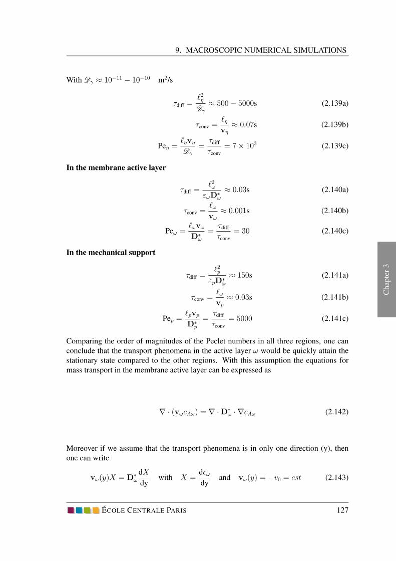
9. MACROSCOPIC NUMERICAL SIMULATIONS
Chap
ter
3
With Dγ ≈ 10−11 − 10−10 m2/s
τdiff =ℓ2ηDγ
≈ 500− 5000s (2.139a)
τconv =ℓηvη
≈ 0.07s (2.139b)
Peη =ℓηvη
Dγ
=τdiff
τconv
= 7× 10³ (2.139c)
In the membrane active layer
τdiff =ℓ2ω
εωD∗ω
≈ 0.03s (2.140a)
τconv =ℓωvω
≈ 0.001s (2.140b)
Peω =ℓωvω
D∗ω
=τdiff
τconv
= 30 (2.140c)
In the mechanical support
τdiff =ℓ2p
εpD∗p
≈ 150s (2.141a)
τconv =ℓωvp
≈ 0.03s (2.141b)
Pep =ℓpvp
D∗p
=τdiff
τconv
= 5000 (2.141c)
Comparing the order of magnitudes of the Peclet numbers in all three regions, one can
conclude that the transport phenomena in the active layer ω would be quickly attain the
stationary state compared to the other regions. With this assumption the equations for
mass transport in the membrane active layer can be expressed as
∇ · (vωcAω) = ∇ ·D∗ω · ∇cAω (2.142)
Moreover if we assume that the transport phenomena is in only one direction (y), then
one can write
vω(y)X = D∗ω
dX
dywith X =
dcωdy
and vω(y) = −v0 = cst (2.143)
ECOLE CENTRALE PARIS 127

Chap
ter3
CHAPTER 2. UPSCALED MODELING OF MICROLTRATION MEMBRANE
FOULING BY PROTEIN SOLUTIONS : THEORETICAL STUDY
Figure 2.10: Concentration difference in the fluid and porous medium region for different
values of Pe numbers.
Eq. (2.143) can be analytically solved
Xω(y) = Xω(0)exp
(−v0D∗
ω
y
)
(2.144)
cω(y) = cω(0)−Xω(0)D∗
ω
v0
[
exp
(−v0D∗
ω
y
)
− 1
]
(2.145)
and then
cω(y)− cω(0)
cω(ℓω)− cω(0)=
exp
(
−v0y
D∗ω
)
− 1
exp
(
−v0ℓωD∗
ω
)
− 1
=
1− exp
(
-Peωy
ℓω
)
1− exp (-Peω)(2.146)
128 ECOLE CENTRALE PARIS

10. CONCLUSIONS AND DISCUSSION
Chap
ter
3
Assuming the stationary state in the ω region, the flux passing through any cross
section of the ω-region in the increasing y direction will be conserved which gives rise to
φω = y · εω (D∗ω∇cω + vycω) (0) = y · εω (−D∗
ω∇cω + vycω) (ℓω) (2.147)
φω is given by
φω = −εω
(
D∗ω
dcωdy
(0) + vycω(0)
)
= −εω (D∗ωXω(0)− v0cω(0))
=[cω(0)− cω(ℓω)] v01− exp (−Peω)
− v0cω(0) (2.148)
To summarize at the new dividing surface η − p, we will have the continuity of the total
flux and a jump condition for the concentration field.
− n · (−Dγ∇cη + v0cη) = −εpn ·(−D∗
p∇cp + v0cp)
cp − cη =
[ℓωD∗
ω
φ+ Peωcp
] [1− exp (−Peω)
(Peω)
]
=ℓωD∗
ω
[1− exp (−Peω)
(Peω)
]
(2.149)
And φ is the convective-diffusive flux passing through the η − p interface in the p − ηdirection
φ = −εpnpη ·(D∗
p∇cp + vpcp)= npη · (−Dγ∇cη + vηcη) (2.150)
This new jump condition imposes the continuity of the fluxes and jump in the concentra-
tion fields at the new η − p dividing surface which can only be assumed in a stationary
state situation in the membrane active layer whilst the governing equations in the fluid
phase and membrane porous support may remain time dependent. The main advantage
of this new jump condition is that the concentration difference between fluid and support
porous medium is directly related to the mass transfer phenomena in the active layer. The
jump in the concentration is due to mass transfer in the membrane active layer. The results
of this new jump condition are presented in Fig. 2.10. The analytical expression of the
concentration difference in the fluid phase and porous medium is given in Eq. (2.149).
The results proved that for low Peclet numbers, the concentration jump is only due to
the diffusion in the active layer (ℓωD∗
ω
). However for considerable values of Peclet number
(≫ 103), the right hand term in equation (2.149) becomes null and thus the concentration
filed remains continuous.
10 CONCLUSIONS AND DISCUSSION
During the filtration process of protein solutions through the membranes, adsorption to
the membrane interface is one of the fouling mechanisms leading to membrane pore
ECOLE CENTRALE PARIS 129
Chap
ter3
CHAPTER 2. UPSCALED MODELING OF MICROLTRATION MEMBRANE
FOULING BY PROTEIN SOLUTIONS : THEORETICAL STUDY
size reduction and consequent permeate flux decline. Different studies have shown that
the protein adsorption to the membrane inner pores affects the membrane performance
irreversibly[7],[132], [149],[162],[207].
The objective of this chapter was to develop an upscaled model for description of
protein adsorption during a filtration process. Experiments confirmed that membrane is
composed of three layers. It should be pointed out that in reality, proteins may trans-
port and adsorb in all membrane layers, However, we have assumed that the variations
of permeabilities in membrane layers due to protein adsorption are negligible except for
the membrane active layer.Thus, in the first study, we only developed a model of protein
adsorption in a very thin active layer of the membrane. An original averaged descrip-
tion of the membrane structure was described. Instead of determination the additional
resistances in terms of observed mechanisms, we derived the evolution of the membrane
structure with time. Convection and diffusion were taken into account as local trans-
port phenomena. Adsorption is the result of mass transport between membrane and the
fluid phase and it represented the interfacial phenomenon. The volume averaging method
is used for deriving the upscaled equations from their local counterparts.The simplifi-
cations of different terms (with contribution on pore-scale and membrane-scale transport
mechanisms) were based on estimation of order of magnitudes or length-scale constraints
(e.g. interfacial velocity due to adsorption was neglected compared to average velocity
field [29]). A classical closure problem for the momentum transport has been identi-
fied whereas the closure problem for the mass conservation equation included two source
terms (due to diffusion and adsorption).The upscaled closed set of equations in the fluid
phase consist of the averaged continuity equation, non-stationary Stokes equation for mo-
mentum transport, the direct expression of its porosity in function of adsorption rate and
averaged mass conservation equation for proteins. The accumulation term in the upscaled
mass conservation equation is modified and includes the adsorption phenomenon at the
interface. Compared to the classical models [255], the upscaled equations of mass and
momentum transport both represented explicit expressions of porous structural evolution
with time.
Experiments are directly coupled with the model development at two levels: the pore
scale experiments are done to characterize the membrane structure and proteins adsorp-
tion isotherms. The local diffusivity of the proteins is also needed as initial data and is
taken from literature. The microfiltration experiments confirmed that protein adsorption is
a complicated phenomenon in which different parameters (solution chemistry, membrane
properties, operational conditions) play important roles. The effect of these parameters
are not involved in the proposed model and can be subject of future study. It is with to
mention that the electrostatic interactions between particles and the membrane surface
could be taken into account by adding some source terms in the local equations of the
mass transport. In the work of [258] the Smoluchowski has been used to understand the
effect of these interactions on the mass transport phenomena. However the experimental
characterization of these interactions remains challenging both at local and macroscopic
scales.
130 ECOLE CENTRALE PARIS
10. CONCLUSIONS AND DISCUSSION
Chap
ter
3
Since the closure problems for both mass and momentum transport equations were clas-
sical, we have used the expression of the effective diffusivity (Maxwell) and permeability
(Kozeny-carman) to determine these effective properties in the membrane active layer
and support porous structure.
Consequently the macroscopic numerical simulations were run to validate the system
performance qualitatively. The membrane active layer was replaced with a (virtual) di-
viding surface between bulk fluid and the support porous medium. Here we recall that the
jump conditions were assumed only to overcome the numerical difficulties related to the
small characteristic length of the membrane active layer. Two cases have been studied:
In the first study, a jump condition for the mass flux was imposed which was due to the
adsorption in the active layer of the membrane, however the continuity of the intrinsic
concentrations in the bulk fluid and the membrane porous medium was assumed. In the
second study, a jump condition for the concentration fields and a condition of the conti-
nuity of the mass flux was supposed. This second condition could be applied only if the
transport phenomenon in the active layer would attain the stationary state. Another study
which contains a jump condition both for the concentration fields and mass flux would be
subject of the future study.
ECOLE CENTRALE PARIS 131

UPSCALED MODELING OF MASS AND
MOMENTUM TRANSPORT IN BIOFILMS 3
ECOLE CENTRALE PARIS 133

Chap
ter4
CHAPTER 3. UPSCALED MODELING OF MASS AND MOMENTUM
TRANSPORT IN BIOFILMS
List of symbols
−β Related to the fluid phase
−ω Related to the EPS region
−σ Related to the cell region
−η Related to the water channel region
Aηω interfacial area contained within the biofilm between η− ω regions, m2
Aωσ interfacial area contained within the biofilm between ω− σ regions, m2
bηωα second-order tensor used to represent Tα at η − ω interface
Bηωα second-order tensor used to represent vα at η − ω interface
ciη concentration of species i is the η region, molm−3
ciω concentration of species i is the ω region, molm−3
ciσ concentration of species i is the σ region, molm−3
〈ciη〉 superficial average concentration of species i in the η region, molm−3
〈ciη〉η intrinsic average concentration of species i in the η region, molm−3
〈ciω〉 superficial average concentration of species i in the ω region, molm−3
〈ciω〉ω intrinsic average concentration of species i in the ω region, molm−3
〈ciσ〉 superficial average concentration of species i in the σ region, molm−3
〈ciσ〉σ intrinsic average concentration of species i in the σ region, molm−3
{ci} equilibrium weighed average concentration for species i, molm−3
ciη biofilm-scale spatial deviation for species i in the η-region
ciω biofilm-scale spatial deviation for species i in the ω-region
ciσ biofilm-scale spatial deviation for species i in the σ-region
ciη spatial deviation concentration for species i in the η region,molm−3
ciω spatial deviation concentration for species i in the ω region,molm−3
ciσ spatial deviation concentration for species i in the σ region,molm−3
cηωω vector used to represent pη at the ηω interface, m−1
cωσω vector used to represent pη at the σω interface, m−1
diη vector field used to represent ciηdiω vector field used to represent ciωdiσ vector field used to represent ciσDiη mixture diffusivity for species i in η region, m2s−1
Diω mixture diffusivity for species i in ω region, m2s−1
Diσ mixture diffusivity for species i in σ region, m2s−1
134 ECOLE CENTRALE PARIS

0.
Chap
ter
4
Di,eff effective diffusivity for species i in the biofilm, m2s−1
Di,dis effective dispersion for species i in the biofilm, m2s−1
E0 surface concentration of transporter proteins for cell productions,
molm−2
KA half saturation constant for Monod kinetic form, molm−3
kωσi cell membrane permeability for species i (at ω − σ interface)
kωηi mass transfer coefficient for species i (at ω − σ interface)
Keq,B phase equilibrium coefficient for species B
Keq,C phase equilibrium coefficient for species C
Keq,D phase equilibrium coefficient for species D
Kω permeability tensor of ω-region (EPS fibers) (m2)
Kωσ permeability tensor of ω − σ-region (biofilm matrix) (m2)
K permeability tensor of the biofilm
ℓηω local-scale characteristic length associated with η − ω region, m
ℓωσ local-scale characteristic length associated with ω − σ region, m
ℓη Characteristic length for the η-region, m
ℓω Characteristic length for the η-region, m
ℓσ Characteristic length for the σ-region, m
ℓbf Characteristic length for the biofilm, m
L Characteristic length for the averaged volume, m
Mi molar weight of species i, kgmol−1
nηω -nωη, unit normal vector directed from the η-region to ω-region
nωσ -nσω, unit normal vector directed from the ω-region to σ-region
nωη ·wωη displacement velocity at ω − η interface
nωσ ·wωσ displacement velocity at ω − σ interface
pβ local pressure of β phase (fluid), Pa
pη local pressure of η region, Pa
pω local pressure of ω region, Pa
〈pη〉η intrinsic average pressure in the η region, Pa
〈pω〉ω intrinsic average pressure in the ω region, Pa
{p} equilibrium pressure in the biofilm, Pa
pη spatial deviation of pressure in the η region, Pa
pω spatial deviation of pressure in the ω region, Pa
r0 radius of the averaging volume, m
Ri rate of production of species i in the σ-region, molm−2s−1
Tβ viscous stress tensor of β phase (fluid), Pa
ECOLE CENTRALE PARIS 135

Chap
ter4
CHAPTER 3. UPSCALED MODELING OF MASS AND MOMENTUM
TRANSPORT IN BIOFILMS
Tη viscous stress tensor of η region, Pa
Tω viscous stress tensor of ω region, Pa
Tσ viscous stress tensor of η region, Pa
〈Tη〉η intrinsic average viscous tensor of η region, Pa
〈Tω〉ω intrinsic average viscous tensor of ω region (fluid), Pa
Tη intrinsic average viscous tensor of η region, Pa
Tω intrinsic average viscous tensor of ω region, Pa
viη velocity of species i in the η-region, ms−1
viω velocity of species i in the ω-region, ms−1
viσ velocity of species i in the σ-region, ms−1
vη velocity of the η-region, ms−1
vω velocity of the ω-region, ms−1
vσ velocity of the σ-region, ms−1
〈vη〉 superficial average velocity of η region, ms−1
〈vη〉η intrinsic average velocity of η region, ms−1
〈vω〉 superficial average velocity of ω region, ms−1
〈vω〉ω intrinsic average velocity of ω region, ms−1
{v} equilibrium velocity in the biofilm,ms−1
vη spatial deviation of the velocity in the η region, ms−1
vω spatial deviation of the velocity in the ω region, ms−1
V averaging volume m−3
Vη volume of the η-region in the averaged volume m−3
Vω volume of the ω-region in the averaged volume m−3
Vσ volume of the σ-region in the averaged volume m−3
136 ECOLE CENTRALE PARIS

0.
Chap
ter
4
Greek letters
α1 equilibrium coefficient defined in reaction equation
α2 reaction rate parameter in cells, mol s m−3
α3 reaction rate parameter in cells, s
α4 reaction rate parameter in cells, s
α5 reaction rate parameter in cells, m3s mol−1
εη volume fraction of the η-region
εω volume fraction of the ω-region
εσ volume fraction of the σ-region
µA maximum specific substrate utilization parameter, molm3s−1
µβ Dynamic viscosity of the fluid phase, Pa.s
ρiη mass density of species i in the η-region, kg m−3
ρiω mass density of species i in the ω-region, kg m−3
ρiσ mass density of species i in the σ-region, kg m−3
ρη total mass density in the η-region, kg m−3
ρω total mass density in the ω-region, kg m−3
ρσ total mass density in the σ-region, kg m−3
〈ρη〉η intrinsic average mass density in the η-region, kg m−3
〈ρω〉ω intrinsic average mass density in the ω-region, kg m−3
〈ρσ〉σ intrinsic average mass density in the σ-region, kg m−3
{ρ} equilibrium mass density in the biofilm, kg m−3
ρη spatial deviation mass density in the η-region
ρω spatial deviation mass density in the ω-region
ρσ spatial deviation mass density in the σ-region
ECOLE CENTRALE PARIS 137

Chap
ter4
CHAPTER 3. UPSCALED MODELING OF MASS AND MOMENTUM
TRANSPORT IN BIOFILMS
A biofilm is an assemblage of surface-associated microbial cells embedded in a slimy
matrix of extracellular polymeric compounds. Biofilms are ubiquitous in natural and in-
dustrial systems. Among the problems associated with biofilms, energy losses, equipment
damage, product contamination and medical infections are reported. In the particular
case of membrane filtration systems, biofilm development induces a decline of process
performance. Consequently cleaning procedures and replacement of the membranes are
required. Biofilm development is a very complicated process governed by several cou-
pled physical, chemical and biological phenomena. Mathematical modeling of biofilms
is then crucial to get a better understanding of involved phenomena. It is an essential tool
to make predictions that might help enhancing or reducing biofilm formation.
Several modeling approaches describing biofilm development have been proposed since
the early 1980s. The description of the highly heterogeneity of biofilms in space and
time is challenging. Recently, models and techniques developed for porous media have
been used to study biofilms. In these models, mechanisms at microscopic scale are first
identified and described. Afterwards, by using an upscaling method, the description of
macroscopic phenomena is obtained.
The goal of this study is to propose an upscaled biofilm model that takes into account
transport (diffusion and convection) and reaction mechanisms at biofilm scale. At micro-
scopic scale, the biofilm is represented by a set of three regions (cells, exopolysaccharides
gel and water channels). The gelatinous EPS region is composed itself by two phases, a
fluid and a solid (EPS fibers). First, conservation equations for mass and momentum
transport are derived for each region, in unsteady state. Thereafter, a first upscaling with
the volume averaging method is applied to reach a scale (intermediate scale) where the
EPS matrix can be described as a continuum. Another upscaling is then performed to
reach biofilm scale (macroscopic scale). Local mass and momentum equilibrium cases
are presented in this work. Although, non-equilibrium conditions are more realistic, they
are rarely assumed in models described in the literature. Our model is able to predict the
evolution with time of the biofilm structural properties (porosity, diffusivity, permeabil-
ity) and the profiles of species concentration and velocities. Numerical simulations are
performed to determine the total permeability tensor of the biofilm which includes both
permeabilities of the EPS fibers and biofilm matrix.
138 ECOLE CENTRALE PARIS

1. INTRODUCTION
Chap
ter
4
1 INTRODUCTION
A biofilm is an assemblage of surface-associated microbial cells that are enclosed in a
matrix of hydrated Extracellular Polymeric Substances (EPS) mainly composed of ex-
opolysacharides, proteins and nucleic acids [38]. Non cellular materials such as mineral
crystals, corrosion particles, clay or blood components depending on the environment in
which the biofilm was developed, may also be found in biofilm matrix.
Biofilms may form on a wide variety of surfaces including living tissues, medical or
dental devices, industrial or potable water system piping, in dairy industry and in natural
aquatic systems. Biofilm formation (biofouling) causes technical and economic losses
in many industries and in medical environments. Corrosion [145], energy losses and
blockages in condenser tubes, membrane systems, water [146] and wastewater circuits,
heating systems [128], heat exchangers, and even on ship hulls have been associated
with biofilms. General processes leading to biofilm formation are the following: (1) pre-
conditioning of the material surface by macromolecules from the aqueous medium, (2)
Transport of cells in suspension (planktonic cells) from the bulk liquid to the surface,
followed by reversible (3) and irreversible (4) adsorption of cells, (5) biofilm growth and
polymers excretion on the surface, (6) biofilm detachment, erosion and sloughing [227].
The attachment of microorganisms to surfaces and subsequent biofilm development are
very complex processes, strongly affected by several variables associated to cell prop-
erties, the substratum and the surrounding environmental conditions of the bulk liquid
[70],[71].
Biofilm architecture is heterogeneous, both in space and time, constantly changing due
to internal and external processes. It contains microcolonies encased in the EPS ma-
trix separated from other micro-colonies by interstitial voids (water channels). Liquid
flow occurs in these water channels allowing diffusion of nutrients, metabolites and even
antimicrobial agents [70], [50],[23]. Biofilm structure is largely influenced by environ-
mental conditions including the nutrient diffusion, convection and bulk shear stress. Ad-
ditionally, sessile microorganisms (biofilm associated organisms) differ largely from their
planktonic counterparts (freely suspended) concerning genes transcription.
The understanding and modeling of mass transport and reaction in biofilms has devel-
oped substantially in the past decades. Nowadays, mathematical modeling is an essential
tool to understand the phenomena (physical, chemical and biological) involved in biofilm
development and activity. It also helps providing clues to struggle against biofouling in
engineering systems and to predict process performances in different industrial applica-
tions.
One critical point that should be taken into account when developing a biofilm model is
its heterogeneity 1) Structural: biofilm thickness, roughness, porosity and relative perme-
ability; 2) Chemical: gradient of chemical species, pH variations which induce and create
a high diversity of reactions (aerobic and anaerobic); 3) Biological: diversity of microbial
species and physiological states (growing and dead cells, at different growth rates)and 4)
ECOLE CENTRALE PARIS 139

Chap
ter4
CHAPTER 3. UPSCALED MODELING OF MASS AND MOMENTUM
TRANSPORT IN BIOFILMS
Physical: biofilm density and viscosity, EPS properties, species diffusivity in the matrix
[60].
Moreover, very different length scales are found in a biofilm. They vary from a few
nanometers (size of extracellular polymeric fibers), to several micrometers or centimeters
(biofilm thickness), with the size of bacterial cells (1 − 2 µm) as an intermediate length
scale.
The first attempts of biofilm modeling consisted in the development of continuum models
primarily in one space dimension [106]. Here, biofilms are described as homogenous and
continuous structures. In these models, the evolution of biofilm thickness and the spatial
distribution of microbial species and nutrients in the biofilm are predicted with time.
Additionally, diffusion is usually the only transport phenomenon taken into account. Due
to their simplicity, one-dimensional biofilm models have difficulties characterizing the
multidimensional biofilm structure [245].
The Cellular Automaton (CA) model has been widely applied to model biofilm hetero-
geneous structures. When CA model is used, the physical space is divided in an array
of small compartments, which are allowed to fill up with biomass to a predetermined
maximum. Once a compartment is full or overflowing, a simple rule-based system is
employed in order to locate the compartment in which the extra biomass will be placed.
For example, the generation of a new cell in one compartment requires that the CA al-
gorithm decides where to locate the new cell, based on the occupancy of neighboring
compartments. The decisions are made based on a set of rules that act locally, but ap-
ply globally [54]. Although the main principles are the same, the rules governing the
biomass spreading differ from a model to another. The randomness in the step of biomass
distribution is pointed out as a drawback of this approach. Literature contains CA mod-
els that incorporate the following biological mechanisms: cell division, cell movement,
cell to cell communication and diffusion of nutrients[196], [199], [245]. However the
influence of surrounding fluid is not included in CA modeling approach. However, it was
also found that the hydrodynamics of the bulk fluid plays an important role in shaping
the structure of biofilms [71] through both the nutrients convection and the detachment
of biomass by shear stress. Therefore, more recently, several biofilm models coupling
biofilm development to bulk fluid were developed [199],[200],[202].
More recently, an increasing interest of the research community in considering the multi-
scale characteristics of a biofilm (from the nanometer (EPS, protein in the matrix) to the
millimeter/centimeter (biofilm thickness)) in model development is reported. The idea
that biofilm models should be upscaled directly from microscopic scale has been first
proposed by Wanner and Gujer [248],[251]. The main advantages of the upscaled tech-
niques, in general, and the volume averaging, in particular, are the following: 1) the
resulting model relates the microscopic parameters to the observable macroscopic ones.
For instance, the effective diffusivity at macroscopic scale takes into account local diffu-
sivities, the microstructure and dispersion caused by the local velocity field; 2) indicates
under what conditions the conservation equations (mass, momentum) are valid.
These works include upscaling reactive solute transport within the matrix, cellular growth
140 ECOLE CENTRALE PARIS

2. PRESENTATION OF THE MODEL
Chap
ter
4
and diffusion of nutrients. In addition, the effective properties provide some additional
information from both local (cell) scale and biofilm structure (porosity. . . ) [260], [262],
[263].
In general, most of the work with the volume averaging method focused on local mass
equilibrium conditions in a representative elementary volume and on the continuity or
not (jump conditions) of quantities at the interface between phases in a porous region or
between porous regions. Under these circumstances, all intrinsic concentrations can be
assumed to be equal in a representative elementary volume and one mass balance equation
is sufficient to describe mass transport. However, it should be noted that non-equilibrium
conditions with moving interfaces are closer to reality.
2 PRESENTATION OF THE MODEL
During filtration of water containing bacteria through a porous membrane, the microor-
ganisms that are present can attach to the membrane surface and form a biofilm that will
progressively decrease the performance of the process by increasing the resistance to the
flow (or decreasing global permeability). This phenomenon causes a fouling of the mem-
brane in surface. Furthermore, the biofilm produces chemical species that can enter the
membrane and eventually lead to its fouling in volume.
A model for membrane fouling in volume caused by adsorption has already been de-
veloped in another article and the objective of this work is to model the influence of the
biofilm on fouling. It aims at predicting first the evolution with time of the species concen-
tration profiles and particularly at the biofilm-membrane interface, in order to give input
data for the adsorption model, and secondly the evolution with time of the biofilm struc-
tural parameters (porosities, dimensions), in order to quantify its impact on the global
permeability.
The smallest scale considered in this study is the continuum mechanics one. At this
scale, the resolution of transport phenomena equations inside the biofilm would be very
complex and very demanding numerically. Therefore, the model developed here provides
convection-diffusion-reaction balance equations at biofilm scale by upscaling with the
volume averaging method, starting from equations at continuum mechanics scale. When
a description at large scale is needed, this method has the advantage to provide a link with
phenomena at small scale, which avoids using empirical laws.
As the objective of this first model is to obtain qualitative results, many simplifying
hypotheses are made. Neither the initial attachment of the cells to the membrane
surface or the biofilm detachment due to shear stress will be taken into account (see
[199],[201],[213] for additional information). The model only deals with an already
existing layer of biofilm contaning bacteria in the same biological state. Here, the
biofilm is described geometrically by a parallelepiped completely covering the top
rectangular surface of the membrane and only its thickness can evolve with time. No
spatial distribution of the structural biofilm parameters is considered in this first version
ECOLE CENTRALE PARIS 141

Chap
ter4
CHAPTER 3. UPSCALED MODELING OF MASS AND MOMENTUM
TRANSPORT IN BIOFILMS
of the model. In future work, the model will be able to treat a biofilm made of several
layers and biofilm heterogeneity with space and time will then be taken into account.
The presence of the supporting membrane will only be accounted for through boundary
conditions at biofilm scale.
From a structural point of view, the biofilm is represented as a set of three regions: a
cellular region (σ), a gelatinous region (ω) and a fluid region (η). The σ-region, composed
of all the microorganisms in the system, is modeled as a fluid. The cell wall, and in
particular its barrier effect for species, is taken into account in the boundary conditions
at the ω − σ interface, using a simple carrier model [137], [138]. For their growth,
and following [260, 261], bacteria use a substrate (species A) and an electron acceptor
(species B) to form EPS (species C), terminal products (species D) and intercellular
products (species E) which increase the cell mass. While species E always remains in
the cell, the other species can enter or leave bacteria. Species D is assumed to be water
only. The reaction model is represented in Fig.3.1.
Figure 3.1: Reactants and products in a bacterial cell
The ω-region is a two-phase porous medium containing a solid phase made of EPS fibers
and a fluid phase made of a mixture of species A, B, C diluted in water (D). The η-
region represents biofilm water channels and contains the same kind of mixture. Because
the biofilm is already formed, it is plausible to assume that the cell region σ is completely
surrounded by the EPS region ω and that there is no contact between σ and η-regions. All
the regions with their characteristic length scales are presented in Fig. 3.2.
First, balance equations will be written at the smallest scale considered here, e.g. the
continuum mechanics scale (microscopic scale) in unsteady state, in order to obtain at
the end time evolution of macroscopic quantities. Using the Representative Elementary
Volume (REV) described in Fig. 3.3, the volume averaging method will then be used in
the three regions to reach a scale where the ω-region can be described as a one-phase
continuum (intermediate scale). Another upscaling will then be applied to get to the
biofilm scale (macroscopic scale), in the cases of local mass/momentum equilibrium and
non-equilibrium. Many existing models make the assumption of local equilibrium, but
142 ECOLE CENTRALE PARIS

2. PRESENTATION OF THE MODEL
Chap
ter
4
Figure 3.2: Hiearchical biofilm structure with constituting regions of interest
in fact, it relies on precise time and length scale constraints that are not always verified.
Transport properties at macroscopic scale, such as permeability and effective diffusivity,
will be determined by solving associate problems, called closure problems, in domains at
small scale that are representative of the biofilm structure. These properties are functions
of small scale parameters such as structure and biophysical properties. The evolution
with time of macroscopic quantities (concentration fields, velocity fields, porosities) will
finally be determined.
In future work, a link between the evolution with time of the biofilm thickness and these
macroscopic quantities will be determined, modeling the biofilm growth. Experimental
data will also be performed to characterize properties at microscopic scale (diffusivities,
equilibrium constants. . . ) and at macroscopic scale (initial porosities) and to validate the
numerical results of the macroscopic model.
ECOLE CENTRALE PARIS 143

Chap
ter4
CHAPTER 3. UPSCALED MODELING OF MASS AND MOMENTUM
TRANSPORT IN BIOFILMS
Figure 3.3: Representative Elementary Volume of the biofilm matrix with characteristic
length scale of each region
3 MODEL AT MICROSCOPIC SCALE
3.1 ω-REGION (EPS GEL)
As seen in Fig. 3.2, the ω-region is composed of two phases, namely a fluid phase β and
a solid phase κ (EPS fibers). It is assumed that the microstructure of this region does not
evolve anymore. Microscopic conservation equations in the ω-region are
∂ρβ∂t
+∇ · (ρβvβ) = 0 in the β-phase (3.1a)
∂ (ρβvβ)
∂t= ρβg +∇ · Tβ in the β-phase (3.1b)
∂ciβ∂t
+∇ · (ciβviβ) = 0 i = A→ C in the β-phase (3.1c)
cEβ = 0 in the β-phase (3.1d)
144 ECOLE CENTRALE PARIS
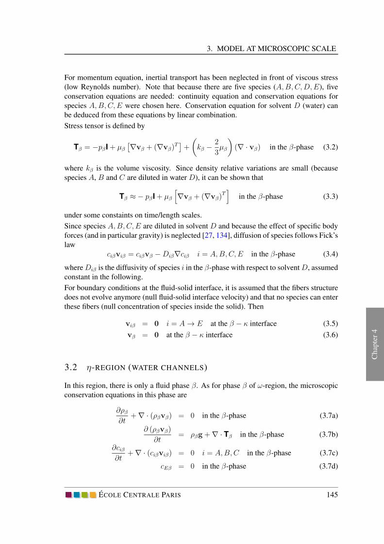
3. MODEL AT MICROSCOPIC SCALE
Chap
ter
4
For momentum equation, inertial transport has been neglected in front of viscous stress
(low Reynolds number). Note that because there are five species (A,B,C,D,E), five
conservation equations are needed: continuity equation and conservation equations for
species A,B,C,E were chosen here. Conservation equation for solvent D (water) can
be deduced from these equations by linear combination.
Stress tensor is defined by
Tβ = −pβI + µβ
[∇vβ + (∇vβ)
T]+
(
kβ −2
3µβ
)
(∇ · vβ) in the β-phase (3.2)
where kβ is the volume viscosity. Since density relative variations are small (because
species A, B and C are diluted in water D), it can be shown that
Tβ ≈− pβI + µβ
[
∇vβ + (∇vβ)T]
in the β-phase (3.3)
under some constaints on time/length scales.
Since species A,B,C,E are diluted in solvent D and because the effect of specific body
forces (and in particular gravity) is neglected [27, 134], diffusion of species follows Fick’s
law
ciβviβ = ciβvβ −Diβ∇ciβ i = A,B,C,E in the β-phase (3.4)
whereDiβ is the diffusivity of species i in the β-phase with respect to solventD, assumed
constant in the following.
For boundary conditions at the fluid-solid interface, it is assumed that the fibers structure
does not evolve anymore (null fluid-solid interface velocity) and that no species can enter
these fibers (null concentration of species inside the solid). Then
viβ = 0 i = A→ E at the β − κ interface (3.5)
vβ = 0 at the β − κ interface (3.6)
3.2 η-REGION (WATER CHANNELS)
In this region, there is only a fluid phase β. As for phase β of ω-region, the microscopic
conservation equations in this phase are
∂ρβ∂t
+∇ · (ρβvβ) = 0 in the β-phase (3.7a)
∂ (ρβvβ)
∂t= ρβg +∇ · Tβ in the β-phase (3.7b)
∂ciβ∂t
+∇ · (ciβviβ) = 0 i = A,B,C in the β-phase (3.7c)
cEβ = 0 in the β-phase (3.7d)
ECOLE CENTRALE PARIS 145

Chap
ter4
CHAPTER 3. UPSCALED MODELING OF MASS AND MOMENTUM
TRANSPORT IN BIOFILMS
with
Tβ ≈− pβI + µβ
[∇vβ + (∇vβ)
T]
in the β-phase (3.8)
and
ciβviβ = ciβvβ −Diβ∇ciβ i = A,B,C,E in the β-phase (3.9)
3.3 σ-REGION (CELLS)
In this region, there is only a fluid phase γ. A biochemical process occurs there, repre-
sented by the reaction
A+ η1B → η2C + η3D + η4E (3.10)
The molar reaction rate for species i, Ri, is assumed to have a Michaelis-Menten form
[261], with a limiting substrate (A) and an electron acceptor (B) in excess. The micro-
scopic conservation equations in this phase are then
∂ργ∂t
+∇ · (ργvγ) = 0 in the γ-phase (3.11a)
∂ (ργvγ)
∂t= ργg +∇ · Tγ in the γ-phase (3.11b)
∂ciγ∂t
+∇ · (ciγviγ) = Ri(cAγ) i = A,B,C,E in the γ-phase (3.11c)
with
Tγ ≈ −pγI + µγ
[∇vγ + (∇vγ)
T]
in the γ-phase (3.12)
ciγviγ = ciγvγ −Diγ∇ciγ i = A,B,C,E in the γ-phase (3.13)
and molar reaction rates depending only on cAγ
RA(cAγ) = −µAcAγ
KA + cAγ
in the γ-phase (substrate) (3.14a)
RB(cAγ) = −η1µAcAγ
KA + cAγ
in the γ-phase (electron acceptor) (3.14b)
RC(cAγ) = +η2µAcAγ
KA + cAγ
in the γ-phase (EPS) (3.14c)
RD(cAγ) = +η3µAcAγ
KA + cAγ
in the γ-phase (water) (3.14d)
RE(cAγ) = +η4µAcAγ
KA + cAγ
in the γ-phase (intercellular products)(3.14e)
The equalityMA+η1MB = η2MC+η3MD+η4ME , which leads to∑
i=A→E MiRi(cAγ) =0, was also used to obtain (3.11a).
146 ECOLE CENTRALE PARIS

4. UPSCALED MODEL AT INTERMEDIATE SCALE
Chap
ter
4
4 UPSCALED MODEL AT INTERMEDIATE SCALE
In the next equations, according to [255], the definition of superficial average of any
function associated with an α-phase or α-region (α = β, γ, ω, η, σ) is used
〈ψα〉 =1
V
∫
Vα(t)
ψαdV (3.15a)
as well as the definition of the intrinsic average
〈ψα〉α =
1
Vα(t)
∫
Vα(t)
ψαdV (3.15b)
The region where the average is taken is designated with an index: for example 〈ψβ〉ω is
the superficial average of ψβ (defined in the β-phase) in the ω-region.
4.1 ω-REGION (EPS GEL)
The volume-averaged form of the conservation equations can be written as
∂〈ρβ〉βω
∂t+∇ · (〈ρβ〉
βω〈vβ〉
βω) = 0 in the ω-region (3.16a)
∂(〈ρβ〉
βω〈vβ〉
βω
)
∂t= 〈ρβ〉
βωg +∇ · 〈Tβ〉
βω − µβK
−1 · εβ,ω〈vβ〉βω in the ω-region
(3.16b)
∂〈ciβ〉βω
∂t+∇ · (〈ciβ〉
βω〈vβ〉
βω) = Diβ∇
2〈ciβ〉βω i = A→ C in the ω-region (3.16c)
〈cEβ〉βω = 0 in the ω-region (3.16d)
with
〈Tβ〉βω = −〈pβ〉
βωI + µβ
[
∇〈vβ〉βω +
(∇〈vβ〉
βω
)T]
in the ω-region (3.17)
and K denotes the permeability tensor, which is uniform and constant with time because
the fibrous structure does not evolve. In deriving the above expressions, the dispersive
transport was assumed negligible compared to the convective one and the fact that the
porosity εβ,ω is uniform and constant with time was used.
ECOLE CENTRALE PARIS 147

Chap
ter4
CHAPTER 3. UPSCALED MODELING OF MASS AND MOMENTUM
TRANSPORT IN BIOFILMS
To simplify notations, the following changes are made
〈ρβ〉βω → ρω (3.18a)
〈vβ〉βω → vω (3.18b)
〈pβ〉βω → pω (3.18c)
K−1εβ,ω → K
−1ω (3.18d)
〈ciβ〉βω → ciω (3.18e)
〈viβ〉βω → viω (3.18f)
so that Eqs. (3.16) take the form
∂ρω∂t
+∇ · (ρωvω) = 0 in the ω-region (3.19a)
∂ (ρωvω)
∂t= ρωg +∇ · Tω − µβK
−1ω · vω in the ω-region (3.19b)
∂ciω∂t
+∇ · (ciωvω) = Diβ∇2ciω i = A→ C in the ω-region (3.19c)
cEω = 0 in the ω-region (3.19d)
with
Tω = −pωI + µβ
[
∇vω + (∇vω)T]
in the ω-region (3.20)
4.2 η-REGION (WATER CHANNELS)
Applying an averaging operator of the same size as the one used for the ω-region and
because there is no fluid-solid interface, and with the same kind of assumptions as for the
ω-region
∂〈ρβ〉βη
∂t+∇ · (〈ρβ〉
βη 〈vβ〉
βη ) = 0 in the η-region (3.21a)
∂(〈ρβ〉
βη 〈vβ〉
βη
)
∂t= 〈ρβ〉
βηg +∇ · 〈Tβ〉
βη in the η-region (3.21b)
∂〈ciβ〉βη
∂t+∇ · (〈ciβ〉
βη 〈vβ〉
βη ) = Diβ∇
2〈ciβ〉βη i = A→ C in the η-region (3.21c)
〈cEβ〉βη = 0 in the η-region (3.21d)
with
〈Tβ〉βη = −〈pβ〉
βη I + µβ
[
∇〈vβ〉βη +
(∇〈vβ〉
βη
)T]
in the η-region (3.22)
148 ECOLE CENTRALE PARIS

4. UPSCALED MODEL AT INTERMEDIATE SCALE
Chap
ter
4
To simplify notations, the following changes are made
〈ρβ〉βη → ρη (3.23a)
〈vβ〉βη → vη (3.23b)
〈pβ〉βη → pη (3.23c)
〈ciβ〉βη → ciη (3.23d)
〈viβ〉βη → viη (3.23e)
so that conservation equations for this region can be written as
∂ρη∂t
+∇ · (ρηvη) = 0 in the η-region (3.24a)
∂ (ρηvη)
∂t= ρηg +∇ · Tη in the η-region (3.24b)
∂ciη∂t
+∇ · (ciηvη) = Diβ∇2ciη i = A→ C in the η-region (3.24c)
cEη = 0 in the η-region (3.24d)
with
Tη = −pηI + µβ
[
∇vη + (∇vη)T]
in the η-region (3.25)
4.3 σ-REGION (CELLS)
Following the same method as for η-region, conservation equations at this scale are
∂〈ργ〉γσ
∂t+∇ · (〈ργ〉
γσ〈vγ〉
γσ) = 0 in the σ-region (3.26a)
∂ (〈ργ〉γσ〈vγ〉
γσ)
∂t= 〈ργ〉
γσg +∇ · 〈Tγ〉
γσ in the σ-region (3.26b)
∂〈ciγ〉γσ
∂t+∇ · (〈ciγ〉
γσ〈vγ〉
γσ) = Diγ∇
2〈ciγ〉γσ +Ri(〈cAγ〉
γσ) i = A,B,C,E in the σ-region
(3.26c)
with
〈Tγ〉γσ = −〈pγ〉
γσI + µγ
[
∇〈vγ〉γσ + (∇〈vγ〉
γσ)
T]
in the σ-region (3.27)
To obtain the expression of the upscaled reaction rate, the length scale constraints
ℓω, ℓσ ≪ r0 and r02 ≪ ℓbf
2, where ℓbf is the macroscopic biofilm thickness, were used
(see [261]).
ECOLE CENTRALE PARIS 149

Chap
ter4
CHAPTER 3. UPSCALED MODELING OF MASS AND MOMENTUM
TRANSPORT IN BIOFILMS
To simplify notations, the following changes are made
〈ργ〉γσ → ρσ (3.28a)
〈vγ〉γσ → vσ (3.28b)
〈ciγ〉γσ → ciσ (3.28c)
〈viγ〉γσ → viσ (3.28d)
in order to write the corresponding conservation equations for this region as
∂ρσ∂t
+∇ · (ρσvσ) = 0 in the σ-region (3.29a)
∂ (ρσvσ)
∂t= ρσg +∇ · Tσ in the σ-region (3.29b)
∂ciσ∂t
+∇ · (ciσvσ) = Diγ∇2ciσ +Ri(cAσ) i = A,B,C,E in the σ-region(3.29c)
with
Tσ = −pσI + µγ
[
∇vσ + (∇vσ)T]
in the σ-region (3.30)
and
RA(cAσ) = −µAcAσ
KA + cAσ
in the σ-region (substrate) (3.31a)
RB(cAσ) = −η1µAcAσ
KA + cAσ
in the σ-region (electron acceptor) (3.31b)
RC(cAσ) = +η2µAcAσ
KA + cAσ
in the σ-region (EPS) (3.31c)
RD(cAσ) = +η3µAcAσ
KA + cAσ
in the σ-region (water) (3.31d)
RE(cAσ) = +η4µAcAσ
KA + cAσ
in the σ-region (intercellular products)(3.31e)
4.4 JUMP CONDITIONS
4.4.1 η − ω INTERFACE (CHANNELS - EPS GEL)
Species mass fluxes
Following [240], the jump condition for the molar flux of each species at the interface
between homogeneous η and ω regions is
nηω · ciη(viη −wηω) = nηω · ciω(viω −wηω) i = A→ E at Aηω (3.32)
150 ECOLE CENTRALE PARIS

4. UPSCALED MODEL AT INTERMEDIATE SCALE
Chap
ter
4
The following constitutive equation are also used
nηω · ciη(viη −wηω) = kηωi (ciη − ciω) i = A→ E at Aηω (3.33)
where kηωi is the transfer coefficient for species i at the η − ω interface.
Total mass flux
Summing Eq. (3.32) over i after multiplying by respective molar mass leads to the
balance of total mass flux
nηω · ρη(vη −wηω) = nηω · ρω(vω −wηω) at Aηω (3.34)
Furthermore, the result of summing Eqs. (3.33) over i after multiplying by respective
molar mass is
nηω · ρη(vη −wηω) =∑
i=A→E
Mikηωi (ciη − ciω) at Aηω (3.35)
Integrated species mass fluxes
Integrating Eq. (3.33) gives
1
V
∫
Aηω
nηω · ciη (viη −wηω) dA = aηωkηωi (〈ciη〉
η − 〈ciω〉ω) i = A→ E at Aηω
(3.36)
where area averaged concentrations and volume averaged concentrations were equalized
(under some length scales constraints). aηω is the specific area of the η − ω interface,
which is assumed to be a function of time but not of space (spatial variations neglected).
Integrated total mass flux
Therefore, the total mass flux through the channels-EPS interface in a REV, per unit
volume of REV, is obtained by summing Eq. (3.36) over i after multiplying by respective
molar mass
1
V
∫
Aηω
nηω · ρη (vη −wηω) dA = aηω∑
i=A→E
Mikηωi (〈ciη〉
η − 〈ciω〉ω)
=εβ,ωV
∫
Aηω
nηω · ρω (vω −wηω) dA (3.37)
Stress tensor
A jump condition on stress tensor is needed to have a well-posed problem, since ωand η regions behave like fluids. The general form of the momentum transport jump
ECOLE CENTRALE PARIS 151

Chap
ter4
CHAPTER 3. UPSCALED MODELING OF MASS AND MOMENTUM
TRANSPORT IN BIOFILMS
condition [229] gives
(Tη − εβ,ωTω) · nηω = 0 at Aηω (3.38)
where it was assumed that the inter-regional volumetric and superficial stress is negligible
compared to the normal momentum transport taking place across the inter-region, that
transport at the inter-region takes place under quasi-steady conditions and that momentum
transport due to the deformation of the interface is negligible with respect to the normal
momentum transport and that inertial contributions are negligible.
4.4.2 ω − σ INTERFACE (EPS GEL - CELLS)
Species mass fluxes
Using [240], the jump condition for the molar flux of each species at the interface
between homogeneous ω and σ regions is
nωσ · ciω(viω −wωσ) = nωσ · ciσ(viσ −wωσ) i = A→ E at Aωσ (3.39)
where εβ,ω is a constant.
Following the work of Wood and Whitaker [261], the species that can enter or leave
the cell are the substrate (species A), the electron acceptor (species B), exopolymers
(species C) and water (species D). Intercellular products (species E) cannot cross the
cell wall and then stay in the cell. The following consitutive equations are then used,
taking into account the presence of the cell wall
nωσ · cAω(vAω −wωσ) =E0(cAω − α1cAσ)
α2 + α3cAω + α4cAσ + α5cAωcAσ
at Aωσ (3.40a)
nωσ · cBω(vBω −wωσ) = kωσB (cBω −Kωσeq,BcBσ) at Aωσ (3.40b)
nωσ · cCω(vCω −wωσ) = kωσC (cCω −Kωσeq,CcCσ) at Aωσ (3.40c)
nωσ · cDω(vDω −wωσ) = kωσD (cDω −Kωσeq,DcDσ) at Aωσ (3.40d)
nωσ · cEω(vEω −wωσ) = 0 at Aωσ (3.40e)
The constitutive equation given by Eq. (3.40a) is based on the simple carrier model,
in which E0 is the surface concentration of transporter proteins, α1 is an equilibrium
coefficient, α3, α4, α5 are the reaction rate parameters detailed in [260]. Moreover, kωσi is
the transfert coefficient for species i through the ω − σ interface (taking into account the
cell membrane permeability) and Kωσeq,i is the equilibrium coefficient of species i between
ω and σ regions.
Total mass flux
Summing Eq. (3.39) over i after multiplying by molar mass leads to the balance of total
mass flux
nωσ · ρω(vω −wωσ) = nωσ · ρσ(vσ −wωσ) at Aωσ (3.41)
152 ECOLE CENTRALE PARIS

4. UPSCALED MODEL AT INTERMEDIATE SCALE
Chap
ter
4
Furthermore, the result of summing Eqs. (3.41) after multiplying by respective molar
mass is
nωσ · ρω(vω −wωσ) =MAE0(cAω − α1cAσ)
α2 + α3cAω + α4cAσ + α5cAωcAσ
+∑
i=B→D
Mikωσi (ciω −Kωσ
eq,iciσ) at Aωσ (3.42)
Integrated species mass fluxes
From Eqs. (3.40), one obtains, under some length scales constraints,
1
V
∫
Aωσ
nωσ · cAω (vAω −wωσ) dA =aωσE0(〈cAω〉
ω − α1〈cAσ〉σ)
α2 + α3〈cAω〉ω + α4〈cAσ〉σ + α5〈cAω〉ω〈cAσ〉σ
(3.43a)
1
V
∫
Aωσ
nωσ · ciω (viω −wωσ) dA = aωσkωσi
(〈ciω〉
ω −Kωσeq,i〈ciσ〉
σ)
i = B → D
1
V
∫
Aωσ
nωσ · cEω (vEω −wωσ) dA = 0 (3.43b)
where area averaged concentrations and volume averaged concentrations were equalized.
Integrated total mass flux
Therefore, the total mass flux through the cells-EPS interface in a REV, per unit volume
of REV, is obtained by summing Eqs. (3.43) after multiplying by respective molar mass
1
V
∫
Aωσ
nωσ · ρω (vω −wωσ) dA
=aωσMAE0(〈cAω〉
ω − α1〈cAσ〉σ)
α2 + α3〈cAω〉ω + α4〈cAσ〉σ + α5〈cAω〉ω〈cAσ〉σ+ aωσ
∑
i=B→D
Mikωσi
(〈ciω〉
ω −Kωσeq,i〈ciσ〉
σ)
=1
V
∫
Aωσ
nωσ · ρσ (vσ −wωσ) dA (3.44)
Stress tensor
The general form of the momentum transport boundary condition [229] gives
(Tω − Tσ) · nωσ = 0 (3.45)
ECOLE CENTRALE PARIS 153

Chap
ter4
CHAPTER 3. UPSCALED MODELING OF MASS AND MOMENTUM
TRANSPORT IN BIOFILMS
with the same assumptions as for the jump condition (3.38).
4.5 SYSTEM OF EQUATIONS
Finally, the conservation equations of mass (total and for each species) and momentum
for the three regions can be expressed by
ω-region
∂ρω∂t
+∇ · (ρωvω) = 0 in the ω-region (3.46a)
∂ (ρωvω)
∂t= ρωg +∇ · Tω − µβK
−1ω · vω, in the ω-region (3.46b)
with Tω = −pωI + µβ
[
∇vω + (∇vω)T]
(3.46c)
∂ciω∂t
+∇ · (ciωvω) = Diβ∇2ciω i = A,B,C in the ω-region (3.46d)
cEω = 0 in the ω-region (3.46e)
η-region
∂ρη∂t
+∇ · (ρηvη) = 0 in the η-region (3.47a)
∂ (ρηvη)
∂t= ρηg +∇ · Tη, in the η-region (3.47b)
with Tη = −pηI + µβ
[
∇vη + (∇vη)T]
(3.47c)
∂ciη∂t
+∇ · (ciηvη) = Diβ∇2ciη i = A,B,C in the η-region (3.47d)
cEη = 0 in the η-region (3.47e)
σ-region
∂ρσ∂t
+∇ · (ρσvσ) = 0 in the σ-region (3.48a)
∂ (ρσvσ)
∂t= ρσg +∇ · Tσ in the σ-region (3.48b)
with Tσ = −pσI + µγ
[
∇vσ + (∇vσ)T]
(3.48c)
∂ciσ∂t
+∇ · (ciσvσ) = Diγ∇2ciσ +Ri(cAσ) i = A,B,C,E in the σ-region
(3.48d)
154 ECOLE CENTRALE PARIS

5. UPSCALED MODEL AT MACROSCOPIC SCALE
Chap
ter
4
along with boundary/jump conditions
η − ω inter-region
nηω · ciη(viη −wηω) = εβ,ωnηω · ciω(viω −wηω) = kηωi (ciη − ciω) i = A,B,C,E at Aηω
(3.49a)
nηω · ρη(vη −wηω) = εβ,ωnηω · ρω(vω −wηω) =∑
i=A→E
Mikηωi (ciη − ciω) at Aηω
(3.49b)
(Tη − Tω) · nηω = 0 at Aηω (3.49c)
ω − σ inter-region
nωσ · cAω(vAω −wωσ)
= nωσ · cAσ(vAσ −wωσ) =E0(cAω − α1cAσ)
α2 + α3cAω + α4cAσ + α5cAωcAσ
at Aωσ (3.50a)
nωσ · ciω(viω −wωσ) = nωσ · ciσ(viσ −wωσ)
= kωσi (ciω −Kωσeq,iciσ) i = B,C at Aωσ (3.50b)
nωσ · cEω(vEω −wωσ) = nωσ · cEσ(vEσ −wωσ) = 0 at Aωσ (3.50c)
nωσ · ρω(vω −wωσ) = nωσ · ρσ(vσ −wωσ)
=MAE0(cAω − α1cAσ)
α2 + α3cAω + α4cAσ + α5cAωcAσ
+∑
i=B,C,D
Mikωσi (ciω −Kωσ
eq,iciσ) at Aωσ
(3.50d)
(Tω − Tσ) · nωσ = 0 at Aωσ (3.50e)
This problem is well-posed: the number of equations and the number of boundary con-
ditions are correct. Adding transport equations and boundary conditions for species D(solvent, water) would be redundant.
5 UPSCALED MODEL AT MACROSCOPIC SCALE
The development of the macroscopic model is first based on the intuitive idea that the in-
trisic velocity in the σ-region should not play a significant influence on the whole system
hydrodynamics and on species transport. For hydrodynamics, the conditions under which
the convective effects involving this velocity are negligible will be assumed to be veri-
fied. For species transport, diffusion in the σ-region will be supposed to be much more
efficient than convection. Therefore, solving for the continuity-momentum equations in
the σ-region will not be necessary anymore.
ECOLE CENTRALE PARIS 155

Chap
ter4
CHAPTER 3. UPSCALED MODELING OF MASS AND MOMENTUM
TRANSPORT IN BIOFILMS
Even with these assumptions, the general system is in non local equilibrium: it is very
difficult (if not impossible) to solve closure problems and to obtain a set of closed macro-
scopic equations. Furthermore, the objective of this work is to predict biofilm growth
and a precise knowledge of the different velocity and concentration fields should not be
necessary. In the following, local mechanical and mass equilibrium are assumed between
ω-region and η-region. Indeed, if the porosity of the fibers in the ω-region is moderate,
the flows in the η and ω regions are very similar. Therefore, the assumption of local
mechanical equilibrium makes sense. That way, the mechanical problem reduces to the
determination of one (equilibrium) velocity. For the same reasons, local mass equilibrium
between these two regions will be assumed.
5.1 MASS BALANCE EQUATIONS
5.1.1 GENERAL EXPRESSIONS
Applying the averaging theorems to Eqs. (3.46a), (3.47a) and (3.48a) gives rise to
∂〈ρω〉ω∂t
+1
V
∫
Aωσ
nωσ · ρω (vω −wωσ) dA+1
V
∫
Aηω
nωη · ρω (vω −wηω) dA+∇ · 〈ρωvω〉ω = 0
(3.51a)
∂〈ρη〉η∂t
+1
V
∫
Aηω
nηω · ρη (vη −wηω) dA+∇ · 〈ρηvη〉η = 0 (3.51b)
∂〈ρσ〉σ∂t
+1
V
∫
Aωσ
nσω · ρσ (vσ −wωσ) dA+∇ · 〈ρσvσ〉σ = 0 (3.51c)
The density and velocity fields in the convective terms are now decomposed according
to [91]
ρα = 〈ρα〉α + ρα, α = ω, η, σ (3.52a)
vα = 〈vα〉α + vα, α = ω, η, σ (3.52b)
Using
〈ραvα〉α = 〈ρα〉α〈vα〉α + 〈ραvα〉α (3.53)
∇ · 〈ραvα〉α ≪ ∇ · (〈ρα〉α〈vα〉α) (3.54)
156 ECOLE CENTRALE PARIS

5. UPSCALED MODEL AT MACROSCOPIC SCALE
Chap
ter
4
leads to
〈ρω〉ω ∂εω∂t
+ εω〈ρω〉ω∇ · 〈vω〉
ω
= −1
V
∫
Aωσ
nωσ · ρω (vω −wωσ) dA−1
V
∫
Aηω
nωη · ρω (vω −wηω) dA (3.55a)
〈ρη〉η ∂εη∂t
+ εη〈ρη〉η∇ · 〈vη〉
η =1
V
∫
Aηω
nωη · ρη (vη −wηω) dA (3.55b)
〈ρσ〉σ ∂εσ∂t
+ εσ〈ρσ〉σ∇ · 〈vσ〉
σ =1
V
∫
Aωσ
nωσ · ρσ (vσ −wωσ) dA (3.55c)
where 〈.〉α = εα〈.〉α (α = ω, η, σ) was used and intrinsic densities 〈ρα〉
α were assumed
to be almost constant in space and time, which is a reasonable hypothesis.
5.1.2 σ-REGION
For the σ-region, Eq. (3.55c) can be simplified again because the convective effects are
assumed to be neglegible. It gives
∂εσ∂t
=1
〈ρσ〉σ1
V
∫
Aωσ
nωσ · ρσ (vσ −wωσ) dA (3.56)
The length scale associated with this approximation is detailed in Appendix B.
The integration of Eq. (3.44) into Eq. (3.56) finally gives
∂εσ∂t
=aωσ〈ρσ〉σ
MAE0(〈cAω〉ω − α1〈cAσ〉
σ)
α2 + α3〈cAω〉ω + α4〈cAσ〉σ + α5〈cAω〉ω〈cAσ〉σ
+aωσ〈ρσ〉σ
∑
i=B→D
Mikωσi
(〈ciω〉
ω −Kωσeq,i〈ciσ〉
σ)
(3.57)
The macroscopic mass balance equation in the σ-region, which is useless because the
velocity field vσ will not be needed anywhere, has turned into a useful closed macroscopic
equation for the evolution with time of εσ.
ECOLE CENTRALE PARIS 157

Chap
ter4
CHAPTER 3. UPSCALED MODELING OF MASS AND MOMENTUM
TRANSPORT IN BIOFILMS
5.1.3 η − ω-REGION
In the same manner as for the σ-region, the expressions
∂εω∂t
= −1
V
∫
Aηω
nηω ·wηωdA+1
V
∫
Aωσ
nωσ ·wωσdA (3.58a)
∂εη∂t
=1
V
∫
Aηω
nηω ·wηωdA (3.58b)
can not be used under this form. But because there is local ω − η equilibrium, the time
evolution of the global ηω-region porosity, εωη = εω + εη, can be obtained by
∂εωη∂t
= −∂εσ∂t
(3.59)
and Eq. (3.57).
In order to get the equilibrium version for the mass balance equation, the porosity-
weighted density, velocity and pressure for the ηω-region are defined as
(εω + εη) {ρ} = εω〈ρω〉ω + εη〈ρη〉
η (3.60)
(εω + εη) {v} = εω〈vω〉ω + εη〈vη〉
η (3.61)
(εω + εη) {p} = εω〈pω〉ω + εη〈pη〉
η (3.62)
Local mass equilibrium (〈ρω〉ω ≈ 〈ρη〉
η ≈ {ρ}) and local mechanical equilibrium
(〈vω〉ω ≈ 〈vη〉
η ≈ {v}, 〈pω〉ω ≈ 〈pη〉
η ≈ {p}) are assumed to be valid. The conditions
of validity of equilibrium are not detailed here.
Summing Eq. (3.55a) multiplied by εβ,ω and Eq. (3.55b) leads to
1
εω + εη
∂ (εω + εη) {ρ}
∂t+ {ρ}∇ · {v} = −
1
εω + εη
1
V
∫
Aωσ
nωσ · ρω (vω −wωσ) dA
(3.63a)
With Eq. (3.44), it finally gives
1
εω + εη
∂ (εω + εη) {ρ}
∂t+ {ρ}∇ · {v}
=−aωσ
εω + εη
MAE0(〈cAω〉ω − α1〈cAσ〉
σ)
α2 + α3〈cAω〉ω + α4〈cAσ〉σ + α5〈cAω〉ω〈cAσ〉σ− aωσ
∑
i=B→D
Mikωσi
(〈ciω〉
ω −Kωσeq,i〈ciσ〉
σ)
(3.64a)
which is the equilibrium version of the mass balance equation.
158 ECOLE CENTRALE PARIS

5. UPSCALED MODEL AT MACROSCOPIC SCALE
Chap
ter
4
5.1.4 SPECIFIC AREA EVOLUTION
The specific surface area is defined by
aωσ =Aωσ
V= εσ
Aωσ
Vσ(3.65)
With the approximations
Aωσ
Vσ∼εσlσ
∼ εσ (Vσ)−1/3
(3.66)
the following equation is proposed for the expression of specific surface area
aωσaωσ0
=
(εσεσ0
)2/3
(3.67)
reminding that εσ = Vσ/V . Once porositiy εσ is known at time t, specific area aωσ at time
t can be calculated from Eq. (3.67), provided the initial values a0ωσ and εσ0 are known.
5.2 MOMENTUM BALANCE EQUATIONS
The following results, obtained by applying the spatial averaging theorems to the constant
quantity 1 in the three regions, are reminded
∇εω =1
V
∫
Aηω
nηωdA+1
V
∫
Aωσ
nωσdA (3.68a)
∇εη =−1
V
∫
Aηω
nηωdA (3.68b)
∇εσ =−1
V
∫
Aωσ
nσωdA (3.68c)
Since spatial homogeneity is assumed in the three regions, these three quantities are al-
most zero.
5.2.1 GENERAL EXPRESSIONS
Applying the superficial averaging theorem to Eq. (3.46b) in the ω-region leads to
⟨∂(ρωvω)
∂t
⟩
ω
= 〈ρω〉ω g + 〈∇ · Tω〉ω − µβK−1ω · 〈vω〉ω (3.69)
because the permeability Kω is a constant. The stress tensor is given by Eq. (3.46c)
Tω = −pωI + µβ
[
∇vω + (∇vω)T]
(3.70)
ECOLE CENTRALE PARIS 159

Chap
ter4
CHAPTER 3. UPSCALED MODELING OF MASS AND MOMENTUM
TRANSPORT IN BIOFILMS
Each term in Eq. (3.69) will now be treated separately, using the general transport theorem
[229] and the spatial averaging theorem [105].
Accumulation term
The accumulation term can be written⟨∂(ρωvω)
∂t
⟩
ω
=∂〈ρωvω〉ω
∂t−
1
V
∫
Aηω
(nωη ·wηω) ρωvωdA−1
V
∫
Aωσ
(nωσ ·wωσ) ρωvωdA
(3.71)
Following [261], 〈ρωvω〉ω ≈ 〈ρω〉ω〈vω〉ω (with a length scale constraint). 〈ρω〉
ω being a
constant, Eq. (3.71) becomes
⟨∂(ρωvω)
∂t
⟩
ω
= 〈ρω〉ω ∂〈vω〉ω
∂t−
1
V
∫
Aηω
nωη ·(ρωwηωvω) dA−1
V
∫
Aωσ
nωσ ·(ρωwωσvω) dA
(3.72)
Stress term
The stress term can be expressed as
〈∇ · Tω〉ω = ∇ · 〈Tω〉ω +1
V
∫
Aηω
nωη · TωdA+1
V
∫
Aωσ
nωσ · TωdA (3.73)
On the basis of the spatial averaging theorem [105]
∇ · 〈Tω〉ω =−∇〈pω〉ω + µβ∇2〈vω〉ω
+ µβ∇ ·
1
V
∫
Aηω
[
nωηvω + (nωηvω)T]
dA+1
V
∫
Aωσ
[
nωσvω + (nωσvω)T]
dA
(3.74)
where the term in ∇ (∇ · 〈vω〉ω) was neglected. This assumption is valid under some
constaints on time/length scales but it is reasonable since 〈ρω〉ω was taken as a constant
In addition, using the relation between superficial and intrinsic averages into Eq.
(3.74) yields, after neglecting the spatial variations of εω,
∇ · 〈Tω〉ω =− εω∇〈pω〉ω + εωµβ∇
2〈vω〉ω
+ µβ∇ ·
1
V
∫
Aηω
[
nωηvω + (nωηvω)T]
dA+1
V
∫
Aωσ
[
nωσvω + (nωσvω)T]
dA
(3.75)
160 ECOLE CENTRALE PARIS

5. UPSCALED MODEL AT MACROSCOPIC SCALE
Chap
ter
4
In this way, Eq. (3.73) takes the form
〈∇ · Tω〉ω =− εω∇〈pω〉ω + εωµβ∇
2〈vω〉ω +
1
V
∫
Aηω
nωη · TωdA+1
V
∫
Aωσ
nωσ · TωdA
+ µβ∇ ·
1
V
∫
Aηω
[
nωηvω + (nωηvω)T]
dA+1
V
∫
Aωσ
[
nωσvω + (nωσvω)T]
dA
(3.76)
Momentum balance equation
Substitution of Eqs. (3.72) and (3.76) into Eq. (3.69) yields
〈ρω〉ω ∂〈vω〉ω
∂t=εω 〈ρω〉
ωg − εω∇〈pω〉
ω + εωµβ∇2〈vω〉
ω − εωµβK−1ω · 〈vω〉
ω
+1
V
∫
Aηω
nωη · (Tω + ρωvωwηω) dA+1
V
∫
Aωσ
nωσ · (Tω + ρωvωwωσ) dA
+ µβ∇ ·
1
V
∫
Aηω
[
nωηvω + (nωηvω)T]
dA+1
V
∫
Aωσ
[
nωσvω + (nωσvω)T]
dA
(3.77)
With the estimates
µβ∇ ·
1
V
∫
Aηω
[
nωηvω + (nωηvω)T]
dA
= O
(µβvωLℓωη
)
(3.78a)
µβ∇ ·
1
V
∫
Aωσ
[
nωσvω + (nωσvω)T]
dA
= O
(µβvωLℓωσ
)
(3.78b)
1
V
∫
Aηω
nωη·(ρωwηωvω) dA = O
(ρωwωηvωℓωη
)
;1
V
∫
Aωσ
nωσ·(ρωwωσvω) dA = O
(ρωwωσvωℓωσ
)
(3.78c)
1
V
∫
Aηω
nωη · TωdA = O
(µβvωℓωηℓω
)
;1
V
∫
Aωσ
nωσ · TωdA = O
(µβvωℓωσℓω
)
(3.78d)
ECOLE CENTRALE PARIS 161
Chap
ter4
CHAPTER 3. UPSCALED MODELING OF MASS AND MOMENTUM
TRANSPORT IN BIOFILMS
and the constraints
ρωwωσℓωµβ
≪ 1 ;ρωwωηℓωµβ
≪ 1 ; ℓω ≪ L (3.79)
the first ones being justified if the interfaces ω−σ and ω− η move slowly, Eq. (3.77) can
be reduced to
〈ρω〉ω ∂〈vω〉ω
∂t=εω 〈ρω〉
ωg − εω∇〈pω〉
ω + εωµβ∇2〈vω〉
ω − εωµβK−1ω · 〈vω〉
ω
+1
V
∫
Aηω
nωη · TωdA+1
V
∫
Aωσ
nωσ · TωdA (3.80)
Finally, taking into account the assumption of spatial homogeneity, this equation becomes
〈ρω〉ω ∂ (εω〈vω〉
ω)
∂t=εω 〈ρω〉
ωg − εω∇〈pω〉
ω + εωµβ∇2〈vω〉
ω − εωµβK−1ω · 〈vω〉
ω
+1
V
∫
Aηω
nωη · TωdA+1
V
∫
Aωσ
nωσ · TωdA (3.81)
The corresponding expression for the η-region is
〈ρη〉η ∂ (εη〈vη〉
η)
∂t= εη 〈ρη〉
ηg− εη∇〈pη〉
η + εηµβ∇2〈vη〉
η +1
V
∫
Aηω
nηω · TηdA (3.82)
From boundary condition (3.38), the following relation can be deduced
nηω · Tη = −nωη · Tω at Aηω (3.83)
because Tη and Tω are symmetrical, and then Eq. (3.82) becomes
〈ρη〉η ∂(εη〈vη〉
η)
∂t= εη 〈ρη〉
ηg − εη∇〈pη〉
η + εηµβ∇2〈vη〉
η −1
V
∫
Aηω
nωη · TωdA
(3.84)
where the assumption of spatial homogeneity of the η-region was used.
In the same manner, the averaged momentum balance equation in the σ-region is
〈ρσ〉σ ∂(εσ〈vσ〉
σ)
∂t= εσ 〈ρσ〉
σg − εσ∇〈pσ〉
σ + εσµγ∇2〈vσ〉
σ −1
V
∫
Aωσ
nωσ · TωdA
(3.85)
162 ECOLE CENTRALE PARIS

5. UPSCALED MODEL AT MACROSCOPIC SCALE
Chap
ter
4
where boundary condition (3.45) and spatial homogeneity of the σ-region were used.
5.2.2 σ-REGION
In the model developed here, Eq. (3.85) is not useful anymore because all the convective
contributions of the σ-region are neglected.
5.2.3 ηω-REGION
The local mechanical equilibrium model results from adding Eqs. (3.81) multiplied by
εβ,ω and (3.84)
1
εω + εη
∂ ((εω + εη) {ρ}{v})
∂t= {ρ}g −∇{p}+ µβ∇
2{v} − µβK−1 ·
εωεωεβ,ω + εη
{v}
(3.86)
where
K−1 = K
−1ω + εωK
−1ωσ (3.87a)
1
Vω
∫
Aωσ(t)
nωσ · TωdA = −µβεωK−1ωσ · {v} (3.87b)
5.3 MASS OF SPECIES BALANCE EQUATIONS
The developments are given for the upscaled form of conservation equation for species
A, but they are very similar for the other species.
5.3.1 GENERAL EXPRESSION
Taking the superficial average of Eq. (3.46d) leads to the non-closed macroscopic balance
for species A in the ω-region
∂
∂t(εω〈cAω〉
ω)︸ ︷︷ ︸
Accumulation
+ εω〈vω〉ω∇ · 〈cAω〉
ω
︸ ︷︷ ︸
Convection
+∇ · 〈vω cAω〉︸ ︷︷ ︸
Dispersion
=∇ ·
[
εωDAβ
(
∇〈cAω〉ω +
1
Vω
∫
Aηω
nωη cAωdA+1
Vω
∫
Aωσ
nωσ cAωdA
)]
︸ ︷︷ ︸
Diffusion
+1
V
∫
Aηω
nηω · cAω(vAω −wηω)dA−1
V
∫
Aωσ
nωσ · cAω(vAω −wωσ)dA
︸ ︷︷ ︸
Interfacial flux
(3.88)
ECOLE CENTRALE PARIS 163
Chap
ter4
CHAPTER 3. UPSCALED MODELING OF MASS AND MOMENTUM
TRANSPORT IN BIOFILMS
The same procedure is applied for developing the non-closed macroscopic balance for
species A in the η-region from Eq. (3.47d)
∂
∂t(εη〈cAη〉
η)︸ ︷︷ ︸
Accumulation
+ εη〈vη〉η∇ · 〈cAη〉
η
︸ ︷︷ ︸
Convection
+∇ · 〈vη cAη〉︸ ︷︷ ︸
Dispersion
=∇ ·
[
εηDAβ
(
∇〈cAη〉η +
1
Vη
∫
Aηω
nηω cAηdA
)]
︸ ︷︷ ︸
Diffusion
−1
V
∫
Aηω
nηω · cAη(vAη −wηω)dA
︸ ︷︷ ︸
Interfacial flux
(3.89)
In the same manner, the non-closed macroscopic balance equation for species A in the
σ-region is obtained from Eq. (3.48d)
∂
∂t(εσ〈cAσ〉
σ)︸ ︷︷ ︸
Accumulation
+ εσ〈vσ〉σ∇ · 〈cAσ〉
σ
︸ ︷︷ ︸
Convection
+∇ · 〈vσ cAσ〉︸ ︷︷ ︸
Dispersion
=∇ ·
[
εσDAγ
(
∇〈cAσ〉σ +
1
Vσ
∫
Aωσ
nσω cAσdA
)]
︸ ︷︷ ︸
Diffusion
+1
V
∫
Aωσ
nωσ · cAσ(vAσ −wωσ)dA
︸ ︷︷ ︸
Interfacial flux
− µAεσ〈cAσ〉
σ
KA + 〈cAσ〉σ︸ ︷︷ ︸
Reaction
(3.90)
where the average reaction rate was obtained assuming that the variation of coefficients
µA and KA are negligible within the average volume and that cAσ ≪ 〈cAσ〉σ. The condi-
tions of validity of these assumptions can be found in [260].
6 CLOSURE PROBLEM
In the previous section, the balance equations for mass, momentum and species concen-
tration have been given for each region. However, they contain several non-closed terms.
In the following section, the closed form of the macroscopic model and closure problems
are determined. The effective properties of each region can then be obtained by solving
closure problems, and reflect both microscopic biophysical properties and structure. In
the following section, the derivations for the ω-region is presented and the analysis is then
extended to the other regions.
164 ECOLE CENTRALE PARIS

6. CLOSURE PROBLEM
Chap
ter
4
6.1 MASS BALANCE EQUATION
Starting from Eq. (3.46a)∂ρω∂t
+∇ · (ρωvω) = 0 (3.91)
and using Gray’s decomposition leads to
∂ρω∂t
+〈ρω〉ω∇·〈vω〉
ω+ρω∇·〈vω〉ω+〈vω〉
ω ·∇ρω+〈ρω〉ω∇·vω+∇·(ρωvω) = 0 (3.92)
because 〈ρω〉ω has been assumed to be a constant in space and time. With the assumption
that the order of magnitude of the deviations of the velocity can, at most, be on the same
order as the intrinsic averaged velocity, the following orders of magnitude can be obtained
〈ρω〉ω∇ · 〈vω〉
ω =O
(〈ρω〉
ω〈vω〉ω
L
)
(3.93a)
ρω∇ · 〈vω〉ω =O
(ρω〈vω〉
ω
L
)
(3.93b)
〈vω〉ω · ∇ρω =O
(ρω〈vω〉
ω
ℓω
)
(3.93c)
〈ρω〉ω∇ · vω =O
(〈ρω〉
ω〈vω〉ω
ℓω
)
(3.93d)
∇ · (ρωvω) =O
(ρω〈vω〉
ω
ℓω
)
(3.93e)
Consequently, on the basis of the assumption ρω ≪ 〈ρω〉ω and the length-scale constraint
ℓω ≪ L, it gives∂ρω∂t
+ 〈ρω〉ω∇ · vω = 0 (3.94)
As a final simplification, quasi-steady state is assumed for the closure problem. To derive
the constraint behind this assumption, the order of magnitude of the first term in this
equation∂ρω∂t
= O
(ρωt∗ρω
)
(3.95)
is compared to the estimate given above. It leads us to conclude that whenever the fol-
lowing estimation is valid
t∗ρω ≫ρωℓω
〈ρω〉ω〈vω〉ω(3.96)
Eq. (3.94) may be written as follows
∇ · vω = 0 (3.97)
ECOLE CENTRALE PARIS 165

Chap
ter4
CHAPTER 3. UPSCALED MODELING OF MASS AND MOMENTUM
TRANSPORT IN BIOFILMS
Extending the analysis to the η-region, it can immediately be deduced that
∇ · vη = 0 (3.98)
6.2 MOMENTUM TRANSPORT EQUATION
In order to derive the local momentum closure equation, the averaged momentum equa-
tion of the ω-region, Eq. (3.81), divided by εω
〈ρω〉ω ∂〈vω〉
ω
∂t+ 〈ρω〉
ω〈vω〉ω ∂ ln εω
∂t
=ρωg −∇〈pω〉ω + µβ∇
2〈vω〉ω − µβK
−1ω · 〈vω〉
ω +1
Vω
∫
Aηω
nωη · TωdA+1
Vω
∫
Aωσ
nωσ · TωdA
(3.99)
is substracted from the microscopic one, Eq. (3.19b)
∂ (ρωvω)
∂t= ρωg −∇pω + µβ∇
2vω − µβK−1ω · vω in the ω-region (3.100)
where the term in ∇ (∇ · vω) was neglected, with the same proof as before. Assuming
that ρω ≪ 〈ρω〉ω, it leads to
〈ρω〉ω ∂vω
∂t− 〈ρω〉
ω〈vω〉ω ∂ ln εω
∂t
=−∇pω + µβ∇2vω − µβK
−1ω · vω −
1
Vω
∫
Aηω
nωη · TωdA−1
Vω
∫
Aωσ
nωσ · TωdA
(3.101)
In order to derive the time-scale constraint that supports the quasi-steady assumption, the
order of magnitude of the first term on the left handside of the above equation
〈ρω〉ω ∂vω
∂t= O
(〈ρω〉
ωvωt∗vω
)
(3.102)
can be compared to
µβ∇2vω = O
(µβ〈vω〉
ω
ℓ2ω
)
(3.103)
166 ECOLE CENTRALE PARIS

6. CLOSURE PROBLEM
Chap
ter
4
where the velocity deviations were considered to be, at most, of the same order of mag-
nitude as the intrinsic average velocity. It leads to the following constraint
t∗vω ≫ℓ2ω
(µβ
〈ρω〉ω
) (3.104)
To further simplify this expression, the term
〈ρω〉ω〈vω〉
ω ∂ ln εω∂t
= O
(
〈ρω〉ω〈vω〉
ω 〈vω〉ω
L
)
(3.105)
which order of magnitude has been deduced from Eq. (3.55a), is negligible compared to
µβ∇2vω = O
(µβ〈vω〉
ω
ℓ2ω
)
(3.106)
if the following constraint is met
〈ρω〉ω〈vω〉
ωL
µβ
(ℓωL
)2
≪ 1 (3.107)
Consequently, and assuming the two previous constraints, Eq. (3.101) reduces to
0 = −∇pω + µβ∇2vω − µβK
−1ω · vω −
1
Vω
∫
Aηω
nωη · TωdA−1
Vω
∫
Aωσ
nωσ · TωdA
(3.108a)
Extending the derivations to the η-region leads to
0 = −∇pη + µβ∇2vη +
1
Vη
∫
Aηω
nωη · TωdA (3.108b)
6.3 MASS CONSERVATION FOR SPECIES i
In order to continue the analysis of deriving one equation of mass conservation for species
A, we need to develop the closure problem for spatial deviations of concentration cAω, cAη
and cAσ. The complete procedure for determination the sources and definition of the
closure variables is detailed in [260]. It has been shown that the deviation concentration
ECOLE CENTRALE PARIS 167

Chap
ter4
CHAPTER 3. UPSCALED MODELING OF MASS AND MOMENTUM
TRANSPORT IN BIOFILMS
can be expressed as
cAω = dAω · ∇{cA} (3.109a)
cAη = dAη · ∇{cA} (3.109b)
cAσ = α−11 dAσ · ∇{cA} (3.109c)
Where dAω,dAη and dAσ are the closure variables which represent the effects of mi-
crostructure of the biofilm to its effective dispersion tensor.
7 CLOSED MODELS
7.1 EQUILIBRIUM MODEL FOR MOMENTUM TRANSPORT
If local mass equilibrium conditions are applicable, we have the following models for
mass transport in biofilms:
〈ρσ〉σ ∂εσ∂t
− 〈ρσ〉σεσµM
(〈cAσ〉
σ
〈cAσ〉σ +KA
)
= 0 (3.110a)
∂{ρ}
∂t+ 〈ρσ〉
σεσµM
(〈cAσ〉
σ
〈cAσ〉σ +KA
)
+ {ρ}∇ · {v} = 0 (3.110b)
Likewise, the equilibrium model for the momentum transport results from adding
Eqs. (3.81) and (3.82)
{ρ}∂{v}
∂t= −∇{p}+ {ρ}g + µβ∇
2{v}+ µβ∇ (∇ · {v})− µβK−1 · εω{v} (3.111)
where
{v} = εη〈vη〉η + εω〈vω〉
ω (3.112a)
{ρ} = 〈ρη〉η = 〈ρω〉
ω (3.112b)
{p} = εη〈pη〉η + εω〈pω〉
ω (3.112c)
K−1 = K
−1ω + εωK
−1ωσ (3.112d)
1
Vω
∫
Aωσ
nωσ · TωdA = −µβεωK−1ωσ · {vω} (3.112e)
168 ECOLE CENTRALE PARIS

7. CLOSED MODELS
Chap
ter
4
If there is equilibrium between only the η- and ω-regions, we have that the following
assumptions are acceptable
〈pη〉η = 〈pω〉
ω = {p} (3.113a)
∇〈vη〉η = ∇〈vω〉
ω = ∇{v} (3.113b)
7.2 BOUNDARY CONDITIONS OF THE EQUILIBRIUM MODEL
If one assume that the fluid viscosity is the same in the η-and ω-regions, we have
ω − η inter-region
nηω · (Tη − Tω) = 0 (3.114)
These are the flux boundary conditions for the η-ω-Equilibrium model. In the last ex-
pression we used
{T} = −{p}I + µβ (∇{v}) (3.115)
The velocity boundary conditions for η-ω-Equilibrium model are:
ω − η inter-region
nωη · (vω − vη) = 0 (3.116a)
ω − σ dividing surface
vω = − {v}︸︷︷︸
source
(3.116b)
And the periodic conditions for the equilibrium model are the same as the non-
equilibrium model. The proposition of the closure problem in this case is as following:
vα = Bα · {v} (3.117a)
pαµα
= cα · {v} (3.117b)
Finally the equilibrium model for momentum transport in biofilm would be expressed.
{ρ}∂{v}
∂t= −∇{p}+ {ρ}g + µβ∇
2{v} − µβK−1 · εω{v} (3.118)
where
εωK−1ωσ = −
1
Vω
∫
Aωσ
nωσ · TωdA = c−1
Vω
∫
Aωσ
nωσ · (−cω +∇Bω)dA (3.119)
ECOLE CENTRALE PARIS 169

Chap
ter4
CHAPTER 3. UPSCALED MODELING OF MASS AND MOMENTUM
TRANSPORT IN BIOFILMS
7.3 EQUILIBRIUM MODEL FOR MASS CONSERVATION OF SPECIES i
If we use the definition of deviation concentrations (3.109) in function of closure vari-
ables and averaged concentration, the closed form of Eq. (3.135) will be derived.
∂
∂t
[(εω + εη + α−1
1 εσ){cA}
]+ εω〈vω〉
ω∇ · {cA}+ εη〈vη〉η∇ · {cA}
= ∇ · (D∗A · ∇{cA})− µAεσ
{cA}
α1KA + {cA}(3.120)
Where D∗A (total dispersion tensor) is the sum of effective diffusivity and dispersion ef-
fects due to convection. The effective diffusivity tensor is defined by
DA,eff =(εωDAβ + εηDAβ + α−1
1 εσDAγ
)I+
DAβ
V
∫
Aηω
nωηdAωdA
+DAβ
V
∫
Aωσ
nωσdAωdA+DAβ
V
∫
Aηω
nηωdAηdA+α−11 DAγ
V
∫
Aσω
nσωdAσdA (3.121)
And the dispersion tensor due to hydrodynamics can also be defined as
DA,dis = −〈vωdAω〉 − 〈vηdAη〉 (3.122)
D∗A = DA,eff + DA,dis (3.123)
Moreover if the conditions of mechanical equilibrium are also satisfied, one can express
Eq. (3.120) as
∂
∂t
[(εω + εη + α−1
1 εσ){cA}
]+ {v}∇ · {cA} = ∇ · (D∗
A · ∇{cA})
−µAεσ{cA}
α1KA + {cA}(3.124)
Where {v} is the averaged equilibrium convection velocity between ω andη regions. (See
Appendix B).
{v} = εω〈vω〉ω + εη〈vη〉
η (3.125)
170 ECOLE CENTRALE PARIS

7. CLOSED MODELS
Chap
ter
4
Likewise, the same weight average concentration can be defined
{cB} = εη〈cBη〉η + εω〈cBω〉
ω +Keq,Bεσ〈cBσ〉σ (3.126a)
{cC} = εη〈cCη〉η + εω〈cCω〉
ω +Keq,Cεσ〈cCσ〉σ (3.126b)
{cD} = εη〈cDη〉η + εω〈cDω〉
ω +Keq,Dεσ〈cDσ〉σ (3.126c)
{cE} = εσ〈cEσ〉σ (3.126d)
The same steps of analysis can be done to derive the one equation averaged weight con-
centration for other species.
∂
∂t
[(εω + εη +K−1
eq,Bεσ){cB}
]+ εω〈vω〉
ω∇ · {cB}+ εη〈vη〉η∇ · {cB}
= ∇ · (D∗B · ∇{cB})− η1µAεσ
{cA}
α1KA + {cA}(3.127a)
∂
∂t
[(εω + εη +K−1
eq,Cεσ){cC}
]+ εω〈vω〉
ω∇ · {cC}+ εη〈vη〉η∇ · {cC}
= ∇ · (D∗C · ∇{cC}) + η2µAεσ
{cA}
α1KA + {cA}(3.127b)
∂
∂t
[(εω + εη +K−1
eq,Dεσ){cD}
]+ εω〈vω〉
ω∇ · {cD}+ εη〈vη〉η∇ · {cD}
= ∇ · (D∗D · ∇{cD}) + η3µAεσ
{cA}
α1KA + {cA}(3.127c)
∂{cE}
∂t= ∇ · (D∗
E · ∇{cE}) + η4µAεσ{cA}
α1KA + {cA}(3.127d)
7.4 LOCAL MASS EQUILIBRIUM
In order to obtain the closed form of conservation equations for species A in the three re-
gions, (3.88), (3.89) and (3.90), the interfacial fluxes could be developed by using bound-
ary conditions (3.49a) and (3.50a). It would lead to a set of three coupled equations for
averaged concentrations and then to coupled closure problems, which are very difficult
to solve. That is why, in the scope of this work, an equilibrium one-equation model is
developed.
The idea of a one-equation model is to define a concentration in the REV that would be
representative of what is happening in the three regions and then to determine its conser-
vation equation. It should be equal, in the case of (approximate) local mass equilibrium,
i.e.
〈cAη〉η ≈ 〈cAω〉
ω ≈ α1〈cAσ〉σ (3.128)
ECOLE CENTRALE PARIS 171

Chap
ter4
CHAPTER 3. UPSCALED MODELING OF MASS AND MOMENTUM
TRANSPORT IN BIOFILMS
to this same value. The equilibrium weighted average concentration, mentioned by [260],
is then defined as
{cA} = εη〈cAη〉η + εω〈cAω〉
ω + α1εσ〈cAσ〉σ (3.129)
It is worth noticing that {cA} is different from εη〈cAη〉η + εω〈cAω〉
ω + εσ〈cAσ〉σ, which
is the spatial average concentration of species A in the whole volume of the REV,1
V
∫
V
cAdA. To find the conservation equation for {cA}, the sum of Eqs. (3.88), (3.89)
and (3.90) can be made to discard the interfacial fluxes terms
∂
∂t[εω〈cAω〉
ω + εη〈cAη〉η + εσ〈cAσ〉
σ] + εω〈vω〉ω∇ · 〈cAω〉
ω + εη〈vη〉η∇ · 〈cAη〉
η
= ∇ · [εωDAβ∇〈cAω〉ω + εηDAβ∇〈cAη〉
η + εσDAγ∇〈cAσ〉σ]
+∇ · [DAβ
V
∫
Aηω
nωη cAωdA+DAβ
V
∫
Aωσ
nωσ cAωdA+DAβ
V
∫
Aηω
nηω cAηdA
+DAγ
V
∫
Aωσ
nσω cAσdA]−∇ · 〈vω cAω〉 − ∇ · 〈vη cAη〉 − µAεσ〈cAσ〉
σ
KA + 〈cAσ〉σ(3.130)
The average concentration of each region can be decomposed as the sum of the equilib-
rium weighted average concentration and a deviation
〈cAω〉ω = {cA}+ cAω (3.131a)
〈cAη〉η = {cA}+ cAη (3.131b)
α1〈cAσ〉σ = {cA}+ cAσ (3.131c)
Substituting Eq. (3.131) in Eq. (3.130) leads to
∂
∂t
[(εω + εη + α−1
1 εσ){cA}
]+ εω〈vω〉
ω∇ · {cA}+ εη〈vη〉η∇ · {cA}
= ∇ ·[(εωDAβ + εηDAβ + α−1
1 εσDAγ
)∇{cA}
]+∇ · [
DAβ
V
∫
Aηω
nωη cAωdA
+DAβ
V
∫
Aωσ
nωσ cAωdA+DAβ
V
∫
Aηω
nηω cAηdA+DAγ
V
∫
Aωσ
nσω cAσdA]
−∇ · 〈vω cAω〉 − ∇ · 〈vη cAη〉 − µAεσ{cA}
α1KA + {cA}
−∂
∂t
(εω cAω + εη cAη + α−1
1 εσ cAσ
)+∇ ·
[εωDAβ∇cAω + εηDAβ∇cAη + α−1
1 εσDAγ∇cAσ
]
− εω〈vω〉ω∇ · cAω − εη〈vη〉
η∇ · cAη − µAεσcAσ
{cA}+ α1KA + cAσ
(α1KA
{cA}+ α1KA
)
(3.132)
172 ECOLE CENTRALE PARIS

7. CLOSED MODELS
Chap
ter
4
Using Eq. (3.129), spatial deviations are worth
cAω = εσ(〈cAω〉ω − α1〈cAσ〉
σ) + εη(〈cAω〉ω − 〈cAη〉
η) (3.133a)
cAη = εσ(〈cAη〉η − α1〈cAσ〉
σ) + εω(〈cAη〉η − 〈cAω〉
ω) (3.133b)
cAσ = εω(α1〈cAσ〉σ − 〈cAω〉
ω) + εη(α1〈cAσ〉σ − 〈cAη〉
η) (3.133c)
Inserting these expressions in Eq. (3.132) gives
∂
∂t
[(εω + εη + α−1
1 εσ){cA}
]+ εω〈vω〉
ω∇ · {cA}+ εη〈vη〉η∇ · {cA}
= ∇ ·[(εωDAβ + εηDAβ + α−1
1 εσDAγ
)∇{cA}
]+∇ · [
DAβ
V
∫
Aηω
nωη cAωdA
+DAβ
V
∫
Aωσ
nωσ cAωdA+DAβ
V
∫
Aηω
nηω cAηdA+DAγ
V
∫
Aωσ
nσω cAσdA]
−∇ · 〈vω cAω〉 − ∇ · 〈vη cAη〉 − µAεσ{cA}
α1KA + {cA}
− εωεσ(1− α−11 )
∂
∂t(〈cAω〉
ω − α1〈cAσ〉σ)− εηεσ(1− α−1
1 )∂
∂t(〈cAη〉
η − α1〈cAσ〉σ)
︸ ︷︷ ︸
Nonequilibrium accumulation
+∇ ·[εωεσ(DAβ − α−1
1 DAγ)∇(〈cAω〉ω − α1〈cAσ〉
σ)]
︸ ︷︷ ︸
Nonequilibrium diffusion
+∇ ·[εηεσ(DAβ − α−1
1 DAγ)∇(〈cAη〉η − α1〈cAσ〉
σ)]
︸ ︷︷ ︸
Nonequilibrium diffusion
− µAεσεω(α1〈cAσ〉
σ − 〈cAω〉ω) + εη(α1〈cAσ〉
σ − 〈cAη〉η)
{cA}+ α1KA + εω(α1〈cAσ〉σ − 〈cAω〉ω) + εη(α1〈cAσ〉σ − 〈cAη〉η)︸ ︷︷ ︸
Nonequilibrium reaction
− εω〈vω〉ω∇ · [εσ(〈cAω〉
ω − α1〈cAσ〉σ) + εη(〈cAω〉
ω − 〈cAη〉η)]
︸ ︷︷ ︸
Nonequilibrium convection
− εω〈vω〉ω∇ · [εσ(〈cAη〉
η − α1〈cAσ〉σ) + εω(〈cAη〉
η − 〈cAω〉ω)]
︸ ︷︷ ︸
Nonequilibrium convection
(3.134)
In order to get a one-equation model for {cA}, the terms involving 〈cAω〉ω − α1〈cAσ〉
σ
and 〈cAη〉η − α1〈cAσ〉
σ, 〈cAη〉η − 〈cAω〉
ω should be negligible, and the deviations should
be expressed in terms of {cA} (which will be the case through the closure problems).
Assuming it is true (with length/time scale constraints), Eq. (3.134) can be simplified
ECOLE CENTRALE PARIS 173

Chap
ter4
CHAPTER 3. UPSCALED MODELING OF MASS AND MOMENTUM
TRANSPORT IN BIOFILMS
into
∂
∂t
[(εω + εη + α−1
1 εσ){cA}
]+ εω〈vω〉
ω∇ · {cA}+ εη〈vη〉η∇ · {cA}
= ∇ ·[(εωDAβ + εηDAβ + α−1
1 εσDAγ
)∇{cA}
]
+∇ ·
[
DAβ
V
∫
Aηω
nωη cAωdA+DAβ
V
∫
Aωσ
nωσ cAωdA
+DAβ
V
∫
Aηω
nηω cAηdA+DAγ
V
∫
Aωσ
nσω cAσdA
]
−∇ · 〈vω cAω〉 − ∇ · 〈vη cAη〉 − µAεσ{cA}
α1KA + {cA}(3.135)
One should keep in mind that in general, the non-equilibrium terms are not negligible
and the conditions under which the assumption of equilibrium conditions are valid should
always be verified [260].
8 CALCULATIONS OF THE HYDRAULIC PERMEABILITY
TENSOR
8.1 STRUCTURAL INFORMATION: PERIODIC UNIT CELLS
The local closure problems are solved in periodic representative cellular region fig.3.4. A
bacillus shape is chosen to model the bacterial structure which is in good agreement with
the real structure of many bacterial cells. The relation between the large and small axis in
a bacillus is given by
R = 1 +bσrσ
(3.136)
The EPS is composed of a hydrogel matrix around each cell with the thickness of δω and
the dimensions of the rectangular unit cells are
Lx = 2(ℓx + bσ + rσ + δω) (3.137a)
Ly = 2(ℓy + rσ + δω) (3.137b)
ℓx and ℓy are the length of the spacing between two adjacent bacillus and is occupied by
water channels in the biofilm representative unit cell. The ratio of interstitial spacing is
defined by
R′ =head-to-head distance
body-to-body-distance=ℓy
ℓx
(3.138)
In the first set of numerical simulations we study the effect of the EPS layer thickness on
biofilm permeability. For this purpose ℓy andℓx are considered as constant values. Here
174 ECOLE CENTRALE PARIS

8. CALCULATIONS OF THE HYDRAULIC PERMEABILITY TENSOR
Chap
ter
4
Figure 3.4: biofilm representative cellulare regions with subscale EPS fibers
we present the porosity of each region according to the geometry definitions given in Fig.
3.4.
εσ =πr2σLxLy
(1 + 4bσrσ
) (3.139a)
εω =r2σ
LxLy
(1 +δωrσ
)
[
π
(
1 +δωrσ
)
+4bσrσ
]
− εσ (3.139b)
εη = 1− εσ − εω (3.139c)
For each given geometry, two components of the permeability (perpendicular and paral-
lel) to the fluid flow through the bacterial cells are calculated and presented.
ECOLE CENTRALE PARIS 175

Chap
ter4
CHAPTER 3. UPSCALED MODELING OF MASS AND MOMENTUM
TRANSPORT IN BIOFILMS
8.2 NUMERICAL SOLUTION OF THE CLOSURE PROBLEM
We recall briefly the local closure problem in each region with the corresponding bound-
ary conditions as
∇ · vα = 0, α = η, ω. (3.140a)
0 = −∇pη + µβ∇2vη +
1
Vη
∫
Aηω
nωη · (−Ipω + µβ∇vω) dA
(3.140b)
0 = −∇pω + µβ∇2vω − µβK
−1ω · vω −
1
Vω
∫
Aηω
nωη · (−Ipω + µβ∇vω) dA
(3.140c)
−1
Vω
∫
Aωσ
nωσ · (−Ipω + µβ∇vω) dA
ω − η dividing surface
nηω · (Tη − Tω) = 0 (3.141a)
nωη · (vω − vη) = 0 (3.141b)
ω − σ dividing surface
vω = −〈vω〉ω No-slip condition (3.142)
defining the closure variables as
vα = Bα · 〈vα〉α (3.143a)
pα = µαcα · 〈vα〉α (3.143b)
176 ECOLE CENTRALE PARIS

8. CALCULATIONS OF THE HYDRAULIC PERMEABILITY TENSOR
Chap
ter
4
If one uses the closure variables in the closure problems, it gives rise to
∇ ·Bα = 0, α = η, ω. (3.144a)
0 = −∇cη +∇2Bη +1
Vη
∫
Aηω
nωη · (−Icω +∇Bω) dA
(3.144b)
0 = −∇cω +∇2Bω − K−1ω ·Bω −
1
Vω
∫
Aηω
nωη · (−Icω +∇Bω) dA
(3.144c)
−1
Vω
∫
Aωσ
nωσ · (−Icω +∇Bω) dA
ω − η dividing surface
nηω · (−Icη +∇Bη) = nωη · (−Icω +∇Bω) (3.145a)
nωη ·Bω = nηω ·Bη (3.145b)
ω − σ dividing surface
Bω = −I (3.146)
As presented in eqs. (3.144), it should be pointed out that one may simultaneously solve
two integral differential equations for the determination of the permeability tensor of the
biofilm matrix (EPS-cells-water channels). However, we recall that the complete expres-
sion of the total permeability tensor includes also the permeability of the EPS fibers.
K−1 = K
−1ω + εωK
−1ωσ (3.147)
Eq. (3.147) includes the permeability of two porous media at 2 scales (biofilm and EPS).
If one wants to express this equation as a non-dimensional equation this would take the
following form
(L2
xK)−1
=(ℓ2ωKω
)−1+ εω
(L2
xKωσ
)−1(3.148)
K−1 =
(Lx
ℓω
)2
K−1ω + εωK
−1ωσ (3.149)
The first right term in Eq. (3.147), is the permeability due to the fibers in the EPS region
ECOLE CENTRALE PARIS 177

Chap
ter4
CHAPTER 3. UPSCALED MODELING OF MASS AND MOMENTUM
TRANSPORT IN BIOFILMS
which can be calculated independently in function of porosity and equivalent fiber size.
Kω = f1 (ℓω, εβ,ω) (3.150)
This can be calculated from the solution of the closure problem expressed in [?]. The nu-
merical simulations of the closure problems in periodic unit cells of non-touching cylin-
ders in cubes have been done [11]. The following expression has been derived by fitting
the numerical results for calculating the effective permeability in the porous medium in
3D unit cells.
Kβ,ω/ℓ2cell = 1.606× 10⁻⁴ + 2.047× 10⁻⁵exp(8.397εβ,ω) (3.151)
This is the dimensionless form of the permeability which can be used to determine the
permeability of the fibers in the EPS sub scale. It is evident that the porosity and perme-
ability of the fibers affect significantly the biofilm total permeability tensor, however for a
fixed value of the fiber porosity, the permeability remains constant. In this study, the range
of the porosity for the EPS was set from 0.2 to 0.8 which includes both dense/packed and
loose arrangements of the biofilm.
0 0.2 0.4 0.6 0.8 110−4
10−3
10−2
10−1
εβ,ω
Kω
ℓ2ω
Figure 3.5: Solution of the closure problem: permeability in function of porosity [11]
178 ECOLE CENTRALE PARIS

9. RESULTS AND DISCUSSION
Chap
ter
4
Now we focus more precisely on the second right term in the Eq. (3.147) which itself
depends on the porosity of the bacterial cells, EPS and water channels. Geometrically,
the biofilm permeability depends on
Kωσ = f2 (Lx, Ly, bσ, rσ, δω,Kω, ℓω) (3.152)
It is clear that for each numerical simulation we can not modify all the parameters oth-
erwise the results can not then be interpreted properly. For this reason, on one hand we
study the effect of the EPS thickness and subsequents of its porosity on the total perme-
ability tensor and on the other hand the relative diastance between two unit cells with
a fixed thickness for the EPS region (space occupied by the water channels). Other af-
fecting parameters including the size of the bacterial cells (small and large axis) remain
constant in all the numerical simulations. This way the number of parameters influencing
the permeability reduces and Eq. (3.152) will depend on two parameters at the biofilm
scale plus permeability of the EPS fibers. It should also be pointed out that in general,
all components of the total permeability tensor must be calculated numerically, however
in this work, we only investigate on determining the xx and yy components of this tensor
assuming that the permeability tensor is symmetric based on the work of [122].
Kωσ
L2x
= f3
(Ly
Lx
,δωLx
,Kω
ℓ2ω,Lx
ℓx
)
(3.153)
It is worth to mention that the ratioLx
ℓx
depends on the size of the representative cellular
regions at the biofilm scale and EPS sub scale. In this work this ratio is fixed to 100.
The characteristic length scale of the bacterial cells is in order of µm (corresponding to
the real geometry of numerous bacterial cells) while the characteristic fiber size in the
EPS is in order of some nanometers (∼ 10 nm). One should also keep in mind that the
characteristic length of the fibers in the EPS region depends highly on the conditions
under which the biofilm are developed.
Assuming the fixed ratio ofLx
ℓx
Eq. (3.153) can be expressed as
Kωσ
L2x
= f ′3
(Ly
Lx
,δωLx
, εβω
)
(3.154)
The boundary value problems defined by Eqs. (3.144) have been solved for calculation of
the Kωσ using the Comsol 4.3.b version. An extremely mesh with fine a special refinement
at the fluid-EPS-cell medium boundary (see Fig.3.6
9 RESULTS AND DISCUSSION
In the first set of results, the xx and yy components of the total permeability tensor of
the biofilm matrix are presented in function of the EPS porosity (δω) (Fig. 3.7 and 3.8).
ECOLE CENTRALE PARIS 179
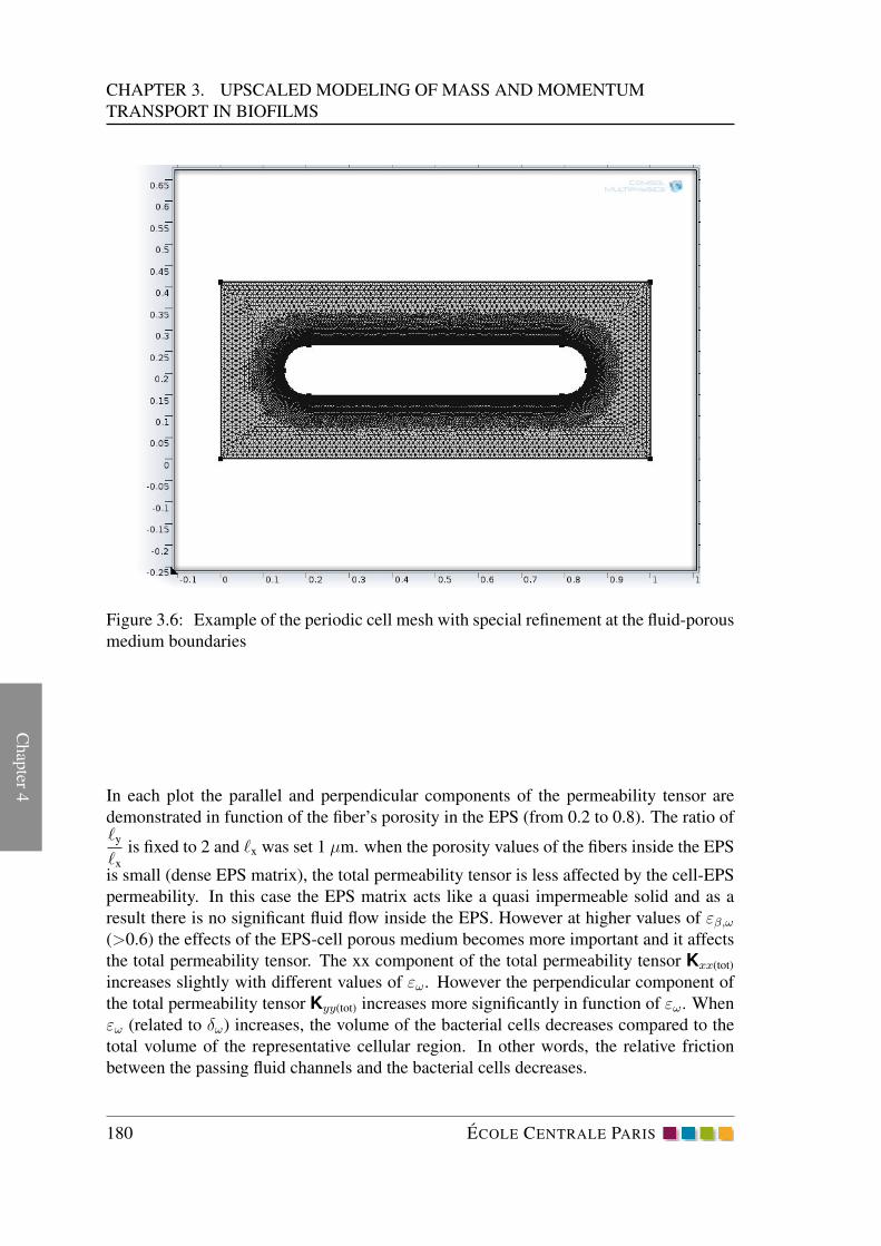
Chap
ter4
CHAPTER 3. UPSCALED MODELING OF MASS AND MOMENTUM
TRANSPORT IN BIOFILMS
Figure 3.6: Example of the periodic cell mesh with special refinement at the fluid-porous
medium boundaries
In each plot the parallel and perpendicular components of the permeability tensor are
demonstrated in function of the fiber’s porosity in the EPS (from 0.2 to 0.8). The ratio ofℓy
ℓx
is fixed to 2 and ℓx was set 1 µm. when the porosity values of the fibers inside the EPS
is small (dense EPS matrix), the total permeability tensor is less affected by the cell-EPS
permeability. In this case the EPS matrix acts like a quasi impermeable solid and as a
result there is no significant fluid flow inside the EPS. However at higher values of εβ,ω(>0.6) the effects of the EPS-cell porous medium becomes more important and it affects
the total permeability tensor. The xx component of the total permeability tensor Kxx(tot)
increases slightly with different values of εω. However the perpendicular component of
the total permeability tensor Kyy(tot) increases more significantly in function of εω. When
εω (related to δω) increases, the volume of the bacterial cells decreases compared to the
total volume of the representative cellular region. In other words, the relative friction
between the passing fluid channels and the bacterial cells decreases.
180 ECOLE CENTRALE PARIS
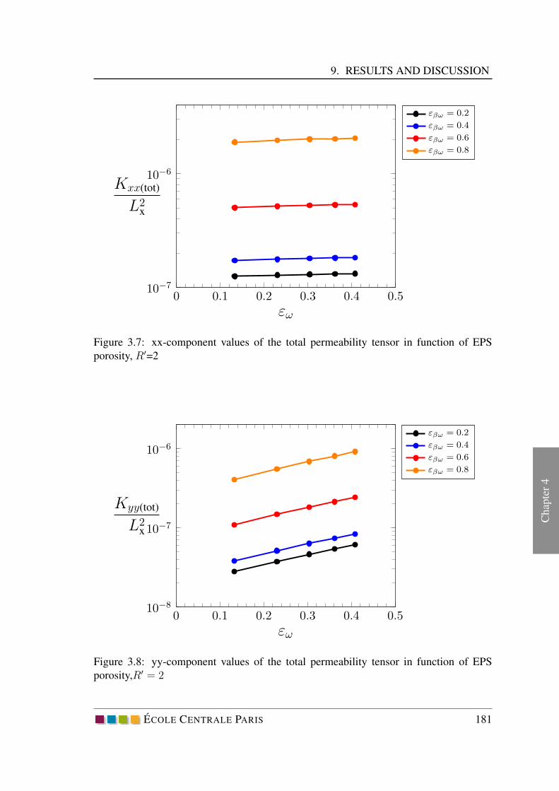
9. RESULTS AND DISCUSSION
Chap
ter
4
0 0.1 0.2 0.3 0.4 0.510−7
10−6
εω
Kxx(tot)
L2x
εβω = 0.2
εβω = 0.4
εβω = 0.6
εβω = 0.8
Figure 3.7: xx-component values of the total permeability tensor in function of EPS
porosity, R′=2
0 0.1 0.2 0.3 0.4 0.510−8
10−7
10−6
εω
Kyy(tot)
L2x
εβω = 0.2
εβω = 0.4
εβω = 0.6
εβω = 0.8
Figure 3.8: yy-component values of the total permeability tensor in function of EPS
porosity,R′ = 2
ECOLE CENTRALE PARIS 181

Chap
ter4
CHAPTER 3. UPSCALED MODELING OF MASS AND MOMENTUM
TRANSPORT IN BIOFILMS
0 2 4 6 8 10 1210−7
10−6
R′
Kxx(tot)
L2x
εβω = 0.2
εβω = 0.4
εβω = 0.6
εβω = 0.8
Figure 3.9: xx-component values of the total permeability tensor in function of R′, δω =5× 10⁻⁷µm
0 2 4 6 8 10 1210−8
10−7
R′
Kyy(tot)
L2x
εβω = 0.2
εβω = 0.4
εβω = 0.6
εβω = 0.8
Figure 3.10: yy-component values of the total permeability tensor in function of R′
(ℓx/ℓy), δω = 5× 10⁻⁷µm
In Fig.3.9 and 3.10, the parallel and perpendicular omponents (xx and yy ) of the total
permeability tensor are presented in function of the relative distance between head-to-
182 ECOLE CENTRALE PARIS

9. RESULTS AND DISCUSSION
Chap
ter
4
head and body-to-body of bacterial arrays. Likewise the first set of results, the significant
effects of the cell-EPS porous interface on the total permeability tensor are more impor-
tant at the higher values of the fibers porosity.
The relative permeability (Kxx
Kyy
) of both total permeability (K) and the biofilm matrix
(Kωσ) are presented in Fig. 3.11-3.14. When porosity of the EPS region (εω) increases,
the relative permeability slightly decreases. This can be reasonable since the resistance
to the flow will reduce in both directions. For variable values of the distance between two
unit cells (R′), when the porosity of fibers is larger than 0.6 (highly hydrated EPS) the par-
allel and perpendicular components of the permeability tensor are more close; however
for more dense structures (εβ,ω ≪ 0.4) evident differences are observed.
0 0.1 0.2 0.3 0.4 0.50
2
4
6
εω
Kxx(tot)
Kyy(tot)
εβω = 0.2
εβω = 0.4
εβω = 0.6
εβω = 0.8
Figure 3.11: Ratio ofKxx(tot)
Kyy(tot)(total permeability tensor) for different values of EPS poros-
ity
ECOLE CENTRALE PARIS 183

Chap
ter4
CHAPTER 3. UPSCALED MODELING OF MASS AND MOMENTUM
TRANSPORT IN BIOFILMS
−2 0 2 4 6 8 10 120
2
4
6
R′
Kxx(tot)
Kyy(tot)
εβω = 0.2
εβω = 0.4
εβω = 0.6
εβω = 0.8
Figure 3.12: Ratio of Kxx
Kyy(total permeability tensor) for different values of R′, δω = 5×
10−7µm
0 0.1 0.2 0.3 0.4 0.5 0.620
30
40
50
εω
Kωσ,xx
Kωσ,yy
εβω = 0.2
εβω = 0.4
εβω = 0.6
εβω = 0.8
Figure 3.13: Ratio ofKωσ,xx
Kωσ,yy(permeability due to EPS-cell porous structure) for different
values of biofilm porosity, R′ = 2
184 ECOLE CENTRALE PARIS
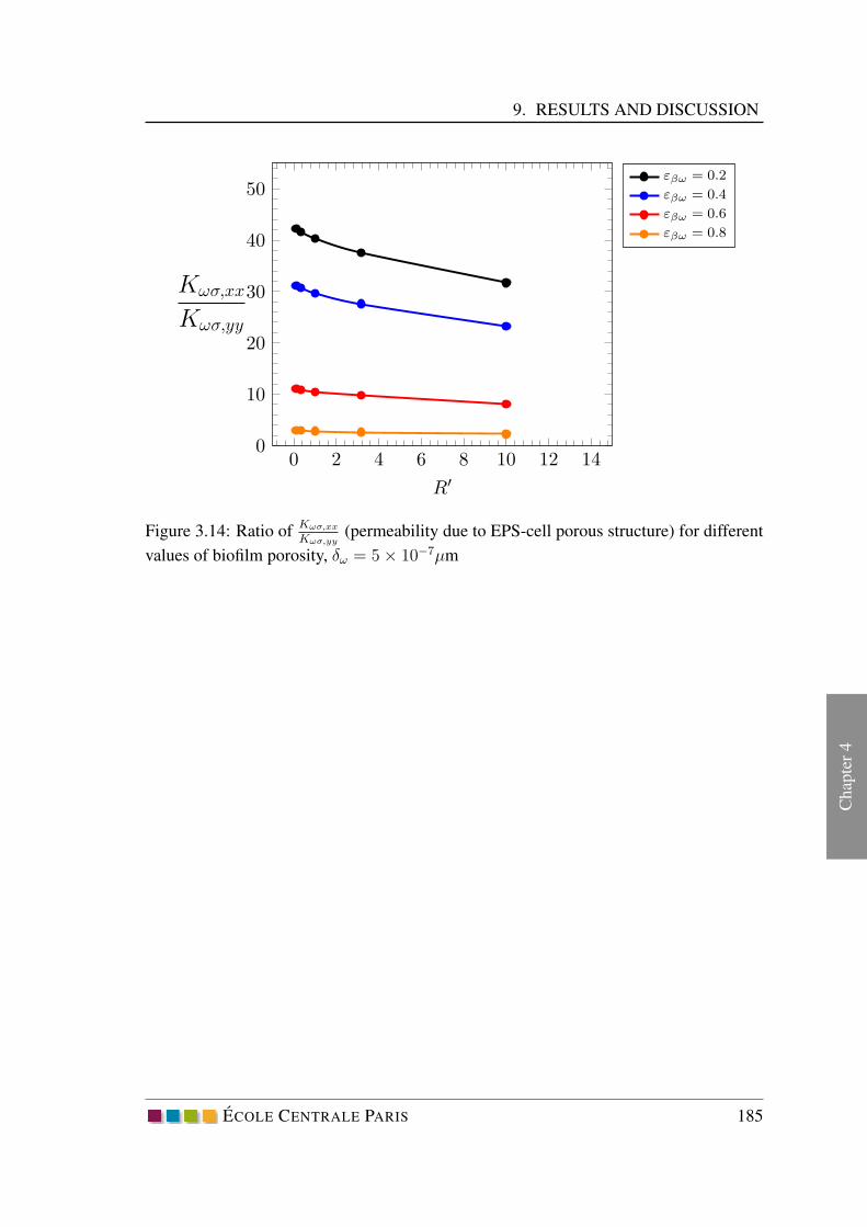
9. RESULTS AND DISCUSSION
Chap
ter
4
0 2 4 6 8 10 12 140
10
20
30
40
50
R′
Kωσ,xx
Kωσ,yy
εβω = 0.2
εβω = 0.4
εβω = 0.6
εβω = 0.8
Figure 3.14: Ratio ofKωσ,xx
Kωσ,yy(permeability due to EPS-cell porous structure) for different
values of biofilm porosity, δω = 5× 10⁻⁷µm
ECOLE CENTRALE PARIS 185

Chap
ter4
CHAPTER 3. UPSCALED MODELING OF MASS AND MOMENTUM
TRANSPORT IN BIOFILMS
10 CONCLUSIONS
Modeling of the porous media involving with biological activity is a challenging task
since it must deal with cellular activity, interfacial mass transport and consequent biomass
production. Moreover, the surrounding environmental conditions (e.g. velocity, solution
chemistry) can highly affect the transport phenomena in the porous media.
In this work, a preliminary biofilm model able to predict the evolution of its structural
properties (porosity, diffusivity) and profiles of velocity and species concentration with
time has been presented. At any point in the biofilm, the structural evolution is due to
transport of chemical species and cellular reaction inside the cells. Three different re-
gions (cells, EPS, water channels) have been identified within the biofilm volume, and
EPS matrix was assumed to be in contact with other regions (no direct contact between
water channels and cells). The model was based on local transport mechanisms involved
with each region, convection and diffusion in ω (EPS) and η (water channels), whereas
only diffusion was taken into account in σ (cells) region. Cellular reaction occurred at
cell-EPS interface and is modeled as function of singles species (glucose) by Michaelis-
Menton kinetics. No reaction took place in EPS and water channels. The mass and mo-
mentum equations, with mass conservation equations for each species at local scale were
given. The upscaled equations have been derived with use of volume averaging method
and associated theorems. The convective averaged velocity fields in η and ω regions
can be determined by the averaged non-stationary stokes equations. In the momentum
transport problem, an equilibrium model and the associated closure problems have been
proposed. the conditions for validation of the equilibrium conditions were presented in
Appendix.B. The upscaled mass conservation equations has been also presented under
the equilibrium conditions. This latter would be required for the numerical simulations
of the macroscopic model (equilibrium concentration field for each species).The porosity
evolution of each region was expressed in function of averaged quantities (concentration,
mass density, velocity). Numerical simulations were run to determine the total permeabil-
ity tensor which depends both on the permeability of the fibers in the EPS (sub scale) and
the permeability due to the biofilm matrix. The results confirmed that in the case of dense
fibers the total permeability tensor is limited by the fibers permeability Kω, however for
loose fibers the permeability of the biofilm matrix Kωσ can play more important role.
This model will be further developed. So far, the biofilm-scale evolution of each region
does not provide data of the overall biomass growth. The final goal is to predict biofilm
structural evolution and heterogeneity by establishing a relation giving the rate of change
of the biofilm thickness as a function of the macroscopic parameters.
186 ECOLE CENTRALE PARIS

GENERAL CONCLUSIONS AND
PERSPECTIVES
ECOLE CENTRALE PARIS 187

Conclu
sion
GENERAL CONCLUSIONS AND PERSPECTIVES
For the past decades, a great interest in using pressure-driven membrane technologies,
as separation techniques, for the design of industrial installations has been rised. They are
used for the purification and separation of different solutions in several industrial fields
(e.g. waste water treatment, food and pharmacy). Compactness and high efficiency of
membrane filtration systems are reported as the main advantages of this technology.
During filtration, solutes and suspended particles with different natures (microorganisms,
natural organic matter, inorganic suspended solids, salts, etc.) accumulate incessantly on
the membrane surface. This results in a(n) (1) flow flux decline, (2) modification of the
membrane properties (selectivity and lifetime) and (3) increase of operational costs. This
phenomenon is called fouling and up to now, represents the main disadvantage of using
membrane technologies. For this reason, different fouling mechanisms (cake formation,
pore constriction, pore blockage) have been studied and models describing each fouling
mechanism have been proposed to get a better understanding of the membrane systems
and to reduce fouling impact.
The objective of this study was to develop a mechanistic understanding of the membrane
fouling developed in the presence of solutions containing bacteria and to propose an up-
scaled model for membrane fouling.
The literature review revealed that during the filtration of liquid media containing micro-
bial cells, the membrane performance is affected by two major factors (1) the irreversible
attachment of the cells to the membrane surface leading to biofilm formation (2) the pen-
etration and blockage of the membrane internal pores by extra cellular products (issued
from the biofilm). Briefly, the biofilm develops an additional dynamic resistance to the
flow at the top of the membrane surface whereas the membrane structure itself, evolves
due to the deposition/adsorption of extracellular polymers produced by the biofilm.
Both porous media (membrane and biofilm) are highly complex and difficult to character-
ize. Moreover, the mechanisms involved in the structural evolution of each porous media
are quite different. The cellular reaction is mainly responsible for biomass production and
subsequent biofilm structural modifications, whereas protein adsorption to the inner pores
affects majorly the membrane structure. All these complexities leaded us to study biofilm
and membrane porous structures separately in order to provide a precise description of
the involving mechanisms on each of them.
Experiments were performed to (1) evaluate the effects of protein adsorption on the mem-
brane system’s performance, (2) characterize the local protein adsorption phenomenon (2)
and (3) determine the structural properties of the original (non-used) membrane (poros-
ity, pore size distribution, permeability, etc.). Experiments provided essential data to the
local model development and will be further used to validate it. The membrane-scale
and biofilm-scale models were both based on the description of the local phenomena at
discontinuous pore scale. The local equations of mass and momentum transport with ap-
propriate boundary conditions (adsorption in the membrane and cellular reaction in the
biofilm) were set. Consequently, the upscaled models were both derived by application of
the volume averaging method and its associated theorems. The upscaled models predicted
in particular the macroscopic evolution of the porous structures (membrane and biofilm)
188 ECOLE CENTRALE PARIS

Concl
usi
on
with time. The effective properties associated with each porous structure (diffusivity and
permeability) were also determined.
It is worth to mention that in both models several simplifications have been made to derive
the closed form of the upscaled equations. These simplifications were mainly based on
the comparison of the order of magnitude of each term or associated length scales. How-
ever, one should keep in mind that numerical calculations of the effective properties and
subsequent comparison of the numerical results with data from experiments are essential
to validate the conditions under which the simplifications are valid.
In the adsorption model, macroscopic numerical simulations were run to validate the
model qualitatively. Due to the tiny size of the membrane active layer, we proposed
to replace this layer with a virtual dividing surface between the fluid phase and porous
medium in which the information about the membrane active layer will be found in the
boundary conditions. It is worth to mention that this kind of jump conditions can be
interesting in other studies as well in order to overcome the pure numerical difficulties.
In the biofilm model, the the local closure problems have been solved numerically in
order to determine the total permeability tensor of the biofilm. The results showed that
the permeability of the fibers inside the EPS matrice has a significant influence on the
permeability tensor. Two different geometries of the representative cellular regions have
been chosen in order to determine their influence on the permeability tensor. When the
thickness of the EPS matrice increases, the fluid has less difficulty to pass though the
bacterial cells in both xx and yy directions and thus the representative region becomes
more permeable.
Some highlights of the models and performed/ongoing experiments will be pointed
out below:
The first model (protein adsorption model) was based on the assumption that when pro-
teins reach the membrane surface they either adsorb to the interface or pass through it.
However experiments confirmed that this hypothesis was only valid for small proteins
where the steric exclusion was negligible. The experiments with BSA solutions clearly
confirmed that the steric hindrance of the large molecules on the membrane surface con-
tributed to the membrane fouling along with adsorption. Consequently in future work, it
would be desirable to develop a coupled model taking into account effects of electrostatic
interaction and particle size on the fouling mechanisms. However the validation of such
models require running direct numerical simulation (DNS) in which particles are deter-
mined to either pass through the membrane or adsorb/block on its surface. This modeling
approach can be subject of future studies in this domain.
Experiments were only carried out with solutions of a single protein in water at pH ∼7. However, it has been remarked by several studies that the solution chemistry (pH and
ionic strength) [75], [116], [167], protein’s mixture (single or binary) [75], [81],[109],
[132], membrane-protein electrostatic/hydrophobic interactions [5], [43], [62], and op-
erational conditions [111], significantly affect protein adsorption both quantitatively and
qualitatively. Therefore experimental sensitivity tests can be performed to (1) determine
ECOLE CENTRALE PARIS 189

Conclu
sion
GENERAL CONCLUSIONS AND PERSPECTIVES
the most important parameters affecting membrane fouling by proteins (2) identify the
underlying mechanisms and (3) further improve the modeling approach.
Recently, confocal scanning laser microscopy (CSLM) has been directly used to ob-
serve the microfiltration membrane performance and to reconstruct the membrane struc-
ture with deposited proteins on it [46],[47], [81], [268]. This approach can be applied
to qualitatively infer the protein deposition/adsorption to the membrane. The amount of
accumulated protein on the membrane surface can be also quantified by FTIR-ATR in
parallel. In future, one can use a combination of these techniques in order to get a more
clear observation of the fouling phenomenon.
The second model (biofilm model) provided the averaged mass and momentum transport
equations in each identified region (Cells, EPS and water channels), with the specific
evolution of their porosity with time. We remind that the porosity evolution was due
to the interfacial mass flux of species and cellular reaction. In future work, a direct
connection between the porosity evolution and the biomass growth at the biofilm scale
will be constructed. The numerical results can be then compared to experimental data.
The upscaled equations for mass conservation of species under the equilibrium conditions
have also been derived. If the local mass equilibrium conditions are valid, one can use
one mass concentration equation for each species in the biofilm volume.
In the biofilm model, information of the biofilm’s structure is absolutely needed to deter-
mine the model parameters (structure, kinetics, transport). For this purpose, experiments
of biofilm formation and development will be carried out with a model bacterium in a
microfiltration membrane system.
Structural parameters of the biofilm can be obtained directly from Confocal Laser Scan-
ning Microscopy (CLSM) image stacks. In fact, CLSM allows non-destructive examina-
tion of biofilms and can be used for their visualization and quantification when combined
with the application of specific staining. In our work, bacteria in the biofilm can be
stained with a specific nucleic acid, and fluorescent labeled lectins, which are specific to
polysaccharides, can be also used. Quantitative parameters describing the physical struc-
ture of biofilms (bio-volumes, porosity, thickness, substratum coverage etc.) can then
be extracted from three-dimensional CLSM images by using appropriate image analysis
software ([38], [100], [267]). Additionally, biofilm permeability can also be measured as
described by [73].
In order to determine the spatial distribution of the different species in the biofilm, micro-
sensors can be used. It has been shown that micro-sensors are useful tools to study
biofilms. They are needle-shaped devices and can quantify the concentration of specific
compounds. Due to their small sensing tip, highly localized measurements are possible
[23].
The first experimental essays will provide parameters to establish the initial conditions
of our model. Thereafter, a sensitivity analysis could be performed in order to determine
the influence of the parameters on the numerical results. One may expect to identify the
parameters that affect biofilm structure significantly and which should be then experi-
mentally measured. Biofilm characterization under different conditions (hydrodynamic,
190 ECOLE CENTRALE PARIS

Concl
usi
on
substrate concentrations. . . ) will also be performed experimentally. Data from these as-
says will then be compared to numerical results for model validation.
The final objective consists of developing a coupled model describing the fouling in the
membrane volume (caused by protein adsorption), and on its surface (biofilm formation)
to predict the overall membrane fouling and its effects on membrane system’s perfor-
mance.
ECOLE CENTRALE PARIS 191


APPENDIX A A
Here we recall the non-closed form of deviation equation of the mass conservation equa-
tion of proteins.
∂cAγ
∂t︸ ︷︷ ︸
Accumulation
− ε−1γ aγκ
∂
∂t[f(〈cAγ〉
γ)]︸ ︷︷ ︸
Adsorptive source
+vγ · ∇cAγ︸ ︷︷ ︸
Convection
+ vγ · ∇ 〈cAγ〉γ
︸ ︷︷ ︸
Convective source
= ∇ · (Dγ∇cAγ)︸ ︷︷ ︸
Diffusion
− ε−1γ ∇ ·
(
Dγ
V
∫
Aγκ
nγκcAγdA
)
︸ ︷︷ ︸
Non-local diffusion
+ ε−1γ ∇ · 〈vγ cAγ〉︸ ︷︷ ︸
Non-local convection
(A.1)
The objective of this part is to make an estimation each term in order to determine the
sources and consequently to propose a closure problem. We begin the process of simpli-
fying Eq. (A.1) by examining the non-local diffusion term
1
V
∫
Aγκ(t)
cAγnγκdA = O (av cAγ) (A.2)
Since we are dealing with an average quantity, we can estimate if the divergence as
∇ ·
{
1
V
∫
Aγκ(t)
cAγnγκdA
}
= O
(av cAγ
L
)
(A.3)
On the basis of Eq. A.3 we estimate the non-local diffusion term in Eq. (A.1) as
ε−1γ Dγ∇ ·
[
1
V
∫
Aγκ(t)
cAγnγκdA
]
= O
(ε−1γ avDγ cAγ
L
)
(A.4)
ECOLE CENTRALE PARIS 193

Appen
dix
APPENDIX A. APPENDIX A
For most porous media, a reasonable representation of the interfacial area per unit volume
is given by
av ≈ ℓ−1γ (A.5)
this leads to the following form of our estimate for the non-local term
ε−1γ Dγ∇ ·
[
1
V
∫
Aγκ(t)
cAγnγκdA
]
= O
(ε−1γ avDγ cAγ
ℓγL
)
(A.6)
while our estimation of the diffusion term in Eq. (A.1) is given by
Dγ∇ · (∇cAγ) = O
(Dγ cAγ
ℓ2γ
)
(A.7)
At this point by use of the length scale constraint ℓγ << L we can discard the diffusive
source likewise.
ε−1γ Dγ∇ ·
[
1
V
∫
Aγκ(t)
cAγnγκdA
]
<< Dγ∇ · (∇cAγ) (A.8)
The order of magnitude of the non-local convective transport term can be expressed
as
ε−1γ ∇ · 〈vγ cAγ〉 = O
(〈vγ〉
γ cAγ
L
)
(A.9)
here we supposed that vγ has the same order of magnitude as 〈vγ〉γ, and we have used L
as the characteristic length associated witht 〈vγ cAγ〉. The order of magnitude of the localconvective transport is given by
vγ · ∇cAγ = O
(〈vγ〉
γ cAγ
ℓγ
)
(A.10)
and this indicates that the non-local convective transport can be neglected when ever
ℓγ << L.
Under these circumstances our transport equation for the spatial deviation concentra-
tion takes the form
∂cAγ
∂t− ε−1
γ aγκ∂
∂t[f(〈cAγ〉
γ)] + vγ · ∇cAγ + vγ · ∇ 〈cAγ〉γ
(A.11)
= Dγ∇ · (∇cAγ)
we can complete the closure problem for cAγ by writing the initial and boundary condi-
tions if we use the spatial deviation decomposition on the interfacial boundary condition
194 ECOLE CENTRALE PARIS

0.
Appen
dix
for cAγ to express
−Dγ∇〈cAγ〉γ · nγκ − Dγ∇cAγ · nγκ =
∂
∂t[f(〈cAγ〉
γ) + f(cAγ)] (A.12)
Now we assume that on the basis of cAγ ≪ 〈cAγ〉γ
the variations of f(cAγ) are negligible
compared to f(〈cAγ〉γ)
B.C.1 − Dγ∇〈cAγ〉γ · nγκ −
∂
∂tf 〈cAγ〉
γ = Dγ∇cAγ · nγκ (A.13a)
It should be noted that the spatial deviation concentration will not, in general, be known
at the entrances and exits of macroscopic system.
B.C.2 cAγ = F(r, t) on Aγe (A.13b)
I.C cAγ = G(r) at t = 0 (A.13c)
While many dispersion processes will be inherently unsteady, the closure problem for cAγ
will be quasi-steady whenever the following constraint is satisfied
Dγt∗
δ2γ>> 1 (A.14)
This constraint is based on the estimation of the diffusive transport term given by
∇ · (Dγ∇cAγ) = O
(Dγ cAγ
δ2γ
)
(A.15)
Where δγ is the characteristic length of the diffusion process along with the inequality
∂cAγ
∂t<< ∇ · (Dγ∇cAγ) (A.16)
when the transport process is purely diffusive, we can conclude that
δγ ≈ ℓγ diffusive process (A.17)
On the other hand when convective transport is important, the situation is more complex.
The qausi-steady closure problem takes the form
vγ · ∇cAγ + vγ · ∇ 〈cAγ〉γ = Dγ∇ · (∇cAγ) (A.18)
ECOLE CENTRALE PARIS 195

Appen
dix
APPENDIX A. APPENDIX A
with boundary conditions
B.C.1 − Dγ∇〈cAγ〉γ · nγκ −
∂
∂t(f 〈cAγ〉
γ) = Dγ∇cAγ · nγκ on Aγκ
(A.19a)
B.C.2 cAγ = F(r, t) on Aγe (A.19b)
it is clear that cAγ will depend on r, t, and ∇ · 〈cAγ〉γ.
We are now in a position to estimate the magnitude of cAγ on the basis of volume and
surface sources. The derivatives of the average concentration are estimated according to
∇〈cAγ〉γ = O
(∆ 〈cAγ〉
γ
L
)
(A.20)
∂
∂tf 〈cAγ〉
γ ≈∂〈cAγ〉
γ
∂tf ′〈cAγ〉
γ = O
[∆ 〈cAγ〉
γ
t∗f ′〈cAγ〉
γ
]
(A.21)
Where t∗ is the characteristic time scale of the adsorption at the membrane scale.
−ε−1γ aγκ
∂
∂t[f(〈cAγ〉
γ)]︸ ︷︷ ︸
Adsorptive source
+vγ · ∇cAγ︸ ︷︷ ︸
Covection
+ vγ · ∇ 〈cAγ〉γ
︸ ︷︷ ︸
Convective source
= Dγ∇ · (∇cAγ)︸ ︷︷ ︸
diffusion
(A.22)
−Dγ∇〈cAγ〉γ · nγκ
︸ ︷︷ ︸
Diffusive source
−∂
∂tf(〈cAγ〉
γ)︸ ︷︷ ︸
Adsorptive source
= Dγ∇cAγ · nγκ on Aγκ
(A.23)
196 ECOLE CENTRALE PARIS

APPENDIX B B
1 LOCAL MASS EQUILIBRIUM
To derive the length-scale constraints, it is convenient to write the closed non-equilibrium
equations as follows
〈ρη〉η
εη
∂εη∂t
+aωηεη
i=5∑
i=1
kηωi (〈ciη〉η −Kηω
eq,i〈ciω〉ω) + 〈ρη〉
η∇ · 〈vη〉η = 0 (B.1a)
〈ρω〉ω
εω
∂εω∂t
+〈ρσ〉
σεσµM
εω
(〈cAσ〉
σ
〈cAσ〉σ +KA
)
−aωηεω
i=5∑
i=1
kηωi (〈ciη〉η −Kηω
eq,i〈ciω〉ω)
+ 〈ρω〉ω∇ · 〈vω〉
ω = 0 (B.1b)
Each average density can be decomposed according to
〈ρη〉η = {ρ}+ εω(〈ρη〉
η − 〈ρω〉ω) (B.2)
〈ρω〉ω = {ρ} − εη(〈ρη〉
η − 〈ρω〉ω) (B.3)
Taking these decomposition into account, we have the following result from subtract-
ing eqs. (B.1)
ECOLE CENTRALE PARIS 197

Appen
dix
APPENDIX B. APPENDIX B
{ρ}
(∂ ln εη∂t
−∂ ln εω∂t
+∇ · (〈vη〉η − 〈vω〉
ω)
)
+ (〈ρη〉η − 〈ρω〉
ω)
(
εω∂ ln εη∂t
+ εη∂ ln εω∂t
+∇ · (εω〈vη〉η + εη〈vω〉
ω
)
+aωηεωηεηεω
i=5∑
i=1
kηωi (〈ciη〉η −Kηω
eq,i〈ciω〉ω)−
〈ρσ〉σεσµM
εω
(〈cAσ〉
σ
〈cAσ〉σ +KA
)
= 0 (B.4)
where, for simplicity we introduced
εωη = εω + εη (B.5)
To make further progress we provide the following orders of magnitude estimates
aωηεωηεηεω
i=5∑
i=1
kηωi (〈ciη〉η −Kηω
eq,i〈ciω〉ω) = O
(εωη
εηεωMaωηk
ωη(〈ρη〉η − 〈ρω〉
ω)
)
(B.6a)
〈ρσ〉σεσµM
εω
(〈cAσ〉
σ
〈cAσ〉σ +KA
)
= O(φ2∇ · 〈vω〉
ω)
(B.6b)
with kωη being an interfacial mass transport coefficient that is on the same order of mag-
nitude as kωηi and φ is a Thiele modulus.
Under these circumstances we may write the following estimates
{ρ} O
(1
t∗+
〈vη〉η − 〈vω〉
ω
L+φ2〈vω〉
ω
L
)
+ (〈ρη〉η − 〈ρω〉
ω) O
(εωt∗
+εηt∗
+εω〈vη〉
η + εη〈vω〉ω
L+φ2εη〈vω〉
ω
L+
kωη
ℓωηM
)
= 0
(B.7)
here we have assumed that t∗η = O(t∗ω) = O(t∗) and that Lη = O(Lω) = O(L). In
addition, we introduced
ℓωη =εωεηεωηaωη
(B.8)
198 ECOLE CENTRALE PARIS

2. CONSTRAINTS FOR NEGLIGIBLE EFFECTS OF THE σ-REGION VELOCITY
Appen
dix
It follows thus,
(〈ρη〉η − 〈ρω〉
ω)
{ρ}
= O
ℓωηL
MLt∗kωη + M(〈vη〉η−〈vω〉ω)
kωη + φ2M〈vω〉ω
kωη
εωℓωηM
kωηt∗+ εηℓωηM
kωηt∗+ ℓωη
L
(εω〈vη〉η+εη〈vω〉ω
kωη/M+ φ2εη〈vω〉ωM
kωη
)
+ 1
(B.9)
Notice that the order of magnitude of the term between square braces in the above esti-
mate is about the unity. This leads us to conclude that under the length-scale constraint
ℓωηL
≪ 1 (B.10)
it is reasonable to assume that
(〈ρη〉η − 〈ρω〉
ω) ≪ {ρ} (B.11)
which is the justification for the local mass equilibrium assumption.
2 CONSTRAINTS FOR NEGLIGIBLE EFFECTS OF THE
σ-REGION VELOCITY
2.1 MASS BALANCE EQUATION IN THE σ-REGION
The objective is to find under which condition the convective effects in Eq. (3.55c) can
be neglected. To do so, the order of magnitude of the time evolution of εσ is needed.
Applying the spatial averaging theorem to the constant quantity 1 in the σ-region leads to
⟨∂1
∂t
⟩
σ
= 0 =∂ 〈1〉σ∂t
−1
V
∫
Aωσ
nσω ·wωσdA (B.12)
and then, with 〈1〉σ = εσ,
∂εσ∂t
= −1
V
∫
Aωσ
nωσ ·wωσdA (B.13)
Remark: the system of equations at intermediate scale is well-posed. nωσ · wωσ could
then be determined numerically, but not literally. Therefore, the surface integral in Eq.
(B.13) cannot be expressed as a function of average quantities. Consequently, it cannot
be used to obtain the time evolution of εσ, which is mandatory for predicting the biofilm
growth.
ECOLE CENTRALE PARIS 199

Appen
dix
APPENDIX B. APPENDIX B
The following order of magnitude can now be deduced
〈ρσ〉σ ∂εσ∂t
= O
(εσ〈ρσ〉
σwωσ
lσ
)
(B.14)
After a comparison with
εσ〈ρσ〉σ∇ · 〈vσ〉
σ = O
(εσ〈ρσ〉
σ〈vσ〉σ
Lvσ
)
(B.15)
Eq. (3.55c) can be simplified into
∂εσ∂t
=1
〈ρσ〉σ1
V
∫
Aωσ
nωσ · ρσ (vσ −wωσ) dA (B.16)
when the following inequality holds
〈vσ〉σ
wωσ
≪Lvσ
ℓσ(B.17)
The velocity in the σ-region should then be at least an order of magnitude higher than the
ω − σ interface velocity.
200 ECOLE CENTRALE PARIS

BIBLIOGRAPHY
[1] Total protein kit, micro lowry, peterson’s modification.
[2] Sethuraman A, Han M, Kane RS, and Belfort G. 18 effect of surface wettability
on the adhesion of proteins. Langmuir, 31(18):7779–7788, 2004.
[3] A.B. Abell, K.L. Willis, and D.A. Lange. Mercury intrusion porosimetry and im-
age analysis of cement-based materials. Journal of Colloid and Interface Science,
211:39–44, 1999.
[4] P. Aimar and P. Bacchin. Slow colloidal aggregation and membrane fouling. Jour-
nal of Membrane Science, 360(1-2):70–76, Sep 2010.
[5] P. Aimar, S. Baklouti, and V. Sanchez. Membrane-solute interactions: Influence on
pure solvent transfer during ultrafiltration. Journal of membrane science, 29:207–
224, 1986.
[6] a.L. Ahmed, K.K. Lau, M.Z. Abu Bakar, and S.R. Abd. Shukor. Integrated cfd
simulation of concentration polarization in narrow membrane channel. Computers
and Chemical Engineering, 29:2087–2095, 2005.
[7] J.D. Andrade, V. Hlady, and A.P. Wei. Adsorption of complex proteins at inter-
faces. Journal of Pure & Appl. Chem., 64(11):1777–1781, 1992.
[8] L. De Angelis and M. M. Fidalgo de Cortalezzi. Ceramic membrane filtration
of organic compounds: Effect of concentration, ph, and mixtures interactions on
fouling. Separation and Purification Technology, 118:762–775, 2013.
[9] B. A. ANNOUS, P. M. FRATAMICO, and J. L. SMITH. Quorum sensing in
biofilms: Why bacteria behave the way they do. Journal of Food Science,
74(1):24–37, 2009.
[10] A. Al Ashhab, M. Herzberg, and O. Gillor. Biofouling of reverse-osmosis mem-
branes during tertiary wastewater desalination: Microbial community composition.
Water Research, 50:341–349, 2014.
ECOLE CENTRALE PARIS 201
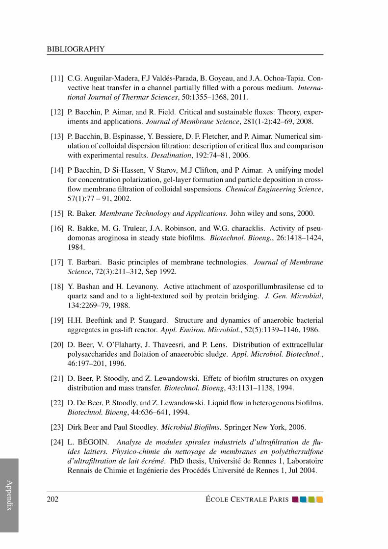
Appen
dix
BIBLIOGRAPHY
[11] C.G. Auguilar-Madera, F.J Valdes-Parada, B. Goyeau, and J.A. Ochoa-Tapia. Con-
vective heat transfer in a channel partially filled with a porous medium. Interna-
tional Journal of Thermar Sciences, 50:1355–1368, 2011.
[12] P. Bacchin, P. Aimar, and R. Field. Critical and sustainable fluxes: Theory, exper-
iments and applications. Journal of Membrane Science, 281(1-2):42–69, 2008.
[13] P. Bacchin, B. Espinasse, Y. Bessiere, D. F. Fletcher, and P. Aimar. Numerical sim-
ulation of colloidal dispersion filtration: description of critical flux and comparison
with experimental results. Desalination, 192:74–81, 2006.
[14] P Bacchin, D Si-Hassen, V Starov, M.J Clifton, and P Aimar. A unifying model
for concentration polarization, gel-layer formation and particle deposition in cross-
flow membrane filtration of colloidal suspensions. Chemical Engineering Science,
57(1):77 – 91, 2002.
[15] R. Baker. Membrane Technology and Applications. John wiley and sons, 2000.
[16] R. Bakke, M. G. Trulear, J.A. Robinson, and W.G. characklis. Activity of pseu-
domonas aroginosa in steady state biofilms. Biotechnol. Bioeng., 26:1418–1424,
1984.
[17] T. Barbari. Basic principles of membrane technologies. Journal of Membrane
Science, 72(3):211–312, Sep 1992.
[18] Y. Bashan and H. Levanony. Active attachment of azosporillumbrasilense cd to
quartz sand and to a light-textured soil by protein bridging. J. Gen. Microbial,
134:2269–79, 1988.
[19] H.H. Beeftink and P. Staugard. Structure and dynamics of anaerobic bacterial
aggregates in gas-lift reactor. Appl. Environ. Microbiol., 52(5):1139–1146, 1986.
[20] D. Beer, V. O’Flaharty, J. Thaveesri, and P. Lens. Distribution of exttracellular
polysaccharides and flotation of anaeerobic sludge. Appl. Microbiol. Biotechnol.,
46:197–201, 1996.
[21] D. Beer, P. Stoodly, and Z. Lewandowski. Effetc of biofilm structures on oxygen
distribution and mass transfer. Biotechnol. Bioeng, 43:1131–1138, 1994.
[22] D. De Beer, P. Stoodly, and Z. Lewandowski. Liquid flow in heterogenous biofilms.
Biotechnol. Bioeng, 44:636–641, 1994.
[23] Dirk Beer and Paul Stoodley. Microbial Biofilms. Springer New York, 2006.
[24] L. BEGOIN. Analyse de modules spirales industriels d’ultrafiltration de flu-
ides laitiers. Physico-chimie du nettoyage de membranes en polyethersulfone
d’ultrafiltration de lait ecreme. PhD thesis, Universite de Rennes 1, Laboratoire
Rennais de Chimie et Ingenierie des Procedes Universite de Rennes 1, Jul 2004.
202 ECOLE CENTRALE PARIS

BIBLIOGRAPHY
Appen
dix
[25] B. Bendinger, H.H.M. Rijnaarts, K. Altendorf, and A.J.B. Zehnder. Physicochem-
ical cell surface and adhesive properties of coryneform bacteria related to the pres-
ence and chain length of mycolic acids. Appl. Environ. Microbiol, 59:3973–77,
1993.
[26] M. Benesse, L.L. Coq, and C. Solliec. Collection efficiency of a woven filter made
of multifiber yarn: Experimental characterization during loading and clean filter
modeling based on a two-tier single fiber approach. ournal of Aerosol Science,
37:974–989, 2006.
[27] R. B. Bird, W. E. Stewart, and E. N. Lightfoot. Transport Phenomena. Wiley, 2nd
edition, 2006.
[28] S. Bottero, Tomas Storck, T. J. Heimovaara, M.C.M. van Loosdrecht, M.V. En-
zienc, and C. Picioreanu. Biofilm development and the dynamics of preferential
flow paths in porous media. Biofouling, 29(9):1069–1086.
[29] P. Bousquet-Melou, B. Goyeau, M. Quintard, F. Fichot, and D. Gobin. Average
momentum equation for interdendritic flow in a solidifying columnar mushy zone.
International Journal of Heat and Mass Transfer, 45(17):3651 – 3665, 2002.
[30] W. R. Bowen and T. A. Doneva. Atomic force microscopy studies of nanofiltration
membranes: surface morphology, pore size distribution and adhesion. Desalina-
tion, 129:163–172, 2000.
[31] W. R. Bowen and Q. Gan. Properties of microfiltration membranes: Adsorption of
bovine serum albumin at polyvinylidene fluoride membranes. Journal of Colloid
and Interface Science, 144(1):254–262, jun 1991.
[32] W. R. Bowen, N. Hilal, R. W. Lovitt, and C. J. Wright. direct measurement of bio-
logical adhesion using an atomic force microscope. Journal of Membrane Science,
154:205–212, 1999.
[33] W.R. Bowen and A. Hermindez J.I. Calvo b. Steps of membrane blocking in flux
decline during protein microfiltration. Journal of Membrane Science, 101:153–
165, 1995.
[34] W.R. Bowen and P.M. Williams. Quantitative predictive modelling of ultrafiltra-
tion processes: colloidal science approaches. Advances in Colloidal Interface,
134/135:3–11, 2007.
[35] Maria G.E.G. Bremer, Jerome Duval, Willem Norde, and Johannes Lyklema. Elec-
trostatic interactions between immunoglobulin (igg) molecules and a charged sor-
bent. Colloids and Surfaces A: Physicochemical and Engineering Aspects, 205(1-
3):29–42, 2004.
ECOLE CENTRALE PARIS 203

Appen
dix
BIBLIOGRAPHY
[36] P. J. Bremer, G.G. Geesey, and B. Drake. Atomic force microscopy examination of
the topography of a hydrated bacterial biofilm on a copper surface. Curr. Microbial,
24:223–230, 1992.
[37] P.J. Bremer, G.G. Geesey, and B. Drake. Atomic force microscopy examination of
the topography of a hydrated bacterial biofilm on a copper surface. Curr. Microbial,
24:223–230, 1992.
[38] A. Bridier, F. Dubois-Brissonnet, A. Bouberta, V. Thomas, and R. Briandet.
The biofilm architecture of sixty opputunistic pathogens deciphered using a hith
throughput clsm method. Journal of Microbial Methods, 82:64–70, 2010.
[39] J.P.F. De Bruijn, F.N. Salazar, and R. Borquez. Membrane blocking in ultrafiltra-
tion: A new approach to fouling. Food and Bioproducts Processing, 83(3):211 –
219, 2005.
[40] J. Bruyers and F. Drummond. Local macromolecule diffusion coefficients in struc-
turally non-uniform bacterial biofilms using fluorescence recovery after photo-
bleaching (frap). Biotechnology and Bioengineering, 60(4):462–473, 1996.
[41] Sz.S. Bucs, A.I. Radu, V. Lavric, J.S. Vrouwenvelder, and C. Picioreanu. Effect
of different commercial feed spacers on biofouling of reverse osmosismembrane
systems: A numerical study. Desalination, 2013.
[42] Burns and Zydney. Effect of solution ph on protein transport through ultrafiltration
membranes. Biotechnol Bioeng, 64(1):27–37, Jul 1999.
[43] A.L. Burns, D.B. Zydney. Contribution to electrostatic interactions on protein
transport in membrane systems. AIChE J., 47(1101), 2001.
[44] R. Chan and V. Chen. Characterization of protein fouling on membranes: oppor-
tunities and challenges. Journal of Membrane Science, 242(1-2):169–188, 2004.
[45] W.G. Characklis, G.A. McFeters, and K.C. Marshall. Physiological ecology in
biofilm systems. John wiley and sons, 1990.
[46] C. Charcosset. Characterization of microporous membrane morphology using con-
focal scanning laser microscopy. Chemical Engineering Science, 55(22):5351–
5358, 2000.
[47] C. Charcosset and J. Bernengo. Comparison of microporous membrane morpholo-
gies using confocal scanning laser microscopy. Journal of Membrane Science,
168(1-2):53–62, 2000.
[48] J. Chayen, L. Bitensky, and R. Butcher. Practical histochemistry. John wiley and
sons, 1973.
204 ECOLE CENTRALE PARIS

BIBLIOGRAPHY
Appen
dix
[49] M. Cheryan. Ultrafiltration and microfiltration handbook. Technomic, Lancaster,
USA, 1998.
[50] R.A.N. Chmielewski and J.F. Frank. Biofilm formation and control in food pro-
cessing facilities. Comprehensive Reviews in Food Science and Food Safety,
2(1):22–32, 2003.
[51] S.W. Choi, J.Y. Yoon, S. Haam, J.K. Jung, J.H. kim, and W.S. Kim. Modeling of
the permeate flux during microfiltration of bsa adsorbed microspheres in a stirred
cell. Journal of Colloid and Interface Science, 228:270–278, 2000.
[52] B.E. Christensen and W.G. Characklis. Physical and chemical properties of
biofilms. W.G. Characklis and K. C. Marshall, john wiley and sons, newyork edi-
tion, 1990.
[53] W. M. Clark, A. Bansal, M. Sontakke, and Y. H. Ma. Protein adsorption and fouling
in ceramic ultrafiltration membranes. Journal of Membrane Science, 55:21–38,
1991.
[54] C.Laspidou, A. Kungolos P., and Samaras. Cellular-automata and individual-based
approaches for the modeling of biofilmstructures: Pros and cons. Desalination,
250:390–394, 2010.
[55] M.M. Cowan, T.M. Waren, and M. Fletcher. Mixed species colonization of solid
surfaces in labratory biofilms. Biofouling, 3:23–34, 1991.
[56] Z. Cui. Protein separation using ultrafiltration — an example of multi-scale com-
plex systems. China Particuology, 3(6):343–348, 2005.
[57] Monroe D. ) looking for chinks in the armor of bacterial biofilms. PLoS. Biol,
5(11), Monroe D.
[58] A. Danielsson, B. Norkrans, and A. Bjornsson. On bacterial adhesion-the effect of
certain enzymes on adhered cells in a marine pseudomonasspecies. Bot. Marina,
20:7–13, 1977.
[59] D.G. Davies, M.R. Parsek, J.P. Pearson, B.H. Iglewski, J.W. Costerton, and E.P.
Greenberg. The involvement of cell-to-cell signals in the development of a bacte-
rial biofilm. Science, 289:295–298, 1998.
[60] Y. Davit. Multiple-scale analysis of transport phenomena in porous media with
biofilms. PhD thesis, Universite de Toulouse, 2010.
[61] C. D. de Gooijer, R. H. Wijffels, and J. Tramper. Growth and substrate consump-
tion of nitrobacter agilis cells immobilized in carrageenan: Part 1. dynamic mod-
eling. Biotechnol. Bioeng., 38(224-231), 1991.
ECOLE CENTRALE PARIS 205

Appen
dix
BIBLIOGRAPHY
[62] Emilio J. de la Casa, Antonio Guadix, Ruben Ibanez, Fernando Camacho, and
Emilia M. Guadix. A combined fouling model to describe the influence of the
electrostatic environment on the cross-flow microfiltration of {BSA}. Journal of
Membrane Science, 318(1–2):247 – 254, 2008.
[63] C. de M. Coutinho, M. C. Chiu, R. C. Basso, A. P. B. Ribeiro, L. A. G. Goncalves,
and L. A. Viotto. State of art of the application of membrane technology to veg-
etable oils: A review. Food Research International, 42(5-6):536–550, 2009.
[64] A.L. Decho. Exopolymer microenvironments of microbial flora: multiple and in-
teractive effects on trophic relationships. Role of bacterial exopolymeric capsules
in Limnol. Oceanogr., 38(8):1633–1645, 1993.
[65] D. Delaunay. Nettoyage eco-efficace de membranes planes et spirales
d’ultrafiltration de lait ecreme Approches physico-chimiques et hydrodynamiques
concertees. PhD thesis, L’UNIVERSITE DE RENNES 1, 2007.
[66] David Delaunay, Murielle Rabiller-Baudry, Jose M. Gozalvez-Zafrilla, Beatrice
Balannec, Matthieu Frappart, and Lydie Paugam. Mapping of protein fouling
by ftir-atr as experimental tool to study membrane fouling and fluid velocity
profile in various geometries and validation by {CFD} simulation. Chemical
Engineering and Processing: Process Intensification, 47(7):1106 – 1117, 2008.
¡ce:title¿Euromembrane 2006¡/ce:title¿.
[67] S. M. Ghasemi Demneh, B. Nasernejad, and H. Modarres. Modeling investiga-
tion of membrane biofouling phenomena by considering the adsorption of protein,
polysaccharide and humic acid. Colloids and Surfaces B: Biointerfaces, 88:108–
114, 2011.
[68] Q. Derekx, P. Bacchin, D. Veyret, K. Glucina, and P. Moulin. Simulation of particle
capture in a microfiltration membrane. Water Science Technology, 64(6):1368–73,
2011.
[69] d.G. Green. Cellular automata models in biology. Math. Comp. Mod, 13:69–74,
1990.
[70] R. M. Donlan and J. W. Costerton. Biofilms: Survival mechanisms of clinically
relevant microorganisms. Clinical Microbiology Review, 15(2):167–193, 2002.
[71] R.M. Donlan. Biofilms: Microbial life on surfaces. Emerging Infectious Deseases,
8(9):881–889, Sep 2004.
[72] R.M. Donlan, W.O. Pipes, and T.L. Yohe. Biofilm fomation on cast iron substrata
in water distribution systems. Water Res, 28:1497–1503, 1994.
206 ECOLE CENTRALE PARIS

BIBLIOGRAPHY
Appen
dix
[73] C. Dreszer, H.C. Flemming, A. Zwijnenburg, J.C. Kruithof, and
J.S.Vrouwenvelder. Impact of biofilm accumulation on transmembrane and
feed channel pressure drop: effects of crossflow velocity, feed spacer and
biodegradable nutrient. Water Research, 2013.
[74] Chase Duclos-Orsello, Weiyi Li, and Chia-Chi Ho. A three mechanism model
to describe fouling of microfiltration membranes. Journal of Membrane Science,
280(1–2):856 – 866, 2006.
[75] Ulla M. Elofsson, Marie A. Paulsson, and Thomas Arnebrant. Adsorption of -
lactoglobulin a and b: Effects of ionic strength and phosphate ions. Colloids and
Surfaces B: Biointerfaces, 8(3):163 – 169, 1997.
[76] B. Espinasse, P. Bacchin, and P. Aimar. Filtration method characterizing the re-
versibility of colloidal fouling layers at a membrane surface. Journal of colloid
and interface science, 320(2):483–490, 2008.
[77] Frank B. F. and Belfort G. Atomic force microscopy for low adhesion surfaces:
Thermodynamic criteria, critical surface tension and intermolecular forces. Lang-
muir, 17(6):1905–1912, 2001.
[78] S. Fakhfakh, S. Baklouti, S. Baklouti, and J. Bouaziz. characterization and appli-
cation in bsa solution of silica ceramic membranes. Desalination, 262:188–195,
2010.
[79] A.G. Fane, C.J.D. Fell, and A. Suki. The effect of ph and ionic environment on the
ultrafiltration of protein solutions with retentive membranes. Journal of Membrane
Science, 195-210, 1983.
[80] P. Fera, M.A. Siebel, W.G., and D. Prieur. Seasonal variations in bacterial colo-
nization of stainless steel, aluminium, and polycarbonate surfaces is seawater flow
system. Biofouling, 1:251–61, 1989.
[81] M. Ferrando, A. Rozek, M. Zator, F. Lopez, and C. Guell. An approach to
membrane fouling characterization by confocal scanning laser microscopy. 2005,
250(1-2):283–293, Mar Journal of Membrane Science.
[82] M. Fletcher. The application of interface reflection microscopy to the study of
vacterial adhesion to solid surfaces. Elsevier applied science, 1988.
[83] M. Fletcher. Attachment of pseudomonas fluorescens to glass and influence of
electrolytes on bacterium-substratum separation distance. J Bacteriol, 170:2027–
30, 1988.
[84] M. Fletcher and G.I. Leob. Influence of substratum characterization on the at-
tachment of a marine pseudomonad to solid surfaces. Appl. Environ. Microbiol,
37:67–72, 1979.
ECOLE CENTRALE PARIS 207

Appen
dix
BIBLIOGRAPHY
[85] A. Fouladitajar, F. Zokaee Ashtiani, A. Okhovat, and B. Dabir. Membrane fouling
in microfiltration of oil-in-water emulsions; a comparison between constant pres-
sure blocking laws and genetic programming (gp) model. Desalination, 329:41–
49, 2013.
[86] J.D. Fowler and C.R. Robertson. Hydraulic permeability of immobilized bacterial
cell aggregates. Appl. Environ. Microbiol, 57(1):102–113, 1991.
[87] H. Fujikawa and M. Matsushita. Fractal growth of bacillus subtilis on agar plates.
J. Phys. Soc. Jpn., 58:3875–3878, 1989.
[88] Hiroshi Fujikawa. Diversity of the growth patterns of bacillus subtilis colonies on
agar plates. {FEMS} Microbiology Ecology, 13(3):159 – 167, 1994.
[89] S. Fukuzaki, H. Urano, and K. Nagata. Adsorption of bovine serum albumin onto
metal oxide surfaces. Journal of Fermentation and Bioengineering, 81:163–167,
1996.
[90] F. Golfier, B. D. Wood, L. Orgogozo, and M. Bues M. Quintard. Biofilms in
porous media: development of macroscopic transport equations via volume av-
eraging with closure for local mass equilibrium conditions. Advances in water
resources, 32:463–485, 2009.
[91] W.G. Gray. A derivations of the equations for multiphase transport. Chemical
Engineering Sciences, 30:229–233, 1975.
[92] T. Griebe and H. C. Flemming. Biocide-free antifouling strategy to protect ro
membranes from biofouling. Desalination, 118:153–157, 1998.
[93] P.A. Gunning, A.B. Kirby, M.L. Parker, A.P. Gunning, and V.J. Morris. Com-
parative imaging of pseudomonas putida bacterial biofilms by scannig electrom
microscopy and both dc contact and ac non-contact atomic force microscopy. J.
Appl. Bacteriol, 81(3):276–282, 1996.
[94] M. Hasanizadeh and W.G. Gray. General conservation equations for multi-phase
systems: 1. averaging procedure. Advance in water resources, 2:131–144, 1979.
[95] M. Hashinoa, K. Hiramia, T. Ishigamia, Y. Ohmukaia, T. Maruyamaa, N. Kubotab,
and H. Matsuyamaa. Effect of kinds of membrane materials on membrane fouling
with bsa. Journal of Membrane Science, 384:157–165, 2001.
[96] S. J. Haward, P. R. Shewry, M. J. Miles, and T. J. Mcmaster. Direct real-time imag-
ing of protein adsorption onto hydrophilic and hydrophobic surfaces. Biopolymers,
93(1):74–84, 2010.
208 ECOLE CENTRALE PARIS

BIBLIOGRAPHY
Appen
dix
[97] Charles A. Haynes, Edward Sliwinsky, and Willem Norde. Structural and electro-
static properties of globular proteins at a polystyrene-water interface. Journal of
Colloid and Interface Science, 164(2):394 – 409, 1994.
[98] J. Hermia. Constant pressure blocking filtration laws, application to power-law
non-newtonian fluids. Trans IChemE, 60, 1982.
[99] C. HERRERO, P. Pradanos, J. I. Calvio, F. Tejerina, and A. Hernandez. Flux
decline in protein microfiltration: Influence of operative parameters. Journal of
Colloid and Interface Science, 187:344–355, May 1996.
[100] A. Heydorn, A. T. Nielsen, M. Hentzer, C. Sternberg, M. Givskov, B. K. Ersbøll,
and S. Molin. Quantification of biofilm structures by the novel computer program
comstat. Microbiology (2000), 146,, 146:2395–2407, 2000.
[101] N. Hilal, A. W. Mohammad, B. Atkin, and N. A. Darwish. Using atomic force
microscopy towards improvement in nanofiltration membranes properties for de-
salination pre-treatment: a review. Desalination, 157:137–144, 2003.
[102] Chia-Chi Ho and A. L. Zydney. A combined pore blockage and cake filtration
model for protein fouling during microfiltration. Journal of Colloid and Interface
Science, 232(2):389–399, 2000.
[103] Chia-Chi Ho and Andrew L. Zydney. A combined pore blockage and cake filtration
model for protein fouling during microfiltration. Journal of Colloid and Interface
Science, 232(2):389 – 399, 2000.
[104] W. H. Howard and R. Lambert. Ultrafiltration in the ontario dairy industry. Cana-
dian Journal of Agricultural Economics, 41(2):177–195, 1993.
[105] F.A. Howes and S. Whitaker. The spatial averaging theorem revisited. Chemical
Engineering Science, 40:1387–1392, 1985.
[106] K M Hsieh, G A Murgel, L W Lion, and M L Shuler. Interactions of micro-
bial biofilms with toxic trace metals: 2. prediction and verification of an inte-
grated computer model of lead (ii) distribution in the presence of microbial activity.
Biotechnol Bioeng, 44(2):232–9, Jun 1994.
[107] L. Huang and M.T. Morrissey. Finite elements analysis as a tool for cross flow
membrane filter simulation. Journal of Membrane Science, 15(:19–30, 1999.
[108] I. H. Huisman and A. Hernandez P. Pradanos. The effect of protein-protein and
protein-membrane interactions on membrane fouling in ultrafiltration. Journal of
Membrane Science, 179(79), 2000.
ECOLE CENTRALE PARIS 209

Appen
dix
BIBLIOGRAPHY
[109] Kuo-Jen Hwang and Pan-Yu Sz. Filtration characteristics and membrane fouling in
cross-flow microfiltration of bsa/dextran binary suspension. Journal of Membrane
Science, 347:75–82, 2010.
[110] Kuo-Jen Hwang and Pan-Yu Sz. Effect of membrane pore size on the performance
of cross-flow microfiltration of bsa/dextran mixtures. Journal of Membrane Sci-
ence, 378:272–279, 2011.
[111] Kuo-Jen Hwang and Pan-Yu Sz. Membrane fouling mechanism and concentration
effect in cross-flow microfiltration of bsa/dextran mixtures. Chemical Engineering
Journal, 166:669–677, 2011.
[112] J. Jacob, P. Pradanos, J.I. Calvo, A. Hernandez, and G. Jonsson. Fouling kinetics
and associated dynamics of structural modifications. Colloids and Surfaces A:
Physicochemical and Engineering Aspects, 138:173–183, 1998.
[113] B. Jiaoa, A. Cassano, and E. Driolib. Recent advances on membrane processes for
the concentration of fruit juices: a review. Journal of Fod Engineering, 63(3):303–
324, 2004.
[114] R. Jiraratananon, D. Uttapap, and P. Samprranpibon. Cross-flow microfiltration of
a colloidal suspension with the presence of macromolecules. Journal of Membrane
Science, 140:57–66, 1998.
[115] K. L. Jones and C. R. O’Melia. Ultrafiltration of protein and humic substances:
effect of solution chemistry on fouling and flux decline. Journal of Membrane
Science, 193(2):163–173, 2001.
[116] Kimberly L. jones and charles R. O’melia. Protein and humic acid adsorption
onti hydrophilic membrane surfaces: effects of ph anf ionic strength. Journal of
Membrane Science, 165:31–46, 2000.
[117] B.B. Jørgensen. Diffusion processes and boundary layers in microbial mats. Mi-
crobial Mats, 35(243-253), 1994.
[118] B.B. Jørgensen and D;J. Des Marais. The diffusive boundary layer of sediments:
oxygen microgradients over a microbial mat. Limnol Oceanogr, 35(6):1343–55,
1990.
[119] D. M. Kanani, X. Sun, , and R. Ghosh. Membrane fouling during microfiltration
of protein solutions. Journal of Membrane science, 315(1-2):219, 2008.
[120] Seok-Tae Kang, E. M.V. Hoek Arun Subramani, M. A. Deshusses, and M. R. Mat-
sumoto. Direct observation of biofouling in cross-flow microfiltration: mecha-
nisms of deposition and release. Journal of Membrane Science, 244:151–165,
2004.
210 ECOLE CENTRALE PARIS

BIBLIOGRAPHY
Appen
dix
[121] G.E. Kapellos, T.S. Alexiou, and A.C. Payatakes. Hierarchical simulator of biofilm
growth and dynamics in granular porous materials. Advances in Watater resources,
30:1648–1667, 2007.
[122] George E. Kapellos, Terpischori S. Alexiou, and Alkiviades C. Payatakes. a mul-
tiscale theoritical model for fluid flow in cellular biological media. International
journal of engineering science, 51:241–271, 2012.
[123] M.C. Kaplan, A. Jegou, B. Chaufer, M. Rabiller-Baudry, and M.C. Michalsky. Ad-
sorption of lysozyme on membrane material and cleaning with non ionic surfactant
characterised through contact angle measurements. Desalination, 146:149–154,
2002.
[124] Martin Karlsson and Uno Carlsson. Protein adsorption orientation in the light of
fluorescent probes: Mapping of the interaction between site-directly labeled human
carbonic anhydrase {II} and silica nanoparticles. Biophysical Journal, 88(5):3536
– 3544, 2005.
[125] S.T. kelly, W.S. Opong, and A.L. Zydney. The influence of protein aggregation on
the fouling of microfiltration membranes during stirred cell filtration. Journal of
Membrane Science, 80(1-2):175–187, 1993.
[126] S.C. Kim, R. Sprung, Y. Chen, Y. Xu, H. Ball, J. Pei, T. Cheng, Y. Kho, H. Xiao,
L. Xiao, N.V. Grishin, M. White, X. J.Yang, and Y. Zhao. Substrate and functional
diversity of lysine acetylation revealed by a proteomics survey. Molecular Cell,
23(4):607–618, 2006.
[127] J.C. Kissel, P.L. Mccarty, and R.L. Street. Numerical-simulation of mixed-culture
biofilm. J. Environ. Eng, 110:393–411, 1984.
[128] B. V. KJELLERUP, T. R. THOMSEN, J. L. NIELSEN, B. H. OLESEN,
B. FRØLUND, and P. H. NIELSEN. Microbial diversity in biofilms from cor-
roding heating systems. Biofouling, 21(1):19–29, 2005.
[129] M. K. Ko, K. D. Caleb, and J. Pellegrino. Determination of total protein adsorbed
on solid (membrane) surface by a hydrolysis technique: single protein adsorption.
Journal of Membrane Science, 93:21–30, 1994.
[130] J. A. Koehler, M. Ulbricht, and G. Belfort. Intermolecular forces between proteins
and polymer films with relevance to filtration. Langmuir, 13(15):4162–4171, 1997.
[131] J. A. Koehler, M. Ulbricht, and G. Belfort. Intermolecular forces between a pro-
tein and a hydrophillic polysulfone film with relevance to filtration. Langmuir,
16:10419–10427, 2000.
ECOLE CENTRALE PARIS 211

Appen
dix
BIBLIOGRAPHY
[132] K. Konttufi and M. Vuofisto. Adsorption of globular proteins on polymeric micro-
filtrafion membranes. Desalination, 104:99–105, 1996.
[133] D.R. korber, J.R. Lawrence, B. Sutton, and D.E. Caldwell. Effect of lami-
nar flow velocity on the kinetics of surface recolonization by mot+ and mot−
pseudomonasfluoroscens. Microb. Ecol, 18:1–19, 1989.
[134] R. Krishna and J. A. Wesselingh. The maxwell-stefan approach to mass transfer.
Chemical Engineering Science, 52(6):861–911, 1997.
[135] l. Zeman and A.L. Zydney. Microfiltration and ultrafiltration: Principles and
applications. Marcel Dekker, Newyork, 1996.
[136] I. Langmuir. Vapor pressures, evaporation, condensation and adsorption. J. Am.
Chem. Soc, 54(7):2798–2832, 1932.
[137] P. Lauger. Carrier-mediated ion transport. Science, 178:24–30, 1972.
[138] P. Lauger, R. Benz, G. Stark, E. Bamberg, P. C. Jordan, A. Fahr, and W. Brock.
Relaxation studies of ion transport systems in lipid bilayer membranes. Quarterly
Reviews of Biophysics, 14:513–598, 1981.
[139] J.R. Lawrence, D.R. Korber, B.D. Hoyle, J.W. Costerton, and D.E. Caldwell. Op-
tical sectioning of microbial biofilms. J. Bacteriol, 173(20):6558–6567, 1991.
[140] J. Li, R.D. Sanderson, G.Y. Chai, and D.K. Hallbauer. Development of an ultra-
sonic technique for in situ investigating the properties of deposited protein during
crossflow ultrafiltration. Journal of Colloid and Interface Science, 284:228–238,
2005.
[141] X. Li, Y. Zhang, and X. Fu. Adsorption of glutamicum onto polysulphone mem-
brane. Separation and Purification Technology, 37:187–198, 2004.
[142] Xiufen Li, Yushan Zhang, and Xueqi Fuc. Adsorption of glutamicum onto poly-
sulphone membrane. Separation and Purification Technology, 37:187–198, 2004.
[143] B. Little, P. Wagner, R.Ray, R. Pope, and R. Scheetz. Biofilms, an esem evaluation
of artifacts introduced during preperation. J. Ind. Microbiol., 8(4):213–222, 1991.
[144] G.I. Loeb and R.A. Neihof. Marine conditioning films. Advances in chemistry,
145:319–35, 1975.
[145] F.A. Lopes, P. Morin, R. Oliveira, and L. F. Melo. Interaction of desulfovib-
rio desulfuricans biofilms with stainless steel surface and its impact on bacterial
metabolism. Journal of Applied Microbiology, 101:1087–1095, 2006.
212 ECOLE CENTRALE PARIS

BIBLIOGRAPHY
Appen
dix
[146] F.A. Lopes, P. Morin, R. Oliveira, and L.F. Melo. Impact of biofilms in simulated
drinking water and urban heat supply systems. International Journal of Envioron-
mental Engineering, 1(3):276–294, 2009.
[147] D. Lopez, H. Vlamakis, and R. Kolter. Biofilms. Cold Spring Harbor Perspectives
in Biology, 2(7), 2010.
[148] Levia Lopez. Ultrafiltration in rotary annular flow. PhD thesis, Land university,
Sweden, 1979.
[149] Livia Lopez and E Mathiasson. Solute adsorption as a source of fouling in ultrafil-
tration. Land university press, Sweden, pages 299–308, 1981.
[150] Rabe M, Verdes D, Rankl M, Artus GR, and Seeger S. A comprehensive study
of concepts and phenomena of the nonspecific adsorption of β-lactoglobulin.
Chemphyschem, 23(8):862–876, 2007.
[151] F. Macedonio, E. Drioli, A. A. Gusev, A. Bardow, R. Semiat, , and M. Kurihara.
Efficient technologies for worldwide clean water supply. hemical Engineering and
Processing, 51:2–17, Jan 2012.
[152] Z. Mai. Membrane processes for water and wastewater treatment: study and mod-
eling of interactions between membrane and organic matter. PhD thesis, Ecole
Centrale Paris, 2013.
[153] Martin Malmsten. Formation of adsorbed protein layers. Journal of Colloid and
Interface Science, 207(2):186–199, 1998.
[154] S.S. Manickam, J. Gelb, and J.R. McCutcheon. Pore structure characterization of
asymmetric membranes: Non-destructive characterization of porosity and tortuos-
ity. Journal of Membrane Science, 2014.
[155] S.S. Manickam and J.R. McCutcheon. Characterization of polymeric nonwovens
using porosimetry, porometry and x-ray computed tomography. Journal of Mem-
brane Science, 407-408:108–115, 2012.
[156] Bernard Marcos, Christine Moresolib, Jana Skorepovab, and Brandi Vaughanb.
Cfd modeling of a transient hollow fiber ultrafiltration system for protein concen-
tration. Journal of Membrane Science, 337:136–144, 2009.
[157] A.D. Marshall, P.A. Munro, and G. Tragardh. The effect of protein fouling in
microfiltration and ultrafiltration or permeate flux, protein retention and selectivity:
a literature review. Desalination, 65(1):91, 1993.
[158] K.C. Marshall, R. Stout, and R. Mitchell. Mechanisms of the initial events in the
sorption of marine bacteria to surfaces. J. Gen. Microbial, 68:337–48, 1971.
ECOLE CENTRALE PARIS 213

Appen
dix
BIBLIOGRAPHY
[159] F. Martinez, A. Martin, P. Pradanos, J.I. Calvo, L. Palacio, and A. Hernandez.
Protein adsorption and deposition onto microfiltration membranes: The role of
solute-solid interactions. Journal of Colloid and Interface Science, 221:254–261,
2000.
[160] E. Matiasson. The role of macromolecular adsorption in fouling of ultrafiltration
membranes. Journal of membrane science, 16:23–36, 1983.
[161] M. Matsushita and H. Fujikawa. Diffusion-limited growth in bacterial colony for-
mation. Physica A, 168:498–506, 1990.
[162] E. Matthiasson. The role of macromolecular adsorption in fouling of ultrafiltration
membranes. Journal of Membrane Science, 16:23–36, 1983.
[163] R. Mcdonogh, G. Schaule, and H.C. Flemming. The permeability of biofouling
layers on membranes. Journal of Membrane Science, 87:199–217, 1994.
[164] J. McGuire, V. Krisdhasima, Marie C. Wahlgren, and Thomas Arnebrant. Compar-
ative Adsorption Studies with Synthetic, Structural Stability and Charge Mutants
of Bacteriophage T4 Lysozyme. American Chemical Society, 1995.
[165] Joseph McGuire, Marie C. Wahlgren, and Thomas Arnebrant. Structural stabil-
ity effects on the adsorption and dodecyltrimethylammonium bromide-mediated
elutability of bacteriophage {T4} lysozyme at silica surfaces. Journal of Colloid
and Interface Science, 170(1):182 – 192, 1995.
[166] M K Menon and A L Zydney. Effect of ion binding on protein transport through
ultrafiltration membranes. Biotechnol Bioeng, 63(3):298–307, May 1999.
[167] H. Mo, K.G. Tay, and H.Y. Ng. Fouling of reverse osmosis membrane by protein
(bsa): Effects of ph, calcium, magnesium, ionic strength and temperature. Journal
of Membrane Science, 31:28–35, 2008.
[168] Huajuan Mo, Kwee Guan Tay, and How Yong Ng. Fouling of reverse osmosis
membrane by protein (bsa): Effects of ph, calcium, magnesium, ionic strength and
temperature. Journal of Membrane Science, 315:28–35, 2008.
[169] S. Mochizuki and A.L. Zydney. Sieving characteristics of albumin deposits formed
during microfiltration. Journal of Membrane Science, 158(1):136–145, Jun 1993.
[170] K. Monkos. Viscosity of bovine serum albumin aqueous solutions as a function
of temperature and concentration. International Journal of Biological Macro-
molecules, 18(1-2):61–68, 1996.
214 ECOLE CENTRALE PARIS

BIBLIOGRAPHY
Appen
dix
[171] E. Morin-Couallier, C. Fargues, R. Lewandowski, M. Decloux, and M.L.
Lameloise. Reducing water consumption in beet distilleries by recycling the con-
densates to the fermentation phase. Journal of Cleaner Production, 16:655–663,
2008.
[172] S. Mortazavi. Application of Membrane Separation Technology to Mitigation of
Mine Effluent and Acidic Drainage. Natural Resources Canada, 2008.
[173] M. J. Munoz-Aguado, D. E. Wiley, and A. G. Fane. Enzymatic and detergent clean-
ing of a polysulfone ultrafiltration membrane fouled with bsa and whey. Journal
of Membrane Science, 117:175–187, 1996.
[174] A. Nabe, E. Staude, and G. Belfort. Surface modification of polysulfone ultrafil-
tration membranes and fouling by bsa solutions. Journal of Membrane Science,
133:57–72, 1997.
[175] K. Nakamura and K. Matsumoto. Adsorption behavior of bsa in microfiltration
with porous glass membrane. Journal of Membrane Science, 145:119–128, 1998.
[176] K. Nakamura and K. Matsumoto. Properties of protein adsorption onto pore sur-
face during microfiltration: Effects of solution environment and membrane hy-
drophobicity. Journal of Membrane Science, 280:363–374, 2006.
[177] K. Nakamura and K. Matsumoto. rotein adsorption properties on a microfiltra-
tion membrane: A comparison between static and dynamic adsorption methods.
Journal of Membrane Science, 285:126–136, 2006.
[178] K. Nakanishi, T. Sakiyama, and K. Imamura. On the adsorption of proteins on
solid surfaces, a common but very complicated phenomenon. Journal of Biosience
and Bioengineering, 91(3):233–244, 2001.
[179] T. Neu and J.R. Lawrence. Development and structure of microbial biofilms in
river water studied by confocal laser scanning microscopy. FEMS Microbial. Ecol,
24:11–25, 1997.
[180] J.L. Nilsson. Fouling of an ultrafiltration membrane by a dissolved whey protein
concentrate and some whey proteins. Journal of Membrane Science, 36:147–160,
1988.
[181] Willem Norde. Driving forces for protein adsorption at solid surfaces. Macro-
molecular Symposia, 103(1):5–18, 1996.
[182] Willem Norde. My voyage of discovery to proteins in flatland and beyond. Colloids
and Surfaces B: Biointerfaces, 61(1):1 – 9, 2008.
ECOLE CENTRALE PARIS 215

Appen
dix
BIBLIOGRAPHY
[183] Willem Norde and Carla E Giacomelli. Bsa structural changes during homomolec-
ular exchange between the adsorbed and the dissolved states. Journal of Biotech-
nology, 79(3):259 – 268, 2000.
[184] M. Nystrom. Fouling of unmodified and modified polysulfone ultrafiltration mem-
branes by ovalbumin. Journal of Membrane Science, 44:183–196, 1989.
[185] J.A. Ochoa-Tapia, J.A. del Rıo, and S. Whitaker. Bulk and surface diffusion in
porous media, an application of the surface-averaging theorem. Chemical Engi-
neering Science, 48(11):2061–2082, 1993.
[186] W.S. Opong and A.L. Zydney. Hydraulic permeability of protein layers deposited
during ultrafiltration. Journal of Colloid and Interface Science, 142:41, 1991.
[187] S.F. Oppenheim, C.B. Phillips, and V.G.J. Rodgers. Analysis of initial protein
surface coverage on fouled ultrafiltration membranes. Journal of Colloid and In-
terface Science, 184:639–651, 1996.
[188] L. Orgozozo, F. Golfier, M. Bues, and M. Quintard. Upscaling of transport process
in porous media with biofilms in non-equilibrim conditions. Advance in water
resources, 33:585–600, 2010.
[189] L. Palacio, C.-C. Hob, P. Pradanos, A. Hernandez, and A.L. Zydney. Fouling
with protein mixtures in microfiltration: Bsa–lysozyme and bsa–pepsin. Journal
of Membrane Science, 222:41–51, 2003.
[190] L. Palacio, C.-C. Hob, P. Pradanos, A. Hernandez, and A.L. Zydney. Fouling
with protein mixtures in microfiltration: Bsa–lysozyme and bsa–pepsin. Journal
of Membrane Science, 222:41–51, 2003.
[191] Sean P. Palecek and Andrew L. Zydney. Hydraulic permeability of protein deposits
formed during microfiltration: effect of solution ph and ionic strength. Journal of
Membrane Science, 95(1):71 – 81, 1994.
[192] D.M. Paterson. Biogenic structure of early sedimetn fabric visualized by low-
temperature scanning electron microscopy. J. Geol. Soc., 152:131–140, 1995.
[193] A. Persson, A.S. Jonsson, and G.Zacchi. Transmission of bsa during cross-flow
microfiltration: influence of ph and salt concentration. Journal of Membrane Sci-
ence, 223:11–21, 2003.
[194] R.J. Petersen. Review - composite reverse osmosis and nanofiltration membranes.
Journal of Membrane Science, 83:81–150, 1993.
[195] C. Picioreanu, M.C.M. Loodrecht, and J.J. Heijnen. A new combined differential-
discret cellular automaton approach for biofilm modeling: application for growth
in gek beads. Biotechnol. Bioeng., 57:718–731, 1998.
216 ECOLE CENTRALE PARIS

BIBLIOGRAPHY
Appen
dix
[196] C. Picioreanu, M.C.M. Loodrecht, and J.J. Heijnen. Discrete-differential modeling
of biofilm structure. Wat. Sci. Tech, 58:101–116, 1999.
[197] C. Picioreanu, M.C.M. Loodrecht, and J.J. Heijnen. A theoritical study on the
effect of surface roughness on mass transport and transformation in biofilms.
Biotechnol. Bioeng., 68:355–369, 2000.
[198] C. Picioreanu, M.C.M. Loodrecht, and J.J. Heijnen. Two-dimensional model of
biofilm detachment caused by internal stress from liquid flow. Biotechnol. Bioeng.,
72:205–218, 2001.
[199] C Picioreanu, M C van Loosdrecht, and J J Heijnen. Mathematical modeling of
biofilm structure with a hybrid differential-discrete cellular automaton approach.
Biotechnol Bioeng, 58(1):101–16, Apr 1998.
[200] C Picioreanu, M C van Loosdrecht, and J J Heijnen. A theoretical study on
the effect of surface roughness on mass transport and transformation in biofilms.
Biotechnol Bioeng, 68(4):355–69, May 2000.
[201] C Picioreanu, M C van Loosdrecht, and J J Heijnen. Two-dimensional model of
biofilm detachment caused by internal stress from liquid flow. Biotechnol Bioeng,
72(2):205–18, Jan 2001.
[202] Cristian Picioreanu, Jan-Ulrich Kreft, and Mark C M Van Loosdrecht. Particle-
based multidimensional multispecies biofilm model. Appl Environ Microbiol,
70(5):3024–40, May 2004.
[203] H. Ploug and B.B. Jørgensen. A net-jet flow system for mass transfer and mi-
crosensor studies of sinking aggregates. Marine Ecology, 176:279–290, 1998.
[204] J.H. Pringle and M. Fletcher. Influence of substratum wettability on attachment of
freshwater bacteria to solid surfaces. Appl Environ Microbiol, 45:811–17, 1983.
[205] P.S.Stewart, R.Murga, R.Srinivasan, and D. de beer. Biofilm structural heterogene-
ity visualized by three microscopic methods. Wat. Res., 29(8):2006–2009, 1995.
[206] D. B. Hosaka R. L. Merson, G. Paredes. Concentrating fruit juices by reverse
osmosis. Ultrafiltration Membranes and Applications Polymer Science and Tech-
nology, 13:405–413, 1980.
[207] Michael Rabe, Dorinel Verdes, and Stefan Seeger. Understanding of protein ad-
sorption phenomena at solid surfaces. Advances in Colloid and Interface Science,
162(1–2):87 – 106, 2011.
[208] M. Rabiller-Baudry. Fractionnement de proteines en milieu modele: mecanismes
impliques en ultrafiltration. C.F.D. Membranes (Ed.) Seminaire Fractionnement
en milieu aqueux, 2013.
ECOLE CENTRALE PARIS 217

Appen
dix
BIBLIOGRAPHY
[209] M. Rabiller-Baudry, D. Delaunay L. Begoin, L. Paugam, and B. Chaufer. A dual
approach of membrane cleaning based on physico-chemistry and hydrodynamics:
Application to pes membrane of dairy industry. Chemical Engineering and Pro-
cessing, 47(3):267–275, 2008.
[210] A.I. radu, L. Bergwerff, M.C.M. Loodrecht, and C. Picioreanu. A two-dimensional
mechanistic model for scaling in spiral wound membrane systems. Chemical En-
gineering Journal, 241:77–91, 2014.
[211] A.I. radu, J.S. Vrouwenvelder, M.C.M. Loodrecht, and C. Picioreanu. Effect of
flow velocity, substrate concentration and hydraulic cleaning on biofouling of re-
verse osmosis feed channels. Chemical Engineering Journal, 188:30–39, 2014.
[212] A.I. Radu, J.S. Vrouwenvelder, M.C.M. Loodrecht, and C. Picioreanua. Modeling
the effect of biofilm formation on reverse osmosis performance: flux, feed channel
pressure drop and solute passage. Journal of Membrane Science, 365(1-2):1–15,
2010.
[213] A.I. Radu, J.S. Vrouwenvelder, M.C.M. van Loosdrecht, and C. Picioreanu. Mod-
eling the effect of biofilm formation on reverse osmosis performance: Flux, feed
channel pressure drop and solute passage. Journal of Membrane science, 365:1–
15, 2010.
[214] M. Rahimi, S.S. Madaeni, and K. Abbasi. Cfd modeling of permeate flux in cross-
flow microfiltration membrane. Journal of Membrane Science, 255:23–31, 2005.
[215] A. Rahimipour and S.S. Madaeni. Polyethersulfone (pes)/cellolose acetate phtha-
late (cap) blend ultrafiltration membranes: Preperation, morphology, performace
and antifouling properties. Journal of membrane science, 305:299–312, 2007.
[216] B. E. Rittmann. Comparative performance of biofilm reactor types. Biotechnol.
Bioeng., 24:501–506, 1982.
[217] B.E. Rittmann and P.L. Mccarty. Model of steady-state-biofilm kinetics. Biotech-
nol. Bioeng., 22(2359-2273), 1980.
[218] H.D.W. Roesink, M.A.M. Beerlage, W. Potman, Th. van den Boomgaard,
M.H.V. Mulder, and C.A. Smolders. Characterization of new membrane ma-
terials by means of fouling experiments adsorption of bsa on polyetherimide-
polyvinylpyrrolidone membranes. Colloids and Surfaces, 55:231–243, 1991.
[219] M. M. Rohani and A. L. Zydney. Effect of surface charge distribution on protein
transport through semipermeable ultrafiltration membranes. Journal of Membrane
Science, 337:324–331, 2009.
218 ECOLE CENTRALE PARIS

BIBLIOGRAPHY
Appen
dix
[220] M. Rosenberg and S. Kjelleberg. Hydrophobic interactions in bacterial adhesion.
Advances in Microbial ecology, 9:353–93, 1986.
[221] S. Salgin, S. Takac, and T.H. Ozdamar. A parametric study on protein-membrane-
ionic environment interactions for membrane fouling. Separation Science Tech-
nology, 40:1191–1212, 2005.
[222] Sema Salgın, Serpil Takac, and Tuncer H. Ozdamar. A parametric study on protein-
membrane-ionic environment interaction for membrane fouling. Separation Sci-
ence Technology, 40(1191), 2005.
[223] Sema Salgın, Serpil Takac, and Tuncer H. Ozdamar. Adsorption of bovine serum
albumin on polyether sulfone ultrafiltration membranes: Determination of interfa-
cial interaction energy and effective diffusion coefficient. Journal of Membrane
Science, 278(1-2):251 – 260, 2006.
[224] J. E. E. Schmidt and B. K. Ahring. Extracellular polymers in granular sludge from
different upflow anaerobic sludge blanket (uasb) reactors. Applied Microbiology
and Biotechnology, 42:457–462, 1994.
[225] J. Schwinge, D.E. Wiley, and A.G. Fane. Novel spacer design improves observed
flux. Journal of Membrane Science, 229(1-2):53–61, Feb 2004.
[226] D.A. shaw and T.J. Hanratty. Turbulent mass transfer to a wall for large schmidt
numbers. A.I.Ch.E.J, 23:28–37, 1977.
[227] M. Simoes and M. J. Vieira L. C. Simoes b. A review of current and emergent
biofilm control strategies. LWT - Food Science and Technology, 43:573–583, 2010.
[228] J. C. Slattery. Advanced Transport Phenomena. Cambridge University Press, 1999.
[229] J.C. Slattery. Advanced Transport Phenomena. Cambridge, 1999.
[230] P. S. Stewart, W. J. Drury, and R. Murga. Quantitative observations of het-
erogeneities in pseudomonas aeruginosa biofilms. Appl. Environ. Microbiol,
59(1):327–329, 1993.
[231] P. Stoodley, F. Jorgensen, P. Williams, and H.M. Lappin-Scott. The role of hydrody-
namics and ahl signaling molecules as determinants of structure of pseudomonas
aeruginosa biofilms. Bioline press, Cardiff, United Kingdom, 1999.
[232] P. Stoodley, Z. Lewandowski, J.D. Boyle, and H.M. Lappin-Scott. Structural de-
formation of bacterial biofilms by short-term fluctuations in fluid shear and in situ
investigation of biofilm rheology. Biotechnol. Bioeng., 65:83–92, 1999.
[233] A. Suki, A.G. Fane, and C.J.D. Fell. Flux decline in protein ultrafiltration. Journal
of Membrane Science, 21(3):269–283, 1984.
ECOLE CENTRALE PARIS 219

Appen
dix
BIBLIOGRAPHY
[234] I. Sutherland. The biofilm matrix - an immobilized but dynamic microbial envi-
ronment. Trends in Microbiology, 9:222–227, 2001.
[235] C. Y. Tang, T. H. Chong, and A. G. Fane. Colloidal interactions and fouling of nf
and ro membranes: a review. Advances in Colloid and Interface Science, 164(1-
2):126–143, 2011.
[236] K.M. Thormann, R.M. Saville, S. Shukla, D. A. Pelletier, and A.M. Spormann.
Initial phases of biofilm formation in shewanella oneidensis mr-1. Journal of bac-
teriology, 186(23):8096–8104, 2004.
[237] S. Tolman, P. Meakin, and M. Matsushita. Cluster-size distribution in the incre-
mental growth of dla clusters. J. Phys. Soc. Jpn., 58:2721–2726, 1989.
[238] E. M. Tracey and R. H. Davis. Protein fouling of track-etched polycarbonate mi-
crofiltration membranes. Journal of Colloid and Interface Science, 167(1):104–
116, Oct 1994.
[239] Shih-Chieh Tu, Varadarajan Ravindran, and Massoud Pirbazari. A pore diffusion
transport model for forecasting the performance of membrane processes. Journal
of Membrane Science, 265(1–2):29 – 50, 2005.
[240] F. J. Valdes-Parada, B. Goyeau, and J. A. Ochoa-Tapia. Diffusive mass transfer
between a microporous medium and an homogeneous fluid: Jump boundary con-
ditions. Chemical Engineering Science, 61(5):1692 – 1704, 2006.
[241] M. Vendruscolo and C. M. Dobson. More charges against aggregation. Nature,
555, 2007.
[242] J. Vicente, Y. Wyart, and P. Moulin. From 2d to 3d characterization of ceramic
membranes. Procedia Engineering, 44:517–520, 2012.
[243] E. M. Vrijenhoek, S. Hong, and M. Elimelech. Influence of membrane surface
properties on initial rate of colloidal fouling of reverse osmosis and nanofiltration
membranes. Journal of membrane science, 188(1):115–128, 2001.
[244] J.S. Vrouwenvelder, C. Picioreanu, J.C. Kruithof, and M.C.M. Loodrecht. Bio-
fouling in spiral wound membrane systems: Three-dimensional cfd model based
evaluation of experimental data. Journal of Membrane Science, 346:71–85, 2010.
[245] Q. Wanga and T. Zhang. Review of mathematical models for biofilms. Solid State
Communications, 150(21-22):1009–1022, 2010.
[246] O. Wanner. Modeling population dynamics. Wiley, 1989.
220 ECOLE CENTRALE PARIS

BIBLIOGRAPHY
Appen
dix
[247] O Wanner, A B Cunningham, and R Lundman. Modeling biofilm accumulation
and mass transport in a porous medium under high substrate loading. Biotechnol.
Bioeng., 47(6):703–12, 1995.
[248] O Wanner, A B Cunningham, and R Lundman. Modeling biofilm accumulation
and mass transport in a porous medium under high substrate loading. Biotechnol
Bioeng, 47(6):703–12, Sep 1995.
[249] O. Wanner and W. Gujer. Competition in biofilms. Wat. Sci. Tech, 17:27–44, 1984.
[250] O. Wanner and W. Gujer. A multispecies biofilm model. Wat. Sci. Tech, 28:314–
328, 1986.
[251] O. Wanner, W. Gujer. A multispecies biofilm model. Biotechnology and Bioengi-
neering, 28:314–328, 1986.
[252] Christian F. Wertz and Maria M. Santore. Effect of surface hydrophobicity on
adsorption and relaxation kinetics of albumin and fibrinogen: single-species and
competitive behavior. Langmuir, 17(10):3006–3016, 2001.
[253] M. Wessling. Two-dimensional stochastic modeling of membrane fouling. Sepa-
ration and Purification Technology, 24:375–387, 2001.
[254] S. Whitaker. The species mass jump condition at a singular surface. Chemical
Engineering Science, 47(7):1677–1685, 1992.
[255] S. Whitaker. The Method of Volume Averaging. Kluwer Academic Publishers,
1999.
[256] R.H. Wijffels, C.D. de Gooijer, S. Kortekaas, and J. Tramper. Growth and substrate
consumtion of nitrobacter agilis cells immobilized in carrageenan. part 2: Model
evaluation. Biotechnol. Bioeng., 38(232-240), 1991.
[257] S. Wolfram. Cellular automata as models for complexity. Nature, 311(419-424),
1984.
[258] B. D. Wood, M. Quintard, and S. Whitakerc. Estimation of adsorption rate
coe!cients based on the smoluchowski equation. Chemical Engineering Science,
59:1905–1921, 2004.
[259] B.D. Wood, M. Quintard, and S. Whitaker. Calculation of effective diffusivities
for biofilms and tissues. Biotechnology and Bioengineering, 77(5):495–516, 2001.
[260] B.D. Wood and S. Whitaker. Diffusion and reaction in biofilms. Chemical Engi-
neering Science, 53(3):397–425, 1998.
ECOLE CENTRALE PARIS 221

Appen
dix
BIBLIOGRAPHY
[261] B.D. Wood and S. Whitaker. Cellular growth in biofilms. Biotechnology and
Bioengineering, 64(6):657–670, 1999.
[262] B.D. Wood and S. Whitaker. Multi-species diffusion and reaction in biofilms and
cellular media. Chemical Engineering Science, 55:3397–3418, 2000.
[263] Brian D Wood, Michel Quintard, and Stephen Whitaker. Calculation of effec-
tive diffusivities for biofilms and tissues. Biotechnol Bioeng, 77(5):495–516, Mar
2002.
[264] H. Xie, G.S. Cook, J.W. Costerton, G. Bruce, T.M. Rose, and R.J. Lamont. In-
tergenetic communication on dental plaque biofilms. Journal of Bacteriology,
182:7067–7069, 2000.
[265] P. Xu, J. E. Drewes, T.-U. Kim, C. Bellona, and G. Amy. Effect of membrane foul-
ing on transport of organic contaminants in nf/ro membrane applications. Journal
of Membrane Science, 279(1-2):165–175, 2006.
[266] Q. Yang, Y. Liu, and Y. Li. Control of protein (bsa) fouling in ro system by antis-
calants. Journal of Membrane Science, 364:372–379, 2010.
[267] M. A. Yun, K. M. Yeona, J. S. Parka, Ch.H.Lee, and D. J. Lim. Characteriza-
tion of biofilm structure and its effect on membrane permeability in mbr for dye
wastewater treatment. Water Research, 40:45–52, 2006.
[268] M. Zator, M. Ferrando, F. Lopez, , and C. Guell. Membrane fouling characteriza-
tion by confocal microscopy during filtration of bsa/dextran mixtures. Journal of
Membrane Science, 301(1-2):57–66, 2011.
[269] T.C. Zhang and P.L. Bishop. Density,porosity and pore structure of biofilms. Wat.
Res., 28(11):2267–2277, 1994.
[270] B. Zhu, D. A. Clifford, and S. Chellam. Comparison of electrocoagulation and
chemical coagulation pretreatment for enhanced virus removal using microfiltra-
tion membranes. Water Research, 39(13):3098–3108, 2005.
[271] Andrew L. Zydney. Stagnant film model for concentration polarization in mem-
brane systems. Journal of Membrane Science, 130(1–2):275 – 281, 1997.
[272] Andrew L. Zydney. Protein separations using membrane filtration: New opportu-
nities for whey fractionation. International Dairy Journal, 8(3):243 – 250, 1998.
222 ECOLE CENTRALE PARIS

LIST OF FIGURES
1 Membrane flow configurations. Left: Dead-end filtration. Right:
Cross flow filtration. Source: www.induceramic.com/porous-ceramics-
application/filtration-separation-application . . . . . . . . . . . . . . . . 4
2 Cut-offs of different liquid filtration techniques, from[151]. . . . . . . . . 6
3 Scheme of (A) Microfiltration process and (B) Microfiltration streams. . . 8
4 SEM image of three layers of a PES microfiltration membrane. (pur-
chased from ORELIS) . . . . . . . . . . . . . . . . . . . . . . . . . . . 11
5 A 3D reconstruction of a 0.8 µm polycarbonate membrane fouled by a
protein binary solution of BSA-fluorescein conjugate and OVA-Texas red
conjugate. Green and red signal corresponds to adsorption/deposition of
BSA-fluorescein conjugate and OVA-Texas red conjugate respectively.
Black and gray colors show pores and membrane surface. Scale bar = 2
µm [81]. . . . . . . . . . . . . . . . . . . . . . . . . . . . . . . . . . . . 12
6 Visualization of membrane surface by AFM. (a) image of a ES 404 mem-
brane (MWCO = 4 kDa) (b) AFM image of a modified XP 117 membrane
(MWCO = 4 kDa) (c) image of a single pore of 4 nm in NF membranes.
From [101] . . . . . . . . . . . . . . . . . . . . . . . . . . . . . . . . . 13
7 SEM cross sectional images of PES/CAP mixed membranes with 2 wt%of PVP: (a) 100/0, (b) 90/10 (c) 80/20, (d) 70/30, (e) 60/40. From the
work of [215]. . . . . . . . . . . . . . . . . . . . . . . . . . . . . . . . . 14
8 Typical measurements of capillary flow porometer (microfiltration PES
membrane, supplied by KOCH: Mean pore size=0.4µm), blue: wet curve,
grey: half dry curve, black: dry curve. . . . . . . . . . . . . . . . . . . . 16
9 Concentration polarization, cake formation, and internal adsorption phe-
nomenon in a crossflow filtration process. . . . . . . . . . . . . . . . . . 19
10 Penetration of IR beam in a sample:successively fouling layer (thickness
∼ 1−10µm)/active layer of membrane (thickness ∼ 200 nm) and support
layer of membrane,from the work of [66]. . . . . . . . . . . . . . . . . . 27
11 Different stages of biofilm development:(1) Initial attachment, (2) Irre-
versible attachment, (3,4) Maturation, (5) Dispersion. Adapted from the
work of [57] . . . . . . . . . . . . . . . . . . . . . . . . . . . . . . . . . 29
ECOLE CENTRALE PARIS 223

Appen
dix
LIST OF FIGURES
12 Oxygen profile measured in an active biofilm demonstrating that a sig-
nificant part of the mass transfer resistance occurred out side the biofilm
adopted from the work of De Beer [23] . . . . . . . . . . . . . . . . . . . 36
13 SEM image of biofilm formation by Escherichia coli from [9] . . . . . . . 37
14 ESEM image of biofilm formation on (a) aluminum foil, (b) copper foil,
(marker 5mum) [143] . . . . . . . . . . . . . . . . . . . . . . . . . . . . 37
15 Visualization of Shewanella cells labeled with green fluorescence pro-
tein (GFP) using confocal laser-scanning microscopy (CSLM) in differ-
ent times, (A): After 1h, (B) 8h, (C) 16h, (D) 24h, (E) 48h, (F) 120h. The
first 3D construction of biofilm was done after 12h. from the work of [236]. 38
16 Fouling mechanisms described by Hermia: (A) Complete blocking, (B)
Pore constriction, (C) Intermediate blocking, (D) Cake filtration. . . . . . 39
17 DLA on compute simulation: (a) the rule of the 2D DLA growth. The
solid cell is the origin. The hatched cell is a new cell that has aggregated
to the cluster. (b) a typical example of a 2D DLA cluster which consists
of 100000 particles, adapted from the work of [237]. . . . . . . . . . . . 44
18 Modeling of the formation of a two species biofilm on a sphere in a mass
transfer limited regime using cellular automata adapted from[195]. . . . . 45
19 For a given biofilm geometry, (a) first the sub-domains, equations and
boundary conditions are defined, (b) the finite element mess is created.
Next (c1) the hydrodynamics and mass transport of salt are simultane-
ously solved followed by (c2) the solution of substrate transport and sec-
tion. Based on the resulted substrate distribution (d1+d2) the biomass
grows and spreads according to the cellular automaton mechanism. (d3)
Mechanical stress in the biofilm is calculated and detachment steps are re-
peatedly performed (remeshing after each step), followed by (d4) biomass
attachment (newly attached biomass). Finally, time is updated and with
the newly obtained biofilm geometry the whole cycle is repeated. [212] . 47
20 General principles of the volume averaging method. Left: local porous
medium. Right: equivalent averaged medium with effective properties. . . 49
21 Thesis objectives. . . . . . . . . . . . . . . . . . . . . . . . . . . . . . . 51
1.1 Crossflow microfiltration experimental set-upt . . . . . . . . . . . . . . . 62
1.2 Calibration curves of adsorbed mass of proteins/ membrane surface in
function of H1528/H1240 . . . . . . . . . . . . . . . . . . . . . . . . . . 65
1.3 Active layer and cross-sectional SEM images of KOCH membranes a,b)
active layer with mean pore size of 0.4 µm c,d) membrane cross section
with different layers, e,f) mechanical support . . . . . . . . . . . . . . . 68
1.4 SEM images of Orelis membranes : a,b)active and c,d)intermediate lay-
ers, e,f) mechanical support . . . . . . . . . . . . . . . . . . . . . . . . . 69
1.5 Pore diameter histogram for the intermediate layer and the mechanical
support determined with mercury intrusion porosimetry . . . . . . . . . . 70
224 ECOLE CENTRALE PARIS

LIST OF FIGURES
Appen
dix
1.6 Isotherm adsorption of L-Glutathione (25◦C) on membrane A in Erlen-
meyers (red disc) and in filtration module (white disc) and L-Glutathione
retained on membrane A during filtration (black disc) . . . . . . . . . . . 74
1.7 Isotherm adsorption of BSA (25◦C) on membrane A in Erlenmeyers (blue
triangle) and in filtration module (white triangle) and BSA retained on
membrane A during filtration (black triangle), compared to literature val-
ues obtained during filtration of BSA. . . . . . . . . . . . . . . . . . . . 75
1.8 Repeatability tests for membrane A (KOCH) fouling with synthetic so-
lutions of L-Glutathione (6 gL−1) or BSA (7.5 gL−1) (filtration at 1bar,
0,3m s−1): relative flux at 20◦C versus time of filtration (min) . . . . . . 76
1.9 membrane A (KOCH) fouling with synthetic solutions of L-Glutathione
or BSA at different concentrations (filtration at 1bar, 0,3m s−1): relative
permeate flux corrected at 20◦C versus time of filtration (min) . . . . . . 77
1.10 membrane A (KOCH) fouling with synthetic solutions of BSA at differ-
ent concentrations (filtration at 1bar, 0,3m s−1): relative permeate flux
corrected at 20◦C versus mass of protein adsorbed on membrane. . . . . 77
1.11 Membrane A (KOCH) fouling with synthetic solution of BSA 7.5 g L−1.
Attribution of flux decline to concentration polarization, reversible, clean-
able and irreversible fouling. . . . . . . . . . . . . . . . . . . . . . . . . 80
2.1 Microfiltration membrane (supplied by KOCH society) SEM images. 3
layers have been identified: active layer, intermediate layer and mechan-
ical support. . . . . . . . . . . . . . . . . . . . . . . . . . . . . . . . . . 89
2.2 Representative Elementary Volume with fluid and solid phases and unit
normal vectors . . . . . . . . . . . . . . . . . . . . . . . . . . . . . . . 95
2.3 Representative three domains including fluid phase, membrane active
layer and mechanical support with periodic conditions at the boundaries.
The flow is in the y-direction and the velocity profile is uniform in this
direction . . . . . . . . . . . . . . . . . . . . . . . . . . . . . . . . . . . 117
2.4 Demonstration of a 3 domain system (fluid-active layer-porous mem-
brane) and a 2 domain system (fluid-porous membrane) with a new de-
ciding surface replacing the membrane active layer . . . . . . . . . . . . 120
2.5 Horizontal inlets and outlets of the system in a) the fluid region and b) in
porous medium region. . . . . . . . . . . . . . . . . . . . . . . . . . . . 123
2.6 a) Example of the system concentration field in the y direction and b)
zoom at the fluid-porous medium boundary. . . . . . . . . . . . . . . . . 123
2.7 a) Example of the system fields and b) zoom at the fluid-porous medium
boundary. . . . . . . . . . . . . . . . . . . . . . . . . . . . . . . . . . . 124
2.8 Parametric study of the concentration field in the fluid and through the
membrane corresponding to different values of the filtration velocity . . . 125
ECOLE CENTRALE PARIS 225
Appen
dix
LIST OF FIGURES
2.9 Representative three domains including fluid phase membrane active
layer and mechanical support. The flow is in the y-direction and the
velocity profile is uniform in this direction . . . . . . . . . . . . . . . . . 126
2.10 Concentration difference in the fluid and porous medium region for dif-
ferent values of Pe numbers. . . . . . . . . . . . . . . . . . . . . . . . . 128
3.1 Reactants and products in a bacterial cell . . . . . . . . . . . . . . . . . . 142
3.2 Hiearchical biofilm structure with constituting regions of interest . . . . . 143
3.3 Representative Elementary Volume of the biofilm matrix with character-
istic length scale of each region . . . . . . . . . . . . . . . . . . . . . . . 144
3.4 biofilm representative cellulare regions with subscale EPS fibers . . . . . 175
3.5 Solution of the closure problem: permeability in function of porosity [11] 178
3.6 Example of the periodic cell mesh with special refinement at the fluid-
porous medium boundaries . . . . . . . . . . . . . . . . . . . . . . . . . 180
3.7 xx-component values of the total permeability tensor in function of EPS
porosity, R′=2 . . . . . . . . . . . . . . . . . . . . . . . . . . . . . . . . 181
3.8 yy-component values of the total permeability tensor in function of EPS
porosity,R′ = 2 . . . . . . . . . . . . . . . . . . . . . . . . . . . . . . . 181
3.9 xx-component values of the total permeability tensor in function of R′,
δω = 5× 10⁻⁷µm . . . . . . . . . . . . . . . . . . . . . . . . . . . . . . 182
3.10 yy-component values of the total permeability tensor in function of R′
(ℓx/ℓy), δω = 5× 10⁻⁷µm . . . . . . . . . . . . . . . . . . . . . . . . . 182
3.11 Ratio ofKxx(tot)
Kyy(tot)(total permeability tensor) for different values of EPS
porosity . . . . . . . . . . . . . . . . . . . . . . . . . . . . . . . . . . . 183
3.12 Ratio of Kxx
Kyy(total permeability tensor) for different values of R′, δω =
5× 10⁻⁷µm . . . . . . . . . . . . . . . . . . . . . . . . . . . . . . . . . 184
3.13 Ratio ofKωσ,xx
Kωσ,yy(permeability due to EPS-cell porous structure) for differ-
ent values of biofilm porosity, R′ = 2 . . . . . . . . . . . . . . . . . . . 184
3.14 Ratio ofKωσ,xx
Kωσ,yy(permeability due to EPS-cell porous structure) for differ-
ent values of biofilm porosity, δω = 5× 10⁻⁷µm . . . . . . . . . . . . . . 185
226 ECOLE CENTRALE PARIS