Embed Size (px)
Citation preview
symmetryS S
Article
An Upper Bound Asymptotically Tight for the Connectivity ofthe Disjointness Graph of Segments in the Plane
Aurora Espinoza-Valdez 1,† , Jesús Leaños 2,*,†, Christophe Ndjatchi 3,† and Luis Manuel Ríos-Castro 4,†
�����������������
Citation: Espinoza-Valdez, A.;
Leaños, J.; Ndjatchi, C.; Ríos-Castro,
L.M. An Upper Bound
Asymptotically Tight for the
Connectivity of the Disjointness
Graph of Segments in the Plane.
Symmetry 2021, 13, 1050. https://
doi.org/10.3390/sym13061050
Academic Editors: Walter Carballosa
and Álvaro Martínez Pérez
Received: 7 May 2021
Accepted: 7 June 2021
Published: 10 June 2021
Publisher’s Note: MDPI stays neutral
with regard to jurisdictional claims in
published maps and institutional affil-
iations.
Copyright: © 2021 by the authors.
Licensee MDPI, Basel, Switzerland.
This article is an open access article
distributed under the terms and
conditions of the Creative Commons
Attribution (CC BY) license (https://
creativecommons.org/licenses/by/
4.0/).
1 Departamento de Ciencias Computacionales, CUCEI, Universidad de Guadalajara,Guadalajara 44430, Jalisco, Mexico; [email protected]
2 Unidad Académica de Matemáticas, Universidad Autónoma de Zacatecas, Zacatecas 98066, Mexico3 Academia de Físico-Matemáticas, Instituto Politécnico Nacional, UPIIZ, Zacatecas 98160, Mexico;
[email protected] Academia de Físico-Matemáticas, Instituto Politécnico Nacional, CECYT18, Zacatecas 98160, Mexico;
[email protected]* Correspondence: [email protected]† These authors contributed equally to this work.
Abstract: Let P be a set of n ≥ 3 points in general position in the plane. The edge disjointness graphD(P) of P is the graph whose vertices are the (n
2) closed straight line segments with endpoints in P,two of which are adjacent in D(P) if and only if they are disjoint. In this paper we show that theconnectivity of D(P) is at most 7n2
18 + Θ(n), and that this upper bound is asymptotically tight. Theproof is based on the analysis of the connectivity of D(Qn), where Qn denotes an n-point set that isalmost 3-symmetric.
Keywords: disjointness graph of segments; rectilinear local crossing number; 3-symmetry; Menger’stheorem; Hall’s theorem
1. Introduction
We call set in general position to any finite set of points in the Euclidean plane thatdoes not contain three collinear elements. Let P be a set of n ≥ 3 points in general position.A segment of P is a closed straight line segment with its two endpoints being elementsof P. In this paper, we shall use P to denote the set of all (n
2) segments of P. The edgedisjointness graph D(P) of P is the graph whose vertex set is P , and two elements of Pare adjacent in D(P) if and only if they are disjoint. We note that P naturally defines arectilinear drawing in the plane of the complete graph Kn on n vertices. See Figure 1.
The class of edge disjointness graphs was introduced in 2005 by Araujo, Dumitrescu,Hurtado, Noy, and Urrutia [1], as a geometric version of the Kneser graphs. We recall thatfor k, m ∈ Z+ with k ≤ m/2, the Kneser graph KG(m; k) is defined as the graph whosevertices are all the k–subsets of {1, 2, . . . , m} and in which two k-subsets from an edge ifand only if they are disjoint. In 1956, Kneser conjectured [2] that the chromatic numberχ(KG(m; k)) of KG(m; k) is equal to m− 2k + 2. This conjecture was proved by Lovász [3]and (independently) by Bárány [4] in 1978. For more results on Kneser graphs, we refer thereader to [5–10] and the references therein.
In [1] the effort was focussed on the estimation of the chromatic number χ(D(P))of D(P), and a general lower bound was established. The problem of determining theexact value of χ(D(P)) remains open in general. On the other hand, there are only twofamilies of point sets for which the exact value of χ(D(P)) is known: when P is in convexposition [11,12], and when P is the double chain [13]. The connectivity κ(D(P)) of D(P) wasstudied by Leaños, Ndjatchi, and Ríos-Castro in [14], where it was shown that κ(D(P)) ≥(b
n−22 c2 ) + (d
n−22 e2 ). We remark that in this paper we give a complementary upper bound for
κ(D(P)).
Symmetry 2021, 13, 1050. https://doi.org/10.3390/sym13061050 https://www.mdpi.com/journal/symmetry

Symmetry 2021, 13, 1050 2 of 13
Recently, Aichholzer, Kyncl, Scheucher, and Vogtenhuber [15] have established anasymptotic upper bound for the maximum size of certain independent sets of vertices ofD(P). In 2017 Pach, Tardos, and Tóth [16] studied the chromatic number and the cliquenumber of D(P) in the more general setting of Rd for d ≥ 2, i.e., when P is a subset ofRd. More precisely, in [16] was shown that the chromatic number of D(P) is bounded byabove by a polynomial function that depends on its clique number ω(D(P)), and that theproblem of determining any of χ(D(P)) or ω(D(P)) is NP-hard. Two years later, Pach andTomon [17] have shown that if G is the disjointness graph of a set of grounded x-monotonecurves in R2 and ω(G) = k, then χ(G) ≤ k + 1.
Another wide research area, which is closely related to this work, is the study of thecombinatorial properties of geometric graphs. We recall that a geometric graph is a graphwhose vertex set V is a finite set of points in general positions in the plane, and the edgesare straight line segments connecting some pairs of V. Clearly, the sets of segments studiedin this paper correspond to a class of the geometric graph, namely the class of completegeometric graphs. See [18] for an excellent survey on geometric graphs.
Following [14], if x, y ∈ P and x 6= y, then xy will be the element of P with endpointsx and y. Let x1y2 and y1x2 be two distinct elements of P , and suppose that x1y2 ∩ y1x2 6= ∅.Then x1y2 ∩ y1x2 consists precisely of one point o ∈ R2, because P is a set in generalposition. If o is an interior point of both x1y2 and y1x2, then we say that they cross at o, andwe will refer to o as a crossing of P . See Figure 1 (upper right).
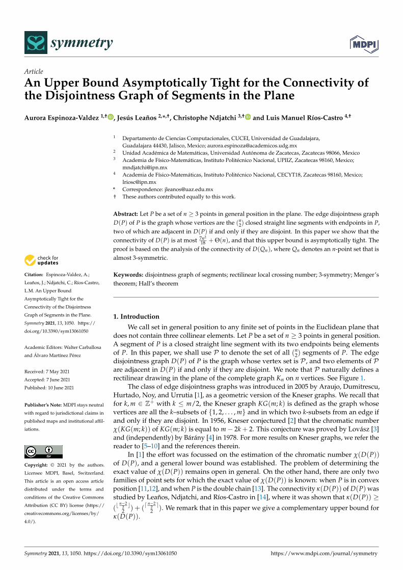
Figure 1. The point set P = {x1, x2, y1, y2, z1, z2} on the upper left is a set in general position. In theupper right we have P , which can be seen as the rectilinear drawing of K6 induced by P. As thelargest number of crossings on any segment of P is 1, then lcr(P) = 1. The graph on the bottom partis the edge disjointness graph D(P) corresponding to P.
Symmetry 2021, 13, 1050 3 of 13
Let H = (V(H), E(H)) be a (non-empty) simple connected graph. As usual, if u, v ∈V(H), then the distance between u and v in H will be denoted by dH(u, v), and we writeuv to mean that u and v are adjacent in H. We note that the uv notation is similar to thatused to denote the straight line segment xy defined by the points x, y ∈ P. However, noneof these notations should be a source of confusion, because the former objects are verticesof a graph, and the latter are points in the plane.
The neighborhood of v in H is the set {u ∈ V(H) : uv ∈ E(H)} and is denoted byNH(v). If S ⊆ V(H), then NH(S) := ∪v∈SNH(v). The degree degH(v) of v is the number|NH(v)|. The number δ(H) := min{degH(v) : v ∈ V(H)} is the minimum degree of H.A u − v path of H is a path of H having an endpoint in u and the other endpoint in v.Similarly, if U is a subgraph of H, then H \U is the subgraph of H that results by removingU from H.
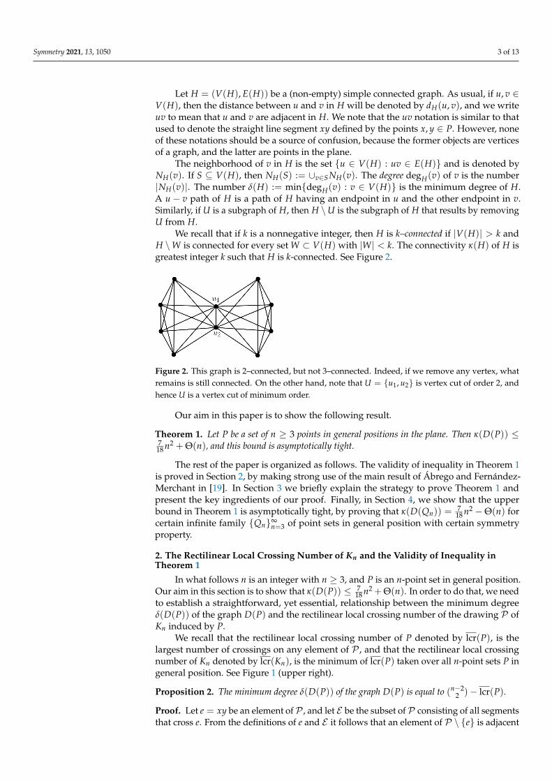
We recall that if k is a nonnegative integer, then H is k–connected if |V(H)| > k andH \W is connected for every set W ⊂ V(H) with |W| < k. The connectivity κ(H) of H isgreatest integer k such that H is k-connected. See Figure 2.
Figure 2. This graph is 2–connected, but not 3–connected. Indeed, if we remove any vertex, whatremains is still connected. On the other hand, note that U = {u1, u2} is vertex cut of order 2, andhence U is a vertex cut of minimum order.
Our aim in this paper is to show the following result.
Theorem 1. Let P be a set of n ≥ 3 points in general positions in the plane. Then κ(D(P)) ≤7
18 n2 + Θ(n), and this bound is asymptotically tight.
The rest of the paper is organized as follows. The validity of inequality in Theorem 1is proved in Section 2, by making strong use of the main result of Ábrego and Fernández-Merchant in [19]. In Section 3 we briefly explain the strategy to prove Theorem 1 andpresent the key ingredients of our proof. Finally, in Section 4, we show that the upperbound in Theorem 1 is asymptotically tight, by proving that κ(D(Qn)) =
718 n2 −Θ(n) for
certain infinite family {Qn}∞n=3 of point sets in general position with certain symmetry
property.
2. The Rectilinear Local Crossing Number of Kn and the Validity of Inequality inTheorem 1
In what follows n is an integer with n ≥ 3, and P is an n-point set in general position.Our aim in this section is to show that κ(D(P)) ≤ 7
18 n2 +Θ(n). In order to do that, we needto establish a straightforward, yet essential, relationship between the minimum degreeδ(D(P)) of the graph D(P) and the rectilinear local crossing number of the drawing P ofKn induced by P.
We recall that the rectilinear local crossing number of P denoted by lcr(P), is thelargest number of crossings on any element of P , and that the rectilinear local crossingnumber of Kn denoted by lcr(Kn), is the minimum of lcr(P) taken over all n-point sets P ingeneral position. See Figure 1 (upper right).
Proposition 2. The minimum degree δ(D(P)) of the graph D(P) is equal to (n−22 )− lcr(P).
Proof. Let e = xy be an element of P , and let E be the subset of P consisting of all segmentsthat cross e. From the definitions of e and E it follows that an element of P \ {e} is adjacent

Symmetry 2021, 13, 1050 4 of 13
to e in D(P) if and only if has both endpoints in P \ {x, y} and does not belong to E . Since|P| = n, then the degree of e in D(P) is exactly (n−2
2 )− |E|. The last fact and |E | ≤ lcr(P)imply δ(D(P)) ≥ (n−2
2 )− lcr(P). On the other hand, from the definition of lcr(P) we knowthat P contains a segment, say g, that is crossed by exactly lcr(P) elements of P \ {g}, andhence the degree of g in D(P) is (n−2
2 )− lcr(P), as required.
The following result was proved in [19] and is the key ingredient in the proof ofCorollary 4.
Theorem 3 (Theorem 1 [19]). If n is a positive integer, then
lcr(Kn) =
19 (n− 3)2 i f n ≡ 0 (mod 3),
19 (n− 1)(n− 4) i f n ≡ 1 (mod 3),
19 (n− 2)2 − b n−2
6 c i f n ≡ 2 (mod 3), n /∈ {8, 14}.
(1)
In addition, lcr(K8) = 4 and lcr(K14) = 15.
Corollary 4. Let P be an n-point set in general position, and let n ≥ 3. Then κ(D(P)) ≤7
18 n2 + Θ(n).
Proof. It is well-known that κ(D(P)) ≤ δ(D(P)). Thus, it suffices to show that δ(D(P)) ≤7
18 n2 + Θ(n). A trivial manipulation of Equation (1) allow us to see that lcr(Kn) =19 n2 −
Θ(n). On the other hand, from Proposition 2 and the fact that lcr(Kn) ≤ lcr(P), it followsthat δ(D(P)) ≤ (n−2
2 )− lcr(Kn) = (n−22 )−
(19 n2 −Θ(n)
)= 7
18 n2 + Θ(n), as required.
3. The Key Ingredients of the Proof of Theorem 1
Our strategy to prove that the upper bound in Theorem 1 is asymptotically tight isas follows. First, for any integer n with n ≥ 3, we define a certain n-point set in a generalposition, which we denote by Qn. The family {Qn}∞
n=3 was originally defined by Lara,Rubio-Montiel and Zaragoza in [20], where it was shown that lcr(Kn) =
19 n2 −Θ(n). More
recently, Ábrego and Fernández-Merchant [19] showed that lcr(Kn) = lcr(Qn) for anyn 6≡ 2 (mod 3). Then, we will give some notation and basic facts related to the connectivityof D(Qn), which will allow us to simplify the remaining part of the proof of Theorem 1.Finally, in Section 4.2, we will show that κ(D(Qn)) =
718 n2 −Θ(n).
We now recall a couple of classical results in graph theory which are fundamental inour proof.
Theorem 5 (Hall’s theorem). Let H be a bipartite graph with bipartition {A, B}, and let C be anelement of {A, B} of minimum cardinality. Then H contains a matching of size |C| if and only if|NH(S)| ≥ |S| for any S ⊆ C.
Theorem 6 (Menger’s theorem). A graph is k-connected if and only if it contains k pairwiseinternally disjoint paths between any two distinct vertices.
It is straightforward to check that the graph D(P) is connected for any n-point set Pin general position with n ≥ 5. In view of this, the following consequence of Menger’stheorem will be useful.
Corollary 7. Let H be a connected graph. Then H is k-connected if and only if H has k pairwiseinternally disjoint a− b paths, for any two vertices a and b of H such that dH(a, b) = 2.
Proof. The forward implication follows directly from Menger’s theorem. Conversely, letU be a vertex cut of H of minimum order. Let H1 and H2 be two distinct components ofH \U, and let u ∈ U. Since U is a minimum cut, then u has at least a neighbor vi in Hi, fori = 1, 2. Then dH(v1, v2) = 2. By hypothesis, H has k pairwise internally disjoint v1 − v2paths. Since each of these k paths intersects U, then we have that |U| ≥ k, as required.
Symmetry 2021, 13, 1050 5 of 13
Another ingredient that plays a central role in this work is the property of 3-symmetryof point sets in the plane, which is a recurrent concept in crossing number theory. A subsetX in R2 is called 3-symmetric if X contains a subset X1 such that X = X1 ∪ ρ(X1) ∪ ρ2(X1),where ρ is a 2π/3 clockwise rotation around a suitable point in the plane. The relationshipbetween the concept of 3-symmetry and several variants of crossing number have beeninvestigated by a number of authors [19–22]. If X is finite and |X| 6≡ 0 (mod 3), then wesay that X is almost 3-symmetric if X contains a subset X′ with at most two elements suchthat X \ X′ is 3-symmetric. As we shall see in the next section, the main part of the proof ofTheorem 1 is based on the estimation of the connectivity of D(Qn), where Qn is an almost3-symmetric set with n points.
4. The Upper Bound in Theorem 1 Is Asymptotically Tight
For the rest of the paper, n is an integer with n ≥ 3. We begin by introducing thefamily of point sets that we use in the proof of our main result, and some notation.
4.1. The Family {Qn}∞n=3 and Its Properties
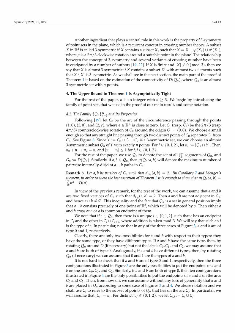
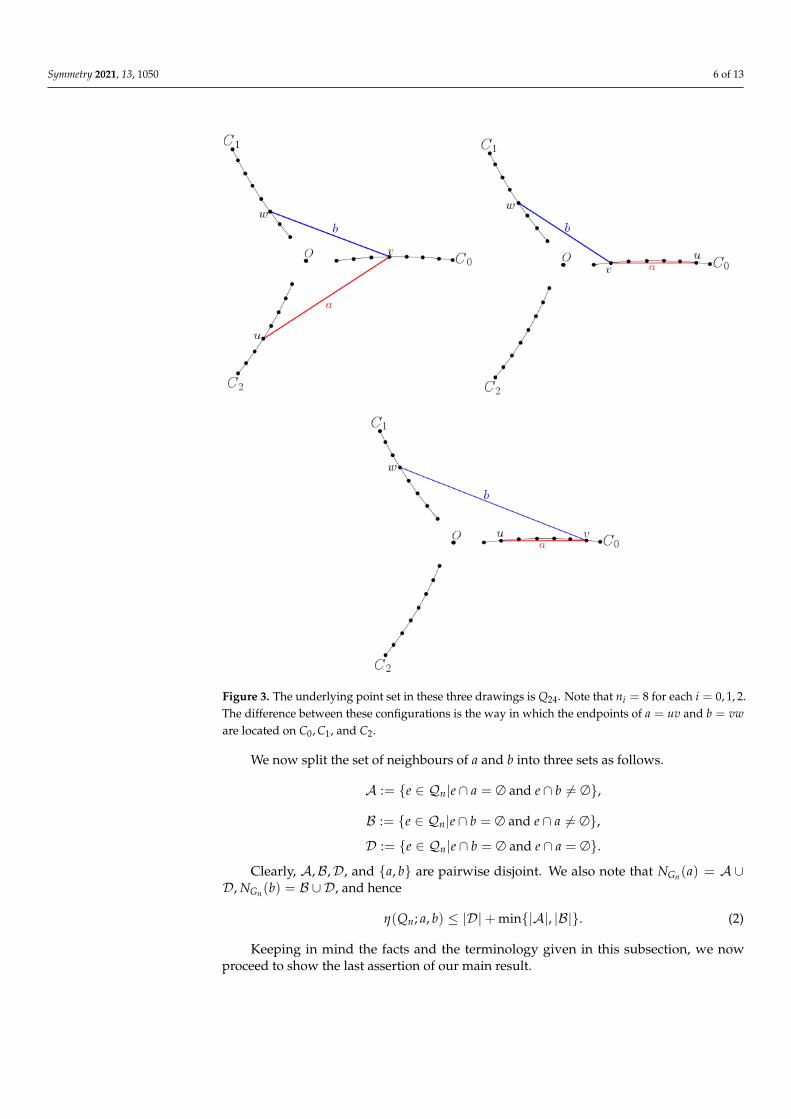
Following [19], let C0 be the arc of the circumference passing through the points(1, 0), (3, 0), and (2, ε), where ε ∈ R+ is close to zero. Let C1 (resp. C2) be the 2π/3 (resp.4π/3) counterclockwise rotation of C0 around the origin O := (0, 0). We choose ε smallenough so that any straight line passing through two distinct points of C0 separates C1 fromC2. See Figure 3. Since Y := C0 ∪ C1 ∪ C2 is a 3-symmetric set, we can choose an almost3-symmetric subset Qn of Y with exactly n points. For i ∈ {0, 1, 2}, let ni := |Qn ∩Y|. Then,n0 + n1 + n2 = n, and |ni − nj| ≤ 1 for i, j ∈ {0, 1, 2}.
For the rest of the paper, we use Qn to denote the set of all (n2) segments of Qn, and
Gn := D(Qn). Similarly, if a, b ∈ Qn, then η(Qn; a, b) will denote the maximum number ofpairwise internally-disjoint a− b paths in Gn.
Remark 8. Let a, b be vertices of Gn such that dGn(a, b) = 2. By Corollary 7 and Menger’stheorem, in order to show the last assertion of Theorem 1 it is enough to show that η(Qn; a, b) =7
18 n2 −Θ(n).
In view of the previous remark, for the rest of the work, we can assume that a and bare two fixed vertices of Gn such that dGn(a, b) = 2. Then a and b are not adjacent in Gn,and hence a ∩ b 6= ∅. This inequality and the fact that Qn is a set in general position implythat a ∩ b consists precisely of one point of R2, which will be denoted by o. Then either aand b cross at o or o is common endpoint of them.
We note that if e ∈ Qn, then there is a unique i ∈ {0, 1, 2} such that e has an endpointin Ci and the other in Ci ∪ Ci+2, where addition is taken mod 3. We will say that such an iis the type of e. In particular, note that in any of the three cases of Figure 3, a and b are oftype 0 and 1, respectively.
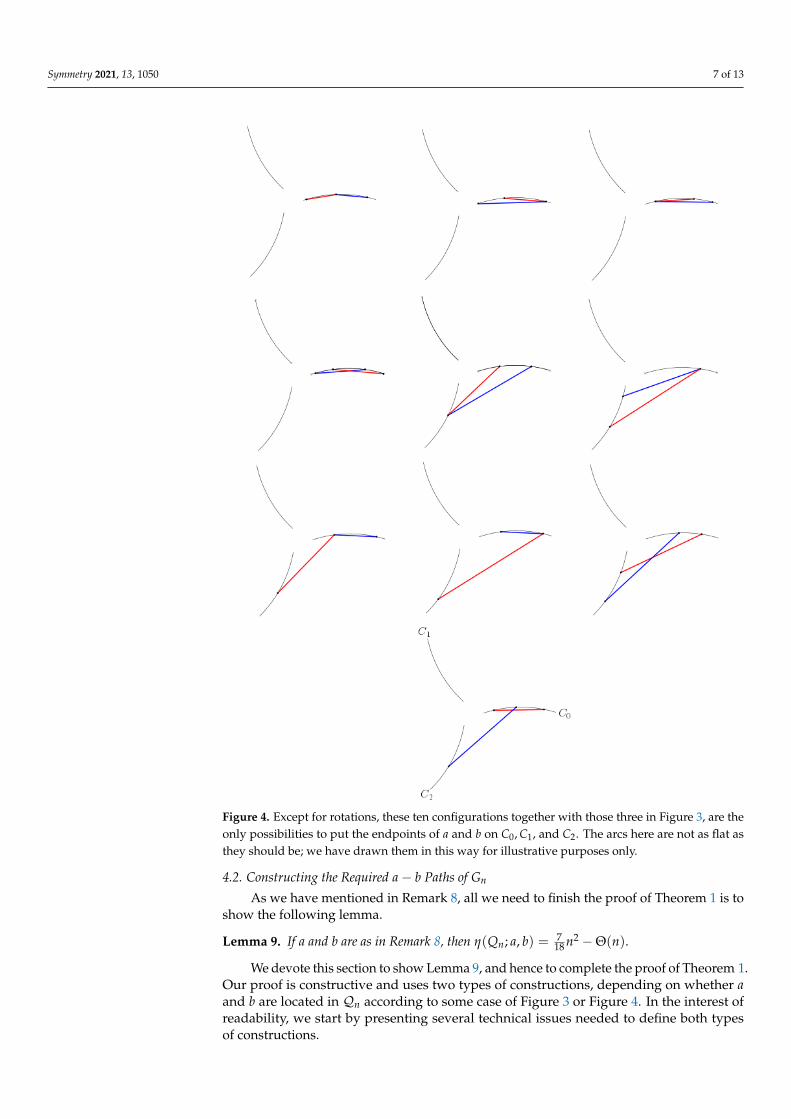
Clearly, there are only two possibilities for a and b with respect to their types: theyhave the same type, or they have different types. If a and b have the same type, then, byrotating Qn around O (if necessary) but not the labels C0, C1, and C2, we may assume thata and b are both of type 0. Analogously, if a and b have different types, then, by rotatingQn (if necessary) we can assume that 0 and 1 are the types of a and b.
It is not hard to check that if a and b are of type 0 and 1, respectively, then the threeconfigurations illustrated in Figure 3 are the only possibilities to put the endpoints of a andb on the arcs C0, C1, and C2. Similarly, if a and b are both of type 0, then ten configurationsillustrated in Figure 4 are the only possibilities to put the endpoints of a and b on the arcsC0 and C2. Then, from now on, we can assume without any loss of generality that a andb are placed in Qn according to some case of Figures 3 and 4. We abuse notation and weshall use Ci to refer to the subset of points of Qn that lies on the arc Ci. In particular, wewill assume that |Ci| = ni. For distinct i, j ∈ {0, 1, 2}, we let Ci,j := Ci ∪ Cj.
Symmetry 2021, 13, 1050 6 of 13
Figure 3. The underlying point set in these three drawings is Q24. Note that ni = 8 for each i = 0, 1, 2.The difference between these configurations is the way in which the endpoints of a = uv and b = vware located on C0, C1, and C2.
We now split the set of neighbours of a and b into three sets as follows.
A := {e ∈ Qn|e ∩ a = ∅ and e ∩ b 6= ∅},
B := {e ∈ Qn|e ∩ b = ∅ and e ∩ a 6= ∅},
D := {e ∈ Qn|e ∩ b = ∅ and e ∩ a = ∅}.
Clearly, A,B,D, and {a, b} are pairwise disjoint. We also note that NGn(a) = A ∪D, NGn(b) = B ∪D, and hence
η(Qn; a, b) ≤ |D|+ min{|A|, |B|}. (2)
Keeping in mind the facts and the terminology given in this subsection, we nowproceed to show the last assertion of our main result.
Symmetry 2021, 13, 1050 7 of 13
Figure 4. Except for rotations, these ten configurations together with those three in Figure 3, are theonly possibilities to put the endpoints of a and b on C0, C1, and C2. The arcs here are not as flat asthey should be; we have drawn them in this way for illustrative purposes only.
4.2. Constructing the Required a− b Paths of Gn
As we have mentioned in Remark 8, all we need to finish the proof of Theorem 1 is toshow the following lemma.
Lemma 9. If a and b are as in Remark 8, then η(Qn; a, b) = 718 n2 −Θ(n).
We devote this section to show Lemma 9, and hence to complete the proof of Theorem 1.Our proof is constructive and uses two types of constructions, depending on whether aand b are located in Qn according to some case of Figure 3 or Figure 4. In the interest ofreadability, we start by presenting several technical issues needed to define both typesof constructions.
Symmetry 2021, 13, 1050 8 of 13
Since the equality in Lemma 9 is asymptotic, in what remains of this section, weassume that n ≥ 15. Note that this assumption guarantees that each of C0, C1, and C2 hasat least one point that does not belong to a or b. This will be used in Section 4.2.2.
4.2.1. Suppose That a and b Have Distinct Types
Then, a and b are located in Qn according to some case of Figure 3, and so a =uv, b = vw, v ∈ C0, w ∈ C1, and u ∈ C0,2 \ {v}. Let H be the bipartite subgraph of Gn withbipartition {A,B} such that f ∈ A is adjacent to g ∈ B in H if and only if f and g areadjacent in Gn. Thus, H is an induced bipartite subgraph of Gn. If X and Y are nonemptysubsets of Qn, we will denote the set of all segments of Qn that have an endpoint in X andthe other in Y by X ∗Y.
A simple inspection of the several cases in which two elements of Qn can cross eachother yields the following assertion.
Observation 10. If f , g ∈ Qn cross each other, then f and g are of the same type.
A key fact that will allow us to construct the first class of paths is that H satisfies theHall’s condition. We formalize this idea as follows.
Proposition 11. Let C be an element of {A,B} of minimum cardinality. Then |NH(S)| ≥ |S|for any S ⊆ C.
Proof. We break the proof into two cases, depending on whether |A| ≤ |B| or |A| > |B|.We remark that Observation 10 is often used in this proof without explicit mention.
(A) Suppose that |A| ≤ |B|, and let S ⊆ A. We can assume that S 6= ∅ and thatB \ NH(S) 6= ∅, as otherwise we are done. Let e∗ be a fixed segment of B \ NH(S), andassume that e∗ = pq.
The next facts follow easily from the choice of e∗ and S . (F1) e∗ intersects each elementof S ∪ {a}, (F2) b intersects each element of S , and (F3) each element of S has at least oneendpoint in C1.
(A1) Suppose that p ∈ C0 and q ∈ C2. Then (F1) and (F3) imply that S is a subset ofA′ := X ∪{qw}, whereX denotes the set of all segments that intersect b and are in {p} ∗C1.Note that if S = {qw}, then {u} ∗ (C0 \ {u, v}) ⊆ NH(S), and so |NH(S)| ≥ n0 − 2 ≥1 = |S|. Thus, we may assume that X 6= ∅. This implies that if qw ∈ S (respectively,qw /∈ S), then B′ := {u} ∗ (C0,2 \ {q, u, v}) (respectively, B′ := {u} ∗ (C0,2 \ {p, u, v})) is asubset of NH(S). Since |A′| ≤ n1 + 1, |B′| ≥ n0 + n2 − 3 and n0 + n2 ≥ n1 + 4, we have|NH(S)| ≥ |S|.
(A2) Suppose that p, q ∈ C0. Then (F1) and (F3) imply that S is a subset of the set A′,which consists of all segments that intersect b and are in {p, q} ∗C1. Then, |S| ≤ |A′| ≤ 2n1.Let e ∈ S , and assume without loss of generality that p ∈ e. Since e∩ a = ∅, then p /∈ {u, v}and B′ := {u} ∗ (C0,2 \ {u, v, p}) is a subset of NH(e). Then, |NH(S)| ≥ |B′| = n0 + n2− 3,and we can assume that |A′| > n0 + n2 − 3, as otherwise we are done. This implies thatthere exists g ∈ S with q ∈ g.
Since u ∈ C2 implies |A′| ≤ n1 + 1 < n0 + n2 − 3, we can assume that u ∈ C0. Let I0be the set of points of C0 that are between u and v. From (F1) we know that at most oneof p or q is in I0. If z ∈ {p, q} is a point of I0, then B′ ∪ ({z} ∗ C2) is a subset of NH({e, g}).Then |NH(S)| ≥ (n0 + n2 − 3) + n2 ≥ 2n1 ≥ |S|, as required. Then, neither p nor q isin I0. Since e∗ ∩ a 6= ∅, we must have u = q. This implies that S ⊆ {p} ∗ C1, and so|NH(S)| ≥ n0 + n2 − 3 ≥ n1 ≥ |S|.
(A3) Suppose that p, q ∈ C2. Since e∗ is of type 2 and e∗ ∩ a 6= ∅, then u must be acommon endpoint of e∗ and a, by Observation 10. Without loss of generality, suppose thatp = u.
From (F1) and (F3) we know that S is a subset of {w} ∗ (Y ∪ {q}), where Y denotes theset of all points of C2 that lie between u and q. Note that if u and q are consecutive points ofC2, then Y = ∅. Let e be the segment of S whose endpoint q′ ∈ Y ∪ {q} is closest to q. LetY′ be the set of all points of C2 that lie between u and q′. Then |Y′|+ 1 ≥ |S|, and B′ :=

Symmetry 2021, 13, 1050 9 of 13
{u} ∗ (Y′ ∪ C0 \ {v}) is a subset of NH(e). Since |S| ≤ |Y′|+ 1 and |B′| = (n0 − 1) + |Y′|,then n0 ≥ 5 implies |NH(S)| ≥ |S|.
(A4) Suppose that e∗ has an endpoint in C1. We assume without loss of generality thatp ∈ C1. Clearly, p 6= w. Since e∗ ∩ a 6= ∅, then q = u, and so q ∈ C0,2 \ {v}.
(A4.1) Suppose that q ∈ C0 \ {v}. Then e∗, b ∈ C1 ∗ {u, v}, and e∗ ∩ b = ∅. Sinceu, v ∈ C0, then {w} ∗ C2 ⊆ A \ S due to (F1). Let A′ := A \ ({w} ∗ C2), and let B′ be theset that results by removing any segment of {u} ∗ (C1 \ {p}) from B. Then, |B′| ≥ |A′|because |B| ≥ |A|. We note that (F1) implies S ⊆ A′. If S contains a segment e with bothendpoints in C1, then (F1) implies B′ ⊆ NH(e), and hence |NH(S)| ≥ |B′| ≥ |A′| ≥ |S|, asrequired. Thus, we may assume that S ∩ (C1 ∗ C1) = ∅, and so S ⊆ C0 ∗ C1.
Let I0 be the set of points of C0 that are between u and v (if u and v are contiguous,I0 = ∅), and let J0 := C0 \ (I0 ∪ {v}). By (F1) and (F2) we know that each segment of Sintersects both e∗ and b. Since b and e∗ are disjoint, no segment of S can have an endpointin I0 ∪ {v}, and, on the other hand, each segment of B′ must have at least one endpointin I0 ∪ {u}. Note that if J0 has at least two points being incident with segments of S , theneach segment of B′ is disjoint from at least one of these points of J0, and hence B′ ⊆ NH(S),as required.
Thus, we can assume that all segments of S are incident with one point of J0, say z.Then, S ⊆ {z} ∗ (C1 \ {p}) or S ⊆ {z} ∗ (C1 \ {w}), and so |S| ≤ n1 − 1 ≤ n2. On theother hand, note that {u} ∗ C2 ⊆ NH(S), and so |NH(S)| ≥ n2, as required.
(A4.2) Suppose now that q ∈ C2. Then (F1), (F2), and (F3) imply that each segmentof S must be incident with at least one of p or w. Then, S is the disjoint union Sp andSw, where Sp (respectively, Sw) denotes the subset of S contained in {p} ∗ (C0,1 \ {p, v})(respectively, {w} ∗ (C2 \ {u})). Then, |S| = |Sp|+ |Sw| ≤ (n0 + n1 − 2) + (n2 − 1).
Let B1u := {u} ∗ (C1 \ {p, w}) and B0,2
u := {u} ∗ (C0,2 \ {u, v}). Clearly, B1u and B0,2
u
are disjoint sets. Moreover, by (A1) and (A3), we may assume that B0,2u ⊂ NH(S).
Suppose first that Sp has no segments in {p} ∗ (C0 \ {v}). Then Sp ⊆ {p} ∗ (C1 \ {p}),and so |S| = |Sp|+ |Sw| ≤ (n1− 1)+ (n2− 1). We may assume that n0 + n2− 2 = |B0,2
u | ≤|NH(S)| < |Sp|+ |Sw| ≤ n1 + n2 − 2, as otherwise we are done. Since n0 ≥ n1 − 1, thenwe must have that n0 = n1 − 1,Sp = {p} ∗ (C1 \ {p}), and Sw = {w} ∗ (C2 \ {u}). FromSp = {p} ∗ (C1 \ {p}) it follows that pw ∈ S , and hence B1
u ⊂ NH(pw) ⊂ NH(S). SinceB1
u and B0,2u are pairwise disjoint, |NH(S)| ≥ (n0 + n2− 2) + (n1− 2) > n1 + n2− 2 ≥ |S|,
as required.Suppose now that Sp has a segment e in {p} ∗ (C0 \ {v}). Then B1
u ⊂ NH(e) ⊂NH(S), and hence |NH(S)| ≥ |B0,2
u | + |B1u| = (n0 + n2 − 2) + (n1 − 2). Thus, we may
assume that |Sp| = n0 + n1 − 2 and |Sw| = n2 − 1, as otherwise we are done. Then,Sp = {p} ∗ (C0,1 \ {p, v}) and Sw = {w} ∗ (C2 \ {u}).
From Sp = {p} ∗ (C0,1 \ {p, v}) and (F2) it is not hard to see that vp must be thesegment of C0 ∗ C1 with either the smallest or the largest length. Let B′ := (C0 \ {v}) ∗(C2 \ {u}). If vp is the segment of C0 ∗ C1 with the smallest (respectively, largest) length,then Sw = {w} ∗ (C2 \ {u}) and (F1) imply that pu must have the largest (respectively,smallest) length among all segments in {p} ∗ C2, and hence B′ ⊂ NH(S). Since B1
u, B0,2u ,
and B′ are pairwise disjoint and |B′| ≥ (n0 − 1)(n2 − 1) ≥ 4, then |NH(S)| ≥ (n0 + n2 −2) + (n1 − 2) + 4 > |S|, as required.
(B) Suppose that |B| < |A|, and let S ⊆ B. We can assume that S 6= ∅ and thatA\NH(S) 6= ∅, as otherwise we are done. Let d : R2 → R≥0 denote the ordinary euclideandistance in R2. For i ∈ {0, 1, 2} and x ∈ Ci, we let C>x
i := {y | y ∈ Ci and d(O, y) >d(O, x)}. The set C<x
i is defined analogously. It is not hard to see that A ⊆ F , where
F := ({w} ∗ (Qn \ {u, v, w})) ∪ (C<v0 ∗ C>w
1 ) ∪ (C>v0 ∗ C<w
1 ) ∪ (C<w1 ∗ C>w
1 ).
Note that Fw := {w} ∗ (Qn \ {u, v, w}) is a subset of A. Since no segment of Bintersects every segment of Fw, then at least one segment of Fw is in NH(S), and so|NH(S)| ≥ 1. Thus |S| ≥ 2, as otherwise we are done.
Symmetry 2021, 13, 1050 10 of 13
(B1) Suppose that S has two distinct segments of type 0, say e1 and e2, so that e1 ∩e2 ∩ C0 = ∅. Then A ⊆ NH({e1, e2}) ⊆ NH(S), unless e1 ∩ e2 = y ∈ C2. Since the formercase contradicts A \ NH(S) 6= ∅, we assume that e1 ∩ e2 = y ∈ C2. Then A \ {yw} ⊆NH({e1, e2}), and hence |NH(S)| ≥ |NH({e1, e2})| ≥ |A| − 1 ≥ |B| ≥ |S|, as required.
(B2) Suppose now that each segment of S is incident with exactly one point x ∈ C0.Clearly, x 6= v. If x 6= u, then S ⊆ {x} ∗ (C0,2 \ {x, v}), and hence |S| ≤ n0 + n2 − 2. Since|S| ≥ 2, then C0,2 \ {x, v} has at least two points, say z1 and z2, such that xz1, xz2 ∈ S .We note that Fw \ {wx} ⊆ NH({xz1, xz2}) ⊆ NH(S), and so |NH(S)| ≥ |Fw| − 1 ≥n0 + n1 + n2 − 4. Since n1 ≥ 3, then |NH(S)| ≥ n0 + n2 − 1 ≥ |S|.
Suppose now that u = x. Then S ⊆ {u} ∗ (Qn \ {u, v, w}), and so |S| ≤ n0 + n1 +n2 − 3. If S has at least one segment in {u} ∗ C2, then |S| ≥ 2 implies that Fw ⊆ NH(S),and so |NH(S)| ≥ |Fw| ≥ n0 + n1 + n2 − 3 ≥ |S|. Then, we may assume that S has nosegments in {u} ∗ C2, and hence {w} ∗ C2 ⊆ NH(S).
Let W1 be the subset of all points in C1 that are incident with a segment of S . ThenS ⊆ {u} ∗ (W1 ∪ C0 \ {u, v}), and so |S| ≤ |W1|+ n0 − 2. If W1 = ∅, then |S| ≤ n0 − 2 ≤n2 = |{w} ∗ C2| ≤ |NH(S)|, as required. Then we can assume that W1 6= ∅. Let w′
be the point in W1 that is farthest from w. Since any segment in {w} ∗ (W1 \ {w′}) isdisjoint from uw′, then F ′w := {w} ∗ (C2 ∪ (W1 \ {w′})) is a subset of NH(S), and hence|NH(S)| ≥ |F ′w| ≥ |W1| − 1 + n2 ≥ |W1|+ n0 − 2 ≥ |S|.
(B3) Suppose that u ∈ C2. Let S ′ be the set of all segments of S that are not incidentwith u. Suppose first that S ′ = ∅. Then (B1) implies that S has at most one segment in{u} ∗C0. If there exists x ∈ C0 such that ux ∈ S , then |S| ≥ 2 implies thatA ⊆ NH(S), andhence |NH(S)| ≥ |A| > |B| ≥ |S|. Thus, we may assume that S ⊆ {u} ∗ (C1,2 \ {u, w}).For k = 1, 2, let Wk be the subset of all points in Ck \ {u, w} that are incident with asegment of S . Then S = {u} ∗ (W1 ∪W2), and so |S| = |W1| + |W2|. If Wk 6= ∅, thenwe use wk to denote the point in Wk that is closest to w if k = 1 (resp. u if k = 2).Since any segment in {w} ∗ (Wk \ {wk}) is disjoint from at least one of uw1 or uw2, thenF ′w := {w} ∗ ((C0 ∪W1 ∪W2) \ {v, w1, w2}) is a subset of NH(S), and hence |NH(S)| ≥|F ′w| ≥ n0 + |W1|+ |W2| − 3 ≥ |W1|+ |W2| ≥ |S|.
Suppose now that S ′ 6= ∅. Then each segment of S ′ crosses a, and has at least oneendpoint in C0 \ {v}. From (B2) it follows that there is x ∈ C0 \ {v} such that S ′ ⊆ {x} ∗C2.This fact and (B2) imply the existence of uy ∈ S with y ∈ C1,2 \ {u, w}. Note that if|S ′| > 1, then A \ {xy} ⊆ NH(S ′ ∪ {uy}) ⊆ NH(S). On the other hand, if S ′ = {xz}for some z ∈ C2 \ {u}, then A \ {wz} ⊆ NH({xz, uy}) ⊆ NH(S). In any case, we have|NH(S)| ≥ |A| − 1 ≥ |B| ≥ |S|.
(B4) Suppose that u ∈ C0. Let Su be the set of all segments of S in {u} ∗ (C1 \ {w}),and let S ′ = S \ Su. Then, any element in S ′ is a segment of type 0. We may assumethat Su 6= ∅, as otherwise we are in (B1) or (B2) due to |S| ≥ 2. Similarly, if S ′ = ∅,then |S| = |Su| ≤ n1 − 1. From Su 6= ∅ we have that {w} ∗ C2 ⊆ NH(S), and so|NH(S)| ≥ n2 ≥ n1 − 1 ≥ |S|. Thus, we also assume that S ′ 6= ∅.
From (B1) and S ′ 6= ∅ we know that there exists a point x ∈ C0 \ {v} that is incidentwith any segment of S ′. Since {w} ∗ C2 ⊆ NH(Su) and {w} ∗ (C0 ∪ C1 \ {u, v, x, w}) ⊆NH(S ′), then |NH(S)| ≥ n0 + n1 + n2 − 4. Seeking a contradiction, suppose that |S| ≥n0 + n1 + n2− 3. Since |Su| ≤ n1− 1, then |S ′| ≥ n0 + n2− 2. From S ′ ⊆ {x} ∗C0,2 \ {x, v}and n0 ≥ 3 it follows that S ′ has a segment e = xy with y ∈ C0 \ {x, v}. Since e togetherwith any other e′ ∈ S ′ \ {e} satisfy the conditions of (B1), then we must have that S ′ = {e},contradicting |S ′| ≥ n0 + n2 − 2.
4.2.2. Suppose That a and b Have The Same Type
Then, a and b are located inQn according to some case of Figure 4. For i = 0, 1, 2 let Eibe the set of points in Ci that are endpoints of at least one of a and b, and let C′i := Ci \ Ei.Then, 3 ≤ |E0|+ |E1|+ |E2| ≤ 4. From a simple inspection of the ten cases in Figure 4

Symmetry 2021, 13, 1050 11 of 13
we can see that |E0| ∈ {1, 2, 3, 4}, |E1| = 0, and |E2| ∈ {0, 1, 2}. Thus, for i = 0, 1, 2 thefollowing holds:
bn/3c+ 1 ≥ |Ci| ≥ |C′i | ≥ bn/3c − 4 ≥ 1. (3)
Let G′n be the subgraph of Gn induced by C0,2, i.e., G′n := D(C0,2). Similarly, let
D1 := (C1 ∗ C1) ∪ (C1 ∗ C′0) ∪ (C1 ∗ C′2).
It is easy to check that D1 and G′n satisfy the following properties: (i) the three setsforming D1 are pairwise disjoint, (ii) no segment of D1 belongs to G′n, (iii) D1 ⊆ D, and (iv)a and b are vertices of G′n.
By applying the main result of [14] to G′n we have that the connectivity of G′n is at least
κ′n :=(bm−2
2 c2
)+
(dm−2
2 e2
), (4)
where m = |C0,2|.
We are finally ready to prove Lemma 9.
Proof of Lemma 9. We analyze two cases separately, depending on whether a and b arelocated in Qn according to some case of Figure 3 or Figure 4.
Case 1. Suppose that a and b are located inQn according to some case of Figure 3, andlet H ⊆ Gn be as in Section 4.2.1. From Proposition 11 and Hall’s theorem it follows thatH has a matching M of size m1 := min{|A|, |B|}. Suppose that M = {akbk | ak ∈ A, bk ∈B, and k = 1, 2, . . . , m1}. Then
L :={
aakbkb | akbk ∈ M}
,
is a collection a − b paths of Gn of length 3. Furthermore, the paths in L are pairwiseinternally disjoint, because M is a matching of H. On the other hand, note that
L′ :={
adb | d ∈ D}
,
is also a collection of pairwise internally disjoint a − b paths of Gn of length 2. SinceD ∩ (A∪B) = ∅, then the paths in L∪L′ are pairwise internally disjoint. The existence ofsuch m1 + |D| paths, and (2) imply
η(Qn; a, b) = |D|+ m1 = |D|+ min{|A|, |B|} = min{degGn(a), degGn
(b)}. (5)
Combining Proposition 2 and Theorem 3 we obtain that δ(Gn) =7
18 n2 + Θ(n). Sincemin{degGn
(a), degGn(b)} ≥ δ(Gn), then (2) and (5) imply η(Qn; a, b) = 7
18 n2 + Θ(n) =7
18 n2 −Θ(n), as required.Case 2. Suppose now that a and b are located inQn according to some case of Figure 4,
and let G′n, C′i ,D1, κ′n, m, and Properties (i)–(iv) as in Section 4.2.2.Since 2b n
3 c ≤ m ≤ 2b n3 c+ 2, a straightforward manipulation on (4) gives that k′n =
218 n2 −Θ(n). This last equality, (iv), and Menger’s theorem imply that G′n has collection Tof at least 2
18 n2 −Θ(n) pairwise internally disjoint a− b paths. On the other hand, from(iii) it follows that
T′ :={
adb | d ∈ D1}
,
is a collection of |D1| pairwise internally disjoint a− b paths of Gn of length 2. Moreover,by (ii) we have that T∪T′ is also a collection of pairwise internally disjoint a− b paths ofGn. From (3), (i), and the definition of T′, it is not hard to see that
|T′| = |D1| =(|C1|
2
)+ |C1||C′0|+ |C1||C′2| ≥
518
n2 −Θ(n).

Symmetry 2021, 13, 1050 12 of 13
Thus, η(Qn; a, b) ≥ |T ∪ T′| ≥ 718 n2 − Θ(n). This last and (2) imply η(Qn; a, b) =
718 n2 −Θ(n), as required. �
5. Concluding Remarks
Let P be a set of n ≥ 3 points in general position in the plane. We have observed thatthe minimum degree δ(D(P)) of the disjointness graph of segments defined by P can beexpressed in terms of n and the rectilinear local crossing number of the rectilinear drawingP of Kn induced by P. From this observation and the exact value of lcr(Kn) providedby Theorem 1 in [19], it is easy to see that (n
2)− lcr(Kn) is an upper bound for δ(D(P)),which is tight for each n. Since the connectivity κ(H) of a graph H is upper bounded by itsminimum degree δ(H), then (n
2)− lcr(Kn) is also a general upper bound for κ(D(P)).On the other hand, the main goal in this work is to estimate the connectivity of D(Qn),
where {Qn}∞n=3 is one of the families of point sets best understood from the point of view
of rectilinear crossing number. In particular, it is known that Qn is almost 3-symmetricand that lcr(Kn) = lcr(Qn) for each n 6≡ 2 (mod 3). The basic idea behind our approachis to show that δ(D(Qn)) − κ(D(Qn)) cannot be too large. In fact, we strongly believethat δ(D(Qn)) = κ(D(Qn)) holds, and that this equality can be verified by analogousarguments to those used in Section 4.2.1. We finally remark that Theorem 1 is an asymptoticsolution for an open question posed in [14].
Author Contributions: The authors contributed equally to this work. All authors have read andagreed to the published version of the manuscript.
Funding: This research received no external funding.
Institutional Review Board Statement: Not applicable.
Informed Consent Statement: Not applicable.
Data Availability Statement: Not applicable.
Acknowledgments: We thank two anonymous referees for careful reading and improvements to thepresentation.
Conflicts of Interest: The authors declare no conflict of interest.
References1. Araujo, G.; Dumitrescu, A.; Hurtado, F.; Noy, M.; Urrutia, J. On the chromatic number of some geometric type Kneser graphs.
Comput. Geom. 2005, 32, 59–69. [CrossRef]2. Kneser, M., Aufgabe 360 , Jahresbericht der Deutschen Mathematiker-Vereinigung. Abteilung 1955, 58, 27.3. Lovász, L. Kneser’s conjecture, chromatic number, and homotopy. J. Combin. Theory Ser. A 1978, 25, 319–324. [CrossRef]4. Bárány, I. A short proof of Kneser’s conjecture. J. Combin. Theory Ser. A 1978, 25, 325–326. [CrossRef]5. Chen, Y.-C. Kneser graphs are Hamiltonian for n ≥ 3k. J. Combin. Theory Ser. B 2000, 80, 69–79. [CrossRef]6. Ekinci, G.B.; Gauci, J.B. The super-connectivity of Kneser graphs. Discuss. Math. Graph Theory 2019, 39, 5–11. [CrossRef]7. Albertson, M.O.; Boutin, D.L. Using determining sets to distinguish Kneser graphs. Electron. J. Combin. 2007, 14, 20. [CrossRef]8. Matousek, J. Using the Borsuk-Ulam theorem. In Lectures on Topological Methods in Combinatorics and Geometry; Anders, B., Günter,
M.Z., Eds.; Springer: Berlin, Germany, 2003; ISBN 3-540-00362-2.9. Valencia-Pabon, M.; Vera, J.-C. On the diameter of Kneser graphs. Discret. Math. 2005, 305, 383–385. [CrossRef]10. Reinfeld, P. Chromatic Polynomials and the Spectrum of the Kneser Graph. Tech. rep., London School of Economics. LSE-
CDAM-2000-02. 2000. Available online: http://citeseerx.ist.psu.edu/viewdoc/summary?doi=10.1.1.27.4627 (accessed on 7June 2021).
11. Jonsson, J. The Exact Chromatic Number of the Convex Segment Disjointness Graph. 2011. Available online: https://people.kth.se/~jakobj/doc/preprints/chrom.pdf (accessed on 7 June 2021).
12. Fabila-Monroy, R.; Wood, D.R. The chromatic number of the convex segment disjointness graph. In Computational Geometry,Volume 7579 of Lecture Notes in Computer Science; Springer: Cham, Switzerland, 2011; pp. 79–84.
13. Fabila-Monroy, R.; Hidalgo-Toscano, C.; Leaños, J.; Lomelí-Haro, M. The Chromatic Number of the Disjointness Graph of theDouble Chain. Discret. Math. Theor. Comput. Sci. 2020, 22, 11.
14. Leaños, J.; Ndjatchi, C.; Ríos-Castro, L.R. On the connectivity of the disjointness graph of segments of point sets in generalposition in the plane. arXiv 2007, arXiv:2007.15127v1.

Symmetry 2021, 13, 1050 13 of 13
15. Aichholzer, O.; Kyncl, J.; Scheucher, M.; Vogtenhuber, B. On 4–Crossing-Families in Point Sets and an Asymptotic Upper Bound.In Proceedings of the 37th European Workshop on Computational Geometry (EuroCG 2021), Saint Petersburg, Russia, 7–9 April2021; pp. 1–8.
16. Pach, J.; Tardos, G.; Tóth, G. Disjointness graphs of segments. In 33th International Symposium on Computational Geometry (SoCG2017) of Leibniz International Proceedings in Informatics (LIPIcs); Katz 59; Boris, A., Matthew, J., Eds.; Leibniz-Zentrum für Informatik:Wadern, Germany, 2017; Volume 77, pp. 1–15.
17. Pach, J.; Tomon, I. On the Chromatic Number of Disjointness Graphs of Curves. In 35th International Symposium on ComputationalGeometry (SoCG 2019); Schloss Dagstuhl-Leibniz-Zentrum fuer Informatik: Wadern, Germany, 2019.
18. Pach, J. Geometric Graph Theory, Surveys in Combinatorics, BOOK_CHAP. 1999; pp. 167–200. Available online:https://www.cambridge.org/core/books/surveys-in-combinatorics-1999/geometric-graph-theory/E57E1273C7FAA8FD47B1B28F0E539C90 (accessed on 7 June 2021).
19. Ábrego, B.M.; Fernández-Merchant, S. The rectilinear local crossing number of Kn. J. Combinat. Ser. A 2017, 151, 131–145.[CrossRef]
20. Lara, D.; Rubio-Montiel, C.; Zaragoza, F. Grundy and pseudo–Grundy indices for complete graphs. In Proceedings of theAbstracts of the XVI Spanish Meeting on Computational Geometry, Barcelona, Spain, 1–3 July 2015.
21. Ábrego, B.M.; Cetina, M.; Fernández-Merchant, S.; Leaños, J.; Salazar, G. 3-symmetric and 3–decomposable geometric drawingsof Kn. Discret. Appl. Math. 2010, 158, 1240–1258. [CrossRef]
22. Ábrego, B.M.; Cetina, M.; Fernández-Merchant, S.; Leaños, J.; Salazar, G. On≤k-Edges, Crossings, and Halving Lines of GeometricDrawings of Kn. Discret. Comput. Geom. 2012, 48, 192–215. [CrossRef]