An updated kernel-based Turing model for 1

studying the mechanisms of biological 2

pattern formation 3

4

5

Shigeru Kondo 6

7

Graduate School of Frontier Biosciences 8

Osaka University 9

1-3 Yamadaoka, Suita, Osaka, 565-0871, Japan 10

Phone +81-6-9879-7975 11

Fax +81-6-9879-7977 12

13

14

15

Abstract 16

17

The reaction-diffusion model presented by Alan Turing has recently been supported by experimental 18

data and accepted by most biologists. However, scientists have recognized shortcomings when the 19

model is used as the working hypothesis in biological experiments, particularly in studies in which 20

the underlying molecular network is not fully understood. To address some such problems, this 21

report proposes a new version of the Turing model. 22

This improved model is not represented by partial differential equations, but rather by the shape of 23

an activation-inhibition kernel. Therefore, it is named the kernel-based Turing model (KT model). 24

Simulation of the KT model with kernels of various shapes showed that it can generate all standard 25

variations of the stable 2D patterns (spot, stripes and network), as well as some complex patterns that 26

are difficult to generate with conventional mathematical models. The KT model can be used even 27

when the detailed mechanism is poorly known, as the interaction kernel can often be detected by a 28

simple experiment and the KT model simulation can be performed based on that experimental data. 29

These properties of the KT model complement the shortcomings of conventional models and will 30

contribute to the understanding of biological pattern formation. 31

32

Key words 33

Turing pattern, reaction-diffusion model, pattern formation, kernel, pigmentation pattern, zebrafish, 34

LALI model 35

36

37

Competing interest 38

I have no competing interest. 39

40

Background 41

42

The reaction-diffusion (RD) model presented by Alan Turing in 1952[1] is a theoretical mechanism 43

to explain how spatial patterns form autonomously in an organism. In his classic paper, Turing 44

examined the behaviour of a system in which two diffusible substances interact with each other, and 45

found that such a system is able to generate a spatially periodic pattern even from a random or 46

almost uniform initial condition. Turing hypothesized that the resulting wavelike patterns are the 47

chemical basis of morphogenesis. 48

49

Although Turing’s theory was not sufficiently supported by experimental evidence for many years[2], 50

it has since been adapted by many mathematical researchers who showed that a wide variety of 51

patterns seen in organisms can be reproduced by the RD model[3, 4]. Meinhardt and Gierer stated 52

that the condition of “local activation with long-range inhibition (LALI)” is sufficient for stable 53

pattern formation [5]. This indication was quite important because it suggested that other effects on 54

cells (for example, cell migration, physical stress, and neural signals) could replace the effect of 55

diffusion in the original Turing model. Many different models have been presented to account for 56

situations in which diffusion might not occur [6-9]. However, in all cases, LALI is the anticipated set 57

of conditions sufficient to form the periodic pattern, and the pattern-formation ability is similar. 58

Therefore, these models are also called LALI models[10]. 59

60

The importance of the Turing model is obvious[11], in that it provided an answer to the fundamental 61

question of morphogenesis: “how is spatial information generated in organisms?” However, most 62

experimental researchers were sceptical until the mid-90s because little convincing evidence had 63

been presented[2]. In 1991, two groups of physicists succeeded in generating the Turing patterns in 64

their artificial systems, which showed for the first time that the Turing wave is not a fantasy but a 65

reality in science[12, 13]. Four years later, it was reported that the stripes of colour on the skin of 66

some tropical fishes are dynamically rearranged during their growth in accordance with Turing 67

model predictions[14, 15]. Soon after, convincing experimental evidence claiming the involvement 68

of a Turing mechanism in development has been reported[16] [17-19], and in some cases, the 69

candidate diffusible molecules were suggested. Currently, the Turing model has been accepted as one 70

of the fundamental mechanisms that govern morphogenesis[20, 21]. 71

72

On the other hand, experimental researchers have pointed out problem that occur when the LALI 73

models are used as the working hypothesis. For instance, LALI models can exhibit similar properties 74

of pattern formation despite being based on different cellular and molecular functions[10]. Therefore, 75

the simulation of a model rarely helps to identify the detailed molecular mechanism [22]. Even when 76

a pattern-forming phenomenon is successfully reproduced by the simulation of an RD system, it 77

does not guarantee the involvement of diffusion. This problem is quite serious because, in most 78

experimental uses, the key molecular event that governs the phenomenon is unknown when the 79

experimental project begins. 80

81

It has also become clear that the pre-existing LALI models cannot represent some real biological 82

phenomena. In the formation of skin pigmentation patterns in zebrafish, the key factors are cell 83

migration and apoptosis induced by direct physical interaction of cell projections[23-25]. This is 84

not the only case in which the key signals for pattern formation are transferred not by diffusion but 85

by fine cell projections such as filopodia[26-28], which may be essentially different than signalling 86

by diffusion. In diffusion, the concentration of the substance is highest at the position of the source 87

cell and rapidly decreases depending on the distance from the source. Therefore, it is difficult to use 88

diffusion to model the condition in which the functional level of the signal has a sharp peak at a 89

location distant from the source (Figure 1). As each LALI model is restricted by its assumed 90

signalling mechanism, it is difficult to adapt a model to an arbitrary stimulation-distance profile of a 91

real system. In this report, I present a new version of the Turing model that complements the 92

shortcomings of conventional models. 93

94

95

Model concept and description 96

97

In the modelling of systems that include non-local interactions, the integral function is useful. For 98

example, in the case of a neuronal system, the change of firing rate n at position x is represented by 99

[4](2nd

ed. Section 11) 100

Here, w(x-x’) is the kernel function, which quantifies the effect of the neighbouring n(x’,t) on n(x,t) 101

depending on the spatial distance. In this model system, the shape of the kernel determines how the 102

system behaves. The Fourier transform (FT) of the kernel produces the dispersion relation, which 103

shows the unstable (amplifying) wavelength. Importantly, this kernel method can be used to model 104

the effect of long-range diffusion that results from a local interaction. Murray proposed that “this 105

approach provides a useful unifying concept” [4]. The LALI condition can be considered the kernel 106

shape that makes stable waves. Thus, one simple method to generalize the conventional Turing or 107

LALI models would be to directly input an arbitrary kernel shape not based on the assumption of 108

any concrete molecular or cellular events. Such a model can be called a kernel-based Turing model 109

(KT model). 110

111

As the KT model is not based on any specific behaviour of the molecules or cells, it is more abstract 112

than the pre-existing mathematical models. However, it is practically useful because the shape of the 113

interaction kernel can be easily measured by some simple experiment in some cases. For example, in 114

the case of the pigmentation pattern in zebrafish, in which the mutual interactions between 115

melanophores and xanthophores form the pattern [29], we ablated a group of xanthophores with a 116

laser and observed the increase or decrease in melanophores in the neighbouring and distant regions. 117

The data that can be obtained by this simple experiment is a activation-inhibition kernel in itself, and 118

is sufficient to explain how the pattern is made [29]. Similar experiments could be performed in 119

many different systems to obtain a kernel shape without any information about the signalling 120

molecules. 121

122

Consistent with the original Turing model and the models of Gierer and Meinhardt, KT model 123

incorporates the concentration of substance u. u is synthesized depending on the function of cell-cell 124

interaction S, and is destroyed at the constant rate deg, as follows. 125

126

The concentration u can be replaced by some activity of the cell. In such cases, deg represents the 127

decay rate of the state. 128

129

The function Kernel is represented by the addition of two Gaussian functions, A(x) and I(x). A(x) and 130

I(x) correspond to the activator and inhibitor in the Gierer-Meinhardt model, respectively (Figure 2). 131

132

133

If each cell sends the signal that stimulates or inhibits the synthesis of u, the sum of the stimulation 134

received by a cell at position (p,q) is determined by: 135

136

137

In each cell, u is synthesized at a rate of Stim. To avoid the synthesis of negative or unusually high 138

levels of u, the lower and upper limits were set as: 139

140

141

The display of the simulation program that calculates the system described above is shown in Figure 142

3. The field for pattern formation is a 200 × 200 array of cells. The maximum interaction distance is 143

20 cells. The user can alter the parameters of the Gaussian functions using the user-friendly 144

graphical user interface. The FT of the kernel is also indicated, which helps to deduce the resulting 145

pattern. The software can be downloaded from the journal HP and Kondo’s HP. 146

147

148

Results 149

150

Pattern formation by classical LALI conditions 151

To begin examining the properties that drive pattern formation in the KT model, the LALI condition 152

was modelled. Specifically, the position of interaction peaks (distA and distB) were set at 0; the 153

dispersion of A (dispA) was adjusted to be narrower, and that of I (dispI) wider; and the 154

amplifications ampA and ampI were set to adjust the 2D integrated value of the kernel to 155

approximately 0 (Figure 4A). I then examined whether the KT model could generate the same 156

pattern as that generated by LALI models. 157

158

Using these conditions, periodic patterns form autonomously and are similar to those seen in the 159

simulation of RD and LALI models. The wavelength of the generated pattern corresponds to the 160

peak positions in the FT of the kernel (Figure 4B, arrow). By slightly changing the values of ampA 161

and ampB, three basic versions of the pattern (spots, stripes, and networks) emerge (Figure 4C). All 162

of these properties showed that the pattern-forming properties of the KT model are compatible with 163

that of LALI models. 164

165

166

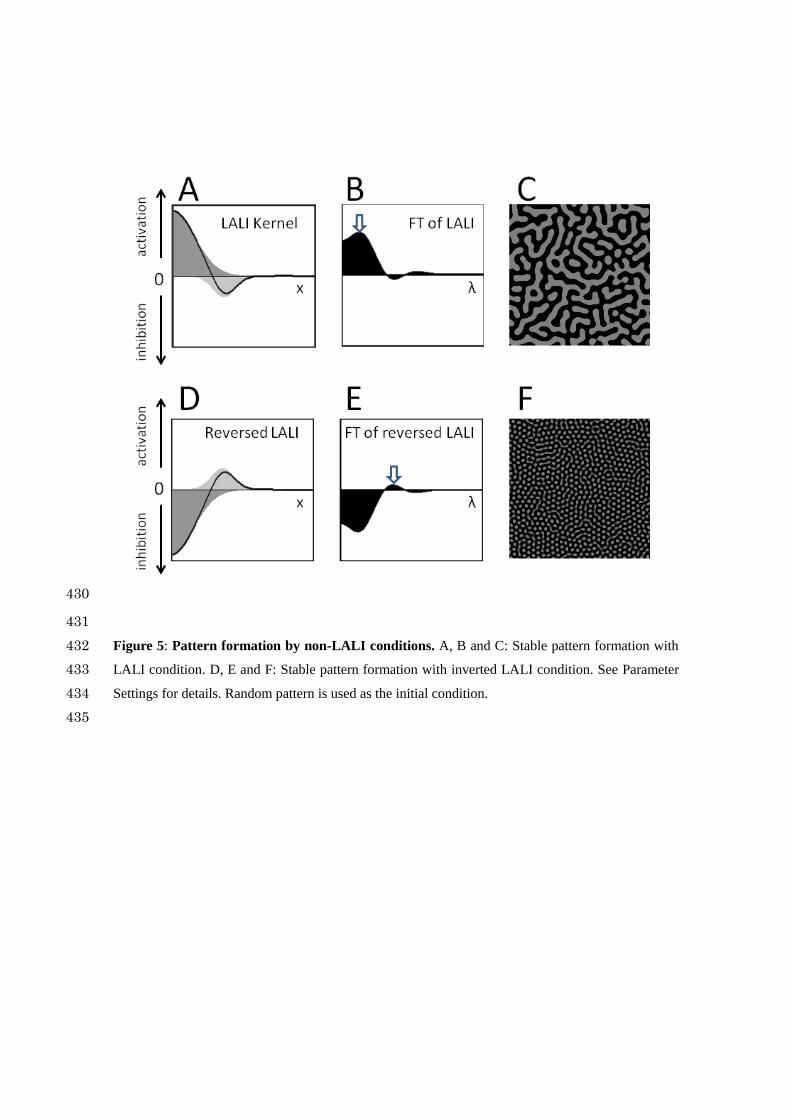
Pattern formation by variations on LALI conditions 167

I next examined pattern formation when the peak position of I(x) was offset from 0 (Figure 5A). This 168

condition also satisfies LALI, and a periodic pattern emerged as in the classical LALI model (Figure 169

5B and C). 170

171

Next, by exchanging the A(x) and I(x) functions, I established an inverted LALI condition that has 172

not been tested in the previous study of LALI models (Figure 5D). This inverted LALI condition 173

gave rise to a periodic pattern with a smaller wavelength (Figure 5F). The reason is clear from the 174

FT graph; by setting the peak position larger than zero, the FT graph shows a wave pattern. Inversion 175

of the kernel causes the emergence of a new peak at a different position (Figure 5B and E, arrows). 176

We can conclude from this result that LALI is not a necessary condition for the formation of periodic 177

patterns. 178

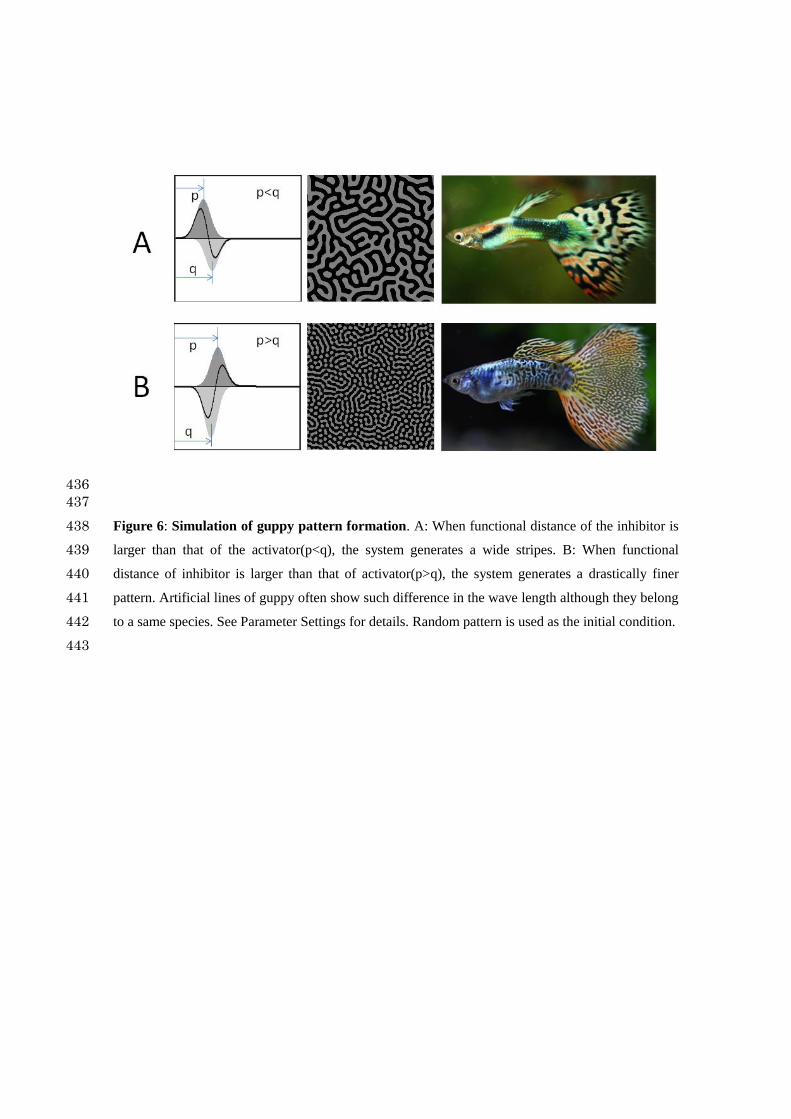
179

Some biological examples seem to correspond to this case. In some aquarium fish subjected to 180

selective breeding, the wavelength of the pigmentation pattern varies extensively among the breed 181

(Figure 6A, B). To account for this phenomenon with the conventional RD model requires setting 182

extremely different diffusion rates for each breed. However, because these fish belong to the same 183

species, the mechanism that forms the pattern should be almost the same, and therefore this 184

assumption is biologically quite unlikely. By assuming that the signal transduction has an effective 185

peak at a distant region from the source cell, it is possible to generate patterns of extensively 186

different wavelengths by making only slight changes to the parameter values. 187

188

Nested pattern formation 189

By setting the peak positions of both A(x) and I(x) distant from zero, the FT of the kernel shows a 190

wave pattern and multiple peaks emerge. When a 2D pattern is calculated with these conditions, in 191

most cases, the dominant wavelength dictates the pattern and thus a periodic pattern resembling that 192

with a single wavelength emerges (data not shown). However, by tuning the parameters, it is 193

possible to generate a nested pattern with two or more wavelengths (Figure 7A, B, and C). 194

Interestingly, very similar nested patterns are found in some fish species (Figure 7D, E). 195

196

Identification of the primary factor that determines the variety of 2D patterns 197

The RD and other LALI models are able to generate a variety of 2D patterns, namely spots, stripes, 198

and networks, and previous studies have examined the parameter sets that give rise to these patterns 199

for each specific model. However, because each model is built on different assumptions of the 200

behaviours of molecules and cells, little is known about the primal factor that controls the 2D 201

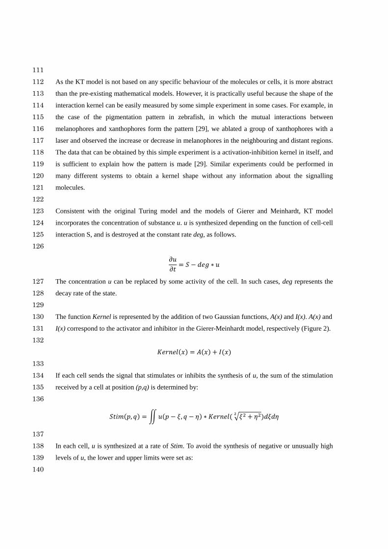
pattern. 202

203

I tested a number of different kernel shapes with the KT model, and in all cases, the determinant of 204

the 2D shape of the waves was the integrated value of the 2D kernel. By setting the integrated value 205

close to zero, stripe patterns emerge irrespective of the kernel shape, while spots always emerge at 206

smaller integrated values and inverted spots (networks) emerge with larger integrated values (Figure 207

8A, B, and C). This result persisted when rectangular waves, trigonometric functions, or polygonal 208

lines were used as the kernel shape. This strongly suggests that the primal factor that determines the 209

shape of the 2D wave pattern is the integrated value of the kernel function. 210

211

Discussion 212

213

Unlike the RD and other LALI models, the KT model does not assume any mechanisms of 214

molecules or cells, but directly uses an input activation-inhibition kernel. Because of its abstract 215

nature, the KT model cannot predict the detailed molecular or cellular processes involved in the 216

pattern formation. However, as shown in this report, the kernel shape itself provides enough 217

information to explain the formation of various stable patterns. Moreover, the simplicity of the KT 218

model confers some significant advantages that complement the shortcomings of conventional 219

mathematical models. 220

221

Usage of the KT model in experimental studies 222

Different LALI models that postulate different molecular or cellular mechanisms can sometimes 223

form very similar patterns. Therefore, even if a biological pattern is reproduced by the simulation of 224

a specific LALI model, it does not guarantee that the molecular mechanism anticipated in the model 225

underlies the biological system. Even with recent advances in technology and experimental methods, 226

it is still difficult to identify every part of a molecular network that is involved in formation of a 227

biological pattern. Especially at the beginning of an experimental project, little molecular 228

information is usually available. In most cases, therefore, it is quite difficult to construct a 229

pattern-formation simulation on the basis of reasonable experimental data. These problems led 230

Greene and Economou to question the efficacy of RD and LALI models in the experimental research 231

of morphogenesis[22]. 232

233

As the KT model is not based on any specific molecular mechanism, it likewise cannot be used to 234

make molecular-level predictions. However, KT model simulations can be performed with a 235

sufficient experimental basis because it is easier to detect the kernel shape. For example, the 236

pigmentation pattern of zebrafish skin is generated by an array of black melanophores and 237

xanthophores that mutually interact. Using laser ablation to kill the cells in a particular region, we 238

measured the increase and decrease of cell density at nearby and distant regions [29]. The data 239

obtained from this simple experiment is the kernel itself, which is sufficient to predict the 240

development of 2D patterns. In that previous paper[29], we used the conventional RD model. 241

However, it was later discovered that the signals are not transferred by diffusion but by the direct 242

contact of cell projections. Because the condition of LALI is retained by both types of projections 243

(long and short), the predictions made by the simulation were correct. However, using an RD model 244

for a system that does not involve diffusion is theoretically contradictory. Using kernel-based 245

simulation can avoid this problem. Kernel detection is also feasible in many other systems. Using 246

light-gated channels or infrared light, for example, one can stimulate, inhibit, or kill cells located at 247

an arbitrary region, and observe the subsequent changes in surrounding cells by live-cell imaging. 248

Therefore, in many cases where the detailed molecular mechanism is unknown, using the KT model 249

should still be safe and practical. 250

251

Usage of the KT model in theoretical analysis 252

In a simple RD model with two substances, the necessary conditions for stable pattern formation are 253

analytically induced. However, the number of elements (molecules and cells) involved in real 254

pattern-formation events usually far exceeds two. In such cases, the applicability of the LALI 255

concept is uncertain. In fact, some recent computational studies reported that mathematical models 256

of three substances were able to form stable periodic patterns using the reversed LALI condition [30] 257

[31]. Therefore, the concept of LALI is likely not sufficient to analyse a realistic system with more 258

than three factors. To identify more generalized conditions for the pattern formation, mathematical 259

unification of the various patterning mechanisms may be required. As Murray suggested [4], the 260

kernel concept may be useful for this unification. As shown in this report, the variety of 2D patterns 261

generated by the KT model is wide enough to cover most known biological patterns. Patterns formed 262

by the reversed LALI condition[30, 31] can also be reproduced by the KT model. Moreover, the 263

simulation result of KT model(figure7) shows that it can generate some complex spatial patterns that 264

is difficult to be made by conventional models. Nested patterns appear often on the animal skin and 265

sea shells. To reproduce such patterns, conventional models needed to combine two sets of Turing 266

systems[32] or to function a RD system twice with a time lag[33]. With the KT model, adjusting the 267

two Gaussian functions is, however, enough to generate such patterns, and the reason why the nested 268

patterns emerges is clear from the FT of the kernel shape. Therefore, if it is possible to translate the 269

property of a given molecular network into a kernel shape, the behaviours of different models can be 270

addressed in a unified method. 271

272

According to the simulation results from the KT model (Figures 4, 5, and 6), the conditions of stable 273

pattern formation are quite simple: the integrated value of the 2D kernel is near zero, and the FT of 274

the kernel has upward peaks. Concerning to the variety of the 2D pattern, Gierer and Meinhardt 275

suggested that the saturation of activator synthesis is the key to change the spots to stripe and 276

network [3]. However, this suggestion was not tested with rigorous mathematical analysis. With the 277

KT model, the type of 2D pattern generated (spots, stripes, or networks) depends almost entirely on 278

the integrated value of the 2D kernel. Although more mathematically strict verification should be 279

performed in future studies, these simple conditions would be useful to understand the principle of 280

pattern formation in real systems. 281

282

The properties of the KT model described above can complement the weaknesses identified in the 283

pre-existing mechanistic models for autonomous pattern formation. I hope that the kernel-based 284

method presented here will contribute to the progression of our understanding of biological pattern 285

formation. 286

287

Acknowledgement 288

I thank professors Takeshi Miura, Yoshihiro Tanaka and Ei Shin-ichiro for critical discussions and 289

suggestions. 290

291

Funding 292

This study was supported by JST, CREST and MEXT, Grant-in-Aid for Scientific Research on 293

Innovative Areas. 294

295

Simulation program and the parameter sets used in the study 296

297

The simulation program was coded with Processing2.0 (Massachusetts Institute of Technology). 298

The compiled program will be distributed from the journal HP and the institute HP of Kondo. 299

The kernel function was defined as follows, where x is the distance between the cells: 300

301

Kernel[x] = ActivatorKernel[x] + InhibitorKernel[x] 302

ActivatorKernel[x] = ampA/sqrt(2*PI)*exp(-(sq((x-distA)/widthA)/2)) 303

InhibitorKernel[x] = ampI/sqrt(2*PI)*exp(-(sq((x-distI)/widthI)/2)) 304

305

The six parameters (ampA, ampI, widthA, widthI, dispA, and dispI) that determine the shape of the 306

kernel are changed by the control sliders. The FT of the kernel, 3D kernel shape, and integrated 307

value of the 2D kernel are automatically calculated when the parameter values are changed. 308

Pushing the “start-calculation” and “stop-calculation” buttons starts and stops the calculation, 309

respectively. The “random-pattern” button gives a random value (0~1) to each cell. The 310

“clear-the-field” button gives a value of 0 to each cell. Clicking the mouse on the calculation field 311

gives a value of 0.5 to the cell at the position of the cursor. 312

313

Parameter Settings 314

ampA ampI widthA widthI distA distI 2D

integrat

ed

Fig. 4C left 20.267 -2.133 1.817 5.835 0 0 -14.119

Fig. 4C centre 21.971 -2.133 1.817 5.835 0 0 -0.017

Fig. 4C right 250.67 -2.133 1.817 5.835 0 0 25.604

Fig. 5 upper 22.4 -8 2.748 1.278 0 6.7 -0.398

Fig. 5 lower -22.4 8 2.748 1.278 0 67 -0.398

Fig. 6A 15.275 -11.733 1.082 0.886 4.4 7 -0.318

Fig. 6B 12.656 -18.133 1.082 0.886 6.8 5.799 -0.413

Fig. 7A 17.192 -13.333 1.18 1.18 8.3 10.7 0.2

Fig. 7B 21.085 -19.733 0.739 0.935 10.3 8.7 -0.158

Fig. 7C 16.869 -5.867 1.229 3.872 5.9 6.1 24.6

Fig. 8A 20 14.287 -3.733 2.601 4.855 0 0 21.642

Fig. 8A 10 13.61 -3.733 2.601 4.855 0 0 10.246

Fig. 8A 0 13 -3.733 2.601 4.855 0 0 -0.11

Fig. 8A -10 12.413 -3.733 2.601 4.855 0 0 -10.59

Fig. 8A -20 11.827 -3.733 2.601 4.855 0 0 -20.001

Fig. 8B 40 13.652 -7.466 0.886 5.835 8.9 0 39.96

Fig. 8B 20 13.251 -7.466 0.886 5.835 8.9 0 20.076

Fig. 8B 0 12.844 -7.466 0.886 5.835 8.9 0 -0.072

Fig. 8B -20 12.443 -7.466 0.886 5.835 8.9 0 -19.956

Fig. 8B -40 12.038 -7.466 0.886 5.835 8.9 0 -39.97

Fig. 8C 40 14.182 -11.733 2.013 1.18 5.78 11.5 40.18

Fig. 8C 20 13.908 -11.733 2.013 1.18 5.78 11.5 20.032

Fig. 8C 0 13.634 -11.733 2.013 1.18 5.78 11.5 -0.022

Fig. 8C -20 13.356 -11.733 2.013 1.18 5.78 11.5 -20.468

Fig. 8C -40 13.089 -11.733 2.013 1.18 5.78 11.5 -40.034

315

316

References 317

318

[1] Turing, A. 1952 The Chemical Basis of Morphogenesis. Philosophical Transactions of the 319

Royal Society of London. Series B 237, 36. 320

[2] Meinhardt, H. 1995 Dynamics of stripe formation. 376, 2. 321

[3] Meinhardt, H. 1982 Models of biological pattern formation. London, Academic Press. 322

[4] Murray, J. 2001 Matheatical Biology. USA, Spriger. 323

[5] Gierer, A. & Meinhardt, H. 1972 A theory of biological pattern formation. Kybernetik 12, 324

30-39. 325

[6] Wearing, H.J., Owen, M.R. & Sherratt, J.A. 2000 Mathematical modelling of juxtacrine 326

patterning. Bulletin of mathematical biology 62, 293-320. (doi:10.1006/bulm.1999.0152). 327

[7] Swindale, N.V. 1980 A model for the formation of ocular dominance stripes. Proceedings 328

of the Royal Society of London. Series B, Biological sciences 208, 243-264. 329

[8] Belintsev, B.N., Beloussov, L.V. & Zaraisky, A.G. 1987 Model of pattern formation in 330

epithelial morphogenesis. J Theor Biol 129, 369-394. 331

[9] Budrene, E.O. & Berg, H.C. 1995 Dynamics of formation of symmetrical patterns by 332

chemotactic bacteria. Nature 376, 49-53. (doi:10.1038/376049a0). 333

[10] Oster, G.F. 1988 Lateral inhibition models of developmental processes. Mathematical 334

Biosciences 90, 256-286. (doi:10.1016/0025-5564(88)90070-3). 335

[11] Maini, P. 2004 The impat of Turing's work on pattern formation in biology. Mathematics 336

Today 40, 2. 337

[12] Blanchedeau, P., Boissonade, J. & De Kepper, P. 2000 Theoretical and experimental 338

studies of spatial bistability in the chlorine-dioxide-iodide reaction. Physica D 147, 17. 339

[13] Ouyang , Q. & Swinney, H. 1991 Transition from a uniform state to hexagonal and 340

striped Turing patterns. Nature 352, 3. 341

[14] Kondo, S. & Asal, R. 1995 A reaction-diffusion wave on the skin of the marine angelfish 342

Pomacanthus. Nature 376, 765-768. 343

[15] Yamaguchi, M., Yoshimoto, E. & Kondo, S. 2007 Pattern regulation in the stripe of 344

zebrafish suggests an underlying dynamic and autonomous mechanism. Proc Natl Acad Sci 345

U S A 104, 4790-4793. (doi:10.1073/pnas.0607790104). 346

[16] Hamada, H. 2012 In search of Turing in vivo: understanding Nodal and Lefty behavior. 347

Developmental cell 22, 911-912. (doi:10.1016/j.devcel.2012.05.003). 348

[17] Maini, P.K., Baker, R.E. & Chuong, C.M. 2006 Developmental biology. The Turing model 349

comes of molecular age. Science (New York, N.Y.) 314, 1397-1398. 350

(doi:10.1126/science.1136396). 351

[18] Muller, P., Rogers, K.W., Jordan, B.M., Lee, J.S., Robson, D., Ramanathan, S. & Schier, 352

A.F. 2012 Differential diffusivity of Nodal and Lefty underlies a reaction-diffusion 353

patterning system. Science (New York, N.Y.) 336, 721-724. (doi:10.1126/science.1221920). 354

[19] Sheth, R., Marcon, L., Bastida, M.F., Junco, M., Quintana, L., Dahn, R., Kmita, M., 355

Sharpe, J. & Ros, M.A. 2012 Hox genes regulate digit patterning by controlling the 356

wavelength of a Turing-type mechanism. Science (New York, N.Y.) 338, 1476-1480. 357

(doi:10.1126/science.1226804). 358

[20] Kondo, S. & Miura, T. 2010 Reaction-diffusion model as a framework for understanding 359

biological pattern formation. Science (New York, N.Y.) 329, 1616-1620. 360

(doi:10.1126/science.1179047). 361

[21] Green, J.B. & Sharpe, J. 2015 Positional information and reaction-diffusion: two big 362

ideas in developmental biology combine. Development 142, 1203-1211. 363

(doi:10.1242/dev.114991). 364

[22] Economou, A.D. & Green, J.B. 2014 Modelling from the experimental developmental 365

biologists viewpoint. Semin Cell Dev Biol 35, 58-65. (doi:10.1016/j.semcdb.2014.07.006). 366

[23] Hamada, H., Watanabe, M., Lau, H.E., Nishida, T., Hasegawa, T., Parichy, D.M. & 367

Kondo, S. 2014 Involvement of Delta/Notch signaling in zebrafish adult pigment stripe 368

patterning. Development 141, 318-324. (doi:10.1242/dev.099804). 369

[24] Inaba, M., Yamanaka, H. & Kondo, S. 2012 Pigment pattern formation by 370

contact-dependent depolarization. Science (New York, N.Y.) 335, 677. 371

(doi:10.1126/science.1212821). 372

[25] Yamanaka, H. & Kondo, S. 2014 In vitro analysis suggests that difference in cell 373

movement during direct interaction can generate various pigment patterns in vivo. Proc 374

Natl Acad Sci U S A 111, 1867-1872. (doi:10.1073/pnas.1315416111). 375

[26] De Joussineau, C., Soule, J., Martin, M., Anguille, C., Montcourrier, P. & Alexandre, D. 376

2003 Delta-promoted filopodia mediate long-range lateral inhibition in Drosophila. Nature 377

426, 555-559. (doi:10.1038/nature02157). 378

[27] Sagar, Prols, F., Wiegreffe, C. & Scaal, M. 2015 Communication between distant 379

epithelial cells by filopodia-like protrusions during embryonic development. Development 380

142, 665-671. (doi:10.1242/dev.115964). 381

[28] Vasilopoulos, G. & Painter, K.J. 2016 Pattern formation in discrete cell tissues under 382

long range filopodia-based direct cell to cell contact. Math Biosci 273, 1-15. 383

(doi:10.1016/j.mbs.2015.12.008). 384

[29] Nakamasu, A., Takahashi, G., Kanbe, A. & Kondo, S. 2009 Interactions between 385

zebrafish pigment cells responsible for the generation of Turing patterns. Proc Natl Acad Sci 386

U S A 106, 8429-8434. (doi:10.1073/pnas.0808622106). 387

[30] Marcon, L., Diego, X., Sharpe, J. & Muller, P. 2016 High-throughput mathematical 388

analysis identifies Turing networks for patterning with equally diffusing signals. Elife 5. 389

(doi:10.7554/eLife.14022). 390

[31] Miura, T. 2007 Modulation of activator diffusion by extracellular matrix in Turing 391

system. RIMS Kyokaku Bessatsu B3, 12. 392

[32] Meinhardt, H. 2009 The Algorithmic Beauty of Sea Shells, Springer-Verlag Berlin 393

Heidelberg. 394

[33] Liu, R.T., Liaw, S.S. & Maini, P.K. 2006 Two-stage Turing model for generating pigment 395

patterns on the leopard and the jaguar. Physical review. E, Statistical, nonlinear, and soft 396

matter physics 74, 011914. (doi:10.1103/PhysRevE.74.011914). 397

398

399

Figure legends 400

401

402

403

Figure 1: Interaction strength profiles depend on the method of signal transfer. A: In case of the 404

signal by diffusion, the interaction strength is highest at the source(cell) position. B: If the signal 405

molecule is released at the specific position of a cell projection, the peak of the interaction strength is 406

distant from the source(cell) position. 407

408

409

410

Figure 2: Definition of the Kernel shape. Kernel function is determined by the addition of two 411

Gaussian functions that can be modified by three parameters: amplitude(ampA and ampB), 412

width(widthA and widthB) and distribution (distA and distB). 413

414

415

416

Figure 3: Display of the KT model simulator. User can change the parameters of two Gaussians 417

with slider controller. The program automatically calculates and shows the 1D and 2D kernel, and 418

the FT of the kernel. Resulting 2D pattern is shown in the big 2D window. 419

420

421

422

Figure 4: Pattern formation by LALI conditions. A: The graph of the kernel that s equivalent to 423

the condition of LALI. Gaussian distribution for activator and inhibitor are represented by dark gray 424

and light gray pattern. The kernel (addition of two Gaussians) is represented by the black line. B: 425

Fourier transform of the kernel. Arrow indicates the peak position that represents the spatial 426

frequency of emerging pattern. C: Generated patterns with slightly different parameter sets. (see 427

Parameter Settings for details). Random pattern is used as the initial condition. 428

429

430

431

Figure 5: Pattern formation by non-LALI conditions. A, B and C: Stable pattern formation with 432

LALI condition. D, E and F: Stable pattern formation with inverted LALI condition. See Parameter 433

Settings for details. Random pattern is used as the initial condition. 434

435

436

437

Figure 6: Simulation of guppy pattern formation. A: When functional distance of the inhibitor is 438

larger than that of the activator(p<q), the system generates a wide stripes. B: When functional 439

distance of inhibitor is larger than that of activator(p>q), the system generates a drastically finer 440

pattern. Artificial lines of guppy often show such difference in the wave length although they belong 441

to a same species. See Parameter Settings for details. Random pattern is used as the initial condition. 442

443

444

445

Figure 7: Nested patterns generated by the KT model and examples of nested patterns in the 446

skin of fish. A, B and C: Three different types of the kernels and the resulting patterns. D: An 447

artificial line of guppy. E: Japanese common eel. See Parameter Settings for details. Random pattern 448

is used as the initial condition. 449

450

451

452

Figure 8: Relationship between the integrated values of the 2D kernel (noted above each 453

pattern) and the generated pattern. Five resulting 2D patterns calculated with the integrated 454

values (upper) are shown for the kernel A, B and C. With this small difference of the integrated 455

values of 2D kernel, the graph of FT and Kernel(x) looks almost identical. FT: Fourier Transform of 456

the kernel shapes. For the Gaussian parameters of each kernel, see the list of parameter settings. 457

458