Embed Size (px)
Citation preview

San Jose State University San Jose State University
SJSU ScholarWorks SJSU ScholarWorks
Master's Theses Master's Theses and Graduate Research
Fall 2014
An Unsaturated Zone Flux Study in a Highly-fractured Bedrock An Unsaturated Zone Flux Study in a Highly-fractured Bedrock
Area: Ground Water Recharge Processes at the Masser Recharge Area: Ground Water Recharge Processes at the Masser Recharge
Site, East-central Pennsylvania Site, East-central Pennsylvania
Zhengzheng Qin San Jose State University
Follow this and additional works at: https://scholarworks.sjsu.edu/etd_theses
Recommended Citation Recommended Citation Qin, Zhengzheng, "An Unsaturated Zone Flux Study in a Highly-fractured Bedrock Area: Ground Water Recharge Processes at the Masser Recharge Site, East-central Pennsylvania" (2014). Master's Theses. 4512. DOI: https://doi.org/10.31979/etd.gzj3-pdx2 https://scholarworks.sjsu.edu/etd_theses/4512
This Thesis is brought to you for free and open access by the Master's Theses and Graduate Research at SJSU ScholarWorks. It has been accepted for inclusion in Master's Theses by an authorized administrator of SJSU ScholarWorks. For more information, please contact [email protected].

AN UNSATURATED ZONE FLUX STUDY IN A HIGHLY-FRACTURED
BEDROCK AREA: GROUND WATER RECHARGE PROCESSES AT THE
MASSER RECHARGE SITE, EAST-CENTRAL PENNSYLVANIA
A Thesis
Presented to
The Faculty of the Department of Geology
San José State University
In Partial Fulfillment
of the Requirements for the Degree
Masters of Science
by
Zhengzheng Qin
December 2014

© 2014
Zhengzheng Qin
ALL RIGHTS RESERVED

The Designated Thesis Committee Approves the Thesis Titled
AN UNSATURATED ZONE FLUX STUDY IN A HIGHLY-FRACTURED
BEDROCK AREA: GROUND WATER RECHARGE PROCESSES AT THE
MASSER RECHARGE SITE, EAST-CENTRAL PENNSYLVANIA
by
Zhengzheng Qin
APPROVED FOR THE DEPARTMENT OF GEOLOGY
SAN JOSÉ STATE UNIVERSITY
December 2014
Dr. June A. Oberdorfer Department of Geology
Dr. Emmanuel Gabet Department of Geology
Dr. John R. Nimmo U.S. Geological Survey

ABSTRACT
AN UNSATURATED ZONE FLUX STUDY IN A HIGHLY-FRACTURED
BEDROCK AREA: GROUND WATER RECHARGE PROCESSES AT THE
MASSER RECHARGE SITE, EAST-CENTRAL PENNSYLVANIA
By Zhengzheng Qin
This study tested the applicability of the Episodic Master Recession method
and utilized the source-responsive flow theory to quantify ground water recharge and
simulate preferential flow in the vadose zone at the Masser Recharge Site in east-
central Pennsylvania. The ground water recharge shows strong seasonal variations.
The shallow fractures form preferential flow paths and predominate in the vadose
zone recharge processes, as reflected in the ground water-table elevation rise. They
also influence the ground water-table recession rate, reflected in the rapid water-table
recession in the deeper well with a high hydraulic conductivity fractured zone. Most
importantly, the source-responsive flow model was able to predict closely the well
water-level fluctuation over six months of wet-season recharge events with
parameters assigned to this site. The calibrated parameters are reasonable for the
fracture frequency and can serve as basis for predictions when applied to the
following wet-season precipitation record.

ACKNOWLEDGEMENTS
Dr. John R. Nimmo raised the key hypotheses for both the Episodic Master
Recession method and the source-responsive flow model. Dr. Gordon J. Folmar
from Agriculture Research Services of United States Department of Agriculture
(USDA-ARS) provided all the field data from the Masser site. Charles Horowitz
and Lara Mitchell developed the Matlab scripts for the Episodic Master Recession
method. I also thank Kimberlie S. Perkins for her helping evaluating the source-
responsive model results and for giving me good suggestions. I’m grateful to Dr.
June Oberdorfer for guiding and reviewing all my work.
v
TABLE OF CONTENTS
INTRODUCTION ......................................................................................................... 1
BACKGROUND ........................................................................................................... 3
Model ....................................................................................................................... 3
Field Site description ............................................................................................... 7
Field data ................................................................................................................ 10
METHODS .................................................................................................................. 14
Master Recession Curve ........................................................................................ 15
Source-Responsive Flow Model ............................................................................ 16
Episodic Master Recession Method ....................................................................... 20
Parameter Identification ......................................................................................... 23
Specific Yield .................................................................................................. 23
Ground Water-Table Recession Constants ..................................................... 24
Macropore Facial Area Density ..................................................................... 24
Active Area Fraction and Infiltration Capacity .............................................. 25
Lag Time ......................................................................................................... 25
Storm Recovery Time ...................................................................................... 26
Water-Table Fluctuation Tolerance ............................................................... 27
RESULTS .................................................................................................................... 29
MRC Evaluation .................................................................................................... 29
Calibration and Application of the Source-Responsive Flow Model .................... 31
EMR Method ......................................................................................................... 36
DISCUSSION .............................................................................................................. 41
Effects of Geological Factors ................................................................................. 41
Seasonal and Episodic Variations .......................................................................... 44
Sources of Uncertainty ........................................................................................... 47
vi
CONCLUSIONS.......................................................................................................... 51
REFERENCES CITED ................................................................................................ 53
APPENDIX A: MRC Fitted Curves ............................................................................ 55
APPENDIX B: Source-Responsive Model Sensitivity Analysis ................................ 60
APPENDIX C: Source-Responsive Model Calibration Plots ...................................... 67
APPENDIX D: EMR Output Plots .............................................................................. 73
APPENDIX E: EMR Output Tables ............................................................................ 80
vii

LIST OF FIGURES
Figure
1. Elevation Elements of a Water-table-fluctuation Study. ......................................... 7
2. Map of the Study Area ............................................................................................. 8
3. Fracture Patterns. ..................................................................................................... 9
4. Fracture Frequency with Depth for Rock Core ...................................................... 13
5. The Ground Water-Table Level in the NE, NW, and the CE Wells ...................... 18
6. Example of a Contour Plot Illustrating the Sensitivity Analysis of Mlim and Qcap 20
7. Example of an MRC Curve Fitted to the dH/dt vs. H Plot. ................................... 22
8. A Recharge Episode Graph Illustrating the EMR Method. ................................... 26
9. The Fluctuation Tolerance (δT) .............................................................................. 27
10. The MRC Fitted Curve ........................................................................................ 30
11. Contours Illustrating the Results of a Sensitivity Analysis ................................. 32
12. Comparison between the Observed Well Water-table Elevation and the Predicted
Well Water-table Elevation ........................................................................................ 34
13. Application of the Source-Responsive Model ..................................................... 35
14. EMR Analysis for the Masser Site for the NE Well Data ................................... 38
15. The Average Temperature Curve for the Water Year From1997-98................... 40
16. Cross-section of the Observation Wells and Core for the Masser Site. ............... 42
17. A Sample Hydrograph. ........................................................................................ 43
18. Plots of RPR vs. Maximum Rainfall Intensity. .................................................... 45
viii

19. Plots of RPR vs. Average Rainfall Intensity. ....................................................... 45
20. The Cumulative Precipitation .............................................................................. 50
ix

LIST OF TABLES
Table
1. Properties of Ground Water Observation Wells. ................................................... 11
2. Results of Interval Packer Testing for Hydraulic Conductivity (K) ...................... 12
3. Example of Output Table from the EMR Code. .................................................... 22
4. MRC Fitted Curve Coefficients. ............................................................................ 30
5. τ and H0 Values in Different Periods of the Water Year 1997-98. ......................... 31
6. The Mlim and Qcap Values Estimated by Sensitivity Analysis. ............................... 33
7. Results of the EMR Analysis for the NE Well. ..................................................... 37
8. Comparison of RPRs .............................................................................................. 40
x

INTRODUCTION
Ground water recharge cannot be directly measured using field techniques;
thus, methods for simulating the flux in the unsaturated zone have been used by
researchers to estimate recharge processes. Two new methods, the source-
responsive flow model and the Episodic Master Recession (EMR) method, can
improve our understanding of certain types of hydrogeological relationships, the
relation of preferential flow and recharge to seasonality and other climate-related
conditions, and help to manage ground water basins.
The source-responsive flux model simulates how flow in the vadose zone
responds sensitively to the dynamic conditions of the source of water input (Nimmo,
2010). In the source-responsive theory, the preferential flow transports infiltrated
water films as laminar flow along the internal faces of macropore walls.
Considering the relationship between the velocity and the thickness of laminar flows,
the preferential flow should have a uniform rate when the water input is continuous
and ample. Thus, we can use a formula to simulate how variations in water input
and other hydrologic factors impact the amount and timing of recharge. Use of the
source-responsive flow model can help in characterizing subsurface properties related
to recharge. The EMR method (Nimmo et al., 2014) can be used to evaluate
questions such as how the intensity or the seasonality of precipitation impacts
1

preferential flow and leads to rapid responses at the ground water table. It can
estimate recharge from individual events throughout the year.
This study focused on the application of the source-responsive flow model for
an entire water year of monitoring data selected from observation well measurements
from the Masser site in east-central Pennsylvania. With evaluation of the hydraulic
well-testing results and rock core data for the site, the relationships between the
ground water recharge and the geologic characteristics of the Masser site can be
evaluated. Previous studies of ground water recharge utilized the source-responsive
model to make predictions for a single recharge episode (Nimmo, 2010). It is
important to test the applicability of this model to see if it can simulate the
unsaturated-zone fluxes and make reliable explanations for the observed water-table
fluctuations during longer periods. The application of the EMR method for the
Masser site permitted evaluation of the seasonal variations of ground water recharge
and also evaluation of the specific yield for the site. Moreover, the ground water-
table recession behavior at the Masser site can be characterized by using the master
recession curve (MRC), which gives parameter values to use with both the source-
responsive flow model and the EMR method.
2

BACKGROUND
Model
Diffuse flow is influenced mainly by capillarity and gravity. It can be
formulated according to the Darcy-Buckingham Law,
𝑞𝑞D(𝑧𝑧) = −𝐾𝐾(𝜃𝜃D) 𝜕𝜕𝜕𝜕𝜕𝜕𝜕𝜕
[1]
where qD is the flux density [LT-1], K is the unsaturated hydraulic conductivity [LT-1],
θD is volumetric water content of the diffuse-flow domain [-], Φ is the total potential
relevant to flow in the diffuse domain [L], and z is upward distance [L].
In some cases, the ground water table shows a fast response to a water-
infiltration event at the ground surface. This rapid response cannot be explained by
slow, diffusive flow but rather involves preferential flow. Preferential flow is
hydraulic transport via enhanced flow-paths that permits fast movement in the
unsaturated zone.
The source-responsive theory is one way to investigate the preferential flow
process. Changing conditions of rainfall, irrigation, or other water-infiltration events
leads to sensitive responses of the water table. The input water from the land surface
is thought to transfer to the underlying aquifer via free-surface films on macropore
walls with varying velocity and thickness. Since preferential flow is another mode
3

of recharge in addition to the diffuse flow, the relation of wetness and flow patterns
can be simply considered as
𝜃𝜃 = 𝜃𝜃𝐷𝐷 + 𝜃𝜃𝑆𝑆 [2]
and
𝑞𝑞 = 𝑞𝑞𝐷𝐷 + 𝑞𝑞𝑆𝑆 [3]
where θD and qD are the water content and flux density of the diffuse flow domain and
θS and qS correspond to the source-responsive domain. The equation for situations
with preferential flow would be a combination of Darcy-Buckingham law and laminar
film flow concepts (Nimmo, 2010),
𝑞𝑞(𝑧𝑧, 𝑡𝑡) = −𝐾𝐾(𝜃𝜃𝐷𝐷) 𝜕𝜕𝜕𝜕𝜕𝜕𝜕𝜕
+ 𝑓𝑓(𝑧𝑧, 𝑡𝑡)𝑞𝑞SMAX(𝑧𝑧). [4]
The dimensionless factor f(z,t) is the active area fraction (fraction of the macropore
surface area over which preferential flow is actively taking place), which ranges from
0 to 1, depending on the flow conditions in the preferential flow path. The
parameter qSMAX (z) is the maximum possible source-responsive flow that could occur
via macropores [LT-1].
In a previous study (Nimmo, 2010), film-flow concepts were assumed to obey
laminar flow principles and were represented by a mathematical framework:
𝑞𝑞𝑆𝑆(𝑧𝑧, 𝑡𝑡) = 𝑉𝑉𝑢𝑢𝐿𝐿𝑢𝑢𝑀𝑀(𝑧𝑧)𝑓𝑓(𝑧𝑧, 𝑡𝑡) [5]
and
𝑉𝑉𝑢𝑢 = 13𝑔𝑔𝑣𝑣𝐿𝐿𝑢𝑢2 [6]
4

where ν [L2T-1] is the kinematic viscosity of water (assuming a temperature of 20 ̊C,
equal to 10-6 m2s-1), and M(z) [L-1] is the macropore facial area density. The
macropore facial area density is the surface area per unit volume of possible
preferential flow paths. It describes the capacity for transmitting preferential flow
and remains constant over time. The characteristic film velocity Vu [L T-1] and film
thickness Lu [L] are related by the laminar film-flow relation so that the source-
responsive preferential flow is described as
𝑞𝑞𝑆𝑆 (𝑧𝑧, 𝑡𝑡) = 𝑉𝑉𝑢𝑢1.5�3 𝑣𝑣𝑔𝑔𝑀𝑀(𝑧𝑧)𝑓𝑓(𝑧𝑧, 𝑡𝑡). [7]
When simulating recharge and deep water-table fluctuations, the distribution
and characteristics of fluxes in the vadose zone are unknown. We consider that the
source-responsive flux qS (z, t) is integrated over the vertical profile, from the land
surface (zls) to the depth of the water table (zwt), so that variations in M and f(z,t) with
depth can be ignored for a given recharge event. The function M(z) can be replaced
by a constant value for the limiting macropore facial area density, Mlim, and only
temporal variations in f(zwt, t) are considered (Mirus and Nimmo, 2013). Functional
relations between the availability of the source of recharge SR (zls, t) and activity of
the preferential flow pathways to the water table f(zwt, t) reflect a lag time as
𝑡𝑡𝑙𝑙𝑙𝑙𝑔𝑔 = 𝜕𝜕𝑤𝑤𝑤𝑤− 𝜕𝜕𝑙𝑙𝑙𝑙𝑉𝑉𝑢𝑢
or 𝑉𝑉𝑢𝑢 = 𝜕𝜕𝑤𝑤𝑤𝑤−𝜕𝜕𝑙𝑙𝑙𝑙𝑡𝑡𝑙𝑙𝑙𝑙𝑙𝑙
[8]
such that
𝑓𝑓�𝑧𝑧𝑤𝑤𝑡𝑡, 𝑡𝑡 + 𝑡𝑡𝑙𝑙𝑙𝑙𝑔𝑔� ∝ 𝑆𝑆𝑆𝑆(𝑧𝑧𝑙𝑙𝑙𝑙, 𝑡𝑡). [9]
The basic formula relating recharge flux to water-table fluctuations is
5

∆𝐻𝐻∆𝑡𝑡
= 𝑞𝑞(𝜕𝜕𝑤𝑤𝑤𝑤,𝑡𝑡)𝑆𝑆𝑦𝑦
− 𝐻𝐻𝜏𝜏 [10]
where H is the hydraulic head [L] above the hydrologic base-level H0 [L], or the zero
recession elevation, which is the water-table elevation if no preferential flow recharge
occurred for a long time (Fig. 1). Sy is the specific yield [-], and τ is the linear
master recession constant [T], derived from site specific regression analysis (Heppner
and Nimmo, 2005; Heppner et al., 2007). For most observations of rapid water-table
response, diffuse recharge fluxes through the unsaturated matrix can be considered
negligible and are set to zero. Combining equation [7], [8] with [10] and assigning
the land surface (zls) as z = 0 produces an equation:
∆𝐻𝐻∆𝑡𝑡
=�𝑧𝑧𝑤𝑤𝑤𝑤𝑤𝑤𝑙𝑙𝑙𝑙𝑙𝑙
�1.5
�3𝑣𝑣𝑙𝑙𝑀𝑀𝑙𝑙𝑙𝑙𝑙𝑙𝑓𝑓(𝜕𝜕𝑤𝑤𝑤𝑤,𝑡𝑡)
𝑆𝑆𝑦𝑦− 𝐻𝐻
𝜏𝜏. [11]
For the application of this model, the solution in recursion form is
𝐻𝐻𝑖𝑖+1 = 𝐻𝐻𝑖𝑖 exp �𝑡𝑡𝑙𝑙−𝑡𝑡𝑙𝑙+1𝜏𝜏
� +�𝑧𝑧𝑤𝑤𝑤𝑤𝑤𝑤𝑙𝑙𝑙𝑙𝑙𝑙
�1.5
�3𝑣𝑣𝑙𝑙𝑀𝑀𝑙𝑙𝑙𝑙𝑙𝑙𝑓𝑓𝑙𝑙+1𝜏𝜏
𝑆𝑆𝑦𝑦�1 − 𝑒𝑒𝑒𝑒𝑒𝑒 �𝑡𝑡𝑙𝑙−𝑡𝑡𝑙𝑙+1
𝜏𝜏�� [12]
where Hi is the H at the time step of ti. This formula can be used to predict H for a
sequence of intervals. An exponential function, exp �𝑡𝑡𝑙𝑙−𝑡𝑡𝑙𝑙+1𝜏𝜏
�, is used to represent
the recession processes. This version was developed based on Nimmo’s (2010)
source-responsive flow model.
The water-table fluctuation method uses Sy to estimate recharge from
observations of water-table fluctuations (ΔH) in wells with the formula,
𝑆𝑆𝑒𝑒𝑅𝑅ℎ𝑎𝑎𝑎𝑎𝑎𝑎𝑒𝑒 = 𝑆𝑆𝑦𝑦 × ∆𝐻𝐻 [13]
6

Figure 1. Elevation elements of a water-table-fluctuation study.
This source-responsive model has been used in case studies at the Idaho
Nuclear Technology and Engineering Center (INTEC), Rainier Mesa (RM), and the
Masser Recharge Site to evaluate model utility and data needs (Mirus and Nimmo,
2013).
Field Site description
The Masser Recharge Site was established by the Agricultural Research
Service (ARS), US Department of Agriculture, with installations including five
ground water-monitoring wells (Fig. 2). It is located within the Valley and Ridge
Physiographic Province and within the Susquehanna River Basin (Gburek and
Folmar, 1999) in central Pennsylvania. This non-glaciated area has a temperate and
humid climate. The site is about 266 m above mean sea level. It is situated near
7

the top of a knoll which is about 1,000 m long in the east-west direction and 400 m
wide in the north-south direction.
Figure 2. Map of the study area showing the location, regional topography and instrumentation of the Masser Recharge Site (modified from Gburek and Folmar, 1999).
Soils over the site are classified as Calvin shaley silt loam and Hartleton
channery silt loam that contain a high percentage of coarse fragments. They are
shallow and well drained with moderately high permeability which results in little or
no surface runoff. The surface elevation difference of the five wells is less than 1.6
m. Figure 2 shows where the wells are located. The slope of the study area is
0.024-0.04. It is relatively flat so that the infiltration produced by precipitation on
this study area is uniform and not influenced by elevation differences.
The Masser Recharge Site is located on the northern flank of an east-plunging
anticline; it is underlain by Mississippian-age, fractured, quartzitic sandstones with
8

less resistant Devonian-age interbedded sandstones, siltstones and shales. The
bedrock layers are highly to moderately fractured at shallow depths (about 2-20 m
deep from the ground surface) as a result of stress relief fracturing (Wyrick and
Borchers, 1981). There are three fracture sets (Fig. 3) that are roughly orthogonal to
each other (Burton et al., 2002). One closely spaced (centimeters to decimeters),
north-dipping fracture set is parallel to the bedding planes. Another fracture set is
spaced cleavage, ranged from closely spaced (centimeters) to more widely spaced
(decimeters to meters), parallel to the east-west-striking axial plane of the anticline
structure. The third fracture set is subvertical and widely spaced (meters to tens of
meters) along the north-south direction, which is perpendicular to the other two
fracture sets.
Figure 3. Fracture patterns of the anticline structure near the Masser Recharge Site (modified from Burton et al., 2002).
9

The water table is 5-15 m below land surface in fractured sandstone with a
small specific yield (Sy ~ 0.01) (Gburek and Folmar, 1999). The highly fractured
nature of the bedrock results in its higher hydraulic conductivities (K) and lower
specific yield (Sy) than typical unconsolidated porous material (Gburek and Folmar,
1999). These fractures are the likely sites of preferential flow in the vadose zone and
the cause of rapid water-table response to water-infiltration events.
The reports of watershed WE-38, a 7.4 km2 ARS research facility which is
located about 1 km east of the Masser Recharge Site, show that the average annual
precipitation of that area is approximately 1,090 mm (Gburek and Folmar, 1999).
The frequent rainfall events provide continuous water recharge to the shallow water
table, and 60%-80% of the total stream flow comes from subsurface return flow.
The episodic recharge to the ground water is seasonal. It occurs during the late
autumn, winter and spring months and sometimes, when there is a large precipitation
event, during the summer growing season (Gburek et al., 1986).
Field data
In this study, I utilized the precipitation data, well water-level data, the drill
core results, hydraulic testing results, fracture analysis, and seismic data interpretation
from the Masser Recharge Site. Continuous rainfall data (from April 1994 to
December 2001) were obtained in inches at the meterological site (Fig. 2) at half-hour
10
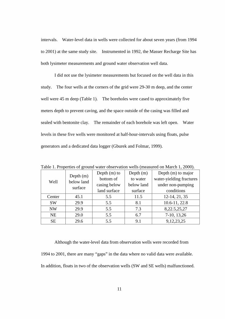
intervals. Water-level data in wells were collected for about seven years (from 1994
to 2001) at the same study site. Instrumented in 1992, the Masser Recharge Site has
both lysimeter measurements and ground water observation well data.
I did not use the lysimeter measurements but focused on the well data in this
study. The four wells at the corners of the grid were 29-30 m deep, and the center
well were 45 m deep (Table 1). The boreholes were cased to approximately five
meters depth to prevent caving, and the space outside of the casing was filled and
sealed with bentonite clay. The remainder of each borehole was left open. Water
levels in these five wells were monitored at half-hour-intervals using floats, pulse
generators and a dedicated data logger (Gburek and Folmar, 1999).
Table 1. Properties of ground water observation wells (measured on March 1, 2000).
Well Depth (m) below land
surface
Depth (m) to bottom of
casing below land surface
Depth (m) to water
below land surface
Depth (m) to major water-yielding fractures
under non-pumping conditions
Center 45.1 5.5 11.5 12-14, 21, 35 SW 29.9 5.5 8.1 10.6-11, 22.8 NW 29.9 5.5 7.3 8,22.5,25,27 NE 29.0 5.5 6.7 7-10, 13,26 SE 29.6 5.5 9.1 9,12,23,25
Although the water-level data from observation wells were recorded from
1994 to 2001, there are many “gaps” in the data where no valid data were available.
In addition, floats in two of the observation wells (SW and SE wells) malfunctioned.
11

I used data from two water years, October 1, 1997, to September 30, 1999, in the
center well (CE), the northeast well (NE), and the northwest well (NW) in this study.
Interval packer tests (Gburek and Folmar, 1999) were also conducted within
the five observation wells to determine hydraulic conductivity (K) values. Steady-
state, one-hole, double-packer tests were conducted on 3 m open intervals within each
well from below the casing to the bottom of the open borehole. K values of the open
interval (Table 2) were calculated based on well geometry and on flow rate and
pressure at steady state.
Table 2. Results of interval packer testing for hydraulic conductivity (K) (data from Gburek and Folmar, 1999).
Depth interval (m)
Fracture Layer K (m/day)
top bottom NW NE CE. SW SE Ave.
4.6 7.6 Highly
Fractured 0.62 0.75 1.8 high 2.16 1.3325 7.6 10.7
Moderately Fractured
0.32 0.23 0.16 0.36 2.9 0.794 10.7 13.7 0.18 0.03 0.07 1.5 0.28 0.412 13.7 16.8 0.52 0.03 0.33 0.11 0.14 0.226 16.8 19.8
Poorly Fractured (regional aquifer)
0.09 0.24 0.45 0.35 0.02 0.23 19.8 22.9 0.03 0.08 0.27 0.41 0.31 0.22 22.9 25.9 0.12 0.18 0.03 0.2 0.83 0.272 25.9 28.9 0.15 0.36 0.05 0.04 0.01 0.122 28.9 32 bottom bottom 0.03 bottom bottom 0.03 32 35 0.63 0.63 35 38.1 16.7 16.7
38.1 41.1 0.02 0.02 41.1 44.2 0.01 0.01
12
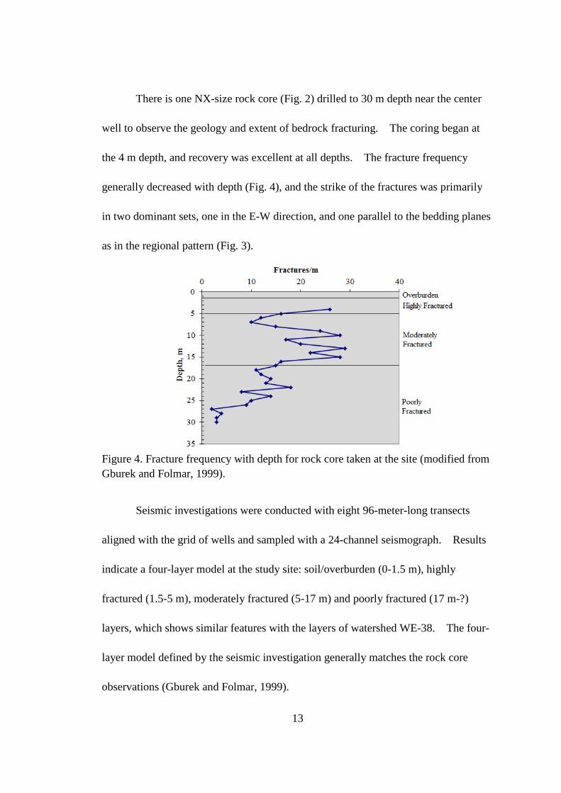
There is one NX-size rock core (Fig. 2) drilled to 30 m depth near the center
well to observe the geology and extent of bedrock fracturing. The coring began at
the 4 m depth, and recovery was excellent at all depths. The fracture frequency
generally decreased with depth (Fig. 4), and the strike of the fractures was primarily
in two dominant sets, one in the E-W direction, and one parallel to the bedding planes
as in the regional pattern (Fig. 3).
Figure 4. Fracture frequency with depth for rock core taken at the site (modified from Gburek and Folmar, 1999).
Seismic investigations were conducted with eight 96-meter-long transects
aligned with the grid of wells and sampled with a 24-channel seismograph. Results
indicate a four-layer model at the study site: soil/overburden (0-1.5 m), highly
fractured (1.5-5 m), moderately fractured (5-17 m) and poorly fractured (17 m-?)
layers, which shows similar features with the layers of watershed WE-38. The four-
layer model defined by the seismic investigation generally matches the rock core
observations (Gburek and Folmar, 1999).
13
METHODS
There were three major steps in the analysis of the water-level data from the
Masser Recharge Site. First, the recession periods were selected from the ground
water elevation data and used to create the MRC, which specifies the relationship
between the ground water-table decline rate (dH/dt) and the water-table elevation (H).
It can predict the dH/dt for a given well water-level elevation. Using an exponential-
decline model for the shape of the recession curve, this analysis also determines the
ground water-table recession constant (τ) and the base level (H0, the level the ground
water table would fall to without any episodic recharge). These two parameter
values can be used in estimating the parameters of the source-responsive flow model,
as well as in the application of the EMR method. Second is the calibration and
application of the source-responsive flow model. In this step, different parameters
that characterize the preferential flow and the ground water-table recession were
assigned and put into the source-responsive flow equation [12] to calibrate the model
to historic well water-level data. By conducting a global sensitivity analysis for
parameters such as Mlim and qcap using the available data from the NE, NW, and CE
well, the optimal parameters could be selected to simulate the data from each specific
well. Third, the EMR method was used to systematically partition well water-level
records and precipitation data into discrete time intervals of recharge and non-
recharge. The water-table fluctuation method was used to determine the beginning
14

and end of an individual recharge event (Nimmo et al., 2014). The advantage of the
episodic recharge approach is that it provides a method to determine the relationship
between water input and recharge for different precipitation events. The results help
in understanding the hydrodynamic behavior of the Masser site over the course of the
year. In this process, characteristics of each individual episode, such as the recharge
duration (h), recharge magnitude (m), precipitation duration (h), precipitation
magnitude (m), precipitation intensity (m/h), ground water-table rise (h), time lag (h),
and recharge to precipitation ratio (RPR) [-], are determined, verified, and compared
with other episodes.
Master Recession Curve
The MRC uses the water-table elevation data selected from the recession
periods for a specified time period to relate the rate of water-table decline (dH/dt)
with the water-table elevation (H). Given an MRC, one can predict the dH/dt as a
function of the current water-table elevation (Nimmo et al., 2014). In my study, I
utilized a Matlab code and an R code to pick out recession periods from times when
water levels were declining and then made a linear best-fit to the recession data
(dH/dt) as a function of water-table elevation (H). The scripts for this process are
called mrc_create. The input parameters include the polynomial degree to be used in
fitting the recession curve and the rain delay value. The output file gives the
15

coefficients of the formula that represent the MRC. Using a first-degree polynomial,
that is, a linear fit, the formula of the MRC is
𝑑𝑑𝐻𝐻 ∕ 𝑑𝑑𝑡𝑡 = 𝑃𝑃[0] + 𝑃𝑃[1] × 𝐻𝐻 [14]
where P[0] and P[1] are the coefficients (the y-intercept and the slope of the MRC,
respectively), and H is the relative well water level expressed as the height above the
base level (in meters). In the exponential form of the resulting H(t) formula [12], the
exponential decline constant τ and the zero recession elevation H0 are
𝜏𝜏 = −1 ∕ 𝑃𝑃[1] [15]
and
𝐻𝐻0 = −P[0] ∕ P[1]. [16]
Both the R version and the Matlab version were created by Lara Mitchell, who
worked with Dr. John R. Nimmo on preferential flow studies at the U.S. Geological
Survey in 2014.
Source-Responsive Flow Model
To gain a better understanding and verify the source-responsive flow theory,
precipitation data measured at the Masser Recharge Site were input into the source-
responsive model to calculate the water-table-elevation variations based on the
source-responsive flow equation [12]. Parameters that relate to the preferential flow
behavior of the unsaturated zone in generating recharge, such as Mlim (m-1), qcap
16

(mm/h), and tlag (h), and the parameters related to aquifer behavior, such as Sy [-] and
τ (h), were used at the same time.
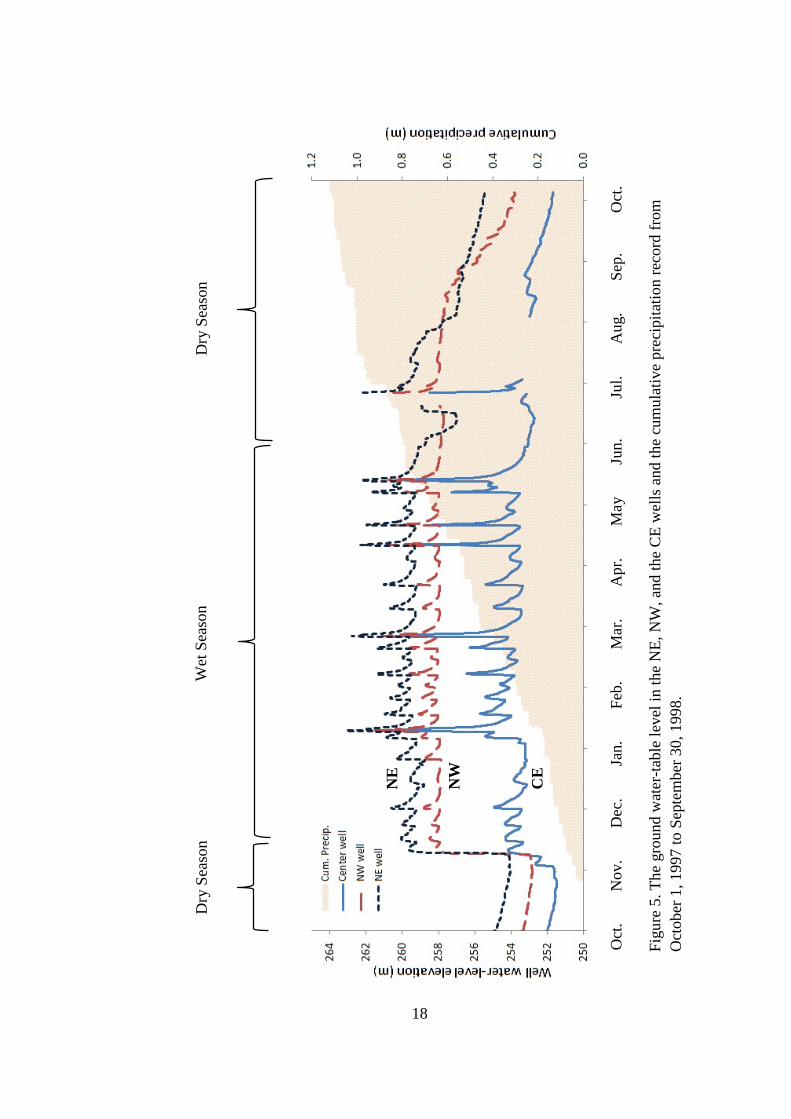
The data were separated into two major periods based on the ground water
level and the season (Fig. 5). Beginning in October 1997, the ground water table
was relatively low and kept declining, even when there were several precipitation
events, up to the middle of November 1997. At that point, the well water levels
suddenly rose more than five meters in the NW and the NE wells and about two
meters in the CE well. The base levels of the three observation wells remained at
relatively high elevations until May 1998. The well water levels slowly declined to
a lower base level after May 1998. Since the base water levels and the well level
behaviors varied greatly, the original data were analyzed separately and different
input parameters were used for these two periods. To distinguish these two periods
in this study, the one with relatively high ground water base levels and showing
frequent water-table fluctuations was called the “wet season” (November 16, 1997 to
May 15, 1998) while the rest of the year (October 1 to November 15, 1997 and May
16 to September 30, 1998) was called the “dry season”.
17
Wet
Sea
son
Oct
.
Nov
.
Dec
.
Jan
.
Feb
.
Mar
.
Apr
.
May
Jun.
Jul
.
Aug
.
Sep
.
O
ct.
Dry
Sea
son
Figu
re 5
. The
gro
und
wat
er-ta
ble
leve
l in
the
NE,
NW
, and
the
CE
wel
ls a
nd th
e cu
mul
ativ
e pr
ecip
itatio
n re
cord
from
O
ctob
er 1
, 199
7 to
Sep
tem
ber 3
0, 1
998.
NE
NW
CE
Dry
Sea
son
18

Considering the different behavior of the ground water table for the wet season
and for the dry season in all three observation wells, different parameters were
assigned in running the model calibration separately for each sets of data. By setting
up equations in an Excel worksheet and inputting the required parameters, predictions
of the water-table rise or decline based on precipitation amount per half-hour interval
were made beginning with an initial water-table elevation. The water level at the
subsequent time step was determined based on the simulated ΔH for each time step.
Before starting the calculation in Excel, it was necessary to determine the H0 and the τ
value for each well. Both parameters were determined by the MRC-fitted curve with
the equations [14], [15], and [16].
The basic concept in applying the source-responsive flow model was to use
one data set as a calibration sample. The calibrated parameters from that first data
set were then used in a second set of data collected from the same site to do a
verification simulation. As explained earlier, Mlim and f(t) are two parameters that
show porous medium characteristics and the preferential flow path availability,
respectively. These are the major factors influencing the modeled ground water
recharge processes. To evaluate the calibration, I calculated the root mean square
error (RMSE) for the difference between the observed well water level and the
simulated level. Sensitivity analyses for the Mlim and qcap (which controls f(t) value)
values were performed by varying those values within a reasonable range to get the
best estimations of both parameters (Fig. 6).
19

Figure 6. Example of a contour plot illustrating the sensitivity analysis of Mlim and qcap for the source-responsive flow model.
Episodic Master Recession Method
A recharge episode is considered as a period during which the total recharge
rate significantly exceeds its steady-state condition in response to a substantial water-
input event. Delineating an episode begins with estimating the MRC, which
represents the averaged recession behavior of an aquifer over a long period of time.
The method distinguishes episodes that have significantly greater recharge rates by
comparing the measured dH/dt curves with the MRC. With the output results from
the MRC, I used another Matlab code to identify individual recharge episodes based
on the water-table rise and the precipitation data. This EMR code is called
episodic_recharge.m and was also created by Lara Mitchell in 2013.
Mlim (m-1)
RMSE
q cap
(mm
/h)
20

Precipitation and well-response data at half-hour intervals from October 1997
to September 1998 were used for the analysis of responses at the CE well, the NW
well, and the NE well at the Masser site. Data measured in the SE and SW wells
were not used in this study since the floats in these two observation wells
malfunctioned. The data file for running the Matlab script must contain time (days),
the well water-level height above the zero recession elevation H0 (m), and the
cumulative precipitation with regular intervals (m). The polynomial order (zero to
third) to fit the MRC and the storm recovery time tp (days) should be included in the
input file to run the script. The output files from this script includes several graphs
such as a precipitation vs. time graph, a well water level vs. time graph, a dH/dt vs.
time graph, a dH/dt vs. well water level graph, and also the polynomial order and
coefficients of the fitted MRC curve (Fig. 7). Generally speaking, the higher the
polynomial order, the larger the coefficient of determination (R2). It is important to
find a balance between maximizing the R2 value and not letting the MRC fitted curve
become too complex.
The polynomial order and the coefficients determined by the MRC curve were
used as input parameters along with the fluctuation tolerance, lag time, and specific
yield to identify recharge episodes from the water level data sets in the EMR code.
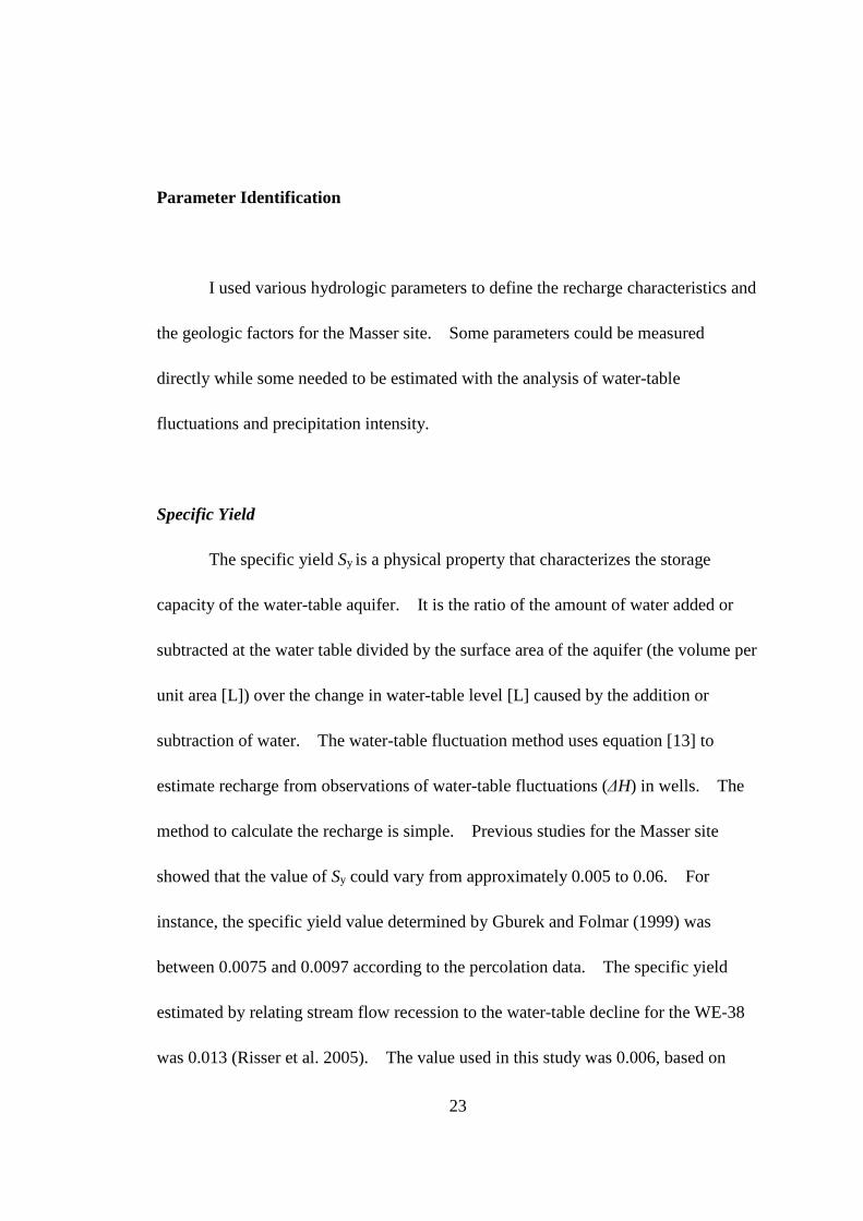
The EMR output includes a well water level vs. time graph, a dH/dt vs. time graph,
and a table with calculated precipitation and recharge features for each captured
episode (Table 3).
21
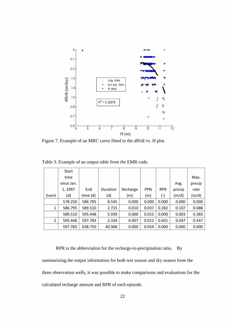
Figure 7. Example of an MRC curve fitted to the dH/dt vs. H plot.
Table 3. Example of an output table from the EMR code.
Event
Start time
since Jan. 1, 1997
(d) End
time (d) Duration
(d) Recharge
(m) PPN (m)
RPR (-)
Avg. precip (m/d)
Max. precip rate
(m/d) 578.250 586.795 8.545 0.000 0.000 0.000 0.000 0.000
1 586.795 589.510 2.715 0.010 0.037 0.282 0.107 0.688 589.510 595.448 5.939 0.000 0.015 0.000 0.003 0.383
2 595.448 597.783 2.334 0.007 0.012 0.601 0.047 0.447 597.783 638.750 40.968 0.000 0.054 0.000 0.000 0.000
RPR is the abbreviation for the recharge-to-precipitation ratio. By
summarizing the output information for both wet season and dry season from the
three observation wells, it was possible to make comparisons and evaluations for the
calculated recharge amount and RPR of each episode.
H (m)
dH/d
t (m
/day
)
22
Parameter Identification
I used various hydrologic parameters to define the recharge characteristics and
the geologic factors for the Masser site. Some parameters could be measured
directly while some needed to be estimated with the analysis of water-table
fluctuations and precipitation intensity.
Specific Yield
The specific yield Sy is a physical property that characterizes the storage
capacity of the water-table aquifer. It is the ratio of the amount of water added or
subtracted at the water table divided by the surface area of the aquifer (the volume per
unit area [L]) over the change in water-table level [L] caused by the addition or
subtraction of water. The water-table fluctuation method uses equation [13] to
estimate recharge from observations of water-table fluctuations (ΔH) in wells. The
method to calculate the recharge is simple. Previous studies for the Masser site
showed that the value of Sy could vary from approximately 0.005 to 0.06. For
instance, the specific yield value determined by Gburek and Folmar (1999) was
between 0.0075 and 0.0097 according to the percolation data. The specific yield
estimated by relating stream flow recession to the water-table decline for the WE-38
was 0.013 (Risser et al. 2005). The value used in this study was 0.006, based on
23

studies of previous recharge episodes and optimizing for a reasonable RPR value
(Nimmo et al, 2014).
Ground Water-Table Recession Constants
τ is a parameter representing the rate of water-table recession. It is the
amount of time required for a water table to decline a specific fraction of the range
between the initial water level and its base level (the fraction equals to 1-1/e, or
63.2%). It is a linear constant related to the rate of water-table decline. It was
assigned a value of 72 h for a case study at the Masser site (Nimmo, 2010). The
water-table recession rate is determined by the site characteristics and may range from
meters per day to meters per decade, which means the τ value may range from 24
hours to 87,600 hours (Mirus and Nimmo, 2013).
Macropore Facial Area Density
M [L-1] is a property of the porous medium, which represents the capacity for
transmitting preferential flow. It cannot be calculated or measured directly. Mlim is
the maximum surface area available for preferential flow per unit volume of porous
medium [L-1]. There should be a relationship between Mlim and the characteristics of
the hydrogeologic medium (e.g., porosity, Sy, fracture frequency, or particle size).
The range of Mlim values used in previous applications varied from 60 m-1 to 4000 m-1
(Nimmo, 2010). It is a constant parameter through time.
24

Active Area Fraction and Infiltration Capacity
The value of the active area fraction f(t) determines the available preferential
flow paths of the preferential-flow surface area (Mlim). It is assumed to be correlated
with the source of recharge, SR (zls,t), which represents records of precipitation,
infiltration, and/or stream-flow characteristics (e.g., precipitation intensity, duration,
and frequency). As described previously, the value of f(t) ranges from 0 to 1,
indicating what fraction of the macropore facial area is actively transmitting water.
Its value is determined by the amount of water percolating below the zone of
evapotranspiration. When calibrating the f(t) for the source-responsive flow model,
another coefficient, the infiltration rate needed to fully activate all preferential flow
paths (qcap), was used to relate the precipitation rate to the f(t) as
𝑓𝑓(𝑡𝑡) = 𝑅𝑅𝑙𝑙𝑖𝑖𝑅𝑅 𝐼𝐼𝑅𝑅𝑡𝑡𝐼𝐼𝑅𝑅𝑙𝑙𝑖𝑖𝑡𝑡𝑦𝑦𝑞𝑞𝑐𝑐𝑙𝑙𝑐𝑐
. [17]
The qcap is the maximum precipitation rate that can be absorbed at the land
surface without runoff. It is an adjustable parameter which is considered as a
transient value that is affected by the season and the soil moisture.
Lag Time
The lag time (tlag) is how long it takes for the source of recharge to transfer
from the land surface to the saturated zone and cause the ground water table to rise
(ΔH > 0), which is the time interval between the start of precipitation and the start of
25

the water-table rise (Fig. 8). The beginning of the recharge episode can be
determined by the EMR method. The lag time for a single episode event can be
determined by using a systematically applied criterion, which requires hydrologic
judgment to establish.
Figure 8. A recharge episode graph illustrating the EMR method. The red lines are extrapolations of the recession curves based on the MRC, the vertical distance ΔH represents the total actual water-table rise caused by the relevant rainfall event which began tlag days earlier.
From preliminary analysis between the precipitation data and the water-table
level data, the value of tlag could vary from a couple of hours to two to three days. I
used the average lag time in this study.
Storm Recovery Time
The minimum time between precipitation and recession, allowing for storm
generated accretion to become negligible, is called the storm recovery time (tp). The
MRC code can pick out recession data with a storm recovery time assigned to it.
ΔH
tlag
26

Water-Table Fluctuation Tolerance
A water-table fluctuation tolerance (δT) was used to distinguish recharge
periods from periods with non-significant water-table fluctuation rates, dH/dt (Figure
9). Since there are many small deviations that produce little recharge to the
saturated zone, considered as noise in the dH/dt time series, I used the fluctuation
tolerance to identify data within that noise range to be disregarded.
Figure 9. The fluctuation tolerance (δT) identified recharge periods (shown in darker blue) from insignificant variations in water level change rates. The blue area indicates cumulative precipitation.
When estimating the δT value, it should be large enough to eliminate the small
water elevation fluctuations while allowing the significant recharge events to be
clearly distinguished. My estimate of δT defined a band such that 90% of measured
recessionary dH/dt values fell within the band; this value could be adjusted if the
original δT designated unreasonable recharge episodes. For example, the δT value
δT
27

needed to be increased if it designated some minor or frequent episodes as
contributing positive recharge. On the other hand, it needed to be decreased if it
eliminated any major recharge episode. As shown in Figure 9, the bands are
determined by the fluctuation tolerance on either side of the recession curve. The
bolded curve represents dH/dt that crossed the upper fluctuation tolerance band which
means that a significant recharge event occurred.
28

RESULTS
Results for both the EMR method application and the source-responsive flow
model calibration showed variability in response to seasonal changes. Considering
the shifting vadose zone moisture state and the weather changes during the year, it is
reasonable to analyze the responses for different seasons separately.
MRC Evaluation
Considering the rate of water-table decline, dH/dT, to be proportional to the
head (H), with the result considered over time to be an exponential decline curve, the
polynomial order I used to get the MRC fitted coefficients was first-order. Having
determined the wet and dry periods in the observed records, I utilized the R script to
create the MRC fitted curve (example provided in Figure 10) and obtained fitted
coefficients for different periods in the water year 1997-98 as shown in Table 4. The
plots for all three wells in both seasons are provided in Appendix A. Investigations
using the MRC method showed that the ground water-level recession processes were
faster (dH/dT was greater) if H was greater (Fig. 10).
29

Figure 10. The MRC fitted curve shows the relationship between the dH/dt and the H for the wet-season data collected from the CE well in the water year 1997-98.
Table 4. MRC fitted curve coefficients.
Utilizing the equations [15] and [16], respectively, the τ value and H0 could be
calculated by using the MRC fitted coefficients for each of the three wells for the
different periods of the year (Table 5).
When comparing the various τ values in the different periods for the same
well, the dry season data indicated a larger τ (more gradual recession) than the wet
Period Well P[0] P[1] All water-year data (10/1/97-9/30/98
CE 20.947 -0.083 NE 4.207 -0.017 NW 3.745 -0.015
Wet season data (11/16/97-5/15/98)
CE 26.239 -0.104 NE 28.171 -0.109 NW 49.505 -0.192
Dry season data (10/1/97-11/15/97, 5/16/98-9/30/98)
CE 13.108 -0.052 NE 3.263 -0.013 NW 1.197 -0.005
30

season data. Among the three wells, the τ value changed much less in the CE well,
while it changed much more in the other two wells between the different data periods.
Table 5. τ and H0 values in different periods of the water year 1997-98.
Period Well τ (h) H0 (m) All year data
(10/1/97-9/30/98) CE 287.76 251.15 NE 1423.51 249.51 NW 1591.31 248.30
Wet season data (11/16/97-5/15/98)
CE 230.61 252.13 NE 219.93 258.15 NW 124.83 257.49
Dry season data (10/1/97-11/15/97, 5/16/98-9/30/98)
CE 457.26 249.74
NE 1820.40 247.47 NW 4786.98 238.67
Calibration and Application of the Source-Responsive Flow Model
Assigning H0 and τ values to each well according to values in Table 5 and 20 h
(the reasonable assumption for lag time) as tlag, a sensitivity analyses (Appendix B)
was run with the source-responsive flow model for different Mlim and qcap values (Fig.
11) to determine which combinations would produce the lowest RMSE value. M
and f(t) are strongly coupled with each other and determine the water-table responses
together. The qcap parameter inversely affects the magnitude of f(t) as shown in
equation [17]. It is likely that the Mlim and qcap have a specific optimal ratio. The
sensitivity analysis illustrates that the larger the Mlim assigned, the larger the qcap value
that needs to be utilized to minimize the RMSE. 31

Figure 11. Contours illustrating the results of a sensitivity analysis for the December 1997 - May 1998 period.
The result of sensitivity analyses showed that the potential Mlim value ranged
from 50 to 100 m-1, while the qcap value ranged from 10 to 70 mm/h. Since M has a
physical interpretation, representing the macropore facial area density of the medium,
it should be set to a unique value. While the Mlim value should be held constant
across the seasons, qcap varies seasonally since it reflects the effectiveness of rainfall
in producing recharge. The most reasonable Mlim and qcap values for all the three
wells during different time periods are shown in Table 6.
32

Table 6. The Mlim and qcap values estimated by sensitivity analysis.
Parameter 10/1/97- 11/15/97
11/16/97- 5/15/98
5/16/98- 6/17/98
6/24/98- 9/30/98
Mlim (m-1) 50 50 50 50 qcap (mm/h) 30 40 30 10
Having assigned the estimated parameters in the source-responsive flow
model, well water level vs. time graphs were created by the model (Fig. 12, for the
wet season) to show how the simulation matches the observed water level changes for
the three wells. Simulations for all time periods are included in Appendix C.
The source-responsive model can reproduce the water-table elevation changes
accurately by using the seasonal τ and H0 values, representing the ground water-table
recession characteristics, and the calibrated Mlim and qcap values, which reflect the site
geologic features and the seasonal infiltration capacity. The root mean square error
(RMSE) for the NE well calibration during the wet season was 0.58 m, for the NW
well calibration was 0.46 m, and for the CE well was 0.97 m.
When these parameters were utilized with another precipitation data set
measured for the Masser site in 1999, the model also provided relatively reasonable
simulations that matched most of the observed well water level changes over a long
period (Fig. 13). The RMSE between the simulated well level and the observed well
level was 0.58 in the NE well, 0.28 in the NW well, and 0.54 in the CE well.
33
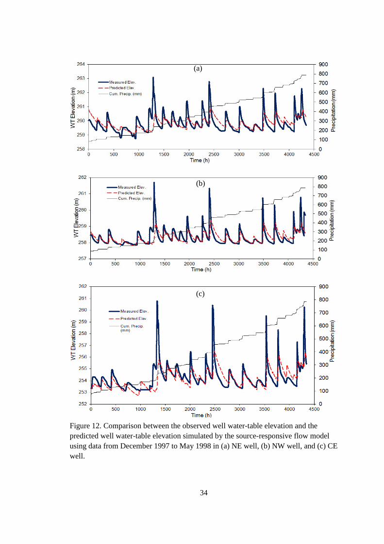
Figure 12. Comparison between the observed well water-table elevation and the predicted well water-table elevation simulated by the source-responsive flow model using data from December 1997 to May 1998 in (a) NE well, (b) NW well, and (c) CE well.
(a)
(b)
(c)
34

Figure 13. Application of the source-responsive model to measured precipitation and water-table elevations at the Masser site from February 1999 to May 1999 for (a) NE well, (b) NW well, and (c) CE well.
Time (h)
Time (h)
Time (h)
Prec
ipita
tion
(mm
) Pr
ecip
itatio
n (m
m)
Prec
ipita
tion
(mm
)
(c)
(a)
(b)
35

EMR Method
The primary analysis was performed on the set of data from the NE well during
February 1998 to May 1998; this data set had few gaps or anomalies. Having used
first order polynomial for the MRC-fitted curves, 20 h as the lag time, 0.006 as the
specific yield, and 0.45 m as the water-table-fluctuation tolerance, the method
identified 12 distinct recharge episodes for the set of data. These values gave results
that showed the most reasonable hydrologic behavior with this data set. Table 7 lists
the results of this analysis for both recharge and non-recharge intervals. Figure 14
shows the series of episodes.
The RPR values shown in Table 7 were calculated using a Sy of 0.006. The
average value was 0.30, slightly higher than the average recharge-to-precipitation
ratio estimated by Risser et al. (2009) for the same site in calendar year 1999. The
δ=0.45 m worked for most of the year, except for one instance that occurred on Jan. 7,
1998 (Fig. D2, Fig. D6, and Fig. D10 of Appendix D), which was caused by a series
of intense storms. In this event, the recharge produced by the first storm was still
taking place when the next storm started, which violates the assumption of the EMR
method. By using the same δ value, the estimated ΔH value for the first portion of
the event was unreasonably large and for the second portion was negative. In order
to prevent abnormally large RPR values and negative RPR values in the EMR
analysis results, I artificially combined those storms by adjusting the δ value to 2 m
36

for the time period from 1/6/1998 to 1/10/1998 to make the program recognize the
series of storms as a single event. Since the δ value was different from what I used
for other events, I am less confident about the results estimated by using δ=2 m
(Appendix E).
Table 7. Results of the EMR analysis for the NE well.
Interval Start
Date (in 1998)
Relative Date (days since Jan. 1, 1997)
Duration (day)
Recharge (m)
Precip. (m)
RPR (-) Avg. precip
(m)
Max. precip rate
(m/day) 1-Feb 397.25 2.51 - 0.003 - - - 3-Feb 399.76 3.39 0.009 0.037 0.252 0.011 0.175 7-Feb 403.15 4.34 - 0.001 - 0.001 0.019
11-Feb 407.48 2.75 0.006 0.013 0.471 0.004 0.097 14-Feb 410.23 2.70 - 0.001 - 0.000 0.007 16-Feb 412.93 3.91 0.010 0.038 0.263 0.010 0.128 21-Feb 416.85 2.48 - 0.001 - 0.000 0.005 23-Feb 419.33 3.07 0.011 0.059 0.179 0.019 0.246 26-Feb 422.40 9.91 - 0.008 - 0.001 0.020 8-Mar 432.30 3.13 0.011 0.024 0.447 0.008 0.169
11-Mar 435.43 8.57 - 0.010 - 0.001 0.036 20-Mar 444.00 2.90 0.012 0.028 0.441 0.010 0.155 22-Mar 446.90 9.04 - 0.004 - 0.001 0.012 31-Mar 455.94 2.74 0.006 0.019 0.297 0.007 0.274 3-Apr 458.68 4.91 - 0.000 - 0.000 0.005 8-Apr 463.59 3.04 0.012 0.057 0.220 0.018 0.236
11-Apr 466.63 6.83 - 0.006 - 0.001 0.043 18-Apr 473.46 3.11 0.013 0.050 0.258 0.016 0.181 21-Apr 476.58 4.49 - 0.000 - 0.000 0.000 26-Apr 481.07 2.66 0.005 0.023 0.229 0.008 0.079 28-Apr 483.73 5.95 - 0.014 - 0.002 0.048 4-May 489.69 2.92 0.013 0.038 0.343 0.013 0.298 7-May 492.60 0.06 - 0.000 - 0.020 0.065
37

The EMR Matlab scripts were utilized with well water-level data and
precipitation data for the entire 1997-to-1998 water year in the three adjacent
observation-wells, with some revision for overlapping events. The plots, which
show distinct behaviors between wells for the same recharge event, are presented in
Appendix D. The tabulated output results of the EMR analysis are given in
Appendix E.
Figure 14. EMR analysis for the Masser site for the NE well data from February 1998 to May 1998, of (a) H(t) data and (b) calculated dH/dt vs. time.
The ground water level in the NE well was 1.38 m higher than in the NW well,
on average, and was 5.48 m higher than in the CE well. The average ground water
level in the NW well was 4.10 m higher than in the CE well. The recharge events
lasted longer in the NE well than in the CE and NW wells. Events lasted 0.30 days
(a)
(b)
38

longer in the NE well than in the CE well on average, and lasted 0.27 days longer than
in the NW well on average. The average recharge-event durations of the CE and
NW wells were about the same, approximately 2.60 days. Comparing the recharge
start times for the same event, the CE well responded approximately 0.1 days later
than the NE and NW wells on average, and the NE well responded a little earlier than
the NW well with only 0.04 days difference on average. The average recharge
amount for each event was found to be slightly greater in the CE well than in the NE
by a factor of 1.31, and 1.79 times greater in the CE well than in the NW well. The
recharge was greater in the NE well than in the NW well by a factor of 1.26.
The average precipitation amount detected by the EMR script in different
wells for the same event was about the same. Slight differences may have been
caused by the varying durations and start times of events determined for each well by
the EMR method. The maximum rainfall intensities of the three wells estimated by
the EMR method were about the same, about 0.15 m/day on average (6.3 mm/h).
The maximum rainfall intensity detected by the method was 17.46 mm/h for the event
occurred on June 26, 1998. This value is reliable since the maximum half-hour
precipitation amount on the same day was 9.7 mm in the original precipitation record,
which is slightly greater than the EMR calculated value.
When comparing the RPR values between wells, the results for the whole year
results were separated into three parts based on the local temperature variations (Fig.
15). Figure 15 used data collected from the observation station in Fort Indiantown
39

Gap, which is about 25 km north of the Masser Site. The average daily temperatures
in November 1997, December 1997, and January 1998 were as low as the dew point.
This period was named the “cold period”. The average RPR for the cold period was
0.62. The RPR values in the spring (February to April) period were relatively small,
with an average value of 0.34 for all the three months. The RPR values were even
smaller during summer (defined as when the average daily temperatures were above
22 Celsius) with an average value of 0.27. The average RPR values for all the wells
seem reasonable when compared with previous estimations by Risser et al. (2009) and
show significant seasonal variations (Table 8). While comparing the seasonal
variations between wells, the CE well was found to have larger RPR values during the
entire year.
Figure 15. The average temperature curve for the water year from1997-98 at Fort Indiantown Gap (temperature records were searched from http://i.wund.com).
Table 8. Comparison of RPRs for different periods between the three observation wells.
Period NE Well NW Well CE Well Winter (Nov.-Jan.) 0.671 0.491 0.696 Spring (Feb.-Apr.) 0.306 0.251 0.460 Summer (May-Sep.) 0.254 0.179 0.390 Whole year (97-98) 0.442 0.344 0.535
40

DISCUSSION
Effects of Geological Factors
The sensitivity analysis for the source-responsive flow model showed that a
Mlim value of approximately 50 m-1 would work best at the Masser site in combination
with a reasonable qcap value. This means that the value of the total internal facial
area of macropores (the preferential flow paths) within the unsaturated-medium
divided by the volume of the medium should be approximately 50 m-1. This value is
much smaller than the previous value hypothesized for this site, Mlim = 4000 m-1
(Nimmo, 2010). Considering the fractured sandstone bedrock under the thin
overburden soil of the site (Fig. 3), we can suppose that the fractures form the
macropores and paths for the flux. If we assume that the fractures are more or less
planar, then the surface area for both sides of the fracture would vary from 2 m-1 to
2.82 m-1 in a characteristic volume. According to the elevations and depths of the
observation wells (Fig. 16) and the fracture analysis for the study area (Fig. 3), we can
find that the ground water-table elevation changes took place at approximately eight
to fifteen meters depth below the land surface, where the average fracture frequency is
22.875 m-1 (moderately fractured zone). If we use the fracture frequency multiplied
by the surface area of the fracture, the M value for this moderately fractured zone
should be approximately 45.75 m-1 to 64.5 m-1. This calculated range of M matches
41

the sensitivity analysis results of the source-responsive flow model very well. The
M = 50 m-1 is assumed to represent an average value that is relatively constant over
the lateral distance of the well installations.
Figure 16. Cross-section of the observation wells and core for the Masser site.
Geological factors may also account for the different behaviors between the
CE well and the NE and the NW wells indicated by the well water-table elevation vs.
time graph (Fig. 5). The CE well responded earlier than the other two wells with a
smaller initial water-table rise when the season shifted from the dry-period to the wet-
period (on November 4, 1997). The CE well also had a consistently lower water
elevation. The explanation can most likely be found in the interval-packer-testing
results (Table 2). The hydraulic conductivity for the CE well was 16.7 m/day at 35
Elev
atio
n ab
ove
sea
leve
l
42

to 38 meters depth, which is much higher compared with the hydraulic conductivity
values measured from all wells in other depth intervals. The abnormally high
hydraulic conductivity may indicate that a regional fracture zone intersects the CE
well within that depth interval, below the termination depths of the other wells. The
EMR results also shows that the CE well tends to get more recharge and have larger
RPR values for each episode than the other two wells, on average, while the water-
table elevation of the CE well was lower than the other two well. My hypothesis is
that the fracture zone located at the 35 to 38 meter interval of the CE well allows the
ground water to drain faster, which means the τ value for the CE well would be
smaller (consistent with the optimized results in Table 5) and the slope of the
recession curve would be steeper. With a steeper recession curve, the ΔH for each
recharge episode in the CE well would be larger than in the other two shallower wells
(Fig. 17), which means that a greater recharge amount would be calculated.
Figure 17. A sample hydrograph illustrates how MRC curve slope affects the ΔH value. The dashed curve has smaller τ value.
Wel
l lev
el
ΔH
43

Seasonal and Episodic Variations
Both the EMR method and the source-responsive flow model are sensitive to
the precipitation events and the seasonal weather patterns according to the above
results. The annual average temperature plot for the region (Fig. 15) shows
significant seasonal changes. Cold weather that reached the freezing point started
from November 1997 and continued to January 1998. There were several periods
that had an average daily temperature below the freezing point in December 1997 and
January 1998. Since precipitation in the form of snow or ice cannot transport
through the preferential flow paths until the snow melts, the well water-level response
may take a longer time during cold weather. The recharge-to-precipitation ratio also
shows significant seasonal variations (Table 8). The RPR values during summer
were much smaller than those during winter, which may be related to the variable air
or soil temperature, the rainfall intensity, the evapotranspiration, and the vegetation.
For instance, a plot of RPR vs. maximum rainfall intensity shows that the greater the
maximum rainfall intensity, the smaller the RPR value (Fig. 18). The RPR vs.
average rainfall intensity plot shows the same trend (Fig. 19). One hypothesis for
this phenomenon is that a large portion of the precipitation during a heavy rainfall
may go to runoff instead of producing recharge, which makes the RPR value smaller.
44

Figure 18. Plots of RPR vs. maximum rainfall intensity.
Figure 19. Plots of RPR vs. average rainfall intensity.
The seasonal changes also affect the parameters of the source-responsive flow
model. Figure 5 indicated there were two different base levels for the wet season
and the dry season over one water-year. While comparing the τ and H0 values
calculated with the MRC fitted curve for different periods, the wet season has a higher
y = 0.112x-0.577
R² = 0.4326
0
0.2
0.4
0.6
0.8
1
1.2
1.4
0 0.1 0.2 0.3 0.4 0.5
RPR
Maximum Rainfall Intensity (m/d)
RPR
Power (RPR)
y = 0.0143x-0.675
R² = 0.4747
0
0.2
0.4
0.6
0.8
1
1.2
1.4
0 0.005 0.01 0.015 0.02 0.025
RPR
Average Rainfall Intensity (m/d)
RPR
Power (RPR)
45

base level and water levels decline faster than during the dry season (Table 5). The
base-level-differences between the two periods can range from three meters in the CE
well to about ten meters in the NE and the NW wells. One possible explanation for
these phenomena is that the f(t) value is greater during the wet season, which makes it
easier for the infiltrated water to move through the vadose zone and contributes to the
ground water-table elevation rise. On the other hand, the strong evapotranspiration
during the summer and the little precipitation during the fall let the subsurface layers
dry out, which may result in minimal recharge and a lower base level.
The sensitivity analysis for Mlim and qcap indicated that the maximum
precipitation rate that could be absorbed from the land surface by preferential flow
was greatest during December to the following May (Table 6). The qcap value ranges
from 10 mm/h to 40 mm/h according to the sensitivity analysis results for the entire
water year 1997-98. From the definition of qcap (equation [17]), all the preferential
flow paths would be available when the precipitation rate is greater than the qcap value
for a specific period. For instance, the qcap value of the wet season (11/16/97-
5/15/98) was determined to be 40 mm/h while the greatest observed precipitation
intensity was 15.75 mm/h in the same period. This indicates that approximately
40% of the preferential flow paths are effectively open for input flux during that
period. The greatest observed precipitation intensity in the water year 1997-98 was
41.15 mm/h which occurred on June 23, 1998, which indicates that all the preferential
flow paths were available compared with the qcap value of 30 mm/h determined for
46

that time. A lower qcap value implies that a given storm is more likely to reach its
maximum, which means that additional rainfall intensity does not go into preferential
flow because the preferential flow paths are already flowing at their maximum
capacity. For example, a bigger proportion of the rain goes to surface runoff and
therefore less goes into recharge during summer. The source-responsive flow model
is very sensitive to the precipitation, and it worked better for the period with frequent
or regular precipitation and recharge events (wet season) than during the period with
few precipitation and recharge episodes (dry season).
Sources of Uncertainty
As a relatively new ground water recharge research approach, the EMR
method performs well for the Masser site. Errors may come from shortcomings of
the original data, subjective judgment on parameters, and the scripts. Errors may
occur when there is a gap in the data or when recharge events overlap. To avoid
these errors, I deleted the data periods where there were no water-elevation
measurements available and adjusted the width of the tolerance band to combine
overlapping events (Appendix E). This artificial revision can avoid abnormal large
RPR values or negative RPR values in the EMR analysis results. However, it may
cause underestimation of the recharge amount and there is less confidence in the
results since the criteria have been artificially changed. Several parameters were
47

initially assigned values using subjective judgment based on evaluation of the data
set, including the lag time, the specific yield, and the storm recovery time. These
parameters were adjusted several times when they were utilized in the EMR and
source-responsive model to produce the most reasonable results for the site.
One important step in both the EMR study and the source-responsive flow
model was to determine the value of the specific yield. According to a previous
study conducted by Risser et al. (2009), the average RPR for the Masser site in 1999
was 0.20, which indicated a small specific yield for the site. The value used in this
study may have still been larger than the actual value.
The lag time links the recharge episodes to the precipitation events.
Generally speaking, the lag time should vary as it is influenced by the depth of the
ground water table, the rainfall intensity, and the unsaturated-zone material. The use
of a single value of lag time may result in the inclusion of less precipitation for a
recharge episode. For instance, the start time of a recharge period that is determined
by a constant lag time is sometimes located at a time without any observed
precipitation.
The storm recovery time determines which part of the data will be used to
calculate the MRC-fitted curve. A larger storm recovery time will result in less data
being selected for the MRC estimation while a smaller storm recovery time will leave
too much data being selected for the MRC estimation; even the recharge period may
be included.
48

Overshoot in the well water-level measurements happened in the wet season
when frequent, large precipitation events occurred. The peaks of the water-level
hydrograph measured in the observation wells were sharp, and the well water level
dropped rapidly in these overshoot situations. This phenomenon is likely caused by
air entrapment as recharging water approaches the saturated zone. The source-
responsive flow model does not reflect the entrapped air that would cause overshoot.
The predicted water-table fluctuation curves underestimated many of the sharpest
hydrograph peaks (Fig. 12), which made the RMSE large, but probably resulted in
more accurate reflection of actual recharge.
When comparing the RMSE of the simulated curves for the wet seasons in the
water years 1997-98 and 1998-99, the RMSE values were somewhat smaller in 1998-
99 wet season. This is surprising since the simulated curves for the 1998-99 wet
season do not match the observed curves as well as for the water year 1997-98. One
possible reason to explain this abnormal result is that the cumulative precipitation in
the water year 1998-99 was less (Fig. 20), the infiltration rate was smaller than in the
water year 1997-98 on average, and there were fewer overshoot events in the 1998-99
wet season (Fig. 20). Taking the overshoot phenomenon (which made the measured
well water level higher than the predicted ground water level) into account, the
source-responsive flow model can provide reliable predictions and can reflect the real
water-table recharge characteristics.
49

Figure 20. The cumulative precipitation for the water year 1997-98 and 1998-99 (data provided by Dr. Gordon J. Folmar, USDA-ARS).
50

CONCLUSIONS
The Episodic Master Recession method used in this study delineated recharge
episodes by using the well water-level measurements over an entire water year and
provided an automated method to analyze the relationships between the precipitation
and the ground water recharge. The source-responsive flow model was a convenient
method to study the ground water recharge processes and was able to provide a
reliable approach to predict water-table response and recharge over many months and
multiple recharge/precipitation events based on the precipitation data. It was capable
of predicting the water-table fluctuations, both for the case where parameters were
optimized for a particular data set and when those optimized parameters were applied
to a new data set (with precipitation and well water level measured for a different time
period at the same site). In other words, the source-responsive flow model appeared
to be robust, particularly for periods with significant recharge during the wet season.
Moreover, it gave reasonable estimations of hydraulic characteristics that showed
strong relationships with the site geology. The EMR method and the source-
responsive flow model also provided results that showed the different ground water
recharge and recession characteristics between the CE well and the NE and the NW
wells, reflecting the actual fracture frequency data and the hydraulic conductivity
measurements for the different well depths. Based on the results from both methods,
the ground water recharge showed strong seasonal variations. 51

An additional advantage of both methods is that they provided a systematic
correction for overshoot and overestimation in well water-level rise. More accurate
determination of the specific yield value for the Masser site would have helped to
make the ground water recharge estimate more accurate. Also, the physical basis for
the abrupt transition in the ground water-table elevation between the dry season and
the wet season needs to be determined.
52
REFERENCES CITED
Wyrick, G. G. and Borchers, J. W., 1981, Hydrologic effects of stressed relief fracturing in an Appalachian Valley: U.S. Geological Survey, Water Supply Paper, 2117, U.S. Government Printing Office, Washington DC, p. 55.
Gburek, W.J., Urban, B.J., and Schnabel, R.R., 1986, ‘Nitrate contamination of ground
water in an upland Pennsylvania watershed’, in Proceedings of Agricultural Impacts on Ground Water: National Water Well Association, Dublin, Ohio, p. 352-380.
Gburek, W.J. and Folmar, G.J., 1999, A ground water recharge field study: site
characterization and initial results: Hydrological Processes: v. 13, p. 2813-2831. Burton, W.C., Plummer, L.N., Busenberg, E., Lindsey, B.D., and Gburek, W. J., 2002,
Influence of fracture anisotropy on ground water ages and chemistry, Valley and Ridge Province, Pennsylvania: Ground Water, v. 40, no. 3, May to June 2002, p.242-257.
Healy, C.S. and Cook, P.G., 2002, Using ground water levels to estimate recharge:
Hydrogeology Journal, v. 10, no. 1, p. 91-109. Heppner, C. S. and Nimmo, J. R., 2005, A computer program for predicting recharge
with a master recession curve: U.S. Geological Survey, Scientific Investigations Report 2005-5172.
Niu, Jianzhi and Yu, Xinxiao, 2005, Preferential flow and its scientific significance:
Science of Soil and Water Conservation. v. 3, no. 3, p.110-116. Heppner, C. S., Nimmo, J. R., Folmar G. J., Gburek, W. J., Risser, D. W., 2007,
Multiple-methods investigation of recharge at a humid-region fractured rock site, Pennsylvania, USA: Hydrogeology Journal, 2007, v. 15, p. 915-927.
Nimmo, J.R., 2010, Theory for source-responsive and free-surface film modeling of
unsaturated flow: Vadose Zone Journal. v. 9, p. 295-306. Reese, S. O. and Risser, D. W., 2010, Summary of groundwater-recharge estimates for
Pennsylvania: Pennsylvinia Geological Survey, 4th ser., Water Resource Report 70, p. 18.
53

Mirus, B.B. and Nimmo, J.R., 2013, Balancing practicality and hydrologic realism: A parsimonious approach for simulating rapid ground water recharge via unsaturated-zone preferential flow: Water Resources Research, v. 49, no. 3, p. 1458-1465.
Nimmo, J.R., Horowitz, C., and Mitchell, L., 2014, Discrete-storm water table
fluctuation method to estimate episodic recharge and climatic sensitivities: Ground Water, v. 52.
Weather Underground, 2014, Monthly History Weather in Fort Indiantow Gap, PA.
http://i.wund.com/auto/iphone/history/airport/KMUI/1997/9/30/MonthlyHistory.html
54
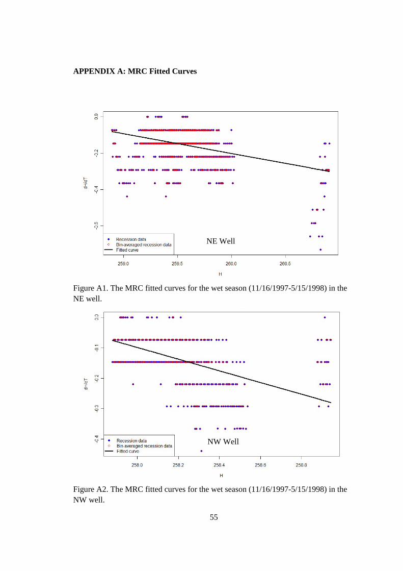
APPENDIX A: MRC Fitted Curves
Figure A1. The MRC fitted curves for the wet season (11/16/1997-5/15/1998) in the NE well.
Figure A2. The MRC fitted curves for the wet season (11/16/1997-5/15/1998) in the NW well.
NE Well
NW Well
55

Figure A3. The MRC fitted curves for the wet season (11/16/1997-5/15/1998) in the CE well.
Figure A4. The MRC fitted curves for the dry season (10/1/1997-11/15/1997 and 5/16/1998-9/30/1998) in the NE well.
CE Well
NE Well
56

Figure A5. The MRC fitted curves for the dry season (10/1/1997-11/15/1997 and 5/16/1998-9/30/1998) in the NW well.
Figure A6. The MRC fitted curves for the dry season (10/1/1997-11/15/1997 and 5/16/1998-9/30/1998) in the CE well.
NW Well
CE Well
57

Figure A7. The MRC fitted curves for the whole water year (10/1/1997-9/30/1998) in the NE well.
Figure A8. The MRC fitted curves for the whole water year (10/1/1997-9/30/1998) in the NW well.
NE Well
NW Well
58

Figure A9. The MRC Fitted Curve for the Whole Water Year (10/1/1997-9/30/1998) in the CE well.
CE Well
59

APPENDIX B: Source-Responsive Model Sensitivity Analysis
Figure B1. The sensitivity analysis for the NE well in the period 10/31/1997-11/15/1997.
Figure B2. The sensitivity analysis for the NE well in the period 11/16/1997-5/15/1998.
q cap
(mm
/h)
q cap
(mm
/h)
Mlim (m-1) RMSE Scale
Mlim (m-1) RMSE Scale
60

Figure B3. The sensitivity analysis for the NE well in the period 5/16/1998-6/17/1998.
Figure B4. The sensitivity analysis for the NE well in the period 6/24/1998-9/30/1998.
q cap
(mm
/h)
q cap
(mm
/h)
Mlim (m-1) RMSE Scale
Mlim (m-1) RMSE Scale
61
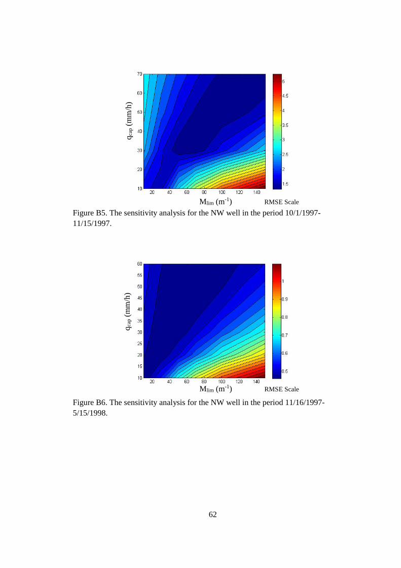
Figure B5. The sensitivity analysis for the NW well in the period 10/1/1997-11/15/1997.
Figure B6. The sensitivity analysis for the NW well in the period 11/16/1997-5/15/1998.
q cap
(mm
/h)
q cap
(mm
/h)
Mlim (m-1) RMSE Scale
Mlim (m-1) RMSE Scale
62

Figure B7. The sensitivity analysis for the NW well in the period 5/16/1998-6/17/1998.
Figure B8. The sensitivity analysis for the NW well in the period 6/24/1998-9/30/1998.
q cap
(mm
/h)
q cap
(mm
/h)
Mlim (m-1) RMSE Scale
Mlim (m-1) RMSE Scale
63
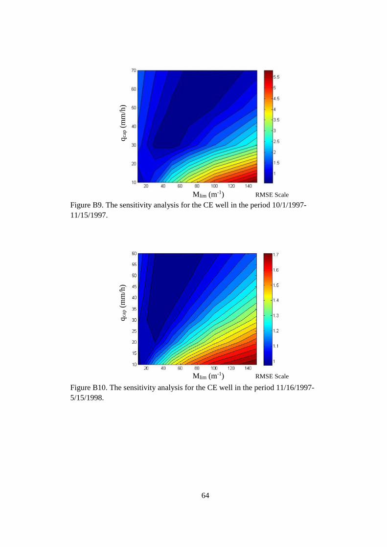
Figure B9. The sensitivity analysis for the CE well in the period 10/1/1997-11/15/1997.
Figure B10. The sensitivity analysis for the CE well in the period 11/16/1997-5/15/1998.
q cap
(mm
/h)
q cap
(mm
/h)
Mlim (m-1) RMSE Scale
Mlim (m-1) RMSE Scale
64

Figure B11. The sensitivity analysis for the CE well in the period 5/16/1998-6/25/1998.
Figure B12. The sensitivity analysis for the CE well in the period 6/26/1998-7/2/1998.
q cap
(mm
/h)
q cap
(mm
/h)
Mlim (m-1) RMSE Scale
Mlim (m-1) RMSE Scale
65

Figure B13. The sensitivity analysis for the CE well in the period 8/1/1998-9/30/1998.
q cap
(mm
/h)
Mlim (m-1) RMSE Scale
66

APPENDIX C: Source-Responsive Model Calibration Plots
Figure C1. The source-responsive model calibration for the NE well in the period 10/31/1997-11/15/1997.
Figure C2. The source-responsive model calibration for the NE well in the period 11/16/1997-5/15/1998.
020406080100
253254255256257258259260261
0 200 400 600 800 1000 1200 Pre
cipi
tatio
n (m
m)
WT
Ele
vatio
n (m
)
Time (h)
Measured Elev.Predicted Elev.Cum. Precip. (mm)
0
200
400
600
800
1000
258
259
260
261
262
263
264
0 1000 2000 3000 4000 5000
Pre
cipi
tatio
n (m
m)
WT
Ele
vatio
n (m
)
Time (h)
Measured Elev.Predicted Elev.Cum. Precip. (mm)
67

Figure C3. The source-responsive model calibration for the NE well in the period 5/16/1998-6/17/1998.
Figure C4. The source-responsive model calibration for the NE well in the period 6/24/1998-9/30/1998.
700720740760780800820840860880
256
257
258
259
260
261
0 200 400 600 800 1000
Pre
cipi
tatio
n (m
m)
WT
Ele
vatio
n (m
)
Time (h)
Measured Elev.
Predicted Elev.
Cum. Precip. (mm)
0
200
400
600
800
1000
1200
253254255256257258259260261262263
0 500 1000 1500 2000 2500
Pre
cipi
tatio
n (m
m)
WT
Ele
vatio
n (m
)
Time (h)
Measured Elev.
Predicted Elev.
Cum. Precip. (mm)
68

Figure C5. The source-responsive model calibration for the NW well in the period 10/1/1997-11/15/1997.
Figure C6. The source-responsive model calibration for the NW well in the period 11/16/1997-5/15/1998.
0
20
40
60
80
100
252
253
254
255
256
257
258
259
0 200 400 600 800 1000 1200
Pre
cipi
tatio
n (m
m)
WT
Ele
vatio
n (m
)
Time (h)
Measured Elev.
Predicted Elev.
Cum. Precip. (mm)
0100200300400500600700800900
257
258
259
260
261
262
0 1000 2000 3000 4000 5000
Pre
cipi
tatio
n (m
m)
WT
Ele
vatio
n (m
)
Time (h)
Measured Elev.Predicted Elev.Cum. Precip. (mm)
69
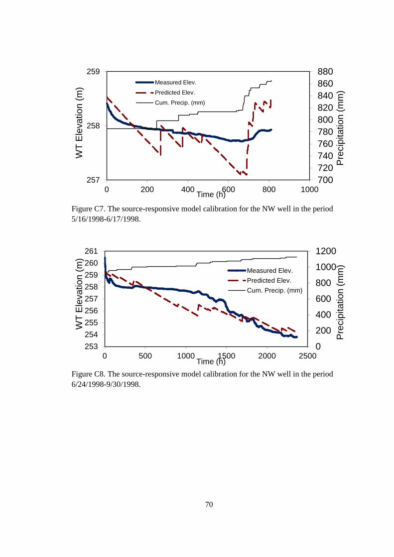
Figure C7. The source-responsive model calibration for the NW well in the period 5/16/1998-6/17/1998.
Figure C8. The source-responsive model calibration for the NW well in the period 6/24/1998-9/30/1998.
700720740760780800820840860880
257
258
259
0 200 400 600 800 1000
Pre
cipi
tatio
n (m
m)
WT
Ele
vatio
n (m
)
Time (h)
Measured Elev.
Predicted Elev.
Cum. Precip. (mm)
0
200
400
600
800
1000
1200
253254255256257258259260261
0 500 1000 1500 2000 2500
Pre
cipi
tatio
n (m
m)
WT
Ele
vatio
n (m
)
Time (h)
Measured Elev.Predicted Elev.Cum. Precip. (mm)
70

Figure C9. The source-responsive model calibration for the CE well in the period 10/1/1997-11/15/1997.
Figure C10. The source-responsive model calibration for the CE well in the period 11/16/1997-5/15/1998.
0102030405060708090
251
252
253
254
255
0 200 400 600 800 1000 1200
Pre
cipi
tatio
n (m
m)
WT
Ele
vatio
n (m
)
Time (h)
Measured Elev.
Predicted Elev.
Cum. Precip. (mm)
0100200300400500600700800900
252253254255256257258259260261262
0 1000 2000 3000 4000 5000
Pre
cipi
tatio
n (m
m)
WT
Ele
vatio
n (m
)
Time (h)
Measured Elev.Predicted Elev.Cum. Precip. (mm)
71

Figure C11. The source-responsive model calibration for the CE well in the period 5/16/1998-6/25/1998.
Figure C12. The source-responsive model calibration for the CE well in the period 6/26/1998-7/2/1998.
Figure C13. The source-responsive model calibration for the CE well in the period 8/1/1998-9/30/1998.
700
750
800
850
900
251
252
253
254
255
256
257
0 200 400 600 800 1000 1200
Pre
cipi
tatio
n (m
m)
WT
Ele
vatio
n (m
)
Time (h)
Measured Elev.Predicted Elev.Cum. Precip. (mm)
700
800
900
1000
253254255256257258259
0 50 100 150
Pre
cipi
tatio
n (m
m)
WT
Ele
vatio
n (m
)
Time (h)
Measured Elev.Predicted Elev.Cum. Precip. (mm)
0
500
1000
1500
251
252
253
254
0 500 1000 1500 2000 Pre
cipi
tatio
n (m
m)
WT
Ele
vatio
n (m
)
Time (h)
Measured Elev.Predicted Elev.Cum. Precip. (mm)
72

APPENDIX D: EMR Output Plots
Figure D1. The EMR output figures for the NE well from 10/1/1997 to 11/6/1997, of (a) H(t) data and (b) calculated dH/dt vs. time.
Figure D2. The EMR output figures for the NE well from 11/7/1997 to 2/4/1998, of (a) H(t) data and (b) calculated dH/dt vs. time.
(a)
(b)
(a)
(b)
73

Figure D3. The EMR output figures for the NE well from 2/5/1998 to 5/15/1998, of (a) H(t) data and (b) calculated dH/dt vs. time.
Figure D4. The EMR output figures for the NE well from 5/16/1998 to 9/30/1998, of (a) H(t) data and (b) calculated dH/dt vs. time.
(a)
(b)
(a)
(b)
74

Figure D5. The EMR output figures for the NW well from 10/3/1997 to 11/4/1997, of (a) H(t) data and (b) calculated dH/dt vs. time.
Figure D6. The EMR output figures for the NW well from 11/6/1997 to 2/4/1998, of (a) H(t) data and (b) calculated dH/dt vs. time.
(a)
(b)
(a)
(b)
75

Figure D7. The EMR output figures for the NW well from 2/4/1998 to 5/15/1998, of (a) H(t) data and (b) calculated dH/dt vs. time.
Figure D8. The EMR output figures for the NW well from 5/16/1998 to 9/30/1998, of (a) H(t) data and (b) calculated dH/dt vs. time.
(a)
(b)
(a)
(b)
76

Figure D9. The EMR output figures for the CE well from 10/3/1997 to 11/1/1997, of (a) H(t) data and (b) calculated dH/dt vs. time.
Figure D10. The EMR output figures for the CE well from 9/28/1997 to 2/4/1998, of (a) H(t) data and (b) calculated dH/dt vs. time.
(a)
(b)
(a)
(b)
77

Figure D11. The EMR output figures for the CE well from 2/4/1998 to 5/15/1998, of (a) H(t) data and (b) calculated dH/dt vs. time.
Figure D12. The EMR output figures for the CE well from 5/16/1998 to 6/24/1998, of (a) H(t) data and (b) calculated dH/dt vs. time.
(a)
(b)
(a)
(b)
78

Figure D13. The EMR output figures for the CE well from 6/25/1998 to 6/30/1998, of (a) H(t) data and (b) calculated dH/dt vs. time.
Figure D14. The EMR output figures for the CE well from 8/3/1998 to 9/30/1998, of (a) H(t) data and (b) calculated dH/dt vs. time.
(a)
(b)
(a)
(b)
79

APPENDIX E: EMR Output Tables
Table E1. Results of the EMR analysis for the NE well.
Time in 1997 (day)
Water level (m)
Duration (day)
Recharge (m)
Precip. (m)
RPR (-)
Avg. precip. (m/day)
Max. precip.
rate (m/day)
11/7/1997 254.09 3.965 0.034 0.026 1.303 0.007 0.091 11/14/1997 259.263 2.418 0.008 0.008 0.934 0.004 0.079 11/21/1997 259.409 2.865 0.006 0.016 0.406 0.005 0.08 11/29/1997 259.278 2.671 0.009 0.021 0.4 0.008 0.08 12/12/1997 258.827 2.965 0.007 0.01 0.704 0.003 0.076 12/24/1997 258.769 2.251 0.011 0.019 0.585 0.009 0.091 *1/7/1998 260.229 1.971 0.016 0.039 0.413 0.022 0.236 1/15/1998 259.495 2.914 0.009 0.025 0.362 0.008 0.079 1/22/1998 259.653 3.212 0.007 0.02 0.367 0.006 0.122 1/28/1998 259.674 3.275 0.006 0.005 1.245 0.001 0.014
2/3/1998 259.58 3.386 0.009 0.037 0.252 0.011 0.175 2/11/1998 259.458 2.75 0.006 0.013 0.471 0.004 0.097 2/16/1998 259.562 3.914 0.01 0.038 0.263 0.01 0.128 2/23/1998 259.656 3.068 0.011 0.059 0.179 0.019 0.246
3/8/1998 259.299 3.126 0.011 0.024 0.447 0.008 0.169 3/20/1998 259.254 2.896 0.012 0.028 0.441 0.01 0.155 3/31/1998 259.296 2.745 0.006 0.019 0.297 0.007 0.274
4/8/1998 259.345 3.042 0.012 0.057 0.22 0.018 0.236 4/18/1998 259.266 3.112 0.013 0.05 0.258 0.016 0.181 4/26/1998 259.458 2.662 0.005 0.023 0.229 0.008 0.079
5/4/1998 259.309 2.919 0.013 0.038 0.343 0.013 0.298 5/7/1998 260.305 5.963 0.01 0.055 0.191 0.009 0.098
6/13/1998 257.041 3.443 0.014 0.032 0.441 0.009 0.145 6/26/1998 259.9 1.508 0.002 0.018 0.133 0.011 0.419
7/7/1998 259.168 2.718 0.005 0.03 0.162 0.011 0.162 Average 259.143 3.030 0.010 0.028 0.442 0.009 0.152
*EMR criteria have been artificially adjusted to combine intense storms. Lack of
confidence in the results.
80
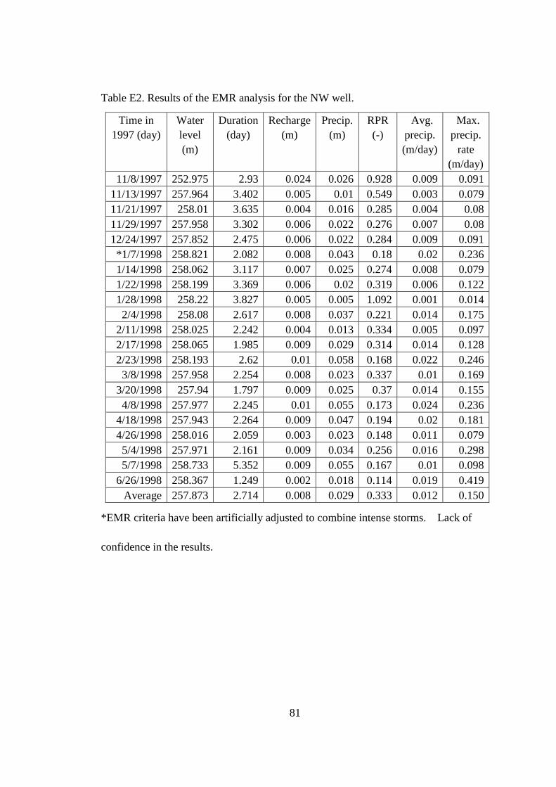
Table E2. Results of the EMR analysis for the NW well.
Time in 1997 (day)
Water level (m)
Duration (day)
Recharge (m)
Precip. (m)
RPR (-)
Avg. precip. (m/day)
Max. precip.
rate (m/day)
11/8/1997 252.975 2.93 0.024 0.026 0.928 0.009 0.091 11/13/1997 257.964 3.402 0.005 0.01 0.549 0.003 0.079 11/21/1997 258.01 3.635 0.004 0.016 0.285 0.004 0.08 11/29/1997 257.958 3.302 0.006 0.022 0.276 0.007 0.08 12/24/1997 257.852 2.475 0.006 0.022 0.284 0.009 0.091 *1/7/1998 258.821 2.082 0.008 0.043 0.18 0.02 0.236 1/14/1998 258.062 3.117 0.007 0.025 0.274 0.008 0.079 1/22/1998 258.199 3.369 0.006 0.02 0.319 0.006 0.122 1/28/1998 258.22 3.827 0.005 0.005 1.092 0.001 0.014
2/4/1998 258.08 2.617 0.008 0.037 0.221 0.014 0.175 2/11/1998 258.025 2.242 0.004 0.013 0.334 0.005 0.097 2/17/1998 258.065 1.985 0.009 0.029 0.314 0.014 0.128 2/23/1998 258.193 2.62 0.01 0.058 0.168 0.022 0.246
3/8/1998 257.958 2.254 0.008 0.023 0.337 0.01 0.169 3/20/1998 257.94 1.797 0.009 0.025 0.37 0.014 0.155
4/8/1998 257.977 2.245 0.01 0.055 0.173 0.024 0.236 4/18/1998 257.943 2.264 0.009 0.047 0.194 0.02 0.181 4/26/1998 258.016 2.059 0.003 0.023 0.148 0.011 0.079
5/4/1998 257.971 2.161 0.009 0.034 0.256 0.016 0.298 5/7/1998 258.733 5.352 0.009 0.055 0.167 0.01 0.098
6/26/1998 258.367 1.249 0.002 0.018 0.114 0.019 0.419 Average 257.873 2.714 0.008 0.029 0.333 0.012 0.150
*EMR criteria have been artificially adjusted to combine intense storms. Lack of
confidence in the results.
81
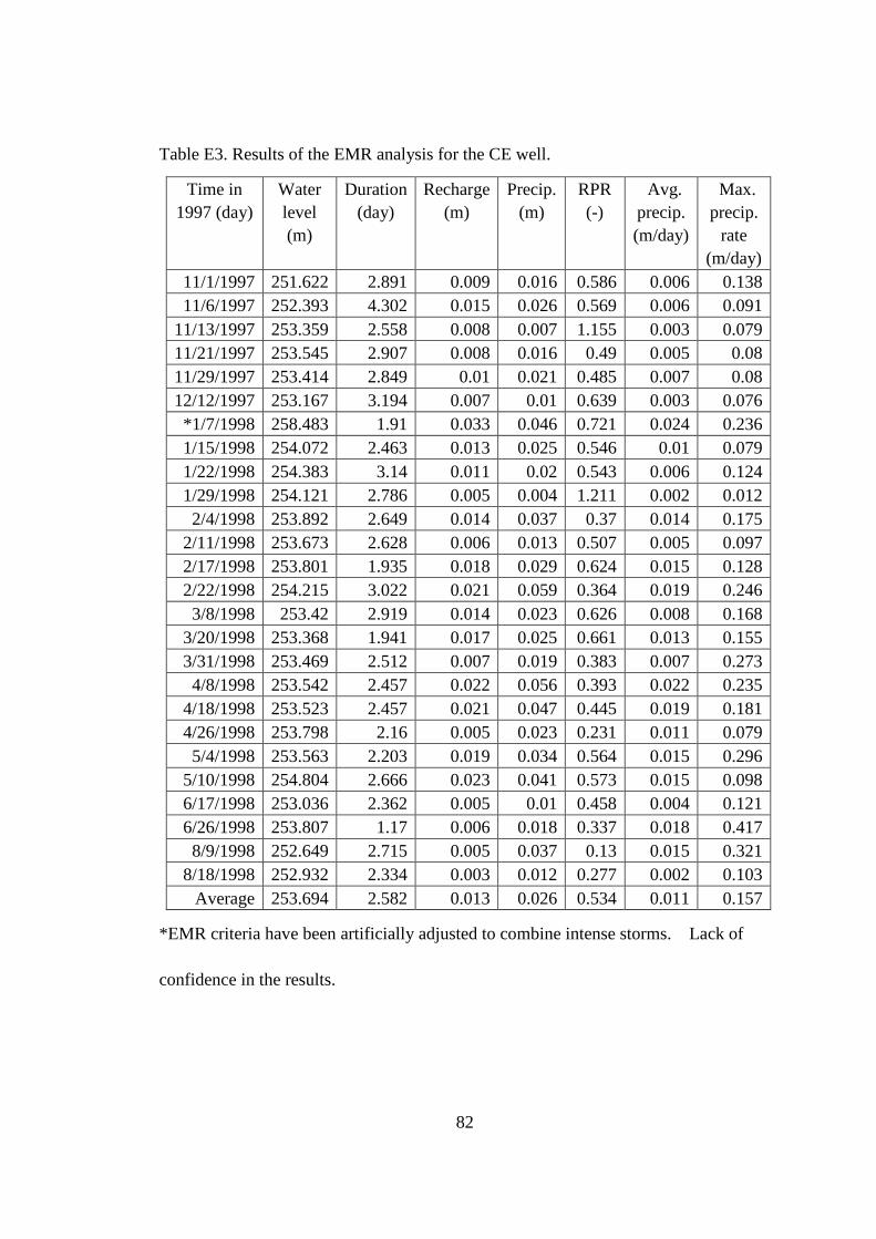
Table E3. Results of the EMR analysis for the CE well.
Time in 1997 (day)
Water level (m)
Duration (day)
Recharge (m)
Precip. (m)
RPR (-)
Avg. precip. (m/day)
Max. precip.
rate (m/day)
11/1/1997 251.622 2.891 0.009 0.016 0.586 0.006 0.138 11/6/1997 252.393 4.302 0.015 0.026 0.569 0.006 0.091
11/13/1997 253.359 2.558 0.008 0.007 1.155 0.003 0.079 11/21/1997 253.545 2.907 0.008 0.016 0.49 0.005 0.08 11/29/1997 253.414 2.849 0.01 0.021 0.485 0.007 0.08 12/12/1997 253.167 3.194 0.007 0.01 0.639 0.003 0.076 *1/7/1998 258.483 1.91 0.033 0.046 0.721 0.024 0.236 1/15/1998 254.072 2.463 0.013 0.025 0.546 0.01 0.079 1/22/1998 254.383 3.14 0.011 0.02 0.543 0.006 0.124 1/29/1998 254.121 2.786 0.005 0.004 1.211 0.002 0.012
2/4/1998 253.892 2.649 0.014 0.037 0.37 0.014 0.175 2/11/1998 253.673 2.628 0.006 0.013 0.507 0.005 0.097 2/17/1998 253.801 1.935 0.018 0.029 0.624 0.015 0.128 2/22/1998 254.215 3.022 0.021 0.059 0.364 0.019 0.246
3/8/1998 253.42 2.919 0.014 0.023 0.626 0.008 0.168 3/20/1998 253.368 1.941 0.017 0.025 0.661 0.013 0.155 3/31/1998 253.469 2.512 0.007 0.019 0.383 0.007 0.273
4/8/1998 253.542 2.457 0.022 0.056 0.393 0.022 0.235 4/18/1998 253.523 2.457 0.021 0.047 0.445 0.019 0.181 4/26/1998 253.798 2.16 0.005 0.023 0.231 0.011 0.079
5/4/1998 253.563 2.203 0.019 0.034 0.564 0.015 0.296 5/10/1998 254.804 2.666 0.023 0.041 0.573 0.015 0.098 6/17/1998 253.036 2.362 0.005 0.01 0.458 0.004 0.121 6/26/1998 253.807 1.17 0.006 0.018 0.337 0.018 0.417
8/9/1998 252.649 2.715 0.005 0.037 0.13 0.015 0.321 8/18/1998 252.932 2.334 0.003 0.012 0.277 0.002 0.103
Average 253.694 2.582 0.013 0.026 0.534 0.011 0.157
*EMR criteria have been artificially adjusted to combine intense storms. Lack of
confidence in the results.
82


![Unsaturated flow and transport through a fault embedded in ... · [2] An understanding of flow and transport in unsatu-rated fractured rock (i.e., matrix and fracture flow, and fracture-matrix](https://img.pdfslide.us/doc/110x75/5f4f2367a9b82200616d2ae7/unsaturated-flow-and-transport-through-a-fault-embedded-in-2-an-understanding.jpg)