Embed Size (px)
Citation preview

An Uncertainty-Aware Approach to OptimalConfiguration of Stream Processing Systems
Pooyan JamshidiImperial College London, UK
Email: [email protected]
Giuliano CasaleImperial College London, UK
Email: [email protected]
Abstract—Finding optimal configurations for Stream Process-ing Systems (SPS) is a challenging problem due to the largenumber of parameters that can influence their performanceand the lack of analytical models to anticipate the effect of achange. To tackle this issue, we consider tuning methods where anexperimenter is given a limited budget of experiments and needsto carefully allocate this budget to find optimal configurations.We propose in this setting Bayesian Optimization for Config-uration Optimization (BO4CO), an auto-tuning algorithm thatleverages Gaussian Processes (GPs) to iteratively capture pos-terior distributions of the configuration spaces and sequentiallydrive the experimentation. Validation based on Apache Stormdemonstrates that our approach locates optimal configurationswithin a limited experimental budget, with an improvement ofSPS performance typically of at least an order of magnitudecompared to existing configuration algorithms.
I. INTRODUCTION
We live in an increasingly instrumented world, where a largenumber of heterogeneous data sources typically provide con-tinuous data streams from live stock markets, video sources,production line status feeds, and vital body signals [12]. Yet,the research literature lacks automated methods to supportthe configuration (i.e., auto-tuning) of the underpinning SPSs.One possible explanation is that, “big data” systems suchas SPSs often combine emerging technologies that are stillpoorly understood from a performance standpoint [18], [40]and therefore difficult to holistically configure. Hence there isa critical shortage of models and tools to anticipate the effectsof changing a configuration in these systems. Examples ofconfiguration parameters for a SPS include buffer size, heapsizes, serialization/de-serialization methods, among others.
Performance differences between a well-tuned configurationand a poorly configured one can be of orders of magnitude.Typically, administrators use a mix of rules-of-thumb, trial-and-error, and heuristic methods for setting configuration pa-rameters. However, this way of testing and tuning is slow, andrequire skillful administrators with a good understanding ofthe SPS internals. Furthermore, decisions are also affected bythe nonlinear interactions between configuration parameters.
In this paper, we address the problem of finding optimalconfigurations under these requirements: (i) a configurationspace composed by multiple parameters; (ii) a limited budgetof experiments that can be allocated to test the system; (iii)experimental results affected by uncertainties due to measure-ment inaccuracies or intrinsic variability in the system process-ing times. While the literature on auto-tuning work is abundantwith existing solutions for databases, e-commerce and batchprocessing systems that address some of the above challenges
(e.g., rule-based [21], design of experiment [35], model-based[24], [18], [40], [31], search-based [38], [27], [34], [10], [1],[39] and learning-based [3]), this is the first work to considerthe problem under such constraints altogether.
In particular, we present a new auto-tuning algorithm calledBO4CO that leverages GPs [37] to continuously estimate themean and confidence interval of a response variable at yet-to-be-explored configurations. Using Bayesian optimization [30],the tuning process can account for all the available priorinformation about a system and the acquired configurationdata, and apply a variety of kernel estimators [23] to locateregions where optimal configuration may lie. To the best ofour knowledge, this is the first time that GPs are used forautomated system configuration, thus a goal of the presentwork is to introduce and apply this class of machine learningmethods into system performance tuning.
BO4CO is designed keeping in mind the limitations ofsparse sampling from the configuration space. For example,its features include: (i) sequential planning to perform ex-periments that ensure coverage of the most promising zones;(ii) memorization of past-collected samples while planningnew experiments; (iii) guarantees that optimal configurationswill be eventually discovered by the algorithm. We showexperimentally that BO4CO outperforms previous algorithmsfor configuration optimization. Our real configuration datasetsare collected for three different SPS benchmark systems,implemented with Apache Storm, and using 5 cloud clustersworth several months of experimental time.
The rest of this paper is organized as follows. Section IIdiscusses the motivations. The BO4CO algorithm is introducedin Section III and then validated in Section IV. Finally, SectionV discusses the applicability of BO4CO in practice, Section VIreviews state of the art and Section VII concludes the paper.
II. PROBLEM AND MOTIVATION
A. Problem statement
In this paper, we focus on the problem of optimal systemconfiguration defined as follows. Let Xi indicate the i-thconfiguration parameter, which takes values in a finite domainDom(Xi). In general, Xi may either indicate (i) integer vari-able such as “level of parallelism” or (ii) categorical variablesuch as “messaging frameworks” or Boolean parameter suchas “enabling timeout”. Throughout the paper, by the termoption, we mean possible values that can be assigned to aparameter. The configuration space is thus X = Dom(X1)×· · ·×Dom(Xd), which is the Cartesian product of the domains
arX
iv:1
606.
0654
3v1
[cs
.DC
] 2
1 Ju
n 20
16
Kafka Spout Splitter Bolt Counter Bolt
(sentence) (word)[paintings, 3][poems, 60][letter, 75]
Kafka Topic
Stream to Kafka
File(sentence)
(sentence)
(sen
tenc
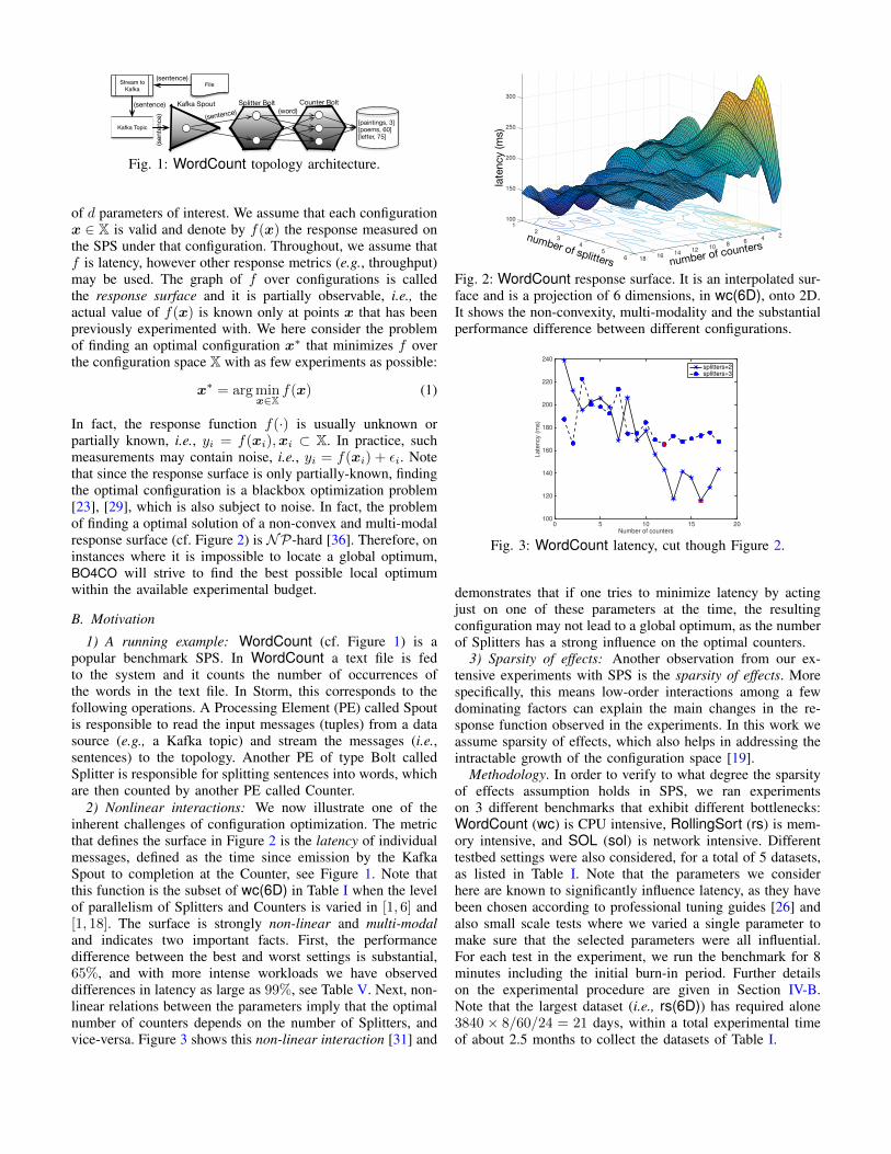
e)Fig. 1: WordCount topology architecture.
of d parameters of interest. We assume that each configurationx ∈ X is valid and denote by f(x) the response measured onthe SPS under that configuration. Throughout, we assume thatf is latency, however other response metrics (e.g., throughput)may be used. The graph of f over configurations is calledthe response surface and it is partially observable, i.e., theactual value of f(x) is known only at points x that has beenpreviously experimented with. We here consider the problemof finding an optimal configuration x∗ that minimizes f overthe configuration space X with as few experiments as possible:
x∗ = arg minx∈X
f(x) (1)
In fact, the response function f(·) is usually unknown orpartially known, i.e., yi = f(xi),xi ⊂ X. In practice, suchmeasurements may contain noise, i.e., yi = f(xi) + εi. Notethat since the response surface is only partially-known, findingthe optimal configuration is a blackbox optimization problem[23], [29], which is also subject to noise. In fact, the problemof finding a optimal solution of a non-convex and multi-modalresponse surface (cf. Figure 2) is NP-hard [36]. Therefore, oninstances where it is impossible to locate a global optimum,BO4CO will strive to find the best possible local optimumwithin the available experimental budget.
B. Motivation
1) A running example: WordCount (cf. Figure 1) is apopular benchmark SPS. In WordCount a text file is fedto the system and it counts the number of occurrences ofthe words in the text file. In Storm, this corresponds to thefollowing operations. A Processing Element (PE) called Spoutis responsible to read the input messages (tuples) from a datasource (e.g., a Kafka topic) and stream the messages (i.e.,sentences) to the topology. Another PE of type Bolt calledSplitter is responsible for splitting sentences into words, whichare then counted by another PE called Counter.
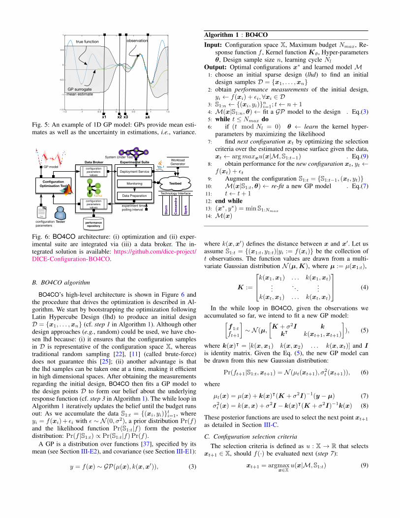
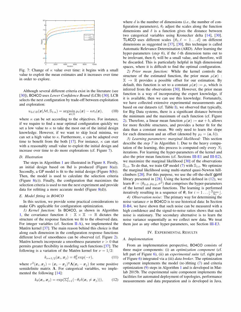
2) Nonlinear interactions: We now illustrate one of theinherent challenges of configuration optimization. The metricthat defines the surface in Figure 2 is the latency of individualmessages, defined as the time since emission by the KafkaSpout to completion at the Counter, see Figure 1. Note thatthis function is the subset of wc(6D) in Table I when the levelof parallelism of Splitters and Counters is varied in [1, 6] and[1, 18]. The surface is strongly non-linear and multi-modaland indicates two important facts. First, the performancedifference between the best and worst settings is substantial,65%, and with more intense workloads we have observeddifferences in latency as large as 99%, see Table V. Next, non-linear relations between the parameters imply that the optimalnumber of counters depends on the number of Splitters, andvice-versa. Figure 3 shows this non-linear interaction [31] and
number of countersnumber of splitters
late
ncy
(ms)
100
150
1
200
250
2
300
Cubic Interpolation Over Finer Grid
243
684 10
125 14166 18
Fig. 2: WordCount response surface. It is an interpolated sur-face and is a projection of 6 dimensions, in wc(6D), onto 2D.It shows the non-convexity, multi-modality and the substantialperformance difference between different configurations.
0 5 10 15 20Number of counters
100
120
140
160
180
200
220
240
La
ten
cy (
ms)
splitters=2splitters=3
Fig. 3: WordCount latency, cut though Figure 2.
demonstrates that if one tries to minimize latency by actingjust on one of these parameters at the time, the resultingconfiguration may not lead to a global optimum, as the numberof Splitters has a strong influence on the optimal counters.
3) Sparsity of effects: Another observation from our ex-tensive experiments with SPS is the sparsity of effects. Morespecifically, this means low-order interactions among a fewdominating factors can explain the main changes in the re-sponse function observed in the experiments. In this work weassume sparsity of effects, which also helps in addressing theintractable growth of the configuration space [19].
Methodology. In order to verify to what degree the sparsityof effects assumption holds in SPS, we ran experimentson 3 different benchmarks that exhibit different bottlenecks:WordCount (wc) is CPU intensive, RollingSort (rs) is mem-ory intensive, and SOL (sol) is network intensive. Differenttestbed settings were also considered, for a total of 5 datasets,as listed in Table I. Note that the parameters we considerhere are known to significantly influence latency, as they havebeen chosen according to professional tuning guides [26] andalso small scale tests where we varied a single parameter tomake sure that the selected parameters were all influential.For each test in the experiment, we run the benchmark for 8minutes including the initial burn-in period. Further detailson the experimental procedure are given in Section IV-B.Note that the largest dataset (i.e., rs(6D)) has required alone3840 × 8/60/24 = 21 days, within a total experimental timeof about 2.5 months to collect the datasets of Table I.

TABLE I: Sparsity of effects on 5 experiments where we have varieddifferent subsets of parameters and used different testbeds. Note thatthese are the datasets we experimentally measured on the benchmarksystems and we use them for the evaluation, more details includingthe results for 6 more experiments are in the appendix.
Topol. Parameters Main factors Merit Size Testbed
1 wc(6D)1-spouts, 2-max spout,3-spout wait, 4-splitters,5-counters, 6-netty min wait
{1, 2, 5} 0.787 2880 C1
2 sol(6D)1-spouts, 2-max spout,3-top level, 4-netty min wait,5-message size, 6-bolts
{1, 2, 3} 0.447 2866 C2
3 rs(6D)1-spouts, 2-max spout,3-sorters, 4-emit freq,5-chunk size, 6-message size
{3} 0.385 3840 C3
4 wc(3D) 1-max spout, 2-splitters,3-counters {1, 2} 0.480 756 C4
5 wc(5D)1-spouts, 2-splitters,3-counters,4-buffer-size, 5-heap
{1} 0.851 1080 C5
wc wc+rs wc+sol 2wc 2wc+rs+sol
101
102
La
ten
cy (
ms)
Fig. 4: Noisy experimental measurements. Note that + heremeans that wc is deployed in a multi-tenant environmentwith other topologies and as a result not only the latency isincreased but also the variability became greater.
Results. After collecting experimental data, we have useda common correlation-based feature selector1 implemented inWeka to rank parameter subsets according to a heuristic. Thebias of the merit function is toward subsets that contain pa-rameters that are highly correlated with the response variable.Less influential parameters are filtered because they will havelow correlation with latency, and a set with the main factorsis returned. For all of the 5 datasets, we list in Table I themain factors. The analysis results demonstrate that in all the 5experiments at most 2-3 parameters were strongly interactingwith each other, out of a maximum of 6 parameters variedsimultaneously. Therefore, the determination of the regionswhere performance is optimal will likely be controlled by suchdominant factors, even though the determination of a globaloptimum will still depends on all the parameters.
4) Measurement uncertainty: We now illustrate measure-ment variabilities, which represent an additional challenge forconfiguration optimization. As depicted in Figure 4, we took
1The most significant parameters are selected based on the following meritfunction [9], also shown in Table I:
mps =nrlp√
n+ n(n− 1)rpp, (2)
where rlp is the mean parameter-latency correlation, n is the number ofparameters, rpp is the average feature-feature inter-correlation [9, Sec 4.4].
different samples of the latency metric over 2 hours for fivedifferent deployments of WordCount. The experiments runon a multi-node cluster on the EC2 cloud. After filtering theinitial burn-in, we computed averages and standard deviationof the latencies. Note that the configuration across all 5settings is similar, the only difference is the number of co-located topologies in the testbed. The data in boxplots illustratethat variability can be small in some settings (e.g., wc),while they can be large in some other experimental setups(e.g., 2wc+rs+sol). In traditional techniques such as designof experiments, such variability is addressed by repeatingexperiments multiple times and obtaining regression estimatesfor the system model across such repetitions. However, wehere pursue the alternative approach of relying on GP modelsto capture both mean and variance of measurements withinthe model that guides the configuration process. The theoryunderpinning this approach is discussed in the next section.
III. BO4CO: BAYESIAN OPTIMIZATION FORCONFIGURATION OPTIMIZATION
A. Bayesian Optimization with Gaussian Process prior
Bayesian optimization is a sequential design strategy thatallows us to perform global optimization of blackbox functions[30]. The main idea of this method is to treat the blackboxobjective function f(x) as a random variable with a given priordistribution, and then perform optimization on the posteriordistribution of f(x) given experimental data. In this work,GPs are used to model this blackbox objective function at eachpoint x ∈ X. That is, let S1:t be the experimental data collectedin the first t iterations and let xt+1 be a candidate configurationthat we may select to run the next experiment. Then BO4COassesses the probability that this new experiment could findan optimal configuration using the posterior distribution:
Pr(ft+1|S1:t,xt+1) ∼ N (µt(xt+1), σ2t (xt+1)),
where µt(xt+1) and σ2t (xt+1) are suitable estimators of the
mean and standard deviation of a normal distribution that isused to model this posterior. The main motivation behind thechoice of GPs as prior here is that it offers a framework inwhich reasoning can be not only based on mean estimatesbut also the variance, providing more informative decisionmakings. The other reason is that all the computations in thisframework are based on linear algebra.
Figure 5 illustrates the GP-based Bayesian optimizationusing a 1-dimensional response surface. The curve in blue isthe unknown true posterior distribution, whereas the mean isshown in green and the 95% confidence interval at each pointin the shaded area. Stars indicate measurements carried out inthe past and recorded in S1:t (i.e., observations). Configurationcorresponds to x1 has a large confidence interval due to lack ofobservations in its neighborhood. Conversely, x4 has a narrowconfidence since neighboring configurations have been exper-imented with. The confidence interval in the neighborhood ofx2 and x3 is not high and correctly our approach does notdecide to explore these zones. The next configuration xt+1,indicated by a small circle right to the x4, is selected basedon a criterion that will be defined later.
-1.5 -1 -0.5 0 0.5 1 1.5-1.5
-1
-0.5
0
0.5
1
x1 x2 x3 x4
true function
GP surrogate mean estimate
observation
Fig. 5: An example of 1D GP model: GPs provide mean esti-mates as well as the uncertainty in estimations, i.e., variance.
Configuration Optimisation Tool
performance repository
Monitoring
Deployment Service
Data Preparation
configuration parameters
values
configuration parameters
values
Experimental Suite
Testbed
Doc
Data Broker
Tester
experiment timepolling interval
configurationparameters
GP model
Kafka
System Under TestWorkloadGenerator
Technology Interface
Stor
m
Cas
sand
ra
Spar
k
Fig. 6: BO4CO architecture: (i) optimization and (ii) exper-imental suite are integrated via (iii) a data broker. The in-tegrated solution is available: https://github.com/dice-project/DICE-Configuration-BO4CO.
B. BO4CO algorithm
BO4CO’s high-level architecture is shown in Figure 6 andthe procedure that drives the optimization is described in Al-gorithm. We start by bootstrapping the optimization followingLatin Hypercube Design (lhd) to produce an initial designD = {x1, . . . ,xn} (cf. step 1 in Algorithm 1). Although otherdesign approaches (e.g., random) could be used, we have cho-sen lhd because: (i) it ensures that the configuration samplesin D is representative of the configuration space X, whereastraditional random sampling [22], [11] (called brute-force)does not guarantee this [25]; (ii) another advantage is thatthe lhd samples can be taken one at a time, making it efficientin high dimensional spaces. After obtaining the measurementsregarding the initial design, BO4CO then fits a GP model tothe design points D to form our belief about the underlyingresponse function (cf. step 3 in Algorithm 1). The while loop inAlgorithm 1 iteratively updates the belief until the budget runsout: As we accumulate the data S1:t = {(xi, yi)}ti=1, whereyi = f(xi) + εi with ε ∼ N (0, σ2), a prior distribution Pr(f)and the likelihood function Pr(S1:t|f) form the posteriordistribution: Pr(f |S1:t) ∝ Pr(S1:t|f) Pr(f).
A GP is a distribution over functions [37], specified by itsmean (see Section III-E2), and covariance (see Section III-E1):
y = f(x) ∼ GP(µ(x), k(x,x′)), (3)
Algorithm 1 : BO4COInput: Configuration space X, Maximum budget Nmax, Re-
sponse function f , Kernel function Kθ, Hyper-parametersθ, Design sample size n, learning cycle Nl
Output: Optimal configurations x∗ and learned model M1: choose an initial sparse design (lhd) to find an initial
design samples D = {x1, . . . ,xn}2: obtain performance measurements of the initial design,yi ← f(xi) + εi,∀xi ∈ D
3: S1:n ← {(xi, yi)}ni=1; t← n+ 14: M(x|S1:n,θ)← fit a GP model to the design . Eq.(3)5: while t ≤ Nmax do6: if (t mod Nl = 0) θ ← learn the kernel hyper-
parameters by maximizing the likelihood7: find next configuration xt by optimizing the selection
criteria over the estimated response surface given the data,xt ← argmaxxu(x|M,S1:t−1) . Eq.(9)
8: obtain performance for the new configuration xt, yt ←f(xt) + εt
9: Augment the configuration S1:t = {S1:t−1, (xt, yt)}10: M(x|S1:t,θ)← re-fit a new GP model . Eq.(7)11: t← t+ 112: end while13: (x∗, y∗) = minS1:Nmax
14: M(x)
where k(x,x′) defines the distance between x and x′. Let usassume S1:t = {(x1:t, y1:t)|yi := f(xi)} be the collection oft observations. The function values are drawn from a multi-variate Gaussian distribution N (µ,K), where µ := µ(x1:t),
K :=
k(x1,x1) . . . k(x1,xt)...
. . ....
k(xt,x1) . . . k(xt,xt)
(4)
In the while loop in BO4CO, given the observations weaccumulated so far, we intend to fit a new GP model:[
f1:t
ft+1
]∼ N (µ,
[K + σ2I kkᵀ k(xt+1,xt+1)
]), (5)
where k(x)ᵀ = [k(x,x1) k(x,x2) . . . k(x,xt)] and Iis identity matrix. Given the Eq. (5), the new GP model canbe drawn from this new Gaussian distribution:
Pr(ft+1|S1:t,xt+1) = N (µt(xt+1), σ2t (xt+1)), (6)
where
µt(x) = µ(x) + k(x)ᵀ(K + σ2I)−1(y − µ) (7)σ2t (x) = k(x,x) + σ2I − k(x)ᵀ(K + σ2I)−1k(x) (8)
These posterior functions are used to select the next point xt+1
as detailed in Section III-C.
C. Configuration selection criteriaThe selection criteria is defined as u : X → R that selects
xt+1 ∈ X, should f(·) be evaluated next (step 7):
xt+1 = argmaxx∈X
u(x|M,S1:t) (9)
0 2000 4000 6000 8000 10000Iteration
4
4.5
5
5.5
6
6.5
7
7.5
8
8.5
Ka
pp
a
ǫ=1ǫ=0.1ǫ=0.01
Fig. 7: Change of κ value over time: it begins with a smallvalue to exploit the mean estimates and it increases over timein order to explore.
Although several different criteria exist in the literature (see[30]), BO4CO uses Lower Confidence Bound (LCB) [30]. LCBselects the next configuration by trade-off between exploitationand exploration:
uLCB(x|M,S1:n) = argminx∈X
µt(x)− κσt(x), (10)
where κ can be set according to the objectives. For instance,if we require to find a near optimal configuration quickly weset a low value to κ to take the most out of the initial designknowledge. However, if we want to skip local minima, wecan set a high value to κ. Furthermore, κ can be adapted overtime to benefit from the both [17]. For instance, κ can startwith a reasonably small value to exploit the initial design andincrease over time to do more explorations (cf. Figure 7).
D. IllustrationThe steps in Algorithm 1 are illustrated in Figure 8. Firstly,
an initial design based on lhd is produced (Figure 8(a)).Secondly, a GP model is fit to the initial design (Figure 8(b)).Then, the model is used to calculate the selection criteria(Figure 8(c)). Finally, the configuration that maximizes theselection criteria is used to run the next experiment and providedata for refitting a more accurate model (Figure 8(d)).
E. Model fitting in BO4COIn this section, we provide some practical considerations to
make GPs applicable for configuration optimization.1) Kernel function: In BO4CO, as shown in Algorithm
1, the covariance function k : X × X → R dictates thestructure of the response function we fit to the observed data.For integer variables (cf. Section II-A), we implemented theMatern kernel [37]. The main reason behind this choice is thatalong each dimension in the configuration response functionsdifferent level of smoothness can be observed (cf. Figure 2).Matern kernels incorporate a smoothness parameter ν > 0 thatpermits greater flexibility in modeling such functions [37]. Thefollowing is a variation of the Matern kernel for ν = 1/2:
kν=1/2(xi,xj) = θ20 exp(−r), (11)
where r2(xi,xj) = (xi − xj)ᵀΛ(xi − xj) for some positivesemidefinite matrix Λ. For categorical variables, we imple-mented the following [14]:
kθ(xi,xj) = exp(Σd`=1(−θ`δ(xi 6= xj))), (12)
where d is the number of dimensions (i.e., the number of con-figuration parameters), θ` adjust the scales along the functiondimensions and δ is a function gives the distance betweentwo categorical variables using Kronecker delta [14], [30].TL4CO uses different scales {θ`, ` = 1 . . . d} on differentdimensions as suggested in [37], [30], this technique is calledAutomatic Relevance Determination (ARD). After learning thehyper-parameters (step 6), if the `-th dimension turns out tobe irrelevant, then θ` will be a small value, and therefore, willbe discarded. This is particularly helpful in high dimensionalspaces, where it is difficult to find the optimal configuration.
2) Prior mean function: While the kernel controls thestructure of the estimated function, the prior mean µ(x) :X → R provides a possible offset for our estimation. Bydefault, this function is set to a constant µ(x) := µ, which isinferred from the observations [30]. However, the prior meanfunction is a way of incorporating the expert knowledge, ifit is available, then we can use this knowledge. Fortunately,we have collected extensive experimental measurements andbased on our datasets (cf. Table I), we observed that typically,for Big Data systems, there is a significant distance betweenthe minimum and the maximum of each function (cf. Figure2). Therefore, a linear mean function µ(x) := ax+ b, allowsfor more flexible structures, and provides a better fit for thedata than a constant mean. We only need to learn the slopefor each dimension and an offset (denoted by µ` = (a, b)).
3) Learning parameters: marginal likelihood: This sectiondescribe the step 7 in Algorithm 1. Due to the heavy compu-tation of the learning, this process is computed only every Nliterations. For learning the hyper-parameters of the kernel andalso the prior mean functions (cf. Sections III-E1 and III-E2),we maximize the marginal likelihood [30] of the observationsS1:t. To do that, we train GP model (7) with S1:t. We optimizethe marginal likelihood using multi-started quasi-Newton hill-climbers [28]. For this purpose, we use the off-the-shelf gpmllibrary presented in [28]. Using the kernel defined in (12), welearn θ := (θ0:d, µ0:d, σ
2) that comprises the hyper-parametersof the kernel and mean functions. The learning is performediteratively resulting in a sequence of θi for i = 1 . . . bNmax
N`c.
4) Observation noise: The primary way for determining thenoise variance σ in BO4CO is to use historical data: In SectionII-B4, we have shown that such noise can be measured with ahigh confidence and the signal-to-noise ratios shows that suchnoise is stationary. The secondary alternative is to learn thenoise variance sequentially as we collect new data. We treatthem just as any other hyper-parameters, see Section III-E3.
IV. EXPERIMENTAL RESULTS
A. Implementation
From an implementation perspective, BO4CO consists ofthree major components: (i) an optimization component (cf.left part of Figure 6), (ii) an experimental suite (cf. right partof Figure 6) integrated via a (iii) data broker. The optimizationcomponent implements the model (re-)fitting (7) and criteriaoptimization (9) steps in Algorithm 1 and is developed in Mat-lab 2015b. The experimental suite component implements thefacilities for automated deployment of topologies, performancemeasurements and data preparation and is developed in Java.

-1.5 -1 -0.5 0 0.5 1 1.5-0.8
-0.6
-0.4
-0.2
0
0.2
0.4
0.6
0.8
-1.5 -1 -0.5 0 0.5 1 1.5-0.8
-0.6
-0.4
-0.2
0
0.2
0.4
0.6
0.8
1
-1.5 -1 -0.5 0 0.5 1 1.5-0.8
-0.6
-0.4
-0.2
0
0.2
0.4
0.6
0.8
1
-1.5 -1 -0.5 0 0.5 1 1.5-0.8
-0.6
-0.4
-0.2
0
0.2
0.4
0.6
0.8
1
configuration domain
resp
onse
val
ue
(a) (b)
(c) (d)
true response function
criteria evaluation
GP fit
new selected point
new GP fit
excl
uded
regi
onFig. 8: Illustration of configuration parameter optimization: (a)initial observations; (b) a GP model fit; (c) choosing the nextpoint; (d) refitting a new GP model.
-1.5 -1 -0.5 0 0.5 1 1.5-0.8
-0.6
-0.4
-0.2
0
0.2
0.4
0.6
0.8
1
1.2true functionobservationmatern1matern3matern5matern-ard
Fig. 9: The effect of changing the kernel in estimations.
The optimization component retrieves the initial design per-formance data and determines which configuration to try nextusing the procedure explained in III-C. The suite then deploysthe topology under test on a testing cluster. The performance ofthe topology is then measured and the performance data will beused for model refitting. We have released the code and data:https://github.com/dice-project/DICE-Configuration-BO4CO.
In order to make BO4CO more practical and relevant forindustrial use, we considered several implementation enhance-ments. In order to perform efficient GP model re-fitting, weimplemented a covariance wrapper function that keeps theinternal state for caching kernels and its derivatives, and canupdate kernel function by a single element. This was particu-larly helpful for learning the hyper-parameters at runtime.
B. Experimental design1) Topologies under test and benchmark functions: In
this section, we evaluate BO4CO using 3 different Stormbenchmarks: (i) WordCount, (ii) RollingSort, (iii) SOL.RollingSort implements a common pattern in real-time dataanalysis that performs rolling counts of incoming messages.RollingSort is used by Twitter for identifying trending topics.SOL is a network intensive topology, where the incomingmessages will be routed through an inter-worker network.
WordCount and RollingSort are standard benchmarks andare widely used in the community, e.g., research papers [7]and industry scale benchmarks [13]. We have conducted allthe experiments on 5 cloud clusters and with different sets ofparameters resulted in datasets in Table I.
We also evaluate BO4CO with a number of benchmarkfunctions, where we perform a synthetic experiment insideMATLAB in which a measurement is just a function eval-uation: Branin(2D), Dixon-Szego(2D), Hartmann(3D) andRosenbrock(5D). These benchmark functions are commonlyused in global optimization and configuration approaches[38], [34]. We particularly selected these because: (i) theyhave different curvature and (ii) they have multiple globalminimizers, and (iii) they are of different dimensions.
2) Baseline approaches: The performance of BO4CO iscompared with the 5 outstanding state-of-the-art approachesfor configuration optimizations: SA [8], GA [1], HILL [38],PS [34] and Drift [33]. They are of different nature anduse different search algorithms: simulated annealing, geneticalgorithm, hill climbing, pattern search and adaptive search.
3) Experimental considerations: The performance statisticsregarding each specific configuration has been collected overa window of 5 minutes (excluding the first two minutes ofburn-in and the last minute of cluster cleaning). The firsttwo minutes are excluded because the monitoring data arenot stationary, while the last minute is the time given to thetopology to fully process all messages. We then shut down thetopology, clean the cluster and move on to the next experiment.We also replicated each runs of algorithms for 30 times inorder to report the comparison results. Therefore, all the resultspresented in this paper are the mean performance over 30 runs.
4) Cluster configuration: We conducted all the experimentson 5 different multi-node clusters on three various cloud plat-forms, see A for more details. The reason behind this decisionwas twofold: (i) saving time in collecting experimental databy running topologies in parallel as some of the experimentssupposed to run for several weeks, see Section II-B3. (ii)replicating the experiment with different processing node.
C. Experimental analysisIn the following, we evaluate the performance of each
approach as a function of the number of evaluations. So foreach case, we report performance using the absolute distanceof the minimum function value from the global minimum.Since we have measured all combinations of parameters inour datasets, we can measure this distance at each iteration.
1) Benchmark functions global optimization: The resultsfor Branin in Figure 10(a) show that BO4CO outperforms theother approaches with three orders of magnitude, while thisgap is only an order of magnitude for Dixon as in Figure 10(b).This difference can be associated to the fact that Dixon surfaceis more rugged than Branin [36]. For Branin, BO4CO findsthe global minimum within the first 40 iterations, while evenSA stalls on a local minimum. The rest, including GA, HILL,PS perform similarly to each other throughout the experimentand reach a local minimum, which BO4CO finds only withinthe first 10 iterations. For Dixon, BO4CO gets close to theglobal minimum within the first 20 iterations, while the bestperformers (i.e., PS and HILL) approach to points an order of
0 20 40 60 80 100
Iteration
10-4
10-3
10-2
10-1
100
101
102
Absolu
te E
rror
BO4CO
SA
GA
HILL
PS
Drift
0 20 40 60 80 100Iteration
10-2
10-1
100
101
Abso
lute
Erro
r
BO4COSAGAHILLPSDrift
(a) Branin(2D) (b) Dixon(2D)
Fig. 10: Branin(2D), Dixon(2D) test function optimization.
x∗
1 x∗
2 x∗
3
0
0.1
0.2
0.3
BO
4C
O
x∗
1 x∗
2 x∗
3
0
2
4
SA
x∗
1 x∗
2 x∗
3
02468
GA
x∗
1 x∗
2 x∗
3
0
1
2
HIL
L
x∗
1 x∗
2 x∗
3
0.5
1
1.5
PS
x∗
1 x∗
2 x∗
3
0
5
10
15
Drift
Fig. 11: Distance to the three Branin’s minimizers.
magnitude away comparing with BO4CO. Branin function has3 global minimizers at x∗1 = (π, 12.27), x∗2 = (π, 2.27), x∗3 =(9.42, 2.47), interestingly comparing to baselines, BO4CO getsclose to all minimizers (cf. Figure 11). Therefore, BO4COgains information on all minimizers as opposed to baselines.
The results for Hartmann in Figure 12(a) show that BO4COdecreases the absolute error quickly after 20 iterations, butonly approaches to the global minimum after 120 iterations.Neither of the baseline approaches get close to the globalminimum even after 150 iterations. The good performanceof BO4CO is also confirmed in the case of Rosenbrock, asshown in Figure 12(b). BO4CO finds the optimum in suchlarge space only after 60 iterations, while GA, HILL, PS andDrift perform poorly with an error of three orders of magnitudehigher than our approach. However, SA performs well with anorder of magnitude away from the ones found by BO4CO.
2) Storm configuration optimization: We now discuss theresults of BO4CO on the Storm datasets in Table I: SOL(6D),RollingSort(6D), WordCount(3D,5D).
The results for SOL in Figure 13(a) show that BO4COdecreases the optimality gap within the first 10 iterations anddecreases this gap until iteration 200 and does not get trappedinto a local minimum. Instead, baseline approaches like Driftand GA get trapped into a local minimum in early iterations,while HILL and PS get stuck some iterations later at 120.Among the baselines, SA performs the best and it decreasesthe optimality gap in the first 70 iterations, however, it getsstuck to a local optimum thereafter.
The results for RollingSort in Figure 13(b) are similar tothe SOL ones. BO4CO decreases the error considerably in
0 50 100 150Iteration
10-3
10-2
10-1
100
101
Abso
lute
Erro
r
BO4COSAGAHILLPSDrift
0 50 100 150 200 250Iteration
102
103
104
105
106
107
108
Abso
lute
Erro
r
BO4COSAGAHILLPSDrift
(a) Hartmann(3D) (b) Rosenbrock(5D)
Fig. 12: Hartmann(3D), Rosenbrock(5D) optimization.
0 50 100 150 200
Iteration
10-2
10-1
100
101
102
103
104
Abso
lute
Err
or
BO4CO
SA
GA
HILL
PS
Drift
0 50 100 150 200
Iteration
10-2
10-1
100
101
102
103
104
Abso
lute
Err
or
BO4CO
SA
GA
HILL
PS
Drift
(a) SOL(6D) (b) RollingSort(6D)
Fig. 13: SOL(6D), RollingSort(6D) optimization.
the first 50 iterations, while the baseline approaches, exceptSA and HILL, perform poorly in that period. However, duringiterations 100-200, the rests, except GA and Drift, find con-figuration with close performance as the ones BO4CO finds.
For WordCount (Figure 14(a,b)) the results are different.BO4CO outperforms the best baseline performer, i.e., SA, byan order of magnitude, while the others by at least two ordersof magnitude. Among the baselines, SA performs the bestfor WordCount(3D), while for WordCount(5D) dataset, HILLand PS performs better in the first 50 iterations.
Summarizing, while the results for the Storm benchmarksare consistent with the ones we observed for the benchmarkfunctions, it shows a clear gain in favor of BO4CO, with atleast an order of magnitude in the initial iterations. In eachcase, BO4CO finds a better configuration much more quicklythan baselines. As opposed to the benchmark functions, SAconsistently outperforms the rest of baseline approaches. Tohighlight this achievement, note that 50 iterations for a datasetlike SOL (6D) is only 1% of the total number of possible testsfor finding the optimum configurations and identifying suchconfigurations with a latency close to the global optimum cansave a considerable time and cost.
D. Sensitivity analysis
1) Prediction accuracy of the learned GP model: SinceBO4CO does not uniformly sample the configuration space(cf. Figure 5,8), we speculated that the GP models trainedin BO4CO are not useful for predicting the performance ofconfigurations that have not been experimented. However,when we compared the GP model on the WordCount, itwas much more accurate than the ones of polynomial re-gressions (see Figure 15). This shows a clear advantage overdesign of experiments (DoE), which normally uses first-orderand second-order polynomials. The root mean squared error

0 20 40 60 80 100
Iteration
10-3
10-2
10-1
100
101
102
103
104
Ab
so
lute
Err
or
BO4CO
SA
GA
HILL
PS
Drift
0 20 40 60 80 100
Iteration
10-2
10-1
100
101
102
103
Ab
so
lute
Err
or
BO4CO
SA
GA
HILL
PS
Drift
(a) WordCount(3D) (b) WordCount(5D)
Fig. 14: WordCount(3D,5D) configuration optimization.
BO4CO polyfit1 polyfit2 polyfit3 polyfit4 polyfit5
10-10
10-8
10-6
10-4
10-2
100
102
Absolu
te P
erc
enta
ge
Err
or
[%]
Fig. 15: Absolute percentage error of predictions made byBO4CO’s GP fit after 100 iterations vs multivariate polynomialregression models for WordCount(3D) dataset.
(RMSE) for Branin and Dixon in 16(a) clearly show that theGP models can provide accurate predictions after 20 iterations.This fast learning rate can be associated to the power ofGPs for regressions [37]. We further compared the predictionaccuracy of the GP models trained in BO4CO with severalmachine learning models (including M5Tree, RegressionTree, LWP, PRIM [37]) in Figure 16(b) and we observedthat the GP model predictions were more accurate, while theaccuracy of other models either did not improve (e.g., M5Tree)or was deteriorated (e.g., PRIM, polyfit5) due to over-fitting.
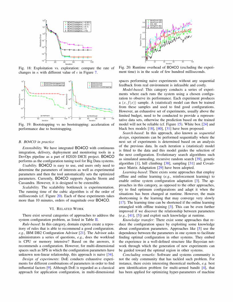
2) Exploitation vs. exploration: In (10), κ adjusts theexploitation-exploration: small κ means high exploitation,while a large κ means a high exploration. The results in Figure17(a) show that using a relatively high exploration (i.e., κ = 8)performs better up to an order of magnitude comparing withhigh exploitations (i.e., κ = 0.1). However, for κ = 0.1, 1exploiting the mean estimates improves the performance atearly iterations comparing with higher explorations cases as inκ = 6. This observation motivated us to tune κ dynamically byusing a lower value at early iterations to exploit the knowledgegained through the initial design and set a higher value lateron, see Section III-C. The result for WordCount in Figure17(b) confirms that adaptive κ improves the performanceconsiderably over constant κ. Figure 18 shows that when weincrease κ with a higher rate (cf. Figure 7), it will improvethe performance. However, the results in Figure 17(a) suggestusing a high value of exploration, this should not be set toan extreme where this makes the mean estimates ineffective.As in Figure 17(a), it performs 4 orders of magnitude worsewhen we ignore the mean estimates (i.e., µt := 0).
3) Bootstrapping vs no bootstrapping: BO4CO uses lhddesign in order to bootstrap the search process. The results for
0 20 40 60 80 100Iteration
10-2
10-1
100
101
102
103
Pre
dic
tion
Err
or
Root Mean Squared Error (RMSE) for BraninRoot Mean Squared Error (RMSE) for Dixon-Szego
0 10 20 30 40 50 60 70 80Iteration
101
102
103
Pre
dic
tion
Err
or
BO4COpolyfit1M5TreeRegressionTreeM5RulesLWP(GAU)PRIM
(a) (b)
Fig. 16: (a) improving accuracy of GP models over time, (b)comparing prediction accuracy of GPs with other machinelearning models on wc(6D).
0 20 40 60 80 100Iteration
10-4
10-3
10-2
10-1
100
101
102
Abso
lute
Err
or
BO4CO(adaptive)BO4CO(µ:=0)BO4CO(κ:=0.1)BO4CO(κ:=1)BO4CO(κ:=6)BO4CO(κ:=8)
0 20 40 60 80 100Iteration
10-3
10-2
10-1
100
101
102
103
104
Abso
lute
Err
or
BO4CO(adaptive)BO4CO(κ:=1)
(a) Branin (b) wc(6D)
Fig. 17: Exploitation vs exploration (a) Branin, (b) wc(6D).
Hartmann and WordCount in Figure 19(a,b) confirms thatthis choice provides a good opportunity in order to explorealong all dimensions and not to trap into local optimumthereafter. However, the results in Figure 19(b) suggest thata high number of initial design may deteriorate the goal offinding the optimum early.
V. DISCUSSIONS
A. Computational and memory requirements
The exact inference BO4CO uses for fitting a GP modelto the t observed data is O(t3) because of inversion ofkernel K−1 in (7). We could in principle compute theCholesky decomposition and use it for subsequent predic-tions, which would lower the complexity to O(t2). However,since in BO4CO we learn the kernel hyper-parameters everyN` iterations, Cholesky decomposition must be re-computed,therefore the complexity is in principle O(t2 × t/N`), wherethe additional factor of t/N` counts the expected number ofiterations. Figure 20 provides the computation time for findingthe next configuration in Algorithm 1 for 5 datasets in TableI. The time is measured running BO4CO on a MacBook Prowith 2.5 GHz Intel Core i7 CPU and 16GB of Memory.The computation time in larger datasets (RollingSort(6D),SOL(6D), WordCount(6D)) is higher than those with lessdata and lower dimensions (WordCount(3,5D)). Moreover,the computation time increases over time since the matrix sizefor Cholesky inversion gets larger.
BO4CO requires to store 3 vectors of size |X| for mean,variance and LCB estimates and a matrix of size |S1:t|×|S1:t|for K and of size |S1:t| for observations, making the memoryrequirement of O(3|X|+ |S1:Nmax |(|S1:Nmax |+ 1)) in total.
0 20 40 60 80 100Iteration
10-4
10-3
10-2
10-1
100
101
102
Absolu
te E
rror
BO4CO(adaptive,ǫ=0.001)BO4CO(adaptive,ǫ=0.01)BO4CO(adaptive,ǫ=0.1)BO4CO(adaptive,ǫ=1)BO4CO(adaptive,ǫ=10)
Fig. 18: Exploitation vs. exploration: compare the rate ofchanges in κ with different value of ε in Figure 7.
0 20 40 60 80 100Iteration
10-4
10-2
100
102
104
Ab
solu
te E
rro
r
BO4CO(3-lhd)BO4CO(9-lhd)BO4CO(no-bootstrapping)
0 50 100 150Iteration
10-3
10-2
10-1
100
101
Ab
solu
te E
rro
r
BO4CO(bootstrapped-lhd)BO4CO(no-bootstrapping)
(a) Hartmann (b) WordCount
Fig. 19: Bootstrapping vs no bootstrapping: acceleration ofperformance due to bootstrapping.
B. BO4CO in practice
Extensibility. We have integrated BO4CO with continuousintegration, delivery, deployment and monitoring tools in aDevOps pipeline as a part of H2020 DICE project. BO4COperforms as the configuration tuning tool for Big Data systems.
Usability. BO4CO is easy to use, end users only need todetermine the parameters of interests as well as experimentalparameters and then the tool automatically sets the optimizedparameters. Currently, BO4CO supports Apache Storm andCassandra. However, it is designed to be extensible.
Scalability. The scalability bottleneck is experimentation.The running time of the cubic algorithm is of the order ofmilliseconds (cf. Figure 20). Each of these experiments takesmore than 10 minutes, orders of magnitude over BO4CO.
VI. RELATED WORK
There exist several categories of approaches to address thesystem configuration problem, as listed in Table II.
Rule-based: In this category, domain experts create a repos-itory of rules that is able to recommend a good configuration.e.g., IBM DB2 Configuration Advisor [21]. The Advisor asksadministrators a series of questions, e.g., does the workloadis CPU or memory intensive? Based on the answers, itrecommends a configuration. However, for multi-dimensionalspaces such as SPS in which the configuration parameters haveunknown non-linear relationship, this approach is naive [34].
Design of experiments: DoE conducts exhaustive experi-ments for different combinations of parameters in order to findinfluential factors [9]. Although DoE is regarded as a classicalapproach for application configuration, in multi-dimensional
0 20 40 60 80 100Iteration
0.15
0.2
0.25
0.3
0.35
0.4
Ela
pse
d T
ime
(s)
WordCount (3D)WordCount (6D)SOL (6D)RollingSort (6D)WordCount (5D)
Fig. 20: Runtime overhead of BO4CO (excluding the experi-ment time) is in the scale of few hundred milliseconds.
spaces performing naive experiments without any sequentialfeedback from real environment is infeasible and costly.
Model-based: This category conducts a series of experi-ments where each runs the system using a chosen configu-ration to observe its performance. Each experiment producesa (x, f(x)) sample. A (statistical) model can then be trainedfrom these samples and used to find good configurations.However, an exhaustive set of experiments, usually above thelimited budget, need to be conducted to provide a represen-tative data sets, otherwise the prediction based on the trainedmodel will not be reliable (cf. Figure 15). White box [24] andblack box models [18], [40], [31] have been proposed.
Search-based: In this approach, also known as sequentialdesign, experiments can be performed sequentially where thenext set of experiments is determined based on an analysisof the previous data. In each iteration a (statistical) modelis fitted to the data and this model guides the selection ofthe next configuration. Evolutionary search algorithms suchas simulated annealing, recursive random search [39], geneticalgorithm [1], hill climbing [38], sampling [31] and Covari-ance Matrix Adaptation [29] have been adopted.
Learning-based: There exists some approaches that employoffline and online learning (e.g., reinforcement learning) toenable online system configuration adaptation [3]. The ap-proaches in this category, as opposed to the other approaches,try to find optimum configurations and adapt it when thesituations has been changed at runtime. However, the mainshortcoming is the learning that may converge very slowly[17]. The learning time can be shortened if the online learningentangled with offline training [3]. This can be even furtherimproved if we discover the relationship between parameters(e.g., [41], [5]) and exploit such knowledge at runtime.
Knowledge transfer: There exist some approaches that re-duce the configuration space by exploiting some knowledgeabout configuration parameters. Approaches like [5] use thedependence between the parameters in one system to facilitatefinding optimal configuration in other systems. They embedthe experience in a well-defined structure like Bayesian net-work through which the generation of new experiments canbe guided toward the optimal region in other systems.
Concluding remarks: Software and systems community isnot the only community that has tackled such problem. Forinstance, there exists interesting theoretical methods, e.g. bestarm identification problem for multi-armed bandit [4], thathas been applied for optimizing hyper-parameters of machine
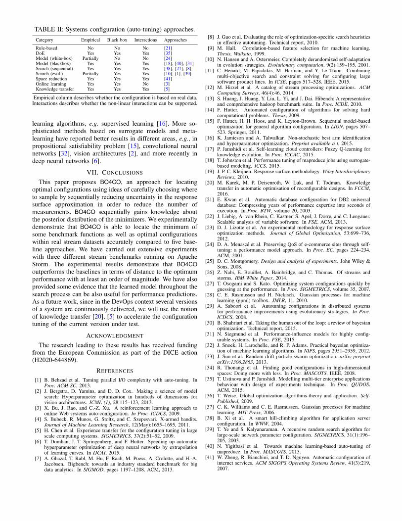
TABLE II: Systems configuration (auto-tuning) approaches.
Category Empirical Black box Interactions Approaches
Rule-based No No No [21]DoE Yes Yes Yes [35]Model (white-box) Partially No No [24]Model (blackbox) Yes Yes Yes [18], [40], [31]Search (sequential) Yes Yes Yes [38], [27], [8]Search (evol.) Partially Yes Yes [10], [1], [39]Space reduction Yes Yes Yes [41]Online learning Yes Yes No [3]Knowledge transfer Yes Yes Yes [5]
Empirical column describes whether the configuration is based on real data.Interactions describes whether the non-linear interactions can be supported.
learning algorithms, e.g. supervised learning [16]. More so-phisticated methods based on surrogate models and meta-learning have reported better results in different areas, e.g., inpropositional satisfiability problem [15], convolutional neuralnetworks [32], vision architectures [2], and more recently indeep neural networks [6].
VII. CONCLUSIONS
This paper proposes BO4CO, an approach for locatingoptimal configurations using ideas of carefully choosing whereto sample by sequentially reducing uncertainty in the responsesurface approximation in order to reduce the number ofmeasurements. BO4CO sequentially gains knowledge aboutthe posterior distribution of the minimizers. We experimentallydemonstrate that BO4CO is able to locate the minimum ofsome benchmark functions as well as optimal configurationswithin real stream datasets accurately compared to five base-line approaches. We have carried out extensive experimentswith three different stream benchmarks running on ApacheStorm. The experimental results demonstrate that BO4COoutperforms the baselines in terms of distance to the optimumperformance with at least an order of magnitude. We have alsoprovided some evidence that the learned model throughout thesearch process can be also useful for performance predictions.As a future work, since in the DevOps context several versionsof a system are continuously delivered, we will use the notionof knowledge transfer [20], [5] to accelerate the configurationtuning of the current version under test.
ACKNOWLEDGMENT
The research leading to these results has received fundingfrom the European Commission as part of the DICE action(H2020-644869).
REFERENCES
[1] B. Behzad et al. Taming parallel I/O complexity with auto-tuning. InProc. ACM SC, 2013.
[2] J. Bergstra, D. Yamins, and D. D. Cox. Making a science of modelsearch: Hyperparameter optimization in hundreds of dimensions forvision architectures. ICML (1), 28:115–123, 2013.
[3] X. Bu, J. Rao, and C.-Z. Xu. A reinforcement learning approach toonline Web systems auto-configuration. In Proc. ICDCS, 2009.
[4] S. Bubeck, R. Munos, G. Stoltz, and C. Szepesvari. X-armed bandits.Journal of Machine Learning Research, 12(May):1655–1695, 2011.
[5] H. Chen et al. Experience transfer for the configuration tuning in largescale computing systems. SIGMETRICS, 37(2):51–52, 2009.
[6] T. Domhan, J. T. Springenberg, and F. Hutter. Speeding up automatichyperparameter optimization of deep neural networks by extrapolationof learning curves. In IJCAI, 2015.
[7] A. Ghazal, T. Rabl, M. Hu, F. Raab, M. Poess, A. Crolotte, and H.-A.Jacobsen. Bigbench: towards an industry standard benchmark for bigdata analytics. In SIGMOD, pages 1197–1208. ACM, 2013.
[8] J. Guo et al. Evaluating the role of optimization-specific search heuristicsin effective autotuning. Technical report, 2010.
[9] M. Hall. Correlation-based feature selection for machine learning.Thesis, Waikato, 1999.
[10] N. Hansen and A. Ostermeier. Completely derandomized self-adaptationin evolution strategies. Evolutionary computation, 9(2):159–195, 2001.
[11] C. Henard, M. Papadakis, M. Harman, and Y. Le Traon. Combiningmulti-objective search and constraint solving for configuring largesoftware product lines. In ICSE, pages 517–528. IEEE, 2015.
[12] M. Hirzel et al. A catalog of stream processing optimizations. ACMComputing Surveys, 46(4):46, 2014.
[13] S. Huang, J. Huang, Y. Liu, L. Yi, and J. Dai. Hibench: A representativeand comprehensive hadoop benchmark suite. In Proc. ICDE, 2010.
[14] F. Hutter. Automated configuration of algorithms for solving hardcomputational problems. Thesis, 2009.
[15] F. Hutter, H. H. Hoos, and K. Leyton-Brown. Sequential model-basedoptimization for general algorithm configuration. In LION, pages 507–523. Springer, 2011.
[16] K. Jamieson and A. Talwalkar. Non-stochastic best arm identificationand hyperparameter optimization. Preprint available a t, 2015.
[17] P. Jamshidi et al. Self-learning cloud controllers: Fuzzy Q-learning forknowledge evolution. In Proc. ICCAC, 2015.
[18] T. Johnston et al. Performance tuning of mapreduce jobs using surrogate-based modeling. ICCS, 2015.
[19] J. P. C. Kleijnen. Response surface methodology. Wiley InterdisciplinaryReviews, 2010.
[20] M. Kurek, M. P. Deisenroth, W. Luk, and T. Todman. Knowledgetransfer in automatic optimisation of reconfigurable designs. In FCCM,2016.
[21] E. Kwan et al. Automatic database configuration for DB2 universaldatabase: Compressing years of performance expertise into seconds ofexecution. In Proc. BTW, volume 20, 2003.
[22] J. Liebig, A. von Rhein, C. Kastner, S. Apel, J. Dorre, and C. Lengauer.Scalable analysis of variable software. In FSE. ACM, 2013.
[23] D. J. Lizotte et al. An experimental methodology for response surfaceoptimization methods. Journal of Global Optimization, 53:699–736,2012.
[24] D. A. Menasce et al. Preserving QoS of e-commerce sites through self-tuning: a performance model approach. In Proc. EC, pages 224–234.ACM, 2001.
[25] D. C. Montgomery. Design and analysis of experiments. John Wiley &Sons, 2008.
[26] Z. Nabi, E. Bouillet, A. Bainbridge, and C. Thomas. Of streams andstorms. IBM White Paper, 2014.
[27] T. Osogami and S. Kato. Optimizing system configurations quickly byguessing at the performance. In Proc. SIGMETRICS, volume 35, 2007.
[28] C. E. Rasmussen and H. Nickisch. Gaussian processes for machinelearning (gpml) toolbox. JMLR, 11, 2010.
[29] A. Saboori et al. Autotuning configurations in distributed systemsfor performance improvements using evolutionary strategies. In Proc.ICDCS, 2008.
[30] B. Shahriari et al. Taking the human out of the loop: a review of bayesianoptimization. Technical report, 2015.
[31] N. Siegmund et al. Performance-influence models for highly config-urable systems. In Proc. FSE, 2015.
[32] J. Snoek, H. Larochelle, and R. P. Adams. Practical bayesian optimiza-tion of machine learning algorithms. In NIPS, pages 2951–2959, 2012.
[33] J. Sun et al. Random drift particle swarm optimization. arXiv preprintarXiv:1306.2863, 2013.
[34] R. Thonangi et al. Finding good configurations in high-dimensionalspaces: Doing more with less. In Proc. MASCOTS. IEEE, 2008.
[35] T. Ustinova and P. Jamshidi. Modelling multi-tier enterprise applicationsbehaviour with design of experiments technique. In Proc. QUDOS.ACM, 2015.
[36] T. Weise. Global optimization algorithms-theory and application. Self-Published, 2009.
[37] C. K. Williams and C. E. Rasmussen. Gaussian processes for machinelearning. MIT Press, 2006.
[38] B. Xi et al. A smart hill-climbing algorithm for application serverconfiguration. In WWW, 2004.
[39] T. Ye and S. Kalyanaraman. A recursive random search algorithm forlarge-scale network parameter configuration. SIGMETRICS, 31(1):196–205, 2003.
[40] N. Yigitbasi et al. Towards machine learning-based auto-tuning ofmapreduce. In Proc. MASCOTS, 2013.
[41] W. Zheng, R. Bianchini, and T. D. Nguyen. Automatic configuration ofinternet services. ACM SIGOPS Operating Systems Review, 41(3):219,2007.
APPENDIX
In this extra material, we briefly describe additional detailsabout the experimental setting and complementary results thatwere not included in the main text.
A. Code and Data
https://github.com/dice-project/DICE-Configuration-BO4CO
B. Documents
https://github.com/dice-project/DICE-Configuration-BO4CO/wiki
C. Configuration Parameters
The list of configuration parameters in Apache Storm thatwe have used in the experiments (cf. Table IV):• max spout (topology.max.spout.pending). The maximum
number of tuples that can be pending on a spout.• spout wait (topology.sleep.spout.wait.strategy.time.ms).
Time in ms the SleepEmptyEmitStrategy should sleep.• netty min wait (storm.messaging.netty.min wait ms).
The min time netty waits to get the control back fromOS.
• spouts, splitters, counters, bolts. Parallelism level.• heap. The size of the worker heap.• buffer size (storm.messaging.netty.buffer size). The size
of the transfer queue.• emit freq (topology.tick.tuple.freq.secs). The frequency at
which tick tuples are received.• top level. The length of a linear topology.• message size, chunk size. The size of tuples and chunk
of messages sent across PEs respectively.
D. Benchmark Settings
Table III represent the infrastructure specification we haveused in the experiments (cf. testbed column in Table IV).
TABLE III: Cluster specification
Cluster Specification
C1 OpenNebula, 3 Sup, 1 ZK, 1 Nimbus, N: (1CPU, 4GB Mem)
C2 EC2, 3 Sup, 1 ZK, 1 Nimbus, N: m1.medium (1 CPU, 3.75GB)
C3 OpenNebula, 3 Sup: (3CPU,6GB Mem), 1 ZK: (1CPU,4GB Mem),1 Nimbus: (2CPU,4GB Mem)
C4 EC2, 3 Sup, 1 ZK, 1 Nimbus, N: m3.large (2CPU, 7.5GB)
C5 Azure, 3 Sup: Standard D1(1CPU, 3.5GB) , 1 ZK, 1 Nimbus,N: Standard A1(1CPU, 1.75GB)
E. Datasets
Note that the parameters with ? shows the interactingparameters. After collecting experimental data, we have useda common correlation-based feature selector implemented inWeka to rank parameter subsets according to a correlationbased on a heuristic. The analysis results demonstrate that inall the 10 experiments at most 2-3 parameters were stronglyinteracting with each other, out of a maximum of 6 parametersvaried simultaneously. Therefore, the determination of the re-gions where performance is optimal will likely to be controlledby such dominant factors, even though the determination of aglobal optimum will still depend on all the parameters.
TABLE IV: Experimental datasets, note that this is the com-plete set of datasets that we experimentally collected over thecourse of 3 months (24/7) for evaluating BO4CO.
Dataset Parameters Size Testbed
1 wc(6D)
?1-spouts: {1,3},?2-max spout: {1,2,10,100,1000,10000},3-spout wait:{1,2,3,10,100},4-splitters:{1,2,3,6},?5-counters:{1,3,6,12},6-netty min wait:{10,100,1000}
2880 C1
2 sol(6D)
?1-spouts:{1,3},?2-max spout:{1,10,100,1000,10000},?3-top level:{2,3,4,5},4-netty min wait:{10,100,1000},5-message size: {10,100,1e3,1e4,1e5,1e6},6-bolts: {1,2,3,6}
2866 C2
3 rs(6D)
1-spouts:{1,3},2-max spout:{10,100,1000,10000},?3-sorters:{1,2,3,6,9,12,15,18},4-emit freq:{1,10,60,120,300},5-chunk size:{1e5,1e6,2e6,1e7},6-message size:{1e3,1e4,1e5}
3840 C3
4 wc(3D)?1-max spout:{1,10,100,1e3, 1e4,1e5,1e6},?2-splitters:{1,2,3,4,5,6},3-counters:{1,2,3,4,5,6,7,8,9,10,11,12,13,14,15,16,17,18}
756 C4
5 wc+rs?1-max spout:{1,10,100,1e3, 1e4,1e5,1e6},?2-splitters:{1,2,3,6},3-counters:{1,3,6,9,12,15,18}
196 C4
6 wc+sol?1-max spout:{1,10,100,1e3, 1e4,1e5,1e6},?2-splitters:{1,2,3,6},3-counters:{1,3,6,9,12,15,18}
196 C4
7 wc+wc?1-max spout:{1,10,100,1e3, 1e4,1e5,1e6},?2-splitters:{1,2,3,6},3-counters:{1,3,6,9,12,15,18}
196 C4
8 wc(5D)
?1-spouts:{1,2,3},2-splitters:{1,2,3,6},3-counters:{1,2,3,6,9,12},4-buffer-size:{256k,1m,5m,10m,100m},5-heap:{“-Xmx512m”, “-Xmx1024m”, “-Xmx2048m”}
1080 C5
9 wc-c1?1-spout wait:{1,2,3,4,5,6,7,8,9,10,100,1e3,1e4},?2-splitters:{1,2,3,4,5,6},3-counters:{1,2,3,4,5,6,7,8,9,10,11,12,13,14,15,16,17,18}
1343 C1
10 wc-c3?1-spout wait:{1,2,3,4,5,6,7,8,9,10,100,1e3,1e4,6e4},?2-splitters:{1,2,3,4,5,6},3-counters:{1,2,3,4,5,6,7,8,9,10,11,12,13,14,15,16,17,18}
1512 C3
F. Performance gainThe performance gain between the worst and best configu-
ration settings are measured for each datasets in Table V.
G. How we set κWe set the exploration-exploitation parameter κ (cf. Figure
7 and boLCB.m in the github repository)) as:
κt =√
2 log(|X|ζ(r)tr/ε), ζ(r) =∞∑n=1
1
nr(13)
where 0 < ε < 1 and r ∈ N, r ≥ 2, ζ(r) is Riemann zeta.
TABLE V: Performance gain between best and worst settings.
Dataset Best(ms) Worst(ms) Gain (%)
1 wc(6D) 55209 3.3172 99%
2 sol(6D) 40499 1.2000 100%
3 rs(6D) 34733 1.9000 99%
4 wc(3D) 94553 1.2994 100%
5 wc(5D) 405.5 47.387 88%