Embed Size (px)
Citation preview

Transport Modeling and Assessment Group
An Overview of the HYSPLIT Modeling System for Trajectory and Dispersion Applications
http://www.arl.noaa.gov/ready/hysplit4.html
Richard S. ArtzMaterial provided by:
Roland Draxler, Mark Cohen, Glenn Rolph, Ariel Stein, and Barbara Stunder
October 22, 2008

Workshop AgendaModel Overview
Model history and featuresComputational methodTrajectories versus concentrationCode installationModel operationExample calculationsUpdating HYSPLIT
Meteorological DataData requirementsForecast data FTP accessAnalysis data FTP accessDisplay grid domainVertical profileContour data
Examples 1-5Particle Trajectory Methods
Trajectory computational methodTrajectory example calculationtrajectory model configurationTrajectory errorMultiple trajectoriesTerrain heightMeteorological analysis along a trajectory
Vertical motion options
Pollutant Plume SimulationsModeling particles or puffsConcentration prediction equationsTurbulence equationsDispersion model configurationDefining multiple sourcesSimulations using emission gridsConcentration and particle display optionsConverting concentration data to text filesExample local scale dispersion calculation
Special TopicsAutomated trajectory calculationsTrajectory cluster analysisConcentration ensemblesChemistry conversion modules
Pollutant depositionSource attribution using back trajectory analysisSource attribution using source-receptor matricesSource attribution functionsGIS Shapefile outputKML/KMZ outputCustomizing map labelsScripting for automated operations
Extra TopicsModeling PM10 emissions from dust stormsRestarting the model from a particle dump file

Transport Modeling and Assessment Group
HYSPLIT Model Features• Predictor-corrector advection scheme; forward or backward integration• Linear spatial & temporal interpolation of meteorology• Converters available ARW, ECMWF, RAMS, MM5, NMM, GFS, …• Vertical mixing based upon SL similarity, BL Ri, or TKE• Horizontal mixing based upon velocity deformation, SL similarity, or TKE• Mixing coefficients converted to velocity variances for dispersion• Dispersion computed using 3D particles, puffs, or both simultaneously• Modelled particle distributions (puffs) can be either Top-Hat or Gaussian• Air concentration from particles-in-cell or at a point from puffs• Multiple simultaneous meteorology and concentration grids• Latitude-Longitude or Conformal projections supported for meteorology• Nested meteorology grids use most recent and finest spatial resolution• Non-linear chemistry modules using a hybrid Lagrangian-Eulerian exchange• Standard graphical output in Postscript, Shapefiles, or Google Earth (kml) • Distribution: PC and Mac executables, and UNIX (LINUX) source

Some Example Applications
• Source region identification


Methodology
205 episodes identified from 14 sites in the Toronto region: 139 PM + 66 O3
Multiple 72-hr back-trajectories were run with the NOAA HYSPLIT model for each episode, starting at the middle of the mixed layer:
24-hr PM episodes: 7 trajectories run for each episode, once every 4 hours (at 0, 4, 8, 12, 16, 20, and 24 hours after the start of the episode)
8-hr O3 episodes: 5 trajectories run for each episode, once every 2 hours (at 0, 2, 4, 6, and 8 hours after the start of the episode)
Following the above methodology, a total of 1303 back-trajectorieswere attempted
Preliminary cluster analysis performed for each group of sites, for PM and O3 episodes
Preliminary analysis of gridded trajectory frequency performed for each group of sites for PM and O3 episodes


Summary of Clustering results for Toronto group (group #1) PM events
As one increases the number of clusters, a point of “diminishing returns” is reached in terms of reducing the “scattering” around the group of clusters
3 cl
uste
rs5
clus
ters
7 cl
uste
rs
The “TSV” is a measure of the degree to which the chosen clusters fit all the data

Results for3 clusters

Another way to look at the universe of back-trajectory results is to determine the fraction of trajectories that pass through a given grid square (in this case a 1o x 1o grid). Here is an example for the overall results for 984 back trajectories run for the PM episodes at sites in the Toronto group.

Ozone events for the “Toronto” group of monitoring sites

another example of grid-frequency results:
Ozone events for the “Eastern” group of monitoring sites

Some Example Applications
• Source region identification• Site selection and data interpretation

5 km
PatuxentRiver
Beltsville Atmospheric Monitoring Site
(EPA, NOAA, State of MD, Univ. of MD)
Patuxent Research Refuge (FWS)
Patuxent Wildlife Research Center
(USGS)
Beltsville Agricultural
Research Center (USDA)
Howard University Atmos. Site ( + NASA, NSF, NOAA, others)

rural AQS
NADP/MDN
CASTNet
IMPROVE
Monitoring sites
other AQS
Hg site
100 miles from DC
the region between the 20 km and 60 km radius circles displayed around the monitoring site might be considered the “ideal”location for sources to be investigated by the site
Bremo
Beltsville monitoring site
Morgantown
Chalk Point
Dickerson
Possum Point
Large Incinerators: 3 medical waste,
1 MSW, 1 haz waste(Total Hg ~ 500 kg/yr)
Brunner Island
Eddystone
Arlington - Pentagon MSW Incin
Brandon Shores and H.A. Wagner
Montgomery CountyMSW Incin
Harford County MSW Incin
coal
incinerator
metals
manuf/other
Symbol colorindicates typeof mercury source
1 - 5050 - 100
100 - 200
200 – 400
400 - 700
700 – 1000
> 1000
Symbol size andshape indicates 1999 mercuryemissions, kg/yr

Beltsville Episode January 7, 2007
07:
30 0
8:30
09:
30 1
0:30
11:
30 1
2:30
13:
30 1
4:30
15:
30 1
6:30
(Eastern Standard Time)January 7, 2007
0
20
40
60
80
100
RG
M (p
g/m
3)
Sometimes, we see evidence of local and regional “plume” impacts

Sometimes, we see evidence of local and regional “plume” impacts
07:
30 0
8:30
09:
30 1
0:30
11:
30 1
2:30
13:
30 1
4:30
15:
30 1
6:30
(Eastern Standard Time)January 7, 2007
0
20
40
60
80
100
RG
M (p
g/m
3)
07:
30 0
8:30
09:
30 1
0:30
11:
30 1
2:30
13:
30 1
4:30
15:
30 1
6:30
(Eastern Standard Time)January 7, 2007
0
20
40
60
80
100
RG
M (p
g/m
3)
07:
30 0
8:30
09:
30 1
0:30
11:
30 1
2:30
13:
30 1
4:30
15:
30 1
6:30
(Eastern Standard Time)January 7, 2007
0
20
40
60
80
100
RG
M (p
g/m
3)
07:
30 0
8:30
09:
30 1
0:30
11:
30 1
2:30
13:
30 1
4:30
15:
30 1
6:30
(Eastern Standard Time)January 7, 2007
0
20
40
60
80
100
RG
M (p
g/m
3)
07:
30 0
8:30
09:
30 1
0:30
11:
30 1
2:30
13:
30 1
4:30
15:
30 1
6:30
(Eastern Standard Time)January 7, 2007
0
20
40
60
80
100
RG
M (p
g/m
3)
07:
30 0
8:30
09:
30 1
0:30
11:
30 1
2:30
13:
30 1
4:30
15:
30 1
6:30
(Eastern Standard Time)January 7, 2007
0
20
40
60
80
100
RG
M (p
g/m
3)
07:
30 0
8:30
09:
30 1
0:30
11:
30 1
2:30
13:
30 1
4:30
15:
30 1
6:30
(Eastern Standard Time)January 7, 2007
0
20
40
60
80
100
RG
M (p
g/m
3)
07:
30 0
8:30
09:
30 1
0:30
11:
30 1
2:30
13:
30 1
4:30
15:
30 1
6:30
(Eastern Standard Time)January 7, 2007
0
20
40
60
80
100
RG
M (p
g/m
3)
07:
30 0
8:30
09:
30 1
0:30
11:
30 1
2:30
13:
30 1
4:30
15:
30 1
6:30
(Eastern Standard Time)January 7, 2007
0
20
40
60
80
100
RG
M (p
g/m
3)
07:
30 0
8:30
09:
30 1
0:30
11:
30 1
2:30
13:
30 1
4:30
15:
30 1
6:30
(Eastern Standard Time)January 7, 2007
0
20
40
60
80
100
RG
M (p
g/m
3)

Some Example Applications
• Source region identification• Site selection and data interpretation• Source attribution

one Hg emissions
source
Beltsville monitoring
site
Model-predicted hourly mercury deposition (wet + dry) in the vicinity of one example Hg source for a 3-day period in July 2007
100 - 100010 – 1001 - 10
0.1 – 1
* hourly deposition convertedto annual equivalent
deposition(ug/m2)*
Washington D.C.

one Hg emissions
source
Beltsville monitoring
site
Model-predicted hourly mercury deposition (wet + dry) in the vicinity of one example Hg source for a 3-day period in July 2007
100 - 100010 – 1001 - 10
0.1 – 1
* hourly deposition convertedto annual equivalent
deposition(ug/m2)*
Washington D.C.

one Hg emissions
source
Model-predicted hourly mercury deposition (wet + dry) in the vicinity of one example Hg source for a 3-day period in July 2007
100 - 100010 – 1001 - 10
0.1 – 1
* hourly deposition convertedto annual equivalent
deposition(ug/m2)*
Washington D.C.
Large, time-varying spatial gradients in deposition & source-receptor relationships
Beltsville monitoring
site

Some Example Applications
• Source region identification• Site selection and data interpretation• Source attribution• Estimation of deposition by source

2002 U.S. and Canadian Emissions of Total Mercury [Hg(0) + Hg(p) + RGM]
Large Point Sources of Mercury Emissions Based on the 2002 EPA NEI and2002 Envr Canada NPRI*
size/shape of symbol denotes amount of mercury emitted (kg/yr)
5 - 1010 - 5050 - 100
100 – 300
300 - 500
500 - 1000
color of symbol denotes type of mercury source
coal-fired power plants
other fuel combustion
waste incineration
metallurgical
manufacturing & other
1000 - 3000
* Note – some large Canadian point sources may not be included due to secrecy agreements between industry and the Canadian government.

Atmospheric Deposition Flux to Lake Michigan from Anthropogenic Mercury Emissions Sources in the U.S. and Canada

Pleasant PrairieJoliet 29
J.H. CampbellWaukegan
MARBLEHEAD LIME CO.Will County
JERRITT CANYON LWD
South Oak CreekPowerton
Superior Special ServicesCLARIAN HEALTHCrawfordR.M. Schahfer Joliet 9Rockport
Marblehead Lime (South Chicago)BALL MEMORIAL FiskState LineEdgewaterVULCAN MCCOOK LIMEMonroe Power PlantMonticelloParkview Mem. Hosp.
WI IL
MI IL IL IL NV KY WI IL WI IN IL IN IL IN IL IN IL IN WI IL MI TX IN
0% 20% 40% 60% 80%Cumulative Fraction of Hg Deposition
0
5
10
15
20
25
Ran
k
coal-fired elec genother fuel combustionwaste incinerationmetallurgicalmanufacturing/other
Top 25 modeled sources of atmospheric mercury to Lake Michigan(based on 1999 anthropogenic emissions in the U.S. and Canada)

0 - 100100 - 200
200 - 400400 - 700
700 - 10001000 - 1500
1500 - 20002000 - 2500
> 2500
Distance Range from Lake Michigan (km)
0
10
20
30
40
50
Emis
sion
s (m
etric
tons
/yea
r)
0
1
2
3
4
5
Dep
ositi
on F
lux
(ug/
m2-
year
)
Emissions Deposition Flux
Emissions and deposition to Lake Michigan arising from different distance ranges
(based on 1999 anthropogenic emissions in the U.S. and Canada)
Only a small fraction of U.S. and Canadian emissions are emitted within 100 km of Lake Michigan…
… but these “local” emissions are responsible for a large fraction of the modeled atmospheric deposition

NOAA Report to Congress on Mercury Contamination in the Great Lakeshttp://www.arl.noaa.gov/data/web/reports/cohen/NOAA_GL_Hg.pdf
The Conference Report accompanying the consolidated Appropriations Act, 2005 (H. Rpt. 108-792) requested that NOAA, in consultation with the EPA, report to Congress on mercury contamination in the Great Lakes, with trend and source analysis.
Reviewed by NOAA, EPA, DOC, White House Office of Science and Technology Policy, and Office of Management and Budget (OMB).
Review process took ~2 years.
Transmitted to Congress on May 14, 2007


Some Example Applications
• Source region identification• Site selection and data interpretation• Source attribution• Estimation of deposition by source• Asian dust and wildfire smoke

Transport Modeling and Assessment Group
China April 2001Particle Distribution and TOMS Aerosol Index
April 7th 0600 UTC April 14th 0600 UTC

Transport Modeling and Assessment Group
Wild Fire Smoke Verificationhttp://www.arl.noaa.gov/smoke


Transport Modeling and Assessment Group
What’s in the pipeline for version 4.9 …
• Web interactive verification linked to DATEM• Integrated global model for background contributions• Chemical (CAMEO) and radiological effects database• GIS-like map background layers for graphical display • Model physics ensemble
– meteorology and turbulence already in existing version• Completely revised user’s guide with examples

National Oceanic and Atmospheric AdministrationAir Resources Laboratory

Extras
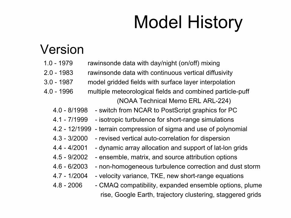
Model HistoryVersion 1.0 - 1979 rawinsonde data with day/night (on/off) mixing2.0 - 1983 rawinsonde data with continuous vertical diffusivity3.0 - 1987 model gridded fields with surface layer interpolation4.0 - 1996 multiple meteorological fields and combined particle-puff
(NOAA Technical Memo ERL ARL-224)4.0 - 8/1998 - switch from NCAR to PostScript graphics for PC4.1 - 7/1999 - isotropic turbulence for short-range simulations4.2 - 12/1999 - terrain compression of sigma and use of polynomial4.3 - 3/2000 - revised vertical auto-correlation for dispersion4.4 - 4/2001 - dynamic array allocation and support of lat-lon grids4.5 - 9/2002 - ensemble, matrix, and source attribution options4.6 - 6/2003 - non-homogeneous turbulence correction and dust storm4.7 - 1/2004 - velocity variance, TKE, new short-range equations4.8 - 2006 - CMAQ compatibility, expanded ensemble options, plume
rise, Google Earth, trajectory clustering, staggered grids

Transport Modeling and Assessment Group
Integration Methods
• Eulerian– Local derivative– Solve over the entire domain– Ideal for multiple sources– Easily handles complex chemistry – Problems with artificial diffusion
• Lagrangian - HYSPLIT– Total derivative– Solve only along the trajectory– Ideal for single point sources– Implicit linearity for chemistry– Non-linear solutions available– Not as efficient for multiple sources

Transport Modeling and Assessment Group
Sensitivity to Particle Number - Why Puff Dispersion?
500 3D-particles• A puff simulation models the growth of
the particle distribution, the particle standard deviation
• Requires fewer puffs than particles to represent distribution
• Puff growth uses the same turbulence parameters as particle method
• The Puff-Particle Hybrid method– Fewer puffs required for horizontal
distribution– Vertical shears captured more
accurately by particles

Transport Modeling and Assessment Group
HYSPLIT Default Deposition Configuration
• Dwet+dry = M [ 1 - exp (-∆t { βdry + βgas + βinc + βbel } ) ]
• Dry Deposition– βdry = Vd / ∆Zp– Vd user defined; Vd = Vg; Resistance method– Vg gravitational settling (Stokes equation)
• Cloud Layer Definition– Cloud bottom: 80% Rh– Cloud top: 60% Rh
• Particle Wet Deposition– Within cloud: βinc = Vinc / ∆Zp; Vinc = S P; S=3.2 x 10⁵
– Below cloud: βbel = 5x10⁻⁵ s-1
• Gaseous Wet Deposition– βgas = Vgas / ∆Z; Vgas = H R T P 103

Transport Modeling and Assessment Group
Representation of a Plume using Trajectories
• A single trajectory cannot properly represent the growth of a pollutant cloud when the wind field varies in space and height
• The simulation must be conducted using many pollutant particles
• In the illustration on the right, new trajectories are started every 4-h at 10, 100, and 200 m AGL to represent the boundary layer transport
• It looks like a plume because wind speed and direction varies with height in the boundary layer

Transport Modeling and Assessment Group
Trajectory based Plume Simulation Options
• Particle: a point mass of contaminant. A fixed number is released with mean and random motion.
• Puff: a 3-D cylinder with a growing concentration distribution in the vertical and horizontal. Puffs may split if they become too large.
• Hybrid: a circular 2-D object (planar mass, having zero depth), in which the horizontal contaminant has a “puff”distribution and in the vertical functions as a particle.

Model HistoryVersion 1.0 - 1979 rawinsonde data with day/night (on/off) mixing2.0 - 1983 rawinsonde data with continuous vertical diffusivity3.0 - 1987 model gridded fields with surface layer interpolation4.0 - 1996 multiple meteorological fields and combined particle-puff
(NOAA Technical Memo ERL ARL-224)4.0 - 8/1998 - switch from NCAR to PostScript graphics for PC4.1 - 7/1999 - isotropic turbulence for short-range simulations4.2 - 12/1999 - terrain compression of sigma and use of polynomial4.3 - 3/2000 - revised vertical auto-correlation for dispersion4.4 - 4/2001 - dynamic array allocation and support of lat-lon grids4.5 - 9/2002 - ensemble, matrix, and source attribution options4.6 - 6/2003 - non-homogeneous turbulence correction and dust storm4.7 - 1/2004 - velocity variance, TKE, new short-range equations4.8 - 2006 - CMAQ compatibility, expanded ensemble options, plume
rise, Google Earth, trajectory clustering, staggered grids
Dry and wet deposition of the pollutants in the puff are estimated at each time step.
The puff’s mass, size, and location are continuously tracked…
Phase partitioning and chemical transformations of pollutants within the puff are estimated at each time step
= mass of pollutant(changes due to chemical transformations and deposition that occur at each time step)
Centerline of puff motion determined by wind direction and velocity
Initial puff location is at source, with mass depending on emissions rate
TIME (hours)0 1 2
deposition 1 deposition 2 deposition to receptor
lake
Lagrangian Puff Atmospheric Fate and Transport Model