1

An overview of numerical methodologies for durability assessment of

vehicle and transport structures

Abstract: Numerical methodologies for assessing the durability of vehicle and transport structures are reviewed. These methodologies are mapped in terms of a framework that emphasizes the relationships among them. Load inputs are obtained from either measurements or simulation. These loads are used as inputs into stress analyses, which may be either quasi-static or dynamic, and either in the time domain or in the frequency domain. The outputs of these analyses can then be used in fatigue analyses. The advantages and disadvantages of each method are analysed. A case study is described to demonstrate the insights gained from the mapping framework. Keywords: Durability assessment, fatigue analysis, input loading, vehicle design, vehicle and transport structure

1 Introduction The constant drive in the vehicle and transport equipment manufacturing industries to shorten design cycle times and reduce development cost have caused an ever increasing emphasis on numerical techniques, rather than the physical testing of prototypes. To this end, a plethora of methods and methodologies have been developed over past decades. Generically the process of numerical durability assessment involves: deriving the input loading from measurements or simulation, computing the stress/strain response to the input loading and predicting fatigue life on the basis of the calculated stress/strain responses and material properties. Each of these stages may involve various specialist methods and methodologies. Designers and structural analysts are therefore increasingly faced with a series of complex considerations and decisions when attempting to map a way through the growing suite of methods and methodologies available for all of these process stages. In the literature there are a number of compendiums and reviews presenting these methodologies and discussing their advantages, disadvantages and applications. In a typical flow diagram in the SAE Fatigue Design Handbook (1997), the durability assessment process is divided into experimental components and analytical/numerical components. The experimental components are the service history determination, strain measurements and structural life testing, whereas the analytical components are multi-body dynamic simulation, numerical stress analysis and fatigue life prediction. The same source provides a flow diagram depicting a more detailed process of predicting fatigue life. Here the logic of requiring loads (as well as material properties and geometry) to perform structural analysis, the outputs of which may be used to analyse crack initiation or crack propagation, is apparent but the different methods for determining the loads, the various structural analysis techniques or the choices of methods to perform initiation analysis, are not represented. The handbook does deal comprehensively with these aspects in the text, although it does not address the themes of dynamic versus static finite element analyses, nor frequency domain versus time domain analyses. This and other similar sources (e.g. Berger et al., 2002) do not offer an integrated, holistic representation of the durability assessment process, applicable to the entire ground-vehicle

2

industry, but with sufficient detail so as to include as components the different choices of methods for determining input loading, performing stress analysis and performing fatigue analysis, as well as to represent the various permutations of methods that would be viable for performing durability assessment. This paper proposes a framework for mapping numerical methods and methodologies for the durability assessment of vehicle and transport structures. The mapping framework offers a concise, integrated and holistic view of the subject matter and enables a high-level evaluation of the various methodologies. The insight provided by the framework, as well as the evaluation scheme, is then demonstrated by means of a case study.

2 Components of mapping framework Figure 1 outlines the proposed mapping framework. The framework may logically be divided into three vertical regions. The components of this framework are developed in the following. This is best accomplished by commencing with a description of stress analysis methods (centre region), followed by an analysis of methods to determine the appropriate input loading (top region), and then considering fatigue analysis methods (bottom region).

3

Figure 1 Outline of Mapping Framework

The populated framework is depicted in Figure 2.The components of the framework are identified in italics in the text below.

2.1 Stress analysis The stress analysis methods used in vehicle and transport structure durability assessment may be classified as either quasi-static or dynamic methods, as well as being either in the time domain or in the frequency domain. The rationale for these classifications will become apparent in the subsequent sections.

2.1.1 Quasi-static finite element analysis The basic method for quasi-static finite element analysis described by Bishop and Sherratt (2000), involves calculating the stress response σij for all (or critical) elements i, caused by applying static unit loads Lj-uni at nodes j, one at a time, for all significant loads acting on the structure. This calculation is made by using the static finite element method (Static FEA in the classification framework presented in Figure 2). These results are used to establish a quasi-static transfer matrix [K] between element stresses and loads (critical. position / load transfer matrix in framework). The known time histories of each load Lj(t) are then multiplied by the inverse of the transfer matrix, achieving, through superposition, the stress time histories σi(t) at each element i:

Eq. 1 This method is classified as quasi-static, since, although the stress response to dynamic loading is calculated, it is achieved without solving the equilibrium equation containing the mass and damping matrices (Eq. 4 below). This method is classified as a time domain method, since the stresses are calculated in the time domain.

Measurements

Quasi-static Dynamic

STRESS ANALYSIS

Simulation

LOAD INPUT

FATIGUE ANALYSIS

Freq. domain Time domain Time domain

4

2.1.2 Co-variance method Dietz et al. (1998) describe a method which employs a dynamic simulation model of a train to establish the dynamic loads on a bogey. Quasi-static, as well as condensed dynamic finite element analyses, are then performed to obtain the stress histories for subsequent fatigue analysis. A stress load matrix [B] is calculated for only the critical areas of concern, with

Eq. 2

where [σc(t)] are the stress tensors at the critical locations, [L(t)] are the various input loads (forces and accelerations as functions of time) and [B] contains the stress tensor results from static unit load analyses for each input load, as well as the modal stresses obtained from eigenvalue finite element analysis. Eq. 2 is equivalent to Eq. 1 with [B] = [K]-1. The time-independent stress load matrix allows the load covariance matrix to be transformed into a stress covariance matrix:

Eq. 3 Although the resulting stress covariance matrix contains only the information about the amplitude distribution of stresses, the number of cycles can be derived by assuming a probability density function for a stationary random process, allowing fatigue analyses to be performed at the critical positions. This approach therefore represents a quasi-static method in the frequency domain, although inputs are required from a dynamic eigenvalue finite-element analysis.

5

Figure 2 Mapping framework for durability assessment methodologies

Part of more than one methodology RPA methodology Random vibration methodology Covariance methodology Direct integration methodology FDRS methodology Time-domain modal superposition FESL methodology

Freq. domain

Measurements Simulation

Quasi-static Dynamic STRESS ANALYSIS

LOAD INPUTS

FATIGUE ANALYSIS

Freq. domain Time domain Time domain

Multi-body dynamic simulation Unit load

Strain gauge / Load transfer matrix

L(t) Road profiles

a(t)

FFT/PSD

σ(t), ε(t)

Single DOF Response

Rainflow counting

Stress life FESL Strain life Fracture mechanics

Dirlik formula Material properties

FDRS curves

Static FEA

Transient dynamic direct integration

Eigenvalue FEA

Critical position / load transfer matrix Modal

superposition

Large mass, relative inertial, or Lagrange multipliers

Covariance method

6

2.1.3 Eigenvalue finite element analysis Eigenvalue FEA is the basis of several frequency domain methods (quasi-static, as described in the previous paragraph, as well as dynamic). It entails employing the finite element technique to solve for the natural frequencies and mode-shapes of a structure by computing the eigenvalues of the equilibrium equations, as described by Bathe (1996). A dynamic system may be described by the following equilibrium equation:

Eq. 4

where is the displacement vector, the mass matrix, the damping matrix, the stiffness matrix and the load vector. The eigenvalue analysis solves for the natural frequencies ωr and modes φr of the system, by solving the following equation:

Eq. 5

The modes are then collected to form the modal matrix, [Φ] = [φ1 φ2 φ3 …….].

2.1.4 Transient dynamic direct integration method Dynamic finite-element analysis entails solving for the displacements in Eq. 4. One group of methods uses the direct integration method (that Bishop and Sherratt (2000) call dynamic transient analysis) to solve for the displacements after each small time increment by direct integration (therefore a dynamic method in the time domain). A complete analysis is therefore performed at each time step, except for the compilation of the mass, damping and stiffness matrices, which need only be computed once.

2.1.5 Modal superposition Modal superposition involves the superposition of the mode shapes that participate in the forced response, calculated in either the time domain or the frequency domain (therefore depicted on both sides of the time domain / frequency domain division line in Figure 2. The economy of the method is derived from the possibility of truncating the modes required to converge to an accurate solution. A method with superior convergence properties is the mode-acceleration method (MAM), described by Rixen (2001). A solution for the standard equations of motion (without damping)

Eq. 6 can be expressed as follows:

Eq. 7 where the are the principal co-ordinates and is the number of truncated modes. The first term in the above equation represents the quasi-static (or non-modal) response, with a linear relationship between the load history and the displacement response. The stress response can be calculated from the displacement response, also using a linear relationship, implying that this term yields results equivalent to those that would be obtained from Eq. 1. The second term superimposes the effects of the truncated modes that may participate in the full dynamic response.

7

2.1.6 Summary of stress analysis methods As is clear from the above discussion, dynamic finite-element analysis of vehicle structures is not a trivial problem. There are several choices of the method to apply, depending mainly on the type of input data available. Generally, it is not practical to perform dynamic analyses to obtain fatigue stresses, unless stationary random data is assumed, and/or the model is condensed. Careful planning is required for the measurements taken to obtain input data for these analyses. For considerations of economy as well as the fact that the requirements for dynamic analysis are generally too complex for inclusion in design codes and standards, quasi-static methods are mostly employed.

2.2 Load inputs Grubisic (1994) states that the service life of a vehicle component depends decisively on the loading conditions during service. It is necessary to define a representative loading profile for both design and testing purposes. If this is not defined, the most sophisticated analysis or testing techniques will yield no useful results. This section describes some of the important current practices in this regard. In most cases, inputs for dynamic analyses are obtained from measurements. On vehicles, the parameters that are typically measured are the accelerations, displacements and/or forces, as well as strains, described in the paragraphs below, followed by a discussion on deriving input loads using multi-body dynamic simulation.

2.2.1 Force inputs When forces should be measured, the equilibrium equation (Eq. 4), can be directly solved, since the unknown displacements are on one side of the equation. The measured forces, represented by the block in the framework, are used as inputs into the various methods. Gopalakrishnan and Agrawal (1993) describe the measurement of triaxial (vertical, longitudinal, lateral) wheel forces, using a specially developed loadcell which takes the place of the wheel hub. Standardized load-time histories are an important source of load inputs for testing and analysis in the automotive industry. Berger et al. (2002) discuss a number of these, e.g. CARLOS, which provides load sequences for vertical, longitudinal and lateral forces on car suspensions, based on measured data from collaborators in the German automotive industry.

2.2.2 Acceleration inputs It is difficult to measure directly the forces introduced through the suspension of a vehicle to the vehicle structure, because such measurement requires special loadcells. Accelerations are often measured. In this case the direct solving of the equilibrium equation (Eq. 4) is not possible, since prescribed motion terms are part of the vector on the left-hand side of the equation. Three methods are commonly used to circumvent these problems (MSC/NASTRAN User’s Guide): • Large mass-spring method

This method entails adding an element with a large mass or stiffness at the point of known acceleration. Large forces, calculated as the large mass multiplied by the desired accelerations (or stiffness multiplied by known displacements) are applied to obtain the required motion. The method is not exact, since it is based on the assumption that the inertia of the large mass will dominate the displacement of the load application node, compared to the influences of other stiffnesses and inertias, and may produce various errors if used with the inputs required at more than one point.

• Relative displacement method

8

This method entails input accelerations defined as the inertial motion of a rigid base to which the structure is connected. The structural displacements are then calculated relative to the base motion.

• Lagrange multiplier technique This technique requires adding additional degrees of freedom to the matrix solution, that are used as force variables for the constraint functions. Coefficients are added to the matrices for the equations that couple the constrained displacement variables to the points at which enforced motion is applied. The technique produces indefinite system matrices that require a special resequencing of variables for numerical stability.

2.2.3 Strain measurements Strain measurements (represented by the σ(t), ε(t) block in the framework, since the measured strains are usually converted to stresses), are commonly used to derive input loads for stress and fatigue analyses, since it is less expensive than measurement exercises requiring specialized loadcells and it also avoids the difficulties with acceleration measurements, described in the previous paragraph. Since strain measurements entail the measurement of the structural response, rather than the input loading, a technique is required to derive the input loading from the response data. This input loading is derived by compiling a strain gauge / load transfer matrix from static finite element analyses with unit loads, which, when inverted, can be used to calculate the time histories of loads. This technique forms part of a comprehensive methodology, described in more detail in paragraph 3.1.

2.2.4 Multi-body dynamic simulation Multi-body dynamic simulation is an important technique to establish dynamic input loading for vehicle structures when measurements are not feasible. A dynamic (mass-spring-damper) model of the vehicle system is constructed. The traversing of the vehicle over a terrain with known statistical or geometric profiles (such as digitized proving-ground section profiles) is then simulated to solve for the dynamic input loading. These loads may then be applied to finite element models. Examples of this process are reported by Oyan (1998), where the fatigue life of a railway bogie and a passenger train structure is predicted by using dynamic simulation. For trackless vehicles, one of the fundamental difficulties with the accurate dynamic simulation of input loads is related to the complexity of modelling the tyres. Captain et al. (1979) describe analytical tyre models and Faria et al. (1992) discuss tyre modelling by finite-element methods. Mousseau states in the SAE Fatigue Design Handbook (1997) that simplified tyre models may lead to significant errors in simulating durability loading. Dynamic simulation is often employed to solve for the high number of loads acting on body attachment locations when assessing the durability of a complete body structure of a vehicle using finite element methods, because of the practical difficulties with measuring these loads (Gopalakrishnan and Agrawal, 1993). Measured wheel loads, using a specialized loadcell, are introduced to a dynamic model, which then solves for the attachment point loads. A similar process may be followed, using measured wheel accelerations (Conle and Chu, 1991), but difficulties are usually encountered with the double integration of the acceleration signals to obtain displacements.

9

2.2.5 Summary of input loading Measurements as a source for input loading can only be taken if a prototype or a similar vehicle is available. The direct measurement of input forces using loadcells (or strain-gauged components calibrated as loadcells) would be preferable, since it avoids the complexities of deriving loads from remote strain-gauge measurements, or accelerometers. However, this may often be expensive or impractical. Three types of applications are identified for multi-body dynamic simulation in the durability assessment process. These types, as well as the purpose, input required and difficulties, are summarized in Table 1. Table 1: Types of dynamic simulation applications

2.3 Fatigue analysis The final step in the durability assessment process entails predicting the fatigue life of critical areas of the structure. The various fatigue analysis methods described below require an intermediate step, to convert the frequency domain or time domain stress histories, to stress ranges and numbers of cycles. Methods of cycle counting are discussed first. All the fatigue analysis methods also require material properties as inputs, as shown in the diagram.

2.3.1 Cycle counting

2.3.1.1 Rainflow counting The original logic of this method was based on the extraction of closed hysteresis loops from the elastic-plastic stress-strain history, as depicted in Figure 3. An algorithm which is easily computerized, also called the range-pair-range method, is described in ASTM E 1049-85 (1989). The outcome of the cycle counting according to this method for the idealized signal depicted below, would be two cycles with the same stress range, though different means (the two black cycles), as well as one large cycle (the grey cycle).

Figure 3 Rainflow counting

10

Dressler and Kottgen (1999) summarize cycle-counting methods for multi-axial, non-proportional loading. The intention is to count cycles so that a multi-axial fatigue calculation (e.g. according to the critical plane approach) can be performed from reconstructed data. The process of calculating the fatigue damage caused by random loading is normally based on the linear damage accumulation approach, proposed by Miner (1945). The total damage D caused by a combination of cycles of different ranges is calculated as the linear sum of the fraction of the applied number of cycles at that range ni divided by the number of cycles to failure at that range Ni. Failure is expected if the total damage reaches unity.

Eq. 8 A large number of alternative or adapted models for damage accumulation have been developed. A survey of these models is presented by Fatemi and Yang (1998). Six categories of methods are defined:

• Linear damage summation • Two-stage linear and non-linear damage curves • Life curve modifications to account for load interactions • Approaches based on fracture mechanics crack growth • Models based on continuum damage mechanics • Energy-based methods

It is stated that no model is universally accepted, since each model accounts for particular factors, such as load sequence effects, non-linear damage evolution, mean stress, overload effects or small cycles below fatigue limit. For this reason, the Miner approach is still predominantly used, despite major shortcomings. It may also be argued that numerical fatigue assessments in the vehicle industries are often performed on a relative basis, implying that the need for accurate life predictions in an absolute sense is not required. The Miner approach is best suited to such cases.

2.3.1.2 Frequency domain fatigue life Methods for estimating fatigue life from frequency domain data are described by Sherratt (1996). Although the fatigue failure mechanism depends essentially on amplitudes and the number of occurrences (parameters determined through cycle counting from time domain data), the restrictions of data storage space and communication often imply the need to find more compact data formats, such as the direct storage of real-time cycle count results, or the statistical information represented by the frequency domain. Data stored in a power spectral density (PSD) format represents the averaged statistical information about the energy contained in the original time-domain signal at each frequency. Since the energy will be related to amplitudes and the frequencies to the number of cycles, intuitively it should be possible to calculate fatigue damage. Sherratt (1996) describes the Dirlik formula which estimates the probability density function (PDF) of rainflow ranges as a function of moments of the PSD. This formula is empirically derived from the results of the IFFTs of a number of PSDs with random phases. This formula allows the closed-form estimation of fatigue damage from PSD data. It is important to note that a fundamental assumption made when using frequency domain data is that the time data is stationary, meaning that PSDs taken on any partial duration of the data will

11

be similar. This may be true for data obtained from a vehicle travelling on a road of constant roughness, but will certainly exclude transient events, such as hitting a curb. Usually, such transient events are then additionally considered in the time domain.

2.3.2 Stress-life approach The stress-life approach is described by Bannantine et al. (1990). The approach is based on the response curve experimentally established for material fatigue, called the SN curve, which plots the number of cycles N or reversals 2N to failure (mostly defined as the initiation of an observable crack) versus a nominal stress range Δσ or amplitude σa. For most metallic materials used in the vehicle and transport equipment industries, an approximate straight line may usually be observed on a log-log plot, resulting in a power-law relationship:

Eq. 9 where Sf is the fatigue coefficient and b is the fatigue exponent. The fatigue analysis of the welded components that are very important in vehicular structures, is based on the original work done by Gurney (1976). SN-curves, equivalent to the material properties used in the stress-life method, are derived from extensive tests performed on different specimens of weld joints. Numerous fatigue design standards or codes are based on the above method, e.g. International Institute of Welding document, Hobbacher (1996). Leever (1983) and Stephens et al. (1987) describe methods using ‘hot-spot’ stress for fatigue calculations. This is of importance when having to analyse a complex joint which cannot be classified according to the design codes. The hot-spot stress is the maximum principal stress at the weld toe, which can be calculated by finite element analysis with solid elements, and considers the weld geometry. Pettersson (2002) reports on a project involving a comparison of four different fatigue analysis methods for welded components, as well as experimental results. Two of the methods are described above, namely the stress-life method using SN-curves based on nominal stresses and the hot-spot stress method (called the effective notch-stress method by Pettersson), which uses the maximum stress at the weld toe, calculated by means of an assumed weld toe radius (typically 1 mm). An intermediate method, which Pettersson calls the geometric stress method, includes all stress-raising effects except for the weld toe geometry, and is calculated by not modelling the weld geometry and extrapolating to the position of the weld toe the stress transient close to the weld. The fourth method is based on Linear Elastic Fracture Mechanics (LEFM), and assumes a pre-existing crack which propagates. Pettersson demonstrates no clear benefit in accuracy when using any of the more complex methods, rather than the nominal stress method. The fatigue prediction of spot-welds is of importance for automotive design. The essential fatigue mechanism is a crack propagation mechanism, where the initial crack front is in fact the sharp edge formed by the joined plates at the weld boundary. A method similar to the SN approach has been empirically developed (Rupp, 1989; Rui et al, 1993).

2.3.3 Fatigue equivalent static loads (FESL) In the ECCS Recommendations for the Fatigue Design of Steel Structures (1985), a formula is used to calculate an equivalent (constant) stress range which would, for a chosen number of

12

cycles, imply the same damage as that caused by the combination of the rainflow-counted stress ranges Δσi and the number of cycles ni of a measured stress-time history. This formula can be derived as follows: The damage induced by a stress-time history is calculated by combining Eq. 8 and Eq. 9:

Eq. 10 The purpose would then be to obtain an equivalent stress range Δσe which would, when repeated an arbitrary ne times, cause the same damage to the structure as that which would be caused during the total life (e.g. 1 million km), consisting of repetitions of the measured duration. This damage could be calculated as follows (again using Eq. 8 and Eq. 9):

Eq. 11 Δσe can be solved by equating:

Damagee = Damage × repetitions in life Eq. 12

Therefore, combining Eq. 14, Eq. 15 and Eq. 16:

Eq. 13 This formula is integral to the Fatigue Equivalent Static Load methodology, discussed later.

2.3.4 Strain-life approach The strain-life or local strain approach is essentially an extension of the stress-life approach into the elastic-plastic regime. The theory is described by Bannantine et al. (1990). The strain-life equation describes the local strain range Δε as a function of four material parameters, as well as of the number of cycles to failure N:

Eq. 14 where Sf and b are the stress-life material properties as defined before, εf is the fatigue ductility coefficient and c the fatigue ductility exponent. The local strain range may be expressed as a function of the local stress range Δσl using the cyclic stress-strain relationship:

13

Eq. 15 where is the cyclic strain-hardening exponent, is the cyclic strength coefficient and E is the elasticity modulus. The stress and strain ranges at a local stress concentration are related to nominal stress range Δσ and strain range Δe through the Neuber equation:

Eq. 16 with a stress concentration factor . Calculating fatigue damage is a more complex process, with the point-by-point calculation of the local stress-strain history by the simultaneous numerical solution of equations Eq. 8 to Eq. 10 (SAE Fatigue Design Handbook, 1997). The strain-life approach is considered to be a better model of the fundamental mechanism of fatigue initiation than the stress-life approach, since it takes account of the notch root plasticity, with the cyclic plastic strain being the driving force behind the fatigue mechanism. In high-cycle fatigue applications, the stress-life and strain-life techniques converge, since the effects of plasticity would be small (i.e. the first term of Eq. 8 would be dominant and the second negligible). The transition between high-cycle fatigue and low-cycle fatigue is defined by the intersection point of the curves representing these two components, termed the transition life. This transition life has been found to be material dependent, increasing with decreasing hardness. According to Bannantine et al. (1990), a medium carbon steel in a normalized condition would have a transition life of 90 000 cycles, implying that the plastic term would still significantly contribute for a number of cycles of more than 105. The same steel in a quenched condition would have a transition life of 15 cycles, implying that the plastic term would not be significant. Both such steels would find application in the construction of transport equipment. It may be argued that stress-life methods should often suffice in the case of vehicle structures, where the number of cycles to failure would typically be millions (for example, the natural frequency of the rigid body on its suspension may be typically 2 Hz, implying that a million cycles would occur in only 140 hours). The loading is of a stochastic nature, however, and therefore the number of cycles is not so simply defined. The major contributors to the damage accumulated on a specific component may be large, impact-driven stress responses, induced during events which occur infrequently. Chu (1998) states that multi-axial fatigue methods for non-proportional loading have been recognized as offering a significant improvement in the accuracy of fatigue life prediction, compared to the traditional uni-axial methods. He presents a methodology based on the strain-life approach, which includes a three-dimensional cyclic stress-strain model and the critical plane approach. The critical plane approach requires the calculation of the time histories of stress components on various potential failure planes, each of which is used to calculate fatigue life. The lowest fatigue life result determines the most critical failure plane. He also employs a biaxial (normal and shear stress) damage criterion, as well as a multi-axial Neuber equivalencing technique, used to estimate from elastic finite element stress results, the multi-axial stress and strain history of plastically deformed notch areas.

14

2.3.5 Fracture mechanics approach The fatigue mechanism consists of two phases, namely the crack initiation phase and the crack propagation phase. However, this is an engineering distinction instead of a physical distinction, due to the difficulty of measuring a very small crack. The propagation of a crack is governed by the Paris equation (Broek, 1989):

Eq. 17 where a is the crack length, N the number of cycles, ΔK the range of stress intensity, and C and m are material properties. The stress-life and strain-life approaches dealt with above usually predict the number of cycles to initiation of a visible crack, whereas a fracture mechanics approach is used to model the crack propagation phase. Since the occurrence of a measurable crack generally constitutes failure in vehicle structures, the fracture mechanics approach has few applications in the analysis of vehicle components. In the case of welded structures, recent work tends to use the fracture mechanics approach for predicting the fatigue life. In most fatigue design codes, the fatigue exponent for all welded joints is generalized as b = −0.333. It is argued that this generalization is possible since b = −1/m, with m being the exponent of the Paris equation (approximately 3 for many metals), because the fatigue life of a welded joint is governed by the propagation of a pre-existing defect. The integration of Eq. 13 relative to crack length from initial length ai to final length af, yields:

Eq. 18 A value of b = −0.333 is therefore often used for calculating the relative damage to vehicle structures when weld failures are expected.

2.3.6 Summary of fatigue analysis methods The strain-life method is almost universally adopted in the automotive industry as the preferred fatigue analysis method, due to its superior theoretical grounding. However, it is not clear whether the improved accuracy that may be achieved is always sufficient to warrant the substantial additional complexities. In the case of heavy vehicles, where welding failures tend to be the predominant focus, the stress-life method is still mostly preferred, although there is a trend towards a fracture-mechanics approach.

3 Typical methodologies The preceding section described various alternative components which may form part of a complete methodology for assessing the durability of vehicle and transport structures. A large number of different combinations of components from the three stages of the assessment would constitute possible methodologies. In this section, typical methodologies are described, which are also mapped on the framework diagram, using different line types (refer to diagram and legend in Figure 2). These methodologies were selected in an attempt to represent a wide range of the published current practices. The chosen methodologies were also specifically selected to cover

15

automotive, heavy vehicle and also rail rolling-stock examples, in an endeavour to demonstrate that the mapping framework is applicable to all these industries.

3.1 Remote Parameter Analysis The methodology known as Remote Parameter Analysis (RPA) was developed at the Ford Motor Co. to integrate finite-element analysis and simulation or road-test data to predict durability life (Pountney and Dakin, 1992). The purpose of this methodology is to perform a numerical durability assessment on a component or sub-assembly, using remote parameter measurements (strain gauges applied to component) to derive quasi-static loading. The methodology also avoids time-consuming dynamic finite-element analyses. The methodology involves the following steps: • Take strain gauge measurements of the component under consideration during durability

testing (σ(t), ε(t) component of the framework). • Construct a finite-element model of the component. • Select a constraint set and apply unit loads to the finite element model (unit load and static

FEA component of framework). • Based on the results, derive a load-to-gauge transfer matrix (strain gauge / load transfer

matrix component), taking care to choose the positions of the strain gauges so that effective decomposition is achieved. The inverse of this matrix is used to determine the loads acting on the component from the time data measured at the strain gauges.

• Derive also a load-to-response transfer matrix (critical. position / load transfer matrix component) from the results of the finite-element model when inducing unit loads. This matrix enables a rapid solution of the stresses on the component for each time-step load set solved during the previous step, without having to perform the finite element analysis again.

Then a fatigue analysis (rainflow counting and stress-life or strain-life components) can be performed on the stress-time result at any position on the component.

3.2 Time domain modal superposition Ryu et al. (1997) describe the application of the Modal Acceleration Method to compute the dynamic stresses on a vehicle structure for fatigue life prediction: • Measured (or simulated) loads in the time domain L(t) are used as inputs. • The natural mode-shapes are calculated by eigenvalue FEA. • The modal superposition method is then used to solve for displacements and stresses in the

time domain. • The cycles in the stresses are then counted using the rainflow technique. • The fatigue life is analysed by using either stress life or strain life.

3.3 Random vibration (frequency domain modal superposition) analysis A frequency domain, modal superposition method, which Bishop and Sherratt (2000) call ‘random vibration (fatigue) analysis’, involves the following steps: • Using the power spectrum densities and cross-power spectrum densities of the input loads,

calculated in the FFT/PSD component of the framework. • Computing the transfer matrices from the finite-element model in the eigenvalue FEA

component. • Calculating the power spectrum densities of the stresses, using the frequency domain modal

superposition component. • Performing cycle counting using the Dirlik formula. • Predicting the fatigue life, using either stress-life or strain-life calculations.

3.4 Covariance methodology The method is described by Dietz et al. (1998):

16

• A multi-body dynamic simulation model of a train is used to establish the dynamic loads on a bogey.

• The covariance matrices of the input forces are calculated using the FFT/PSD component. • These covariance matrices are used in a condensed dynamic finite-element analysis in the

frequency domain to calculate a stress covariance matrix. • Although the stress covariance matrix only contains information about the amplitude

distribution of stresses, the number of cycles can be derived by assuming a probability density function for a stationary random process (through a process similar to the Dirlik formula component), thereby allowing fatigue to be analysed at the critical positions.

3.5 Fatigue Damage Response Spectrum methodology An approach to establishing the fatigue loading for road tankers is presented by Olofsson et al. (1995). A survey of more than 1 000 gasoline road tankers in Sweden found that more than 40% of the vehicles were impaired by cracks caused by fatigue, indicating that the existing design criteria are insufficient to guard against fatigue failure. The method is based on an extension of the Shock Response Spectrum (SRS) approach, commonly used to describe shock loading (e.g. for earthquake analysis). The approach is called the Fatigue Damage Response Spectrum (FDRS) and is used in France to create fatigue test sequences for structures. The process of establishing an FDRS can be summarized as follows: • From the measured acceleration data, the response of a single degree-of-freedom (dof)

dynamic system with varying dynamic properties (natural frequency and damping) is determined, using FFT analysis (single dof response component).

• Rainflow counting is performed for each response, and the fatigue damage is calculated using the stress-life approach, together with the Miner principle of damage accumulation.

• The FDRS curve is then a plot of the fatigue damage, as a function of natural frequency (at various damping factors).

• For a new design, eigenvalue FEA is performed to determine the natural frequencies, which are then used to derive the fatigue damage from the FDRS curves.

3.6 Direct integration methodology Direct integration methodology comprises the following steps: • Measured or simulated loads in the time domain are employed or, if accelerations have been

measured, loading is derived by using one of the large mass, relative displacement, or Lagrange multiplier techniques.

• The direct integration component is used to produce time-domain stresses. • The stresses are then cycle counted, using the rainflow counting technique. • Fatigue life is analysed, using either the stress life or strain life. This is the most fundamental of the methodologies, which uses the time-domain loading as input and calculating the fully dynamic, transient stress/strain response at each time step. For this reason it is also the most computationally intensive and is therefore often used only to simulate highly specific transient events of short duration, such as a shunting event for a train car, or a vehicle driving through a pothole.

3.7 Fatigue Equivalent Static Load methodology Wannenburg (1998) describes a methodology which, by using measured data, derives a fatigue design criterion that requires only static finite-element analysis. A similar methodology is also described by Thomas et al. (2005). The methodology comprises the following steps: • Take strain-gauge measurements on the component under consideration during the durability

testing (σ(t), ε(t) component of the framework). • Perform rainflow cycle counting on the measured signals.

17

• Calculate the equivalent stress ranges Δσe,ch i for each channel, using Eq. 13 (FESL component of the framework).

• Construct a finite-element model of the structure/component. • Select a constraint set and apply unit loads (from 1 to a, separately) to the finite-element

model (unit load and static FEA components of framework). • Derive from the results (σj,chi = stress result at channel i for unit load j) a load-to-gauge

transfer matrix (strain gauge / load transfer matrix component), taking care to choose the positions of the strain gauges so that effective decomposition is achieved. The inverse of this matrix is used to determine the Fatigue Equivalent Static Loads [ΔL] on the component from equivalent stress ranges:

Eq. 19 • The calculated loads are then applied to the finite-element model in separate static finite-

element analyses, the results of which are superimposed to give equivalent stress ranges at any point in the model.

• These equivalent stress ranges, together with the chosen number of cycles (ne in Eq. 13) are used to calculated fatigue damage and life, using the appropriate material properties (SN-curves relevant to each position on the model) in a stress-life calculation.

This methodology, in its simplest form, would be employed in vehicle applications to calculate a fatigue-equivalent vertical (assuming that vertical loads contribute the major portion of fatigue damage to the chassis structure) inertial-loading criterion Δge. This inertial load would be applied to the vehicle finite-element model, being constrained at e.g. the suspension mounting points, in a static analysis. The resulting stresses would be interpreted as constant stress ranges occurring ne times during the life of the vehicle. For such a uni-axial application of the methodology, only a single strain-gauge channel would be required, placed typically on a chassis beam to measure vertical bending stresses. The uni-axial FESL methodology would yield exactly the same results as the uni-axial RPA methodology, with the only difference being that the cycle counting is performed directly on the single measurement signal, thereafter using Fatigue Equivalent Static loads and stresses, instead of first calculating the load and stress time histories and then performing cycle counting on all critical stress histories. The FESL method therefore improves on the RPA method by being less computationally intensive. A further important improvement is that the FESL method yields a single-value, design-independent (if g-loading is used) load requirement, which could be used in design codes for unsophisticated users.

4 Evaluation of methodologies It was proposed that the eight methodologies described above represent a wide range of analytical methodologies for durability assessment which is applied in practice in the automotive and transport equipment industries. The advantages and disadvantages of each method may be evaluated, based on the considerations outlined in the following paragraphs.

18

4.1 Computational economy Even with the ever-increasing computing power available to the structural analyst, the computational economy of the durability assessment methodologies remains an important consideration. As design cycle durations are under constant pressure, it is often the case that computationally demanding methodologies lead to few iterations being performed, implying non-optimal solutions. There are normally two main contributors to the total computational effort of an analytical durability assessment exercise, namely the finite-element analysis and the cycle-counting components. Dynamic analyses in the time domain through direct integration imply high computational demands, normally restricting such analyses to simulation durations of minutes, if not seconds. The frequency domain methodologies are typically less computationally demanding, requiring the eigenvalue solutions, of which a truncated number may be adequate for calculating the dynamic response. Clearly, from a computational economy point of view, the most efficient would be the quasi-static methodologies, requiring only unit load static finite-element solutions.

The rainflow-cycle counting of long stress histories at each element of a large model may be computationally very demanding. Frequency-domain methods, or time-domain methods where only critical elements are assessed, offer improved computational economies.

4.2 Inclusion of higher order dynamic response Quasi-static methodologies have the disadvantage of not taking into account the higher-order structural responses. Typically, especially for chassis-based vehicles, the primary stresses inducing fatigue would be from the inertial response of the vehicle structure to road-induced vertical loading through the wheels and suspension. The first mode-shape of the vehicle structure would often be a first-order bending mode of the chassis beam, freely supported on the wheels, which would have a similar deflection shape as the beam that is statically loaded in the vertical direction. A quasi-static methodology may therefore still account for such a first-order dynamic response. A higher-order dynamic response may include the excitation of mode-shapes such as a twisting shape, a higher-order bending shape, or the localized resonance of a panel or beam. Such responses would not be accounted for by any quasi-static methodology.

4.3 Inputs required Methodologies using force inputs have the disadvantage of requiring complex loadcells for measurements. The use of more easily measured accelerations implies the complexity of employing one of the large mass, relative inertial, or Lagrange multiplier techniques. For the most flexible of methodologies, remote parameters, such as strains, may be measured.

4.4 Transient dynamic responses Frequency-domain methodologies are unable to deal with non-stationary data, such as transient dynamic responses. The quasi-static methodologies would account for transient dynamic response if higher order dynamics were not excited in the process. The time-domain dynamic methodologies are often employed specifically to simulate transient dynamic responses. The advantages and disadvantages of the various methodologies in terms of the above considerations, are listed in Table 2.

19

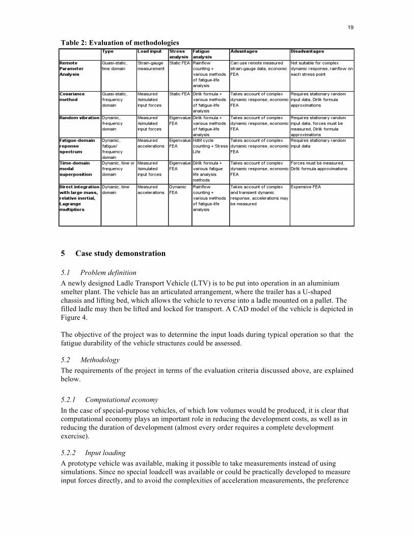
Table 2: Evaluation of methodologies

5 Case study demonstration

5.1 Problem definition A newly designed Ladle Transport Vehicle (LTV) is to be put into operation in an aluminium smelter plant. The vehicle has an articulated arrangement, where the trailer has a U-shaped chassis and lifting bed, which allows the vehicle to reverse into a ladle mounted on a pallet. The filled ladle may then be lifted and locked for transport. A CAD model of the vehicle is depicted in Figure 4. The objective of the project was to determine the input loads during typical operation so that the fatigue durability of the vehicle structures could be assessed.

5.2 Methodology The requirements of the project in terms of the evaluation criteria discussed above, are explained below.

5.2.1 Computational economy In the case of special-purpose vehicles, of which low volumes would be produced, it is clear that computational economy plays an important role in reducing the development costs, as well as in reducing the duration of development (almost every order requires a complete development exercise).

5.2.2 Input loading A prototype vehicle was available, making it possible to take measurements instead of using simulations. Since no special loadcell was available or could be practically developed to measure input forces directly, and to avoid the complexities of acceleration measurements, the preference

20

was to perform remote parameter strain-gauge measurements. The fact that vertical, lateral and longitudinal loads were expected to contribute, discouraged the use of the FESL methodology.

5.2.3 Higher-order dynamics The initial assumption was that higher-order dynamics would be excited on the vehicle frame.

5.2.4 Transient dynamic response The mission of the vehicle includes fixed routes through the plant and due to its stop-start nature, includes transient dynamic responses.

5.2.5 Accuracy of fatigue analysis For this type of design, fatigue failures can be expected, mainly at welded joints. These failures can be adequately dealt with by using design code SN-curves. Since it is a low-volume product, there would be no need for more complex methods to obtain greater accuracy, as appropriate safety factors may be applied.

5.2.6 Choice of methodology According to Figure 2 and Table 2, the methodology that fits the described requirements is Remote Parameter Analysis (described in paragraph 3.1 above). The following sections describe the application of this methodology to this project. As will become apparent, the choice of methodology had to be reconsidered during the execution of the project, owing to the unexpected results of measurement.

5.3 Measurements The following corresponds to the first step in paragraph 3.1. A number of strain-gauge transducers were applied to the LTV structure. The transducers used in the analyses were channels 3 and 4, which were near the front on top of the left and right chassis beams, sensitive to vertical bending stresses; channels 5 and 6, which were placed to the rear of the left and right chassis beams, sensitive to vertical bending stresses; as well as channels 7 and 8, which measured the bending stresses on the left and right vertical pillars. Measurements were taken during the typical operation of the prototype vehicle in the smelter plant.

5.4 Finite-element model and unit load analysis The following corresponds to the second and third steps in paragraph 3.1. A finite-element model of the vehicle structure was constructed. Static finite-element analyses of unit loads were performed using the finite-element model, calculating the stress response to 1 g of inertial vertical, longitudinal and lateral loading respectively.

5.5 Calculation of dynamic loads The following corresponds to the fourth step in paragraph 3.1. The purpose of the data from channels 3 and 4 was to derive the vertical and lateral loading. The vertical and lateral effects on these two channels were decoupled by adding them for vertical and subtracting them for lateral. This is depicted in Figure 5. The success of the decoupling can be observed by noticing that the lateral data excludes the effect of the ladle being lifted and put down, whereas the vertical data excludes the effect of turning.

21

Figure 4 Ladle Transport Vehicle (LTV)

Figure 5 Coupled and decoupled vertical and lateral channels

22

By also decoupling the data from channels 5 and 6 and then comparing the vertical data to the vertical data obtained from channels 3 and 4, it was found that they were mostly proportional to one another by a constant factor, which is the same factor determined from the finite-element model for pure vertical inertial loading, implying that the longitudinal loading was insignificant. A two-dimensional strain gauge / load transfer matrix [Kdecoupled] could therefore be composed from the finite-element results of the decoupled unit load:

Eq. 20 where σch3,1gvert is the finite-element stress result at the position of channel 3 for 1 g vertical loading, and similarly for the other components of the matrix. The dynamic vertical load, Vert_g(t), and lateral load, Lat_g(t), could then be calculated:

Eq. 21

5.6 Stress calculation The following corresponds to Step five in paragraph 3.1. The stress histories σ(t) at any position may then be calculated, using a critical. position / load transfer matrix [K]:

Eq. 22 Firstly, Eq. 22 is used to calculate the stresses at all strain gauge positions. Mathematically, this implies a perfect correspondence of this result with the measured stresses for channels 3 and 4, since these channels were employed to calculate the loads. It was found, however, that there was a poor correlation between the calculated stresses and the measured stresses, particularly at the pillar gauges (including channels 7 and 8), which prompted a reconsideration of the assumptions made previously.

23

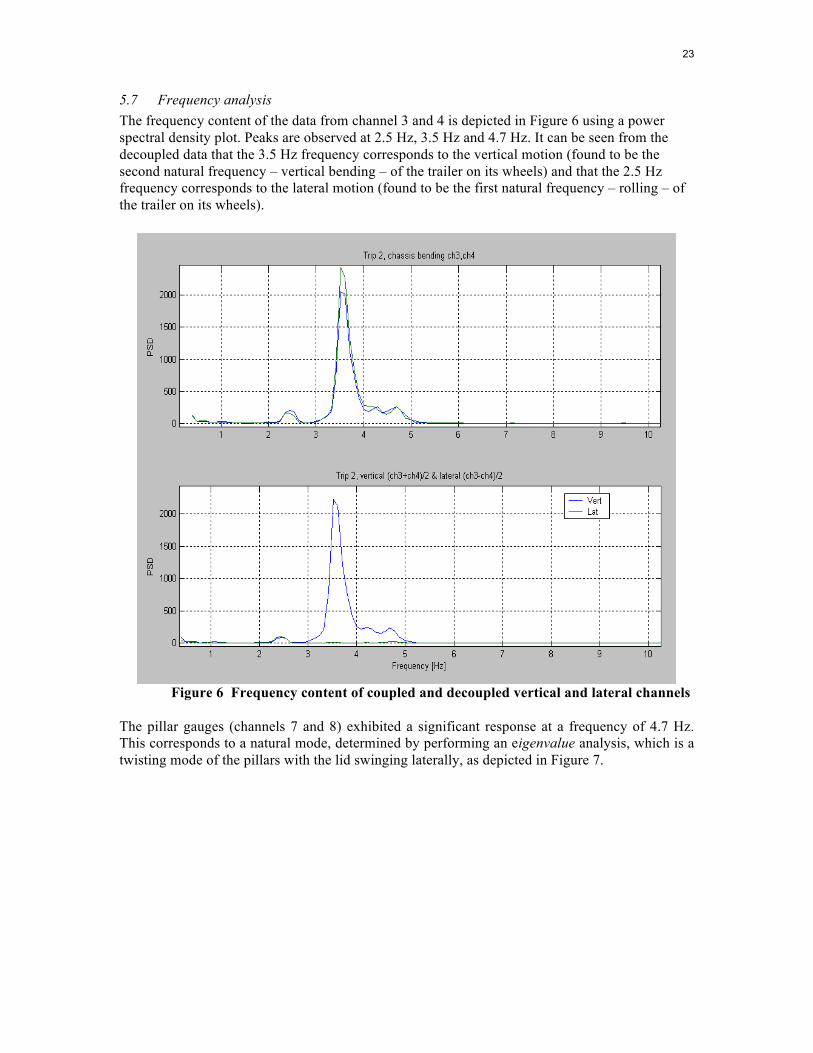
5.7 Frequency analysis The frequency content of the data from channel 3 and 4 is depicted in Figure 6 using a power spectral density plot. Peaks are observed at 2.5 Hz, 3.5 Hz and 4.7 Hz. It can be seen from the decoupled data that the 3.5 Hz frequency corresponds to the vertical motion (found to be the second natural frequency – vertical bending – of the trailer on its wheels) and that the 2.5 Hz frequency corresponds to the lateral motion (found to be the first natural frequency – rolling – of the trailer on its wheels).

Figure 6 Frequency content of coupled and decoupled vertical and lateral channels The pillar gauges (channels 7 and 8) exhibited a significant response at a frequency of 4.7 Hz. This corresponds to a natural mode, determined by performing an eigenvalue analysis, which is a twisting mode of the pillars with the lid swinging laterally, as depicted in Figure 7.

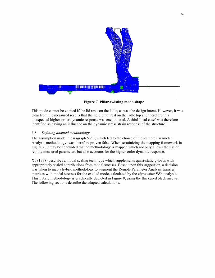
24

Figure 7 Pillar-twisting mode-shape

This mode cannot be excited if the lid rests on the ladle, as was the design intent. However, it was clear from the measured results that the lid did not rest on the ladle top and therefore this unexpected higher-order dynamic response was encountered. A third ‘load case’ was therefore identified as having an influence on the dynamic stress/strain response of the structure.

5.8 Defining adapted methodology The assumption made in paragraph 5.2.3, which led to the choice of the Remote Parameter Analysis methodology, was therefore proven false. When scrutinizing the mapping framework in Figure 2, it may be concluded that no methodology is mapped which not only allows the use of remote measured parameters but also accounts for the higher-order dynamic response. Xu (1998) describes a modal scaling technique which supplements quasi-static g-loads with appropriately scaled contributions from modal stresses. Based upon this suggestion, a decision was taken to map a hybrid methodology to augment the Remote Parameter Analysis transfer matrices with modal stresses for the excited mode, calculated by the eigenvalue FEA analysis. This hybrid methodology is graphically depicted in Figure 8, using the thickened black arrows. The following sections describe the adapted calculations.

25

Figure 8 Adapted methodology

Measurements Simulation

Quasi-static Dynamic STRESS ANALYSIS

LOAD INPUTS

FATIGUE ANALYSIS

Freq. domain Time domain Time domain

Multi-body dynamic simulation Unit load

Strain gauge / Load transfer matrix

L(t) Road profiles

a(t)

FFT/PSD

σ(t), ε(t)

Single dof response

Rainflow counting

Stress life FESL Strain life Fracture mechanics

Dirlik formula Material properties

FDRS curves

Static FEA

Transient dynamic direct integration

Eigenvalue FEA

Critical position / Load transfer matrix Modal

superposition

Large mass, relative inertial, or Lagrange multipliers

Covariance Method

26

5.9 Recalculation of dynamic loads In order to derive the vertical and lateral loads, the results of decoupled channels 3 and 4 were again used, together with the results of channel 7, used to solve for the modal contribution. The transfer matrix was therefore calculated as follows:

Eq. 23 The vertical and lateral g-loads, as well as the modal contribution, Modal(t), could therefore be solved as follows:

Eq. 24 The dynamic loads thus calculated were used as inputs into the critical position / load transfer matrix to calculate dynamic stress histories at all critical positions (including at all strain-gauge positions). A good correlation was found between the calculated and measured stress at redundant strain-gauge positions. Fatigue calculations, using rainflow-cycle counting and the stress-life criteria, completed the exercise.

6 Conclusion An overview was given of the existing methods and methodologies for the durability assessment of vehicle structures. These were mapped, using a common framework and compared for factors such as computational economy, requirements for input loading, as well as the incorporation of higher-order and transient dynamic responses. The framework offers a holistic view of the wide range of methods available for determining input loads and for performing stress analyses and fatigue analysis, but in sufficient detail to represent the integration of the methods into viable methodologies. The usefulness of the framework was demonstrated by its application to a case study.

27

7 References ASTM (American Society for Testing of Materials) E 1049-85. (1989). Standard practices for cycle counting in fatigue analysis. Bannantine, J.A., Comer, J.J. & Handrock, J.L. (1990). Fundamentals of metal fatigue analysis. Prentice-Hall. Bathe, K. (1996). Finite element procedures. Prentice Hall. Berger, C., Eulitz, K.-G., Heuler, P., Kotte, K.-L., Naundorf, H., Schuetz, W., Sonsino, C.M., Wimmer, A. and Zenner, H. (2002). Betriebsfestigkeit in Germany – an overview. International Journal of Fatigue, 24(6). Bishop, N.W.M. and Sherrat, F. (2000). Finite element based fatigue calculations. Glasgow: NAFEMS Ltd. Broek, D. (1989). The practical use of fracture mechanics. Dordrecht: Kluwer Academic Publishers. Captain, K.M., Boghani, A.B. & Wormley, D.M. (1979). Analytical tyre models for dynamic vehicle simulations. Vehicle system dynamics, 3. Chu, C.C. (1998). Multi-axial fatigue life prediction method in the ground vehicle industry. International Journal of Fatigue, 19(1). Conle, F.A., Chu, C.C. (1998). Fatigue analysis and the local stress-strain approach in complex vehicular structures, International Journal of Fatigue, 19(1). Dietz, S., Netter, H. & Sachau, D. (1998). Fatigue life prediction of a railway bogie under dynamic loads through simulation. Vehicle System Dynamics, 29. Dressler, K. and Kottgen, V.B. (1999). Synthesis of realistic loading specifications, European Journal of Mechanical Engineering, 41(3). European Convention for Constructional Steelwork (ECCS). (1985). Recommendations for the fatigue design of steel structures. Faria, L.O., Oden, J.T., Yavari, B., Tworzydlo, W.W., Bass J.M. & Becker, E.B. (1992). Tyre modelling by finite elements. Tyre Science Technology, 20. Fatemi, A. and Yang, L. (1998) Cumulative fatigue damage and life prediction theories: a survey of the state of the art for homogeneous materials. International Journal of Fatigue. Gopalakrishnan, R. & Agrawal, H.N. (1993). Durability analysis of full automotive body structures. Simulation and development in automotive simultaneous engineering, SAE SP-973. Grubisic, V. (1994). Determination of load spectra for design and testing, International Journal of Vehicle Design, 15(1). Gurney, T.R. (1976). Fatigue design rules for welded steel joints. The Welding Institute Research Bulletin, 17. Hobacher, A. (1996). Fatigue design of welded joints and components. International Institute of Welding. Huang, L., Agrawal, H.N. & Krurdiyara, P. (1998) Dynamic durability analysis of automotive structures. SAE Special Publications, v 1341, Advancements in Fatigue Research and Applications. Leever, R.C. (1983). Application of life prediction methods to as-welded steel structures. International Conference on Advances in Life Prediction Methods. ASME, New York. Miner, M.A. (1945). Cumulative damage in fatigue. Journal of Applied Mechanics, 12, Trans. ASME, 67. MSC Software Corporation. (1997). MSC/NASTRAN V70 Advanced Dynamics User’s Guide. Neuber, H. (1969). Anisotropic nonlinear stress-strain laws and yield conditions. International Journal of Solids & Structures, v 5, n 12. Olofsson, U., Svensson, T. & Torstensson, H. (1995). Response spectrum methods in tank-vehicle design, Experimental Mechanics , v 35, n 4. Oyan, C. (1998). Dynamic simulation of Taipei EMU train. Vehicle System Dynamics, 30. Pettersson, G. (2002). Fatigue analysis of a welded component based on different methods. Welding in the World, v 46, n 9/10.

28

Pountney, R.E. & Dakin, J.D. (1992). Integration of test and analysis for component durability. Environmental Engineering, 5(2). Recommendations for the Fatigue Design of Steel Structures. (1985). ECCS – Technical Committee 6 – Fatigue, Swiss Federal Institute of Technology, First Edition. Rixen, D.J. (2001). Generalized mode acceleration methods and modal truncation augmentation. Collection of Technical Papers - AIAA/ASME/ASCE/AHS/ASC Structures, Structural Dynamics and Materials Conference, v 2, p 884-894. Rui, Y., Borsos, R.S., Gopalakrishnan, R., Agrawal, H.N. & Rivard, C. (1993). The fatigue life prediction method for multi-spot-welded structures. Simulation and development in automotive simultaneous engineering, SAE SP-973. Rupp, A. (1989). Ermittlung von ertragbaren Schnittkraften fur die betriebsfeste Bemessung von Punktschweissverbindungen im Automobilbau. Forschungsvereinigung Automobiltechnik EV, 78. Ryu, J., Kim, H. & Wang, S. (1997). A method of improving dynamic stress computation for fatigue life prediction of vehicle structures. SAE 971534. Sherratt, F. (1996). Current applications of frequency domain fatigue life estimation, Environmental Engineering, 9(4). Society of Automotive Engineers Inc. (1997). SAE Fatigue Design Handbook AE-22. 3rd Edition. Warrendale, PA: SAE. Stephens, R.I., Dopker, B., Haug, E. J., Baek, W. K., Johnson, L. P. & Liu, T. S. (1987). Computational fatigue life prediction of welded and non-welded ground vehicle components. SAE 87967. Thomas, J.J., Nguyen-Tajan, T.M.L. & Burry, P. (2005). Structural durability in automotive design. Materialwissenschaft und Werkstofftechnik, 36(11). Wannenburg J. (1998). The applicability of static equivalent design criteria for the fatigue design of dynamically loaded structures. Proceedings of the Fifth International Colloquium on ageing of materials and methods for the assessment of lifetimes of engineering plant. Edited by Penny RK. Chameleon Press Ltd. Xu, H. (1998). An introduction of a modal scaling technique: an alternative and supplement to quasi-static g-loading technique with application in structural analysis. SAE 982810.