AN OVERVIEW OF DIFFERENT TURBULENCE MODELS APPLIED IN …

Proceedings of ENCIT 2012 14th Brazilian Congress of Thermal Sciences and Engineering

Copyright © 2012 by ABCM November 18-22, 2012, Rio de Janeiro, RJ, Brazil

AN OVERVIEW OF DIFFERENT TURBULENCE MODELS APPLIED IN A

FLOW WITHIN A 4-STAGES AXIAL-FLOW COMPRESSOR

Diego Thomas da Silva, [email protected] Technological Institute of Aeronautics, ITA – Gas Turbine Group

Jesuino Takachi Tomita, [email protected] Technological Institute of Aeronautics, ITA – Gas Turbine Group

Abstract. The flowfield calculation in axial flow turbomachines using CFD is not trivial, requiring special numerical

schemes and methods to reach the numerical convergence. One big issue in computational simulation, is the

mathematical representation of the turbulence effects, the turbulence modeling. The literature is scarced of detalied

studies about the influence of turbulence models in CFD simulation of multistage axial flow turbomachines. The

present investigation estimate the influence of four different turbulence models apllied in a flowfield determination of a

four-stage high pressure compressor (HPC). In this work, the well-known one-equation turbulence model, vastly

applied in aerodynamics, developed by Spalart and Allmaras, two equations standard k-ε model developed by Jones

amd Launder,the two equations k-ω model developed by Wilcox and largely used in aerospace aplications and the two

models developed by Menter, the two-equation model called SST and the seven equation model BSL Reynolds Stress

Modell were performed to compare its results in the case of a multistage axial compressor flow calculations. Fluid

properties contours, distribuitons and graphics were plotted. The differecences captured in flow proprierties were

concentrated in endwall regions and played a very important role which afected the prediction of turbomachinery

performance, flow patterns and compressor stall point.

Keywords: Turbomachinery, High Pressure Compressor, CFD, Turbulence Modeling, Gas Turbines

1. INTRODUCTION

During the early post II World War years, the gas turbine started to be manufacture at large scale for military and

civil purpose and researches were motivated by the Cold War. At that time, the compressors and turbines design

methodology was based on only in empirical correlations performed in many cascade tests. The data used in the

preliminary design came from tests using profiles as C4, C5, NACA series, DCA and MCA. At the 1950’s and 1960’s,

a large step occurred with the advance on computer science, hardware and starts the use of several numerical methods

as blade-to-blade and streamlines curvature as a common design tool (Horlock and Denton, 2005).

Currently, one and two-dimensional programs based on empirical correlations and the use of velocities triangles are

still in use during the preliminary design and its refinement to stacking the different airfoil sections from blade hub-to-

tip along its stages. Although these techniques provide good initial guesses of the turbomachines design configurations,

it is unable to supply detailed information about the flowfield characteristics within the turbomachine. At the moment, it

can be accomplished using experimental data or use of CFD techniques. During the machine development both

numerical and experimental procedures should be adopted (Smonly and Blaszczak, 1996). Numerical simulations tend

to decrease the development costs due to the reduction in the number of tests and its good fidelity of the results when

compared with test data. In this way, the CFD techniques are vastly used in several industrial projects including

turbomachines design.

About two decades ago, CFD codes were restricted to researches centers and large turbomachines industries, which

had high specialized teams to develop and validate the programs and resources using powerful computers. Commercial

software in many engineering areas were developed and are in use in industry by specialized groups in fluid mechanics,

heat transfer, thermodynamics and gas dynamics. Generally, these are user friendly, but needs high knowledge to use

and to analyze its results. However, there are many items and problems that need enhancements due to the complex

flow phenomena and numerical issues involved. (Denton, 2010) described several limitations behind the CFD applied in

turbomachines, much of them are not well understood. May be the cumbersome limitation is the incapability of CFD

calculation in evaluates correctly the losses, especially due the tip clearance flow responsible by almost one third of the

total losses.

These CFD errors are from mathematical simplifications of the physical phenomena and difficulties in the numerical

procedures to capture correctly all flow characteristics. It is consensus that the turbulence modeling is the more rude

simplification, where its effects are mathematically modeled due the incapability of the current computers to process the

amount of information needed if all the eddy scales were correctly captured. This type of simulation is called Direct

Numerical Simulation (DNS) and is restricted to simple cases only. Thus, a mathematical model to predict the effects of

the turbulence production, destruction, dissipation and vortices generations are need. The mathematical formulation

behind of the turbulent phenomena is complex, explaining the reasons of such few models are found in the literature for

each engineering problem.



The correct selection of the turbulence model is essential to provide correct results. When complex phenomena are

present as boundary layer separation, shock waves formation, heat transfer, and others, the difference between the

models become considerable, which requires a deeper study in turbulence modeling and its particularities and

limitations.

In this work an investigation in the use of two different turbulence models applied in a four-stage axial flow

compressor is performed. The motivation to perform the work is because the turbulence models are not general and a

single model is unable to supply accurate results for all turbomachine types and its particular characteristics (low,

moderate or high loading). The mass conservation, Navier-Stokes and energy conservation equations are calculated

using the Reynolds-Averaged Navier-Stokes (RANS) in the sense of finite-volume discretization technique. The

turbulence models chosen are the one-equation Spalart-Allmaras, the two equation models k-ε and k-ω, the BSL

Reynolds stress model and the SST. The results presents the capability of each turbulence model when it is used in a

high performance machine that have high pressure gradients involved within its flow domain.

2. NOMENCLATURE

BSL Base Line Reynolds Stress Model

CFD Computational Fluid Dynamic

HPC High Pressure Compressor

MUSCL Monotone Upstream-Centered Schemes for Conservation Laws

PR Total Pressure Ratio

RANS Reynolds-Averaged Navier-Stokes

SST Shear Stress Transport

LE Leading Edge

TE Trailing Edge

ηT Total-to-total Adiabatic Isentropic Efficiency

3. LITERATURE OVERVIEW

Many studies are found in literature comparing the results obtained using several turbutolence models in axial

turbomachnies, however, most of them are performed on static blades (Pecnik et al., 2005; Pasinato et al., 2004) or even

in cascades (Hjärne et al., 2007). Investigations over rotating blades are harder to be conducted despite the terms to

account the Coriolis and centripetal forces in momentum equations. One of the few studies performed and available is

the AGARD-AR-355 report (Dunham, 1998) where the flowfield through the NASA Rotor 37 was exhaustively

calculated by many different CFD codes and turbulence models. Other works were presented by different authors. It is

not rare to modifications in the models to correct the production or destruction of turbulence in different flows

(Elkhoury, 2007) or even to account the centripetal forces and high turning flows (Spalart e Shur, 1997)

In case of CFD simulation in multi-stage axial turbomachines, the computational procedures are not trivial,

demanding particular numerical schemes and its initialization schemes to start properly the numerical procedure.

(Denton, 1990) published a study describing a method to calculate viscous flows through multistage turbomachines,

given details about the mixing process between row interfaces. The author related special difficulties in reach the

solution in multistage axial compressors operating close the stall margin. According to the author, the transient part of

the calculation appears to conduct the component to enter in a stall operation, a numerical phenomenon, not physical.

To avoid this behavior, is essential to know very well the compressor operation envelop to ensure that each blade row is

operating close to the design point during the transient part of the calculation. A method to guarantee good numerical

stability in the firsts iterations is using a forcing mass-flow techniques and after a prescribed number of iterations these

forcing terms are turn-off.

Since this study of Denton, many others methods, algorithms and numerical schemes directed to turbomachines

simulations were presented. Nowadays, codes able to determinate the flowfield in axial turbomachines are

commercially available and their capabilities were proven in publication as (Mansour and Gunaraj, 2008) and (Belamri,

et al., 2005). Nonetheless, the technical literature lacks in studies about the turbulence modeling and its consequence in

multistage turbomachines and motivated the authors to conduct the present work.

4. METHODOLOGY

4.1 The Four-Stage HPC

The axial compressors are one of the most complex components to design to use in a gas turbine engine. Its

performance influences all the engine, a variation of 1% on compressors efficiency may reduce the SFC of the gas

turbine by 0.80% (Steinhardt, 2003). The HPC are even more complicated to develop, manufacture and determinate the

Proceedings of ENCIT 2012 Copyright © 2012 by ABCM

overall performance due the high speeds,

blade loading among other difficulties.

the pressure variation in each stage is higher, increasing the loading factor and flow diffusion causing the growth of

boundary-layer thickness and the possibility of its separation

1989). The shock wave is generally inevitable, but it is of

profiles to reduce the losses due to the shock

The present investigation was conducted with a 4

power with efficiency of 86% at 35,000 rpm. The mass flow

total pressure ratio of 4.41 (close to the stall line, for design

margin around 20%). The aspect ratio of the blades are

in stator blades. All these results is from the calculation based on the one

of blades per blade row follows above in

STAGE

Rotor Blades

Stator Blades

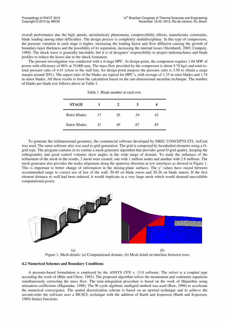
To generate the tridimensional geometry, the commercial software

was used. The same software also was used to

grid type. The program contains in its routine a mesh generator algorithm that provides good O

orthogonality and good control volumes skew angles

refinement of the mesh in the results, 2 mesh were created, one with 1 million nodes and another with 2.8 millions

mesh generator also provides the nodes alignment along the spanwise direction

This is important to better change of information in the mix

recommended range to correct use of law of the wall, 30

element distance to wall had been reduced, it would implicate in a very large mesh whi

computational power.

(a)

Figure 1. Mesh details: (a) Computational domain. (b)

4.2 Numerical Schemes and Boundary Condition

A pressure-based formulation is employed by the ANSYS CFX

according the work of (Rhie and Chow,

simultaneously correcting the mass flow.

relaxation coefficients (Majumdar, 1998)

the numerical convergence. The spatial discretization

second-order the software uses a MUSCL

1989) limiter functions.

14th Brazilian Congress of Thermal Sciences and Engineering

November 18-22, 2012, Rio de Janeiro, RJ, Brazil

overall performance due the high speeds, aeroelasticity phenomena, compressibility effects

. The design process is completely multidisciplinay. In th

variation in each stage is higher, increasing the loading factor and flow diffusion causing the growth of

layer thickness and the possibility of its separation, increasing the internal losses (Steinhardt

inevitable, but it is of designers’ responsibility to project turbomachines and blade

the shock formation.

s conducted with a 4-stage HPC. At design-point, the component

000 rpm. The mass flow provided by the compressor is about

(close to the stall line, for design-point purpose the pressure ratio is 3.50 to obtain a surge

ratio of the blades are typical for HPC’s, with average of 1.

from the calculation based on the one-dimensional meanline technique.

of blades per blade row follows above in Table 1.

Table 1. Blade number at each row.

STAGE 1 2 3 4

Blades 17 26 34 42

Blades 31 49 67 85

To generate the tridimensional geometry, the commercial software developed by NREC CONCEPTS ETI,

. The same software also was used to grid generation. The grid is composed by hexahedral elements using a O

The program contains in its routine a mesh generator algorithm that provides good O

rol volumes skew angles in the wide range of domain. To study the influence of the

refinement of the mesh in the results, 2 mesh were created, one with 1 million nodes and another with 2.8 millions

the nodes alignment along the spanwise direction at row interfaces

This is important to better change of information in the mixing-plane surfaces. The y+

values have stayed between

recommended range to correct use of law of the wall, 30-40 on blade rotors and 20-26 on blade stators. If the first

element distance to wall had been reduced, it would implicate in a very large mesh which would demand unavailable

(b)

(a) Computational domain. (b) Mesh detail on interface

and Boundary Conditions

based formulation is employed by the ANSYS CFX v. 13.0 software. The solver is a coupled type

, 1983). The proposed algorithm solves the momentum and continuity equations

mass flow. The time-integration procedure is based on the work of Majumbar

1998). The W-cycle algebraic multigrid method was used

e spatial discretization scheme is based on an upwind technique and t

MUSCL technique with the addition of Barth and Jesperson

Brazilian Congress of Thermal Sciences and Engineering 22, 2012, Rio de Janeiro, RJ, Brazil

, compressibility effects, manufacture constraints,

In this type of compressors,

variation in each stage is higher, increasing the loading factor and flow diffusion causing the growth of

(Steinhardt, 2003; Cumpsty,

responsibility to project turbomachines and blade

the component requires 1.04 MW of

is about 5.70 kg/s and total-to-

point purpose the pressure ratio is 3.50 to obtain a surge

33 in rotor blades and 1.74

dimensional meanline technique. The number

developed by NREC CONCEPTS ETI, AxCent

The grid is composed by hexahedral elements using a O-

The program contains in its routine a mesh generator algorithm that provides good O-grid quality, keeping the

domain. To study the influence of the

refinement of the mesh in the results, 2 mesh were created, one with 1 million nodes and another with 2.8 millions. The

at row interfaces as showed in Figure 1.

values have stayed between

26 on blade stators. If the first

ch would demand unavailable

interface between rows.

. The solver is a coupled type

he momentum and continuity equations

integration procedure is based on the work of Majumbar using

was used (Raw, 1996) to accelerate

scheme is based on an upwind technique and to achieve the

Jesperson (Barth and Jesperson,



The boundary conditions imposed in computational domain are:

• At inlet: total conditions (pressure and temperature), velocity vector angles and turbulence intensity;

• At outlet: static pressure with the application of radial equilibrium equation;

• At blade-to-blade surfaces: periodicity;

• At walls: non-slip condition;

• At inter-rows: mixing-plane approach.

4.3 Turbulence Models

Each turbulence model was developed for determined application, so there is no general model for all engineering

problems. Hence, the correct model selection is essential to obtain good results. If the aim of simulation of the flow

through a turbomachine is only to capture the average behavior of the flow, just a simple turbulence model might be

used (Casey, 2002). However, if complex characteristics are involved and should be determined, as secondary

phenomena or heat transfer rate, a more complete model is required including some numerical treatments.

It is important to avoid the use wall functions to determine the boundary-layer mainly in the flow with separations

(Röber et al., 2006) or when drag forces are important to be known. To accomplish that, a fine mesh and suitably

turbulence model is needed to capture properly the boundary layer. Sometimes, due the computational cost involved,

the user can not provide a suitably mesh to fully resolved the boundary layer correctly. In these cases, the user must be

able to generate a mesh size where the y+ values are in the range which the wall functions give satisfactory accuracy: 20

to 100 (Tsuei et al., 1999).

The ANSYS CFX v. 13.0 has a variety of turbulence models implemented in its routines, which enable the operator

tests as models as possible, searching for one that provide a good fit with the problem to be calculated. It is strongly

important that the user has familiarity with the whole mathematical formulation behind these models, its behavior and

limitations in each application. It is obtained just with experience and study in preview works. In view of this, five

models were chosen to simulate the flowfield in HPC with based on early papers and experience of the authors. The

chosen models are: k-ε, k-ω, SST, Spalart-Almaras and BSL.

The Standard k-ε model, developed by (Jones and Launder 1972) and recalibrated by (Launder and Sharma 1974),

is the most used and validated model in worldwide, being applied in many areas of engineering. The model solve one

equation for turbulent kinetic energy, k, and another for the turbulent dissipation, ε. The big drawback of this model is

its erroneous behavior close to the wall, which demands extremely low y+, in order of 0.2, and the use of dumping

functions close of the walls to keep the numerical stability. Because of that, normally the model are implemented with

wall function, which guarantee the numerical procedure robustness and the properly solution convergence, but its

prediction of boundary layer separation and flows under negative pressure gradient is, usually, inaccurate (Wilcox,

1998). Nevertheless, the k-ε, is still used due its numerical stability resulted of decades of studies and numerical

improvements in this model. Nowadays, there are different variations of this model (RNG and Realizable).

The k-ω model developed by Wilcox in 1980 decade was one of the pioneers in aerospace application. The model

solves one equation for turbulent kinetic energy, k, and another for turbulent dissipation rate, ω. According previews

studies, the model is very good to predict the flow inside of boundary layer but lacks in main flow due the high

turbulent production in freestream region (Menter, 1992). To overcome this shortcoming, Wilcox recommended in his

book (Wilcox 1998) a modification in two constants of the model, avoiding the overproduction of the turbulence in

absence of loss of prediction. In present work this modification was obeyed: the constants α and β0 were modified from

0.52 and 0.075 to 0.52 and 0.072, respectively.

Realizing the k-ω deficiency in main stream regions, (Menter, 1993) proposed in work (Menter, 1993) a new

model, the Shear Stress Transport (SST) that blends Wilcox model close the wall and k-ε in mainstream region was

developed. Adding on that, Menter modified the eddy-viscosity formulation to suppress the overproduction under

adverse pressure gradients flows. The author also created a turbulent kinetic limiter to avoid the overproduction in

stagnation regions, a known problem of two-equation turbulence models. The commercial package ANSYS CFX 13.0

use this limiter also in all two-equation models implemented in the program. The SST model has showing good

accuracy in turbomachienry flow calculation, predicting very well the boundary separation, secondary flows and

performance (Pecnik et al., 2005; Richardson, 2009).

The Spalart-Allmaras (SA) one equation model (Spalart and Allmaras 1992), is a model developed for flow over

aerodynamics profiles, but has been used in turbomachines successfully (Tartinville et al., 2007; Menter, 2003). Despite

the SA model is a one-equation model, it is a complete model that transports the modified eddy viscosity. The model

has also five terms to consider the transition effects, but it was not used in the preset work. The one equation model is

robust, providing very accurate results in axial turbomachines simulation (Santin, 2003; Tomita, 2009) at a low

computational cost which makes this model suitable during the design process (Menter, 2003).

The Reynolds Stress Models (RSM) is a different class of turbulence closures. Generally, these models solve 7

equations, one for each Reynolds tensor and one for dissipation or kinetic energy. These models are able to account the

effects of high streamline curvature naturally, without input a new source term. On the other hand, due the high

computational cost and time consuming in simulation, these models have been neglected during the design and analysis



procedure. With the improvement of computational power verified in the last decades, the simulation time was

meaningly reduced and scientists and engineers are looking again to these models seeking more accuracy in the

mathematical modeling of the turbulence. The ANSYS CFX 13.0 program has four different Reynolds Stress Models

implemented. Following literature recommendations, (Mansour and Gunaraj, 2008), and user's manual of the software,

the Baseline model (BSL) was chosen. The BSL mathematical formulation is also suggest by (Menter, 1993) and it is

similar of the SST, blending the k-ω and k-ε models, however without the new formulation of eddy viscosity. The

author chosen this model because is the only RSM model implemented in the program able to solve all the boundary

layer if the mesh is fine enough and provided good results in axial compressor (Mansour and Gunaraj, 2008).

5. Results

During the CFD solver start, the numerical stability is very poor, requiring some special attention. To start the

calculation, a dissipative scheme was used as a first-order discretization scheme for the Navier-Stokes equations (for the

convective terms) and a small outlet pressure. In case which the calculation procedure was started using a other

numerical order or higher outlet pressure, the numerical procedure diverged.

The first 250 numerical iterations were performed using the first-order scheme at 170 kPa of discharge pressure.

The procedure to reach the design point operation, was increase the outlet static pressure, in many steps increasing 30

kPa for each change, until the nominal pressure ratio at the same rotational speed. The numerical convergence was

monitored from the conserved variables residue, mass-flow and isentropic efficiency. The simulation was said

converged when the mass flow and the efficiency proved to be stable at a certain value. The variation of the inlet and

outlet mass was also checked, differences under 2% had been found in all simulations meaning the continuity equation

is converged.

The conserved variables residue presented poor convergence at mostly of the cases, except with k-ε and k-ω

turbulence models. For other turbulence models, the poor convergence can be associated with the Barth-Jesperson

limiter that was also verified and discussed by Venkatakrishman (Venkatakrishman, 1995) who proposed modification

in this high-resolution scheme to achieve the numerical convergence. However, Venkatakrishman also pointed that even

the residue did not reach the recommended value (in case of CFX program, values lower than 10-5

are recommended)

the numerical procedure can be assumed converged by monitoring other variables, in case of present work the mass

flow and efficiency.

Despite the design discharge pressure is 355 kPa, any simulation was able to reach this value at the compressor

outlet. The BSL model presented converged solution until the discharge pressure of 300 kPa, the smallest PR among the

models studied. Because of this poor numerical behavior of the BSL model, all the results comparison among the

models, were conducted at this outlet pressure.

The SA model performed little better, numerically speaking, and reached a discharge pressure of 310 kPa, as SST.

The both equation model, k-ε and k-ω showed the best performance providing converged solution at the least with

pressure discharge of 320 kPa because further pressure ratios were not tried.

The summary of results are addressed in the Table 2.

Table 2. Summary of results.

Turbulence Model PR Mass Flow(kg/s) ηT

k-ε 3,62 6,05 82,48

k-ω 3,65 6,19 83,15

SST 3,65 6,18 83,93

SA 3,58 5,83 80,41

BSL 3,6 5,94 82,46

It is notice that the SA results are the one which more differs from the other models with smaller PR, mass flow and

ηT.

The smaller mass flows predicted by the models compared from de design can be explained by the fact that the

simulation did not reach the design value. The same can be said about the isentropic efficiencies, which are

considerably smaller then the design.

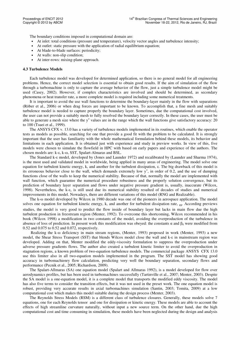
The Figure 2 brings the Mach number distribution along the meridional plane. About 60% of first rotor height is

choked for all cases. The k-ω and SST models predicted bigger supersonic region in the first rotor and higher velocities,

with sonic points in the second rotors. At the trailing edges hubs, the low velocities appear to be induced by the corner

separation. It is noticeable the in the second stator that the BSL predicted bigger region which is more remarkably. In

the others blade rows, the difference are not so strong.



Figure 2. Mach number distribution along the meridional plane.

Other difference is the Mach number contours in rotors are predicted slightly different at the tip. The SST and k-ω

models presented just slight differences at the tip, 1.297 and 1.296, respectively. The k-ε and BSL models predicted

small values at the tip, 1.287 and 1.283, respectively, and SA model obtained the highest speed, 1.304.

k-ε

k-ω

SST

SA

BSL



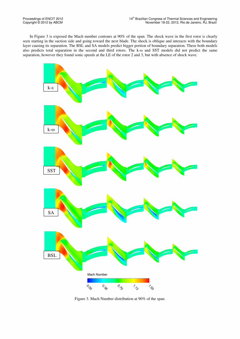
In Figure 3 is exposed the Mach number contours at 90% of the span. The shock wave in the first rotor is clearly

seen starting in the suction side and going toward the next blade. The shock is oblique and interacts with the boundary

layer causing its separation. The BSL and SA models predict bigger portion of boundary separation. These both models

also predicts total separation in the second and third rotors. The k-ω and SST models did not predict the same

separation, however they found sonic speeds at the LE of the rotor 2 and 3, but with absence of shock wave.

Figure 3. Mach Number distribution at 90% of the span.

k-ε

k-ω

SST

SA

BSL



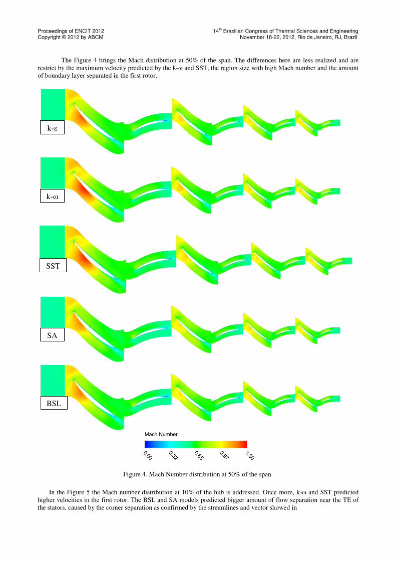
The Figure 4 brings the Mach distribution at 50% of the span. The differences here are less realized and are

restrict by the maximum velocity predicted by the k-ω and SST, the region size with high Mach number and the amount

of boundary layer separated in the first rotor.


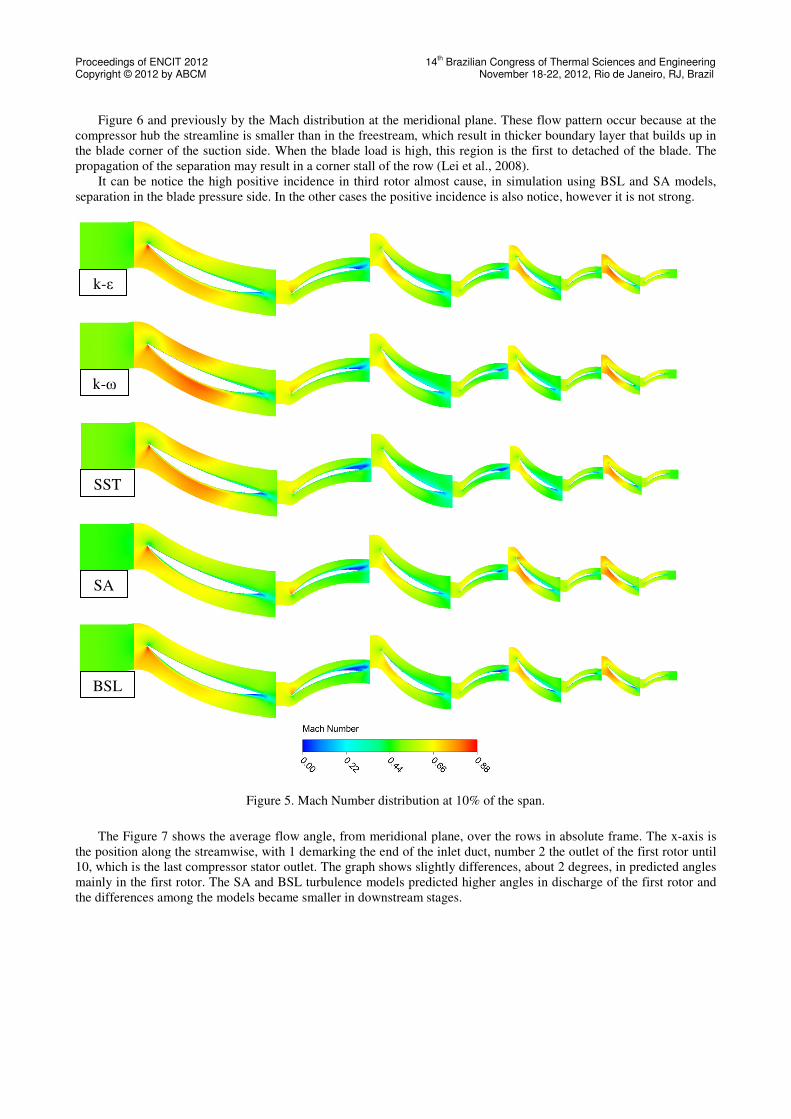
In the Figure 5 the Mach number distribution at 10% of the hub is addressed. Once more, k-ω and SST predicted

higher velocities in the first rotor. The BSL and SA models predicted bigger amount of flow separation near the TE of

the stators, caused by the corner separation as confirmed by the streamlines and vector showed in

k-ε

k-ω

SST

SA

BSL



Figure 6 and previously by the Mach distribution at the meridional plane. These flow pattern occur because at the

compressor hub the streamline is smaller than in the freestream, which result in thicker boundary layer that builds up in

the blade corner of the suction side. When the blade load is high, this region is the first to detached of the blade. The

propagation of the separation may result in a corner stall of the row (Lei et al., 2008).

It can be notice the high positive incidence in third rotor almost cause, in simulation using BSL and SA models,

separation in the blade pressure side. In the other cases the positive incidence is also notice, however it is not strong.


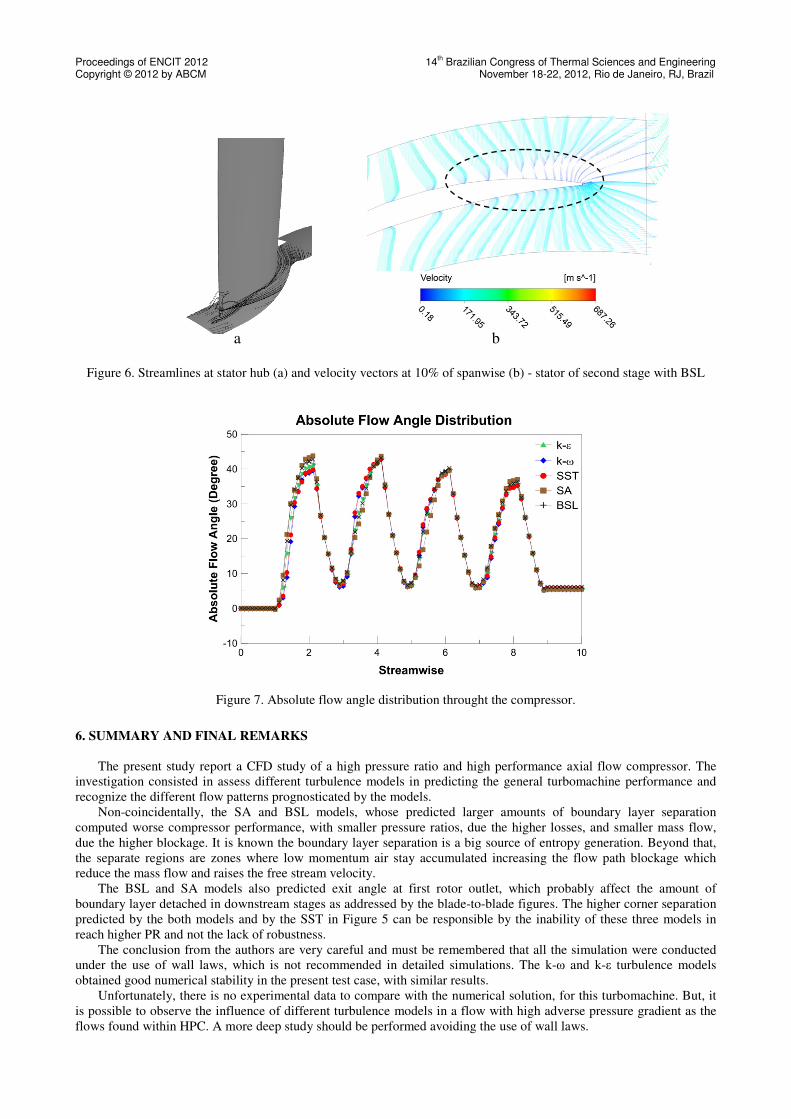
The Figure 7 shows the average flow angle, from meridional plane, over the rows in absolute frame. The x-axis is

the position along the streamwise, with 1 demarking the end of the inlet duct, number 2 the outlet of the first rotor until

10, which is the last compressor stator outlet. The graph shows slightly differences, about 2 degrees, in predicted angles

mainly in the first rotor. The SA and BSL turbulence models predicted higher angles in discharge of the first rotor and

the differences among the models became smaller in downstream stages.

k-ε

k-ω

SST

SA

BSL



Figure 6. Streamlines at stator hub (a) and velocity vectors at 10% of spanwise (b) - stator of second stage with BSL

Figure 7. Absolute flow angle distribution throught the compressor.

6. SUMMARY AND FINAL REMARKS

The present study report a CFD study of a high pressure ratio and high performance axial flow compressor. The

investigation consisted in assess different turbulence models in predicting the general turbomachine performance and

recognize the different flow patterns prognosticated by the models.

Non-coincidentally, the SA and BSL models, whose predicted larger amounts of boundary layer separation

computed worse compressor performance, with smaller pressure ratios, due the higher losses, and smaller mass flow,

due the higher blockage. It is known the boundary layer separation is a big source of entropy generation. Beyond that,

the separate regions are zones where low momentum air stay accumulated increasing the flow path blockage which

reduce the mass flow and raises the free stream velocity.

The BSL and SA models also predicted exit angle at first rotor outlet, which probably affect the amount of

boundary layer detached in downstream stages as addressed by the blade-to-blade figures. The higher corner separation

predicted by the both models and by the SST in Figure 5 can be responsible by the inability of these three models in

reach higher PR and not the lack of robustness.

The conclusion from the authors are very careful and must be remembered that all the simulation were conducted

under the use of wall laws, which is not recommended in detailed simulations. The k-ω and k-ε turbulence models

obtained good numerical stability in the present test case, with similar results.

Unfortunately, there is no experimental data to compare with the numerical solution, for this turbomachine. But, it

is possible to observe the influence of different turbulence models in a flow with high adverse pressure gradient as the

flows found within HPC. A more deep study should be performed avoiding the use of wall laws.

a b



7. ACKNOWLEDGEMENTS

The authors thank the Center for Reference on Gas Turbines at ITA for the support to this study.

8. BIBLIOGRAPHIC REFERENCES

Barth, T. J., and Jesperson, D. C., 1989. "The design and application of upwind schemes on unstructured mesehes".

AIAA Papes 89-0366.

Belamri, T., Galpin, P., Braune, A. and Cornelius, C., 2005. "CFD analysis of a 15 stage axial compressor part

I:methods". ASME TURBO EXPO 2005: Power for landing, sea and air.

Casey, M. V., 2002. "Validation of Turbulence Model for Turbomachinery Flows - A Review." Engineering Turbulence

Modelling and Experiments - 5, 43-57.

Cumpsty, N. A. , 1989. "Compressor aerodynamics". Krieger Publishing Company.

Denton, J. D. , 1990."The calculation of three dimensional viscous flow through multistage turbomachines".

Transactions of ASME (ASME-90-GT-19).

Denton, J. D., 2010. "Some Limitations of Turbomachinery CFD". ASME TURBO EXPO 2010: Power for landing, sea

and air.

Dunham, J., 1998."CFD Validation for Propulsion System Components". AGARD-AR-355, Neuilly-Sur-Seine.

Elkhoury, M., 2007."Assessment and Modification of One-Equation Models of Turbulence for Wall-Bounded Flows".

Journal of Fluids Engineering; Vol. 129, pp. 921-928.

Hjärne, J., Chernoray, V., Larson, J. and L. Löfdahl, 2007. "Numerical validations of secondary flows and loss

development downstream of a highly loaded low pressure turbine outlet guide vane cascade". ASME TURBO

EXPO 2007: Power for landing, sea and air.

Horlock, J. H., and Denton, J. D., 2005."A review of some early design practice using computational fluid dynamics

and current perspective". Journal of Turbomachinery 127, pp. 5-13.

Jones, W. P., and Launder, B. E., 1972. "The Prediction of Laminarization with a Two-Equation Model of Turbulence".

International Journal of Heat and Mass Transfer 15, No. 2, pp. 301-314.

Launder, B. E., and Sharma, B. I. 1974. "Appllication of the energy dissipation model of turbulence to the calculation of

flow near a spinning disc". Letters in Heat and Mass Transfer 1, No. 2 (1974), pp. 131-138.

Lei, V.-M, Spakovszky Z. S. and Greitzer E. M., 2008."A Criterion for Axial Compressor Hub-Corner Stall", Journal of

Turbomachinery, Vol. 130.

Majumdar, S., 1998. "Role underrelaxation on momentum interpolation for calculation of flow with nonstagarred

grids". Numerical Heat Transfer 13.

Mansour, M. L., and Gunaraj, J., 2008. "Validation of steady average-passage and mixing plane CFD approaches for

the performance prediction of a modern gas turbine multistage axial compressor". ASME TURBO EXPO 2008:

Power for landing, sea and air.

Menter, F. R., 1992. "Influence of Freestream Values on � − � Turbulence Model Predictions". AIAA Journal Vol. 30,

No. 6.

Menter, F. R., 2003."Turbulence modelling for turbomachinery". QNET-CFD Network Newsletter 2, No. 3.

Menter, R. F., 1993."Zonal Two-Equation k-w Turbulence Models for Aerodynamic Flows." 24th Fluid Dynamics

Conference, Orlando.

Pasinato, H. D., Squires, K. D. and Roy, R. P., 2004. "Assessment of Reynolds-averaged turbulence models for

prediction of the flow and heat transfer in an inlet vane-endwall passage". Journal of Fluids Engineering 126, pp.

305-315.

Pecnik, R., Pieringer, P. and Sanz, W., 2005. "Numerical investigation of the secondary flow of a transonic turbine

stage using various turbulence models." ASME TURBO EXPO 2008: Power for landing, sea and air, Reno-Tahoe.

Raw, M. J., 1996. "Robustness of coupled algebric multigrid for the Navier-Stokes equations", AIAA 34th Aerospace

Sciences Meeting and Exhibit, Reno.

Rhie, C. M., and Chow, W. L., 1983. "Numerical study of the turbulent flow past an isolated airfoil with the trailing

edge separation". AIAA Journal, Vol. 21, No. 11, pp. 1525-1532.

Richardson D., 2009. "Unsteady Aerodynamics of High Works Turbines". Engineering Doctorate Thesis, Cranfield,

England.

Röber, T., Kozulovié, D. , Kügeler, E. and D. Nürnberger, 2006."Appropriate turbulence modelling for turbomachinery

flows using a two-equation turbulence model". Notes on Numerical Fluid Mechanics and Multidisciplinary Design

92/2006 pp. 446-454.

Santin M. A. B., 2006. Simulação Numérica de Escoamento em Turbinas de Alto desempenho. Master's Thesis,

Instituto Tecnológico de Aeronáutica, São José dos Campos, SP, Brazil.

Smonly, A., and Blaszczak, J., 1996."Boundary layer and loss study in highly loaded turbine cascade". AGARD-CP-

571, Neuilly-Sur-Seine.



Spalart, P. R., and Allmaras, S. S., 1992. "A One-Equation Turbulence Model for Aerodynamic Flow". AIAA 30th

Aerospace Sciences Meeting and Exhibit, Reno.

Spalart, P. R., and Shur, M., 1997. "On the Sensitization of Turbulence Models to Rotation and Curvature". Aerospace

Science and Technology, n 5, pp. 297-302.

Steinhardt, E., 2003. "HP compressor design". von Karman Institute: Lecture series 2003-06.

Tartinville, B., Lorrain, E. and Hirsch, C., 2007."Application of the v²-f turbulence model to turbomachinery

configurations". ASME TURBO EXPO 2007:Power for landing, sea and air.

Tomita J., T., 2009. " Three-Dimensional Flow Calculations of Axial Compressors and Turbines Using CFD

Techniques. Ph.D. Thesis, Instituto Tecnológico de Aeronáutica, São José dos Campos, SP, Brazil.

Tsuei, H. -H., Oliphant, K. and Japiske, D., 1999. "The validation of rapid CFD modeling for turbomachinery." CFD

Technical Developments and Future Trends, London.

Venkatakrishman, V., 1995. "Convergence to steady state solutions of the Euler equations on unstructured grids with

limiters", Journal of Computational Physics, pp. 120-130.

Wilcox D. C., 1998. "Turbulence Modelling for CFD". DCW Industries, Second Edition. La Canãda.

9. RESPONSIBILITY NOTICE

The authors are the only responsible for the printed material included in this paper.

Documents

AN OVERVIEW OF DIFFERENT TURBULENCE MODELS APPLIED IN …