Embed Size (px)
Citation preview
int j prod res 1999 vol 37 no 17 3859plusmn 3881
An overview of design and operational issues of kanban systems
M S AKTURK and F ERHUN
We present a literature review and classireg cation of techniques to determine boththe design parameters and kanban sequences for just-in-time manufacturingsystems We summarize the model structures decision variables performancemeasures and assumptions in a tabular format It is important to state thatthere is a signireg cant relationship between the design parameters such as thenumber of kanbans and kanban sizes and the scheduling decisions in a multi-item multi-stage multi-horizon kanban system An experimental design is devel-oped to evaluate the impact of operational issues such as sequencing rules andactual lead times on the design parameters
1 Introduction
In recent years the term just-in-time (JIT) has become a common term inrepetitive manufacturing It is used to describe a management philosophy thatencourages change and improvement through inventory reduction JIT can bedereg ned as the ideal of having the necessary amount of material available where itis needed and when it is needed It is an attempt to produce items in the smallestpossible quantities with minimal waste of human and natural resources and onlywhen they are needed JIT systems have proven to be e ective at meeting productiongoals in environments with high process reliability low setup times and low demandvariability (Groenevelt 1993) In general JIT has a pull system of coordinationbetween stages of production In a pull system a production activity at a stage isinitiated to replace a part used by the succeeding stage whereas in a push systemproduction takes place for future need
The advantages of JIT production include reduced inventories reduced leadtimes higher quality reduced scrap and rework rates ability to keep schedulesincreased macr exibility easier automation and better utilization of workers and equip-ment However there is a limit to the extent that JIT can be usefully applied in manyindustries The major JIT successes are in repetitive manufacturing environments Ifthe demand cannot be predicted accurately and product variety cannot be con-strained it may not be possible to implement JIT e ectively The reg nal assemblyschedule must also be very level and stable In pull approaches information macr owis tied to material macr ow hence valuable information (e g on the demand trend) is notsent to all stages of production as soon as it is available Pull systems can therefore
International Journal of Production Research ISSN 0020plusmn 7543 printISSN 1366plusmn 588X online 1999 Taylor amp Francis LtdhttpwwwtandfcoukJNLSprshtm
httpwwwtaylorandfranciscomJNLSprshtm
Revision received August 1998 Department of Industrial Engineering Bilkent University 06533 Bilkent Ankara
TurkeyTo whom correspondence should be addressed e-mail akturkbilkentedutr
be characterized by large information lead times especially where there are largematerial macr ow times
One of the major elements of JIT philosophy and pull mechanism is the kanbansystem Kanban is the Japanese word for visual record or card In a kanban systemcards are used to authorize production or transportation of a given amount ofmaterial This system is the information processing and hence shop-macr oor controlsystem of JIT philosophy While kanbans are being used to pull the parts they arealso used to visualize and control in-process inventories The system e ectively limitsthe amount of in-process inventories and it coordinates production and transporta-tion of consecutive stages of production in assembly-like fashion Therefore akanban system is the manual method of harmoniously controlling production andinventory quantities within the plant The kanban system appears to be best suitedfor discrete part production feeding an assembly line
Kanban system can be either dual-card or single-card The dual-card kanbansystem employs two types of kanban cards production kanban and transportation(also called conveyance or withdrawal) kanban A transportation kanban dereg nes thequantity that the succeeding stage should withdraw from the preceding stage Aproduction kanban on the other hand dereg nes the quantity of the specireg c partthat the producing stage should manufacture in order to replace those which havebeen removed (Groenevelt 1993) Even though the dual-card kanban system pro-vides strong control on the production system due to its strict assumptions andprerequisites such as design of the manufacturing system smoothing of productionand standardization of operations it is di cult to implement it Therefore a variantof this system called single-card kanban system is sometimes used as a reg rst stage todevelop a dual-card kanban system In single-card kanban system the transporta-tion of materials is still controlled by transportation kanbans However a produc-tion schedule provided by the central production planning is used to control theproduction within a cell instead of the production kanbans Hence the system has astrong similarity to a conventional push system with pull elements added to coor-dinate the transportation of the parts One of the advantages of single-card push-pullsystem is its simplicity in implementation Moreover as the information on demandtrend is sent to all stages of production as soon as its available single-card kanbansystem has shorter information lead times compared to dual-card kanban systemsOn the other hand single-card kanban systems can also be used when the succeedingstage is physically close to its predecessor In this case the transportation kanban iseliminated and containers are moved at a time as needed Only production kanbansare used In this study we use the former dereg nition of a single-card kanban systemwhere the transportation of materials between the di erent workcentres is controlledby transportation kanbans
Kanban system can be either instantaneous or periodic review system In instan-taneous review systems the kanbans are dispatched upstream as soon as an orderoccurs In periodic review systems the kanbans are collected and dispatched per-iodically Periodic review systems may be either reg xed quantity non-constant with-drawal cycle or reg xed withdrawal cycle non-constant quantity (Monden 1993)Under the reg xed quantity non-constant withdrawal cycle system kanbans are dis-patched upstream when the number of kanbans posted on a withdrawal kanban postreaches a predetermined order point Under the reg xed withdrawal cycle non-constantquantity system the period between material handling operations is reg xed and thequantity ordered depends on the usage over the withdrawal cycle
3860 M S Akturk and F Erhun
2 Literature review
We reg rst provide a comparative review of kanban literature on determining thedesign parameters using a tabular format then discuss the studies on determining thekanban sequences to show the impact of operational issues on the design parameters
21 Determining the design parametersIn this section we review the models for determining the design parameters in a
kanban system and summarize the model structures decision variables perform-ance measures and assumptions in a tabular format The characteristics consideredin this review are classireg ed as follows (the emboldened letters give the key to theentries in table 1 later)
1 Model structure Mathematical programming Simulation Markov ChainsOthers
2 Solution approach
21 Heuristic22 Exact Dynamic programming Integer programming Linear program-
ming Mixed integer programming Nonlinear integer programming3 Decision variables
31 Number of kanbans32 Order interval33 Safety stock level34 Kanban size
4 Performance measures
41 Number of kanbans42 Utilization43 Measures Inventory holding cost Shortage cost Fill rate
5 Objective
51 Minimize cost Inventory Holding cost Operating costs Shortage costSeTup cost
52 Minimize inventory53 Maximize throughput
6 Setting
61 Layout Assembly-tree Serial Network without backtracking62 Time period Multi-periodSingle-period63 Item Multi-item Single-item64 Stage Multi-stage Single-stage65 Capacity Capacitated Uncapacitated
7 Kanban type Single-card kanban Dual-card kanban8 Assumptions
81 Kanban sizes Known Unit82 Stochasticity Demand Lead time Processing time Setup time83 Production cycle Fixed production intervals Continuous production84 Material handling Fixed withdrawal cycle Instantaneous85 No shortages86 System Reliability Dynamic demand Machine unreliability Imbalance
between stages Rework
3861Overview of kanban systems
Most of the existing studies in the literature are modelled by using a mathemat-ical programming Markov chain or simulation approaches There are a few excep-tional studies that use other methods such as statistical analysis or the Toyotaformula In table 1 later we collect these models under the heading othersrsquo Onthe other hand a solution approach can be either heuristic or exact For an exactsolution methodology one of the dynamic programming integer programminglinear programming mixed integer programming or nonlinear integer programmingtechniques can be used to reg nd an optimum solution
For the analytical models the decision variables are mainly kanban sizes numberof kanbans withdrawal cycle length for periodic review models and safety stocklevels For the simulation models the commonly used performance measures arenumber of kanbans machine utilizations inventory holding cost backorder costand reg ll rates Fill rate can be dereg ned as the probability that an order will be satisreg edthrough inventory Models can consider di erent combinations of the criteria statedabove The objectives for the analytical models can be minimizing the costs orminimizing the inventories For the cost minimization the cost terms can be con-sidered either independently as inventory holding cost shortage cost and setup costor the combination of these costs as an operating cost Another objective for stoch-astic models can be maximizing the throughput of the system
The production setting for the models include the layout number of time peri-ods number of items number of stages and capacity Layout can be serial (macr ow-line) assembly-tree or a general network without backtracking (modireg ed macr owline)An empty cell in the table for any of these indicate that the characteristic is notconsidered in the corresponding study
Kanban system can be either a single-card or a dual-card The assumptions forthe models are also stated in the tabular format These assumptions are the ones thatare commonly considered more specireg c ones are indicated in the explanations of themodels The reg rst assumption is on the kanban size An empty cell for this character-istic indicates that the kanban size is not a parameter but is a decision variable forthe system Another assumption relates to the nature of the system such that thesystem can be either stochastic or deterministic For the deterministic models thiscell is left empty For the stochastic ones the stochastic parameters are indicatedThe production cycle di erentiates between the models that have continuous pro-duction and reg xed production intervals The fourth assumption specireg es the materialhandling mechanism and it can be either an instantaneous or a periodic one Thereg fth assumption is related to backorders An empty cell indicates that backorder isallowed And the last assumption is on the system reliability If the system is re-liable this cell is left empty otherwise the unreliability of the system is stated Intable 1 the models are presented using the classireg cation scheme listed at the start ofsect 21 Further explanations of the models are given below
Kimura and Terada (1981) describe the operation of kanban systems and ex-amine the accompanying inventory macr uctuations in a JIT environment They provideseveral balance equations for kanban systems in a single item multi-stage uncapa-citated serial production setting to demonstrate how demand macr uctuations of the reg nalproduct inmacr uence the macr uctuations of production and inventory at the upstreamstages The authors use simulation to show that macr uctuations are amplireg ed whenthe size of order andor lead time becomes large
Huang et al (1983) simulate the JIT with kanban for a multi-line multi-stageproduction system in order to determine its adaptability to a US production envir-
3862 M S Akturk and F Erhun
3863Overview of kanban systems
Kim
ura
ampTe
rad
a
Hu
ang
et a
l
Bitr
anamp
Ch
an
g
Ree
s e
t al
Miy
aza
ki e
t al
Gu
pta
ampG
upta
Ka
rma
rka
rampK
ekr
e
Phili
po
om
et a
l
Wa
ng
ampW
ang
Mitr
aamp
Mitr
ani
Year 81 83 87 87 88 89 89 90 90 90Model Structure MS S M O O S C MS C CS
Solution HeuristicA pproach D I L M N NM I
of kanbans X X X X X X XDecision order interval XVariables safety stock
kanban size X XPerformance of kanbans
Measures utilization XI S F I IScost O O HS HST HS HST HS
Objective inventory Xthroughput X
layout S A A A N Shorizon M M M M S S S M
Setting item S M S S S M M Mstage M M M M M M M M
capacity U C C C C U UKanban Type S D D D D D D D SD D D S
kanban size K K K U K K Kstochasticity D DP L P DP D DP
Assumptions production cycle F C F C F C F F C Cmaterial handling I I I I F I I F I I
no shortages X Xsystem reliability I D MI M
Ba
rdamp
Go
lon
y
Liamp
Co
Mitt
alamp
Wa
ng
Ask
in e
t a
l
Mitw
asi
ampA
skin
Tak
ah
ash
i
Oh
no
et
al
Phili
po
om
et
al
Be
rkle
y
Mo
ee
ni e
t a
l
Y ear 91 91 92 93 94 94 95 96 96 97Model Structure M M S C M S O M S OS
Solution Heuristic XA pproach D I L M N M D NM I
of kanbans X X X X X XDecision order intervalV ariables safety stock X X
kanban size XPerformance of kanbans X X
Measures uti lizationI S F IF IFcost SH ST H HS O HSST HST
Objective inventorythroughput
layout A SA N S S A S Shorizon M M M S M M M M M M
Setting item M S M M M S S M M Sstage M M M M S M S M M M
capacity C U C C C CKanban Type S D S D D S D D D D D S
kanban size K K K K K K U Kstochasticity DP DP DP D DP D PS
A ssumptions production cycle F F F F C F F C Fmaterial handling I I I I I I I I I I
no shortages X X Xsystem reliability MR D I M
Table 1 Models for kanban systems choosing design parameters (see text for key)
onment The simulated production system includes variable processing times (nor-mally distributed) variable master production scheduling (exponentially distributeddemand) and imbalances between production stages The authors conclude that thevariability in processing times and demand rates are amplireg ed in a multi-stage set-ting and that excess capacity has to be available to avoid bottlenecks Monden(1984) comments on the conclusion drawn by Huang et al (1983) He stated thatthe kanban system should be able to adapt to daily changes in demand within 10deviations from the monthly master production schedule (MPS) Larger seasonalmacr uctuations in demand can be accommodated by setting up the monthly MPSappropriately
Bitran and Chang (1987) extend Kimura and Teradarsquos (1981) serial model Theyprovide a nonlinear integer formulation for kanban systems in a deterministic singleitem multi-stage capacitated assembly-tree structure production setting The for-mulation assumes zero transportation lead time and planning periods of knownlength and reg nds the minimum feasible number of kanbans The authors showthat the initial nonlinear model can be transformed into an integer linear programwith the same feasible and optimal solutions The proposed model does not incor-porate uncertainties
Rees et al (1987) develop a methodology for dynamically adjusting the numberof kanbans in an unstable production environment They use the Toyota equationwith unit kanban capacities forecasted demands and estimates of kanban lead timeprobability density functions to determine the number of kanbans
Miyazaki et al (1988) modify the conventional economic order quantity model todetermine the average inventory for reg xed interval withdrawal and supplier kanbansystems give formulae to determine the minimum number of kanbans required andderive an algorithm to obtain the optimal order interval The objective is to minimizethe average inventory holding and ordering costs in a deterministic setting
Gupta and Gupta (1989) simulate a single item multi-line multi-stage dual-cardkanban system They investigate the impact of changing the number of kanbans andkanban sizes on the performance of the system The performance measures arechosen to be in-process inventory capacity utilization or production idle time andshortage of the reg nal product The authors conclude that determining the number ofkanbans is essential to the performance of the system and keeping the bu er sizeconstant by increasing the kanban size and decreasing the number of kanbansaccordingly increase the inventory For the smooth operation in a JIT environmentthe stages should be balanced and the suppliers should be reliable Finally thesystem performance declines with an increase in demand variability
Karmarkar and Kekre (1989) develop a continuous time Markov model to studythe e ect of batch sizing policy on production lead time and inventory levels Bothsingle and dual card kanban cells and two-stage systems are modelled They alsoexamine the e ect of varying the number of kanbans in the cell The primary intentof the investigation is to develop a qualitative analysis of kanban systems that canprovide insights to parametric behavior of kanban systems The results show that thekanban size has a signireg cant e ect on the performance of kanban systems
Philipoom et al (1990) describe the signal kanban technique and demonstratetwo versions of an integer mathematical programming approach for determining theoptimal lot sizes to signal kanbans in a multi-item multi-stage setting A simulationmodel is employed to test the e ectiveness of the programming models The models
3864 M S Akturk and F Erhun
assume no backorders therefore the stages are decoupled and interdependencies areeliminated
Wang and Wang (1990) present a continuous time Markov model to determinethe number of kanbans in a multi-item multi-stage dual-card kanban system with asingle withdrawal kanban for each stage The model can be applied to serial as-sembly (merge) type and disassembly (split) type production settings The authorsassume that the production and demand rates are exponential Furthermore thestages are assumed to be independent To determine the number of kanbans severalalternatives for number of kanbans are considered and the one with minimum costis chosen The model can be extended to systems with unreliable machines
Mitra and Mitrani (1990) present a continuous time Markov model for a multi-item multi-stage serial production setting The processing times are exponentiallydistributed and the raw material and demand arrival have Poisson distribution Theauthors show the equivalence of kanban system to the tandem sequence with mini-mal blocking policy They also show that under their distribution assumptions thethroughput-inventory relation of kanban system dominates that of traditional dis-cipline of manufacturing blocking The authors develop an approximation algor-ithm which is compared with a simulation model As a result they observe that theapproximation has the largest errors in the long production lines with few kanbancards in each cell The model can be extended to systems with unreliable machines
Bard and Golony (1991) develop a mixed integer linear program to determine thenumber of kanbans at each stage in a multi-item multi-stage capacitated generalassembly shop The objective is to minimize inventory holding shortage and setupcosts for a given demand and planning horizon without violating the basic kanbanprinciples The model is most appropriate when the demand is steady and the leadtimes are short
Li and Co (1991) extend Bitran and Changrsquos (1987) model to develop bounds foran e cient kanban assignment and apply them to solve a dynamic programmingmodel in a deterministic single item multi-stage serialassembly-tree structure pro-duction setting The authors assume an inreg nite capacity This assumption not onlyremoves the capacity constraints but also eliminates the need to keep track of thenumber of units in partially reg lled kanbans Therefore the model is computationallyvery e cient even for a complex non-serial system
Mittal and Wang (1992) develop a database-oriented simulator called CADOK(computer aided determination of kanbans) to determine the number of kanbans ina production setting where breakdowns reworks setup times variable processingtimes (normally distributed) and variable demand (exponentially distributed) aremodelled Backorder costs are assumed to be prohibitively high The model canhandle both assembly and disassembly type operations such that several stagessupply products to the same stage or one stage supplies parts to several stagesFurthermore delay can be induced for the information to travel from one stage toanother However the system cannot handle backtracking so it is only applicable tomacr owlines or modireg ed macr owlines
Askin et al (1993) develop a continuous time steady-state Markov model fordetermining the optimal number of production kanbans in a multi-item multi-stageserial production setting The objective is to minimize the inventory holding andshortage costs given external demand and the kanban sizes The external demandassumption permits the modelling of a multi-stage system as independent stages Themodel uses the Toyota equation and reg nds the number of kanbans and safety factor
3865Overview of kanban systems
The performance of the model is sensitive to the accurate estimation of the queuelengths
Mitwasi and Askin (1994) provide a nonlinear integer mathematical model forthe multi-item single stage capacitated kanban system It is assumed that demand isexternal dynamic and evenly distributed over period the system is reliable setupsare small enough to allow batch sizes as small as a single kanban and no shortagesare permissible The control periods are assumed to be small enough to ignore batchsequencing problem The model is transformed to a simpler model with the same setof optimal and feasible kanban solutions Lower and upper bounds for the numberof kanbans are developed A heuristic solution is also presented
Takahashi (1994) provides a simulation model to determine the number ofkanbans for a single item unbalanced serial production systems under stochasticconditions (demand with exponential distribution and processing time with gammadistribution) An algorithm that allows di erent numbers of production and with-drawal kanbans at an inventory point is proposed It is assumed that the totalnumber of kanbans are known withdrawal lead time is negligible and backordersare allowed
Ohno et al (1995) derive the stability condition of a JIT production system withthe production and supplier kanbans under the stochastic demand and deterministicprocessing times An algorithm for determining the optimal number of two kinds ofkanbans that minimize an expected average cost per period is devised In otherwords this algorithm determines the optimal safety stocks in the Toyota equation
Philipoom et al (1996) provide a nonlinear integer mathematical model for themulti-item multi-stage multi-period capacitated kanban system It is assumed thatdemand is deterministic the system is reliable setups are sequence-independentproduction costs are stable lot sizes remain constant throughout the shop and noshortages are permissible The model determines the kanban sizes number of kan-bans and reg nal assembly sequence simultaneously by minimizing the setup andinventory holding costs
Berkley (1996) investigates the e ect of kanban size on system performance in amulti-item multi-stage dual-card kanban system The performance measures are in-process inventory and customer service level The author varies the number of kan-bans and kanban sizes in the tandem so that the total in-process inventory capacityremains constant Simulation results show that smaller kanban sizes lead to smallerin-process inventories and smaller kanban sizes can lead to better customer servicewhen the cost of the greater setup times can be o set by the benereg ts of more frequentmaterial handling The study assumes that the kanban sizes and number of kanbansare same for all parts and the set of kanban size values are independent of thedemand distribution
Moeeni et al (1997) propose a methodology based on Taguchirsquos robust designframework to implement kanban systems in uncertain production environmentsThe authors model the e ects of environmental variations such as demand patternssupplier lead times setup times processing times time between breakdowns andrepair times on the kanban system performance To evaluate the performance ofdesign they use a quadratic loss function The proposed methodology is examinedvia simulation An experimental design that considers the number of kanbanskanban review periods and container sizes simultaneously is performed The authorsreg nd that for their system the container size is the most important factor in terms ofthe performance measures used
3866 M S Akturk and F Erhun
The current literature can be extended in several ways For each part in theKanban system two basic design parameters have to be determined the kanbansize and the number of kanbans to be used Very few studies exist that considerthe kanban sizes explicitly ie Gupta and Gupta (1989) Karmarkar and Kekre(1989) Philipoom et al (1996) and Moeeni et al (1997) Berkley (1996) studiesthe e ect of kanban sizes on system performance but he assumes that the kanbansizes are set regardless of the demand distribution Most of the models assume thatthe kanban sizes are known and the number of kanbans can be determined by usingthese predetermined values In fact the number of kanbans and kanban sizes shouldbe determined simultaneously as these two together a ect the performance of thesystem Almost none of the models except Philipoom et al (1996) considerthe impact of operating issues on design parameters It is usually assumed that thecontrol periods are small enough to ignore the batch sequencing problem Even inthe study of Philipoom et al only the reg nal assembly sequence is determined and it isassumed that it propagates back by the reg rst-come-reg rst-served (FCFS) rule In gen-eral instantaneous material handling is used There are only two models that usenon-instantaneous material handling by Miyazaki et al (1988) for supplier andwithdrawal kanbans and by Philipoom et al (1990) for signal kanbans Themodel structures are di erent and their reg ndings cannot be generalized to a dual-card kanban system
Several models in the literature assume station independence Askin et al (1993)and Mitwasi and Askin (1994) assume external demand The demand for each stageis externally generated and with the assumption of su cient capacity the multi-stagesystem can be modelled as independent stages linked by their proportional demandrates Kimura and Terada (1981) Philipoom et al (1990) and Li and Co (1991)assume that the capacity is unlimited Bitran and Chang (1987) Philipoom et al(1990) and Philipoom et al (1996) do not allow backorders Under JIT system allstages are integrally tied to each other and if there is a delay in one stage then boththe preceding and succeeding stages should be a ected to highlight interdependenciesamong the stages This is crucial for reducing the size of the inventory levels andeliminating overall waste Although this possibility is eliminated with the assumptionof no backorders and an inreg nite production capacity hence each stage can bemodelled independently
22 Determining the kanban sequencesIn JIT systems the reg nal assembly schedule determines production orders for all
of the stages in the facility Once the assembly line is scheduled it is assumed that thesequence propagates back through the system Kanbans in the rest of the shop areprocessed in order in which they are received ie FCFS However there are severalstudies in the literature that test this assumption
Lee (1987) compares the FCFS shortest processing time (SPT) SPTLATEhigher pull demand (HPF) and HPFLATE in a macr ow shop using a dual-cardkanban system with reg xed order points Simulation results show that the SPT andSPTLATE rules outperform others in several performance measures consideredsuch as production rate utilization queue time and tardiness The same system issimulated to see the e ect of di erent job mixes pull rates and number of kanbansand kanban sizes on the system performance
Berkley and Kiran (1991) compare the performance of SPT FCFS SPTLATEand FCFSSPT rules in a dual-card kanban system with constant withdrawal cycles
3867Overview of kanban systems
They modify the SPTLATE used by Lee (1987) to use the local information Theyreg nd that contrary to the conventional results the SPT rule creates the largest averageoutput material queues and in-process inventories and the FCFS and FCFSSPTcreate the least and outperform other two rules Berkley (1993) compares the per-formance of FCFS and SPT in a single-card Kanban system with varying queuecapacities and material handling frequencies by a simulation model He is shownthat the results of Berkley and Kiran (1991) are due to material handling mechanismused in both of the models since it favors the FCFS rule which maintains consistentkanban priorities from stage to stage and prevents kanban passing
Lummus (1995) simulates a JIT system to investigate the e ect of sequencing onthe performance of the system in a multi-item multi-stage assembly-tree structuresetting The author uses three sequencing rules which are Toyotarsquos goal chasingalgorithm (a detailed explanation of the algorithm can be found in Monden 1993)demand-driven production and producing all the jobs of the same kind and studytheir e ects for di erent sequences given various setup and processing times Sheconcludes that the sequencing method selected a ects the performance of the system
The problem of production levelling through scheduling is crucial to kanbansystems Sequencing in kanban-controlled shops are more complex compared withconventional sequencing problems as the kanbans may not have specireg c due datesand kanban-controlled shops can have station blocking (Berkley 1992) Stationblocking can be described as the idleness of a stage due to full out-bound inventoriesAlthough there are several studies on kanban scheduling the rules used in thesestudies are simple dispatching rules More sophisticated scheduling rules should beused to determine the e ects of scheduling on the performance of kanban systemsDetailed reviews of JIT and kanban systems can be found in Berkley (1992)Groenevelt (1993) and Huang and Kusiak (1996)
3 Computational analysis
As pointed out above there is a close interaction between the design parametersof kanban systems ie the number of kanbans and the kanban sizes and the kanbansequences Furthermore Savsar (1996) showed that kanban withdrawal policiesmight a ect throughput rate and inventory levels of JIT production control systemsTherefore we develop an experimental design to determine the withdrawal cyclelength number of kanbans kanban sizes and kanban sequences at each stage simul-taneously for a periodic review multi-item multi-stage multi-period kanban systemunder di erent experimental conditions The overall objective is to minimize thetotal production cost which is comprised of backorder and inventory holdingcosts The inventory holding cost and backorder cost are the sum of the inventoryholding and backorder costs over all stages respectively
Another important question is to investigate the impact of operating issues suchas sequencing rules and actual lead times on the design parameters In order to reg ndthe kanban sequences at each stage four sequencing rules commonly used in theliterature are considered which are SPT SPT-F FCFS and FCFS-F For each rulethe selection is made among the items on the schedule board that have a correspond-ing full kanban in in-bound storage It is shown by Berkley and Kiran (1991) thatunder periodic review kanban systems FCFS and FCFSSPT rules perform betterthan SPT or SPTLATE Lee (1987) and Lee and Seah (1988) on the other handshow that SPT and SPTLATE perform better than the FCFS rule As discussedearlier the assumptions of these studies especially material handling mechanisms
3868 M S Akturk and F Erhun
used in both of the simulation models were di erent Berkley and Kiranrsquos modelfavors the FCFS rule since it maintains consistent kanban priorities from stage tostage and prevents kanban passing Therefore we select FCFS and SPTLATE as inthe earlier studies their performance are justireg ed WemmerloEgrave v and Vakharia (1991)show that the family-based rules perform better than their corresponding item-basedrules when the performance measure is macr ow time Therefore even though the family-based rules have not been used in JIT literature before we select the correspondingfamily-based rules of FCFS and SPTLATE to test the validity of this reg nding underkanban setting Hence when multiple kanbans are waiting by combining the pro-duction runs for several kanbans a temporary increase in throughput can be achievedby eliminating some setups The algorithms for these rules are given below and thenotation used throughout the experimental design are as follows
aTij the kanban size for item hellipi jdagger for the withdrawal cycle length of T
bijm unit backorder cost of item hellipi jdagger at stage mDt
ijm demand for item hellipi jdagger at stage m in period t (number of kanbans)hijm unit inventory holding cost of item hellipi jdagger at stage m
MINVijm the maximum inventory level of item hellipi jdagger at stage mMSijm maximum absolute delay of item hellipi jdagger at stage m
nTij the number of kanbans for item hellipi jdagger for the withdrawal cycle length
of Tpijm processing time of item hellipi jdagger at stage m
size permiliŠ number of parts in family iQijmpermilsŠ number of kanbans of item hellipi jdagger at stage m that are backlogged for s
periods
Algorithm 1 ETH for FCFS
Step 1 Update the delay values for each item where delay is dereg ned as the di er-ence between the arrival time of the item and the current time
Step 2 Of the unscheduled items select the item with maximum absolute delay Ifties exist use the SPT as the tie-breaking rule
Algorithm 2 ETH for FCFS-F
Step 1 Calculate the total backorders of each family
total backorder of family i ˆXsize permiliŠ
jˆ 1
XMSijm
sˆ 1sQijmpermilsŠaT
ij
Step 2 Of the unscheduled families select the family with maximum total back-order Schedule all the items in the family with the FCFS In case tiesexist in the family selection use the SPT-F as the tie-breaking rule
Algorithm 3 ETH for SPTLATE
Step 1 Update the delays of each item If the maximum absolute delay is smallerthan the predetermined level
3869Overview of kanban systems
Step 11 Calculate the updated processing time for each itempu
ijm ˆ setup time for family i Dagger pijm Dtijm aT
ij
Step 12 Of the unscheduled items select the item with minimum updatedprocessing time If ties exist use the FCFS as the tie-breaking rule
Step 2 Else use the FCFS to schedule the items
Algorithm 4 ETH for SPT-F
Step 1 Calculate the average processing time of each family
average processingtime of f amily
i ˆ
setup time for family i DaggerXsizepermiliŠ
jˆ 1pijm Dt
ijm aTij
sizepermiliŠ
Step 2 Of the unscheduled families select the family with minimum average pro-cessing time In case ties exist use the FCFS-F as the tie-breaking rule
There are seven experimental factors that can a ect the e ciency of kanbansystems The parts that share the same setup processing and routing requirementsare grouped into the part families A more detailed discussion on the formation ofpart families and corresponding manufacturing cells can be found in Akturk andBalkose (1996) Therefore the number of families and the number of parts in eachfamily ie factors A and B a ect the product mix and congestion of the shop macr oorAs the number of families increase the setup requirement increases and the sched-uling decision becomes more important The demand for each part is stochastic butcomes from reg ve di erent scenarios In each scenario demand is uniformly distrib-uted The probability mass function (PMF) of the demand distribution for the low-variability case is dereg ned below where middot is the average demand and UN permila bŠrepresents a uniformly distributed random variable in the interval permila bŠ
fDhellipddagger ˆ
01 D ˆ UN permilmiddot iexcl 10 middot iexcl 7Š02 D ˆ UN permilmiddot iexcl 6 middot iexcl 3Š04 D ˆ UN permilmiddot iexcl 2 middot Dagger 1Š02 D ˆ UN permilmiddot Dagger 2 middot Dagger 5Š01 D ˆ UN permilmiddot Dagger 6 middot Dagger 9Š
8gtgtgtgtgtgtltgtgtgtgtgtgt
This density states that 10 of the time demand will be distributed uniformlybetween permilmiddot iexcl 10 middot iexcl 7Š and for another 20 of the time it will be distributed uni-formly between permilmiddot iexcl 6 middot iexcl 3Š and so on The PMF of the demand distribution forthe high-variability case is dereg ned as
fDhellipddagger ˆ
01 D ˆ UN permilmiddot iexcl 15 middot iexcl 11Š02 D ˆ UN permilmiddot iexcl 10 middot iexcl 6Š04 D ˆ UN permilmiddot iexcl 5 middot Dagger 4Š02 D ˆ UN permilmiddot Dagger 5 middot Dagger 9Š01 D ˆ UN permilmiddot Dagger 10 middot Dagger 14Š
8gtgtgtgtgtgtltgtgtgtgtgtgt
3870 M S Akturk and F Erhun
The reg fth factor specireg es the relative load of each stage In the balanced case theprocessing times of items have the same uniform distribution at each stage In theunbalanced case the processing times at the fourth stage (stage D in the routing) hasa uniform distribution with a higher mean Therefore the fourth stage becomes abottleneck stage and consequently the smooth material macr ow is disturbed The sixthfactor is used to determine the sequence-dependent setup times at each stage Thesetup time has a uniform distribution The lower bound SLm and the upper boundSHm of the uniform distribution are calculated by using the SP ratio and the pro-cessing times at each stage First the average processing time of each family at eachstage is calculated as follows where K is an estimated kanban size
average processing time of family i at stage m ˆ
Xsize permiliŠ
jˆ 1pijm K
sizepermiliŠ
The parameter K is selected according to factor B K is equal to 25 or 50 whenfactor B is at the low or high level respectively These di erent values are used tokeep the ratio of the setup time to total time constant Then SLm and SHm values arecalculated as follows
SLm ˆ hellipSPdagger (average processing time of family i at stage m) 050
SHm ˆ hellipSPdagger (average processing time of family i at stage m) 150
The seventh factor is the backorder cost to inventory holding cost BI ratio Thebackorder cost of an item is equal to the inventory holding cost times the BI ratiosuch that bijm ˆ hellipBIdaggerhijm The experimental design is a 27 full-factorial design asthere are seven factors with two levels each which are listed in table 2 Five replica-tions are taken for each combination resulting in 640 di erent randomly generatedruns
Other variables in the system are treated as reg xed parameters and generated asfollows
There are reg ve stages denoted as A B C D and E The routings for familiesare reg xed and are given in reg gure 1 When factor A is at the low level the reg rstfour families are used
The inventory holding costs are generated randomly from the intervalUN permil5 10Š
The processing times for the balanced case are selected randomly from theinterval UN permil01 03Š For the unbalanced case the processing times at
3871Overview of kanban systems
Factors Dereg nition Low High
A Number of families 4 7B Number of parts in each family UN permil4 8Š UN permil8 12ŠC Demand average 25 40D Demand variability Low HighE Imbalance Balanced UnbalancedF SP ratio 09 175G BI ratio 2 4
Table 2 Experimental factors
stage D are selected randomly from the interval UN permil03 05Š when thenumber of parts in each family are low and from the intervalUN permil02 04Š when it is high Two di erent distributions are selected tokeep the setup to processing time ratio in the system constant
Kanban systems maintain constant levels of total on-hand and in-process inven-tory at each production stage To determine the maximum inventory level we use theToyota formula
maximum inventory level ˆ na ˆ D L hellip1 Dagger sdagger
where n is the number of kanbans a is the kanban size D is the average demand rateL is the expected lead time and s is the safety factor The safety factor s is taken as005 An important problem that arise with the Toyota formula is the estimation ofthe lead times Lead time is not an attribute of the part rather it is a property of theshop macr oor Lead times vary greatly depending on capacity shop load product mixand batch sizes as discussed in Karmarkar (1993) For the lead time estimationRagatz and Mabert (1984) show that the rules that utilize shop information generallyperform better than rules that utilize only job information Therefore we select thework-in-queue rule proposed by Ragatz and Mabert As the lead times are estimatedfor each stage the maximum inventory levels for an item at each stage will changeIn that way we can allocate di erent number of kanbans at each stage for the sameitem This will not only increase the solution space for the scheduling but also mayincrease the power of the kanban system over imperfect settings (Takahashi 1994)
Karmarkar and Kekre (1989) show that the e ects of kanban sizes number ofkanbans and their interactions are signireg cant on the performance of kanbansystems Therefore we vary the number of kanbans and kanban sizes in a waythat the maximum inventory level for each part at each stage MINVijm remainsconstant There are three decision variables that are the withdrawal cycle length T the number of kanbans for part i of family j denoted as item hellipi jdagger for a given T nT
ij and the kanban sizes aT
ij For the withdrawal cycle length six alternatives are gen-erated such as f8 4 2 1 05 025g hours or f480 240 120 60 30 15g minutes Wealso generate a set of number of kanbans as a power of 2 hence the alternativekanban sizes for each item are calculated as follows
aTij ˆ
MINVijm
nTij
amp rsquo
8 T and nTij ˆ f1 2 4 8 16 32g
( )
Therefore to determine the values of the decision variables each sequencing rule willevaluate 36 alternatives for each replication and reg nd the kanban sequences at each
3872 M S Akturk and F Erhun
4
2 5 6
14 123456711 3
3 72 4 6 7
1 3 51 3 5E D C B A
Figure 1 Layout of routings for families (see text for details)
stage to select the alternative with the minimum sum of inventory holding andbackorder costs
There are six alternative T values and the number of instances of best T valuesfor all runs are summarized in table 3 For the family-based methods the setup toprocessing time ratio is smaller therefore family-based methods can force the with-drawal cycle lengths to shorter values This ratio is relatively higher for the FCFSrule so longer withdrawal cycle lengths are chosen to minimize total productioncost When we analyse table 3 we see that the withdrawal cycle length selected is notrobust to scheduling rule used This result shows the impact of operating parameterson design parameters in decision making In the existing literature instantaneousmaterial handling and FCFS are used together although we can easily claim thatthis combination may not be e ective for all experimental conditions In fact item-based rules perform well when the withdrawal cycle lengths are long enough tojustify the setup times and to highlight the items The FCFS-F rule on the otherhand prefers shorter withdrawal cycle lengths than the FCFS rule to minimize theunder production of less desirable items since it cannot react timely to the demandvariations due to long production of families
The overall results of the di erent sequencing rules are summarized along withthe minimum average and the maximum values in tables 4plusmn 7 The maximum inven-tory levels of the rules which are calculated by summing up the inventory holdingcosts when inventories are full over all stages over the planning horizon are given intable 4 For the kanban system to work properly a minimum level of inventoryshould be kept in the system Once this level is determined the inventories should
3873Overview of kanban systems
T (min) FCFS FCFS-F SPTLATE SPT-F
480 26 9 6 8240 310 174 110 108120 223 144 75 13960 43 105 108 8930 29 149 240 19915 9 59 101 97
Table 3 Comparison of the number of instances of best withdrawal cycle lengths
Maximum inventory level FCFS FCFS-F SPTLATE SPT-F
Minimum 107280 94 368 94368 98144Average 1686037 1319 805 954144 1068906Maximum 8056192 8056 192 8056192 8056192
Table 4 Comparison of the maximum inventory levels of sequencing rules
Inventory cost FCFS FCFS-F SPTLATE SPT-F
Minimum 29502 26808 22407 33238Average 724800 577558 533145 474401Maximum 4440380 4542964 4390844 4796685
Table 5 Comparison of the inventory holding costs of sequencing rules
be kept full and the deviations remacr ect the nervousness of the system that should beinterpreted as lost production The maximum inventory level is not a performancemeasure and it should not be interpreted alone As long as the system performs goodthe lower the inventory level the better the system performance The minimum valueis achieved by the SPTLATE rule Furthermore there is a positive correlationbetween the withdrawal cycle length and the maximum inventory levels such thatthe maximum inventory level increases for the longer the withdrawal cycle lengthsTherefore the FCFS rule gives the highest maximum inventory level value Themaximum value for all rules is occurred for the same factor combination ofhellip1110111dagger where low and high levels for each factor are represented by 0 and 1respectively In other words all of the factors except the demand variability are attheir high levels For the inventory holding cost the minimum average value is givenby the SPT-F rule as shown in table 5 When we interpret these values in conjunctionwith the maximum inventory levels we see that on the average 4299 4376 and4438 of inventories are full for FCFS FCFS-F and SPT-F respectively The bestperformance is achieved by the SPTLATE rule as on the average 5588 of inven-tories are full These reg gures are obtained by dividing the average inventory holdingcost to average maximum inventory level of each rule These ratios also indicate thatthe system performance can be signireg cantly improved by using a more sophisticatedscheduling algorithm Table 6 shows the backorder costs for the sequencing rulesThe best average performance is again achieved by the SPTLATE rule We alsocompare the reg ll rates of these rules as indicated in table 7 The reg ll rate is theprobability of an order being satisreg ed through the inventories and it is calculatedonly for the reg nal stage A The relative performance of the rules is same as the one forthe backorder cost We applied a paired t-test to the cost terms of the 640 randomly
3874 M S Akturk and F Erhun
FCFS FCFS-F SPTLATE SPT-F
Minimum total cost and minimum T 48 83 326 215Minimum total cost but not minimum T 0 26 27 20
Table 8 Comparison of the best rules
Fill rate FCFS FCFS-F SPTLATE SPT-F
Minimum 0748 08 0792 078Average 09856 09860 09863 09848Maximum 1 1 1 1
Table 7 Comparison of the reg ll rates of sequencing rules
Backorder cost FCFS FCFS-F SPTLATE SPT-F
Minimum 9118 0 0 0Average 1756864 1098431 855918 1155939Maximum 7115735 5851782 5888825 7377613
Table 6 Comparison of the back order costs of sequencing rules
generated runs found by these sequencing rules to check the statistical signireg cance oftheir di erences For the inventory holding cost the rules were statistically di erentwith p 4 0000 signireg cance except the FCFS-F and SPTLATE pair for whichp 4 0002 For the backorder cost all of the rules were again di erent withp 4 0000 signireg cance except the FCFS-F and SPT-F pair for which p 4 0005 Intable 8 we summarize the number of times the minimum total cost value of asequencing rule outperforms others over 640 runs Notice that more than onesequencing rule can have the best value for a certain run if there is a tieFurthermore a sequencing rule that reg nds the minimum total cost may not necess-arily give the minimum T value as shown in table 8
Our experimental results are consistent with the reg ndings of Lee (1987) Lee andSeah (1988) WemmerloEgrave v and Vakharia (1991) and Berkley (1993) In our experi-mental runs the SPTLATE rule performs signireg cantly better than the FCFS ruleFurthermore the family-based scheduling rules can generate signireg cant improve-ments with respect to macr ow time and lateness-oriented performance measures overthe FCFS rule as also shown by WemmerloEgrave v and Vakharia since the ability to avoidsetups is related to the performance of scheduling procedures in general On theother hand the SPT-F rule gives smaller inventory holding cost values than theFCFS-F rule whereas the FCFS-F rule gives smaller backorder costs as expectedThe relative success of the SPTLATE rule can be attributed to the fact that it is acomposite dispatching rule which combines the family and item-based methods Forthe high setup time case the performance of SPTLATE is very similar to the SPT-FLATE since setup times dominate the individual kanban processing times in theupdated processing time calculations and all of the items from the same familywill be scheduled consecutively For the low setup time case the SPTLATE ruleselects small withdrawal cycle lengths to minimize the backorder cost and the LATEcomponent of the rule which is equivalent to the FCFS rule is applied if any item isbacklogged more than a predetermined number of periods This fact can be observedin table 9 where we summarize the correlation coe cients using the two-tailedPearson test between the dispatching rules for the inventory holding and backordercosts In table 10 we present the actual results of each sequencing rule for the reg rstreplication over 128 randomly generated runs This table can provide the reader witha reference for selecting an operating policy in practice and also provide moreinformation on the relative performance of the sequencing rules under varying con-ditions In this table we used an ` rsquo to denote the best sequencing rule in each caseFurthermore an ` rsquo indicates the runs where the minimum cost and minimum Tvalues were found by two di erent sequencing rules For example for the factorcombination of hellip0101010dagger the SPTLATE rule found both the minimum cost and T
3875Overview of kanban systems
Inventory cost Backorder cost
Rule FCFS-F SPTLATE SPT-F FCFS-F SPTLATE SPT-F
FCFS 09526 08809 08825 07310 06867 07306FCFS-F 100 09102 09115 100 08546 09273SPTLATE 100 09157 100 08966
Table 9 Correlation coe cients between the sequencing rules
3876 M S Akturk and F Erhun
Factors FCFS FCFS-F SPTLATE SPT-FA B C D E F G T Cost T Cost T Cost T Cost0 0 0 0 0 0 0 200 600050 025 59470 025 297893 200 6000500 0 0 0 0 0 1 400 996456 025 88427 025 573378 400 9964560 0 0 0 0 1 0 200 600050 050 93458 050 77709 050 1033090 0 0 0 0 1 1 400 996456 050 132611 050 90248 050 1325130 0 0 0 1 0 0 200 600050 200 600050 400 635912 200 6000500 0 0 0 1 0 1 400 996456 400 996456 400 996456 400 9964560 0 0 0 1 1 0 200 600050 200 600050 400 635912 200 6000500 0 0 0 1 1 1 400 996456 400 996456 400 996456 400 9964560 0 0 1 0 0 0 200 1089819 050 207247 050 148769 050 2308790 0 0 1 0 0 1 400 1828645 050 327607 050 194360 050 3355900 0 0 1 0 1 0 100 318223 100 199106 100 197880 100 1991030 0 0 1 0 1 1 100 442954 100 199421 100 199023 100 1994180 0 0 1 1 0 0 200 1089819 200 1089819 050 707040 200 10898190 0 0 1 1 0 1 400 1828645 400 1828645 050 1072965 400 18286450 0 0 1 1 1 0 400 1198141 100 1121254 100 635623 100 6607930 0 0 1 1 1 1 400 1862885 400 1862885 100 1088776 100 11429000 0 1 0 0 0 0 050 484038 025 59470 025 297893 050 4840380 0 1 0 0 0 1 200 846895 025 88427 025 573378 200 8468950 0 1 0 0 1 0 050 482474 050 93458 050 77709 050 1033090 0 1 0 0 1 1 200 846895 050 132611 050 90248 050 1325130 0 1 0 1 0 0 050 484037 050 484037 200 551520 050 4840370 0 1 0 1 0 1 200 846895 200 846895 400 869706 200 8468950 0 1 0 1 1 0 050 480137 050 479661 200 551520 050 4796650 0 1 0 1 1 1 200 846895 200 846895 400 869706 200 8468950 0 1 1 0 0 0 050 159566 050 331720 050 147229 050 2308790 0 1 1 0 0 1 050 181246 050 561078 050 147354 050 3355900 0 1 1 0 1 0 100 318223 050 159869 050 150494 050 1503830 0 1 1 0 1 1 100 442954 100 199421 050 172189 050 1719580 0 1 1 1 0 0 200 930897 200 930897 050 347255 050 9033020 0 1 1 1 0 1 200 1506827 200 1506827 050 477953 200 15068270 0 1 1 1 1 0 100 955331 100 544120 100 297523 100 3138050 0 1 1 1 1 1 200 1684696 200 1684828 400 1702654 200 16843920 1 0 0 0 0 0 100 739241 025 113787 025 93153 025 920650 1 0 0 0 0 1 200 1360614 025 160612 025 109297 025 1062280 1 0 0 0 1 0 100 739241 050 171801 050 112406 050 1133990 1 0 0 0 1 1 200 1360614 050 275869 050 150977 050 1499870 1 0 0 1 0 0 100 739241 100 739241 025 320929 025 5543880 1 0 0 1 0 1 200 1360614 200 1360614 025 467968 025 10465380 1 0 0 1 1 0 200 753580 200 753580 050 341992 050 3248280 1 0 0 1 1 1 200 1360614 200 1360614 050 584045 050 5806650 1 0 1 0 0 0 200 1845140 050 510023 050 338734 050 3807260 1 0 1 0 0 1 400 3353777 050 922634 050 563493 050 6482890 1 0 1 0 1 0 200 1845140 100 824377 100 594051 050 793115 0 1 0 1 0 1 1 400 3353777 100 1524823 100 1051924 050 1469819 0 1 0 1 1 0 0 400 2240146 200 2027954 050 1669132 200 19864410 1 0 1 1 0 1 400 3562777 400 3562777 050 2459189 200 35302110 1 0 1 1 1 0 400 2322191 400 2230380 100 1946901 400 22169770 1 0 1 1 1 1 400 3799962 400 3591764 400 3553504 400 35535040 1 1 0 0 0 0 025 99992 025 91351 025 88369 025 914100 1 1 0 0 0 1 025 110653 025 91376 025 88402 025 914350 1 1 0 0 1 0 050 134849 050 101608 050 83039 050 1013710 1 1 0 0 1 1 050 195068 050 121117 050 83039 050 1144520 1 1 0 1 0 0 200 716696 200 716696 025 97608 025 1354860 1 1 0 1 0 1 200 1239154 200 1239154 025 125457 025 2001940 1 1 0 1 1 0 200 716696 200 716696 050 252145 050 2174610 1 1 0 1 1 1 200 1239154 200 1239154 050 432263 050 3612690 1 1 1 0 0 0 100 1189601 050 314690 050 233173 050 2161920 1 1 1 0 0 1 100 2246923 050 529411 050 346933 050 3071460 1 1 1 0 1 0 200 1717251 100 622729 100 484067 050 608804 0 1 1 1 0 1 1 400 2989783 100 1129149 100 820729 050 1103077 0 1 1 1 1 0 0 200 1865432 200 1865415 050 1332839 200 18655470 1 1 1 1 0 1 400 3178119 400 3178119 050 1858485 400 31781190 1 1 1 1 1 0 400 2087688 200 1989334 100 1527532 200 18546980 1 1 1 1 1 1 400 2948405 400 2948249 100 2090650 400 2948672
3877Overview of kanban systems
Factors FCFS FCFS-F SPTLATE SPT-FA B C D E F G T Cost T Cost T Cost T Cost1 0 0 0 0 0 0 200 1070045 050 162671 050 176590 050 1569141 0 0 0 0 0 1 200 1896176 050 236039 050 247618 050 2163551 0 0 0 0 1 0 100 789404 100 211876 050 241532 100 219495 1 0 0 0 0 1 1 100 1420300 100 255067 050 390354 100 253312 1 0 0 0 1 0 0 200 1070045 200 1078057 050 893310 050 7664631 0 0 0 1 0 1 200 1896176 200 1906835 050 1304168 050 14515001 0 0 0 1 1 0 200 1204315 100 592447 100 580968 100 5800591 0 0 0 1 1 1 400 1938634 100 1040885 100 1002274 100 9953381 0 0 1 0 0 0 200 2086140 100 714588 100 477884 100 4863711 0 0 1 0 0 1 400 3730477 100 1204210 100 719693 100 7338571 0 0 1 0 1 0 400 2293080 200 961875 200 870796 200 7566651 0 0 1 0 1 1 400 3777937 200 1571477 200 1434227 200 11579851 0 0 1 1 0 0 400 2544535 200 2358068 100 1914514 100 20936181 0 0 1 1 0 1 400 3898358 400 3780467 100 3187300 400 37782851 0 0 1 1 1 0 400 2783713 200 2486817 200 2119621 200 20598091 0 0 1 1 1 1 400 4159214 400 3756212 200 3618560 200 35001211 0 1 0 0 0 0 050 891929 050 143793 050 184694 050 1756631 0 1 0 0 0 1 200 1537759 050 153642 050 265820 050 2440431 0 1 0 0 1 0 100 638717 050 143135 050 122927 050 1269171 0 1 0 0 1 1 100 1083269 050 181772 050 131823 050 1347111 0 1 0 1 0 0 200 925036 050 228514 200 980479 050 2698841 0 1 0 1 0 1 200 1537759 050 353980 400 1588807 050 4226481 0 1 0 1 1 0 200 951624 100 571509 050 414876 050 2860691 0 1 0 1 1 1 200 1563655 100 952919 050 665769 050 4542101 0 1 1 0 0 0 100 1516065 100 381746 050 289909 050 2793921 0 1 1 0 0 1 100 2695425 100 475156 050 403945 050 3812081 0 1 1 0 1 0 200 1357571 200 623962 100 494474 050 526402 1 0 1 1 0 1 1 200 2427942 200 855547 100 657777 200 7267481 0 1 1 1 0 0 200 1944679 100 1776734 050 1156988 050 12317471 0 1 1 1 0 1 200 3086255 200 3038048 050 1812598 100 20985591 0 1 1 1 1 0 400 2548944 200 1393079 100 1286621 200 13776211 0 1 1 1 1 1 400 3306245 200 2048832 100 1836494 200 19405401 1 0 0 0 0 0 100 1651314 100 407364 050 261147 050 2620991 1 0 0 0 0 1 100 3183720 100 696314 050 425411 050 4241311 1 0 0 0 1 0 200 1540750 200 615826 100 442063 100 4589741 1 0 0 0 1 1 200 2893019 200 990494 100 769427 100 8027511 1 0 0 1 0 0 400 2240562 200 2018904 050 1373749 200 21187121 1 0 0 1 0 1 400 3733484 400 3563901 050 2230343 400 36964621 1 0 0 1 1 0 400 2302477 400 2246437 050 1672977 200 21357391 1 0 0 1 1 1 400 3837775 400 3700784 050 2559757 400 36563441 1 0 1 0 0 0 400 4390898 400 3319699 400 3170542 200 3427358 1 1 0 1 0 0 1 400 6854481 400 4553177 400 4182788 200 5794732 1 1 0 1 0 1 0 400 5382560 400 4598943 400 4000059 200 4137725 1 1 0 1 0 1 1 400 8365626 400 6458210 400 5436028 400 63302851 1 0 1 1 0 0 400 5903208 400 5835746 400 5614082 200 6101923 1 1 0 1 1 0 1 400 8498082 400 8213472 400 7675072 400 94550521 1 0 1 1 1 0 400 7397175 400 6885947 200 6383950 200 67350291 1 0 1 1 1 1 400 10353970 400 9228932 400 8696289 400 103656291 1 1 0 0 0 0 100 1503533 050 256052 050 184694 050 1731331 1 1 0 0 0 1 100 2874186 050 411307 050 265820 050 2379281 1 1 0 0 1 0 200 1513135 100 524155 100 351874 100 3637581 1 1 0 0 1 1 200 2744448 100 921070 100 588527 100 6040571 1 1 0 1 0 0 200 1803901 200 1746031 050 1121252 200 18204931 1 1 0 1 0 1 400 3153207 200 3079366 050 1821384 400 31754581 1 1 0 1 1 0 400 2070514 200 1907054 050 1376428 200 18240371 1 1 0 1 1 1 400 3330396 400 3220930 050 2138776 400 32194811 1 1 1 0 0 0 200 3466929 400 2126993 200 1678878 200 21530141 1 1 1 0 0 1 400 5167284 400 2447540 200 2389044 200 33526151 1 1 1 0 1 0 400 4047221 400 2815685 200 2585073 200 26210541 1 1 1 0 1 1 400 5944762 400 3245821 400 3006017 400 35093811 1 1 1 1 0 0 400 4791975 400 4315901 200 4365649 200 4885361 1 1 1 1 1 0 1 400 6604624 400 5647182 400 6266995 400 69226301 1 1 1 1 1 0 400 5823073 400 5186707 200 4968744 200 51955901 1 1 1 1 1 1 400 7575943 400 6345376 400 6145755 400 7112599
Figure 10 Computational results
values For hellip0101010dagger the SPTLATE rule found the minimum cost value whereasthe SPT-F gave the minimum T value
For each sequencing rule we also applied a two-way analysis of variance(ANOVA) test on the performance measures of inventory holding and backordercosts All of the factors were statistically signireg cant for the inventory holding costwith p 4 0000 For the backorder cost all of the factors except the SP ratio for allrules and the imbalance for the FCFS rule were signireg cant with p 4 0000 Of thesefactors A B and C directly a ect the product variety and the amount to be pro-duced hence the inventory holding and backorders costs When we analyse thesystems with imbalance although we allocate di erent numbers of kanbans toeach stage to increase macr exibility the performance of the kanban system declineswith an imbalance in the system The FCFS rule is not statistically a ected sinceit maintains consistent kanban priorities from stage to stage and prevents kanbanpassing This result is consistent with the reg ndings of Huang et al (1983) and Guptaand Gupta (1989) Gupta and Gupta (1989) show that in order to achieve the higheste ciency all the stages of the kanban system should be balanced Huang et al(1983) show that if bottlenecks occur regularly the system performance declinesThey conclude that additional kanbans at each stage are no help at all when there isa bottleneck in the system When we analyse the systems with low and high SPratios we see that when SP ratio increases the maximum inventory levels andinventory holding costs increase and reg ll rates decrease That is to say system per-formance declines when setup times become considerable This reg nding is consistentwith the study of Mittal and Wang (1992) In a simulation study the authors showthat after a threshold value for the setup times the number of kanbans required forsmooth macr ow tends towards inreg nite Finally the signireg cance of factor D demandvariability depends on the fact that items with large demand macr uctuations inmacr ateactual lead times and decrease the reg ll rates
4 Conclusions
In this study we give an overview of the literature on kanban systems in twoparts In the reg rst part the models on determining the design parameters areexplained by using a tabular format to compare di erent models In the secondpart we present the models for sequencing the production kanbans at each stagein order to investigate the interactions between the design and operational issuesBased on the literature reviewed in this paper the limitations of the existing studiescan be summarized as follows
Very few studies exist that consider the kanban sizes explicitly ie Gupta andGupta (1989) Karmarkar and Kekre (1989) Philipoom et al (1996) Moeeniet al (1997) In fact the number of kanbans required depends on kanban sizesand these parameters together a ect the system performance Therefore theseparameters should be determined simultaneously not sequentially
The existing JIT production planning models deal mainly with smoothingproduction schedules None of the studies consider the impact of operationalissues on the design parameters Since the reg nal assembly schedule determinesproduction orders for all of the preceding stages it is commonly assumed thatthis schedule can be propagated back through system using the FCFS ruleTherefore the scheduling in kanban systems needs more elaboration espe-
3878 M S Akturk and F Erhun
cially under the di erent experimental conditions where the demands may bevariable setup times may be high and the system may be imbalanced
Even though dual-card kanban systems are periodic in nature there are alimited number of studies on periodic review systems The typical assumptionis that kanban withdrawal mechanism is instantaneous We showed that themost commonly used combination of the FCFS rule with the instantaneouskanban withdrawal mechanism may not be a good policy for all experimentalconditions In contrary the FCFS rule performs better when the withdrawalcycle lengths are long enough to justify the setup times
We also analysed the impact of operational issues such as kanban sequences andactual lead times on the design parameters of the withdrawal cycle length kanbansize and number of kanbans using the four commonly used sequencing rules in theliterature We observed that the withdrawal cycle lengths are not robust to sched-uling decisions such that item-based methods prefer longer withdrawal cycle lengthswhereas the family-based rules prefer shorter ones One of the main assumptions ofJIT is repetitive manufacturing Therefore factors that adversely a ect the repetitivenature of the system ie increasing the product variety and decreasing productstandardization reduce the performance of kanban systems It is observed analyti-cally that perfectly balanced lines outperform the imbalanced ones even when wevary the number of kanbans at each stage The factors that a ect the congestion ofthe system such as demand mean and variability number of families and number ofparts in each family also a ect system performance The item-based rules performbetter than the family-based rules in terms of backorder cost and reg ll rates if thesystem load is loose and the opposite is true as the system load increases Whensetup times become considerable system performance declines since large setuptimes require large lot sizes and large lot sizes inmacr ate lead times and in-processinventory levels For high setup time cases algorithms that can decrease the totalsetup time perform better than the others ie family-based rules outperform item-based rules In general the family-based rules are more robust against increases insetup time Finally more sophisticated scheduling algorithms should be developed todetermine kanban sequences in order to increase the e ectiveness of these systems
References
Akturk M S and Balkose H O 1996 Part-machine grouping using a multi-objectivecluster analysis International Journal of Production Research 34 2299plusmn 2315
Askin R G Mitwasi M G and Goldberg J B 1993 Determining the number ofkanbans in multi-item just-in-time systems IIE Transactions 25 89plusmn 97
Bard J F and Golony B 1991 Determining the number of kanbans in a multiproductmultistage production system International Journal of Production Research 29 881plusmn895
Berkley B J 1992 A review of the kanban production control research literatureProduction and Operations Management 1 393plusmn 411
Berkley B J 1993 Simulation tests of FCFS and SPT sequencing in kanban systemsDecision Sciences 24 218plusmn 227
Berkley B J 1996 A simulation study of container size in two-card kanban systemInternational Journal of Production Research 34 3417plusmn 3445
BerkleyB J and KiranA S 1991 A simulation study of sequencing rules in a kanban-controlled macr ow shop Decision Sciences 22 559plusmn 582
Bitran G R and Chang L 1987 A mathematical programming approach to a determi-nistic kanban system Management Science 33 427plusmn 441
3879Overview of kanban systems
GroeneveltH1993 The just-in-time system In Handbooks in OR amp MS volume 4 editedby S C Graves A H G Rinnooy Kan and P H Zipkin (Amsterdam Elsevier) pp629plusmn 670
GuptaYP and GuptaMC1989 A system dynamics model for a multi-stage multi-linedual-card JIT-kanban system International Journal of Production Research 27 309plusmn352
Huang C C and Kusiak A 1996 Overview of kanban systems International Journal ofComputer Integrated Manufacturing 9 169plusmn 189
Huang PY Rees PL and TaylorBW III 1983 Simulation analysis of the Japanesejust-in-time technique (with kanbans) for a multiline multistage production systemDecision Sciences 14 326plusmn 344
Karmarkar U 1993 Manufacturing lead times order release and capacity loading InHandbooks in OR amp MS volume 4 edited by S C Graves A H G Rinnooy Kanand P H Zipkin (Amsterdam Elsevier) pp 287plusmn 329
Karmarkar U and Kekre S 1989 Batching policy in kanban systems Journal ofManufacturing Systems 8 317plusmn 328
Kimura O and Terada H 1981 Design and analysis of pull system a method of multi-stage production control International Journal of Production Research 19 241plusmn 253
Lee L C 1987 Parametric appraisal of the JIT system International Journal of ProductionResearch 25 1415plusmn 1429
LeeLC and SeahKHW 1988 JIT and the e ects of varying process and set-up timesInternational Journal of Operations and Production Management 6 186plusmn 190
Li A and Co H C 1991 A dynamic programming model for the kanban assignmentproblem in a multistage multiperiod production system International Journal ofProduction Research 29 1plusmn 16
Lummus R R 1995 A simulation analysis of sequencing alternatives for JIT lines usingkanbans Journal of Operations Management 13 183plusmn 191
Mitra D and Mitrani I 1990 Analysis of a kanban discipline for cell coordination inproduction lines I Management Science 36 1548plusmn 1566
Mittal S and Wang H P 1992 Simulation of JIT production to determine number ofkanbans International Journal of Advanced Manufacturing Technology 7 292plusmn 305
Mitwasi M G and Askin R G 1994 Production planning for a multi-item multi-stagekanban system International Journal of Production Research 32 1173plusmn 1195
Miyazaki S Ohta H and Nishiyama N 1988 The optimal operation planning of kan-ban to minimize the total operation cost International Journal of Production Research26 1605plusmn 1611
Monden Y 1984 A simulation analysis of the Japanese just-in-time technique (with kan-bans) for a multiline multistage production system a comment Decision Sciences 15445plusmn 447
Monden Y 1993 Toyota Production System second edition (Norcross GA Engineeringand Management Press)
Moeeni F Sanchez S M and Vakharia A J 1997 A robust design methodology forKanban system design International Journal of Production Research 35 2821plusmn 2838
OhnoKNakashimaK and KojimaM1995 Optimal numbers of two kinds of kanbansin a JIT production system International Journal of Production Research 33 1387plusmn1401
Philipoom P R Rees L P and Taylor B W III 1996 Simultaneously determining thenumber of kanbans container sizes and the reg nal-assembly sequence of products in ajust-in-time shop International Journal of Production Research 34 51plusmn 69
Philipoom P R ReesLP TaylorBW III and Huang P Y 1990 A mathematicalprogramming approach for determining workcentre lotsizes in a just-in-time systemwith signal kanbans International Journal of Production Research 28 1plusmn 15
RagatzGL and MabertVA1984 A simulation analysis of due date assignment rulesJournal of Operations Management 5 27plusmn 39
Rees L P Philipoom P R Taylor B W III and Huang P Y 1987 Dynamicallyadjusting the number of kanbans in a just-in-time production system using estimatedvalues of leadtime IIE Transactions 19 199plusmn 207
3880 M S Akturk and F Erhun
SavsarM1996 E ects of kanban withdrawal policies and other factors on the performanceof JIT systemsETH a simulation study International Journal of Production Research 342879plusmn 2899
TakahashiK 1994 Determining the number of kanbans for unbalanced serial productionsystems Computers and Industrial Engineering 27 213plusmn 216
WangH and WangHP 1990 Determining the number of kanbans A step toward non-stock-production International Journal of Production Research 28 2101plusmn 2115
Wemmerl ov U and VakhariaA J 1991 Job and family scheduling of a macr ow-line manu-facturing cell a simulation study IEE Transactions 23 383plusmn 394
3881Overview of kanban systems
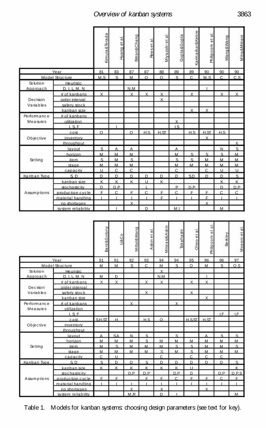
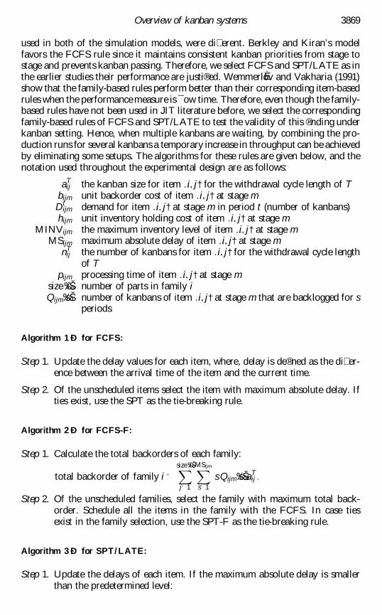
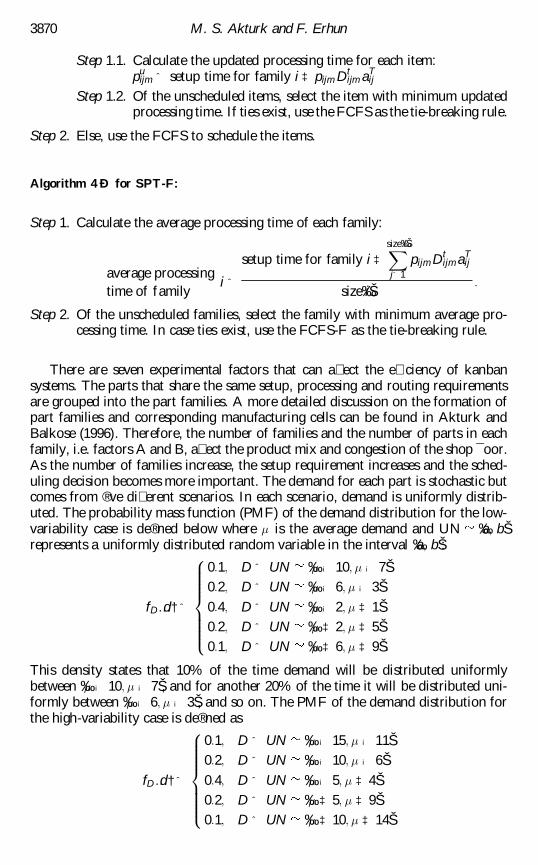
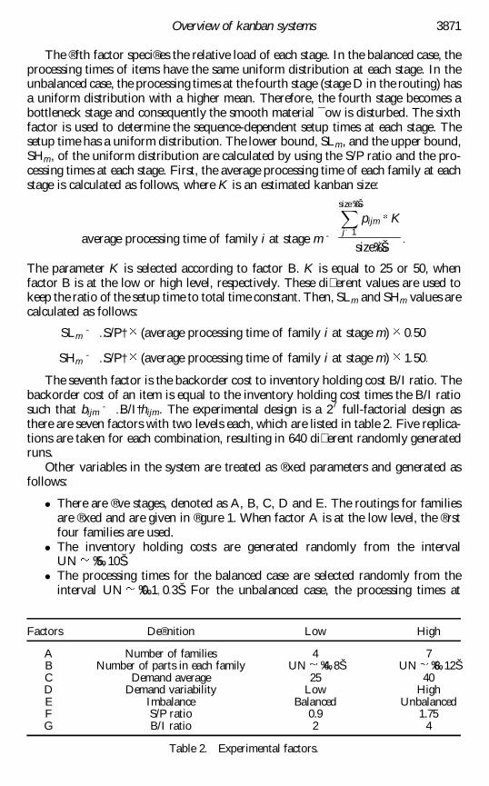
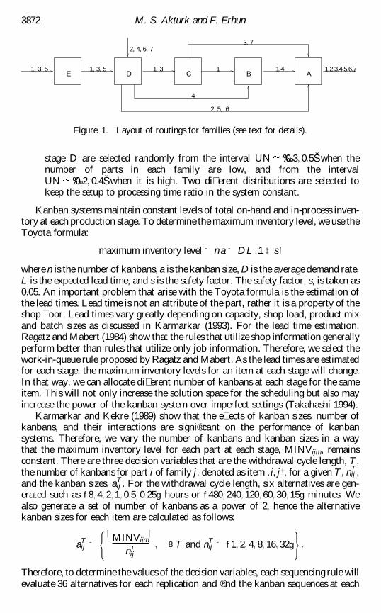
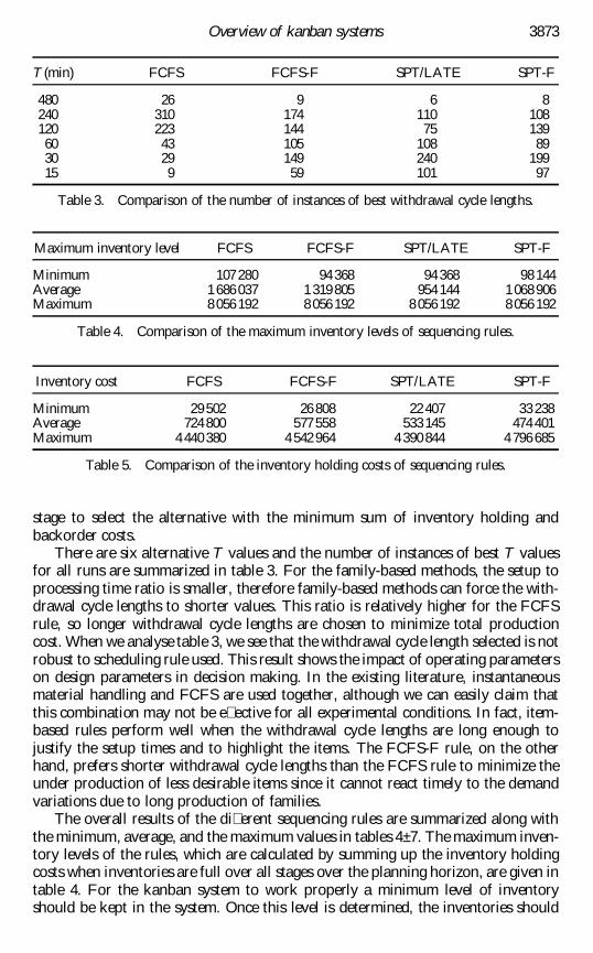
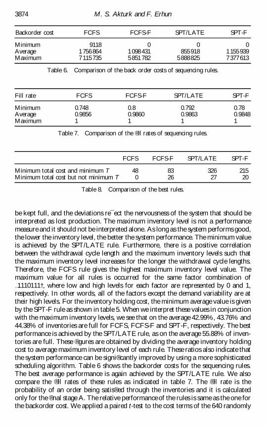
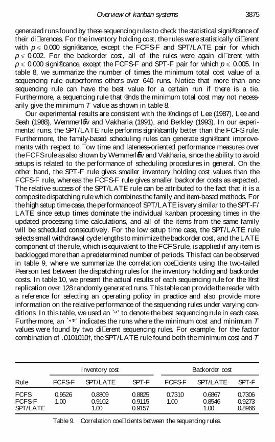
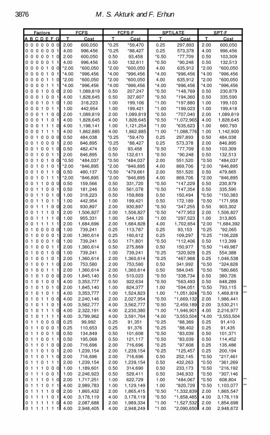
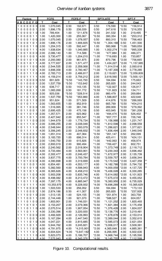
![cdn.buddy4study.comcdn.buddy4study.com/notes/12-pcm-nstse-2010-paper_0.pdfCLASS : If f(x) = , then f(x + y) . MATHEMATICS f(x — Y) [f (2x) + f (2y)] [f (x) — f (2y)] is : 2. 4](https://img.pdfslide.us/doc/110x75/5f0e4b497e708231d43e8aa3/cdn-class-if-fx-then-fx-y-mathematics-fx-a-y-f-2x-f-2y.jpg)


![funcy Documentation · string re_finder(f) re_tester(f) int or slice itemgetter(f) itemgetter(f) mapping lambda x: f[x] lambda x: f[x] set lambda x: x in f lambda x: x in f 2.1Supporting](https://img.pdfslide.us/doc/110x75/60bd10c8b4a628224a4ae997/funcy-documentation-string-refinderf-retesterf-int-or-slice-itemgetterf.jpg)


![K µ } } } ( ( d o W o v...ã Z \ ` a ^ : ^ F ] ä X X F [ X ä X X Z \ ^ ] Z : Y F [ ä X X F [ ä X X ã [ Z 9 ] : Z a ó Z \](https://img.pdfslide.us/doc/110x75/5f04ab847e708231d40f1ef5/k-d-o-w-o-v-z-a-f-x-x-f-x-x-x-z-z.jpg)


![7 o f , ] Ì X < µ X< } X < µ µ u f f < } µ f v f z º l º](https://img.pdfslide.us/doc/110x75/624eb863cc46354fb3067cdb/7-o-f-x-lt-xlt-x-lt-u-f.jpg)