Embed Size (px)
Citation preview
An Optimization Framework for Fixed-pointDigital Signal Processing
Lam Yuet Ming
A Thesis Submitted in Partial Fulfillment
of the Requirements for the Degree of
Master of Philosophy
in
Computer Science and Engineering
c©The Chinese University of Hong Kong
August, 2003
The Chinese University of Hong Kong holds the copyright of this thesis. Any
person(s) intending to use a part or the whole of the materials in this thesis in a
proposed publication must seek copyright release from the Dean of the Graduate
School.
An Optimization Framework for Fixed-point
Digital Signal Processing
Submitted by
Lam Yuet Ming
for the degree of Master of Philosophy in
Computer Science and Engineering
at the Chinese University of Hong Kong
in July, 2003
Abstract
Fixed-point hardware implementation of signal processing algorithms can often
achieve higher performance with lower computational requirements than a floating-
point implementation. However, the design of such systems is hard due to the
difficulties of addressing quantization issues. This work presents an optimization
approach to determining the wordlengths of signals in a fixed-point digital signal
processing system which enables users to achieve a given quality criteria with min-
imum hardware resources, resulting in reduced cost and perhaps lower power con-
sumption for VLSI implementation. These techniques lead to an automated op-
timization based design methodology for fixed-point based signal processing sys-
tems.
i
A framework involving a fixed-point class and an optimizer was developed.
The object oriented class, called Fixed, consists of a fixed-point class to analyze
fixed-point quantization effects. The Fixed class can simulate fixed-point opera-
tions such as addition, subtraction, multiplication and division where each operator
uses wordlengths of arbitrary precision. Calculations are done using both fixed-
point and floating-point formats and the floating-point calculations are used as a
reference to determine the quantization error. An optimizer based on the simplex
method and one-dimensional optimization approach was developed to minimize a
user defined cost function, thus finding an implementation which balances hardware
cost and user defined quality criteria.
This framework was applied to an isolated word recognition system based on
a vector quantizer (VQ) and a hidden Markov model (HMM) decoder using linear
predictive cepstral coefficients (LPCCs) as features. Utterances from the TIMIT
TI 46-word database were used for both training and recognition. The isolated
word recognition system was simulated using the fixed-point class, optimization
of wordlengths was done using the optimizer. A 28.5% hardware cost reduction
was achieved. Such an approach leads to clear advantages in both design effort
and hardware resource utilization over the traditional approaches where the same
wordlength is used for all operators.
ii
Acknowledgments
Special thanks will be given to Prof. LEONG Heng-Wai Philip for his help and
guidances through my master studies. I would also want to thank Prof. LEE, Kin
Hong and Prof. CHAN, Lai Wan for their suggestions and to be my thesis markers.
iii
Contents
1 Introduction 1
1.1 Motivation . . . . . . . . . . . . . . . . . . . . . . . . . . . . . . . 1
1.1.1 Difficulties of fixed-point design . . . . . . . . . . . . . . . 1
1.1.2 Why still fixed-point? . . . . . . . . . . . . . . . . . . . . 2
1.1.3 Difficulties of converting floating-point to fixed-point . . . . 2
1.1.4 Why wordlength optimization? . . . . . . . . . . . . . . . . 3
1.2 Objectives . . . . . . . . . . . . . . . . . . . . . . . . . . . . . . . 3
1.3 Contributions . . . . . . . . . . . . . . . . . . . . . . . . . . . . . 3
1.4 Thesis Organization . . . . . . . . . . . . . . . . . . . . . . . . . . 4
2 Review 5
2.1 Introduction . . . . . . . . . . . . . . . . . . . . . . . . . . . . . . 5
2.2 Simulation approach to address quantization issue . . . . . . . . . . 6
2.3 Analytical approach to address quantization issue . . . . . . . . . . 8
2.4 Implementation of speech systems . . . . . . . . . . . . . . . . . . 9
2.5 Discussion . . . . . . . . . . . . . . . . . . . . . . . . . . . . . . . 10
2.6 Summary . . . . . . . . . . . . . . . . . . . . . . . . . . . . . . . 11
3 Fixed-point arithmetic background 12
3.1 Introduction . . . . . . . . . . . . . . . . . . . . . . . . . . . . . . 12
3.2 Fixed-point representation . . . . . . . . . . . . . . . . . . . . . . 12
3.3 Fixed-point addition/subtraction . . . . . . . . . . . . . . . . . . . 14
iv
3.4 Fixed-point multiplication . . . . . . . . . . . . . . . . . . . . . . 16
3.5 Fixed-point division . . . . . . . . . . . . . . . . . . . . . . . . . . 18
3.6 Summary . . . . . . . . . . . . . . . . . . . . . . . . . . . . . . . 20
4 Fixed-point class implementation 21
4.1 Introduction . . . . . . . . . . . . . . . . . . . . . . . . . . . . . . 21
4.2 Fixed-point simulation using overloading . . . . . . . . . . . . . . 21
4.3 Fixed-point class implementation . . . . . . . . . . . . . . . . . . . 24
4.3.1 Fixed-point object declaration . . . . . . . . . . . . . . . . 24
4.3.2 Overload the operators . . . . . . . . . . . . . . . . . . . . 25
4.3.3 Arithmetic operations . . . . . . . . . . . . . . . . . . . . . 26
4.3.4 Automatic monitoring of dynamic range . . . . . . . . . . . 27
4.3.5 Automatic calculation of quantization error . . . . . . . . . 27
4.3.6 Array supporting . . . . . . . . . . . . . . . . . . . . . . . 28
4.3.7 Cosine calculation . . . . . . . . . . . . . . . . . . . . . . 28
4.4 Summary . . . . . . . . . . . . . . . . . . . . . . . . . . . . . . . 29
5 Speech recognition background 30
5.1 Introduction . . . . . . . . . . . . . . . . . . . . . . . . . . . . . . 30
5.2 Isolated word recognition system overview . . . . . . . . . . . . . 30
5.3 Linear predictive coding processor . . . . . . . . . . . . . . . . . . 32
5.3.1 The LPC model . . . . . . . . . . . . . . . . . . . . . . . . 32
5.3.2 The LPC processor . . . . . . . . . . . . . . . . . . . . . . 33
5.4 Vector quantization . . . . . . . . . . . . . . . . . . . . . . . . . . 36
5.5 Hidden Markov model . . . . . . . . . . . . . . . . . . . . . . . . 38
5.6 Summary . . . . . . . . . . . . . . . . . . . . . . . . . . . . . . . 40
6 Optimization 41
6.1 Introduction . . . . . . . . . . . . . . . . . . . . . . . . . . . . . . 41
6.2 Simplex Method . . . . . . . . . . . . . . . . . . . . . . . . . . . . 41
v
6.2.1 Initialization . . . . . . . . . . . . . . . . . . . . . . . . . 42
6.2.2 Reflection . . . . . . . . . . . . . . . . . . . . . . . . . . . 42
6.2.3 Expansion . . . . . . . . . . . . . . . . . . . . . . . . . . . 44
6.2.4 Contraction . . . . . . . . . . . . . . . . . . . . . . . . . . 44
6.2.5 Stop . . . . . . . . . . . . . . . . . . . . . . . . . . . . . . 45
6.3 One-dimensional optimization approach . . . . . . . . . . . . . . . 45
6.3.1 One-dimensional optimization approach . . . . . . . . . . . 46
6.3.2 Search space reduction . . . . . . . . . . . . . . . . . . . . 47
6.3.3 Speeding up convergence . . . . . . . . . . . . . . . . . . . 48
6.4 Summary . . . . . . . . . . . . . . . . . . . . . . . . . . . . . . . 50
7 Word Recognition System Design Methodology 51
7.1 Introduction . . . . . . . . . . . . . . . . . . . . . . . . . . . . . . 51
7.2 Framework design . . . . . . . . . . . . . . . . . . . . . . . . . . . 51
7.2.1 Fixed-point class . . . . . . . . . . . . . . . . . . . . . . . 52
7.2.2 Fixed-point application . . . . . . . . . . . . . . . . . . . . 53
7.2.3 Optimizer . . . . . . . . . . . . . . . . . . . . . . . . . . . 53
7.3 Speech system implementation . . . . . . . . . . . . . . . . . . . . 54
7.3.1 Model training . . . . . . . . . . . . . . . . . . . . . . . . 54
7.3.2 Simulate the isolated word recognition system . . . . . . . 56
7.3.3 Hardware cost model . . . . . . . . . . . . . . . . . . . . . 57
7.3.4 Cost function . . . . . . . . . . . . . . . . . . . . . . . . . 58
7.3.5 Fraction size optimization . . . . . . . . . . . . . . . . . . 59
7.3.6 One-dimensional optimization . . . . . . . . . . . . . . . . 61
7.4 Summary . . . . . . . . . . . . . . . . . . . . . . . . . . . . . . . 63
8 Results 64
8.1 Model training . . . . . . . . . . . . . . . . . . . . . . . . . . . . 64
8.2 Simplex method optimization . . . . . . . . . . . . . . . . . . . . . 65
8.2.1 Simulation platform . . . . . . . . . . . . . . . . . . . . . 65
vi
8.2.2 System level optimization . . . . . . . . . . . . . . . . . . 66
8.2.3 LPC processor optimization . . . . . . . . . . . . . . . . . 67
8.2.4 One-dimensional optimization . . . . . . . . . . . . . . . . 68
8.3 Speeding up the optimization convergence . . . . . . . . . . . . . . 71
8.4 Optimization criteria . . . . . . . . . . . . . . . . . . . . . . . . . 73
8.5 Summary . . . . . . . . . . . . . . . . . . . . . . . . . . . . . . . 75
9 Conclusion 76
9.1 Search space reduction . . . . . . . . . . . . . . . . . . . . . . . . 76
9.2 Speeding up the searching . . . . . . . . . . . . . . . . . . . . . . 77
9.3 Optimization criteria . . . . . . . . . . . . . . . . . . . . . . . . . 77
9.4 Flexibility of the framework design . . . . . . . . . . . . . . . . . . 78
9.5 Further development . . . . . . . . . . . . . . . . . . . . . . . . . 78
Bibliography 80
vii
List of Figures
3.1 Two’s complement integer format . . . . . . . . . . . . . . . . . . 13
3.2 Fixed-point representation for fraction number . . . . . . . . . . . . 13
3.3 Parallel adder . . . . . . . . . . . . . . . . . . . . . . . . . . . . . 15
3.4 Two’s complement multiplication . . . . . . . . . . . . . . . . . . 17
3.5 Block diagram of divider using restoring-division . . . . . . . . . . 20
4.1 Fixed-point class declaration . . . . . . . . . . . . . . . . . . . . . 23
4.2 IEEE 754 double-precision format . . . . . . . . . . . . . . . . . . 25
4.3 Arithmetic calculation using fixed-point object . . . . . . . . . . . 26
5.1 Isolated word recognition system . . . . . . . . . . . . . . . . . . . 31
5.2 LPC model of speech . . . . . . . . . . . . . . . . . . . . . . . . . 33
5.3 Block diagram of the LPC feature analysis . . . . . . . . . . . . . . 34
5.4 Frame blocking process . . . . . . . . . . . . . . . . . . . . . . . . 35
5.5 Vector quantization process . . . . . . . . . . . . . . . . . . . . . . 36
5.6 Left-to-Right HMM . . . . . . . . . . . . . . . . . . . . . . . . . . 38
5.7 Trellis representation of Left-to-Right HMM . . . . . . . . . . . . . 39
6.1 Reflection . . . . . . . . . . . . . . . . . . . . . . . . . . . . . . . 43
6.2 One-dimensional optimization . . . . . . . . . . . . . . . . . . . . 47
6.3 Golden section search . . . . . . . . . . . . . . . . . . . . . . . . . 49
7.1 Block diagram of the framework . . . . . . . . . . . . . . . . . . . 52
7.2 Optimizer executes fixed-point application iteratively . . . . . . . . 54
viii
7.3 Overview of isolated word recognition system optimization flow . . 55
7.4 System level optimization using simplex method . . . . . . . . . . 60
7.5 LPC processor’s fraction size optimization using simplex method . . 61
7.6 System level optimization using one-dimensional optimization . . . 62
8.1 Recognition accuracy for different configurations of VQ codebook
size and number of HMM states . . . . . . . . . . . . . . . . . . . 65
8.2 Recognition accuracy when sweep the fraction size of the whole
system . . . . . . . . . . . . . . . . . . . . . . . . . . . . . . . . . 68
8.3 Recognition accuracy when sweep the fraction size of the LPC pro-
cessor . . . . . . . . . . . . . . . . . . . . . . . . . . . . . . . . . 69
8.4 Recognition accuracy when sweep the fraction size of the VQ . . . 70
8.5 Recognition accuracy when sweep the fraction size of the HMM
decoder . . . . . . . . . . . . . . . . . . . . . . . . . . . . . . . . 71
ix
List of Tables
3.1 Fixed-point representation of fractional number 2.875 using differ-
ent notation . . . . . . . . . . . . . . . . . . . . . . . . . . . . . . 14
8.1 System level optimization using the simplex method . . . . . . . . . 66
8.2 LPC processor optimization using the simplex method . . . . . . . 67
8.3 System level optimization using one-dimensional optimization . . . 72
8.4 Result comparison between applying exhaustive search, the golden
section search and simplex method in system level optimization . . 73
8.5 Results using different optimization criteria in LPC processor opti-
mization . . . . . . . . . . . . . . . . . . . . . . . . . . . . . . . . 74
x
Chapter 1
Introduction
1.1 Motivation
1.1.1 Difficulties of fixed-point design
The productivity of digital integrated circuit designers has been significantly im-
proved by using high level synthesis techniques in recent times, these techniques
can allow the designers concentrate more on high level issues, e.g. algorithm and
architecture. Although higher productivity is obtained, the difficulties of addressing
quantization effects in designing fixed-point system remain unchanged.
Because of the limited dynamic range of fixed-point representations of signals
in a design, underflow and overflow problems may occur. When designing a fixed-
point system, the designer needs to assign appropriate wordlength to each variable.
Simulation programs, typically constructed using high level languages are of-
ten used to develop and verify the algorithms. Unfortunately, up to now, there is
no direct support for the representation of fixed-point arbitrary precision fractional
numbers in high level programming languages and digital signal processing (DSP)
chips. Fixed-point system design typically starts from a floating-point description
which offers wider dynamic range and is hence less susceptible to quantization er-
rors.
1
Chapter 1 Introduction 2
1.1.2 Why still fixed-point?
For signals with low dynamic range, fixed-point arithmetic offers advantages over
floating-point in terms of performance, power consumption and hardware cost since
fixed-point arithmetic is more efficient, a floating-point implementation may double
or triple the hardware requirements compared with corresponding fixed-point im-
plementation [Kai79]. Although there are some DSP chips support floating-point
arithmetic, experimental results shows that using fixed-point arithmetic can reach
higher clock rate [BM91], and lower cost, e.g. lower memory usage [FBM98]. Be-
cause of these benefits, fixed-point arithmetic is often used in a wide range of DSP
applications where signals have relatively low dynamic ranges.
1.1.3 Difficulties of converting floating-point to fixed-point
Since fixed-point arithmetic is widely used in hardware implementations, the prob-
lem of converting an algorithmic description, which typically uses floating-point
arithmetic in some high level programming language such as C, to a hardware effi-
cient fixed-point description needs to be addressed. This process is tedious and error
prone, because of the limited dynamic range of fixed-point representations. Some
issues, e.g. overflow, underflow, rounding/truncation error, should be handled dur-
ing transformation. Typical design analyzes the quantization effect manually by
observing the ranges of variables and assign enough wordlength for each variable,
but this is low efficiency and time consuming. As a result, bit-accurate simulation
of the fixed-point design is necessary to analyze these quantization effects on an
algorithmic level in order to be realized on hardware, in this way, the designer can
concentrate on higher level design issues.
Chapter 1 Introduction 3
1.1.4 Why wordlength optimization?
Longer wordlengths will result in smaller quantization errors, but in order to reach a
given error level, some intermediate variables, which will not contribute to the quan-
tization error of final result, can be truncated in wordlengths. Wordlength optimiza-
tion can be done based on this phenomenon. There are a number of advantages for
wordlength optimization, such as lower cost and lower power consumption. These
advantages can benefit some low power and small area designs, e.g. mobile devices,
smart cards, PDAs, etc.
1.2 Objectives
The main objective of this research work was to develop a methodology for the
design and optimization of fixed-point system. The detailed research aims were:
• Formulate a systematic methodology for addressing quantization issues in the
fixed-point system.
• Explore the utility of this approach using isolated word recognition system as
a realistic example.
1.3 Contributions
In this work, a framework was introduced to address the quantization issue in fixed-
point systems. The main contributions of this dissertation are as follows:
• A C++ fixed-point class, called Fixed, was developed to simulate fixed-point
arithmetic. All variables in an original floating-point description are changed
to be of the Fixed type. Using overloading, the fixed-point description can be
made to be very similar to the floating-point description, so minimal changes
to the source code are required.
Chapter 1 Introduction 4
• An optimizer was developed to perform hardware cost/wordlength optimiza-
tion, the optimizer can be used to minimize a cost function which is designed
by the user. Since wordlength is monotonic decreasing with quantization er-
ror and monotonic increasing with hardware cost, if the cost function takes
the error and hardware cost into account, optimal wordlengths can be found
for all variables which can balance the hardware cost and error.
• This framework was applied to an isolated word recognition system, the sys-
tem was simulated using the fixed-point class, optimization of wordlength
was done using the optimizer. The design is very flexible, each part is de-
veloped independently, different experiments can be done easily. Optimal
wordlengths were found which can balance the hardware cost and recogni-
tion accuracy.
• To the best of my knowledge, this is the first time an optimization of variable
wordlengths has been applied to the isolated word recognition problem. This
study has led to insights into the precision requirements in such systems.
1.4 Thesis Organization
In Chapter 2, a review of related work on fixed-point quantization issues and speech
system implementation is given. Chapter 3 introduces background to fixed-point
arithmetic and Chapter 4 presents the implementation of the fixed-point class. Chap-
ter 5 introduces the background to an isolated word recognition system and Chapter
6 introduces the optimization background. In Chapter 7, the framework and word
recognition system design methodology are presented. Some experimental results
are given in Chapter 8. Finally, the conclusion is presented in Chapter 9.
Chapter 2
Review
2.1 Introduction
Fixed-point hardware implementations of signal processing algorithms can often
achieve higher performance with lower computational requirements than corre-
sponding floating-point implementations. However, the design of such systems is
hindered by the difficulty of addressing quantization issues, which includes quanti-
zation effect analysis of fixed-point system and hardware cost/wordlength optimiza-
tion.
Design of such systems center around analyzing and improving the quantization
error of the fixed-point system, finding the wordlength requirements for fixed-point
variables, and optimizing wordlengths for fixed-point variables which can reach
specified quality criteria or balance the performance and hardware cost. In this
chapter, some related work are reviewed. Since this work used an isolated word
recognition system as an example, the implementations of speech systems are also
reviewed.
This chapter is organized as follows. Section 2.2 presents the work using sim-
ulation approaches to address the quantization issue while Section 2.3 presents the
work using analytical approaches. Section 2.4 introduces some implementations of
speech systems. Section 2.5 and 2.6 are discussion and summary.
5
Chapter 2 Review 6
2.2 Simulation approach to address quantization is-
sue
The simulation approach collects quantization information, e.g. quantization er-
ror, through simulation using realistic data. Wordlengths of variables are chosen
heuristically while observing some quality criterion, this process is repeated with
different configurations of wordlengths and stop when a specified quality criterion
is met. One drawback using this approach is the long simulation time, especially
for some complex systems. The other drawback is, the results obtained through
simulation is dataset dependent and it is hard to choose a representative dataset.
Since manual fixed-point design is error prone, simulation of fixed-point design
or transformation from floating-point descriptions to fixed-point implementations is
required. The integer type in a high level programming language can be used to
simulate a fixed-point format [RJ87]. C++ object classes have also been used to
simulate a fixed-point format [WM94], a fixed-point format fraction number being
represented using an object class, some information, e.g. the amplitude, wordlength,
are stored in the object class and the calculation is handled by the class. The object
class proposed by Jersak and Willems [MM98] used a similar approach.
Kim et. al. [SKW95] proposed C++ object classes to simulate fixed-arithmetic
using operator overloading. Firstly, the floating-point type in the original code is re-
placed with a range estimating C++ class “fSig”, then a simulation-based approach
is applied to determine the range of variables using realistic data. Another C++
object class, called “gFix”, is used to simulate fixed-point arithmetic and record
the error. The wordlengths of variables were determined based on these collected
information. Based on this work, Sung and Kum [WK95] proposed a searching-
based approach to perform wordlength optimization. The fixed-point system is
simulated using C++ object class, optimization is done to find minimum hardware
cost implementation while meeting a specific error requirement. Wordlength opti-
mization was done using two approaches, the heuristic and exhaustive approaches.
Chapter 2 Review 7
Firstly, the lower bound of wordlength of each variables are determined by set-
ting the wordlength of other variables to very large. For the heuristic approach,
each variable starts from the lower bound, and the wordlength of each variable is
increased alternately until the error requirement is satisfied. For the exhaustive ap-
proach, wordlengths of all variables are increased simultaneously, until the error
requirements are satisfied. The wordlength of each variable are then decreased until
the error requirement test fails. A tool to transform a floating-point program into
fixed-point implementation using ANSI-C integer types proposed by Kum et. al.
[KJW00] was also based on the developed object class [SKW95]. Wordlengths of
variables are determined based on the collected quantization information after sim-
ulation. Moreover, the number of shift operations in the transformed code is mini-
mized, the minimization is done by minimize a cost function which take account of
the number of shift operations. The number of shift operations is hardware depen-
dent, for a DSP processor with a barrel shifter, like TMS320C25, TMS320C50 and
TMS320C60, the cost of a shift operation is one cycle, for DSP processor without a
barrel shift, like Motorola 56000, the cost of a n-bits shift operation is n cycles. Fi-
nally, the floating-point type is replaced by an integer type, and appropriate scaling
codes are inserted.
Keding et. al. [HMMH98] proposed a system called FRIDGE to find the wordlength
requirements of variables, an interpolative approach is introduced, and this approach
depends much on human knowledge. Fixed-point variables are modeled as a C++
class. The designer should input some information to some fixed-point variables
which are critical or already known in the system, such as wordlength, integer
wordlength. Wordlengths of other variables are determined using propagation rules
and the analysis of the data flow. Simulation is then applied to check if the accuracy
constraints are fulfilled. If the requirement is not achieved, the designer needs to
make adjustment to the inputted information. Another drawback of this work is the
designer need to put much efforts during optimization.
Chapter 2 Review 8
The work proposed by Chang and Hauck [MS02] address on wordlength opti-
mization in the MATLAB environment. A piece of code is appended into to original
code to find the dynamic range of each variable, the dynamic range can be used to
calculate the wordlengths of variables, these wordlengths are considered as lower
bound. Propagation rules are used to find an upper bound for the wordlength of
each variable. During optimization, for each variable, the wordlength is set to the
lower bound, then the impact of that change over all variables is propagated and the
change in hardware cost for that variable is recorded. This procedure is repeated
for other variables and the change in hardware cost is sorted in decreasing order.
This information is presented to the designer to decide which variables should be
more tightly constrained in wordlength. One drawback with this approach is, the
selection process is very much dependent on human experience.
2.3 Analytical approach to address quantization is-
sue
Analytical approaches analyze the quantization error of computation based on a
theoretical framework, an error expression often being derived [P. 91, SW98]. The
wordlength of a fixed-point variable are usually derived from the signal-flow graph,
local annotations, interpolation, and propagation of ranges of variables. This ap-
proach can give true upper bounds and achieve a faster run time than a simulation
approach, but the result may be very conservative and lead to a gross overestimation
of variable wordlengths [RLP+99].
Fiore [Pau98] addressed the quantization error of the addition of two uncorre-
lated values that are truncated/rounded prior to addition. Two methods were in-
troduced for rounding which can reduce the hardware complexity and maintain a
certain variance. The first method called LR, it basically ORing the most significant
Chapter 2 Review 9
bits of the parts to be truncated and input the result as carry input of the least sig-
nificant bit of the adder chain. The second method called RLR, simply inputs 1 as
carry input to the least significant bit of the adder chain. Some experiments shows
that the variance using LR/RLR is close to the results using truncation/rounding.
Wadekar and Parker [SA98] proposed to reduce the wordlength of some vari-
ables that do not contribute significantly to the final result. A worse-case error
estimation model is introduced, the error propagated from the input to output. Two
examples, discrete cosine transform and 5× 5 matrix determinant, were used and a
genetic algorithm was applied to minimize the hardware cost and reach a specified
error bound at the same time. In the genetic algorithm, the quality of the final result
depends on the population size [Voj02], but the population size is bounded by the
available computing resources, since the computational power is proportional to the
population size.
The work proposed by Cmar et. al. [RLP+99] using both analytical and simu-
lation approaches. The integer size of a fixed-point variable is determined by using
a statistical method or propagation of dynamic range. But, as pointed out by the
author, range propagation can become unstable and cause explosion when applied
to feedback signals. To determine the fraction size of fixed-point variable, a simula-
tion approach is used. An object class is introduced to represent a variable in fixed-
point format, simulation is carried out to collect the error between a fixed-point
and floating-point system, fraction size is determined by comparing the calculation
results between fixed-point and floating-point arithmetic.
2.4 Implementation of speech systems
Optimizing recognition accuracy and real time performance are the major consider-
ations of most previous approaches. Some popular DSP chips such as the TMS320
series [KGR97] have been widely used for implementing speech recognition sys-
tems [YY00, KJK95, NNS+99]. Kim et. al. [SIYS96] proposed a VLSI chip for
Chapter 2 Review 10
isolated speech recognition system which can recognize 1000 isolated words per
second. Bliss and Scharf [WL89] proposed a ring architecture to perform hidden
Markov model (HMM) decoding in parallel. In this architecture, each processing el-
ement will calculate predecessors serially. N processing elements can compute the
score for all HMM states in parallel. Under the development of field-programmable
gate array (FPGA) technique, FPGA chips have higher density and clock rate, im-
plement more complicated systems on FPGA chip becomes realizable, it is often
chosen to achieve high performance, Vargas et. al. [FRD01] proposed a FPGA
implementation of a HMM decoder which is 500 times faster than a classic imple-
mentation. A speech recognition system proposed by Melnikoff et. al. [SSM02],
can process speech 75 times real time using a Xilinx Virtex XCV1000 chip.
Hidden Markov models (HMMs) are widely used in modern speech recognition
systems because HMM-based speech recognition systems have proven to yield high
recognition accuracy. Some speech systems focus on improving implementation
of HMM to get better recognition accuracy. Zhang et. al. [YCR+94] proposed
using multiple hidden Markov models, each word in the vocabulary contains three
vector quantization methods and three hidden Markov models. Gholampour and
Nayebi [IK99] introduced a cascade HMM/ANN model to improve the recognition
accuracy.
2.5 Discussion
Analytical approaches require extensive knowledge of both the algorithm and hard-
ware architecture, moreover, it is hard to develop an error model for complicated
systems. Wordlength optimization is tedious, in the work proposed by Hui et. al.
[GKZ98], in order to find an optimal allocation of a variable precision, the authors
needed to implement several systems using different numerical formats, such as
single fixed-point format, double fixed-point format and floating-point format. A
Chapter 2 Review 11
simulation-based approach seems be a better choice, since it can reduce the bur-
den of designer, all jobs being done by computer. But some simulation approaches,
e.g. [MS02], still require the designer to be involved in the optimization process,
the designer should analyze the simulation result and make decision to constrain
which variables. Although some work has been done to optimize some fixed-point
systems using a searching-based method, e.g. [WK95], the goal of this work is to
provide a tool for assisting fixed-point system design and optimization, using this
tool, designers can have a much clearer idea of the wordlength requirements of their
hardware design.
Previous fixed-point implementations of speech recognition systems concen-
trated on optimizing recognition accuracy and real time performance, and quanti-
zation effects in fixed-point arithmetic were seldom directly addressed. With im-
provements in speech models and VLSI technology, speech recognition accuracy
is much higher than in the past, and designing a speech recognition system with
real time performance is not that difficult. However quantization issues remain
a problem when designing a fixed-point hardware system, this work performing
wordlength/hardware cost optimization of an isolated word recognition system, it is
more complicated than most of previous optimization work for filters.
2.6 Summary
In this chapter, we have review some related work on fixed-point design and imple-
mentation, including the simulation of fixed-point arithmetic, analytical and simu-
lation approach to address the quantization effect and optimization. Some imple-
mentations of speech system also reviewed.
Chapter 3
Fixed-point arithmetic background
3.1 Introduction
Fixed-point arithmetic is widely used in digital signal processing systems, because
it has a simpler implementation than floating-point arithmetic. A brief introduction
to fixed-point arithmetic is given in this chapter.
This chapter is organized as follows. Section 3.2 introduces fixed-point num-
ber representations. In Section 3.3, fixed-point addition/subtraction is introduced.
Fixed-point multiplication is introduced in Section 3.4 and fixed-point division is
described in 3.5, the last section is the summary.
3.2 Fixed-point representation
There are several notations commonly used to represent a binary integer, such as
sign-and-magnitude, one’s complement and two’s complement notations. Two’s
complement format is the most commonly used format [Amo94].
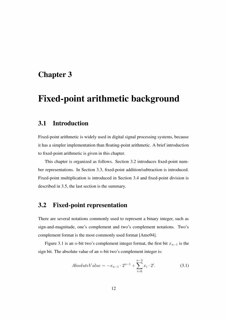
Figure 3.1 is an n-bit two’s complement integer format, the first bit xn−1 is the
sign bit. The absolute value of an n-bit two’s complement integer is:
AbsoluteV alue = −xn−1 · 2n−1 +n−2∑
i=0
xi · 2i. (3.1)
12
Chapter 3 Fixed-point arithmetic background 13
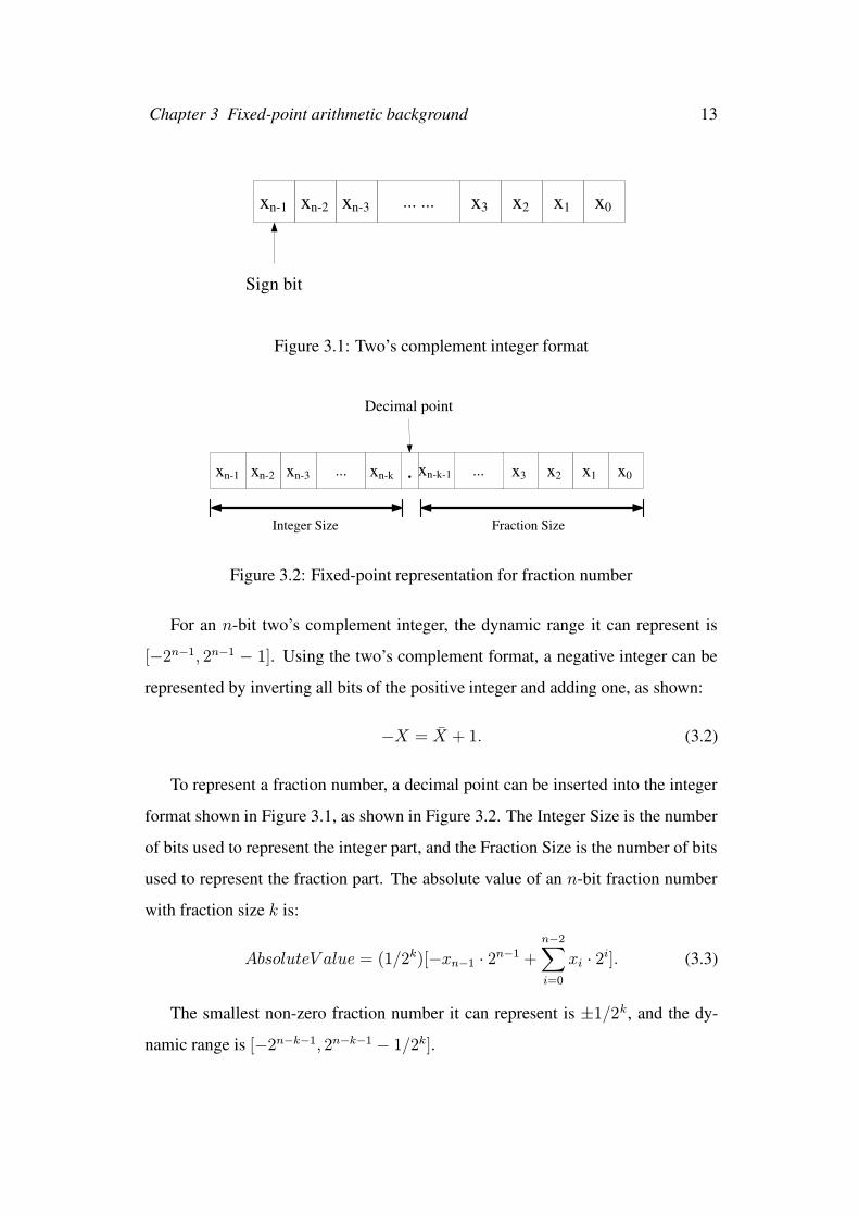
Sign bit
... ... x 0 x n - 1 x n - 2 x n - 3 x 1 x 2 x 3
Figure 3.1: Two’s complement integer format
Integer Size Fraction Size
... x 0 x n - 1 x n - 2 x n - 3 x 1 x 2 x 3 x n - k . ... x n - k - 1
Decimal point
Figure 3.2: Fixed-point representation for fraction number
For an n-bit two’s complement integer, the dynamic range it can represent is
[−2n−1, 2n−1 − 1]. Using the two’s complement format, a negative integer can be
represented by inverting all bits of the positive integer and adding one, as shown:
−X = X + 1. (3.2)
To represent a fraction number, a decimal point can be inserted into the integer
format shown in Figure 3.1, as shown in Figure 3.2. The Integer Size is the number
of bits used to represent the integer part, and the Fraction Size is the number of bits
used to represent the fraction part. The absolute value of an n-bit fraction number
with fraction size k is:
AbsoluteV alue = (1/2k)[−xn−1 · 2n−1 +n−2∑
i=0
xi · 2i]. (3.3)
The smallest non-zero fraction number it can represent is ±1/2k, and the dy-
namic range is [−2n−k−1, 2n−k−1 − 1/2k].
Chapter 3 Fixed-point arithmetic background 14
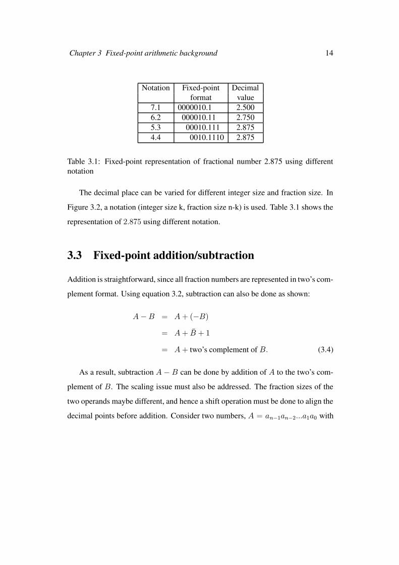
Notation Fixed-point Decimalformat value
7.1 0000010.1 2.5006.2 000010.11 2.7505.3 00010.111 2.8754.4 0010.1110 2.875
Table 3.1: Fixed-point representation of fractional number 2.875 using differentnotation
The decimal place can be varied for different integer size and fraction size. In
Figure 3.2, a notation (integer size k, fraction size n-k) is used. Table 3.1 shows the
representation of 2.875 using different notation.
3.3 Fixed-point addition/subtraction
Addition is straightforward, since all fraction numbers are represented in two’s com-
plement format. Using equation 3.2, subtraction can also be done as shown:
A−B = A + (−B)
= A + B + 1
= A + two’s complement of B. (3.4)
As a result, subtraction A − B can be done by addition of A to the two’s com-
plement of B. The scaling issue must also be addressed. The fraction sizes of the
two operands maybe different, and hence a shift operation must be done to align the
decimal points before addition. Consider two numbers, A = an−1an−2...a1a0 with
Chapter 3 Fixed-point arithmetic background 15
+
a3 b3
s3
+
a2 b2
s2
+
a1 b1
s1
+
a0 b0
s0
Carry in Carry out
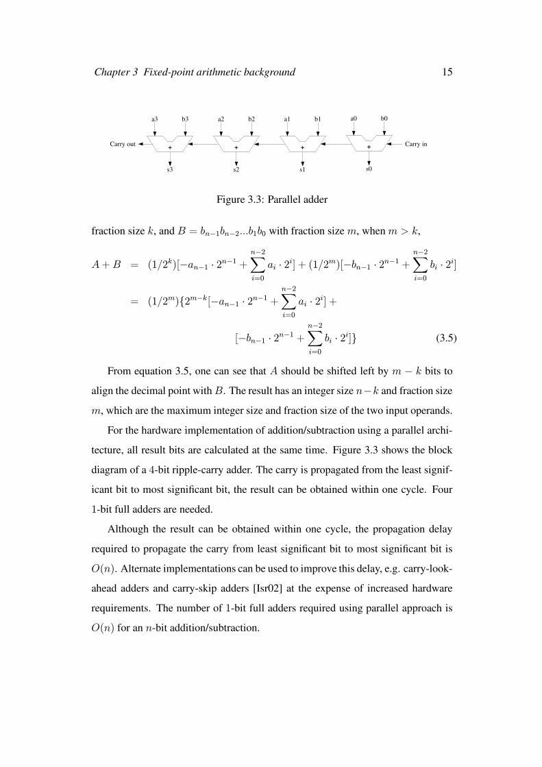
Figure 3.3: Parallel adder
fraction size k, and B = bn−1bn−2...b1b0 with fraction size m, when m > k,
A+B = (1/2k)[−an−1 · 2n−1 +n−2∑
i=0
ai · 2i] + (1/2m)[−bn−1 · 2n−1 +n−2∑
i=0
bi · 2i]
= (1/2m){2m−k[−an−1 · 2n−1 +n−2∑
i=0
ai · 2i] +
[−bn−1 · 2n−1 +n−2∑
i=0
bi · 2i]} (3.5)
From equation 3.5, one can see that A should be shifted left by m − k bits to
align the decimal point withB. The result has an integer size n−k and fraction size
m, which are the maximum integer size and fraction size of the two input operands.
For the hardware implementation of addition/subtraction using a parallel archi-
tecture, all result bits are calculated at the same time. Figure 3.3 shows the block
diagram of a 4-bit ripple-carry adder. The carry is propagated from the least signif-
icant bit to most significant bit, the result can be obtained within one cycle. Four
1-bit full adders are needed.
Although the result can be obtained within one cycle, the propagation delay
required to propagate the carry from least significant bit to most significant bit is
O(n). Alternate implementations can be used to improve this delay, e.g. carry-look-
ahead adders and carry-skip adders [Isr02] at the expense of increased hardware
requirements. The number of 1-bit full adders required using parallel approach is
O(n) for an n-bit addition/subtraction.
Chapter 3 Fixed-point arithmetic background 16
3.4 Fixed-point multiplication
Let the multiplier and multiplicand beA = an−1an−2...a1a0 andB = bn−1bn−2...b1b0
respectively. A sequential multiplication operates by scanning the multiplier A bit
by bit, and forming the product ajB for the jth bit, a new partial product P (j+1) is
obtained by summing ajB and previous partial product P (j), a total of n − 1 itera-
tions is required to calculate the final product. The expression for this recursive step
is
P (j+1) = P (j) + aj ·B · 2j; (3.6)
where P (0) = 0. One can see that product ajB is aligned before added to
previous partial product P (j), it is because the weight of aj+1 is double that of aj.
As a result, at step j, ajB should shift to left j bits. Using this notation, P (n−1) can
be calculated as
P (n−1) = P (n−2) + an−2 ·B · 2n−2
= P (n−3) + an−3 ·B · 2n−3 + an−2 ·B · 2n−2
= ......
= a0 ·B · 20 + a1 ·B · 21 + ...+ an−3 ·B · 2n−3 + an−2 ·B · 2n−2
=n−2∑
j=0
aj ·B · 2j
= (n−2∑
j=0
aj · 2j) ·B (3.7)
Using the above result, if the multiplier A and multiplicandB are both positive,
the product can be calculated as
Product = A ·B = (n−1∑
j=0
aj · 2j) ·B
= (n−2∑
j=0
aj · 2j) ·B (since an−1 = 0)
= P (n−1) (3.8)
Chapter 3 Fixed-point arithmetic background 17
b2 b1 b0
a2 a1 a0 x
b0xa0 b1xa0 b2xa0
b0xa1 b1xa1 b2xa1
b0xa2 b1xa2 b2xa2
s2 s1 s0 s4 s3
b2xa0 sign
extended
q2 q1 q0 q3 q3
Carry 1
+
+
sign extended
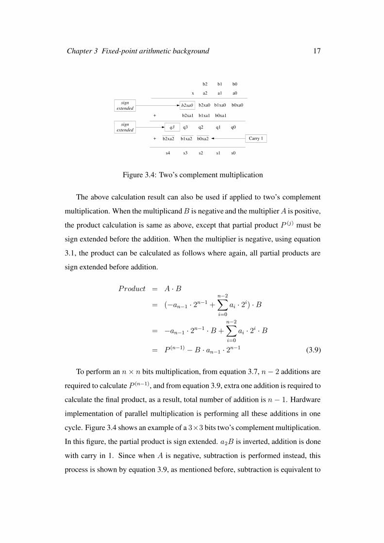
Figure 3.4: Two’s complement multiplication
The above calculation result can also be used if applied to two’s complement
multiplication. When the multiplicandB is negative and the multiplierA is positive,
the product calculation is same as above, except that partial product P (j) must be
sign extended before the addition. When the multiplier is negative, using equation
3.1, the product can be calculated as follows where again, all partial products are
sign extended before addition.
Product = A ·B
= (−an−1 · 2n−1 +n−2∑
i=0
ai · 2i) ·B
= −an−1 · 2n−1 ·B +n−2∑
i=0
ai · 2i ·B
= P (n−1) −B · an−1 · 2n−1 (3.9)
To perform an n× n bits multiplication, from equation 3.7, n− 2 additions are
required to calculate P (n−1), and from equation 3.9, extra one addition is required to
calculate the final product, as a result, total number of addition is n− 1. Hardware
implementation of parallel multiplication is performing all these additions in one
cycle. Figure 3.4 shows an example of a 3×3 bits two’s complement multiplication.
In this figure, the partial product is sign extended. a2B is inverted, addition is done
with carry in 1. Since when A is negative, subtraction is performed instead, this
process is shown by equation 3.9, as mentioned before, subtraction is equivalent to
Chapter 3 Fixed-point arithmetic background 18
addition of one operand to the two’s complement of the other operand as shown by
equation 3.4.
Since summing P (j) and ajB is an n-bit addition, and total number of iteration
is n− 1, in order to perform summation of all partial products in one cycle, by ap-
proximation,O(n2) 1-bit full adders should be used for an n×n bits multiplication.
Some parallel architectures, such as array structure [Isr02], can be used to perform
this parallel addition.
3.5 Fixed-point division
Consider a division A/B, assume the quotient is Q and the remainder is R which
are defined by
A = B ·Q+R. (3.10)
Assuming that all variables are unsigned firstly, a sequence of subtractions and
shifts is done to determine the quotient Q = q0q1...qn−1. At iteration i, the remain-
der is compared to the divisorB, if the remainder is larger thanB, the corresponding
quotient bit is set to 1, otherwise, set to 0. The expression for this recursive step is
ri = ri−1 − qi−1 ·B · 2n−i, (3.11)
where ri is the remainder at iteration i and r0 = A. qi−1 is determined by
comparing ri−1 to B · 2n−i. The final remainder can be obtained after n iterations
as
rn = rn−1 − qn−1 ·B · 20
= rn−2 − qn−2 ·B · 21 − qn−1 ·B · 20
= ......
= r0 − q0 ·B · 2n − q1 ·B · 2n−1 − ...− qn−2 ·B · 21 − qn−1 ·B · 20
= r0 − (q0 · 2n + q1 · 2n−1 + ...+ qn−2 · 21 + qn−1 · 20) ·B
= A−Q ·B, (3.12)
Chapter 3 Fixed-point arithmetic background 19
where rn = R. For two’s complement division, the process is similar, except
that to determine the quotient bit, either subtraction or addition is used based on the
signs of ri−1 and B, as shown below:
if ri−1 and B have the same sign, then {ri = ri−1 − qi−1 ·B · 2n−i;}else {ri = ri−1 + qi−1 ·B · 2n−i;}
if ri and ri−1 have the same sign, then {set qi−1 to 1;
}else {set qi−1 to 0;
ri = ri−1;
}
From the above algorithm, one can see that, when ri and ri−1 have different
signs, ri is restored to the previous value ri−1. This method is therefore called
restoring division [CZS02]. In this method, the main arithmetic operations are ad-
dition and subtraction ri = ri−1± qi−1 ·B ·2n−i. As mentioned by previous section,
subtraction can be done using addition, an n-bit adder is needed. AlthoughB is left
shifted n − i bits, the lower bits are all zero, calculation of these lower n − i bits
can be ignored, an n-bit adder is enough.
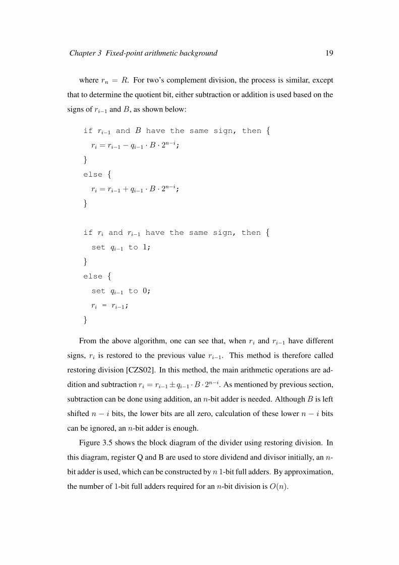
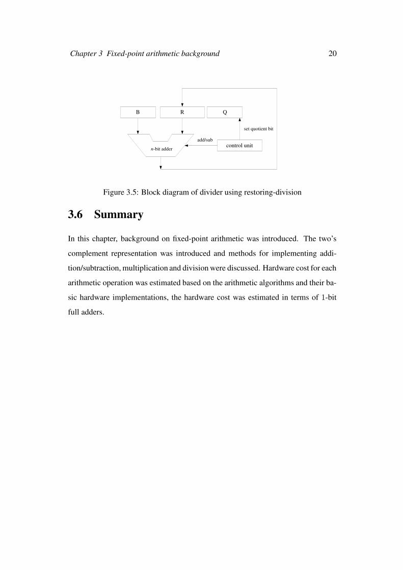
Figure 3.5 shows the block diagram of the divider using restoring division. In
this diagram, register Q and B are used to store dividend and divisor initially, an n-
bit adder is used, which can be constructed by n 1-bit full adders. By approximation,
the number of 1-bit full adders required for an n-bit division is O(n).
Chapter 3 Fixed-point arithmetic background 20
R
n -bit adder control unit
Q B
add/sub
set quotient bit
Figure 3.5: Block diagram of divider using restoring-division
3.6 Summary
In this chapter, background on fixed-point arithmetic was introduced. The two’s
complement representation was introduced and methods for implementing addi-
tion/subtraction, multiplication and division were discussed. Hardware cost for each
arithmetic operation was estimated based on the arithmetic algorithms and their ba-
sic hardware implementations, the hardware cost was estimated in terms of 1-bit
full adders.
Chapter 4
Fixed-point class implementation
4.1 Introduction
In order to analyze quantization effects of fixed-point arithmetic in fixed-point dig-
ital signal processing system, a fixed-point class, called Fixed, was developed to
simulate fixed-point arithmetic in the C++ language. All operands are Fixed type,
fixed-point calculated was handled internally by the fixed-point class. The detailed
implementation of the fixed-point class will be described in this chapter.
This chapter is organized as follows. Section 4.2 introduce how to use overload-
ing feature of the C++ language to simulate a fixed-point system. Some features
and implementation of the fixed-point class are presented in Section 4.3. The last
section is the summary.
4.2 Fixed-point simulation using overloading
In this work, we employ the simulation-based approach to analyze the quantization
effects associated with each variable and collect statistical information from each
variable during simulation. A fixed-point class, called Fixed, was developed to
achieve this goal. All operands in a fixed-point system are defined as Fixed, some
methods are implemented to handle the fixed-point arithmetic operations, such as
21
Chapter 4 Fixed-point class implementation 22
addition, subtraction, multiplication and division. In the following, an example will
be given to show how to use this fixed-point class to simulate fixed-point arithmetic.
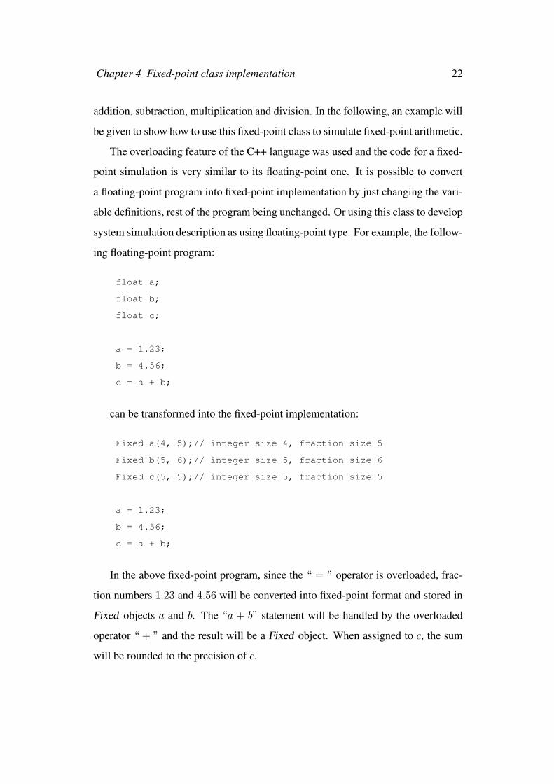
The overloading feature of the C++ language was used and the code for a fixed-
point simulation is very similar to its floating-point one. It is possible to convert
a floating-point program into fixed-point implementation by just changing the vari-
able definitions, rest of the program being unchanged. Or using this class to develop
system simulation description as using floating-point type. For example, the follow-
ing floating-point program:
float a;
float b;
float c;
a = 1.23;
b = 4.56;
c = a + b;
can be transformed into the fixed-point implementation:
Fixed a(4, 5);// integer size 4, fraction size 5
Fixed b(5, 6);// integer size 5, fraction size 6
Fixed c(5, 5);// integer size 5, fraction size 5
a = 1.23;
b = 4.56;
c = a + b;
In the above fixed-point program, since the “ = ” operator is overloaded, frac-
tion numbers 1.23 and 4.56 will be converted into fixed-point format and stored in
Fixed objects a and b. The “a + b” statement will be handled by the overloaded
operator “ + ” and the result will be a Fixed object. When assigned to c, the sum
will be rounded to the precision of c.
Chapter 4 Fixed-point class implementation 23
#include <stdio.h> #include <stdlib.h>
class Fixed { private: int IntegerSize; int FractionSize;
MY_FLOAT SingleMax; MY_FLOAT SingleMin;
MY_FLOAT ArrayMax; MY_FLOAT ArrayMin; int isArray; Fixed *arrayPtr;
MY_INT FixedValue; MY_FLOAT FloatValue;
public: //// constructor //// Fixed(int, int, MY_FLOAT); //// end constructor ////
//// return value//// MY_FLOAT getQerr(); int getIWL(); //// end return value////
//// for array use //// MY_INT setArray(Fixed *); //// end for array use ////
//// overload operator //// Fixed operator = (Fixed); Fixed operator = (const MY_FLOAT); Fixed operator + (Fixed ); Fixed operator - (Fixed ); Fixed operator * (Fixed ); Fixed operator / (Fixed ); //// end overload operator ////
//// calculate cos //// Fixed mcos(int, int); //// end calculate cos //// }
Figure 4.1: Fixed-point class declaration
Chapter 4 Fixed-point class implementation 24
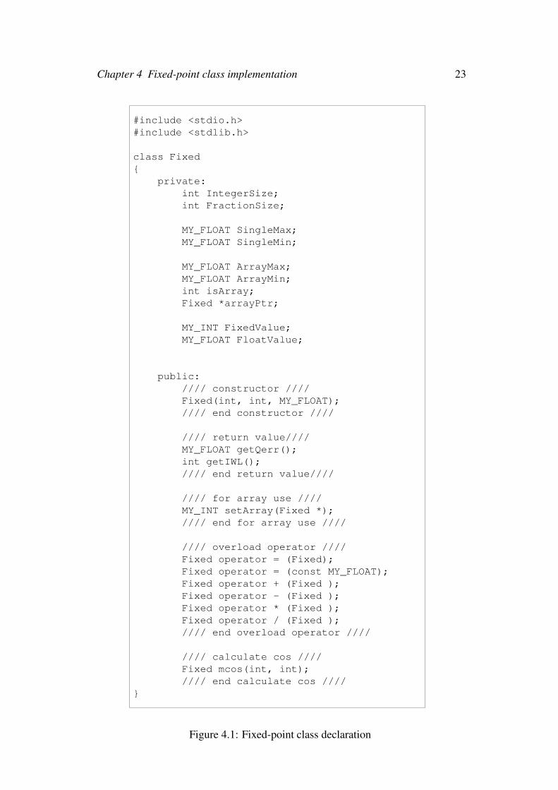
4.3 Fixed-point class implementation
Figure 4.1 shows the declaration of the fixed-point class. A fixed-point object is
defined to represent two’s complement fractions with arbitrary precision in fixed-
point format. Detailed implementation is introduced as follows.
4.3.1 Fixed-point object declaration
A fixed-point variable can be declared as:
Fixed VariableName;
Fixed VariableName (IntegerSize, FractionSize);
Fixed VariableName (IntegerSize, FractionSize, FloatingPointValue);
The parameters IntegerSize/FractionSize are used to define the integer/fraction
size of the fixed-point format in Figure 3.2 of the previous chapter. By defining
different IntegerSize and FractionSize for each object, all variables in a fixed-
point system can be of arbitrary wordlength. These two values are stored in the
private variables IntegerSize/FractionSize of the object as shown in Figure 4.1.
If IntegerSize/FractionSize is not specified when declaring a variable, default
values will be used.
The parameter F loatingPointV alue is stored in the private variableF loatV alue
of the object as shown in Figure 4.1 and FixedV alue will store the corresponding
fixed-point representation. In Figure 4.1, MY INT is a longlong type, which is
64-bit integer, used to simulate fixed-point format. MY FLOAT is a double type,
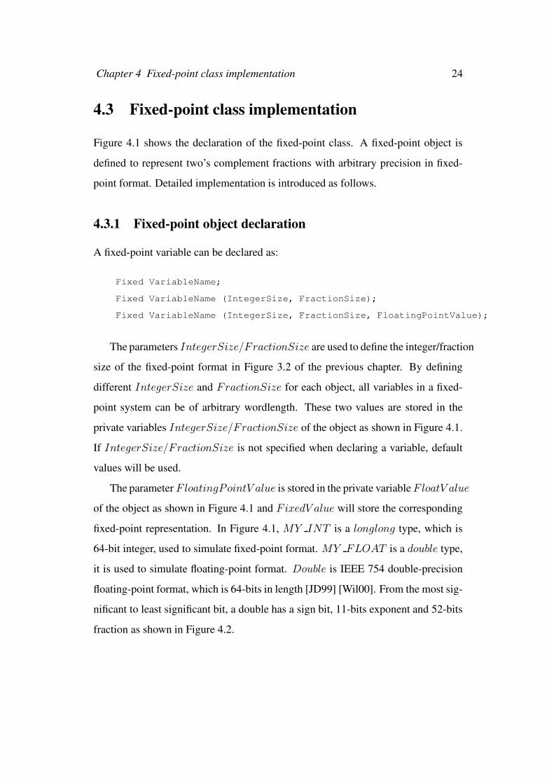
it is used to simulate floating-point format. Double is IEEE 754 double-precision
floating-point format, which is 64-bits in length [JD99] [Wil00]. From the most sig-
nificant to least significant bit, a double has a sign bit, 11-bits exponent and 52-bits
fraction as shown in Figure 4.2.
Chapter 4 Fixed-point class implementation 25
1
Sign Fraction
11 52
Exponent
64 bits
Figure 4.2: IEEE 754 double-precision format
4.3.2 Overload the operators
In order to overload the fixed-point operators, namely addition, subtraction, multi-
plication and division, corresponding methods were implemented in the fixed-point
class. The following shows the method signatures:
Fixed Fixed::operator + (Fixed) { implementation }
Fixed Fixed::operator - (Fixed) { implementation }
Fixed Fixed::operator * (Fixed) { implementation }
Fixed Fixed::operator / (Fixed) { implementation }
Fixed Fixed::operator = (const MY_FLOAT) { implementation }
Fixed Fixed::operator = (Fixed) { implementation }
Where “::” is called scope resolution operator, the notation “ClassName::MethodName”
means the method “MethodName” is belong to class “ClassName”. A mathematical
expression
C = A operator B (4.1)
can be regarded as
C = A.operator(B) (4.2)
and handled by corresponding methods. One can see that, all methods take a
Fixed object as input, and the returned result is also a Fixed object. Note that, the
Chapter 4 Fixed-point class implementation 26
FixedValu e
FloatValue FixedValu
e FloatValue
Fixed-point +, -, *, /
Floating-point +, -, *, /
FixedValu e
FloatValue
Operand A
Operand B
Operand C
Operator
Figure 4.3: Arithmetic calculation using fixed-point object
assignment operator is also overloaded. If the input operand is a fraction number,
this method will convert this fraction number into fixed-point format and stored in
the Fixed object at a precision specified by the target object. If the input is a Fixed
object, this method will round it to the target object’s precision.
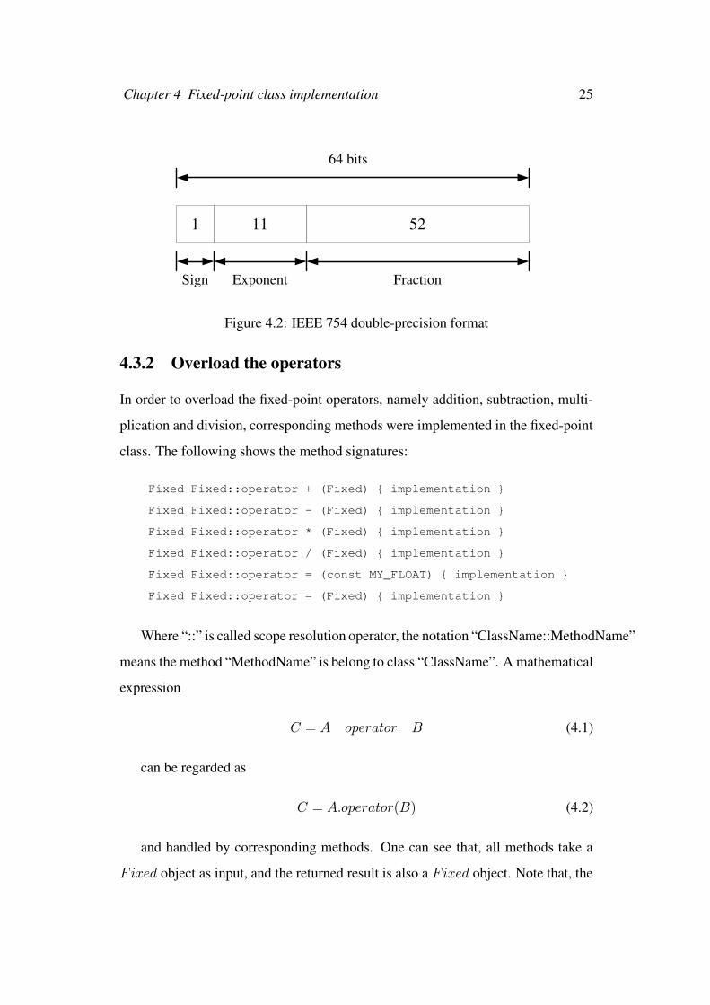
4.3.3 Arithmetic operations
The fixed-point class performs all calculations using both fixed-point and IEEE
754 double precision formats. The calculation result using fixed-point arithmetic
is stored in FixedValue, and the calculation result using floating-point arithmetic
is stored in FloatValue. This process can be shown by Figure 4.3. It is assumed
throughout this work that calculations done in double precision floating-point are
without error.
To avoid loss of precision during calculation, for addition, subtraction and di-
vision, the result use the maximum integer and fraction sizes of the two input
operands. For multiplication, the product’s wordlength is the summation of the two
input operands’ wordlengths minus one. This calculation result will be rounded to
Chapter 4 Fixed-point class implementation 27
the target operand’s precision when performing assignment operation by the over-
loaded “ = ” operator.
4.3.4 Automatic monitoring of dynamic range
During calculation, the fixed-point class can monitor the dynamic range of each
variable, and store the absolute maximum/minimum values in private variables
SingleMax/SingleMin. After each calculation, the absolute result is compared
with the existing maximum/minimum values. If it is larger than the maximum value,
it will be stored in SingleMax, on the other hand, it will be stored in SingleMin
if it is smaller than the minimum value. The minimum integer size of each variable
which guarantees that overflow will not occur, can be calculated from SingleMax
using the following equation
IntegerSize = int(log2 SingleMax) + 2; (4.3)
The minimum integer size required to represent the positive number SingleMax
is int(log2 SingleMax)+1. Since all numbers are using two’s complement format,
additional one bit is needed for the sign bit. As a result, int(log2 SingleMax) + 2
bits are required. A method, called getIWL(), is provided by this fixed-point class
to retrieve the minimum integer size.
4.3.5 Automatic calculation of quantization error
Since the fixed-point class performs operations using both fixed-point and floating-
point arithmetic, the quantization effects between fixed-point and floating-point
arithmetic are easily analyzed. Using the floating-point result as a reference, quan-
tization error is computed as follows
Qerr = 20∗ log
∣∣∣∣FixedV alue− F loatV alue
F loatV alue
∣∣∣∣. (4.4)
A method, called getQerr(), is implemented to get the quantization error of a
Fixed object.
Chapter 4 Fixed-point class implementation 28
4.3.6 Array supporting
The fixed-point class supports arrays, an array can be declared as follows
Fixed VariableName[NumberOfElements];
It can also be declared dynamically using malloc as follows
Fixed *VariableName;
VariableName = (Fixed *) malloc (sizeof(Fixed) * NumberOfElements);
In Figure 4.1, the private variable isArray is used to indicate whether this object
is an element of an array. ArrayMax/ArrayMin are used to store the absolute
maximum/minimum value of an array. Each array element has a pointer that point
to a Fixed object, the pointer address is stored in the private variable arrayP tr. If
any element’s value is updated,ArrayMax/ArrayMin of the Fixed object, which
is pointed by arrayP tr, will be updated if the updated value of this element is a
new maximum/minimum value of the entire array. As a result, after finishing all
fixed-point computation, ArrayMax/ArrayMin of the Fixed object pointed to
by arrayP tr will store the absolute maximum/minimum value of the entire array.
The method, setArray(Fixed∗), is used to save the pointer value to arrayP tr.
The minimum integer size of an array can be calculated as follows
IntegerSize = int(log2 ArrayMax) + 2; (4.5)
4.3.7 Cosine calculation
A method was implemented to compute the cosine function cos(2 ∗ π ∗ i/N). A
set of results for i from 0 to N were calculated using double precision format, for
a given input i, the double precision cosine result is converted into a fixed-point
format and stored in the Fixed object, note that it is rounded to the target operand’s
precision during conversion. From the application program’s point of view, it is a
look up table implementation of the cosine function. The following is the simplified
pseudo code:
Chapter 4 Fixed-point class implementation 29
Fixed Fixed::mcos(int i, int N)
{
cosResult = cos(2.0 * PI * i / N);
result = Fixed(this->IntegerSize, this->FractionSize, cosResult);
return result;
}
4.4 Summary
A fixed-point class is developed to simulated fixed-point arithmetic, overloading is
used, the fixed-point simulation program is very similar to a corresponding floating-
point description. In this chapter, some features and implementation, which are
convenient for quantization effect analysis, are introduced, e.g. automatic dynamic
range monitoring, automatic quantization error calculation. A look up table imple-
mentation of an cosine function was presented. This class was used to simulate
a fixed-point isolated word recognition system which will be introduced in a later
chapter.
Chapter 5
Speech recognition background
5.1 Introduction
To analyze the quantization effects in a non-trivial example, an isolated word recog-
nition system was studied. In this chapter, the isolated word recognition system is
introduced.
This chapter is organized as follows. An overview of the isolated word recogni-
tion system is presented in Section 5.2, the system is constructed based on the linear
predictive coding, vector quantization and hidden Markov model. Section 5.3 in-
troduce the linear predictive coding model applied in speech. In Section 5.4, vector
quantization is introduced while Section 5.5 explain the hidden Markov model used
to calculate the score of input speech. The last section is a summary.
5.2 Isolated word recognition system overview
There are many hardware implementations of isolated word recognition systems, ir-
respective of the implementations, trade-offs between performance and complexity
always exists. In order to get higher recognition accuracy, some complex models
can be used, on the other hand, simple models can be used, but the recognition ac-
curacy will be lower. In this section, the isolated word recognition system used in
this work will be introduced.
30
Chapter 5 Speech recognition background 31
LPC processor
VQ codebook for word 1
VQ codebook for word 4
VQ codebook for word 3
VQ codebook for word 2
HMM for word 1
HMM for word 4
HMM for word 3
HMM for word 2
Find Maximum
Score
speech data
output word
.
.
.
.
.
.
Figure 5.1: Isolated word recognition system
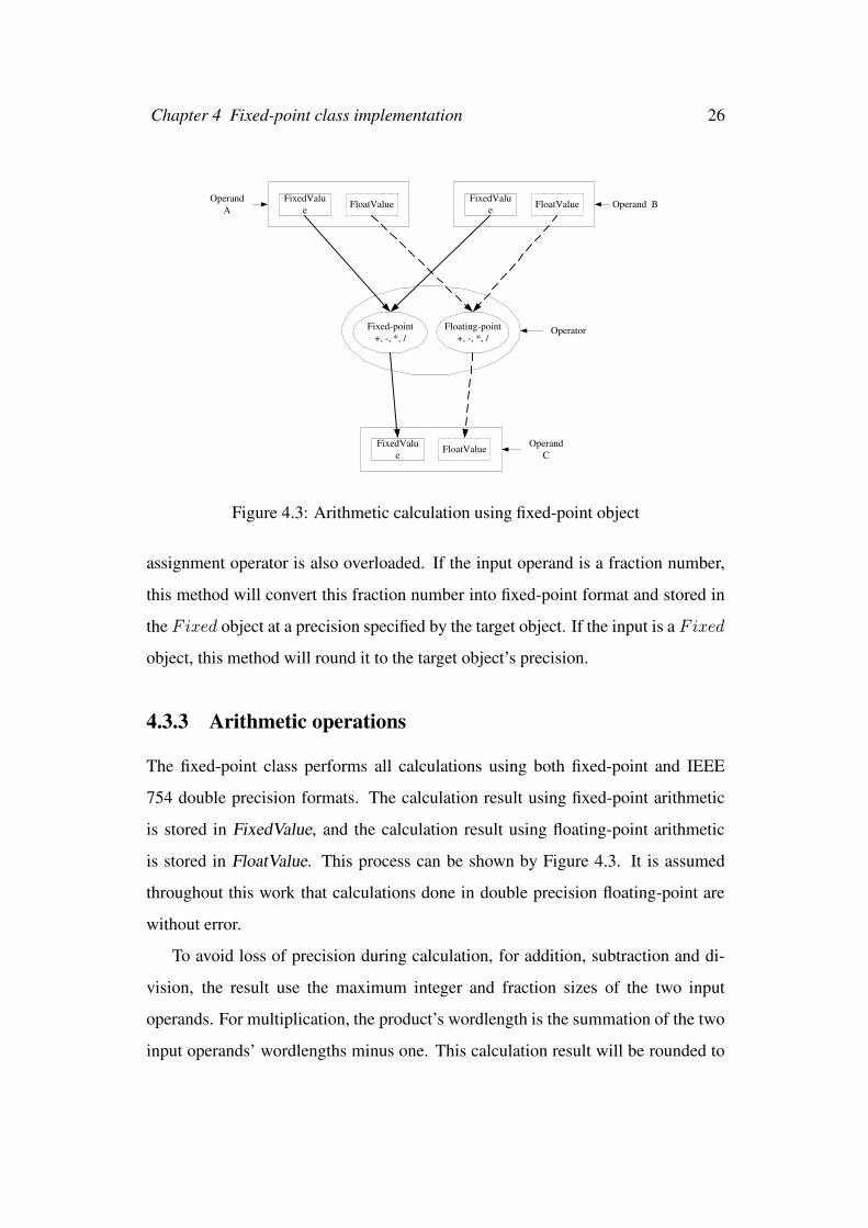
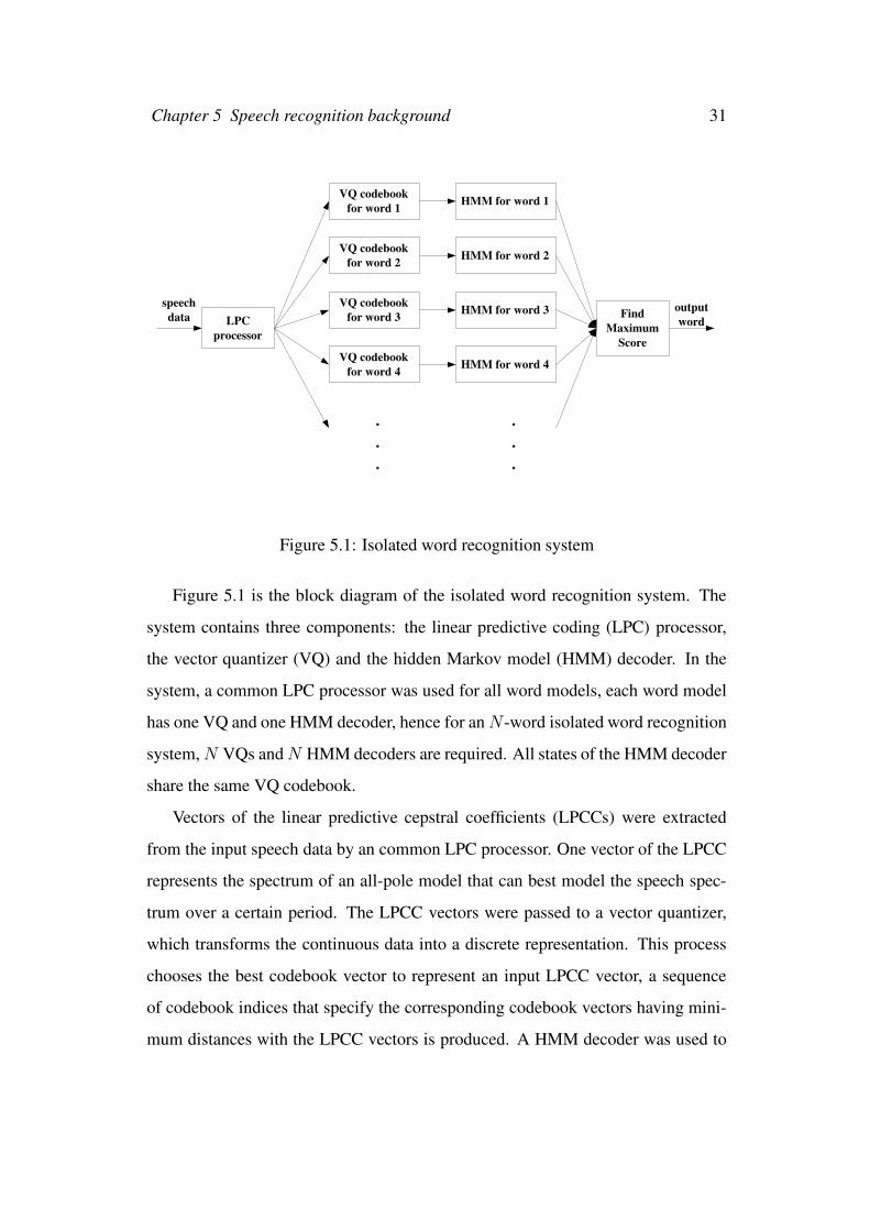
Figure 5.1 is the block diagram of the isolated word recognition system. The
system contains three components: the linear predictive coding (LPC) processor,
the vector quantizer (VQ) and the hidden Markov model (HMM) decoder. In the
system, a common LPC processor was used for all word models, each word model
has one VQ and one HMM decoder, hence for anN -word isolated word recognition
system,N VQs andN HMM decoders are required. All states of the HMM decoder
share the same VQ codebook.
Vectors of the linear predictive cepstral coefficients (LPCCs) were extracted
from the input speech data by an common LPC processor. One vector of the LPCC
represents the spectrum of an all-pole model that can best model the speech spec-
trum over a certain period. The LPCC vectors were passed to a vector quantizer,
which transforms the continuous data into a discrete representation. This process
chooses the best codebook vector to represent an input LPCC vector, a sequence
of codebook indices that specify the corresponding codebook vectors having mini-
mum distances with the LPCC vectors is produced. A HMM decoder was used to
Chapter 5 Speech recognition background 32
calculate the score for the vector quantizer’s output sequence. For an isolated word
recognition system containing N words, N scores will be obtained and the word
with the maximum score is chosen as the output word. The detailed background
of the LPC processor, VQ and HMM decoder will be introduced in the following
sections.
5.3 Linear predictive coding processor
Linear predictive coding (LPC) theory has been used in speech recognition sys-
tem for many years, a large number of recognizers were constructed based on LPC
theory. It is because LPC has the following advantages:
1. LPC provides a good approximation to speech signal, it is more effective for
voiced regions, and acceptable for unvoiced regions [LB93].
2. The mathematical calculation in LPC is simple, and is suitable for both soft-
ware and hardware implementations.
In the past, due to the limitation of hardware technology, reaching real time
performance was very difficult, and the second point made it easier to reach real
time performance.
5.3.1 The LPC model
In an LPC model, speech sample s(m) at time m can be approximated as a linear
combination of the previous t speech samples:
s(m) =t∑
n=1
ans(m− n) +Gu(m) (5.1)
where Gu(m) is an excitation term. Transformed into the z-domain, we obtain the
transfer function:
H(z) =1
1−∑tn=1 anz
−n . (5.2)
Chapter 5 Speech recognition background 33
�
=−− t
n
nn za
11 �⊗⊗⊗⊗�
s(m)�
gain(G)�
u(m)�
Figure 5.2: LPC model of speech
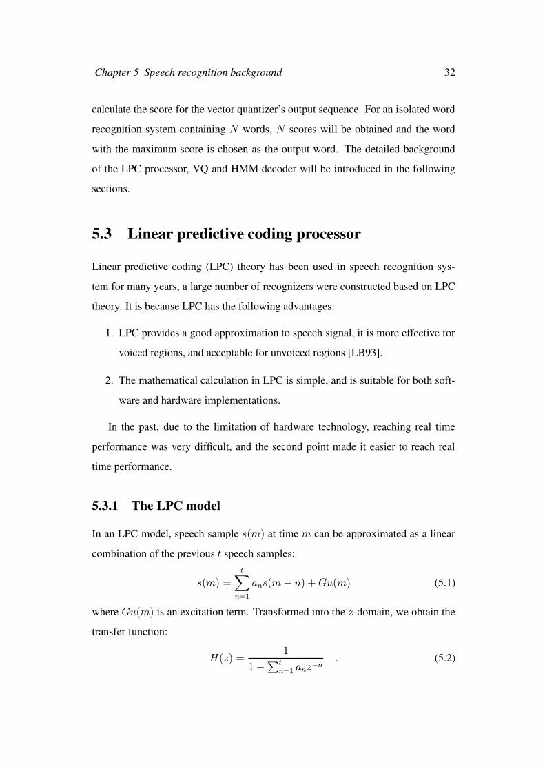
As shown in Figure 5.2, the normalized excitation source u(m) is scaled by the
gain G. In speech recognition, the LPC feature analysis finds the filter coefficients
an that can best model the speech data, which are used for further processing in the
recognition process. It is noted that, the higher the filter order, the better the spoken
sounds it can model.
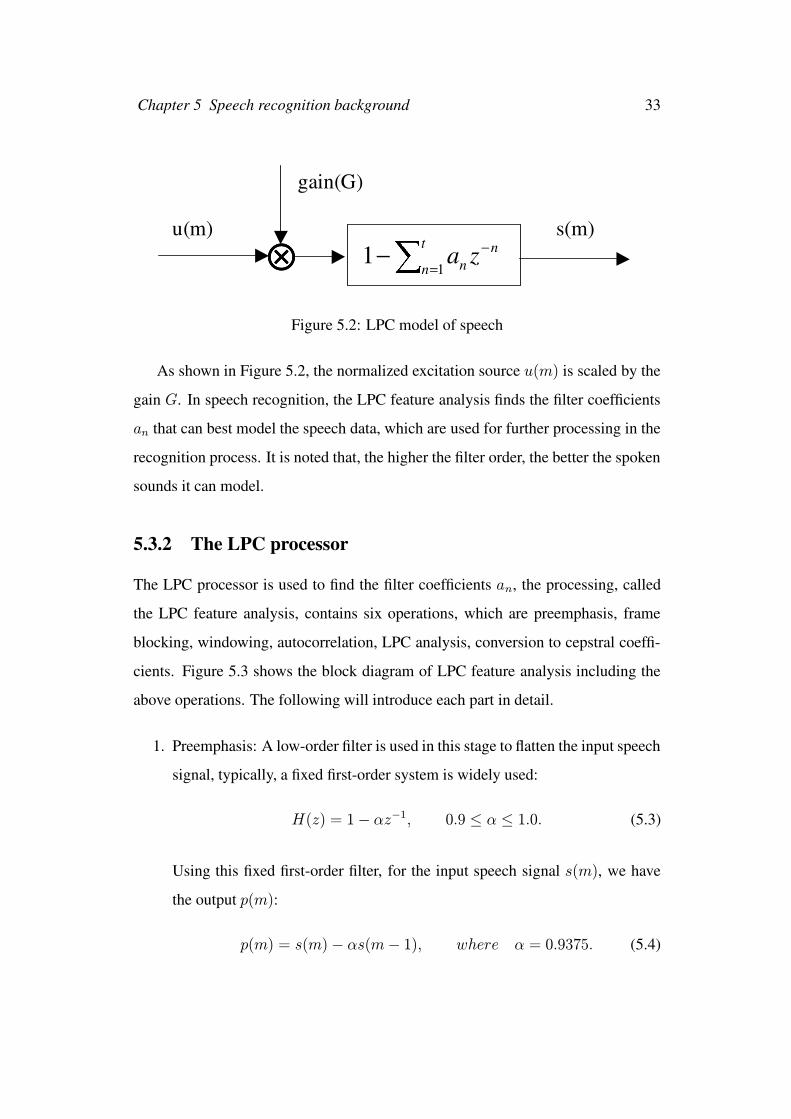
5.3.2 The LPC processor
The LPC processor is used to find the filter coefficients an, the processing, called
the LPC feature analysis, contains six operations, which are preemphasis, frame
blocking, windowing, autocorrelation, LPC analysis, conversion to cepstral coeffi-
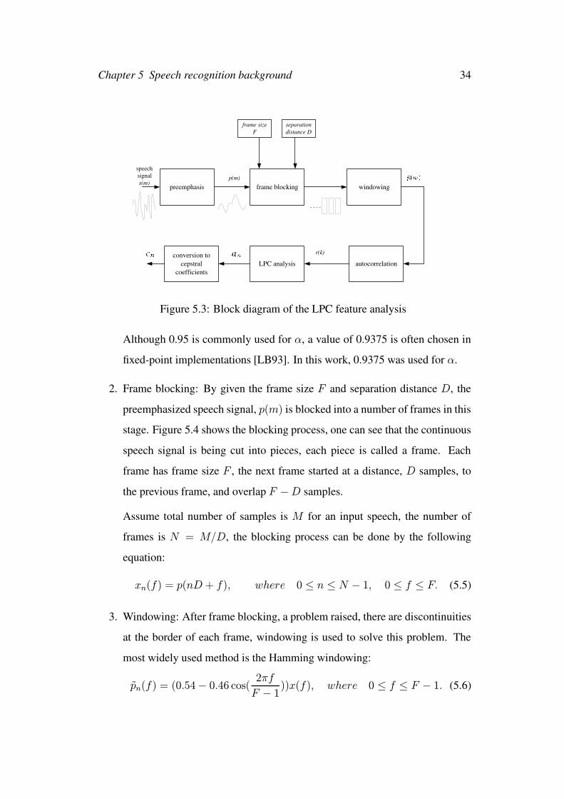
cients. Figure 5.3 shows the block diagram of LPC feature analysis including the
above operations. The following will introduce each part in detail.
1. Preemphasis: A low-order filter is used in this stage to flatten the input speech
signal, typically, a fixed first-order system is widely used:
H(z) = 1− αz−1, 0.9 ≤ α ≤ 1.0. (5.3)
Using this fixed first-order filter, for the input speech signal s(m), we have
the output p(m):
p(m) = s(m)− αs(m− 1), where α = 0.9375. (5.4)
Chapter 5 Speech recognition background 34
preemphasis frame blocking windowing
autocorrelation LPC analysis conversion to
cepstral coefficients
speech signal s(m)
p(m )
r(k )
separation distance D
frame size F
....
Figure 5.3: Block diagram of the LPC feature analysis
Although 0.95 is commonly used for α, a value of 0.9375 is often chosen in
fixed-point implementations [LB93]. In this work, 0.9375 was used for α.
2. Frame blocking: By given the frame size F and separation distance D, the
preemphasized speech signal, p(m) is blocked into a number of frames in this
stage. Figure 5.4 shows the blocking process, one can see that the continuous
speech signal is being cut into pieces, each piece is called a frame. Each
frame has frame size F , the next frame started at a distance, D samples, to
the previous frame, and overlap F −D samples.
Assume total number of samples is M for an input speech, the number of
frames is N = M/D, the blocking process can be done by the following
equation:
xn(f) = p(nD + f), where 0 ≤ n ≤ N − 1, 0 ≤ f ≤ F. (5.5)
3. Windowing: After frame blocking, a problem raised, there are discontinuities
at the border of each frame, windowing is used to solve this problem. The
most widely used method is the Hamming windowing:
pn(f) = (0.54− 0.46 cos(2πf
F − 1))x(f), where 0 ≤ f ≤ F − 1. (5.6)
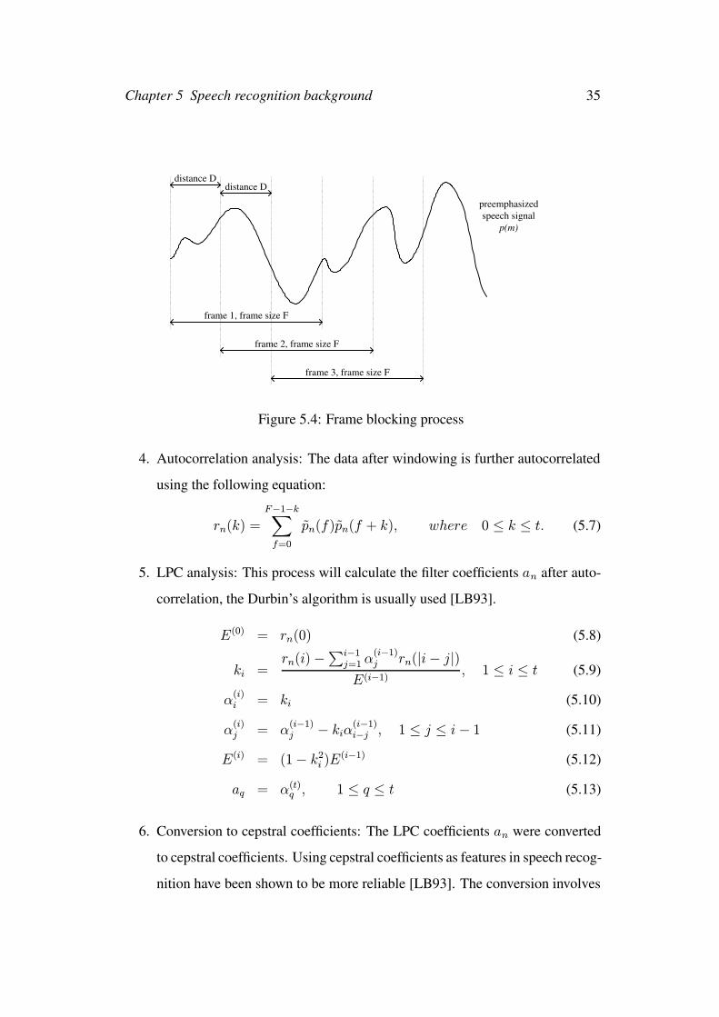
Chapter 5 Speech recognition background 35
frame 1, frame size F
frame 2, frame size F
frame 3, frame size F
distance D distance D
preemphasized speech signal
p(m)
Figure 5.4: Frame blocking process
4. Autocorrelation analysis: The data after windowing is further autocorrelated
using the following equation:
rn(k) =F−1−k∑
f=0
pn(f)pn(f + k), where 0 ≤ k ≤ t. (5.7)
5. LPC analysis: This process will calculate the filter coefficients an after auto-
correlation, the Durbin’s algorithm is usually used [LB93].
E(0) = rn(0) (5.8)
ki =rn(i)−∑i−1
j=1 α(i−1)j rn(|i− j|)
E(i−1), 1 ≤ i ≤ t (5.9)
α(i)i = ki (5.10)
α(i)j = α
(i−1)j − kiα(i−1)
i−j , 1 ≤ j ≤ i− 1 (5.11)
E(i) = (1− k2i )E
(i−1) (5.12)
aq = α(t)q , 1 ≤ q ≤ t (5.13)
6. Conversion to cepstral coefficients: The LPC coefficients an were converted
to cepstral coefficients. Using cepstral coefficients as features in speech recog-
nition have been shown to be more reliable [LB93]. The conversion involves
Chapter 5 Speech recognition background 36
c(1)
c(3)
c(4)
c(2)
v(1)
codebook
.
.
.
.
v(3) v(2) . . .
Find minimum distance
Calculate distance between each input
vector and each codebook vector
i(1) i(3) i(2) . . .
codebook indices input vectors
Figure 5.5: Vector quantization process
the following calculations:
cn = an +n−1∑
k=1
(k
n)ckan−k, where 1 ≤ n ≤ t. (5.14)
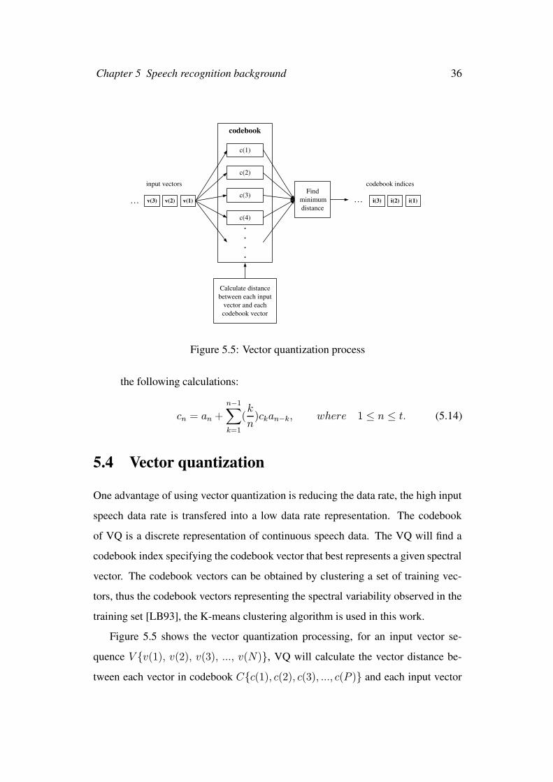
5.4 Vector quantization
One advantage of using vector quantization is reducing the data rate, the high input
speech data rate is transfered into a low data rate representation. The codebook
of VQ is a discrete representation of continuous speech data. The VQ will find a
codebook index specifying the codebook vector that best represents a given spectral
vector. The codebook vectors can be obtained by clustering a set of training vec-
tors, thus the codebook vectors representing the spectral variability observed in the
training set [LB93], the K-means clustering algorithm is used in this work.
Figure 5.5 shows the vector quantization processing, for an input vector se-
quence V {v(1), v(2), v(3), ..., v(N)}, VQ will calculate the vector distance be-
tween each vector in codebook C{c(1), c(2), c(3), ..., c(P )} and each input vector
Chapter 5 Speech recognition background 37
v(n), and the codebook index with minimum distance will be chosen as output. Af-
ter vector quantization, a sequence of codebook indices I{i(1), i(2), i(3), ..., i(N)}will be produced.
The vector distance between an input vector v(n) and each vector in codebook
is calculated using:
d(v(i), c(j)) =K∑
k=1
[v(i)(k)− c(j)(k)]2, (5.15)
where v(i)(k) is the kth element of the input vector v(i), c(i)(k) is the kth element
of the codebook vector c(i), K is the vector length. The following is the pseudo
code for vector quantization.
for p from 1 to codebook size {distance(p) = 0;
for k from 1 to vector length {temp = (v(n)(k) - c(p)(k))*(v(n)(k) - c(p)(k));
distance(p) = distance(p) + temp;
}}i(n) = arg minp (distance(p));
In the above pseudo code, i(n) is the nth element of the output codebook indices
sequence as shown in Figure 5.5. Similar input vectors are clustered together in
vector quantization, one can see that the data rate is reduced significantly. This
advantage will benefit most HMM based speech recognition system using vector
quantization, because HMM decoding is time consuming, lower data rate will make
real time performance become realizable in the past. Furthermore, the storage size
is reduced for spectral analysis data, only the codebook will be stored, as a result, it
is more suitable for hardware implementation.
Chapter 5 Speech recognition background 38
S0 S1 S2
a 00 a 22
a 12
a 11
a 01
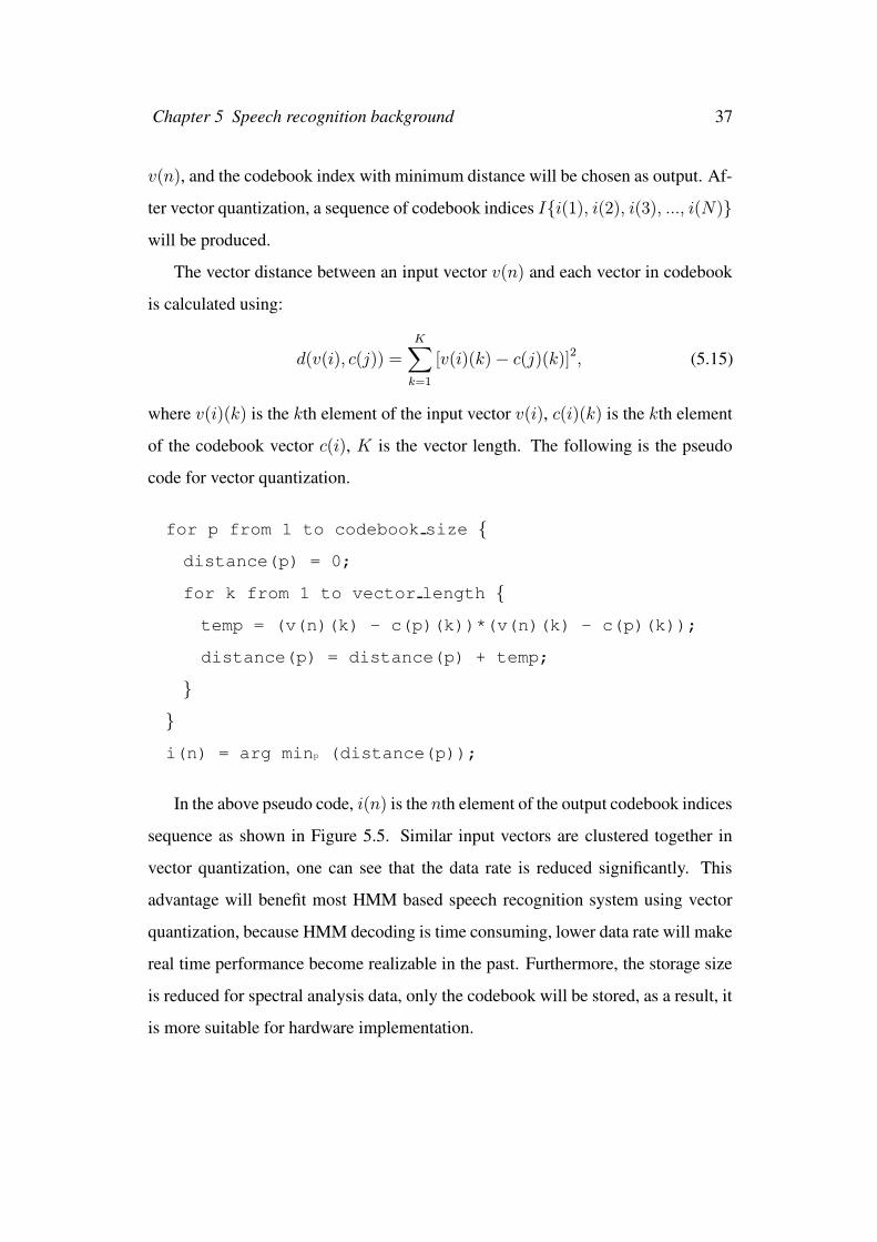
Figure 5.6: Left-to-Right HMM
5.5 Hidden Markov model
Hidden Markov models (HMMs) are widely used in modern speech recognition
systems because HMM-based speech recognition systems have proven to yield high
recognition accuracy. The Viterbi algorithm is used to find the most likely state
sequence and likehood score for a given observation sequence. In this section, the
background theory of HMM and the Viterbi algorithm will be introduced.
Given an observation sequence O = (o1o2...oT ), HMM decoding calculates
P (O|λ), which is the probability of the input observation sequence for a given
model λ, the result means how much chance the utterance represented by model
λ will produce the observation sequence O.
Figure 5.6 shows a basic three-state left-to-right HMM. A HMM is a proba-
bilistic finite state machine (FSM) and has a set of state transaction and observation
probabilities. The state transaction probability is the probability of state transaction
from one to another, and the observation probability is the probability that a state
emit a particular observation. In this figure, S0, S1, S2 are the states, aij is the
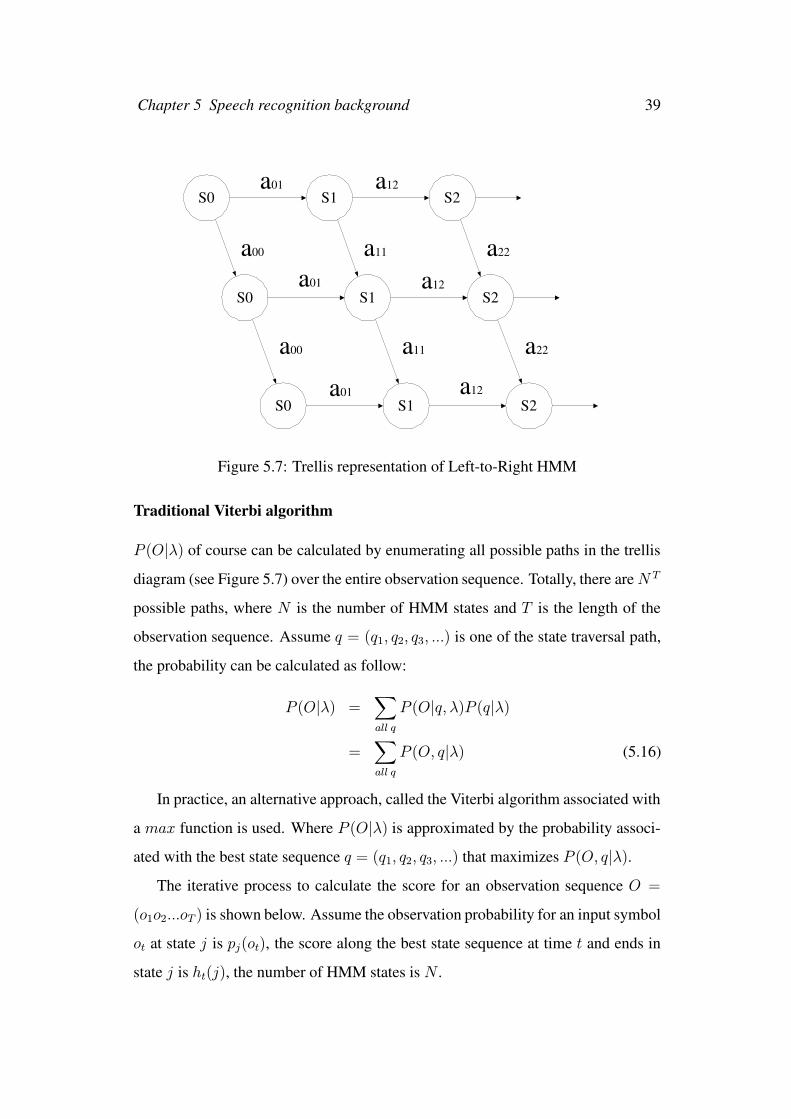
probability of state transaction from i to j. Figure 5.7 is the trellis representation
showing all possible state transaction paths.
Chapter 5 Speech recognition background 39
S0 S1 S2
S0 S1 S2
S0 S1 S2
a 12 a 01
a 01
a 22 a 11 a 00
a 22 a 11 a 00
a 12
a 12 a 01
Figure 5.7: Trellis representation of Left-to-Right HMM
Traditional Viterbi algorithm
P (O|λ) of course can be calculated by enumerating all possible paths in the trellis
diagram (see Figure 5.7) over the entire observation sequence. Totally, there areN T
possible paths, where N is the number of HMM states and T is the length of the
observation sequence. Assume q = (q1, q2, q3, ...) is one of the state traversal path,
the probability can be calculated as follow:
P (O|λ) =∑
all q
P (O|q, λ)P (q|λ)
=∑
all q
P (O, q|λ) (5.16)
In practice, an alternative approach, called the Viterbi algorithm associated with
a max function is used. Where P (O|λ) is approximated by the probability associ-
ated with the best state sequence q = (q1, q2, q3, ...) that maximizes P (O, q|λ).
The iterative process to calculate the score for an observation sequence O =
(o1o2...oT ) is shown below. Assume the observation probability for an input symbol
ot at state j is pj(ot), the score along the best state sequence at time t and ends in
state j is ht(j), the number of HMM states is N .
Chapter 5 Speech recognition background 40
1. Looping:
ht(j) = max1≤i≤N
[ht−1(i)aij]pj(ot) (5.17)
2. Stop:
H = max1≤i≤N
[hT (i)] (5.18)
By using the max function, calculation can be reduced. But since multiplica-
tion is performed for each iteration, underflow problem may occur, an alternative
approach is introduced.
Alternative Viterbi approach
To overcome the underflow problem, taking logarithms in Equation 5.17, results in
the following procedures:
1. Looping:
ht(j) = max1≤i≤N
[ht−1(i) + aij] + pj(ot) (5.19)
2. Stop:
H = max1≤i≤N
[hT (i)] (5.20)
Using this approach, computation is reduced since the main operations are ad-
dition rather than multiplication. This approach is very suitable for hardware im-
plementation, and was adopted in this work.
5.6 Summary
Background of an isolated word recognition system was introduced in this chapter.
The isolated word recognition consists of the LPC processor, VQ and HMM de-
coder using the Viterbi algorithm, the output of HMM decoder are the word scores,
and the highest is taken to be the recognized word.
Chapter 6
Optimization
6.1 Introduction
To perform wordlength optimization of fixed-point system, one difficulty is that,
the objective function cannot be stated as explicit functions of the design variables
for most of implementations. For example, in speech recognition, the recognition
accuracy cannot be stated in terms of wordlength. As a result, traditional analytical
methods is difficult to be applied to all systems and a simulation searching-based
method can be used. The cost is obtained through simulation, and a searching
method is applied to find the optimal solution.
This chapter is organized as follows. In Section 6.2, the simplex method is
introduced. Section 6.3 present the one-dimensional optimization approach, which
significantly reduces the search space. Section 6.4 is a summary.
6.2 Simplex Method
The Nelder-Mead simplex method [JR65], published in 1965, is widely used in non-
linear unconstrained optimization. The Nelder-Mead method attempts to minimize
an object function of n variables, the minimization process depends on the function
value, no derivative information is required, the Nelder-Mead thus was classed as
41
Chapter 6 Optimization 42
direct search method [Sin96]. Because of these features, it can be regarded as a
general optimization method for wordlengths optimization in fixed-point systems.
In simplex method, a set of n + 1 initial point is formed for n-dimensional
space, then reflection, expansion and contraction process are applied to find optimal
solution.
6.2.1 Initialization
At the beginning, the user should supply a base point and guess scale. A set of n+1
initial point is generated using the following equations:
X0 = Xu (6.1)
Xi = Xu + pui, i = 1, 2, ..., n (6.2)
In the above equations, Xu is the base point and p is the guess scale, ui is the
unit vector along the ith coordinate axis. In the geometric figure’s point of view, the
n + 1 initial points formed is called a simplex.
For example, if X0 = [4, 5, 6] and p = 2, the initial points are:
X0 = Xu = [4, 5, 6]
X1 = Xu + pu1 = [6, 5, 6]
X2 = Xu + pu2 = [4, 7, 6]
X3 = Xu + pu3 = [4, 5, 8]
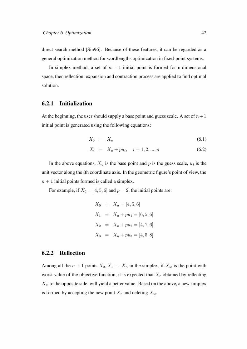
6.2.2 Reflection
Among all the n + 1 points X0, X1, ..., Xn in the simplex, if Xw is the point with
worst value of the objective function, it is expected that Xr obtained by reflecting
Xw to the opposite side, will yield a better value. Based on the above, a new simplex
is formed by accepting the new point Xr and deleting Xw.
Chapter 6 Optimization 43
X 0 X 1
X 2
X 3
X c
X 4
Figure 6.1: Reflection
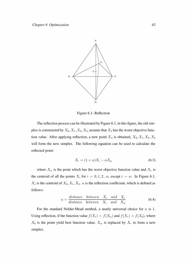
The reflection process can be illustrated by Figure 6.1, in this figure, the old sim-
plex is constructed byX0, X1, X2, X3, assume thatX3 has the worst objective func-
tion value. After applying reflection, a new point X4 is obtained, X0, X1, X2, X4
will form the new simplex. The following equation can be used to calculate the
reflected point:
Xr = (1 + α)Xc − αXw (6.3)
where Xw is the point which has the worst objective function value and Xc is
the centroid of all the points Xi for i = 0, 1, 2...n, except i = w. In Figure 6.1,
Xc is the centroid of X0, X1, X2. α is the reflection coefficient, which is defined as
follows:
α =distance between Xc and Xr
distance between Xc and Xw
(6.4)
For the standard Nelder-Mead method, a nearly universal choice for α is 1.
Using reflection, if the function value f(Xr) < f(Xw) and f(Xr) > f(Xb), where
Xb is the point yield best function value, Xw is replaced by Xr to form a new
simplex.
Chapter 6 Optimization 44
6.2.3 Expansion
Using reflection, if f(Xr) < f(Xb), it is expected that a point which has a better
function value can be obtained if we move along the direction pointing from Xc to
Xr. A new point Xe, obtained by further expand Xr in the direction pointing from
Xc to Xr, will be used to test the function value, this is called expansion. Xe can be
obtained using the following equation:
Xe = βXr + (1− β)Xc (6.5)
β is the expansion coefficient, which is defined as follows:
β =distance between Xc and Xe
distance between Xc and Xr
(6.6)
One can see that β must be larger than 1, for standard Nelder-Mead method, a
good choice is 2.
If the expansion point is a new best point, that means f(Xe) < f(Xb), Xw is
replaced by Xe and the reflection process will restart again. Otherwise, if f(Xe) >
f(Xb), Xw is replaced by Xr, and the reflection process is restarted.
6.2.4 Contraction
After reflection, Xw will be replaced by Xr if the following two conditions are
satisfied for a reflection point Xr:
(1) f(Xr) > f(Xi), where i = 0, 1, 2, ..., n, i 6= w
(2) f(Xr) < f(Xw)
Xw will remain unchanged if only the following condition satisfy for a reflection
point Xr:
f(Xr) > f(Xw)
Chapter 6 Optimization 45
Contraction is then applied to contract the simplex, a new point, generated using
the following equation, will be used to test the objective function.
Xt = γXw + (1− γ)Xc (6.7)
where γ is the contraction coefficient, which is defined as follows:
γ =distance between Xc and Xt
distance between Xc and Xw(6.8)
For standard Nelder-Mead method, γ is usually set to 12. The reflection process
will be restarted depending on the function value f(Xt) as follows:
• f(Xt) < min[f(Xr), f(Xw)]: That means the contraction was a success,
replace Xw by Xt, and restart the reflection process.
• f(Xt) ≥ min[f(Xr), f(Xw)]: Contraction is a failure, for i = 0, 1, 2, ..., n,
replace Xi by (Xi +Xb)/2, and restart the contraction.
6.2.5 Stop
The reflection process will stop if the number of iterations reaches a maximum
number, or if the following condition is satisfied:
2× | f(Xw)− f(Xb) || f(Xw) | + | f(Xb) |
< ε (6.9)
where ε is an user defined tolerance.
6.3 One-dimensional optimization approach
When performing wordlength optimization, one difficulty is that, the search space
is very large. To overcome this problem, instead of optimizing global system, each
variable is exhaustively searched between given bounds independently, which will
Chapter 6 Optimization 46
result in search space reduction. This is a trade-off between accuracy and execu-
tion time. The one-dimensional optimization approach may get trapped in a local
minima.
6.3.1 One-dimensional optimization approach
Detailed implementation of one-dimensional optimization approach can be summa-
rized as the following pseudo code, for a system consist of n variablesX1, X2, X3, ..., Xn,
each variable has a wordlength search space bound [L(i), U(i)] for i = 1, 2, 3, ..., n,
where L(i) is the lower bound of Xi and U(i) is the upper bound of Xi.
\\ Initialization
For i = 1 to n {WordLength(i) = U(i);
}
MinFunctionValue = f(U(1), U(2), U(3), ..., U(n));
\\ Minimize each variable alternatively
For i = 1 to n {\\ Sweep wordlength of Xi
For WordLength(i) = U(i) to L(i) {CurrentFunctionValue = f(WordLength(1), WordLength(2), ..., WordLength(n));
\\ Store the minimum wordlength
if CurrentFunctionValue < MinFunctionValue then {MinFunctionValue = CurrentFunctionValue;
MinWordLength(i) = WordLength(i);
}}WordLength(i) = MinWordLength(i);
}
In the above pseudo code, MinWordLength(i) is the minimum wordlength of
Xi.
The one-dimensional optimization can be illustrated by Figure 6.2, assume a
system consist of three variables X1, X2, X3, the optimization process is broken
into three parts. From the left to the right, suboptimize the wordlength of X1, X2
andX3 in sequence. When optimizing the wordlength of one variable, the others are
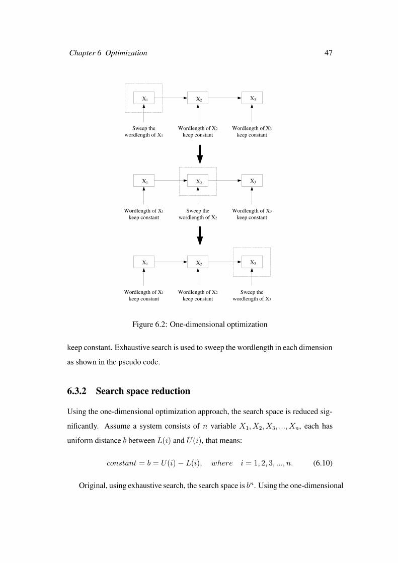
Chapter 6 Optimization 47
X 1 X 2 X 3
Sweep the wordlength of X 1
Wordlength of X 2
keep constant Wordlength of X 3
keep constant
X 1 X 2 X 3
Wordlength of X 1
keep constant Sweep the
wordlength of X 2
Wordlength of X 3
keep constant
X 1 X 2 X 3
Wordlength of X 1
keep constant Wordlength of X 2
keep constant Sweep the
wordlength of X 3
Figure 6.2: One-dimensional optimization
keep constant. Exhaustive search is used to sweep the wordlength in each dimension
as shown in the pseudo code.
6.3.2 Search space reduction
Using the one-dimensional optimization approach, the search space is reduced sig-
nificantly. Assume a system consists of n variable X1, X2, X3, ..., Xn, each has
uniform distance b between L(i) and U(i), that means:
constant = b = U(i)− L(i), where i = 1, 2, 3, ..., n. (6.10)
Original, using exhaustive search, the search space is bn. Using the one-dimensional
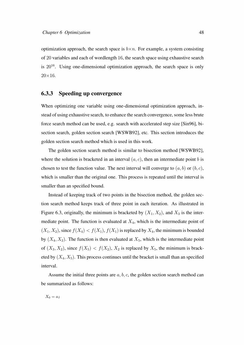
Chapter 6 Optimization 48
optimization approach, the search space is b×n. For example, a system consisting
of 20 variables and each of wordlength 16, the search space using exhaustive search
is 2016. Using one-dimensional optimization approach, the search space is only
20×16.
6.3.3 Speeding up convergence
When optimizing one variable using one-dimensional optimization approach, in-
stead of using exhaustive search, to enhance the search convergence, some less brute
force search method can be used, e.g. search with accelerated step size [Sin96], bi-
section search, golden section search [WSWB92], etc. This section introduces the
golden section search method which is used in this work.
The golden section search method is similar to bisection method [WSWB92],
where the solution is bracketed in an interval (a, c), then an intermediate point b is
chosen to test the function value. The next interval will converge to (a, b) or (b, c),
which is smaller than the original one. This process is repeated until the interval is
smaller than an specified bound.
Instead of keeping track of two points in the bisection method, the golden sec-
tion search method keeps track of three point in each iteration. As illustrated in
Figure 6.3, originally, the minimum is bracketed by (X1, X2), and X3 is the inter-
mediate point. The function is evaluated at X4, which is the intermediate point of
(X1, X2), since f(X4) < f(X1), f(X1) is replaced byX4, the minimum is bounded
by (X4, X2). The function is then evaluated at X5, which is the intermediate point
of (X3, X2), since f(X5) < f(X2), X2 is replaced by X5, the minimum is brack-
eted by (X4, X5). This process continues until the bracket is small than an specified
interval.
Assume the initial three points are a, b, c, the golden section search method can
be summarized as follows:
X0 = a;
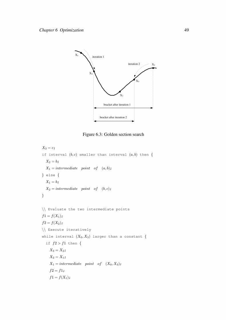
Chapter 6 Optimization 49
X 1
X 2
X 3
X 4
X 5
iteration 1
iteration 2
bracket after iteration 1
bracket after iteration 2
Figure 6.3: Golden section search
X3 = c;
if interval (b, c) smaller than interval (a, b) then {X2 = b;
X1 = intermediate point of (a, b);
} else {X1 = b;
X2 = intermediate point of (b, c);
}
\\ Evaluate the two intermediate points
f1 = f(X1);
f2 = f(X2);
\\ Execute iteratively
while interval (X0, X3) larger than a constant {if f2 > f1 then {X3 = X2;
X2 = X1;
X1 = intermediate point of (X0, X3);
f2 = f1;
f1 = f(X1);
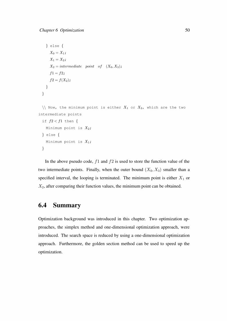
Chapter 6 Optimization 50
} else {X0 = X1;
X1 = X2;
X2 = intermediate point of (X0, X3);
f1 = f2;
f2 = f(X2);
}}
\\ Now, the minimum point is either X1 or X2, which are the two
intermediate points
if f2 < f1 then {Minimum point is X2;
} else {Minimum point is X1;
}
In the above pseudo code, f1 and f2 is used to store the function value of the
two intermediate points. Finally, when the outer bound (X0, X3) smaller than a
specified interval, the looping is terminated. The minimum point is either X1 or
X2, after comparing their function values, the minimum point can be obtained.
6.4 Summary
Optimization background was introduced in this chapter. Two optimization ap-
proaches, the simplex method and one-dimensional optimization approach, were
introduced. The search space is reduced by using a one-dimensional optimization
approach. Furthermore, the golden section method can be used to speed up the
optimization.
Chapter 7
Word Recognition System Design
Methodology
7.1 Introduction
A framework was introduced to address the quantization issues of fixed-point sys-
tems, flexibility and easy to be extensible are the major consideration of this frame-
work. It is applied to an isolated word recognition system to explore the utility of
this approach. In this chapter, detailed design of the framework is introduced.
This chapter is organized as follows. In Section 7.2, the architecture of frame-
work is introduced. Section 7.3 present how to apply this framework to an isolated
word recognition system. The last section is a summary.
7.2 Framework design
Figure 7.1 shows the block diagram of the framework, which consists of a fixed-
point class and an optimizer. Fixed-point application is simulated using the fixed-
point class, and the optimizer is used to find optimal wordlength.
51
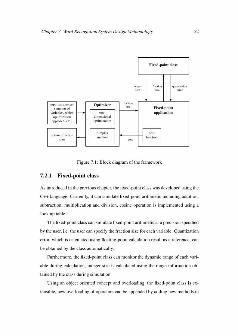
Chapter 7 Word Recognition System Design Methodology 52
one- dimensional optimization
Simplex method
Optimizer
cost function
Fixed-point application
Fixed-point class
fraction size
integer size
fraction size
quantization error
cost
input parameters (number of
variables, which optimization
approach, etc.)
optimal fraction size
Figure 7.1: Block diagram of the framework
7.2.1 Fixed-point class
As introduced in the previous chapter, the fixed-point class was developed using the
C++ language. Currently, it can simulate fixed-point arithmetic including addition,
subtraction, multiplication and division, cosine operation is implemented using a
look up table.
The fixed-point class can simulate fixed-point arithmetic at a precision specified
by the user, i.e. the user can specify the fraction size for each variable. Quantization
error, which is calculated using floating-point calculation result as a reference, can
be obtained by the class automatically.
Furthermore, the fixed-point class can monitor the dynamic range of each vari-
able during calculation, integer size is calculated using the range information ob-
tained by the class during simulation.
Using an object oriented concept and overloading, the fixed-point class is ex-
tensible, new overloading of operators can be appended by adding new methods in
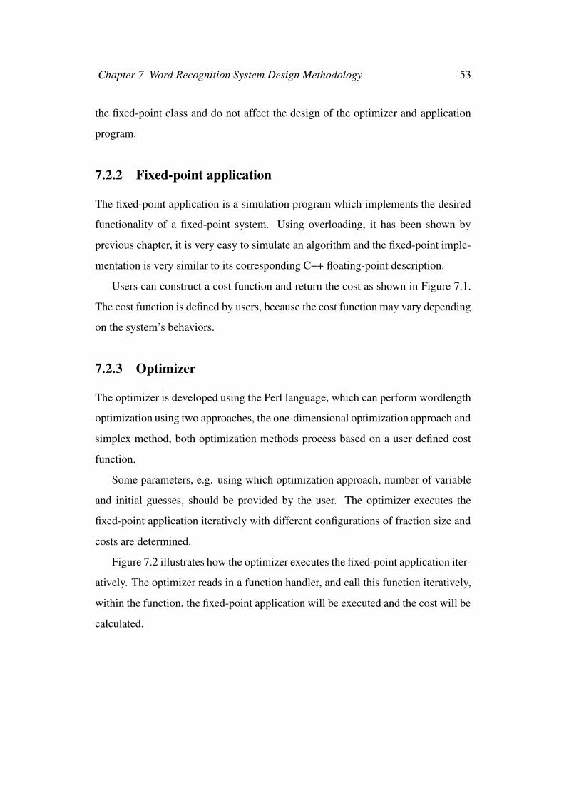
Chapter 7 Word Recognition System Design Methodology 53
the fixed-point class and do not affect the design of the optimizer and application
program.
7.2.2 Fixed-point application
The fixed-point application is a simulation program which implements the desired
functionality of a fixed-point system. Using overloading, it has been shown by
previous chapter, it is very easy to simulate an algorithm and the fixed-point imple-
mentation is very similar to its corresponding C++ floating-point description.
Users can construct a cost function and return the cost as shown in Figure 7.1.
The cost function is defined by users, because the cost function may vary depending
on the system’s behaviors.
7.2.3 Optimizer
The optimizer is developed using the Perl language, which can perform wordlength
optimization using two approaches, the one-dimensional optimization approach and
simplex method, both optimization methods process based on a user defined cost
function.
Some parameters, e.g. using which optimization approach, number of variable
and initial guesses, should be provided by the user. The optimizer executes the
fixed-point application iteratively with different configurations of fraction size and
costs are determined.
Figure 7.2 illustrates how the optimizer executes the fixed-point application iter-
atively. The optimizer reads in a function handler, and call this function iteratively,
within the function, the fixed-point application will be executed and the cost will be
calculated.
Chapter 7 Word Recognition System Design Methodology 54
&function
Optimizer
....
.... execute fixed- point application, calculate cost. .... ....
Function
Figure 7.2: Optimizer executes fixed-point application iteratively
7.3 Speech system implementation
This framework was applied to an isolated word recognition system which was in-
troduced in the previous chapter. The isolated word recognition system consists of
three parts, the LPC processor, the vector quantizer and HMM decoder. A user ap-
plication program was developed to simulated the isolated word recognition system,
all arithmetic operations were handled by the fixed-point objects. Minimum integer
size can be obtained by the fixed-point class through simulation, optimization was
done to minimize the fraction size. The optimization proceed based on a cost func-
tion which take recognition accuracy and hardware cost into account. By minimize
the integer size and fraction size, minimum hardware cost implementation can be
found. The above process is illustrated in Figure 7.3.
7.3.1 Model training
The VQ codebook and HMM parameters need to be trained, the trained model will
be used during recognition. One set of utterances from the TIMIT TI 46-word
database [LDC] containing 20 words from 8 males and 8 females were used for both
training and recognition. There were 26 utterances for each word, 10 utterances
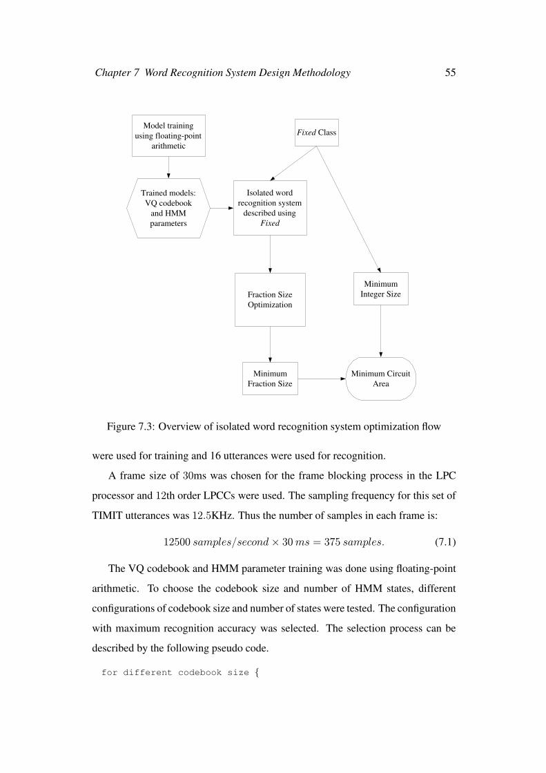
Chapter 7 Word Recognition System Design Methodology 55
Fixed Class
Isolated word recognition system
described using Fixed
Fraction Size Optimization
Minimum Circuit Area
Trained models: VQ codebook
and HMM parameters
Minimum Integer Size
Minimum Fraction Size
Model training using floating-point
arithmetic
Figure 7.3: Overview of isolated word recognition system optimization flow
were used for training and 16 utterances were used for recognition.
A frame size of 30ms was chosen for the frame blocking process in the LPC
processor and 12th order LPCCs were used. The sampling frequency for this set of
TIMIT utterances was 12.5KHz. Thus the number of samples in each frame is:
12500 samples/second× 30ms = 375 samples. (7.1)
The VQ codebook and HMM parameter training was done using floating-point
arithmetic. To choose the codebook size and number of HMM states, different
configurations of codebook size and number of states were tested. The configuration
with maximum recognition accuracy was selected. The selection process can be
described by the following pseudo code.
for different codebook size {
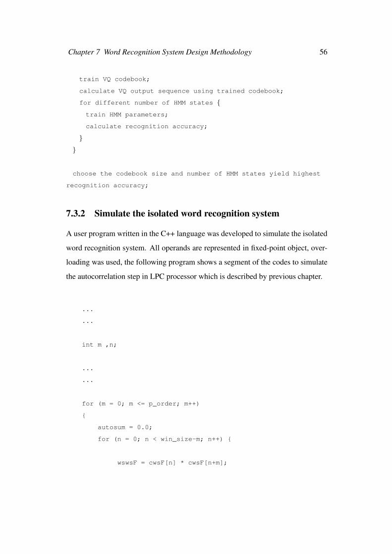
Chapter 7 Word Recognition System Design Methodology 56
train VQ codebook;
calculate VQ output sequence using trained codebook;
for different number of HMM states {train HMM parameters;
calculate recognition accuracy;
}}
choose the codebook size and number of HMM states yield highest
recognition accuracy;
7.3.2 Simulate the isolated word recognition system
A user program written in the C++ language was developed to simulate the isolated
word recognition system. All operands are represented in fixed-point object, over-
loading was used, the following program shows a segment of the codes to simulate
the autocorrelation step in LPC processor which is described by previous chapter.
...
...
int m ,n;
...
...
for (m = 0; m <= p_order; m++)
{
autosum = 0.0;
for (n = 0; n < win_size-m; n++) {
wswsF = cwsF[n] * cwsF[n+m];
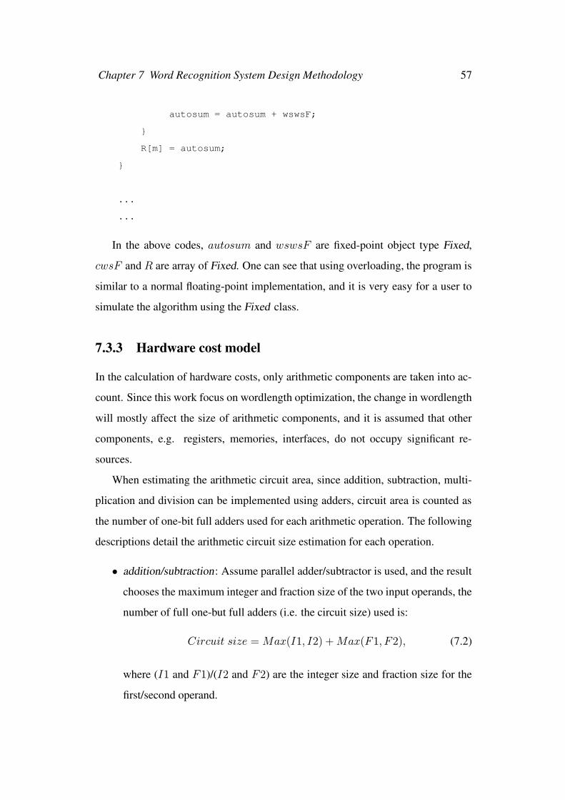
Chapter 7 Word Recognition System Design Methodology 57
autosum = autosum + wswsF;
}
R[m] = autosum;
}
...
...
In the above codes, autosum and wswsF are fixed-point object type Fixed,
cwsF and R are array of Fixed. One can see that using overloading, the program is
similar to a normal floating-point implementation, and it is very easy for a user to
simulate the algorithm using the Fixed class.
7.3.3 Hardware cost model
In the calculation of hardware costs, only arithmetic components are taken into ac-
count. Since this work focus on wordlength optimization, the change in wordlength
will mostly affect the size of arithmetic components, and it is assumed that other
components, e.g. registers, memories, interfaces, do not occupy significant re-
sources.
When estimating the arithmetic circuit area, since addition, subtraction, multi-
plication and division can be implemented using adders, circuit area is counted as
the number of one-bit full adders used for each arithmetic operation. The following
descriptions detail the arithmetic circuit size estimation for each operation.
• addition/subtraction: Assume parallel adder/subtractor is used, and the result
chooses the maximum integer and fraction size of the two input operands, the
number of full one-but full adders (i.e. the circuit size) used is:
Circuit size = Max(I1, I2) +Max(F1, F2), (7.2)
where (I1 and F1)/(I2 and F2) are the integer size and fraction size for the
first/second operand.
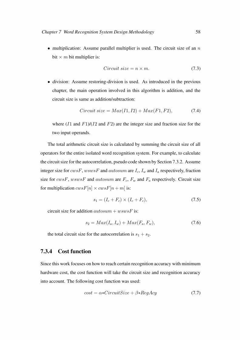
Chapter 7 Word Recognition System Design Methodology 58
• multiplication: Assume parallel multiplier is used. The circuit size of an n
bit × m bit multiplier is:
Circuit size = n×m. (7.3)
• division: Assume restoring-division is used. As introduced in the previous
chapter, the main operation involved in this algorithm is addition, and the
circuit size is same as addition/subtraction:
Circuit size = Max(I1, I2) +Max(F1, F2), (7.4)
where (I1 and F1)/(I2 and F2) are the integer size and fraction size for the
two input operands.
The total arithmetic circuit size is calculated by summing the circuit size of all
operators for the entire isolated word recognition system. For example, to calculate
the circuit size for the autocorrelation, pseudo code shown by Section 7.3.2. Assume
integer size for cwsF , wswsF and autosum are Ic, Iw and Ia respectively, fraction
size for cwsF , wswsF and autosum are Fc, Fw and Fa respectively. Circuit size
for multiplication cwsF [n]× cwsF [n+m] is:
s1 = (Ic + Fc)× (Ic + Fc), (7.5)
circuit size for addition autosum+ wswsF is:
s2 = Max(Ia, Iw) +Max(Fa, Fw), (7.6)
the total circuit size for the autocorrelation is s1 + s2.
7.3.4 Cost function
Since this work focuses on how to reach certain recognition accuracy with minimum
hardware cost, the cost function will take the circuit size and recognition accuracy
into account. The following cost function was used:
cost = α∗CircuitSize + β∗RegAcy (7.7)
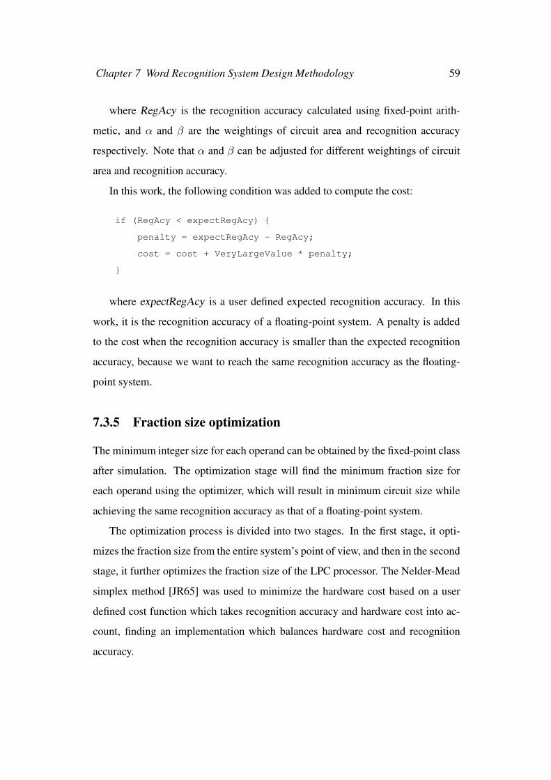
Chapter 7 Word Recognition System Design Methodology 59
where RegAcy is the recognition accuracy calculated using fixed-point arith-
metic, and α and β are the weightings of circuit area and recognition accuracy
respectively. Note that α and β can be adjusted for different weightings of circuit
area and recognition accuracy.
In this work, the following condition was added to compute the cost:
if (RegAcy < expectRegAcy) {
penalty = expectRegAcy - RegAcy;
cost = cost + VeryLargeValue * penalty;
}
where expectRegAcy is a user defined expected recognition accuracy. In this
work, it is the recognition accuracy of a floating-point system. A penalty is added
to the cost when the recognition accuracy is smaller than the expected recognition
accuracy, because we want to reach the same recognition accuracy as the floating-
point system.
7.3.5 Fraction size optimization
The minimum integer size for each operand can be obtained by the fixed-point class
after simulation. The optimization stage will find the minimum fraction size for
each operand using the optimizer, which will result in minimum circuit size while
achieving the same recognition accuracy as that of a floating-point system.
The optimization process is divided into two stages. In the first stage, it opti-
mizes the fraction size from the entire system’s point of view, and then in the second
stage, it further optimizes the fraction size of the LPC processor. The Nelder-Mead
simplex method [JR65] was used to minimize the hardware cost based on a user
defined cost function which takes recognition accuracy and hardware cost into ac-
count, finding an implementation which balances hardware cost and recognition
accuracy.
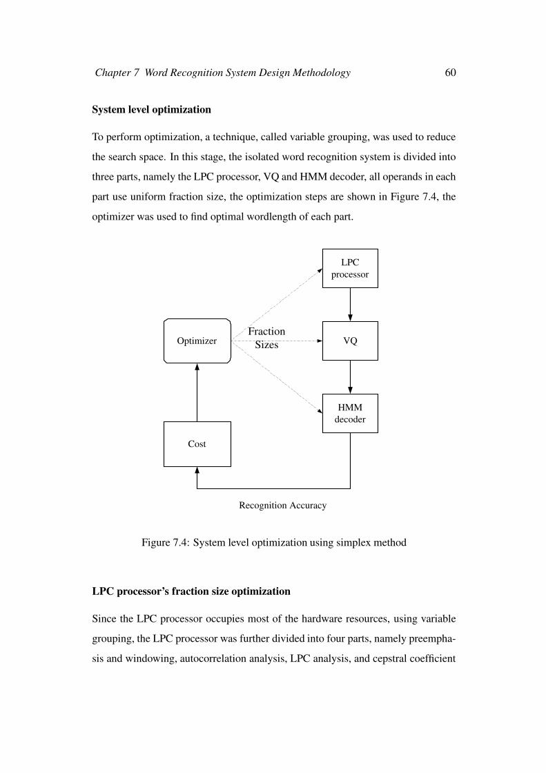
Chapter 7 Word Recognition System Design Methodology 60
System level optimization
To perform optimization, a technique, called variable grouping, was used to reduce
the search space. In this stage, the isolated word recognition system is divided into
three parts, namely the LPC processor, VQ and HMM decoder, all operands in each
part use uniform fraction size, the optimization steps are shown in Figure 7.4, the
optimizer was used to find optimal wordlength of each part.
Optimizer VQ
HMM decoder
Cost
Fraction Sizes
Recognition Accuracy
LPC processor
Figure 7.4: System level optimization using simplex method
LPC processor’s fraction size optimization
Since the LPC processor occupies most of the hardware resources, using variable
grouping, the LPC processor was further divided into four parts, namely preempha-
sis and windowing, autocorrelation analysis, LPC analysis, and cepstral coefficient
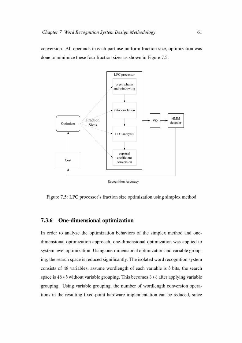
Chapter 7 Word Recognition System Design Methodology 61
conversion. All operands in each part use uniform fraction size, optimization was
done to minimize these four fraction sizes as shown in Figure 7.5.
preemphasis and windowing
LPC analysis
cepstral coefficient conversion
autocorrelation
Optimizer
LPC processor
VQ HMM
decoder
Cost
Fraction Sizes
Recognition Accuracy
Figure 7.5: LPC processor’s fraction size optimization using simplex method
7.3.6 One-dimensional optimization
In order to analyze the optimization behaviors of the simplex method and one-
dimensional optimization approach, one-dimensional optimization was applied to
system level optimization. Using one-dimensional optimization and variable group-
ing, the search space is reduced significantly. The isolated word recognition system
consists of 48 variables, assume wordlength of each variable is b bits, the search
space is 48∗ b without variable grouping. This becomes 3∗ b after applying variable
grouping. Using variable grouping, the number of wordlength conversion opera-
tions in the resulting fixed-point hardware implementation can be reduced, since
Chapter 7 Word Recognition System Design Methodology 62
the number of distinct wordlengths is reduced. The optimization steps are shown in
Figure 7.6.
Sweep fraction size of whole system
Sweep fraction size of LPC processor
Sweep fraction size of VQ
Sweep fraction size of HMM decoder
Minimum LPC processor's fraction size
implementation
Minimum VQ fraction size implementation
Minimum HMM fraction size
implementation
All operands use the same fraction
size
LPC processor, VQ and HMM use
different fraction size
Figure 7.6: System level optimization using one-dimensional optimization
1. Optimizing whole speech system’s fraction size: The whole system uses a
uniform fraction size, which is varied to find a configuration which yield min-
imum cost.
2. Optimizing the LPC processor’s fraction size: Fix the fraction size of the
VQ and HMM decoder, vary the fraction size of the LPC processor to find a
configuration which yields minimum cost.
3. Optimizing the VQ’s fraction size: Fix the fraction size of the LPC processor
and HMM decoder, vary the fraction size of the VQ to find a configuration
which yields minimum cost.
Chapter 7 Word Recognition System Design Methodology 63
4. Optimizing the HMM decoder’s fraction size: Fix the fraction size of the
LPC processor and VQ, vary the fraction size of the HMM decoder to find a
configuration which yields minimum cost.
7.4 Summary
In this chapter, the framework used to address the quantization issue of fixed-point
system was introduced. This framework was applied to an isolated word recognition
system. The detailed implementations, e.g. the speech model training, cost function
design, wordlength optimization flow, were presented.
Chapter 8
Results
8.1 Model training
One set of utterances from the TIMIT TI 46-word database [LDC] containing 20
words from 8 males and 8 females were used, there were 26 utterances for each
word, 10 were used for training and 16 were used for recognition.
The isolated word recognition system uses 12th order LPCCs, in order to choose
the VQ codebook size and number HMM state, using the method introduced in
previous chapter, different configurations of codebook size and number of state
were tested, the configuration with maximum recognition accuracy was selected.
Figure 8.1 shows the recognition accuracy for different configurations of VQ
codebook size and number of HMM states. In principle, the smaller codebook size
and number of states, the betters, since the hardware cost can be reduced. In this fig-
ure, one can see that the improvement of recognition accuracy becomes insignificant
when number of HMM states and codebook size increased. Practically, codebook
size 64 and 12 HMM states were used, this configuration doesn’t yield maximum
recognition, but this configuration can reach a certain level of recognition accuracy
with relative low cost.
64
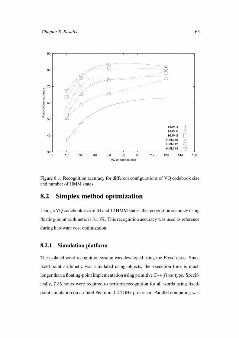
Chapter 8 Results 65
30
40
50
60
70
80
90
0 16 32 48 64 80 96 112 128 144 160
Rec
ogni
tion
accu
racy
VQ codebook size
HMM 4HMM 6HMM 8
HMM 10HMM 12HMM 14
Figure 8.1: Recognition accuracy for different configurations of VQ codebook sizeand number of HMM states
8.2 Simplex method optimization
Using a VQ codebook size of 64 and 12 HMM states, the recognition accuracy using
floating-point arithmetic is 81.3%. This recognition accuracy was used as reference
during hardware cost optimization.
8.2.1 Simulation platform
The isolated word recognition system was developed using the Fixed class. Since
fixed-point arithmetic was simulated using objects, the execution time is much
longer than a floating-point implementation using primitive C++ float type. Specif-
ically, 7.35 hours were required to perform recognition for all words using fixed-
point simulation on an Intel Pentium 4 2.2GHz processor. Parallel computing was
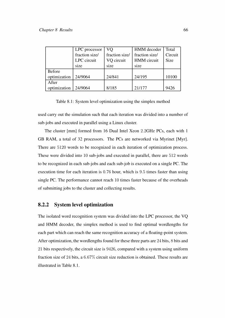
Chapter 8 Results 66
LPC processor VQ HMM decoder Totalfraction size/ fraction size/ fraction size/ CircuitLPC circuit VQ circuit HMM circuit Sizesize size size
Beforeoptimization 24/9064 24/841 24/195 10100Afteroptimization 24/9064 8/185 21/177 9426
Table 8.1: System level optimization using the simplex method
used carry out the simulation such that each iteration was divided into a number of
sub-jobs and executed in parallel using a Linux cluster.
The cluster [mm] formed from 16 Dual Intel Xeon 2.2GHz PCs, each with 1
GB RAM, a total of 32 processors. The PCs are networked via Myrinet [Myr].
There are 5120 words to be recognized in each iteration of optimization process.
These were divided into 10 sub-jobs and executed in parallel, there are 512 words
to be recognized in each sub-jobs and each sub-job is executed on a single PC. The
execution time for each iteration is 0.76 hour, which is 9.5 times faster than using
single PC. The performance cannot reach 10 times faster because of the overheads
of submitting jobs to the cluster and collecting results.
8.2.2 System level optimization
The isolated word recognition system was divided into the LPC processor, the VQ
and HMM decoder, the simplex method is used to find optimal wordlengths for
each part which can reach the same recognition accuracy of a floating-point system.
After optimization, the wordlengths found for these three parts are 24 bits, 8 bits and
21 bits respectively, the circuit size is 9426, compared with a system using uniform
fraction size of 24 bits, a 6.67% circuit size reduction is obtained. These results are
illustrated in Table 8.1.
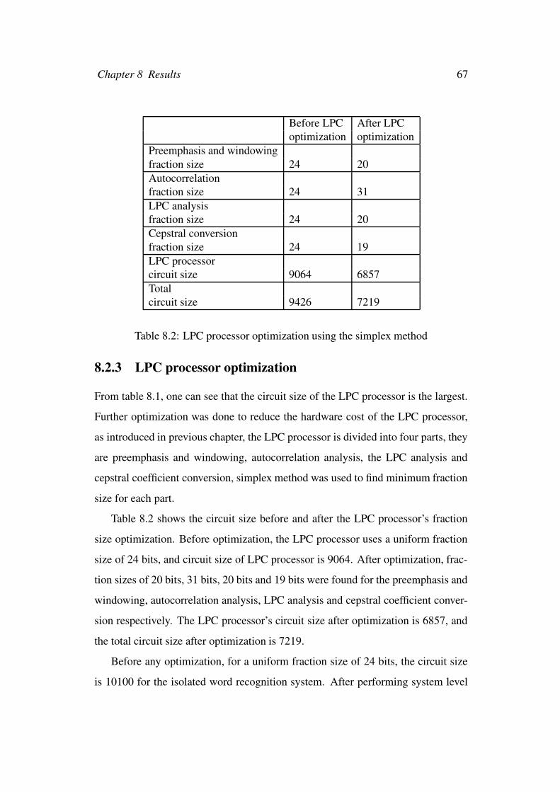
Chapter 8 Results 67
Before LPC After LPCoptimization optimization
Preemphasis and windowingfraction size 24 20Autocorrelationfraction size 24 31LPC analysisfraction size 24 20Cepstral conversionfraction size 24 19LPC processorcircuit size 9064 6857Totalcircuit size 9426 7219
Table 8.2: LPC processor optimization using the simplex method
8.2.3 LPC processor optimization
From table 8.1, one can see that the circuit size of the LPC processor is the largest.
Further optimization was done to reduce the hardware cost of the LPC processor,
as introduced in previous chapter, the LPC processor is divided into four parts, they
are preemphasis and windowing, autocorrelation analysis, the LPC analysis and
cepstral coefficient conversion, simplex method was used to find minimum fraction
size for each part.
Table 8.2 shows the circuit size before and after the LPC processor’s fraction
size optimization. Before optimization, the LPC processor uses a uniform fraction
size of 24 bits, and circuit size of LPC processor is 9064. After optimization, frac-
tion sizes of 20 bits, 31 bits, 20 bits and 19 bits were found for the preemphasis and
windowing, autocorrelation analysis, LPC analysis and cepstral coefficient conver-
sion respectively. The LPC processor’s circuit size after optimization is 6857, and
the total circuit size after optimization is 7219.
Before any optimization, for a uniform fraction size of 24 bits, the circuit size
is 10100 for the isolated word recognition system. After performing system level
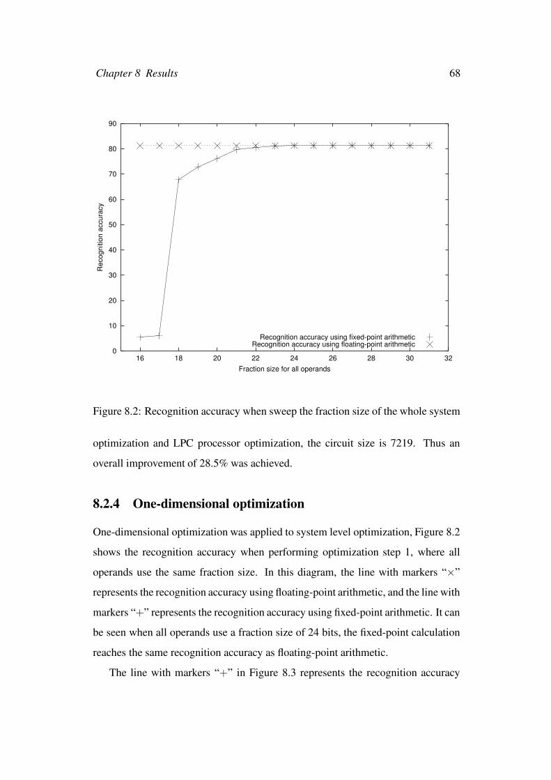
Chapter 8 Results 68
0
10
20
30
40
50
60
70
80
90
16 18 20 22 24 26 28 30 32
Rec
ogni
tion
accu
racy
Fraction size for all operands
Recognition accuracy using fixed-point arithmeticRecognition accuracy using floating-point arithmetic
Figure 8.2: Recognition accuracy when sweep the fraction size of the whole system
optimization and LPC processor optimization, the circuit size is 7219. Thus an
overall improvement of 28.5% was achieved.
8.2.4 One-dimensional optimization
One-dimensional optimization was applied to system level optimization, Figure 8.2
shows the recognition accuracy when performing optimization step 1, where all
operands use the same fraction size. In this diagram, the line with markers “×”
represents the recognition accuracy using floating-point arithmetic, and the line with
markers “+” represents the recognition accuracy using fixed-point arithmetic. It can
be seen when all operands use a fraction size of 24 bits, the fixed-point calculation
reaches the same recognition accuracy as floating-point arithmetic.
The line with markers “+” in Figure 8.3 represents the recognition accuracy
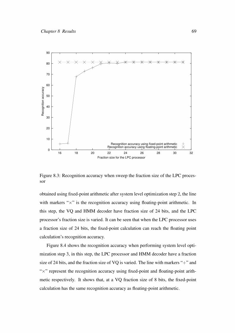
Chapter 8 Results 69
0
10
20
30
40
50
60
70
80
90
16 18 20 22 24 26 28 30 32
Rec
ogni
tion
accu
racy
Fraction size for the LPC processor
Recognition accuracy using fixed-point arithmeticRecognition accuracy using floating-point arithmetic
Figure 8.3: Recognition accuracy when sweep the fraction size of the LPC proces-sor
obtained using fixed-point arithmetic after system level optimization step 2, the line
with markers “×” is the recognition accuracy using floating-point arithmetic. In
this step, the VQ and HMM decoder have fraction size of 24 bits, and the LPC
processor’s fraction size is varied. It can be seen that when the LPC processor uses
a fraction size of 24 bits, the fixed-point calculation can reach the floating point
calculation’s recognition accuracy.
Figure 8.4 shows the recognition accuracy when performing system level opti-
mization step 3, in this step, the LPC processor and HMM decoder have a fraction
size of 24 bits, and the fraction size of VQ is varied. The line with markers “+” and
“×” represent the recognition accuracy using fixed-point and floating-point arith-
metic respectively. It shows that, at a VQ fraction size of 8 bits, the fixed-point
calculation has the same recognition accuracy as floating-point arithmetic.
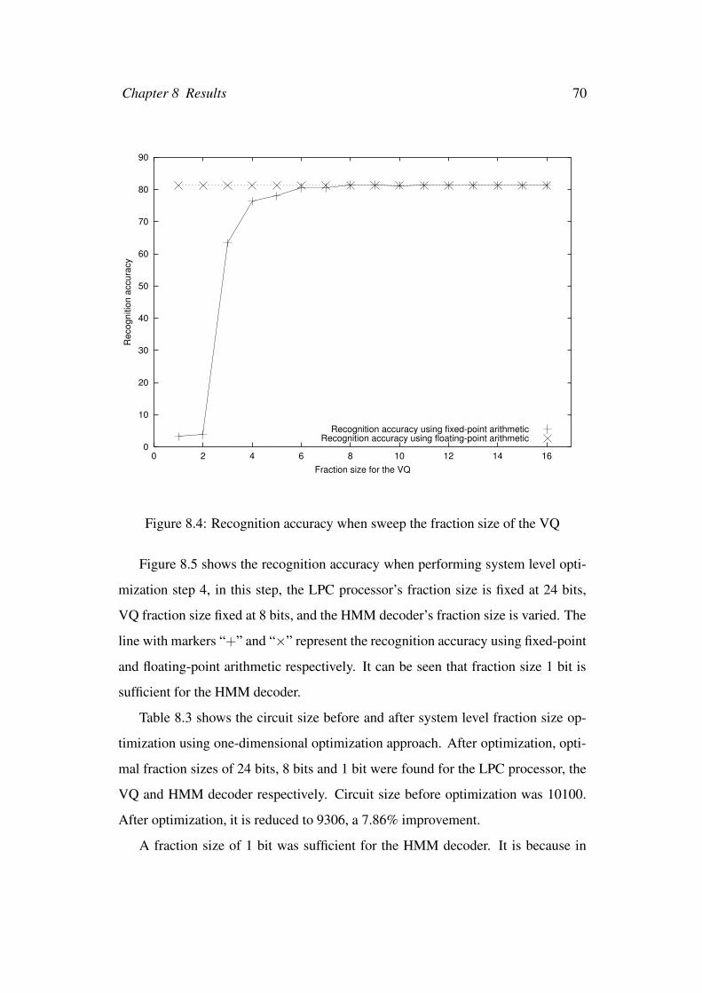
Chapter 8 Results 70
0
10
20
30
40
50
60
70
80
90
0 2 4 6 8 10 12 14 16
Rec
ogni
tion
accu
racy
Fraction size for the VQ
Recognition accuracy using fixed-point arithmeticRecognition accuracy using floating-point arithmetic
Figure 8.4: Recognition accuracy when sweep the fraction size of the VQ
Figure 8.5 shows the recognition accuracy when performing system level opti-
mization step 4, in this step, the LPC processor’s fraction size is fixed at 24 bits,
VQ fraction size fixed at 8 bits, and the HMM decoder’s fraction size is varied. The
line with markers “+” and “×” represent the recognition accuracy using fixed-point
and floating-point arithmetic respectively. It can be seen that fraction size 1 bit is
sufficient for the HMM decoder.
Table 8.3 shows the circuit size before and after system level fraction size op-
timization using one-dimensional optimization approach. After optimization, opti-
mal fraction sizes of 24 bits, 8 bits and 1 bit were found for the LPC processor, the
VQ and HMM decoder respectively. Circuit size before optimization was 10100.
After optimization, it is reduced to 9306, a 7.86% improvement.
A fraction size of 1 bit was sufficient for the HMM decoder. It is because in
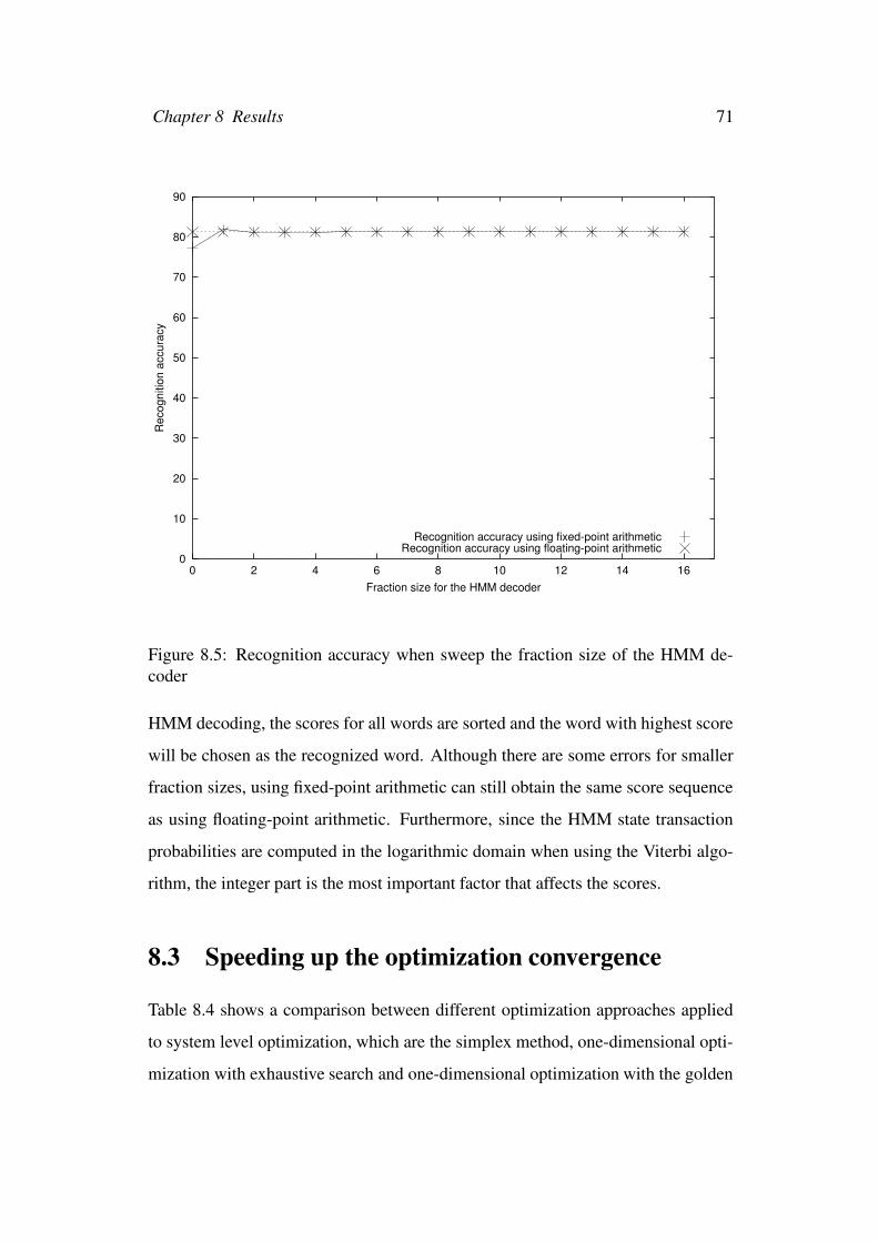
Chapter 8 Results 71
0
10
20
30
40
50
60
70
80
90
0 2 4 6 8 10 12 14 16
Rec
ogni
tion
accu
racy
Fraction size for the HMM decoder
Recognition accuracy using fixed-point arithmeticRecognition accuracy using floating-point arithmetic
Figure 8.5: Recognition accuracy when sweep the fraction size of the HMM de-coder
HMM decoding, the scores for all words are sorted and the word with highest score
will be chosen as the recognized word. Although there are some errors for smaller
fraction sizes, using fixed-point arithmetic can still obtain the same score sequence
as using floating-point arithmetic. Furthermore, since the HMM state transaction
probabilities are computed in the logarithmic domain when using the Viterbi algo-
rithm, the integer part is the most important factor that affects the scores.
8.3 Speeding up the optimization convergence
Table 8.4 shows a comparison between different optimization approaches applied
to system level optimization, which are the simplex method, one-dimensional opti-
mization with exhaustive search and one-dimensional optimization with the golden
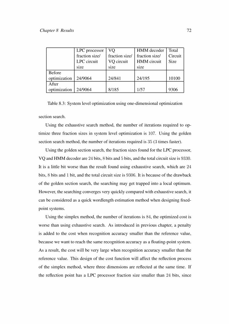
Chapter 8 Results 72
LPC processor VQ HMM decoder Totalfraction size/ fraction size/ fraction size/ CircuitLPC circuit VQ circuit HMM circuit Sizesize size size
Beforeoptimization 24/9064 24/841 24/195 10100Afteroptimization 24/9064 8/185 1/57 9306
Table 8.3: System level optimization using one-dimensional optimization
section search.
Using the exhaustive search method, the number of iterations required to op-
timize three fraction sizes in system level optimization is 107. Using the golden
section search method, the number of iterations required is 35 (3 times faster).
Using the golden section search, the fraction sizes found for the LPC processor,
VQ and HMM decoder are 24 bits, 8 bits and 5 bits, and the total circuit size is 9330.
It is a little bit worse than the result found using exhaustive search, which are 24
bits, 8 bits and 1 bit, and the total circuit size is 9306. It is because of the drawback
of the golden section search, the searching may get trapped into a local optimum.
However, the searching converges very quickly compared with exhaustive search, it
can be considered as a quick wordlength estimation method when designing fixed-
point systems.
Using the simplex method, the number of iterations is 84, the optimized cost is
worse than using exhaustive search. As introduced in previous chapter, a penalty
is added to the cost when recognition accuracy smaller than the reference value,
because we want to reach the same recognition accuracy as a floating-point system.
As a result, the cost will be very large when recognition accuracy smaller than the
reference value. This design of the cost function will affect the reflection process
of the simplex method, where three dimensions are reflected at the same time. If
the reflection point has a LPC processor fraction size smaller than 24 bits, since
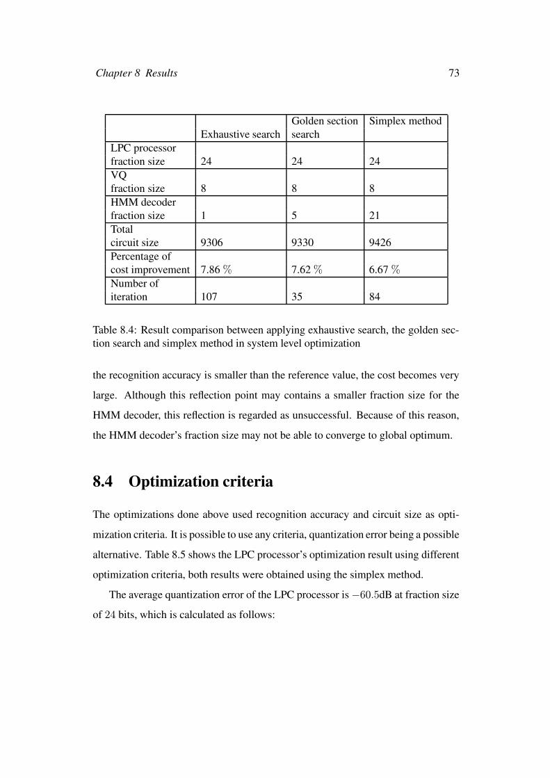
Chapter 8 Results 73
Golden section Simplex methodExhaustive search search
LPC processorfraction size 24 24 24VQfraction size 8 8 8HMM decoderfraction size 1 5 21Totalcircuit size 9306 9330 9426Percentage ofcost improvement 7.86 % 7.62 % 6.67 %Number ofiteration 107 35 84
Table 8.4: Result comparison between applying exhaustive search, the golden sec-tion search and simplex method in system level optimization
the recognition accuracy is smaller than the reference value, the cost becomes very
large. Although this reflection point may contains a smaller fraction size for the
HMM decoder, this reflection is regarded as unsuccessful. Because of this reason,
the HMM decoder’s fraction size may not be able to converge to global optimum.
8.4 Optimization criteria
The optimizations done above used recognition accuracy and circuit size as opti-
mization criteria. It is possible to use any criteria, quantization error being a possible
alternative. Table 8.5 shows the LPC processor’s optimization result using different
optimization criteria, both results were obtained using the simplex method.
The average quantization error of the LPC processor is−60.5dB at fraction size
of 24 bits, which is calculated as follows:
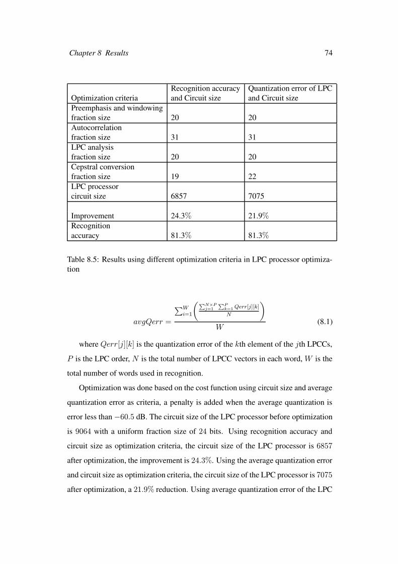
Chapter 8 Results 74
Recognition accuracy Quantization error of LPCOptimization criteria and Circuit size and Circuit sizePreemphasis and windowingfraction size 20 20Autocorrelationfraction size 31 31LPC analysisfraction size 20 20Cepstral conversionfraction size 19 22LPC processorcircuit size 6857 7075
Improvement 24.3% 21.9%Recognitionaccuracy 81.3% 81.3%
Table 8.5: Results using different optimization criteria in LPC processor optimiza-tion
avgQerr =
∑Wi=1
(∑N×Pj=1
∑Pk=1 Qerr[j][k]
N
)
W(8.1)
where Qerr[j][k] is the quantization error of the kth element of the jth LPCCs,
P is the LPC order, N is the total number of LPCC vectors in each word, W is the
total number of words used in recognition.
Optimization was done based on the cost function using circuit size and average
quantization error as criteria, a penalty is added when the average quantization is
error less than−60.5 dB. The circuit size of the LPC processor before optimization
is 9064 with a uniform fraction size of 24 bits. Using recognition accuracy and
circuit size as optimization criteria, the circuit size of the LPC processor is 6857
after optimization, the improvement is 24.3%. Using the average quantization error
and circuit size as optimization criteria, the circuit size of the LPC processor is 7075
after optimization, a 21.9% reduction. Using average quantization error of the LPC
Chapter 8 Results 75
processor and circuit size as criteria, the result is similar to that using recognition
accuracy and circuit size as criteria.
8.5 Summary
This chapter presented the results for the optimization of an isolated word recogni-
tion system. An overall circuit size reduction of 28.5% was achieved. The golden
section search method can be used to speed up the searching and was shown to be
3 times faster than an exhaustive search. The results using different optimization
criteria were also analyzed. Using average quantization error of the LPC processor
as criteria, a 21.9% circuit size reduction of the LPC processor was obtained, while
a 24.3% reduction was achieved using recognition accuracy as criteria.
Chapter 9
Conclusion
A framework was introduced to address the quantization issues of fixed-point sys-
tem, an isolated word recognition system was used to explore the utility of the
framework. The isolated word recognition system uses 12th order LPCCs, code-
book size 64 and 12 HMM states, the recognition accuracy is 81.3% using floating-
point arithmetic, this recognition accuracy was used as reference during hardware
cost optimization. An application program was developed to simulate the speech
system using the fixed-point class, when all operands use a uniform fraction size
of 24 bits, the circuit size is 10100. After performing hardware cost optimization
using the optimizer, the circuit size is 7219, a 28.5% reduction was obtained. The
problems addressed are stated below:
9.1 Search space reduction
One-dimensional optimization and variable grouping were used to reduce the search
space. The isolated word recognition system contains 48 variables, each variable
has fraction size 32 bits, the search space is 4833, after applying the one-dimensional
optimization, the search space becomes 48 × 33. Using variable grouping, the
speech system was divided into three components, the LPC processor, the VQ
and HMM decoder, each part uses uniform fraction size, the search space becomes
76
Chapter 9 Conclusion 77
3 × 33. Variable grouping was used to further optimize the cost of the LPC pro-
cessor, where the LPC processor is divided into the preemphasis and windowing,
the autocorrelation, the LPC analysis and the cepstral coefficient conversion. After
applying the one-dimensional optimization to optimize the speech system in system
level optimization, a 7.86% circuit size reduction was obtained, which is a little bit
better than the simplex method, where a 6.67% reduction was achieved.
9.2 Speeding up the searching
The golden section search method was used to speed up searching. Using this ap-
proach, the searching can be 3 times faster than exhaustive search and achieve sim-
ilar results. In the system level optimization, the difference between the final costs
was only 0.24%. Using exhaustive search, the fraction sizes of the LPC processor,
VQ and HMM decoder were 24 bits, 8 bits and 1 bit respectively, however, fraction
sizes of 24 bits, 8 bits and 5 bits were obtained using the golden section search.
Since the searching converges very quickly using the golden section search, the
one-dimensional optimization with the golden section search can be considered as
a quick wordlength estimation method.
9.3 Optimization criteria
The cost function used in this work was based primarily on recognition accuracy,
since this is a direct measure of the system’s performance. However, as described
in Section 8.4, other optimization criteria such as quantization error could be used,
and in fact may be more suitable for other applications with real valued outputs such
as filtering etc.
Chapter 9 Conclusion 78
When optimizing the cost of the LPC processor, the results obtained using dif-
ferent optimization criteria were compared. Using recognition accuracy as a crite-
ria, a cost of 6857 was obtained for the LPC processor, which is a 24.3% improve-
ment, while a cost of 7075 was obtained using average quantization error of the
LPCCs as criteria, the improvement is 21.9%, the simplex method was applied to
do the experiments, the difference of the optimized cost is 2.4%.
9.4 Flexibility of the framework design
Using object oriented concept, each part of the framework can be developed inde-
pendently, modification to one part will not affect the design of other parts. Using
overloading, the fixed-point simulation description can be developed easily. Since
optimization was done based on a cost function, by modifying the attributes of the
cost function, different optimization results can be analyzed easily.
The fixed-point class can automatically trace the range information of each vari-
able and determine the integer size, moreover, it can perform calculations using both
floating-point and fixed-point arithmetic simultaneously and calculate the quantiza-
tion error automatically. Quantization effect of the fixed-point system can be ana-
lyzed conveniently.
9.5 Further development
Currently, the cost model only considers the hardware cost of arithmetic compo-
nents, other components, e.g. memories, interfaces, were assumed occupying in-
significant resources. A more accurate model can be developed, which will take
these factors into account. Moreover, timing constraint can also be considered, e.g.
logic delay, clock cycles can be added into the cost.
A more robust error reporting mechanism can be used. For example, each object
can be associated with a flag, which can indicate arithmetic error, such as overflow

Chapter 9 Conclusion 79
and underflow, occurred during simulation.
Bibliography
[Amo94] Amos R. Omondi. Computer Arithmetic Systems: Algorithms, Archi-
tecture and Implementation. Prentice Hall, 1994.
[BM91] B. Nowrouzian and M.J. Svihura. High speed real-time design and
implementation of Cauer-type Jaumann digital filters. In Proceedings
of the 34th Midwest Symposium on Circuits and Systems, pages 692–
695, 1991.
[CZS02] Carl Hamacher, Zvonko Vranesic, and Safwat Zaky. Computer Orga-
nization, fifth edition. McGraw-Hill Companies, Inc, 2002.
[FBM98] Fengying Yao, Bizhou Li, and Min Zhang. A fixed-point DSP im-
plementation for a low bit rate vocoder. In Proceedings of the 5th
International Conference on Solid-State and Integrated Circuit Tech-
nology, pages 365–368, 1998.
[FRD01] Fabian Luis Vargas, Rubem Dutra Ribeiro Fagundes, and Daniel Bar-
ros Junior. A FPGA-Based Viterbi Algorithm Implementation for
Speech Recognition Systems. In IEEE International Conference on
Acoustics, Speech, and Signal Processing, pages 1217–1220, Vol.2,
2001.
[GKZ98] Guanghui Hui, Kwok-Chiang Ho, and Zenton Goh. A robust speaker-
independent speech recognizer on ADSP2181 fixed-point DSP. In
80
1998 Fourth International Conference on Signal Processing, pages
694–697 vol.1, 1998.
[HMMH98] H. Keding, M. Willems, M. Coors, and H. Meyr. FRIDGE: A Fixed-
Point Design And Simulation Environment. In Design, Automation
and Test in Europe (DATE-98), 1998.
[IK99] Iman Gholampour and Kambiz Nayebi. High performance telephony
speech recognition via cascade HMM/ANN hybrid. In International
Symposium on Signal Processing and Its Applications, pages 645–648
vol.2, 1999.
[Isr02] Israel Koren. Computer Arithmetic Algorithms. Prentice Hall, 2002.
[JD99] John L. Hennessy and David A. Patterson. Computer Architecture: A
Quantitative Approach 2nd Edition. Morgan Kaufmann, 1999.
[JR65] J. Nelder and R. Mead. A simplex method for function minimization.
In Computer Journal, Vol. 7, pages 308–313, 1965.
[Kai79] Kai Hwang. Computer Arithmetic: Principles, Architecture, and De-
sign. John Wiley & Sons, Inc, 1979.
[KGR97] Kun-Shan Lin, Gene A. Frantz, and Ray Simar, Jr. The TMS320 Fam-
ily of Digital Signal Processors. Texas Instruments, 1997.
[KJK95] K.K. Shin, J.C.H. Poon, and K.C. Li. A fixed-point DSP based Can-
tonese recognition system. In IEEE International Symposium on In-
dustrial Electronics, pages 390–393 vol.1, 1995.
[KJW00] Ki-II Kum, Jiyang Kang, and Wonyong Sung. AUTOSCALER for C:
an optimizing floating-point to integer C program converter for fixed-
point digital signal processors. In IEEE Transactions on Circuits and
81
Systems II: Analog and Digital Signal Processing, Vol. 47, Issue: 9,
pages 840–848, 2000.
[LB93] Lawrence Rabiner and Biing-Hwang Juang. Fundamentals of Speech
Recognition. Prentice Hall PTR, 1993.
[LDC] LDC. http://www.ldc.upenn.edu.
[mm] Department of Computer science and Engineering, the Chinese University of
Hong Kong. http://www.cse.cuhk.edu.hk/corner/tech/doc/system/hpc/myrinet/.
[MM98] M. Jersak and M. Willems. Fixed-Point Extended C Compiler Al-
lows More Efficient High-Level Programming of Fixed-Point DSPs.
In 9th International Conference on Signal Processing Applications &
Technology (ICSPAT’98), 1998.
[MS02] Mark L. Chang and Scott Hauck. Precis: A Design-Time Precision
Analysis Tool. In IEEE Symposium on Field-Programmable Custom
Computing Machines, pages 229–238, 2002.
[Myr] Myricom, Inc. http://www.myri.com/.
[NNS+99] Nishida, Y., Nakadai, Y., Suzuki, Y., Sakurai, T., Kurokawa, T., and
Sato, H. Voice recognition focusing on vowel strings on a fixed-point
20-MIPS DSP board. In IEEE International Conference on Acoustics,
Speech, and Signal Processing, pages 137–140 vol.1, 1999.
[P. 91] P. W. Wong. Quantization and Roundoff Noises in Fixed-Point FIR
Digital Filters. In IEEE Transactions on Signal Processing, Vol. 39,
No 7, 1991.
[Pau98] Paul D. Fiore. Lazy Rounding. In 1998 IEEE Workshop on Signal
Processing Systems (SiPS’98), 1998.
82
[RJ87] R. A. Pepe and J. D. Rogers. Simulation of Fixed-Point Operations
with High-Level Languages. In IEEE Transactions on Acoustics,
Speech, and Signal Processing, Vol. 35, No 1,, 1987.
[RLP+99] R. Cmar, L. Rijnders, P. Schaumont, S. Vernalde, and I. Bolsens. A
Methodology and Design Environment for DSP ASIC Fixed Point Re-
finement. In Proceedings of the Design Automation and Test in Europe
conference, pages 271–276, 1999.
[SA98] Suhrid A. Wadekar and Alice C. Parker. Accuracy Sensitive Word-
Length Selection for Algorithm Optimization. In International Con-
ference on Computer Design - ICCAD, 1998.
[Sin96] Singiresu S. Rao. Engineering optimization, theory and practice, third
edition. John Wiley & Sons, Inc., Wiley Eastern Limited, Publishers,
and New Age International Publishers, Ltd, 1996.
[SIYS96] Sung-Nam Kim, In-Chui Hwang, Young-Woo Kim, and Soo-Won
Kim. A VLSI chip for isolated speech recognition system. In IEEE
Transactions on Consumer Electronics, Volume: 42, Issue: 3, pages
458–467, 1996.
[SKW95] S. Kim, K. Kum, and W. Sung. Fixed-Point Optimization Utility for
C and C++ Based Digital Signal Processing Programs. In Workshop
on VLSI and Signal Processing, Osaka, November 1995.
[SSM02] S.J. Melnikoff, S.F. Quigley, and M. J. Russell. Implementing a Sim-
ple Continuous Speech Recognition System on an FPGA. In Field-
Programmable Custom Computing Machines, pages 275–276, 2002.
[SW98] Seehyun Kim and Wonyong Sung. Fixed-Point Error Analysis and
Word Length Optimization of 8×8 IDCT Architectures. In IEEE
83
Transactions on Circuits and Systems for Video Technology Volume
8 Number 8, pages 935–940, December 1998.
[Voj02] Vojin G. Oklobdzija. The Computer Engineering Handbook. CRC
Press LLC, 2002.
[Wil00] William Stallings. Computer organization and architecture, fifth edi-
tion. Prentice-Hall, Inc, 2000.
[WK95] Wonyong Sung and Ki-II Kum. Simulation-Based Word-Length Opti-
mization Method for Fixed-Point Digital Signal. In IEEE Transactions
on Signal Processing, Vol. 43, No 12, December 1995.
[WL89] William G. Bliss and Louis L. Scharf. Algorithms and Architectures
for Dynamic Programming on Markov Chains. In IEEE Transactions
on Acoustics, Speech and Signal Processing, pages 900–912, Vol.37,
Issue: 6, 1989.
[WM94] William Cammack and Mark Paley. Fixpt: A C++ Method for De-
velopment of Fixed Point Digital Signal Processing Algorithms. In
Proceeding of the Twenty-Seventh Hawaii International Conference
on System Science, Vol. I: Architecture, 1994.
[WSWB92] William H. Press, Saul A. Teukolsky, William T. Vetterling, and Brian
P. Flannery. Numerical Recipes in C: The Art of Scientific Computing
Second Edition. Cambridge University Press, 1992.
[YCR+94] Y. Zhang, C.J.S. deSilva, R. Togneri, M. Alder, and Y. Attikiouzel.
Speaker-independent isolated word recognition using multiple hidden
Markov models. In IEEE Proceedings of Vision, Image and Signal
Processing, Volume: 141, Issue: 3, pages 197–202, 1994.
[YY00] Yifan Gong and Yu-Hung Kao. Implementing a high accuracy
speaker-independent continuous speech recognizer on a fixed-point
84

DSP. In IEEE International Conference on Acoustics, Speech, and
Signal Processing, pages 3686–3689 vol.6, 2000.
85
Publications
Full Length Conference Papers
• Y.M. Lam, M.W. Mak and P.H.W. Leong: Fixed-Point Implementations of
Speech Recognition Systems, Proceedings of the International Signal Pro-
cessing Conference, DALLAS 2003
86