An Optimal Hierarchical Clustering Approach to Mobile

This article has been accepted for inclusion in a future issue of this journal. Content is final as presented, with the exception of pagination.

IEEE TRANSACTIONS ON INTELLIGENT TRANSPORTATION SYSTEMS 1

An Optimal Hierarchical Clustering Approach toMobile LiDAR Point Clouds

Sheng Xu , Ruisheng Wang , Hao Wang, and Han Zheng

Abstract— This paper aims to propose a new optimal hier-archical clustering approach to 3D mobile light detection andranging (LiDAR) point clouds. The hierarchical clustering isperformed on unorganized point clouds based on a proximitymatrix that consists of a distance term and a direction term.In the dissimilarity calculation of two clusters, a pair of pointsfrom each of two clusters is selected, respectively, and Euclideandistances between the points are employed to define the distanceterm. The direction term is obtained by the differences of normalvectors at chosen points. The main contribution is that the clustercombination in the hierarchical clustering is optimized by apoint-based graph model. The cluster combination is formulatedas a problem of matching, optimized by finding the minimum-costperfect matching in a bipartite graph. The results show thatthe proposed hierarchical clustering method succeeds in seg-menting object from point clouds without any human–computerinteraction and outperforms the state-of-the-art segmentationapproaches in terms of completeness and correctness.

Index Terms— Hierarchical clustering, MLS, segmentation,bipartite graph.

I. INTRODUCTION

SEGMENTATION from point clouds collected by lasersensors plays an important role in the environmental

analysis, 3D modeling and object tracking. Segmentation is theprocess of partitioning input data into multiple regions. Seg-mentation results can be divided into three levels, namely thesupervoxel level [1], region level [2] and object level [3], [4].Nowadays, segmentation results have been effectively usedin applications related to the navigation of a self-driving car,such as the curb extraction [5], pedestrian detection [6], streetlight poles localization [7] and simultaneous localization andmapping (SLAM) [8]. The key challenge in segmentation ofpoint clouds is the split of overlapping regions. Due to the factthat point clouds are noisy, uneven and unorganized i.e. lackof topology, overlapping regions are difficult to be detected.

This paper aims to propose a new optimal hierarchicalclustering (OHC) approach to mobile LiDAR (Light Detection

Manuscript received September 11, 2018; revised January 21, 2019;accepted March 31, 2019. The Associate Editor for this paper was J. Li.(Corresponding author: Ruisheng Wang.)

S. Xu is with the College of Information Science and Technology, NanjingForestry University, Nanjing 210037, China.

R. Wang is with the School of Geographical Sciences, Guangzhou Univer-sity, Guangzhou 510006, China, and also with the Department of GeomaticsEngineering, University of Calgary, Calgary, AB T2N 1N4, Canada (e-mail:[email protected]).

H. Wang is with the College of Landscape Architecture, Nanjing ForestryUniversity, Nanjing 210037, China.

H. Zheng is with the Department of Geomatics Engineering, University ofCalgary, Calgary, AB T2N 1N4, Canada.

Digital Object Identifier 10.1109/TITS.2019.2912455

And Ranging) point clouds. The approach uses the matchingin a bipartite graph to combine regions, and the optimal clustercombination is solved by the minimum-cost perfect matchingin the point-based graph. In this paper, a region is regardedas a component of an object instance. Points from one regionshould not belong to different object instances. For example,one building instance may include one or several regions.

This paper is organized as follows. Section II reviews meritsand demerits of the related segmentation methods. Section IIIdescribes the overall idea of the optimal hierarchical cluster-ing (OHC) algorithm. Section IV focuses on the determinationof the dissimilarity between clusters to form the proximitymatrix. Section V uses the matching in a bipartite graphto find the combination solution and achieves the optimalcombination by solving the minimum-cost perfect matching.Section VI shows experiments to evaluate the performanceof the proposed method. Section VII demonstrates mergingresults of regions and discusses complexity of the proposedOHC. Conclusions are outlined in Section VIII.

II. RELATED WORK

In this paper, the segmentation is related to the split ofgeneral instances from an input scene, which is different fromthe specific instance extraction or detection. In the objectextraction, commonly used methods are rule-based. In thework of Zhang et al. [5], they segment road curbs based onpredefined rules, including the planar surface of roads andthe elevation difference between curbs and roads. In the workof Li et al. [6], the detection of pedestrian is based on thedensity requirement and geometric shape. In the work ofWu et al. [7], the extraction of poles is based on the featureextraction, including pole features and geometric information.Those methods are difficultly used in the segmentation ofgeneral object instances. Related work for the multi-objectsegmentation is shown below.

In the work of Douillard et al. [9], the authors proposea Cluster-All method for dense point clouds and achievea trade-off in terms of simplicity, accuracy and computa-tion time. The grouping process in Cluster-All is based onthe k-nearest neighbors approach. The principle of KNNiPC(k-nearest neighbors in point clouds) is selecting a numberof points for a given point based on the nearest Euclid-ean distance and assigning them the same index. To avoidunder-segmentation results, the variance and mean of Euclid-ean distances of the points within a group are restricted to beless than a preset threshold. A similar approach is shown in

1524-9050 © 2019 IEEE. Personal use is permitted, but republication/redistribution requires IEEE permission.See http://www.ieee.org/publications_standards/publications/rights/index.html for more information.

https://orcid.org/0000-0002-9017-1510

https://orcid.org/0000-0003-0745-5158


2 IEEE TRANSACTIONS ON INTELLIGENT TRANSPORTATION SYSTEMS

the work of Klasing et al. [10]. The authors present a radiallynearest neighbors strategy to bound the region of neighborpoints, which helps enhance the robustness of the neighborselection. The KNNiPC works well in different terrain areasand does not require any prior knowledge of object locations.The problem is that results of KNNiPC highly depend onthe selection of a “good value” for k which is the numberof selected nearest neighbor points. The setting of k is verysensitive to the point cloud density. A large k fails to splitoverlapping regions between different object instances and asmall one may cause a heavy over-segmentation.

In the point cloud segmentation, the challenging is to sep-arate two overlapping regions. In the method of Yu et al. [3],the authors propose an algorithm for segmenting pole-likeobjects from mobile LiDAR point clouds. In order to separate acluster with more than one object, the authors add the elevationinformation to extend the 2D normalized-cut method [11].The 3DNCut (3D normalized-cut) partitions input points intotwo disjoint groups by minimizing the dissimilarity withineach group and maximizing the dissimilarity between differentgroups. 3DNCut obtains an optimal solution of the binary seg-mentation, which demonstrates a promising method for mobileLiDAR point cloud segmentation. The shortcoming is that thenumber of regions has to be preset before the segmentation.In the method of Golovinskiy et al. [4], the authors presenta min-cut based method (MinCut) for segmenting objectsfrom point clouds. The MinCut partitions input points intotwo disjoint groups, i.e. background and foreground, by min-imizing Euclidean distances between graph points and thesource/sink node. The solution cut, which is used to separatethe input scene into background and foreground, is obtained bythe graph cut method [12]. The MinCut obtains competitivesegmentation results in terms of the optimum and accuracy.However, users have to set the center point and radius foreach object. Recently, Su et al. [13] propose a segmentationmethod for terrestrial LiDAR scans of industrial sites con-taining piping systems. Their split and merge procedures firstseparate voxel points into spatially unconnected components,and then intelligently merge these components using a seriesof connectivity criteria across voxels. However, the space com-plexity is high and the merging procedure depends on a seriesof connectivity criteria (proximity, orientation, and curvature),which is difficult calculated in a general traffic scene. In thework of Lin et al. [14], they formalize segmentation as a subsetselection problem and develop an heuristic algorithm to solvethe selection problem. Their extracted supervoxels preserve theobject boundaries and structures with a higher boundary recalland lower under-segmentation error. The problem is that thesupervoxel formulation in vegetation is difficult because theboundary of vegetation is blurred.

Clustering is a well-known technique in data mining. Thecommonly used is the k-means approach, which has been usedfor the point cloud in [15], [16]. The idea of KMiPC (k-meansin point clouds) is to partition points into different sets tominimize the sum of distances of each point in the cluster tothe center. In the work of Lavoué et al. [15], the authors usek-means for the extraction of ROI (region of interest) frommesh points. The problem is that KMiPC is easy to produce

excessive segments as indicated in [15]. Moreover, the KMiPCneeds to set the number of clusters and fails to segmentoverlapping regions [16]. In the work of Feng et al. [17],the authors propose a planar region extraction method basedon the agglomerative clustering approach (PEAC) and suc-ceed in segmenting regions from point clouds efficiently. Theshortcoming is that input point clouds are required to be well-organized.

The accuracy of KMiPC and KNNiPC is sensitive to pointcloud density and is decreased in the overlapping regionsbetween different object instances. The accuracy of 3DNcutand MinCut depends on the scene and can be low when thenumber of objects is large. The accuracy of PEAC relies onthe geometric information and is reduced when objects havecomplex shapes. In this paper, we propose a new hierarchicalclustering algorithm for LiDAR point clouds. The clustercombination is optimized by solving the minimum-cost perfectmatching in a bipartite graph. The proposed algorithm does notrequire the initial number of clusters or the location of objects,which is significant in the point cloud clustering.

III. THE OVERALL IDEA OF THE OPTIMAL HIERARCHICAL

CLUSTERING (OHC)

In this paper, the proposed OHC is based on a bottom-upstrategy to group regions. It starts with a cluster set, andeach set consists of only one point. Then, it measures thedissimilarity between clusters and combines similar clustersinto a new cluster.

The input point set is P = {p1, p2, . . . , pn}, and the resul-tant cluster set is C = {c1, c2, ...ci , . . . , c j , . . . , ct }, where nis the number of points in P and t is the number of clustersin C . Each cluster ci contains one or more points from P ,and ci ∩ c j is Ø under i �= j . The proximity matrix is PM,which is used to measure the dissimilarity between clustersin C . The goal of the proposed OHC is to optimize the setC , so that each ci ∈ C is a cluster of a region. The objectivefunction for the minimization is

arg min�

∑

{ca,cb}∈�

PM(ca, cb), (1)

where � is the set of the neighboring clusters to be com-bined. The matrix element PM(ca, cb) means the dissimilaritybetween the cluster ca and cb.

In the initialization, each cluster ci contains only one pointfrom P , and the size of the proximity matrix is t × t . In theproposed OHC, similar clusters are combined into one clusterand the value of t will be reduced during the clusteringprocess. Key steps are the determination of the proximitymatrix and the optimization of the cluster combination, whichwill be discussed in the following sections. The correspondingflowchart is shown in Fig.1. The cluster set Ci+1 is the updateof Ci based on the optimal cluster combination. At the end ofthe algorithm, the converged cluster set C is regarded as theclustering result.

IV. DETERMINATION OF THE PROXIMITY MATRIX

For a set C with t clusters, we formulate a t × t symmetricproximity matrix. The (i, j)th element of the matrix means


XU et al.: OHC APPROACH TO MOBILE LiDAR POINT CLOUDS 3

Fig. 1. The flowchart of the proposed OHC approach.

the dissimilarity between the i th and j th cluster (i, j =1, 2, . . . , t). During the hierarchical clustering, two clusterswith a low dissimilarity are preferred to be combined intoone cluster. In this paper, points from a region are assumedto be spatially close, and normal vectors at points from localplanes are similar. The calculation of the dissimilarity containsa distance measure α

(pi , p j , ci , c j

)and a direction measure

β(

pi , p j , ci , c j).

The density of LiDAR points relies on the scanning patternand the distance to the sensor, therefore, Euclidean distancesbetween points are various in different regions. In order toimprove the robustness of the distance calculation, we normal-ize Euclidean distances between points. The normalization isachieved by using a scalar value. Commonly used filters forthis purpose are the maximum, minimum and median filters.The maximum filter is sensitive to clusters with outliers. Theminimum filter achieves 0 when there exist duplicate points ina region. In the calculation of α


), the required

scalar values f (ci ) and f (c j ) are based on the median filterMed , which is defined as Eq.(2).

f (ci ) = Medp∈ci { minp′∈ci ,p′ �=p

d(p, p′)} (2)

For example, if one has a cluster c0 = {p1, p2, p3} andthe minimal distance from each point pi ∈ c0 to otherpoints within c0 is di , f (c0) is obtained by the median valueof {d1, d2, d3}. It is worth noting that if there is only onepoint in the cluster ci , f (ci ) will be 1. The distance termα


)is formed as

α(

pi , p j , ci , c j) = d(pi , p j )

max( f (ci ), f (c j ))(3)

where d(pi , p j ) measures Euclidean distances between twopoints. Clusters ci and c j are two different clusters in theset C . Points pi and p j are obtained by

arg min(pi ,p j )

d(pi , p j ) : pi ∈ ci , p j ∈ c j (4)

The direction measure is based on the normal vector infor-mation. The normal vector at a point is approximated as thenormal to the surface estimated by its k-nearest neighborhoodpoints. Assuming that there are k points in the estimation,based on singular value decomposition (SVD) method one has

⎡

⎢⎢⎣

x1 y1 z1x2 y2 z2. . . . . . . . .xk yk zk

⎤

⎥⎥⎦ = Dk×3 = Uk×kSk×3V�3×3 (5)

where D is the input matrix decomposed into the matricesU, S and V. The column vector V| in V, which correspondsto the smallest eigenvalue in the decomposition, is chosenas the normal vector at the given point. The direction termβ


)is formed as

β(

pi , p j , ci , c j) = 1 −

∣∣∣V|(pi) · V|(p j )∣∣∣ (6)

where V|(pi ) and V|(p j ) are normal vectors estimated fromthe k-nearest neighbors of the point pi and p j , respectively.Points pi and p j are obtained by Eq.(4).

In our work, exterior points are defined as the outer surfacepoints of object instances, and interior points are the restof points. If two objects are connected with each other,objects’ exterior points are potential to be the overlappingpoints between different objects. The proximity matrix PMis calculated by Eq.(7), shown at the bottom of the next page.λ is a user-defined coefficient to balance α


)and

β(

pi , p j , ci , c j). If both pi and p j are interior points, which

are assumed to be in the same cluster, the calculation of PMis based on Eq.(7a); if both of them are exterior points, whichcan be in different clusters, the calculation of PM is basedon Eq.(7b); in all other conditions, the calculation of PM isbased on Eq.(7c). The dissimilarity between two clusters issmall if they are spatially close or they have consistent normalvectors at the given points obtained by Eq.(4). When bothtwo clusters consist of interior points, the dissimilarity will bedominated by the distance measure. When both two clustersconsist of exterior points, the direction measure dominatestheir dissimilarity.

In the work of Chaudhuri and Chaudhuri [18], the authorsdevelop a detection approach to distinguish border pointsin a dot pattern. The assumption is that border points arenot surrounded by other points in all directions and theauthors detect border points efficiently in synthetic pointclouds. However, mobile LiDAR point clouds are complex,uneven and incomplete. The threshold to determine borderpoints is required to be adaptive for different regions. Anothercommonly used method for the shape calculation is called 3Dα-shape [19]. It succeeds in recovering the shape ofnon-convex and even non-connected sets in 3D point clouds.However, since MLS point clouds are noisy and uneven and3D α-shape is based on distances between points in deciding



Fig. 2. Illustration of the local 3D convex hull test. (a) The testing of avertex v0. (b) A close-up view of a local 3D convex hull.

Fig. 3. Results of the exterior point extraction. (a) Input point clouds.(b) Exterior points from our method.

which points to connect by triangles or lines, it is relativelyinappropriate to use this method in our non-uniform MLSpoint cloud sets. Therefore, we propose a local 3D convexhull testing method to mark the exterior and interior pointsfrom input data. The proposed method proceeds as follows:(1) initialize all input points as unlabeled points; (2) checkif a point is not labeled as an interior point; (3) pick up itsk-nearest neighbor points to construct a local 3D convex hull,and the value of k is the same as the value in the normal vectorcalculation; (4) label all points inside the hull as interior points;(5) repeat (2)-(4) until all input points are tested; (6) mark therest unlabeled points as exterior points.

To implement the testing, a local 3D convex hull will beformed using four vertices, namely v1, v2, v3 and v4, as shownin Fig.2(a). The target is to test if a vertex v0 is an interiorpoint or not. As shown in Fig.2, the vector g0 = (v0 − v1)can be represented by the sum of vectors g1 = (v2 − v1),g2 = (v3 − v1) and g3 = (v4 − v1) as shown in Eq.(8).

g0 = u × g1 + v × g2 + w × g3 (8)

Based on Eq.(8), one can conclude that if the coefficientu ≮ 0, v ≮ 0, w ≮ 0 and u + v + w < 1, v0 will be inside

the 3D convex hull. The testing relies on values of u, v andw, which can be solved efficiently by

[u, v,w]� = [g1, g2, g3

]−1 · g0 (9)

If v0 is inner the 3D convex hull, it will be labeled as aninterior point. Each point from the input will be selected as avertex and tested in a local convex hull constructed by itsk-nearest neighbor points. In building the 3D convex hull,v1 is chosen as the furthest point to v0, v2 is the point toobtain the largest projection of g1 on the g0 direction (i.e.arg max

v2(|g1| · cos < g1, g0 >)), v3 is the furthest point to

the line containing v2 and v1, and v4 is the furthest pointto the plane containing v1, v2 and v3. A close-up view ofa local 3D convex hull is shown in Fig.2(b). To take anexample, input point clouds are shown in Fig.3(a), including asynthetic pyramid point set and a vegetation point set. Fig.3(b)demonstrates the exterior points and interior points obtainedfrom our method. All surface points from the pyramid pointset are successfully labeled as exterior points. Although thevegetation point set is uneven, most surface points are markedas exterior points effectively.

In the calculation of PM, there is only one point in eachcluster and it is easy to calculate the proximity matrix byEq.(7) in the first step. When there is more than one pointin a cluster, the user has to find the correct pi and p j basedon Eq.(4) for the calculation of PM(ci ,c j ). Then, re-calculatethe distance term and the direction term based on Eq.(3) andEq.(6), respectively.

V. CLUSTER COMBINATION BASED ON THE

MINIMUM-COST PERFECT MATCHING

Usually, the hierarchical clustering uses a greedy strategyto deal with the cluster combination. The idea is to find twomost similar clusters based on the proximity matrix first, thencombine them into one cluster. The greedy strategy is easy toincur a local optimization. Hence, this section aims to optimizethe cluster combination globally.

The bipartite graph is denoted by G = {Vx , Vy, E

}, where

the node set Vx = {c1, c2, . . . , ci , . . . , cn} describesthe current clusters of points in the set C and Vy

shows clusters for the combination. In the hierarchicalclustering, any two clusters can be combined into onecluster, therefore, we let Vy = Vx . There is no edgesinside Vx or Vy and the edge between ci ∈ Vx andc j ∈ Vy is denoted as ei, j : ci ↔ c j . The set E ={e1,1, . . . . , e1,n, e2,1, . . . . , e2,n, . . . , ei, j , . . . , en,1, . . . , en,n}shows all edges in G. The above-modeled bipartite graph G

is shown in Fig.4.

PM(ci , c j ) = λ − 1

λα


) + 1

λβ


), (7a)

PM(ci , c j ) = 1

λα


) + λ − 1

λβ


), (7b)

PM(ci , c j ) = 1

2α


) + 1

2β


), (7c)



Fig. 4. The modeled bipartite graph G = {Vx , Vy , E

}.

Fig. 5. Clustering results obtained by the perfect matching. (a) Thecombination solution: {c1}, {c2, c3}, {c3, c4}, {c4, c2}, {c5, c6}. (b) The com-bination solution: {c1, c2}, {c3, c4}, {c5, c6}. (c) The combination solution:{c1}, {c2}, {c3}, {c4}, {c5}, {c6}.

In graph theory, the matching in a bipartite graph is a set ofedges without common vertices. Assuming that a cluster canbe combined with no more than one cluster at each hierarchy,the cluster combination can be solved by the perfect matchingin the bipartite graph G. The perfect matching means thatevery cluster ci ∈ Vx is connected with a cluster c j ∈ Vy .In the perfect matching, the edge ei, j : ci ↔ c j , which isbetween ci ∈ Vx and c j ∈ Vy , means that if i �= j , the clusterci and c j will be combined into one cluster, otherwise ci

is not chosen for the combination at the current hierarchy.For example, the result of the hierarchical clustering can bedetermined by a perfect matching as shown in Fig.5.

Eq.(1) aims to find the optimal cluster combination whichachieves the minimum sum of the dissimilarity in the cluster-ing. This task can be achieved by solving the minimum-costperfect matching in G.

The capacity of the perfect matching in G is denoted byCost P M which determines the sum cost of the combination.The Cost P M is calculated as

Cost P M =∑

ei, j ∈�

PM(ci , c j

), ei, j : ci ↔ c j (10)

where � is the set of edges from the perfect matching.PM(ci , c j ) aims to measure the cost of merging those con-nected clusters in the perfect matching.

The goal is to find the minimal Cost P M for the optimalcombination. It is worth noting that PM(ci , ci ) is weightedby a user-defined cut-off distance SM . Detail steps of theproposed OHC via the minimum-cost perfect matching areshown below.

The input point set P is {p1, p2, p3, . . . , pn}. The goal isto optimize a cluster set C to achieve that each cluster in Crepresents an object region.

Step 1: Initialize the vertex matrix Vx as {c1, c2, . . . , cn} bysetting c1 as {p1}, c2 as {p2},…, and cn as {pn};

Step 2: Let Vy be equal to Vx by copying cluster elementsfrom Vx to Vy .

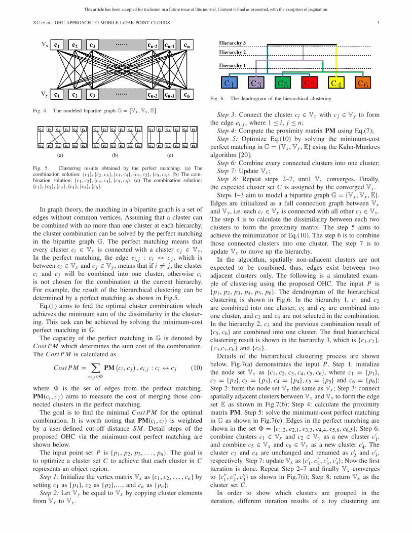
Fig. 6. The dendrogram of the hierarchical clustering.

Step 3: Connect the cluster ci ∈ Vx with c j ∈ Vy to formthe edge ei, j , where 1 ≤ i, j ≤ n;

Step 4: Compute the proximity matrix PM using Eq.(7);Step 5: Optimize Eq.(10) by solving the minimum-cost

perfect matching in G = {Vx , Vy, E} using the Kuhn-Munkresalgorithm [20];

Step 6: Combine every connected clusters into one cluster;Step 7: Update Vx ;Step 8: Repeat steps 2–7, until Vx converges. Finally,

the expected cluster set C is assigned by the converged Vx .Steps 1–3 aim to model a bipartite graph G = {Vx , Vy, E}.

Edges are initialized as a full connection graph between Vx

and Vy , i.e. each ci ∈ Vx is connected with all other c j ∈ Vy .The step 4 is to calculate the dissimilarity between each twoclusters to form the proximity matrix. The step 5 aims toachieve the minimization of Eq.(10). The step 6 is to combinethose connected clusters into one cluster. The step 7 is toupdate Vx to move up the hierarchy.

In the algorithm, spatially non-adjacent clusters are notexpected to be combined, thus, edges exist between twoadjacent clusters only. The following is a simulated exam-ple of clustering using the proposed OHC. The input P is{p1, p2, p3, p4, p5, p6}. The dendrogram of the hierarchicalclustering is shown in Fig.6. In the hierarchy 1, c1 and c2are combined into one cluster, c5 and c6 are combined intoone cluster, and c3 and c4 are not selected in the combination.In the hierarchy 2, c3 and the previous combination result of{c5, c6} are combined into one cluster. The final hierarchicalclustering result is shown in the hierarchy 3, which is {c1,c2},{c3,c5,c6} and {c4}.

Details of the hierarchical clustering process are shownbelow. Fig.7(a) demonstrates the input P . Step 1: initializethe node set Vx as {c1, c2, c3, c4, c5, c6}, where c1 = {p1},c2 = {p2}, c3 = {p3}, c4 = {p4}, c5 = {p5} and c6 = {p6};Step 2: form the node set Vy the same as Vx ; Step 3: connectspatially adjacent clusters between Vx and Vy to form the edgeset E as shown in Fig.7(b); Step 4: calculate the proximitymatrix PM. Step 5: solve the minimum-cost perfect matchingin G as shown in Fig.7(c). Edges in the perfect matching areshown in the set � = {e1,2, e2,1, e3,3, e4,4, e5,6, e6,5}; Step 6:combine clusters c1 ∈ Vx and c2 ∈ Vy as a new cluster c′

1,and combine c5 ∈ Vx and c6 ∈ Vy as a new cluster c′

4. Thecluster c3 and c4 are unchanged and renamed as c′

2 and c′3,

respectively. Step 7: update Vx as {c′1, c′

2, c′3, c′

4}; Now the firstiteration is done. Repeat Step 2–7 and finally Vx convergesto {c′′

1 , c′′2 , c′′

3} as shown in Fig.7(i); Step 8: return Vx as thecluster set C .

In order to show which clusters are grouped in theiteration, different iteration results of a toy clustering are



Fig. 7. A simulated example of the proposed OHC. (a) Initial clusters.(b) The bipartite graph based on (a). (c) The minimum-cost perfect matchingin (b). (d) Cluster sets after the combination based on (c). (e) The bipartitegraph based on (d). (f) The minimum-cost perfect matching in (e). (g) Clustersets after the combination based on (f). (h) The bipartite graph based on (g).(i) The minimum-cost perfect matching in (h).

Fig. 8. The toy example of the proposed OHC. (a) Input pointclouds. (b) Clustering results. (c) Initial input of 680 points. (d) Resultsat the first iteration of 680 clusters. (e) Results at the third iterationof 490 clusters. (f) Results at the fifth iteration of 26 clusters. (g) Resultsat the seventh iteration of 9 clusters. (h) Results at the ninth iteration of2 clusters.

demonstrated in Fig.8. Fig.8(a) and (b) show the inputpoint clouds and results, respectively. Fig.8(c)–(h) show theclose-view of clustering at the iteration #1,#3,#5,#7 and #9,respectively.

The matrix PM after the iteration #7 according to Fig.8(g) isshown in Fig.9(a). The corresponding bipartite graph is shownin Fig.9(b). The achieved minimum-cost perfect matching isshown in Fig.8(c). Based on the connected edges in Fig.8(c),the cluster set C is updated as {c′

1, c′2, c′

3, c′4, c′

5, c′6}, where

c′1 = {c1}, c′

2 = {c2, c3}, c′3 = {c4, c6}, c′

4 = {c5}, c′5 = {c7}

and c′6 = {c8, c9}. In this example, SM is chosen as 0.4.

VI. EXPERIMENTS

A. Evaluation Methods

In the evaluation, the clustering result is C = {c1,c2, . . . , ci , . . . , ct } and the ground truth is C ′ = {c′

1,c′

2, . . . , c′j , . . . , c′

t ′ }. Each ci or c′j means a point cluster and

there are t clusters in C and t ′ clusters in C ′. For the purpose ofevaluating results, we calculate the accuracy assessment ncom

Fig. 9. The proximity matrix at the 7th iteration. (a) The numerical valuesof the proximity matrix. (b) The achieved bipartite graph. (c) The achievedminimum-cost perfect matching.

and ncor as shown in Eq.(11) based on the Jaccard index [21],which commonly used in cluster evaluation.

ncom = 1

t ′t ′∑

j=1

(

tmaxi=1

|c′j

⋂ci |

|c′j |

)

ncor = 1

t

t∑

i=1

(

t ′maxj=1

|ci⋂

c′j |

|ci | ) (11)

The ncom is to measure the completeness ratio between thecorrectly grouped points and the ground truth. The ncor is tomeasure the correctness ratio between the correctly groupedpoints and the hierarchical clustering result. The problem ofEq.(11) is that if there is only one cluster in the ground truthC ′, ncor will be always 1, and if there is only one clusterin the result C , ncom will be always 1. In order to addressthis problem, the minimum of ncom and ncor is chosen asthe accuracy, i.e. nacc = min(ncom, ncor ), to measure points’difference between C and C ′.

B. Comparisons of Different Methods

This section evaluates performances of KMiPC [16],KNNiPC [9], 3DNCut [3], MinCut [4], PEAC [17] and theproposed OHC on five typical scenes. Experimental scenesare shown in Fig.10, including the HouseSet: a single object,the BushesSet: two separated sparse objects, the LamppostSet:two connected rigid objects, the TreesSet: two connectednon-rigid objects and the PowerlinesSet: a complex scenewith different objects. Those experimental scenes are collectedby the mobile laser scanner, i.e. RIEGL VMX-450 sys-tem, which uses a narrow infrared laser beam at a very



Fig. 10. Performances of different methods. (a) HouseSet. (b) BushSet. (c) LamppostSet. (d) TreeSet. (e) PowerlinesSet. Row 1: the segmentation groundtruth of each scene. Row 2: performance of KMiPC [16]. Row 3: performance of KNNiPC [9]. Row 4: performance of 3DNCut [3]. Row 5: performance ofMinCut [4]. Row 6: performance of PEAC [17]. Row 7: performance of the proposed OHC.

high scanning rate. The scanner can be up to 200 lines/secand enables full 360-degree beam deflection without anygaps.

The first row of Fig.10 shows the ground truth. Sincethe ground-truth of object regions is difficult to reproduce,our ground-truth is achieved by segmenting visually inde-pendent object instances manually. We use the CloudCom-pare visualization software (http://www.danielgm.net/cc/) tosegment instance one by one. From the second row to the

last are the performance of KMiPC, KNNiPC, 3DNCut,MinCut, PEAC and the proposed OHC, respectively. In thevisualization, different colors are used to represent differentsegments. KMiPC, KNNiPC and MinCut are implementedby using the Point Cloud Library (www.pointclouds.org/),3DNCut is extended from the normalized-cut method(www.cis.upenn.edu/ jshi/software/). PEAC is achieved basedon the software of Feng et al. (www.merl.com/research/?research=license-request&sw=PEAC).



Fig. 11. Evaluation of different methods using nacc.

KMiPC is suitable for segmenting symmetric objects andworks well in the BushesSet and TreesSet. However, it failsto split connected objects. KNNiPC relies on the densityheavily and is difficult to separate different objects as shownin the HouseSet. 3DNCut tries to normalize the difference ofpoints’ Euclidean distances in each group. It tends to grouppoints evenly as shown in the HouseSet and TreesSet. MinCutperforms well in most cases when the required center pointand radius of each object are set properly. PEAC groups pointsbased on the planar information and requires organizing databefore the segmentation. The proposed OHC is not sensitiveto the density of points as shown in the BushesSet. Moreover,it does not require initial number of clusters and the locationof each object. The attached traffic sign in the LamppostSet issegmented successfully by using the proposed OHC. The splitof the overlapping regions between non-rigid objects is ratherdifficult due to the rapid change of normal vectors as shownin the TreesSet. In the step of computing the normal vectorat a point, when using the normal vectors for the clustering,it makes much different if points are located on a tree. Basedon Eq.(7), we set a large λ to let the Euclidean distancedominate the PM calculation. Results are shown in the lastrow of Fig.10(d). Leaves points are supposed grouped intoone cluster. The over-segmentation is because that there areseparated branches and each tree crown is regarded as onecluster.

The quantitative evaluation is shown in Fig.11. One canobserve that the average accuracy of the proposed OHC ishigher than other methods through all experimental scenes.In the clustering, the proposed OHC uses the matchingin a bipartite graph to combine regions from the sameobject instance, such as the house facade and trash binin Fig.10(a) and Fig.10(c), respectively. The proposed methodachieves the optimal cluster combination by solving theminimum-cost perfect matching in the point-based graph. Thisis more accurate than other methods in splitting of overlappingregions from different instances as shown in Fig.10(b) i.e. thesplit of bushes and ground, Fig.10(d) i.e. the split of trunksand tree leaves, and Fig.10(e) i.e. the split of power-lines andpoles. The key is the proposed combination optimization inthe clustering.

C. Analysis of Parameters Sensitivity

In the implementation of the proposed OHC, there arethree parameters, namely the k to select the nearest neighbor

Fig. 12. Sensitivity analysis. (a) Mean μ is 0.8673, standard deviation σ is0.0107 (fix k = 40 and λ = 4). (b) Mean μ is 0.8595, standard deviation σ is0.0086 (fix λ = 4 and SM = 0.4).(c) Mean μ is 0.8474, standard deviationσ is 0.0132 (fix k = 40 and SM = 0.4).

points, λ to balance the weight of the α(

pi , p j , ci , c j)

andβ


), and SM to formulate the proximity matrix.

In this paper, λ is 4, k is 40 and SM is 0.4. For the purposeof the sensitivity analysis, we range all parameters from -30% to 30% with respect to the above-mentioned values. Thisexperiment is conducted by fixing two parameters among λ,SM and k and alternating the rest one. Fig.12 (a) shows resultsby fixing k = 40 and λ = 4, Fig.12 (b) shows results by fixingλ = 4 and SM = 0.4 and Fig.12 (c) shows results by fixingk = 40 and SM = 0.4. In each case, the mean accuracyis above 85% and the standard deviation is less than 1.5%.A large k or SM may cause under-segmentation and a smallk or SM will increase the over-segmentation rate. A large λworks well for segmenting connected objects and a small λis preferred when there are less overlapping among differentobjects.

Although the proposed OHC requires to be given threeparameters empirically, which can be a shortcoming of ourwork, Fig.12 demonstrates that it is stable to different inputparameters in the suggested value. In the future, we will tryto figure out the adaptive parameter setting method at the riskof requiring more prior knowledge of input scenes.

D. Performance on Large-Scale Datasets

We also test the proposed OHC on two large-scale MLSdatasets. Fig.13 shows the performance on a large-scale resi-dential point set (558 MB, 12,551,837 points) scanned by the



Fig. 13. Clustering results of a large-scale residential point set.

Fig. 14. Clustering results of a large-scale urban point set.

RIEGL scanner. Fig.14 shows results of a large-scale urbanpoint set (528 MB, 10,870,886 points) collected by the Optechscanner.

Segmentation challenges in the residential point set are(1) the split of overlapping trees and (2) the split of houseswith different structures. As shown in Fig.13, we succeed toseparate trees and houses into different clusters in region A.A house instance is split into several regions as shown inregion B. Segmentation challenges in the urban point set arethe split of objects with varied sizes. Various high buildingsand low vegetation are segmented as shown in Fig.14 region A.A high building is separated from the base, because of thedata incompleteness in connectivity regions as shown in Fig.14region B.

Both 3DNCut and MinCut require human-computer interac-tion in the point cloud segmentation, for example, they requirepresetting the number of objects in the scene. The MinCutrequires manually setting center points and radius for eachobject, which is extremely time-consuming in the large-scalescenes. PEAC is proposed for dealing with organized pointclouds. Therefore, it is not practical to test 3DNCut, MinCutand PEAC on large-scale scenes.

VII. DISCUSSION

A. Merging Regions

Since our clustering results can not be used in the objectdetection or recognition, we propose a merging strategy tocombine regions into object instances. The expected outcomeis that after the rule-based merging process, regions from thesame object are combined into one instance. In this paper,we merge regions using the following two rules.

(1) The first rule is based on Euclidean distances betweenclusters. With the help of the ground information in MLS

Fig. 15. Merging results based on the Euclidean distance.

Fig. 16. Merging results based on the subset information.

data demonstrated in the left of Fig.15, we can easily obtainroad direction in a local region (i.e. 10 m by 10 m). Whencalculate Euclidean distances between the point pi and p j ,if the direction from pi to p j is parallel to the local roaddirection, d(pi , p j ) will be enlarged by 5 times. This ruleis designed for the distance calculation in the XOY plane.It is worth noting that spatially close clusters are merged intoone component in the above-mentioned clustering process.Therefore, we increase the Euclidean distance threshold inthe merging of regions. If the closest distance between twoclusters is less than 5 m, they will be merged into one cluster.This rule works well in merging houses, vehicles and trees asshown in the right of Fig.15.

(2) The second rule is based on the subset information.As shown in the left of Fig.16, the cluster A and B areneighbors in the Z-axis direction. A′ and B ′ are projectionpoint sets of the cluster A and B in the XOY plane, receptively.If |A′∩B ′|

|A′ | > 0.9 (i.e. A′ ⊂ B ′) or |A′∩B ′||B ′| > 0.9 (i.e. B ′ ⊂ A′),

the cluster A and B will be merged into one cluster AB . Thisrule is designed for merging clusters in the Z direction, suchas roofs and facades as shown in the right of Fig.16.

We use the above-mentioned rules one-by-one in the auto-matic merging process. The merging results of the aboveresidential and urban scenes are shown in Fig.17 and Fig.18,respectively. Each bounding box indicates an object instanceafter the rule-based merging process. Fig.17 region A demon-strates the merging of trees and Fig.17 region B shows themerging of houses. Fig.18 region A demonstrates the mergingof buildings and Fig.18 region B shows the merging ofbuildings. Regions from one object are merged into the sameinstance.



Fig. 17. Merging performance on residential scene.

Fig. 18. Merging performance on urban scene.

TABLE I

EXECUTION TIME OF EACH ALGORITHM

B. Complexity Analysis

The proposed OHC works automatically for the point cloudclustering. There is no need for human-computer interaction,e.g. set initial number of clusters or locations of each object.The performance is competitive against the state-of-the-artmethods.

The space complexity of the initial proximity matrixis O(N2). Since the proximity matrix is symmetric andmost of its elements are ∞, we use sparse matrix strategyto reduce the space complexity. The time complexity relieson the Kuhn-Munkres algorithm which is O(N2). To dealwith the large-scale point cloud clustering, we present astrategy to increase our efficiency: 1) remove ground points

Fig. 19. Ground removal. (a) Input scene. (b) Ground points.(c) Above-ground points.

using the Cloth Simulation Filter (CSF) approach [22];2) down-sample the above-ground points into a sparse pointby randomly removing points from input data; 3) apply the



Fig. 20. Clustering results from down-sampled points. The first row shows input down-sampled data and the second row shows our results. (a) Pointsare down-sampled to 90%. (b) Points are down-sampled to 60%. (c) Points are down-sampled to 30%. (d) Points are down-sampled to 10%. (e) Points aredown-sampled to 5%. (f) Points are down-sampled to 1%.

TABLE II

ANALYSIS OF THE SEGMENTATION FROM DOWN-SAMPLED POINTS

proposed OHC to the down-sampling data; 4) assign those dis-carded points from the down-sampling process to their closestclusters.

The cost time in each algorithm is shown in Table.I. In thecomparison, only KMiPC and KNNiPC perform better thanours. 3DNCut is slower than the proposed method when thescale of the scene is large. For MinCut, the human-computerinteraction is very time-consuming. The organization of pointclouds in PEAC is not counted in Table.I, which will costlots of time. In order to deal with the high complexity issue,Fig.19 shows the performance of OHC on down-samplingdata. Fig.19 (a) shows an input scene containing vegetation,buildings and roads. Ground are removed by the CSF approachas shown in Fig.19 (b). The rest of above-ground points areshown in Fig.19 (c) which are down-sampled to different levelsrandomly. The first row of Fig.20 demonstrates down-sampledpoints by 90%, 60%, 30%, 10%, 5% and 1%. The secondrow of Fig.20 shows the corresponding object segmentationresults.

In the case of inputting down-sampling data, althoughthe accuracy of the overlapping region segmentation isdecreased and there appear the over-segmentation andunder-segmentation as shown in Fig.20 and Table II, OHCprovides promising results at different sampling levels. Theaccuracy and cost time are shown in Table II. This exper-iment was done on a Windows 10 Enterprise 64-bit, IntelCore i7-6900k 3.20GHz processor with 64 GB of RAM byusing Matlab R2018a. By using the down-sampling strategy,the proposed OHC succeeds in segmenting objects from alarge-scale point set effectively.

VIII. CONCLUSIONS

This paper investigates a new optimal hierarchical clus-tering (OHC) method for achieving object instances from3D mobile LiDAR point clouds. The cluster combination isobtained by the matching in a point-based graph, and thecombination is optimized by solving the minimum-cost perfectmatching in a bipartite graph. In the sensitivity analysis,the standard deviation of the accuracy is less than 1.5%through all experimental scenes, which shows the algorithm’srobustness to different parameters. To merge regions intoobject instances, this work proposes a rule-based groupingstrategy to merge regions into the same object. The draw-back of the proposed OHC is the time complexity, whichis addressed by using the sampling strategy. Performance onthe residential and urban point sets shows that the proposedmethod is effective in clustering regions from different scenesand superior to the state-of-the-art methods in terms of theaccuracy.

Future work will focus on adding the dissimilarity measureof the intensity and color information in the proximity matrix.Besides, we will try to improve the efficiency of the combi-nation by using supervoxel techniques in the clustering.

REFERENCES

[1] H. Wang, C. Wang, H. Luo, P. Li, Y. Chen, and J. Li, “3-D point cloudobject detection based on supervoxel neighborhood with Hough forestframework,” IEEE J. Sel. Topics Appl. Earth Observ. Remote Sens.,vol. 8, no. 4, pp. 1570–1581, Apr. 2015.

[2] L. Nan and P. Wonka, “PolyFit: Polygonal surface reconstruction frompoint clouds,” in Proc. IEEE Conf. Comput. Vis. Pattern Recognit.,Oct. 2017, pp. 2353–2361.

[3] Y. Yu, J. Li, H. Guan, C. Wang, and J. Yu, “Semiautomated extractionof street light poles from mobile LiDAR point-clouds,” IEEE Trans.Geosci. Remote Sens., vol. 53, no. 3, pp. 1374–1386, Mar. 2014.

[4] A. Golovinskiy, V. G. Kim, and T. Funkhouser, “Shape-based recogni-tion of 3D point clouds in urban environments,” in Proc. IEEE 12th Int.Conf. Comput. Vis., Sep./Oct. 2009, pp. 2154–2161.

[5] Y. Zhang, J. Wang, X. Wang, and J. M. Dolan, “Road-segmentation-based curb detection method for self-driving via a 3D-LiDAR sensor,”IEEE Trans. Intell. Transp. Syst., vol. 19, no. 12, pp. 3981–3991,Dec. 2018.

[6] K. Li, X. Wang, Y. Xu, and J. Wang, “Density enhancement-based long-range pedestrian detection using 3-D range data,” IEEE Trans. Intell.Transp. Syst., vol. 17, no. 5, pp. 1368–1380, May 2016.



[7] F. Wu et al., “Rapid localization and extraction of street light polesin mobile LiDAR point clouds: A supervoxel-based approach,” IEEETrans. Intell. Transp. Syst., vol. 18, no. 2, pp. 292–305, Feb. 2017.

[8] P. Corcoran, A. Winstanley, P. Mooney, and R. Middleton, “Backgroundforeground segmentation for SLAM,” IEEE Trans. Intell. Transp. Syst.,vol. 12, no. 4, pp. 1177–1183, Dec. 2011.

[9] B. Douillard et al., “On the segmentation of 3D LIDAR pointclouds,” in Proc. IEEE Int. Conf. Robot. Automat. (ICRA), May 2011,pp. 2798–2805.

[10] K. Klasing, D. Wollherr, and M. Buss, “A clustering method forefficient segmentation of 3D laser data,” in Proc. ICRA, May 2008,pp. 4043–4048.

[11] J. Shi and J. Malik, “Normalized cuts and image segmentation,”IEEE Trans. Pattern Anal. Mach. Intell., vol. 22, no. 8, pp. 888–905,Aug. 2000.

[12] Y. Boykov and G. Funka-Lea, “Graph cuts and efficient N-D imagesegmentation,” Int. J. Comput. Vis., vol. 70, no. 2, pp. 109–131, 2006.

[13] Y.-T. Su, J. Bethel, and S. Hu, “Octree-based segmentation forterrestrial LiDAR point cloud data in industrial applications,”ISPRS J. Photogramm. Remote Sens., vol. 113, pp. 59–74, Mar. 2016.

[14] Y. Lin, C. Wang, D. Zhai, W. Li, and J. Li, “Toward betterboundary preserved supervoxel segmentation for 3D point clouds,”ISPRS J. Photogramm. Remote Sens., vol. 143, pp. 39–47, Sep. 2018.

[15] G. Lavoué, F. Dupont, and A. Baskurt, “A new CAD mesh segmenta-tion method, based on curvature tensor analysis,” Comput.-Aided Des.,vol. 37, no. 10, pp. 975–987, 2005.

[16] R. A. Kuçak, E. Özdemir, and S. Erol, “The segmentation ofpoint clouds with k-means and ann (artifical neural network),” Int.Arch. Photogramm., Remote Sens. Spatial Inf. Sci., vol. XLII-1/W1,pp. 595–598, Jun. 2017. [Online]. Available: http://www.int-arch-photogramm-remote-sens-spatial-inf-sci.net/XLII-1-W1/595/2017/

[17] C. Feng, Y. Taguchi, and V. R. Kamat, “Fast plane extraction inorganized point clouds using agglomerative hierarchical clustering,”in Proc. IEEE Int. Conf. Robot. Automat. (ICRA), May/Jun. 2014,pp. 6218–6225.

[18] D. Chaudhuri and B. B. Chaudhuri, “A novel multiseed nonhierarchicaldata clustering technique,” IEEE Trans. Syst., Man, Cybern. B, Cybern.,vol. 27, no. 5, pp. 871–876, Sep. 1997.

[19] H. Edelsbrunner, D. G. Kirkpatrick, and R. Seidel, “On the shape ofa set of points in the plane,” IEEE Trans. Inf. Theory, vol. 29, no. 4,pp. 551–559, Jul. 1983.

[20] J. Munkres, “Algorithms for the assignment and transportation prob-lems,” J. Soc. Ind. Appl. Math., vol. 5, no. 1, pp. 32–38, 1957.

[21] G. W. Milligan and M. C. Cooper, “A study of the comparability ofexternal criteria for hierarchical cluster analysis,” Multivariate Behav.Res., vol. 21, no. 4, pp. 441–458, 1986.

[22] W. Zhang et al., “An easy-to-use airborne LiDAR data filtering methodbased on cloth simulation,” Remote Sens., vol. 8, no. 6, p. 501,Jun. 2016.

Sheng Xu received the B.Eng. degree in computerscience and technology from Nanjing Forestry Uni-versity and the Ph.D. degree in digital image systemsfrom the University of Calgary. In 2018, he joinedthe College of Information Science and Technology,Nanjing Forestry University, where he is currentlyan Assistant Professor. His current research interestsinclude mobile mapping, vegetation mapping, andcomputer vision.

Ruisheng Wang received the B.Eng. degree inphotogrammetry and remote sensing from WuhanUniversity, the M.Sc.E. degree in geomatics engi-neering from the University of New Brunswick,and the Ph.D. degree in electrical and computerengineering from McGill University. He has beenan Industrial Researcher with Nokia, Chicago, IL,USA, since 2008. In 2012, he joined the Departmentof Geomatics Engineering, University of Calgary,where he is currently an Associate Professor. He hasalso been a Distinguished Professor of Geographical

Sciences at Guangzhou University. His research interests include geomaticsand computer vision.

Hao Wang received the B.Eng. degree from Nan-jing Forestry University and the Ph.D. degree fromTongji University. In 1983, he joined the Col-lege of Landscape Architecture, Nanjing ForestryUniversity, where he is currently a Professor. Hisresearch interests include landscape architecturedesign, urban planning, and green space systemAnalysis. He is a member of the Editorial Committeeof the Chinese Landscape Architecture.

Han Zheng received the B.S. and M.S. degreesin geodesy and geomatics engineering from WuhanUniversity, Wuhan, China, in 2011 and 2013, respec-tively. He is currently pursuing the master’s degreein digital image system with the Department of Geo-matics Engineering, University of Calgary, Calgary,AB, Canada. His current research interests includelaser measurement application, computer vision, dig-ital image processing, and object recognition fromthree-dimensional point clouds.

Documents

An Optimal Hierarchical Clustering Approach to Mobile