An Optimal Constraint Programming Approach to theOpen-Shop Problem

Arnaud MalapertÉcole des Mines de Nantes, LINA UMR CNRS 6241, Nantes, France

École Polytechnique de Montréal, CIRRELT, Montréal, Québec, Canadaarnaud.malapert@mines-nantes.fr

Hadrien CambazardCork Constraint Computation Centre, Department of Computer Science, University College Cork, Ireland

Christelle GuéretÉcole des Mines de Nantes, IRCCyN UMR CNRS 6597, Nantes, France

Narendra JussienÉcole des Mines de Nantes, LINA UMR CNRS 6241, Nantes, France

André Langevin, Louis-Martin RousseauÉcole Polytechnique de Montréal, CIRRELT, Montréal, Québec, Canada

This paper presents an optimal constraint programming approach for the Open-Shop schedul-ing problem, which integrates recent constraint propagation and branching techniques withnew upper bound heuristics. Randomized restart policies combined with nogood recordingallow to search diversification and learning from restarts. This approach is compared withthe best-known metaheuristics and exact algorithms, and shows better results on a widerange of benchmark instances.

Key words: Production-Scheduling, Open shop; Computers-computer science: Artificial In-telligence; Constraint Programming; Randomization and Restart

1. IntroductionOpen-Shop problems are at the core of many scheduling problems involving unary resourcessuch as Job-Shop or Flow-Shop problems, which have received an important amount ofattention because of their wide range of applications. Among the many techniques proposedin the literature, Constraint Programming (CP) is among the most successful.

In the Open-Shop problem (OSP), a set J of n jobs, consisting each of m tasks (oroperations), must be processed on a set M of m machines. The processing times are givenby a matrix P : m× n, in which pij ≥ 0 is the processing time of task Tij ∈ T of job Jj, tobe done on machine Mi. The tasks of a job can be processed in any order, but only one at atime. Similarly, a machine can process only one task at a time. We consider the constructionof non-preemptive schedules of minimal makespan Cmax, which is NP-Hard for m ≥ 3 (seeGonzalez and Sahni, 1976). Figure 1 shows an optimal solution of the problem where eachline/shade represents a machine/job.A classical lower bound CLB

max for this problem is equal to the maximum workload over everymachine and every job given by: max

(max1≤i≤m(∑n

j=1 pij),max1≤j≤n(∑mi=1 pij)

). Three sets

of benchmark instances are available in the literature (Taillard, 1993; Brucker et al., 1997;Guéret and Prins, 1999).

1

GP03-02 - Cmax=1170

0 100 200 300 400 500 600 700 800 900 1 000 1 100 1 200

Time

M_0

M_1

M_2

Res

ou

rces

T_2_0 T_2_1T_2_2

T_1_1 T_1_2

T_0_0 T_0_1T_0_2

Figure 1: An optimal solution of the instance GP03-02 with makespan equal to 1170.

The first exact method (Brucker et al., 1996) proposed for the Open-Shop problem isbased on the resolution of a one-machine problem with positive and negative time lags. Thesecond one (Brucker et al., 1997) consists of fixing precedences on the critical path of heuris-tic solutions computed at each node. Although that last method is efficient, some problemsof Taillard benchmark from size 7× 7 remained unsolved.Guéret et al. (2000) proposed an intelligent backtracking technique applied to the Bruckerbranching scheme. When a contradiction is raised during search, instead of systematicallybacktracking to the previous decision (chronological backtracking), the algorithm analyzesthe reasons for the contradiction to avoid questioning decisions that are not related to thefailure, and backtracks to a more relevant choice point. This approach significantly reducesthe number of backtracks, but can consume twice the CPU time in each node. They furtherapplied additional search tree reduction based on forbidden intervals, i.e. time intervals inwhich no operation can start or end in an optimal solution (Guéret and Prins, 1998).Dorndorf et al. (2001) improved the Brucker algorithm by using consistency techniques.Instead of analyzing and improving the search strategies, they focused on constraint prop-agation techniques for reducing the search space. Furthermore, they studied top-down andbottom-up optimization procedures depending on the average workload of a problem instance.The top-down procedure starts with a upper bound ub and tries to improve it. The bottom-up procedure starts with a lower bound lb as target upper bound which is incremented byone unit until the problem becomes feasible. Their algorithms were the first to solve manyproblem instances to optimality in a short amount of time. However, some problems of Tail-lard benchmark from size 15 × 15 remained unsolved, as well as some of Brucker instancesfrom size 7× 7.More recently, Laborie (2005) proposed a bottom-up search for cumulative scheduling basedon the detection ofMinimal Critical Sets (MCS) and advanced propagation with self-adaptedshaving. A MCS is a minimal set of resource requirements on the same resource that wouldover-consume the resource if executed simultaneously. A heuristic selects critical sets by

2

estimating the related reduction of the search space. The approach closed the 34 remainingopen instances of Guéret-Prins benchmark and 3 of the 6 open instances of Brucker bench-mark.Most bottom-up variants differ by the way infeasibilities are resolved. Dichotomous variantsresolve infeasibilities by repeatedly dividing the makespan interval [lb, ub[ in half until itbecomes empty. If the subproblem [lb,

⌈lb+ub

2

⌉[ is feasible, then the current makespan pro-

vides a new upper bound. Otherwise, the value⌈lb+ub

2

⌉is a new legal lower bound. As a

consequence, these variants begin with a legal lower bound and an initial feasible solution.For instance, the first branch of the first iteration can provide an initial solution if no initialconstraint on the makespan is stated. In practice, it is often important to guarantee thelength of the initial interval since the number of subproblems depends on it. Therefore,another approach consists in increasing the target lower bound by 2k from the previouslystored lower bound at the k-th iteration until finding a solution which provides the ini-tial interval [2k, ub[⊆ [2k, 2k+1[. Dichotomous variants reduce the number of iterations fromCmax − CLB

max + 1 to O(log2

(Cmax − CLB

max + 1)).

Later, Tamura et al. (2006) applied a method to Open-Shop problems that encodes Con-straint Satisfaction/Optimization problems with integer linear constraints into a BooleanSatisfiability Testing problem (SAT). A comparison x ≤ a is encoded by a different booleanvariable for each integer variable x and each integer value a. Then, a simple constraintmodel with deadline constraints and binary disjunctive constraints between two activitiesbelonging to the same job or machine is encoded as a SAT. They proved optimal results forall instances including the last three open instances of Brucker benchmark.

Many metaheuristics algorithms have been developed in the last decade to solve theOpen-Shop problem. The most recent and successful metaheuristics are: Genetic Algo-rithm (Prins, 2000), Construction and Repair (Chatzikokolakis et al., 2004), Ant ColonyOptimization (Blum, 2005) and Particle Swarm Optimization (Sha and Hsu, 2008).Prins (2000) presents several specialized OSP genetic algorithms with two key features: apopulation in which each individual has a distinct makespan, and a special procedure whichreorders every new chromosome.Chatzikokolakis et al. (2004) proposed a general repair operator based on local search tech-niques with a general cost function for evaluating partial assignments. Experimental resultsimproved many best-known solutions of the Guéret-Prins instances.The basic component of Ant Colony Optimization (ACO) is a probabilistic solution con-struction mechanism. Because of its constructive nature, it can be regarded as a tree searchmethod. Based on this observation, Blum (2005) hybridizes the solution construction mech-anism with beam search. Beam search algorithms are incomplete derivatives of branch-and-bound algorithms. It is an approximate method where a partial assignment is only extendedin a restricted number of ways (this limit is called the beam width). The approach improvedon the results obtained by the current best standard ACO algorithms.Particle Swarm Optimization (PSO) is a population-based optimization algorithm, whereeach particle is an individual solution, and the swarm is composed of many particles. Shaand Hsu (2008) modify the representation of particle position, particle movement, and parti-cle velocity to better fit to the OSP. They obtained many optimal solutions to the benchmarkproblems.

3

Finally, many heuristic methods quickly provide good solutions. Most of them are con-structive methods and belong to three main families: priority dispatching rules, matchingalgorithms (see Guéret, 1997), and insertion and appending procedures combined with beamsearch (see Bräsel et al., 1993).

In this paper, we investigate the enhancements of top-down algorithms for Open-Shopproblems as it is important, in practice, to quickly provide good solutions. Our approachrelies on the use of strong propagation mechanisms of the unary resource and temporal con-straint network constraints but also reasoning dedicated to the minimization of the makespansuch as the forbidden intervals method. Our main contribution is to show that randomiza-tion and restart strategies combined with strong propagation and scheduling heuristics canlead to a very efficient approach for solving Open-Shop problems. The proposed solvingtechnique outperforms other approaches published so far on a wide range of benchmarks.This paper is organized as follows. Section 2 introduces our constraint model and Section 3describes techniques that enhance the search of our top-down algorithm. Finally, Section 4presents the experimental results we obtained and investigates the effect of each componentof the algorithm as well as the comparison against other approaches.

2. The Constraint Programming ModelConstraint programming techniques have been widely used to solve scheduling problems.A Constraint Satisfaction Problem (CSP) consists of a set V of variables defined by a cor-responding set of possible values (the domains D) and a set C of constraints. A solutionof the problem is an assignment of a value to each variable such that all constraints aresimultaneously satisfied. Constraints are handled through a propagation mechanism whichallows the reduction of the domains of variables and the pruning of the search tree. Thepropagation mechanism coupled with a backtracking scheme allows the search space to beexplored in a complete way. Scheduling is probably one of the most successful areas forCP thanks to specialized global constraints, which allow modelling resource limitations andtemporal constraints.

Constraint programming models in scheduling usually represent a non-preemptive taskTij by a triplet of non-negative integer variables (sij, pij, eij) denoting the start, processingtime and end of the task such that sij + pij = eij. In Open-Shop problems, the durationpij is known in advance and is a constant. The head of a task estij = inf(sij), denotes itsearliest possible starting time, whereas its tail lctij = sup(eij) is its latest completion time.

In this section, we present our constraint programming model to tackle Open-Shop prob-lems. First, we present the unary resource global constraint which models the fact that asingle machine or job can be processed at any given time. Then, we explain how precedenceconstraints are tackled in the decision and propagation process. We also state additionaldedicated constraints such as forbidden intervals and symmetry breaking constraints. Finally,various branching schemes in constraint-based scheduling are detailed.

4

2.1. Unary ResourceA unary resource constraint, also called disjunctive, models a resource of unit capacity. Theconstraint holds if all the tasks of a collection that have a duration strictly greater than 0do not overlap. One unary resource constraint is stated for each job and each machine. LetT denote a set of tasks sharing a unary resource and Ω denote a subset of T . We considerthe three following propagation rules:

Not First/Not Last: This rule determines if task i cannot be scheduled after or before a setof tasks Ω. In other words, it implies that i cannot be last or first in the set Ω∪i. Inthat case, at least one task from the set must be scheduled after (resp. before) activityi and the tail (resp. head) of i can be updated accordingly.

Edge Finding: This filtering technique determines that some task must be executed first orlast in a set Ω. It is the counterpart of Not First/Not Last.

Detectable Precedence: A precedence i ≺ j (see Section 2.2) is called detectable if it can bediscovered only by comparing the time bounds of its two tasks. Heads and tails of eachtask can then be updated more accurately by the knowledge of all its predecessors orsuccessors.

Several propagation algorithms (Carlier and Pinson, 1994; Caseau and Laburthe, 1995; Bap-tiste and Le Pape, 1996; Vilím, 2004) exist for these rules and the best of them have acomplexity of O(n log(n)). These rules rely on the computation of the Earliest CompletionTime (ECTΩ) of a set of tasks Ω ⊆ T . By denoting estΩ = minTij∈Ωestij, its earliestcompletion time is given by: ECTΩ = maxestΩ′ + ∑

Ω′ pij, Ω′ ⊆ Ω. We chose the imple-mentation proposed by Vilím (2004) that relies on two efficient data structures: Θ-tree andΘ-Λ-tree. These structures are based on a balanced binary tree and allow a quick computa-tion of ECTΩ, especially at each addition or removal of a task in the set.We also take advantage of the computation of ECTΩ to estimate a lower bound of themakespan. In fact, the earliest completion time of a machineMi (resp. a job Jj) is estimatedby the value of ECTMi

(resp. ECTJj). Thereby, the makespan is greater than the maximum

of the earliest completion times among all resources (jobs and machines).

2.2. Temporal ConstraintsThis section deals with the problem of managing quantitative temporal networks withoutdisjunctive constraints. Of course, temporal constraints could be handled by simply addingthe corresponding elementary constraints to the solver and by propagating them indepen-dently. But, some efficient procedures are dedicated to this problem, known as the SimpleTemporal Problem (see Dechter, 2003). This problem involves a set of temporal integervariables X1, . . . , Xn and a set of temporal constraints aij ≤ Xj − Xi ≤ bij, wherebij ≥ aij ≥ 0. Cesta and Oddi (1996) proposed algorithms to manage temporal informa-tion that: (a) allow dynamic changes of the constraint set for both posting and retraction(b) exploit the temporal constraint network for incremental propagation and cycle detection.

Let Tij ≺ Tkl denote a precedence constraint, i.e. a temporal constraint such that sij +pij ≤ skl. A directed graph G = (V,E) is associated with these constraints where the set

5

of nodes V represents the set of tasks and the set of arcs represents the set of precedenceconstraints. Two fictitious tasks Tstart and Tend referring to the starting and ending tasks ofthe schedule, are added to V . An arc is added in E between two tasks Tij and Tkl, if Tijprecedes Tkl (Tij ≺ Tkl). Initially, the only arcs of E are the ones originating at node Tstartor ending at node Tend.

The structure efficiently handles arc insertions/removals and is restorable upon back-tracking, i.e. it maintains a stack to record when a change is done on the graph. Cycleand transitive arc detections have a constant time complexity as we maintain the transitiveclosure of G. Frigioni et al. (2001) proposed an algorithm for maintaining the transitiveclosure information in a directed graph which requires O(n) amortized time for a sequenceof insertions and deletions. In addition, we also maintain a topological order with the sim-ple and efficient algorithm proposed by Pearce and Kelly (2006). Note that, the transitiveclosure information reduces the overall complexity to maintain a topological order.

The branching strategy (see Section 2.4) adds arcs between tasks sharing a unary resourceuntil all these pairs are connected by a path. At the end of the search, the makespan Cmaxof a schedule is the length of a longest path between Tstart and Tend, i.e. a critical path. Thebranching strategy exploits the transitive closure to avoid creating cycles in the networkor branching on transitive or satisfied precedences. Indeed, the precedence network G isconsistent if and only if it does not have any cycle. Then, a precedence can be easilydetected when it is inferred by the bounds of the tasks, but it is not necessarily the case fortransitive precedences. Since precedences satisfy the triangular inequality, if an arc (Tij, Tkl)is transitive, i.e. Tij and Tkl are connected by a path in E\(Tij, Tkl), then the precedenceTij ≺ Tkl can be inferred.

Propagation of a set of precedences can be done in linear time, but a bad orderingof awakes in the propagation loop can lead, in the worst case, to quadratic time beforereaching the fixpoint. Indeed, the longest path from Tstart to Tij, and from Tij to Tend arecomputed to update the head and tail of Tij. Since G is a directed acyclic graph, all longestpaths originating from Tstart and ending at Tend are computed in a linear time with anincremental version of the Dynamic Bellman algorithm for the Single Source Longest Pathproblem (Gondran and Minoux, 1984). A topological order is an input of the algorithm andour implementation avoids redundant computations by maintaining a dynamic topologicalorder. At each propagation, the algorithm considers only a subgraph of G inferred from tasksfor which heads or tails have changed since the last call. Note that the general algorithmproposed by Cesta and Oddi (1996) has a O(|V | × |E|) complexity whereas our algorithm isO(|E|).

2.3. Additional ConstraintsIn this section, we introduce additional constraints that improve the propagation by con-sidering makespan minimization and basic symmetries. These redundant constraints aredominance rules that are not mandatory for the model’s correctness, but improve its resolu-tion. They can be propagated in constant time during the search contrary to complex lowerbounds or dominance rules used in other branching schemes (Brucker et al., 1999), as forinstance the Brucker branching scheme.

6

Forbidden Intervals Forbidden intervals are a specialized filtering technique for OSP withminimal makespan. Forbidden intervals are intervals in which in an optimal solution, taskscan neither start nor end. Heads and tails can be strengthened based on this informationduring search. When the head of a task is in such an interval, it can be increased to theupper bound of the interval. This technique has been proposed by Guéret and Prins (1998)and the computation of forbidden intervals is based on the resolution of m+ n Subset SumProblems. The Subset Sum Problem has an O(d× n) complexity where d is the capacity ofthe knapsack, i.e. the maximal makespan (see Kellerer et al., 2004). Since these problemsare solved once and for all at the beginning of the search, heads and tails are updated in aconstant time.

Symmetry Breaking Many constraint satisfaction problems contain symmetries makingmany solutions equivalent. Symmetry breaking techniques avoid redundant search effort, bytrying to ensure that whenever a partial assignment is shown to be inconsistent, no symmetricassignment is ever tried. A solution of the OSP can be reversed considering the last taskof a machine as the first, the second to last task as the second and so on. This symmetriccounterpart of any solution is also a solution for the OSP. Once the algorithm has proventhat one ordering of the tasks is suboptimal, it is unnecessary to check the reverse ordering.Breaking this symmetry can be done by choosing any task Tij and a priori imposing that itstarts in the first half of the schedule: sij ≤

⌈eend−pij

2

⌉. Our algorithm selects the task with

the longest processing time.

2.4. Branching SchemeBranching strategies in scheduling can be divided into two main families: assigning startingtimes or fixing precedences. The former leads to n-ary branching schemes whereas the latteryields binary decisions.

In the first family, the most well-known strategy is referred to as setTimes (Le Papeet al., 1994) and is an incomplete branching scheme. However, SetTimes is complete inmany specific applications including shop problems. At each node, it selects a task froma set of unscheduled and selectable tasks, creates a choice point and schedules the selectedtask at its earliest starting time. Upon backtracking, it labels the task that was scheduledat the considered choice point as not selectable, as long as its earliest start has not changed.

The second family consists of fixing precedences between tasks. The n-ary branchingof Brucker et al. (1997) (denoted as Block) is based on the computation of one heuristicsolution at each node to decide which precedences to enforce. The tasks along the criticalpath of this heuristic solution are selected and precedences are stated to question the cur-rent critical path. This branching scheme can fix many precedences simultaneously whileremaining complete.Beck et al. (1997) proposed a simpler binary branching scheme (denoted as Profile) wheretwo critical tasks sharing the same unary resource are ordered. The individual demand is(probabilistically) the amount of a resource required by the activity at time t. To estimatecontention, the individual demands of each task are aggregated for each resource by sum-ming the individual demand curves for that resource. This aggregate demand curve is usedas a measure of the contention for the resource over time. At each node, the resource and

7

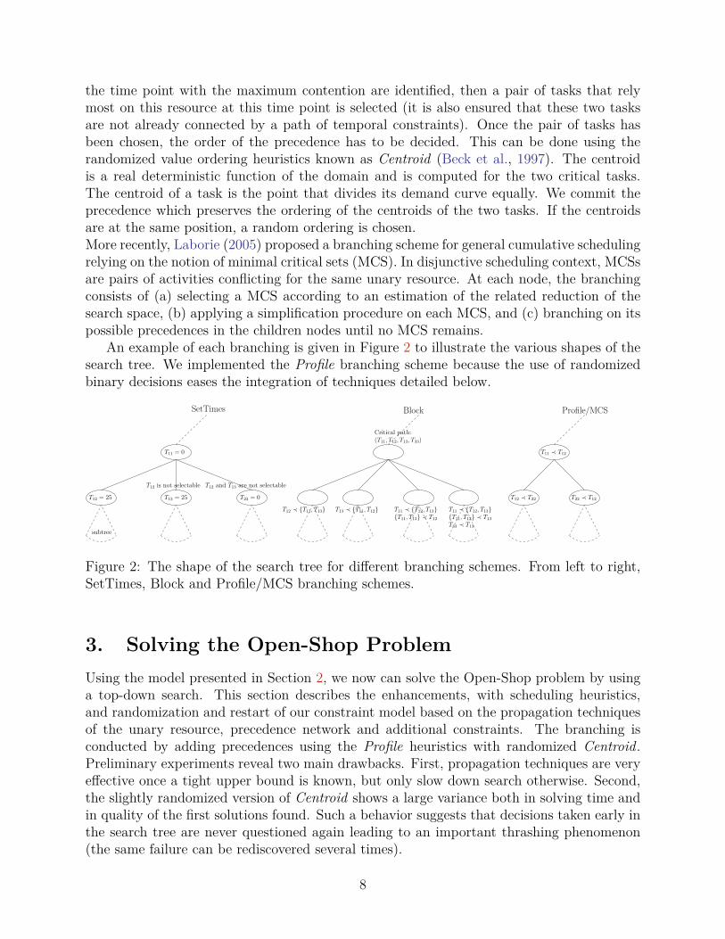
the time point with the maximum contention are identified, then a pair of tasks that relymost on this resource at this time point is selected (it is also ensured that these two tasksare not already connected by a path of temporal constraints). Once the pair of tasks hasbeen chosen, the order of the precedence has to be decided. This can be done using therandomized value ordering heuristics known as Centroid (Beck et al., 1997). The centroidis a real deterministic function of the domain and is computed for the two critical tasks.The centroid of a task is the point that divides its demand curve equally. We commit theprecedence which preserves the ordering of the centroids of the two tasks. If the centroidsare at the same position, a random ordering is chosen.More recently, Laborie (2005) proposed a branching scheme for general cumulative schedulingrelying on the notion of minimal critical sets (MCS). In disjunctive scheduling context, MCSsare pairs of activities conflicting for the same unary resource. At each node, the branchingconsists of (a) selecting a MCS according to an estimation of the related reduction of thesearch space, (b) applying a simplification procedure on each MCS, and (c) branching on itspossible precedences in the children nodes until no MCS remains.

An example of each branching is given in Figure 2 to illustrate the various shapes of thesearch tree. We implemented the Profile branching scheme because the use of randomizedbinary decisions eases the integration of techniques detailed below.

T11 = 0

T12 = 25 T13 = 25 T23 = 0

T12 is not selectable

Critical path:

T12 ≺ T11, T13

SetTimes

subtree

T12 and T13 are not selectable

Block Profile/MCS

(T11, T12, T13, T33)

T13 ≺ T11, T12T11, T13 ≺ T12 T11, T12 ≺ T13

T11 ≺ T12, T13

T33 ≺ T13

T11 ≺ T12, T13

T12 ≺ T22 T22 ≺ T12

T11 ≺ T12

Figure 2: The shape of the search tree for different branching schemes. From left to right,SetTimes, Block and Profile/MCS branching schemes.

3. Solving the Open-Shop ProblemUsing the model presented in Section 2, we now can solve the Open-Shop problem by usinga top-down search. This section describes the enhancements, with scheduling heuristics,and randomization and restart of our constraint model based on the propagation techniquesof the unary resource, precedence network and additional constraints. The branching isconducted by adding precedences using the Profile heuristics with randomized Centroid.Preliminary experiments reveal two main drawbacks. First, propagation techniques are veryeffective once a tight upper bound is known, but only slow down search otherwise. Second,the slightly randomized version of Centroid shows a large variance both in solving time andin quality of the first solutions found. Such a behavior suggests that decisions taken early inthe search tree are never questioned again leading to an important thrashing phenomenon(the same failure can be rediscovered several times).

8

We propose to apply a randomized constructive heuristic (without propagation) whichinitializes the upper bound so that the selection and propagation of initial choices is improvedat the beginning of the complete search. Furthermore, we propose a restarting strategyenhanced with nogood recording at each restart to prevent exploring the same part of thesearch space again. Note that these two techniques can be used in any top-down approachand with any branching scheme, although recording nogoods is made easier by using binarydecisions. We now give a detailed presentation of the overall approach and analyze itsparameters.

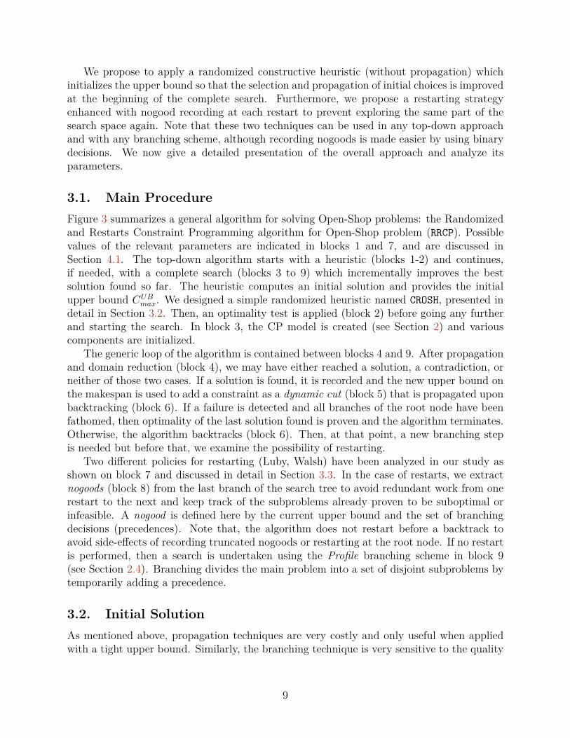
3.1. Main ProcedureFigure 3 summarizes a general algorithm for solving Open-Shop problems: the Randomizedand Restarts Constraint Programming algorithm for Open-Shop problem (RRCP). Possiblevalues of the relevant parameters are indicated in blocks 1 and 7, and are discussed inSection 4.1. The top-down algorithm starts with a heuristic (blocks 1-2) and continues,if needed, with a complete search (blocks 3 to 9) which incrementally improves the bestsolution found so far. The heuristic computes an initial solution and provides the initialupper bound CUB

max. We designed a simple randomized heuristic named CROSH, presented indetail in Section 3.2. Then, an optimality test is applied (block 2) before going any furtherand starting the search. In block 3, the CP model is created (see Section 2) and variouscomponents are initialized.

The generic loop of the algorithm is contained between blocks 4 and 9. After propagationand domain reduction (block 4), we may have either reached a solution, a contradiction, orneither of those two cases. If a solution is found, it is recorded and the new upper bound onthe makespan is used to add a constraint as a dynamic cut (block 5) that is propagated uponbacktracking (block 6). If a failure is detected and all branches of the root node have beenfathomed, then optimality of the last solution found is proven and the algorithm terminates.Otherwise, the algorithm backtracks (block 6). Then, at that point, a new branching stepis needed but before that, we examine the possibility of restarting.

Two different policies for restarting (Luby, Walsh) have been analyzed in our study asshown on block 7 and discussed in detail in Section 3.3. In the case of restarts, we extractnogoods (block 8) from the last branch of the search tree to avoid redundant work from onerestart to the next and keep track of the subproblems already proven to be suboptimal orinfeasible. A nogood is defined here by the current upper bound and the set of branchingdecisions (precedences). Note that, the algorithm does not restart before a backtrack toavoid side-effects of recording truncated nogoods or restarting at the root node. If no restartis performed, then a search is undertaken using the Profile branching scheme in block 9(see Section 2.4). Branching divides the main problem into a set of disjoint subproblems bytemporarily adding a precedence.

3.2. Initial SolutionAs mentioned above, propagation techniques are very costly and only useful when appliedwith a tight upper bound. Similarly, the branching technique is very sensitive to the quality

9

endstart

1

2

3

yes

no

yes

no

yes

no

4

5

yes

no

initialize nogood store

6no

7yes

8

9

restart

propagate constraints

solutionfound?

backtrack

CUBmax = CLB

max ?

initialize variable domainsinitialize constraints store

define variables

compute CUBmax, C

LBmax

CROSH(nbIterations)

(disjunctives, precedences, add. constraints).

post dynamic cut:eend < CUB

max

fathomed?all branches

Branching

select critical tasks : (TijTkl)

randomized value-ordering heuristic

should restart?

inconsistencyproven ?

record nogoods from restart

branches: Tij ≺ Tkl, Tkl ≺ TijLUBY(s, r), WALSH(s, r)

Figure 3: General outline of RRCP. Ellipses are initial and final states. Rectangles areprocedures or actions. Diamonds are if-else conditions. Dashed rectangles are labels.

of the upper bound, as it relies on the demand curve of the resources. It is thus importantto provide a good upper bound at the root node in a short period.

We designed a Constructive Randomized Open-Shop Heuristics (CROSH) by combininga randomization step with Priority Dispatching Rule (PDR) methods. Aside from beinggeneric and simple to implement, CROSH yields good results experimentally (see Section 4.2).PDR methods are classical methods to construct a non-delay schedule by repeatedly ap-pending tasks to a partial schedule (Kolisch, 1996). A schedule is called a non-delay if nomachine is left idle, provided that it is possible to process some job. Starting with an emptyschedule, tasks are appended as follows: (a) determine the minimal head t0 of all unscheduledoperations (at time t0, there exists both a free machine and an available job), (b) among allavailable tasks, choose one according to a dispatching rule. The first iteration applies theLongest Processing Time (LPT) rule. Following iterations uniformly select a random task atstep (b) instead of following a dispatching rule. The only parameter of CROSH is its numberof iterations. The complexity of one iteration is O(m2 × n2).

10

3.3. Restart StrategyRestart policies are based on the following observation: the longer a backtracking search al-gorithm runs without finding a solution, the more likely it is that the algorithm is exploringa barren part of the search space. Initial choices made by the branching are both the leastinformed and the most important, as they lead to the largest subtrees and the search canhardly recover from early mistakes. This can lead to thrashing situations where failures aredue to a small subset of early choices but discovered much deeper in the tree over and overagain.To address this issue, shaving and intelligent backtracking techniques have been widely stud-ied (Guéret et al., 2000; Dorndorf et al., 2001; Laborie, 2005). Shaving tries to assign a valueto a variable and applies a consistency filtering algorithm. If an inconsistency is found, thenthe value can be safely removed from the domain of the variable. An intelligent backtrackingalgorithm tries to compensate for the early mistakes of the branching by analyzing failuresand identifying the choices responsible for the current dead end.We implemented restart strategies combined with randomization which is another way toget rid of thrashing and bad initial choices. Such techniques diversify the search and requireless computation at each node than shaving or intelligent backtracking but explore morenodes. Preliminary experiments have shown that shaving techniques are not useful in ourimplementation. Note that, intelligent backtracking has not been experimented because itrequires the explanation of all domain changes as well as a deep integration into the searchalgorithm.

Universal Restart Strategy Let A(x) be a randomized algorithm of the Las Vegas type,which means that, on any input x, the output of A is always correct but its running timeTA(x) is a random variable. A universal restart strategy determines the length of any runfor all distributions on running time.If the only feasible observation is the length of a run and there is no knowledge of the run-time distribution of the solver on the given instance, Luby et al. (1993) showed that theuniversal schedule of cutoff values of the form (1, 1, 2, 1, 1, 2, 4, 1, 1, 2, 1, 1, 2, 4, 8, . . .) gives anexpected time to solution that is within a log factor of that given by the best fixed cutoff,and that no universal schedule is better by more than a constant factor. The two parametersthat we consider are a scale factor s and a geometric factor r. The scale factor is the basecutoff in a restart strategy. By denoting λk = rk−1

r−1 , the i-th term of the sequence is (s = 1and r = 2 is the previous example):

∀i > 0, ti =

srk−1 if i = λk

ti−λk−1 if λk−1 < i < λk

s = 2 and r = 3⇒ 2, 2, 2, 6, 2, 2, 2, 6, 2, 2, 2, 6, 18, . . .

Walsh (1999) suggested another universal strategy of the form s, sr, sr2, sr3, . . . growing ex-ponentially, contrary to the Luby strategy which grows linearly.Wu and van Beek (2007) demonstrated the pitfalls of non-universal strategies both ana-lytically and empirically, and showed that parametrization of the strategies improves per-formance while retaining any optimality and worst-case guarantees. As restarting seems a

11

key component of those problems, we evaluated the effects of scale and geometric factors toidentify good restart strategies.

Nogood Recording from Restarts Our branching scheme is only randomized whenordering two tasks to state a precedence, and even in this case, the randomization only takesplace when Centroid is unable to identify a good order. This slight randomization of thesearch is enough, as mentioned previously, to observe a large variance in solution quality.Sometimes, only a few random choices are made and the same search tree is likely to beexplored from one restart to another. We apply a simple nogood recording technique similarto Lecoutre et al. (2007) to compensate for this drawback.

In our context, a nogood is defined by the current upper bound ub and corresponds toa set of precedences P , such that all solutions satisfying P have a makespan greater thanub. The same set P of precedences can be met from one restart to another. Recording Pcan avoid redundant work and provide more diversification across the restarts. We recordnogoods only when the search is about to restart (block 8 of Figure 3). At this point we recordall the nogoods representing the subtrees proven suboptimal following the idea of Lecoutreet al.. All the work accomplished during this step is therefore recorded and the same part ofthe search tree will therefore not be explored in latter runs. Since a nogood is extracted fromeach negative decision of the last branch in a binary branching tree, only a linear number ofnogoods, with respect to the number of precedences, is recorded at each restart.

Nogoods are propagated individually in Lecoutre et al. using watch literals techniques.We implemented the nogood store as a global constraint that achieves unit propagation onthe nogoods. Our implementation remains naive and could be improved based on watchliterals techniques. However, the number of nogoods remains quite small in practice as theyare only recorded at each restart and nogood propagation didn’t seem to be a bottleneck forefficiency in our approach. Furthermore, we remove nogoods that are subsumed by otherswhen adding all the nogoods coming from a new restart.

4. Computational ResultsThree sets of OSP benchmark instances are available in the literature. The first set consistsof 60 problem instances provided by Taillard (1993) (denoted by tai*) ranging from 16operations (4 jobs and 4 machines) to 400 operations (20 jobs and 20 machines). This set ofinstances is considered easy because no optimality proof is needed, i.e. the optimal makespanis equal to the lower bound. Brucker et al. (1997) proposed 52 difficult instances (denotedby j*) from 3 jobs and 3 machines to 8 jobs and 8 machines. Finally, the last set consistsof 80 benchmark instances provided by Guéret and Prins (1999) (denoted by GP*). Thesize of these instances ranges from 3 jobs and 3 machines to 10 jobs and 10 machines andthe optimal makespan is always strictly greater than the lower bound. Note that, the lowerbound CLB

max is always equal to 1000 on Brucker and Guéret-Prins benchmark instances.We perform several sets of experiments in order to: (a) configure the parameters (Sec-

tion 4.1); (b) study the impact of various components of the algorithm (Section 4.2); (c) com-pare RRCP with state-of-the-art methods (Section 4.3). Two sets of independent experimentswere designed to achieve step (a) in a reasonable amount of time. Using the best parame-

12

ters, we conducted a main set of experiments in order to complete steps (b) and (c). Thealgorithm applied on the complete benchmark uses CROSH/LPT in a first step, and applies,or not, a Luby/Walsh restarting policy with/without nogood recording. As the algorithmis randomized, 20 runs were performed for each instance without a time limit. Solving timeincludes the computation of the initial upper bound.

Our implementation is based on the Choco solver (Java) extended with scheduling objects(tasks, resources, temporal constraints, and branching) and restarting policies with nogoodrecording. Given that these features have been integrated in the latest releases (≥ 2.0.0),our algorithm is easily reproducible. An additional package provides scheduling heuristics,builds the model, and configures the solver.All experiments were performed on a cluster of Linux machines, each node with 1 GB ofRAM and a AMD 2.2 GHz processor.

4.1. Setting the Parameters of the AlgorithmThe parameters of our algorithm RRCP are presented in Section 3. An experimental study tojustify the choices made in the final set up of the algorithm is reported here.

4.1.1. Initial Solution

In this section, we discuss how to fix the number of iterations of CROSH outlined in block 1of Figure 3. This set of experiments aims to determine the balance between the time spentwith the heuristics and the quality of the provided upper bound. Ideally, we wish to stopthe heuristic phase as soon as the CP search can improve the solution faster.

Therefore, we discretized the number of iterations into orders of magnitude 1, 10, 100,1000, 5000, 10000, 25000. The maximum number of iterations was set to 25000 because atimeout of 30 seconds was reached after 25000 iterations for large instances (15×15, 20×20).In all instances, we applied the version of our algorithm that uses CROSH in a first step, anddoes not include a restarting strategy. Twenty runs were performed for each instance with atime limit of 180 seconds.

We deduce an estimated number of iterations for each problem’s size from the percentageof solved instances and the average solving time. The instances until the size 6×6 are easilysolved by the constraint model and the number of iterations is fixed to 1000. Then, thenumber of iterations is fixed to 10000 iterations until the size 9× 9, and to 25000 iterationsotherwise. The time limit of CROSH is fixed to 20 seconds.

4.1.2. Restart Policy Parameters

This section addresses how the restart policy parameters outlined in block 7 of algorithm 3(scaling and geometric factors) are fixed. We selected a set of 23 instances from the size 6×6to 20× 20 (8 GP*, 9 j*, 6 tai*) with different runtime distributions to identify good valuesfor the parameters. We report the effects of the parameters on the efficiency of the restartpolicy measured by the number of problems solved to optimality as proposed by Wu and vanBeek (2007). The scale factor s is discretized into orders of magnitude 10−2, 10−1 . . . , 102

and the geometric factor r into 2, 3, . . . , 10 for Luby and 1.1, 1.2, . . . , 2 for Walsh. Then,the scale factor is multiplied by the number of tasks n×m to take into account the size of

13

the problem. Indeed, the scale factor is often related to the size, depth and width, of thesearch tree. The multiplication balances the number of restarts for different problem’s sizes.Twenty runs were performed on each instance of the set, with a time limit of 180 secondsand an initial upper bound given by LPT (all runs start with the same upper bound).

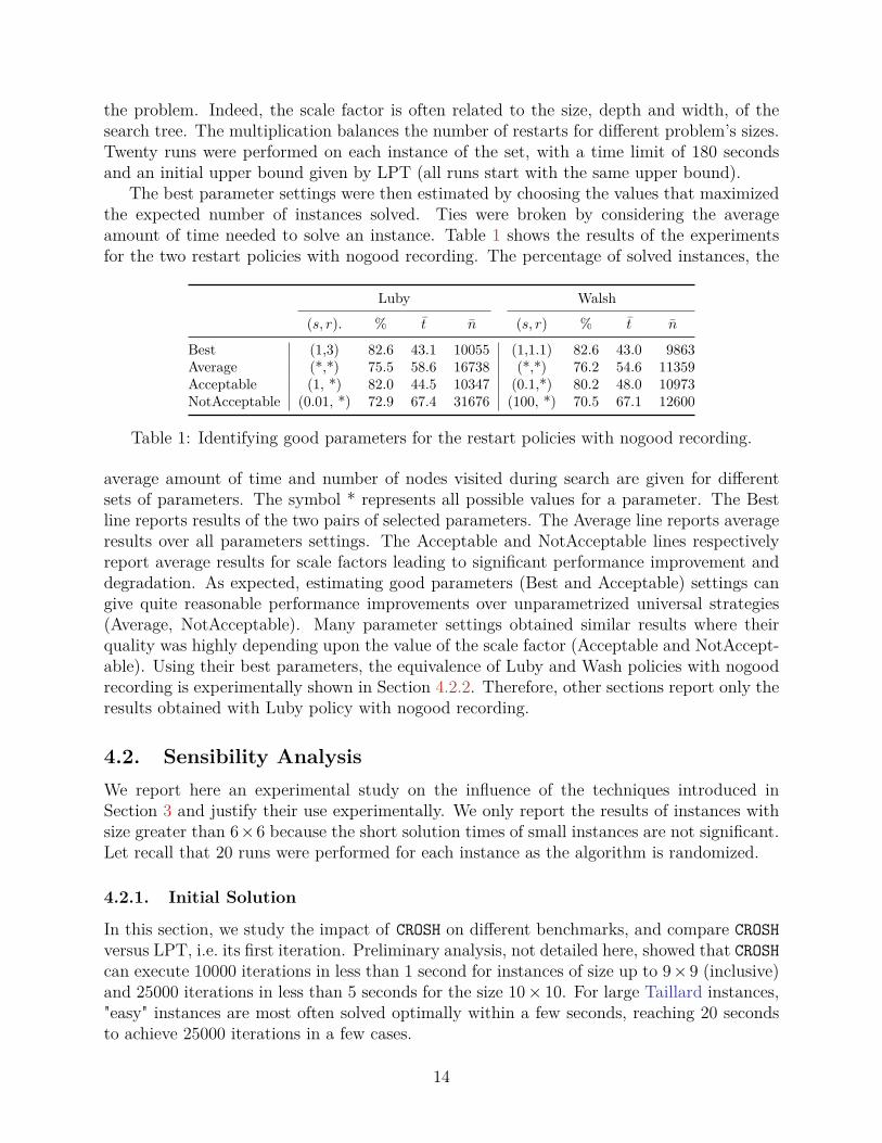
The best parameter settings were then estimated by choosing the values that maximizedthe expected number of instances solved. Ties were broken by considering the averageamount of time needed to solve an instance. Table 1 shows the results of the experimentsfor the two restart policies with nogood recording. The percentage of solved instances, the

Luby Walsh

(s, r). % t n (s, r) % t n

Best (1,3) 82.6 43.1 10055 (1,1.1) 82.6 43.0 9863Average (*,*) 75.5 58.6 16738 (*,*) 76.2 54.6 11359Acceptable (1, *) 82.0 44.5 10347 (0.1,*) 80.2 48.0 10973NotAcceptable (0.01, *) 72.9 67.4 31676 (100, *) 70.5 67.1 12600

Table 1: Identifying good parameters for the restart policies with nogood recording.

average amount of time and number of nodes visited during search are given for differentsets of parameters. The symbol * represents all possible values for a parameter. The Bestline reports results of the two pairs of selected parameters. The Average line reports averageresults over all parameters settings. The Acceptable and NotAcceptable lines respectivelyreport average results for scale factors leading to significant performance improvement anddegradation. As expected, estimating good parameters (Best and Acceptable) settings cangive quite reasonable performance improvements over unparametrized universal strategies(Average, NotAcceptable). Many parameter settings obtained similar results where theirquality was highly depending upon the value of the scale factor (Acceptable and NotAccept-able). Using their best parameters, the equivalence of Luby and Wash policies with nogoodrecording is experimentally shown in Section 4.2.2. Therefore, other sections report only theresults obtained with Luby policy with nogood recording.

4.2. Sensibility AnalysisWe report here an experimental study on the influence of the techniques introduced inSection 3 and justify their use experimentally. We only report the results of instances withsize greater than 6×6 because the short solution times of small instances are not significant.Let recall that 20 runs were performed for each instance as the algorithm is randomized.

4.2.1. Initial Solution

In this section, we study the impact of CROSH on different benchmarks, and compare CROSHversus LPT, i.e. its first iteration. Preliminary analysis, not detailed here, showed that CROSHcan execute 10000 iterations in less than 1 second for instances of size up to 9× 9 (inclusive)and 25000 iterations in less than 5 seconds for the size 10× 10. For large Taillard instances,"easy" instances are most often solved optimally within a few seconds, reaching 20 secondsto achieve 25000 iterations in a few cases.

14

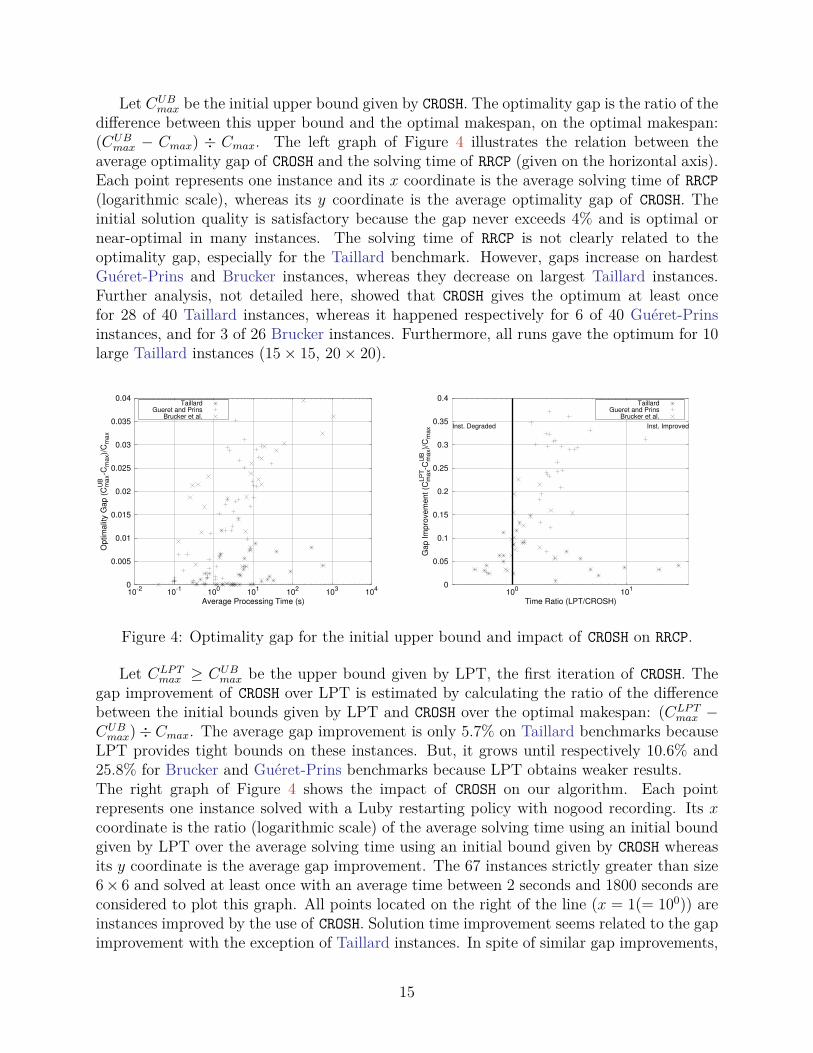
Let CUBmax be the initial upper bound given by CROSH. The optimality gap is the ratio of the

difference between this upper bound and the optimal makespan, on the optimal makespan:(CUB

max − Cmax) ÷ Cmax. The left graph of Figure 4 illustrates the relation between theaverage optimality gap of CROSH and the solving time of RRCP (given on the horizontal axis).Each point represents one instance and its x coordinate is the average solving time of RRCP(logarithmic scale), whereas its y coordinate is the average optimality gap of CROSH. Theinitial solution quality is satisfactory because the gap never exceeds 4% and is optimal ornear-optimal in many instances. The solving time of RRCP is not clearly related to theoptimality gap, especially for the Taillard benchmark. However, gaps increase on hardestGuéret-Prins and Brucker instances, whereas they decrease on largest Taillard instances.Further analysis, not detailed here, showed that CROSH gives the optimum at least oncefor 28 of 40 Taillard instances, whereas it happened respectively for 6 of 40 Guéret-Prinsinstances, and for 3 of 26 Brucker instances. Furthermore, all runs gave the optimum for 10large Taillard instances (15× 15, 20× 20).

0

0.005

0.01

0.015

0.02

0.025

0.03

0.035

0.04

10-2

10-1

100

101

102

103

104

Op

tim

alit

y G

ap

(C

UB

max-C

max)/

Cm

ax

Average Processing Time (s)

TaillardGueret and Prins

Brucker et al.

0

0.05

0.1

0.15

0.2

0.25

0.3

0.35

0.4

100

101

Ga

p I

mp

rove

me

nt

(Cm

ax

LP

T-C

UB

max)/

Cm

ax

Time Ratio (LPT/CROSH)

TaillardGueret and Prins

Brucker et al.

Inst. Degraded Inst. Improved

Figure 4: Optimality gap for the initial upper bound and impact of CROSH on RRCP.

Let CLPTmax ≥ CUB

max be the upper bound given by LPT, the first iteration of CROSH. Thegap improvement of CROSH over LPT is estimated by calculating the ratio of the differencebetween the initial bounds given by LPT and CROSH over the optimal makespan: (CLPT

max −CUBmax)÷ Cmax. The average gap improvement is only 5.7% on Taillard benchmarks because

LPT provides tight bounds on these instances. But, it grows until respectively 10.6% and25.8% for Brucker and Guéret-Prins benchmarks because LPT obtains weaker results.The right graph of Figure 4 shows the impact of CROSH on our algorithm. Each pointrepresents one instance solved with a Luby restarting policy with nogood recording. Its xcoordinate is the ratio (logarithmic scale) of the average solving time using an initial boundgiven by LPT over the average solving time using an initial bound given by CROSH whereasits y coordinate is the average gap improvement. The 67 instances strictly greater than size6× 6 and solved at least once with an average time between 2 seconds and 1800 seconds areconsidered to plot this graph. All points located on the right of the line (x = 1(= 100)) areinstances improved by the use of CROSH. Solution time improvement seems related to the gapimprovement with the exception of Taillard instances. In spite of similar gap improvements,

15

some Taillard instances are solved more than 10 times faster using CROSH whereas a fewinstances located on the left of (x = 1) are degraded.

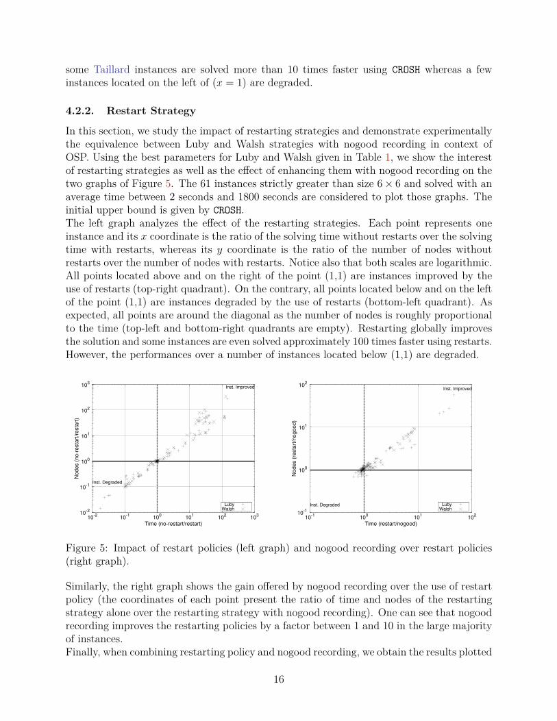
4.2.2. Restart Strategy

In this section, we study the impact of restarting strategies and demonstrate experimentallythe equivalence between Luby and Walsh strategies with nogood recording in context ofOSP. Using the best parameters for Luby and Walsh given in Table 1, we show the interestof restarting strategies as well as the effect of enhancing them with nogood recording on thetwo graphs of Figure 5. The 61 instances strictly greater than size 6× 6 and solved with anaverage time between 2 seconds and 1800 seconds are considered to plot those graphs. Theinitial upper bound is given by CROSH.The left graph analyzes the effect of the restarting strategies. Each point represents oneinstance and its x coordinate is the ratio of the solving time without restarts over the solvingtime with restarts, whereas its y coordinate is the ratio of the number of nodes withoutrestarts over the number of nodes with restarts. Notice also that both scales are logarithmic.All points located above and on the right of the point (1,1) are instances improved by theuse of restarts (top-right quadrant). On the contrary, all points located below and on the leftof the point (1,1) are instances degraded by the use of restarts (bottom-left quadrant). Asexpected, all points are around the diagonal as the number of nodes is roughly proportionalto the time (top-left and bottom-right quadrants are empty). Restarting globally improvesthe solution and some instances are even solved approximately 100 times faster using restarts.However, the performances over a number of instances located below (1,1) are degraded.

10-2

10-1

100

101

102

103

10-2

10-1

100

101

102

103

No

de

s (

no

-re

sta

rt/r

esta

rt)

Time (no-restart/restart)

LubyWalsh

Inst. Degraded

Inst. Improved

10-1

100

101

102

10-1

100

101

102

No

de

s (

resta

rt/n

og

oo

d)

Time (restart/nogood)

LubyWalsh

Inst. Degraded

Inst. Improved

Figure 5: Impact of restart policies (left graph) and nogood recording over restart policies(right graph).

Similarly, the right graph shows the gain offered by nogood recording over the use of restartpolicy (the coordinates of each point present the ratio of time and nodes of the restartingstrategy alone over the restarting strategy with nogood recording). One can see that nogoodrecording improves the restarting policies by a factor between 1 and 10 in the large majorityof instances.Finally, when combining restarting policy and nogood recording, we obtain the results plotted

16

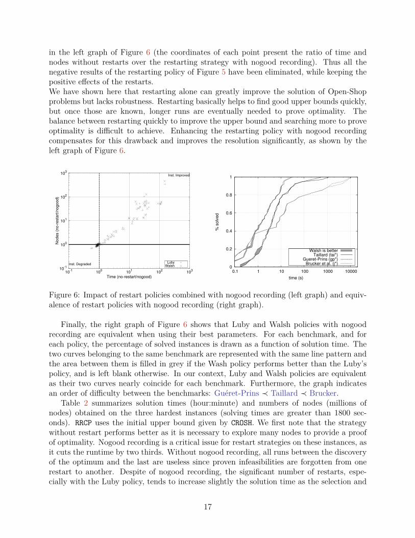
in the left graph of Figure 6 (the coordinates of each point present the ratio of time andnodes without restarts over the restarting strategy with nogood recording). Thus all thenegative results of the restarting policy of Figure 5 have been eliminated, while keeping thepositive effects of the restarts.We have shown here that restarting alone can greatly improve the solution of Open-Shopproblems but lacks robustness. Restarting basically helps to find good upper bounds quickly,but once those are known, longer runs are eventually needed to prove optimality. Thebalance between restarting quickly to improve the upper bound and searching more to proveoptimality is difficult to achieve. Enhancing the restarting policy with nogood recordingcompensates for this drawback and improves the resolution significantly, as shown by theleft graph of Figure 6.

10-1

100

101

102

103

10-1

100

101

102

103

No

de

s (

no

-re

sta

rt/n

og

oo

d)

Time (no-restart/nogood)

LubyWalsh

Inst. Degraded

Inst. Improved

0

0.2

0.4

0.6

0.8

1

0.1 1 10 100 1000 10000

% s

olv

ed

time (s)

Walsh is betterTaillard (tai*)

Gueret-Prins (gp*)Brucker et al. (j*)

Figure 6: Impact of restart policies combined with nogood recording (left graph) and equiv-alence of restart policies with nogood recording (right graph).

Finally, the right graph of Figure 6 shows that Luby and Walsh policies with nogoodrecording are equivalent when using their best parameters. For each benchmark, and foreach policy, the percentage of solved instances is drawn as a function of solution time. Thetwo curves belonging to the same benchmark are represented with the same line pattern andthe area between them is filled in grey if the Wash policy performs better than the Luby’spolicy, and is left blank otherwise. In our context, Luby and Walsh policies are equivalentas their two curves nearly coincide for each benchmark. Furthermore, the graph indicatesan order of difficulty between the benchmarks: Guéret-Prins ≺ Taillard ≺ Brucker.

Table 2 summarizes solution times (hour:minute) and numbers of nodes (millions ofnodes) obtained on the three hardest instances (solving times are greater than 1800 sec-onds). RRCP uses the initial upper bound given by CROSH. We first note that the strategywithout restart performs better as it is necessary to explore many nodes to provide a proofof optimality. Nogood recording is a critical issue for restart strategies on these instances, asit cuts the runtime by two thirds. Without nogood recording, all runs between the discoveryof the optimum and the last are useless since proven infeasibilities are forgotten from onerestart to another. Despite of nogood recording, the significant number of restarts, espe-cially with the Luby policy, tends to increase slightly the solution time as the selection and

17

propagation of initial choices are repeatedly performed. The Walsh strategy with nogoodrecording yields slightly better solution time than the Luby’s policy. However, its efficiencyheavily depends on nogood recording as it performs longer runs.

Restart Nogood Recording

Instance No Restart Luby Walsh Luby Walsh

Name Opt t n t n t n t n t n

j7-per0-0 1048 1:43 1.21 5:56 4.66 18:10 12.76 2:10 1.57 2:03 1.25j8-per0-1 1039 2:13 1.16 10:22 5.95 23:12 12.29 3:07 1.65 3:00 1.38j8-per10-2 1002 1:03 0.56 8:46 5.11 8:50 4.72 1:17 0.68 1:13 0.57

Table 2: The average solution time t (hour:minute) and number of nodes n (millions ofnodes) for the given alternatives applied to the three hardest instances.

4.2.3. Robustness

Lastly, we analyzed the robustness of RRCP for the Luby restart policy with nogood recordingand the initial upper bound given by CROSH. Robustness refers, in our case, to the sensitivityto the initial upper bound and to the randomized decision process, from one run of RRCP toanother. For each instance, we compute the ratio of the standard deviation on the averageruntime: std(t)÷ t. Then, we compute the average ratio for each benchmark. The Taillardbenchmark gives the highest average ratio equal to 62% because no optimality proof isneeded. Solution times largely differ according to the optimality of the initial upper boundfrom one execution to another. The instance is closed without branching if the initial boundis optimal, otherwise starting a complete search leads to an increase in solution time. Atthe contrary, our algorithm is more robust on Guéret-Prins and Brucker benchmarks withaverage ratios of 16% and 9%. Indeed, it spends more time to prove optimality than to reachan optimal solution because the proof requires the exploration of many nodes.

4.3. Comparison to Other ApproachesIn this section, we compare results of our algorithm without time limit, using the Lubyrestarting policy with nogood recording and the initial bound given by CROSH, to other ap-proaches. Tables 3, 4 and 5 summarize the results of different approaches on the Taillard,Brucker and Guéret-Prins benchmarks. The tables include the best results obtained by thegenetic algorithm (GA-Pri – Prins, 2000), the ant colony algorithm (ACO-Blu – Blum, 2005),the particle swarm algorithm (PSO-Sha – Sha and Hsu, 2008), the branch-and-bound withintelligent backtracking (BB-Gue – Guéret et al., 2000), the branch-and-bound with consis-tency tests (BB-Do – Dorndorf et al., 2001), and the transformation into SAT of (SAT-TaTamura et al., 2006). The papers cited above sometimes report several results obtained withvariants of their approach, and we have quoted the best of them in Tables 3, 4 and 5. Thecolumn Opt gives the optimal makespan for each instance. The value of a reported objectiveis in bold when it is equal to the optimal makespan.We report the objective value after a unique run of GA-Pri and do not report its solving

18

time. ACO-Blu and PSO-Sha results were obtained by 20 runs on each problem using PCswith AMD Athlon 1.1 GHz CPU running under Linux, and PCs with AMD Athlon 1.8 GHzrunning under Windows XP respectively. For each of these approaches, the average objectivevalue (Avg) and average solving time t are given. The best objective value (Best) is alsogiven when it is not equal to the optimal makespan for all instances. The best objectivevalue of PSO-Sha is marked with a † if the decoding operator is not hybridized with beamsearch.We report only the objective value of BB-Gue as it reached often the limit of 250 000 back-tracks (about 3 hours of CPU time on a Pentium PC clocked at 133 MHz).We report the solving time t of BB-Do, which has been tested on a Pentium II 333 MHzin an MSDOS environment with a time limit of 5 hours, since it identified many optimalsolutions. The symbol – indicates that the bottom-up algorithm was stopped before findinga solution, whereas the final upper bound is given in brackets when the top-down algorithmwas interrupted.Solution times of SAT-Ta using Intel Xeon 2.8GHz 4GB memory are reported with the ex-ception of the experiments on j7-per0-0 and j8-per0-1 problems which were done using10 Mac mini machines (PowerPC G4 1.42GHz 1GB memory) running in parallel and bydividing each problem into 120 subproblems. Optimal solutions were found and proven forboth instances within 13 hours (marked with M in Table 4).(CNR-Cha – Chatzikokolakis et al., 2004) interrupted their search after 120 minutes andonly if the time elapsed after the last improvement exceeded 30 minutes. CNR-Cha did notreport either solution times, or makespan.MCS-Lab applied their bottom-up algorithm with a time limit of 5 seconds for each sub-problem and ran experiments on a Dell Latitude D600 laptop, 1.4 GHz. If the time limitwas reached on a given subproblem, then the search was stopped without returning anysolution. MCS-Lab did not report solution times but it is possible to estimate an overallruntime for each instance. A bottom-up algorithm solves Cmax − CLB

max infeasible subprob-lems and a single feasible subproblem giving the optimum. The number of subproblemsdepends on each particular instance despite CLB

max is always equal to 1000 for Brucker andGuéret-Prins benchmarks. MCS-Lab reported that the early iterations were short and thatthe latter ones become longer during the transition phase. Therefore, our estimation ofits runtime, inspired by the dichotomous variant of bottom-up (see Section 1), is equal to5× dlog2

(Cmax − CLB

max + 1)

+ 1e seconds.As mentioned before, our experiments were realized on a cluster with Linux machines,

each node with 1 GB of RAM and a AMD 2.2 GHz processor. We report the average solvingtime t and number of nodes n of our approach over 20 runs. Note that the comparison of thesolving times might not be always significant because of the differences among computationalplatforms.

Results for the Taillard Instances (Table 3) This set of instances is considered easysince no optimality proof is needed, and it is thus solved efficiently by metaheuristics. Forexample, only six instances remained unsolved after a unique run of GA-Pri. ACO-Bluand PSO-Sha closed the remaining instances with good solution times even if some runson several instances led to suboptimal solutions. These failures are not clearly related tothe size of the problem. On the contrary, CNR-Cha obtained its weakest results on this

19

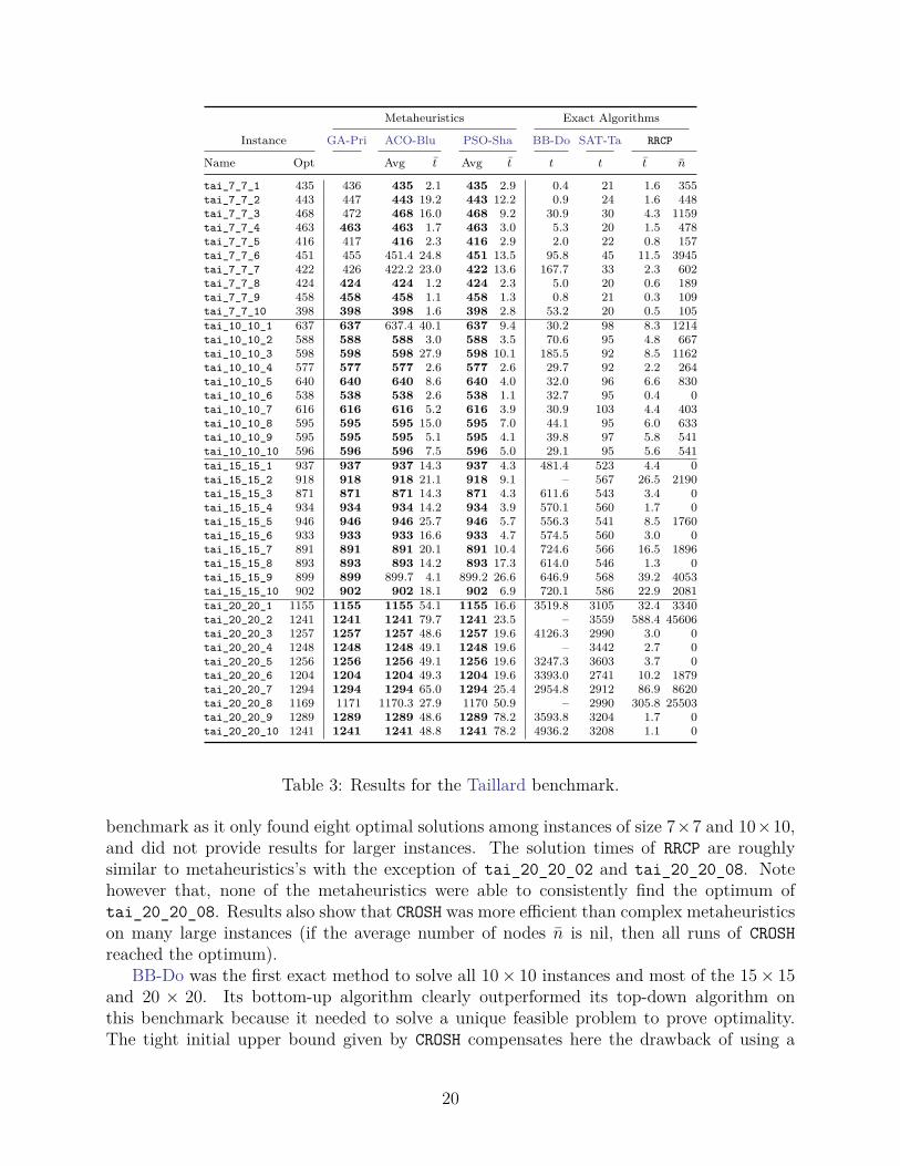
Metaheuristics Exact Algorithms

Instance GA-Pri ACO-Blu PSO-Sha BB-Do SAT-Ta RRCP

Name Opt Avg t Avg t t t t n

tai_7_7_1 435 436 435 2.1 435 2.9 0.4 21 1.6 355tai_7_7_2 443 447 443 19.2 443 12.2 0.9 24 1.6 448tai_7_7_3 468 472 468 16.0 468 9.2 30.9 30 4.3 1159tai_7_7_4 463 463 463 1.7 463 3.0 5.3 20 1.5 478tai_7_7_5 416 417 416 2.3 416 2.9 2.0 22 0.8 157tai_7_7_6 451 455 451.4 24.8 451 13.5 95.8 45 11.5 3945tai_7_7_7 422 426 422.2 23.0 422 13.6 167.7 33 2.3 602tai_7_7_8 424 424 424 1.2 424 2.3 5.0 20 0.6 189tai_7_7_9 458 458 458 1.1 458 1.3 0.8 21 0.3 109tai_7_7_10 398 398 398 1.6 398 2.8 53.2 20 0.5 105tai_10_10_1 637 637 637.4 40.1 637 9.4 30.2 98 8.3 1214tai_10_10_2 588 588 588 3.0 588 3.5 70.6 95 4.8 667tai_10_10_3 598 598 598 27.9 598 10.1 185.5 92 8.5 1162tai_10_10_4 577 577 577 2.6 577 2.6 29.7 92 2.2 264tai_10_10_5 640 640 640 8.6 640 4.0 32.0 96 6.6 830tai_10_10_6 538 538 538 2.6 538 1.1 32.7 95 0.4 0tai_10_10_7 616 616 616 5.2 616 3.9 30.9 103 4.4 403tai_10_10_8 595 595 595 15.0 595 7.0 44.1 95 6.0 633tai_10_10_9 595 595 595 5.1 595 4.1 39.8 97 5.8 541tai_10_10_10 596 596 596 7.5 596 5.0 29.1 95 5.6 541tai_15_15_1 937 937 937 14.3 937 4.3 481.4 523 4.4 0tai_15_15_2 918 918 918 21.1 918 9.1 – 567 26.5 2190tai_15_15_3 871 871 871 14.3 871 4.3 611.6 543 3.4 0tai_15_15_4 934 934 934 14.2 934 3.9 570.1 560 1.7 0tai_15_15_5 946 946 946 25.7 946 5.7 556.3 541 8.5 1760tai_15_15_6 933 933 933 16.6 933 4.7 574.5 560 3.0 0tai_15_15_7 891 891 891 20.1 891 10.4 724.6 566 16.5 1896tai_15_15_8 893 893 893 14.2 893 17.3 614.0 546 1.3 0tai_15_15_9 899 899 899.7 4.1 899.2 26.6 646.9 568 39.2 4053tai_15_15_10 902 902 902 18.1 902 6.9 720.1 586 22.9 2081tai_20_20_1 1155 1155 1155 54.1 1155 16.6 3519.8 3105 32.4 3340tai_20_20_2 1241 1241 1241 79.7 1241 23.5 – 3559 588.4 45606tai_20_20_3 1257 1257 1257 48.6 1257 19.6 4126.3 2990 3.0 0tai_20_20_4 1248 1248 1248 49.1 1248 19.6 – 3442 2.7 0tai_20_20_5 1256 1256 1256 49.1 1256 19.6 3247.3 3603 3.7 0tai_20_20_6 1204 1204 1204 49.3 1204 19.6 3393.0 2741 10.2 1879tai_20_20_7 1294 1294 1294 65.0 1294 25.4 2954.8 2912 86.9 8620tai_20_20_8 1169 1171 1170.3 27.9 1170 50.9 – 2990 305.8 25503tai_20_20_9 1289 1289 1289 48.6 1289 78.2 3593.8 3204 1.7 0tai_20_20_10 1241 1241 1241 48.8 1241 78.2 4936.2 3208 1.1 0

Table 3: Results for the Taillard benchmark.

benchmark as it only found eight optimal solutions among instances of size 7×7 and 10×10,and did not provide results for larger instances. The solution times of RRCP are roughlysimilar to metaheuristics’s with the exception of tai_20_20_02 and tai_20_20_08. Notehowever that, none of the metaheuristics were able to consistently find the optimum oftai_20_20_08. Results also show that CROSH was more efficient than complex metaheuristicson many large instances (if the average number of nodes n is nil, then all runs of CROSHreached the optimum).

BB-Do was the first exact method to solve all 10× 10 instances and most of the 15× 15and 20 × 20. Its bottom-up algorithm clearly outperformed its top-down algorithm onthis benchmark because it needed to solve a unique feasible problem to prove optimality.The tight initial upper bound given by CROSH compensates here the drawback of using a

20

top-down algorithm. Furthermore, the diversification provided by the randomization andrestart mechanism helps to escape from bad initial choices whereas some instances remainedunsolved by BB-Do such as tai_15_15_02. With equivalent computational platforms, RRCPclearly outperforms SAT-Ta, the first exact method to close the benchmark. However, thetotal CPU time of SAT-Ta linearly fits with the number of clauses on this benchmark,whereas it is not necessarily the case with our algorithm. For example, tai_20_20_08 is notmore difficult than others 20× 20 as opposed to other approaches. Last, MCS-Lab did notreport results on this benchmark.

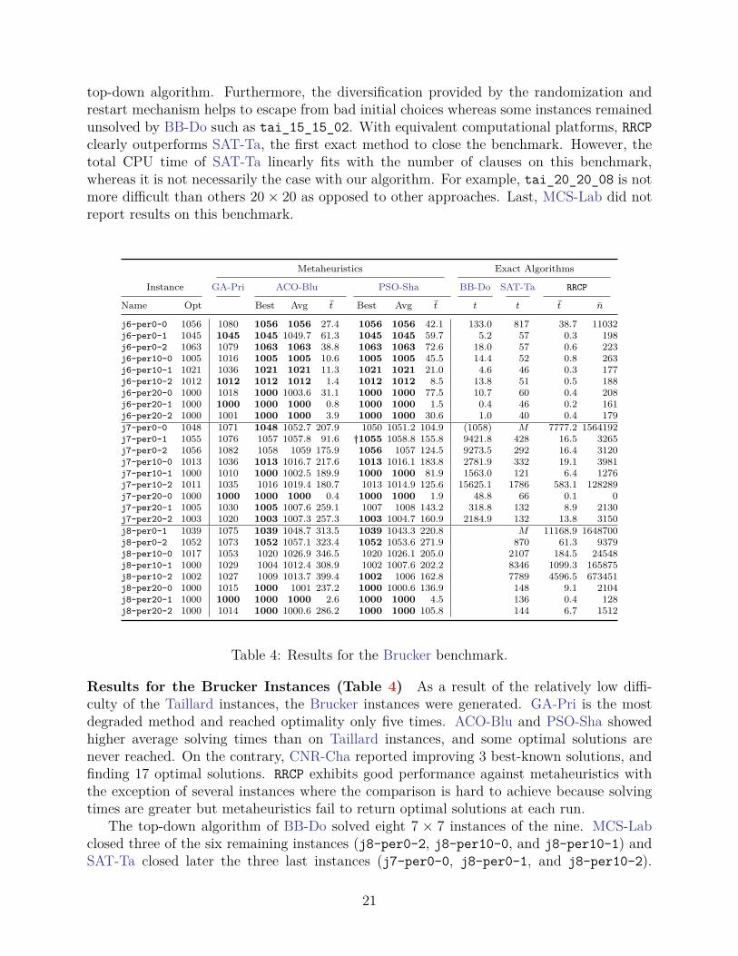
Metaheuristics Exact Algorithms

Instance GA-Pri ACO-Blu PSO-Sha BB-Do SAT-Ta RRCP

Name Opt Best Avg t Best Avg t t t t n

j6-per0-0 1056 1080 1056 1056 27.4 1056 1056 42.1 133.0 817 38.7 11032j6-per0-1 1045 1045 1045 1049.7 61.3 1045 1045 59.7 5.2 57 0.3 198j6-per0-2 1063 1079 1063 1063 38.8 1063 1063 72.6 18.0 57 0.6 223j6-per10-0 1005 1016 1005 1005 10.6 1005 1005 45.5 14.4 52 0.8 263j6-per10-1 1021 1036 1021 1021 11.3 1021 1021 21.0 4.6 46 0.3 177j6-per10-2 1012 1012 1012 1012 1.4 1012 1012 8.5 13.8 51 0.5 188j6-per20-0 1000 1018 1000 1003.6 31.1 1000 1000 77.5 10.7 60 0.4 208j6-per20-1 1000 1000 1000 1000 0.8 1000 1000 1.5 0.4 46 0.2 161j6-per20-2 1000 1001 1000 1000 3.9 1000 1000 30.6 1.0 40 0.4 179j7-per0-0 1048 1071 1048 1052.7 207.9 1050 1051.2 104.9 (1058) M 7777.2 1564192j7-per0-1 1055 1076 1057 1057.8 91.6 †1055 1058.8 155.8 9421.8 428 16.5 3265j7-per0-2 1056 1082 1058 1059 175.9 1056 1057 124.5 9273.5 292 16.4 3120j7-per10-0 1013 1036 1013 1016.7 217.6 1013 1016.1 183.8 2781.9 332 19.1 3981j7-per10-1 1000 1010 1000 1002.5 189.9 1000 1000 81.9 1563.0 121 6.4 1276j7-per10-2 1011 1035 1016 1019.4 180.7 1013 1014.9 125.6 15625.1 1786 583.1 128289j7-per20-0 1000 1000 1000 1000 0.4 1000 1000 1.9 48.8 66 0.1 0j7-per20-1 1005 1030 1005 1007.6 259.1 1007 1008 143.2 318.8 132 8.9 2130j7-per20-2 1003 1020 1003 1007.3 257.3 1003 1004.7 160.9 2184.9 132 13.8 3150j8-per0-1 1039 1075 1039 1048.7 313.5 1039 1043.3 220.8 M 11168.9 1648700j8-per0-2 1052 1073 1052 1057.1 323.4 1052 1053.6 271.9 870 61.3 9379j8-per10-0 1017 1053 1020 1026.9 346.5 1020 1026.1 205.0 2107 184.5 24548j8-per10-1 1000 1029 1004 1012.4 308.9 1002 1007.6 202.2 8346 1099.3 165875j8-per10-2 1002 1027 1009 1013.7 399.4 1002 1006 162.8 7789 4596.5 673451j8-per20-0 1000 1015 1000 1001 237.2 1000 1000.6 136.9 148 9.1 2104j8-per20-1 1000 1000 1000 1000 2.6 1000 1000 4.5 136 0.4 128j8-per20-2 1000 1014 1000 1000.6 286.2 1000 1000 105.8 144 6.7 1512

Table 4: Results for the Brucker benchmark.

Results for the Brucker Instances (Table 4) As a result of the relatively low diffi-culty of the Taillard instances, the Brucker instances were generated. GA-Pri is the mostdegraded method and reached optimality only five times. ACO-Blu and PSO-Sha showedhigher average solving times than on Taillard instances, and some optimal solutions arenever reached. On the contrary, CNR-Cha reported improving 3 best-known solutions, andfinding 17 optimal solutions. RRCP exhibits good performance against metaheuristics withthe exception of several instances where the comparison is hard to achieve because solvingtimes are greater but metaheuristics fail to return optimal solutions at each run.

The top-down algorithm of BB-Do solved eight 7 × 7 instances of the nine. MCS-Labclosed three of the six remaining instances (j8-per0-2, j8-per10-0, and j8-per10-1) andSAT-Ta closed later the three last instances (j7-per0-0, j8-per0-1, and j8-per10-2).

21

With the exception of j7-per10-2, j8-per10-0 and j8-per10-1, RRCP yields solving timesbelow or similar to estimated runtimes of MCS-Lab which range from 5 to 35 seconds.Solving times of SAT-Ta stay greater than RRCP’s, especially for j7-per0-0 and j8-per0-1where their experiments required great computation time. On this benchmark, their solvingtimes do not exhibit a linear behaviour on the problem’s size.

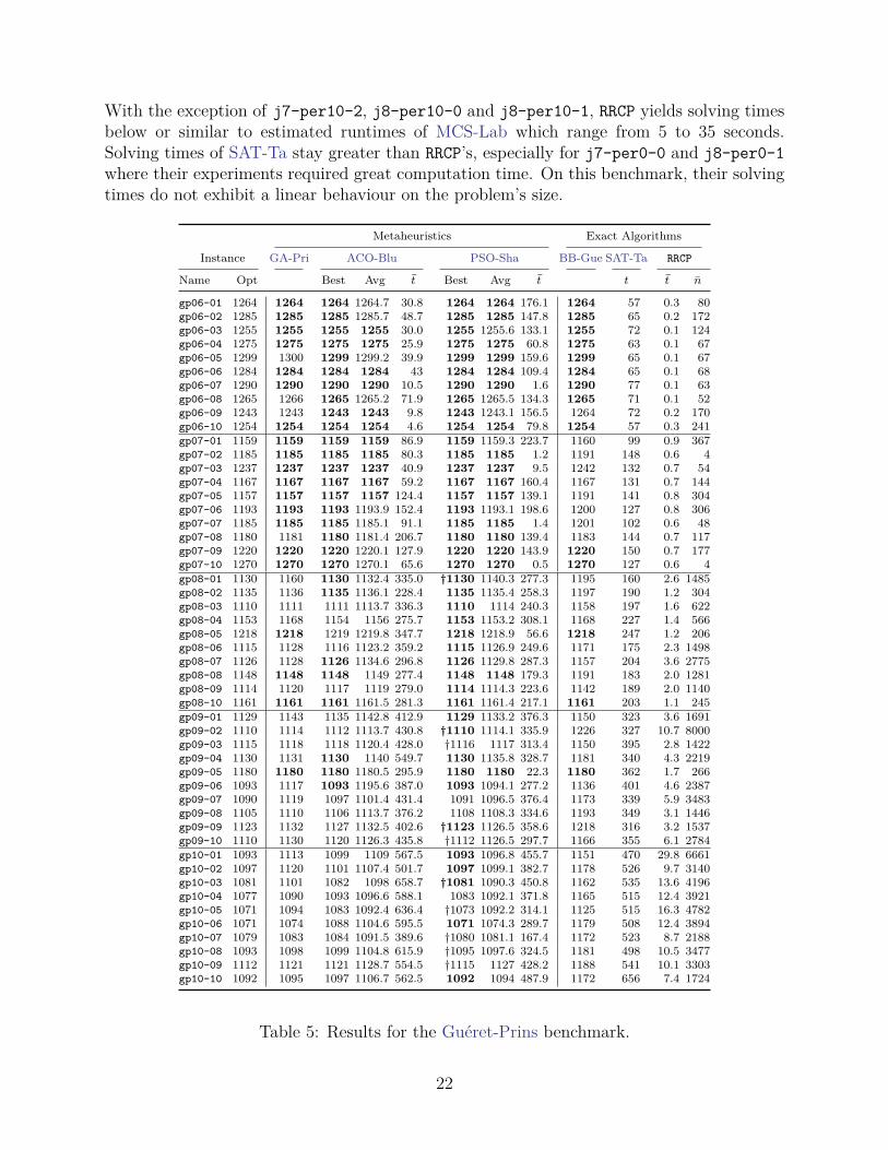
Metaheuristics Exact Algorithms

Instance GA-Pri ACO-Blu PSO-Sha BB-Gue SAT-Ta RRCP

Name Opt Best Avg t Best Avg t t t n

gp06-01 1264 1264 1264 1264.7 30.8 1264 1264 176.1 1264 57 0.3 80gp06-02 1285 1285 1285 1285.7 48.7 1285 1285 147.8 1285 65 0.2 172gp06-03 1255 1255 1255 1255 30.0 1255 1255.6 133.1 1255 72 0.1 124gp06-04 1275 1275 1275 1275 25.9 1275 1275 60.8 1275 63 0.1 67gp06-05 1299 1300 1299 1299.2 39.9 1299 1299 159.6 1299 65 0.1 67gp06-06 1284 1284 1284 1284 43 1284 1284 109.4 1284 65 0.1 68gp06-07 1290 1290 1290 1290 10.5 1290 1290 1.6 1290 77 0.1 63gp06-08 1265 1266 1265 1265.2 71.9 1265 1265.5 134.3 1265 71 0.1 52gp06-09 1243 1243 1243 1243 9.8 1243 1243.1 156.5 1264 72 0.2 170gp06-10 1254 1254 1254 1254 4.6 1254 1254 79.8 1254 57 0.3 241gp07-01 1159 1159 1159 1159 86.9 1159 1159.3 223.7 1160 99 0.9 367gp07-02 1185 1185 1185 1185 80.3 1185 1185 1.2 1191 148 0.6 4gp07-03 1237 1237 1237 1237 40.9 1237 1237 9.5 1242 132 0.7 54gp07-04 1167 1167 1167 1167 59.2 1167 1167 160.4 1167 131 0.7 144gp07-05 1157 1157 1157 1157 124.4 1157 1157 139.1 1191 141 0.8 304gp07-06 1193 1193 1193 1193.9 152.4 1193 1193.1 198.6 1200 127 0.8 306gp07-07 1185 1185 1185 1185.1 91.1 1185 1185 1.4 1201 102 0.6 48gp07-08 1180 1181 1180 1181.4 206.7 1180 1180 139.4 1183 144 0.7 117gp07-09 1220 1220 1220 1220.1 127.9 1220 1220 143.9 1220 150 0.7 177gp07-10 1270 1270 1270 1270.1 65.6 1270 1270 0.5 1270 127 0.6 4gp08-01 1130 1160 1130 1132.4 335.0 †1130 1140.3 277.3 1195 160 2.6 1485gp08-02 1135 1136 1135 1136.1 228.4 1135 1135.4 258.3 1197 190 1.2 304gp08-03 1110 1111 1111 1113.7 336.3 1110 1114 240.3 1158 197 1.6 622gp08-04 1153 1168 1154 1156 275.7 1153 1153.2 308.1 1168 227 1.4 566gp08-05 1218 1218 1219 1219.8 347.7 1218 1218.9 56.6 1218 247 1.2 206gp08-06 1115 1128 1116 1123.2 359.2 1115 1126.9 249.6 1171 175 2.3 1498gp08-07 1126 1128 1126 1134.6 296.8 1126 1129.8 287.3 1157 204 3.6 2775gp08-08 1148 1148 1148 1149 277.4 1148 1148 179.3 1191 183 2.0 1281gp08-09 1114 1120 1117 1119 279.0 1114 1114.3 223.6 1142 189 2.0 1140gp08-10 1161 1161 1161 1161.5 281.3 1161 1161.4 217.1 1161 203 1.1 245gp09-01 1129 1143 1135 1142.8 412.9 1129 1133.2 376.3 1150 323 3.6 1691gp09-02 1110 1114 1112 1113.7 430.8 †1110 1114.1 335.9 1226 327 10.7 8000gp09-03 1115 1118 1118 1120.4 428.0 †1116 1117 313.4 1150 395 2.8 1422gp09-04 1130 1131 1130 1140 549.7 1130 1135.8 328.7 1181 340 4.3 2219gp09-05 1180 1180 1180 1180.5 295.9 1180 1180 22.3 1180 362 1.7 266gp09-06 1093 1117 1093 1195.6 387.0 1093 1094.1 277.2 1136 401 4.6 2387gp09-07 1090 1119 1097 1101.4 431.4 1091 1096.5 376.4 1173 339 5.9 3483gp09-08 1105 1110 1106 1113.7 376.2 1108 1108.3 334.6 1193 349 3.1 1446gp09-09 1123 1132 1127 1132.5 402.6 †1123 1126.5 358.6 1218 316 3.2 1537gp09-10 1110 1130 1120 1126.3 435.8 †1112 1126.5 297.7 1166 355 6.1 2784gp10-01 1093 1113 1099 1109 567.5 1093 1096.8 455.7 1151 470 29.8 6661gp10-02 1097 1120 1101 1107.4 501.7 1097 1099.1 382.7 1178 526 9.7 3140gp10-03 1081 1101 1082 1098 658.7 †1081 1090.3 450.8 1162 535 13.6 4196gp10-04 1077 1090 1093 1096.6 588.1 1083 1092.1 371.8 1165 515 12.4 3921gp10-05 1071 1094 1083 1092.4 636.4 †1073 1092.2 314.1 1125 515 16.3 4782gp10-06 1071 1074 1088 1104.6 595.5 1071 1074.3 289.7 1179 508 12.4 3894gp10-07 1079 1083 1084 1091.5 389.6 †1080 1081.1 167.4 1172 523 8.7 2188gp10-08 1093 1098 1099 1104.8 615.9 †1095 1097.6 324.5 1181 498 10.5 3477gp10-09 1112 1121 1121 1128.7 554.5 †1115 1127 428.2 1188 541 10.1 3303gp10-10 1092 1095 1097 1106.7 562.5 1092 1094 487.9 1172 656 7.4 1724

Table 5: Results for the Guéret-Prins benchmark.

22

Results for the Guéret-Prins Instances (Table 5) The Guéret-Prins instances seemsto be more difficult to solve because the metaheuristics are less effective. Average results ofACO-Blu and PSO-Sha decrease according to problem size. In spite of higher solving times,fewer optimums are reached, especially with ACO-Blu. By comparison, GA-Pri is moreeffective than with Brucker benchmark and CNR-Cha claims to improve 12 solutions. RRCPis particularly well-suited for this series of problems and it prevails over all metaheuristicsin every problem size.

BB-Gue solved most instances to optimality up to size 6 × 6 as well as a few largeinstances. BB-Do did not report results on this benchmark and MCS-Lab reported closingall the instances, but again did not report detailed solution times. Solving times of RRCPare always lower than estimated runtimes of MCS-Lab which range from 40 to 50 seconds.Solving times of SAT-Ta decrease and again linearly fit the number of clauses, but do notcompete with RRCP’s.

5. ConclusionWe have presented a constraint programming algorithm to solve the Open-Shop problem.This algorithm consists of computing an initial upper bound before solving a high-leveldeclarative model (tasks, resources, precedences) by a top-down branch-and-bound enhancedwith randomization and restart.The computational results matched the metaheuristics for the Taillard benchmark, whereaswe obtained better solution quality with solution times that are orders of magnitude lowerthan the metaheuristics for the Brucker and Guéret-Prins benchmarks. The computationalresults also outperformed all exact approaches that reported detailed solution times.In further research, we will apply other branching schemes. In addition, subsequent researchtopics include the study of other shop problems such as Flow-Shop Problems and Job-ShopProblems.

ReferencesBaptiste, Philippe, Claude Le Pape. 1996. Edge-finding constraint propagation algorithmsfor disjunctive and cumulative scheduling. Proceedings of the Fifteenth Workshop of theU.K. Planning Special Interest Group.

Beck, J. Christopher, Andrew J. Davenport, Edward M. Sitarski, Mark S. Fox. 1997. Texture-based heuristics for scheduling revisited. AAAI/IAAI . 241–248.

Blum, Christian. 2005. Beam-ACO: hybridizing ant colony optimization with beam search:an application to open shop scheduling. Comput. Oper. Res. 32 1565–1591.

Bräsel, H., T. Tautenhahn, F. Werner. 1993. Constructive heuristic algorithms for the openshop problem. Computing 51 95–110.

Brucker, P., T. Hilbig, J. Hurink. 1996. A branch and bound algorithm for schedulingproblems with positive and negative time-lags. Tech. rep., Osnabrueck University.

23

Brucker, Peter, Andreas Drexl, Rolf Mohring, Klaus Neumann, Erwin Pesch. 1999. Resource-constrained project scheduling: Notation, classification, models, and methods. EuropeanJournal of Operational Research 112 3–41.

Brucker, Peter, Johann Hurink, Bernd Jurisch, Birgit Wöstmann. 1997. A branch & boundalgorithm for the open-shop problem. GO-II Meeting: Proceedings of the second interna-tional colloquium on Graphs and optimization. Elsevier Science Publishers B. V., Amster-dam, The Netherlands, 43–59.

Carlier, J., E. Pinson. 1994. Adjustment of heads and tails for the job-shop problem. Euro-pean Journal of Operational Research 78 146–161.

Caseau, Y., F. Laburthe. 1995. Disjunctive scheduling with task intervals. Tech. rep.,Laboratoire d’Informatique de I’Ecole Normale Superieure.

Cesta, A., A. Oddi. 1996. Gaining efficiency and flexibility in the simple temporal problem.TIME ’96: Proceedings of the 3rd Workshop on Temporal Representation and Reasoning(TIME’96). IEEE Computer Society, Washington, DC, USA, 45.

Chatzikokolakis, Konstantinos, George Boukeas, Panagiotis Stamatopoulos. 2004. Construc-tion and repair: A hybrid approach to search in csps. SETN 3025 2004.

Choco team. 2008. Choco: an open source java constraint programming library. URLhttp://choco.emn.fr.

Dechter, Rina. 2003. Temporal constraint networks. Constraint Processing. Morgan Kauf-mann, San Francisco, 333–362.

Dorndorf, U., E. Pesch, T. Phan Huy. 2001. Solving the open shop scheduling problem.Journal of Scheduling 4 157–174.

Frigioni, Daniele, Tobias Miller, Umberto Nanni, Christos D. Zaroliagis. 2001. An experi-mental study of dynamic algorithms for transitive closure. ACM Journal of ExperimentalAlgorithms 6 9.

Gondran, M., M. Minoux. 1984. Graphs and Algorithms. John Wiley & Sons, New York.

Gonzalez, T., S. Sahni. 1976. Open shop scheduling to minimize finish time. Journal of theAssociation for Computing Machinery 23 665–679.

Guéret, C., C. Prins. 1999. A new lower bound for the open shop problem. Annals ofOperations Research 92 165–183.

Guéret, Christelle. 1997. Problèmes d’ordonnancement sans contraintes de précédence.Thèse, Université de Technologie de Compiègne. Codirecteurs : C. Prins et J. Carlier.

Guéret, Christelle, Narendra Jussien, Christian Prins. 2000. Using intelligent backtrackingto improve branch-and-bound methods: An application to open-shop problems. EuropeanJournal of Operational Research 127 344–354.

24

Guéret, Christelle, Christian Prins. 1998. Forbidden intervals for open-shop problems. Tech.rep., École des Mines de Nantes.

Kellerer, H., U. Pferschy, D. Pisinger. 2004. Knapsack Problems. Springer, Berlin, Germany.

Kolisch, Rainer. 1996. Serial and parallel resource-constrained project scheduling methodsrevisited: Theory and computation. European Journal of Operational Research 90 320–333.

Laborie, Philippe. 2005. Complete mcs-based search: Application to resource constrainedproject scheduling. Leslie Pack Kaelbling, Alessandro Saffiotti, eds., IJCAI . ProfessionalBook Center, 181–186.

Le Pape, Claude, Philippe Couronne, Didier Vergamini, Vincent Gosselin. 1994. Time-versus-capacity compromises in project scheduling. Proceedings of the Thirteenth Workshopof the U.K. Planning Special Interest Group.

Lecoutre, Christophe, Lakhdar Sais, Sébastien Tabary, Vincent Vidal. 2007. Nogood record-ing from restarts. Manuela M. Veloso, ed., IJCAI 2007, Proceedings of the 20th Interna-tional Joint Conference on Artificial Intelligence, Hyderabad, India, January 6-12, 2007 .131–136.

Luby, Sinclair, Zuckerman. 1993. Optimal speedup of las vegas algorithms. IPL: InformationProcessing Letters 47 173–180.

Pearce, David J., Paul H. J. Kelly. 2006. A dynamic topological sort algorithm for directedacyclic graphs. ACM Journal of Experimental Algorithms 11 1–7.

Prins, Christian. 2000. Competitive genetic algorithms for the open-shop scheduling problem.Mathematical methods of operations research 52 389–411.

Sha, D. Y., Cheng-Yu Hsu. 2008. A new particle swarm optimization for the open shopscheduling problem. Comput. Oper. Res. 35 3243–3261.

Taillard, E. 1993. Benchmarks for basic scheduling problems. European Journal of OperationsResearch 64 278–285.

Tamura, Naoyuki, Akiko Taga, Satoshi Kitagawa, Mutsunori Banbara. 2006. Compilingfinite linear CSP into SAT. Principles and Practice of Constraint Programming - CP2006 , Lecture Notes in Computer Science, vol. 4204. Springer Berlin / Heidelberg, 590–603.

Vilím, Petr. 2004. O(n log n) filtering algorithms for unary resource constraint. CPAIOR2004, Nice, France, April 20-22, 2004 , Lecture Notes in Computer Science, vol. 3011.Springer, 335–347.

Walsh, Toby. 1999. Search in a small world. IJCAI ’99: Proceedings of the Sixteenth Inter-national Joint Conference on Artificial Intelligence. Morgan Kaufmann Publishers Inc.,San Francisco, CA, USA, 1172–1177.

25

Wu, Huayue, Peter van Beek. 2007. On universal restart strategies for backtracking search.Principles and Practice of Constraint Programming CP 2007 , Lecture Notes in ComputerScience, vol. 4741/2007. Springer Berlin / Heidelberg, 681–695.

26