ANL/ALCF-17/8

An Operator-Integration-Factor Splitting (OIFS) method for Incompressible Flows in Moving Domains

Argonne Leadership Computing Facility

About Argonne National Laboratory Argonne is a U.S. Department of Energy laboratory managed by UChicago Argonne, LLC under contract DE-AC02-06CH11357. The Laboratory’s main facility is outside Chicago, at 9700 South Cass Avenue, Argonne, Illinois 60439. For information about Argonne and its pioneering science and technology programs, see www.anl.gov.

DOCUMENT AVAILABILITY

Online Access: U.S. Department of Energy (DOE) reports produced after 1991 and a growing number of pre-1991 documents are available free via DOE’s SciTech Connect (http://www.osti.gov/scitech/)

Reports not in digital format may be purchased by the public from the National Technical Information Service (NTIS):

U.S. Department of Commerce National Technical Information Service 5301 Shawnee Rd Alexandria, VA 22312 www.ntis.gov Phone: (800) 553-NTIS (6847) or (703) 605-6000 Fax: (703) 605-6900 Email: orders@ntis.gov

Reports not in digital format are available to DOE and DOE contractors from the Office of Scientific and Technical Information (OSTI):

U.S. Department of Energy Office of Scientific and Technical Information P.O. Box 62 Oak Ridge, TN 37831-0062 www.osti.gov Phone: (865) 576-8401 Fax: (865) 576-5728 Email: reports@osti.gov

Disclaimer This report was prepared as an account of work sponsored by an agency of the United States Government. Neither the United States Government nor any agency thereof, nor UChicago Argonne, LLC, nor any of their employees or officers, makes any warranty, express or implied, or assumes any legal liability or responsibility for the accuracy, completeness, or usefulness of any information, apparatus, product, or process disclosed, or represents that its use would not infringe privately owned rights. Reference herein to any specific commercial product, process, or service by trade name, trademark, manufacturer, or otherwise, does not necessarily constitute or imply its endorsement, recommendation, or favoring by the United States Government or any agency thereof. The views and opinions of document authors expressed herein do not necessarily state or reflect those of the United States Government or any agency thereof, Argonne National Laboratory, or UChicago Argonne, LLC.

ANL/ALCF-17/8

An Operator-Integration-Factor Splitting (OIFS) method for Incompressible Flows in Moving Domains

prepared by Saumil S. Patel1, Paul F. Fischer2,3, Misun Min2, and Ananias G. Tomboulides2,4 1Argonne Leadership Computing Facility, Argonne National Laboratory 2Mathematics and Computer Science Division, Argonne National Laboratory 3Department of Mechanical Science and Engineering and Department of Computer Science, University of Illinois at Urbana-Champaign 4Aristotle University of Thessaloniki, Greece October 21, 2017

Contents

0.1 Introduction . . . . . . . . . . . . . . . . . . . . . . . . . . . . . . . . . . . . . . . . . . . . . . 1

0.2 Characteristic-Based Formulation for the Incompressible Navier-Stokes Equations . . . . . . . 2

0.2.1 Characteristic Formulation on a Static Domain . . . . . . . . . . . . . . . . . . . . . . 3

0.2.2 Characteristic/OIFS Formulation on a Moving Domain . . . . . . . . . . . . . . . . . 6

0.2.3 Runge-Kutta Time Integration on a Moving Domain . . . . . . . . . . . . . . . . . . . 8

0.2.4 Extension to the Navier-Stokes equation . . . . . . . . . . . . . . . . . . . . . . . . . . 9

0.3 Spectral Element Method . . . . . . . . . . . . . . . . . . . . . . . . . . . . . . . . . . . . . . 10

0.4 Computational Results . . . . . . . . . . . . . . . . . . . . . . . . . . . . . . . . . . . . . . . . 14

0.4.1 Temporal-Spatial Accuracy . . . . . . . . . . . . . . . . . . . . . . . . . . . . . . . . . 15

0.4.2 Flow in a Channel with a Moving Indentation . . . . . . . . . . . . . . . . . . . . . . . 15

0.4.3 Peristaltic Pumping . . . . . . . . . . . . . . . . . . . . . . . . . . . . . . . . . . . . . 20

0.4.4 TCC-III Engine . . . . . . . . . . . . . . . . . . . . . . . . . . . . . . . . . . . . . . . . 22

0.4.5 TCC-III Engine: Computational Performance . . . . . . . . . . . . . . . . . . . . . . . 23

0.4.6 A Pinched Pipe . . . . . . . . . . . . . . . . . . . . . . . . . . . . . . . . . . . . . . . . 24

0.5 Appendix . . . . . . . . . . . . . . . . . . . . . . . . . . . . . . . . . . . . . . . . . . . . . . . 25

0.5.1 Outflow Boundary Condition . . . . . . . . . . . . . . . . . . . . . . . . . . . . . . . . 25

0.5.2 Material Derivative of the Jacobian . . . . . . . . . . . . . . . . . . . . . . . . . . . . . 27

0.6 Conclusions . . . . . . . . . . . . . . . . . . . . . . . . . . . . . . . . . . . . . . . . . . . . . . 27

2

Abstract

In this paper, we present a characteristic-based numerical procedure for simulating incompressible flows indomains with moving boundaries. Our approach utilizes an operator-integration-factor splitting techniqueto help produce an efficient and stable numerical scheme. Using the spectral element method and anarbitrary Lagrangian-Eulerian formulation, we investigate flows where the convective acceleration effects arenon-negligible. Several examples, ranging from laminar to turbulent flows, are considered. Comparisons witha standard, semi-implicit time-stepping procedure illustrate the improved performance of the scheme.

0.1 Introduction

Predicting the motion of a fluid in a domain with moving boundaries has been one of the major challenges incomputational physics. Specific examples of moving boundary problems include free-surface flows, flows inblood vessels, and in-cylinder flows within internal combustion (IC) engines. A variety of numerical algorithmshave been proposed to tackle such problems. Most techniques incorporate a Lagrangian description of theboundary [1, 2, 3]. Such schemes may be considered to be in the class of arbitrary Lagrangian-Eulerian (ALE)methods [4], where the entire mesh is updated, perhaps at every timestep, in order to conform to the newboundary while the flow field is solved using an Eulerian approach.

The main feature of moving domain problems is the unsteadiness of the flow field. This feature isapparent in IC engines where multiple mechanisms generate turbulent flow fields [5]. Turbulence in IC enginespresents a challenge for computational fluid dynamic (CFD) algorithms, due primarily to the broad range oflength and time scales that need to be resolved. Specifically, simulations need to predict the evolution of avariety of flow structures (boundary layers, eddys, vortices, etc.) in the vicinity of complex domains that aremoving. Executing these simulations accurately and in a reasonable amount of time can ultimately lead toengine design concepts with improved efficiency.

Advances in high-performance parallel computers, scalable iterative solvers, and high-order discretizationshave led to much progress toward direct numerical simulation (DNS) and large eddy simulation (LES) ofturbulent flows in IC engines. LES has become a popular method of choice to study turbulence in ICengines [6, 7]. Due to the use of subgrid scale models, LES allows for a lower grid resolution while beingable to represent more flow structure (eddies and vortices) than a traditional Reynolds Averaged NavierStokes (RANS) approach. Progress and reviews of LES models for IC engines can be found in [8]. DNScalculations have also been performed with spectral element methods (SEM), making significant advances inthe investigations of cycle-to-cycle flow-field variations [9] and wall heat transfer [10] under engine-relevantconditions.

Since its introduction by Patera [11], several developments have made the spectral element method apowerful tool for the simulation of turbulence in complex geometries. Key advances include ALE formulationsbased on the lPN − lPN−2 spectral element method for incompressible and low-Mach number flows [10, 12, 13,14, 15]; stable fluid-structure interaction (FSI) solution strategies[15]; high-order operator splitting strategiesthat lead to decoupled linear symmetric positive-definite subproblems at each timestep [16, 17, 18, 19, 20];fast multilevel preconditioners [21, 22, 23] coupled with scalable parallel coarse grid solvers [24, 25, 26]; stableformulations for the convective operator [27, 28, 29]; and high-performance implementations [30].

The focus of this work is to build upon the current state of ALE formulations by incorporating atime-integration scheme that can solve the incompressible Navier-Stokes equations faster than standardtechniques. Using the lPN − lPN spectral element method [15, 31], we develop a scheme whose aim is toresolve turbulent flows with prescribed boundary motion. The specific application is for the flow generateddue to piston and intake valve motion in IC engines.

The performance of the engine relies heavily on how well turbulence can promote large and small-scalemixing between the fuel and air prior to combustion [5]. Indeed, Schiffman et.al [7] have indicated that theearly phase of the intake “jet” flow in an IC engine is critical to the evolution of the flow within a combustionchamber (or cylinder). Their results indicate that flow through the small intake valve region required refinedgrids for accuracy. This requirement came at a substantial computational cost, resulting in simulations thatran for three times longer than less-resolved grids [7].

The standard approach to efficient simulation of turbulent flow is to treat the nonlinear terms (i.e.convection operator) explicitly in time. Explicit treatment of the convection operator requires a timesteprestriction of ∆t = O(∆x/|U |) to ensure stability, where |U | and ∆x are respectively the characteristic sizesof the velocity and grid spacing. For moving boundary problems, such as IC engines, the mesh requires anupdate procedure that causes ∆x to change over time. During early moments of the intake stroke, a small gapexists in the valve region (in reality the valve is closed where the spacing has zero volume). This translates to

1

extremely small values of ∆x at the early and final stages of the intake stroke. Thus the stability requirement∆t = O(∆x) becomes overly constraining for IC engines.

In response to this computational constraint, we consider a characteristic-based scheme for movingdomain problems. In particular, we apply the operator-integration-factor-splitting (OIFS) scheme of Madayet al. [17] to the ALE method. We seek to overcome the constraints of the standard time-stepping approachdescribed above by decoupling the convection (nonlinear) and diffusion (linear) operators. This is accomplishedby writing the inertial term as a material derivative and discretizing it using kth-order backward finite-differences BDFk. Specific terms in the BDFk, known as “feet” of the characteristic, are determined via atailored form of the OIFS scheme that is solved with the Runge-Kutta 4th-order time-integration scheme. Asa result, solving for the linear, implicit Stokes term occurs less often and augments stability for a given meshspacing ∆x.

This paper is organized as follows. Section 2 describes the governing equations and our OIFS scheme ona static and moving domain, provided with details on the formulation of the Runge-Kutta time integrationscheme. Section 3 presents our computational results that include convergence studies for the OIFS schemeand several fluid dynamic problems, ranging from laminar to turbulent flows. We demonstrate the speedup ofthe OIFS scheme compared to a standard, semi-implicit time-stepping procedure. Section 4 provides ourconclusion.

0.2 Characteristic-Based Formulation for the Incompressible Navier-Stokes Equations

We consider unsteady incompressible flow in a given computational domain Ω(t) at time t governed by theNavier-Stokes equations,

∂u

∂t+ u · ∇u = −∇p + 1

Re∇2u, ∇ · u = 0, (1)

subject to prescribed velocity conditions on the domain boundary, ∂Ω(t). Here, u(x, t) = (u1, u2, u3)represents the fluid velocity components as a function of space x = (x1, x2, x3) and time t; p is the pressurefield; and Re = L0U0/ν0 is the Reynolds number based on a characteristic length scale L0, velocity scale U0,and kinematic viscosity of the fluid ν0. We are interested in moving-geometry simulations where the motionof the domain boundary ∂Ω(t), is prescribed.

To motivate our formulation, we briefly summarize the standard numerical approach to solve thetime-dependent Navier-Stokes equations. In particular, a semi-implicit procedure is used to discretize (1)where the symmetric Stokes operator is handled implicitly and the convection term is treated explicitly. Thiscan be accomplished in a variety of ways. For example, one common approach is to approximate the timederivative at tn with a kth-order backward difference formula (BDFk) while the nonsymmetric convectionterm is approximated at tn by an extrapolation of order k (EXTk). Specific details on the EXTk/BDFkapproach, as they apply to spectral element methods, can be found in [15, 31]. A consequence of this approachis that the stability of the scheme is determined by the explicit treatment of the convection term with thetimestep restriction of ∆t = O(∆xmin/|U0|), where ∆xmin is the smallest grid spacing in an unstructuredmesh. For spectral element methods, ∆xmin scales as O(N−2) [31] where N is the polynomial order of thespectral element basis functions. This has dramatic implications for moving-domain problems, such as ICengines [7], where regions exist with small gaps and large flow velocities. As a result, a severe timestepresctriction increases the time-to-solution.

In order to overcome these challenges, we present a characteristic-based ALE formulation, effectivelydecoupling the convection and Stokes operators, that allows a larger Courant-Friedrichs-Lewy (CFL) numberthan the conventional semi-implicit schemes. Our approach is extended from the previous work by Ho andcollaborators [12, 13, 14] on static domain to moving domain problems.

2

0.2.1 Characteristic Formulation on a Static Domain

The key idea of our characteristic approach for solving flow problems in a moving mesh can be fully describedusing a simple convection-diffusion equation as a simplified model of the Navier-Stokes equations (1). Webegin with revisiting the formulation on a static domain and extend the same approach to a moving domain.We consider a scalar convection-diffusion equation for u = u(x, t) defined as

∂u

∂t+ c · ∇u =

1

Pe∇2u, (2)

where Pe = L0U0/α0 is the Peclet number, α0 is the diffusivity, and c(x, t) is a prescribed advecting field.

In the characteristic approach [32], we formally replace the left-hand side of (2) with the materialderivative

Du

Dt:=

∂u

∂t+ c · ∇u, (3)

to rewrite (2) as

Du

Dt=

1

Pe∇2u. (4)

From here, we apply a BDFk scheme to (4). For example, if we choose k = 2, we may write (4) in thefollowing implicit semi-discrete form,

3un − 4un−1 + un−2

2∆t=

1

Pe∇2un, (5)

where un = u(x, tn) is the solution at a gridpoint x and at a time tn = n∆t. In (5), un−q := u(X, tn−q)represents the value of u at an earlier time, tn−q and evaluated at the foot of the characteristic, X(tn−q;x)that ends at x. Specifically,

X(τ ;x) := x +

∫ τ

tnc(X, s) ds, (6)

which determines the foot of the characteristic when τ < tn and returns X = x when τ = tn. We note inparticular that (5) holds at any gridpoint xj where the field values and their derivatives (e.g., the right-handside of (5)) are known or readily computed. For each gridpoint, there is a corresponding foot,

Xn−qj := X(tn−q;xj), (7)

with Xnj = xj . Evaluation of the left-hand side of (5) at xj requires unj as well as the values of u along the

characteristic

un−qj := un−q(Xn−qj ). (8)

Figure 1 illustrates values of u along the characteristic with corresponding points Xn−qj along the characteristic

that emanates from gridpoint xj .

Determining the value of u at the foot of the characteristics becomes the goal of our scheme. Nominally,this determination is difficult because the Xn−q

j are off-grid positions. As Pirroneau [32] suggests, evaluation

of un−q requires interpolation for un−q and for the vector field, c, in order to accurately march back alongthe trajectory. This procedure is thus fairly expensive, particularly for high-order spatial discretizations, asthe cost of off-grid interpolation for N -th order elements in d space dimensions has a complexity of O(Nd)per interpolated value (i.e., O(EN2d) for E elements of order N).

3

Figure 1: BDF2 approximation of the material derivative along the characteristic emanating fromxj . Xn−q

j is the foot of the characteristic corresponding to tn − q∆t.

Thanks to the work of Maday, Patera, and Rønquist [17], expensive off-grid interpolations can beavoided through the application of the operator-integration-factor-splitting (OIFS) scheme. The OIFS schemecan be considered to be a variant of the characteristic scheme (5) where knowledge of Xn−q is not necessaryin order to evaluate un−q. Rather, one solves a sequence of initial-value problems:

∂un−q(x, s)

∂s+ c · ∇un−q(x, s) = 0, s ∈ [tn−q, tn], (9)

un−q(x, sn−q) = u(x, tn−q),

q = 1, . . . , k, that correspond to the pure convection problems. The net result of solving (9) is that the initialcondition simply moves forward along the characteristic (or propagating path) of the convecting field, c.After time q∆t, the values of un−q at (x, tn) are the desired values from the foot of the characteristics.

un−q(x, tn) := u(Xn−q, tn−q), (10)

which is exactly what is needed to solve (5). We note that no interpolation is required to find un−q. TheOIFS scheme (9) effectively decouples the solution of the convection and diffusion terms in (2). As a result,the calculation of (9) amounts to a sub-integration of the convection term with a sub-timestep, ∆s ≤ ∆t,which will be stable with explicit integration as long as ∆s satisfies the Courant-Friedrichs-Lewy (CFL)stability constraint. (See, e.g., [31] for CFL considerations in the context of spectral elements.) Conversely,thanks to the semi-Lagrangian formulation, (5) is implicit, and ∆t is not subject to CFL stability constraints.

Spatial discretization of (5) is based on the weighted residual formulation: Find u ∈ XN0 such that

3

2∆t(v, un)− 4

2∆t(v, un−1) +

1

2∆t(v, un−2) = − 1

Pe(∇v,∇un) (11)

for all test functions v ∈ XN0 . Here, XN

0 ⊂ H1(Ω) is a finite-dimensional subset of the usual Sobolev space ofsquare-integrable functions that vanish on ∂Ω and whose first derivatives are also square integrable on Ω [31].Furthermore, in (11), we have introduced the L2 inner product, (f, g) :=

∫Ωfg dx. Upon the insertion of an

4

appropriate nodal basis for u into (11), the fully discrete convection-diffusion equation can be given by thefollowing linear system: (

1

PeA+

3

2∆tB

)un = Bfn, (12)

where A is the the stiffness matrix, B is the (diagonal) mass matrix, and the right-hand side is

fn =

(4

2∆tun−1 − 1

2∆tun−2

). (13)

Here un−q represents the SE solution for the scalar field, u. Additional details on these matrix operators forthe spectral element method can be found in [31].

The right-hand side values, un−q are determined by solving (9) with the weighted residual formulation,Find u ∈ XN

0 such that

d

ds(v, u) = −(v, c · ∇u) ∀ v ∈ XN

0 , (14)

and initial conditions given in (9). The matrix form of (14) is

Bdu

ds= −Cu, (15)

where C is the convection matrix representing the discrete form of c · ∇ and can be written in the convective,conservative, or skew-symmetric form [31] and can be evaluated either in aliased or dealiased form [29]. (Ourpreference is the dealiased convective form.)

For each subproblem q, the respective initial conditions and final results are

un−q,0 = un−q

un−q = un−q,qM ,

q = 1, . . . , k. The classical RK4 is used to integrate (15) with ∆s = ∆tM , where M ≥ 1 is the number of

substeps. For each BDF term, q = 1, ..., k, and substep m = 0, . . . , qM − 1, we have

un−q,m+1 = un−q,m +∆s

6(g

0+ 2g

1+ 2g

2+ g

3), (16)

with RK4 stages

g0

= F(tn−q +m∆s, un−q,m)

g1

= F(tn−q + [m+1

2]∆s, un−q,m +

∆s

2g

0)

g2

= F(tn−q + [m+1

2]∆s, un−q,m +

∆s

2g

1)

g3

= F(tn−q + [m+ 1]∆s, un−q,m + ∆sg2).

Here, the function is

F(tn, un,m) := B−1Cun,m, (17)

where the superscript m refers to the mth sub-timestep within the qth subproblem (9). The advantage of aneffective high-order diagonal mass matrix, such as provided by the SEM (or, in block form, by discontinuousGalerkin methods), is evident given that (17) requires solution of systems in B for each stage. A temporal

5

Figure 2: Two-dimensional illustration of a spectral-element domain decomposition.

superscript is not required for the mass and convection matrices since the domain is coincident with thestatic mesh, Ω. For applications with a moving domain, the solution of (9) requires a careful treatment inorder to account for the motion of the gridpoints, xj .

As it stands, the OIFS scheme has a complexity that is quadratic in the temporal order, k, for there arek integrations to be performed over time intervals ranging from ∆t to k∆t in length. This complexity can bereduced to O(k) by recognizing that (9) is linear and that the un−q appear as a linear combination in (5).Therefore superposition can be used to compute the k solutions in a single pass. We replace (9) with thefollowing system: For q = k, k − 1, . . . , 1:

∂ψq

∂s+ c · ∇ψq = 0, s ∈ [tn−q, tn−q+1] (18)

ψq(x, sn−q) = ψq(x, sn−q) + βqu(x, sn−q).

With ψk+1(x, sn−k) := 0, the final result is

ψ1(x, tn) =

k∑q=1

βqun−q, (19)

which is the desired contribution to the right-hand side of (12). (For simplicity, we continue with (9) in thesequel, but use the form (18) in practice.)

0.2.2 Characteristic/OIFS Formulation on a Moving Domain

In this section, we develop the characteristic/OIFS formulation for a moving domain, Ω := Ω(t), withboundary, ∂Ω := ∂Ω(t). Specifically, for the spectral element method, Ω(t) =

⋃e Ωe(t), where each element is

represented by an invertible map xe(r, t), where r ∈ Ω := [−1, 1]d and d is the number of space dimensions.Such a decomposition is illustrated in Fig. 2 for d=2. Similar to the static case, our goal is to determineun−q; however, we now develop a weak formulation to the subproblem (9) for moving meshes.

We begin by examining the temporal derivative of (9) on a moving domain:

d

dt

(∫Ω(t)

u(x, t)v(x, t)dx

)

=

∫Ω

v(r)d

dt(u(r, t)J(r, t)) dr

=

∫Ω

v(r)

(∂u

∂t+ w · ∇u

)J(r, t)dr +

∫Ω

vud

dtJ(r, t)dr, (20)

6

where dr = dr1dr2dr3 and v is a properly chosen test function such that v(x, t) ∈ H1(Ω(t)) with x = x(r, t).We note that the test functions v are functions of time as a result of the motion of Ω(t). In practice,however, all integrals are evaluated in a fixed reference frame and they are stationary basis functions in thisframe, integrated against the time-evolving functions with the appropriate Jacobian, J . As a result, v(x, t)on Ω becomes v(r) in Eq. (20) with no time dependency on the reference domain Ω. The mesh velocityw = (w1, w2, w3) is defined by

w =dx

dt. (21)

The material derivative of the last term in (20) is further simplified as

dJ(r, t)

dt= εijk

(d

dt

(∂xi∂r1

)∂xj∂r2

∂xk∂r3

+∂xi∂r1

d

dt

(∂xj∂r2

)∂xk∂r3

+∂xi∂r1

∂xj∂r2

d

dt

(∂xk∂r3

)),

where J(r, t) = εijk∂xi

∂r1

∂xj

∂r2∂xk

∂r3. From the fact that differentiation can be interchanged, we have d

dt

(∂xi

∂rj

)=

∂∂rj

(dxi

dt

)= ∂

∂rj(wi) = ∂wi

∂xm

(∂xm

∂rj

)which gives

dJ(r, t)

dt= (∇ ·w)J(r, t). (22)

Additional details on the derivation of Eq. (22) can be found in the appendix. The final form of (20) can befurther simplified as

d

dt

(∫Ω(t)

u(x, t)v(x, t)dx

)

=

∫Ω

v(r)

(∂u

∂t+ w · ∇u

)J(r, t)dr +

∫Ω

vu(∇ ·w)J(r, t)dr. (23)

Using the inner product notation, we can rewrite (23) as

d

dt(v, u)Ω(t) = (v,

∂u

∂t)Ω(t) + (v,w · ∇u)Ω(t) + (v, (∇ ·w)u)Ω(t). (24)

Now, consider the weak formulation of (9) with time variable, t:

(v,∂u

∂t)Ω(t) + (v, c · ∇u)Ω(t) = 0. (25)

Substituting (25) into (24), the weak formulation becomes

d

dt(v, u)Ω(t) + (v, c · ∇u)Ω(t) − (v,w · ∇u)Ω(t) − (v, u(∇ ·w))Ω(t) = 0, (26)

or simply written as

d

dt(v, u)Ω(t) + (v, (c−w) · ∇u)Ω(t) − (v, (∇ ·w)u)Ω(t) = 0. (27)

In contrast to Eq. (14), Eq. (27) includes a relative velocity c−w and a term that accounts for the divergenceof the mesh velocity. For a static mesh or volume conserving mesh velocities (i.e. ∇ ·w = 0), the last term inEq. (27) vanishes.

7

0.2.3 Runge-Kutta Time Integration on a Moving Domain

Similar to the static case, we employ the explicit RK4 method to integrate (27). Upon applying the spectralelement spatial discretization to (27), we arrive at the following semi-discrete representation:

dΦ

ds= F(s,Φ). (28)

where Φ = Bu. Because we are concerned with the subproblem of determining the value at the foot of thecharacteristic, we revert to the time variable s. Setting ∆s = ∆t

M (with M ≥ 1 and integer), the RK4 schemebecomes

Φn−q,m+1

= Φn−q,m

+∆s

6(K0 + 2K1 + 2K2 +K3), q = 1, ..., k, (29)

where

K0 = F(tm0 , Φtm0 )

= Cwtm0 utm0 −Dtm0

w utm0

Φtm0 := (Bu)tm0 ; tm0

:= tn−q,m := tn−q +m∆s

K1 = F(tm1, Φ

tm1 )

= Cwtm1 utm1 −Dtm1

w utm1

Φtm1 := (Bu)tm1 := Φ

tm0 +∆s

2K0; tm1 := tn−q + [m+

1

2]∆s

K2 = F(tm2, Φ

tm2 )

= Cwtm2 utm2 −Dtm2

w utm2

Φtm2 := (Bu)tm2 := Φ

tm0 +∆s

2K1; tm2

:= tn−q + [m+1

2]∆s

K3 = F(tm3 , Φtm3 )

= Cwtm3 utm3 −Dtm3

w utm3

Φtm3 := (Bu)tm3 := Φ

tm0 +∆s

2K2; tm3

:= tn−q + [m+ 1]∆s,

with un−q,m=0 = un−q and un−q = un−q,qM for m = 0, ..., qM−1. This implementation of the RK4 procedurenow reflects temporal change in the mass and convection matrices. Cw represents the convection matrixwhich reflects the relative velocity, c−w. Dw is the divergence operator on the mesh velocity. We note thatthe mass matrices, B, must be determined at each stage of the RK substep in order to reflect the updatedgeometry.

Finally, to solve the convection-diffusion equation in the moving domain, a weak formulation is appliedto (5). The fully discrete form is given by(

1

PeAn +

3

2∆tBn)un = Φn, (30)

where (using the preceding notation in Eq. (30))

Φn =4Φ

n−1 − Φn−2

2∆t, (31)

8

and

Φn−q

= Φn−q,qM

= Bn−qun−q. (32)

Note that the stiffness matrix in (30) is determined at the desired time level, n.

0.2.4 Extension to the Navier-Stokes equation

In this section, we apply the ALE/OIFS method for moving domains to the unsteady Navier-Stokes equations(1). Following the procedure for the convection-diffusion equation, we rewrite the convection term as thematerial derivative as

Du

Dt= −∇p + 1

Re∇2u, ∇ · u = 0, in Ω(t), (33)

and we apply BDFk to (33) that results in

β0

∆tun +

1

∆t

k∑j=1

βjun−j = −∇pn +

1

Re∇2un, ∇ · un = 0, (34)

where βjs are the standard coefficients for BDFk derived from polynomial interpolation through timepoints[tn, tn−1, . . . , tn−k].

Here we apply the OIFS approach to determine the values at the foot of the characteristic, un−j , bysolving the following convective initial-value subproblems,

∂u

∂s+ u · ∇u = 0, s ∈ [tn−j , tn], (35)

u(x, tn−j) = u(x, tn−j).

In solving (35), one treats u as a passive vector field. This field is convected by u, which is the solu-tion to (34). Values of u on the interval [tn−j , tn] are computed by interpolating from the known fieldsun−j ,un−j+1, ...,un−1. In contrast to the convection-diffusion equation, the convecting field un is not known,so u is effectively extrapolated on (tn−j , tn].

Integration of (34) proceeds via a fractional step-method and thereby decouples the nonlinear, divergence-free, and viscous terms into separate subproblems. It starts with

u∗ =

k∑j=0

βjun−j , (36)

where the values of un−j are determined by the OIFS scheme of (35). Next, we apply the divergence operationto the momentum equation of (34) to arrive at the pressure Poisson equation

−∇ · (∇pn) =∇ · u∗

∆t− 1

Re∇ · (∇2un). (37)

The pressure and velocity at tn in (37) are decoupled using subsitutions found in [31, 33]. As a result, (37)can be rewritten as

−∇ · (∇pn) =∇ · u∗

∆t− 1

Re∇ · (

k∑j=1

αj∇× ωn−j), (38)

9

where ω = ∇ × u is the vorticity and αj are the coefficients associated with a k-th order extrapolationprocedure. Additional details on the boundary conditions for (38) can also be found in [18]. In this work,(38) is solved using the projection techniques of Fischer [34]. The final step requires the solution of

− 1

Re∇2un +

βk∆t

un =u∗∗

∆t, (39)

where u∗∗ is an incompressible velocity field given by

u∗∗ = u∗ −∆t∇pn. (40)

In practice, Eq. (34) is solved via (36)-(40) where the spatial discretization is performed using a weightedresidual formulation for each subproblem. To illustrate the method, we apply the weighted residual formulationfor k = 2 to (34), which becomes: Find (u, p) ∈ XN

b (Ω(t))× Y N (Ω(t)) such that

3

2∆t(v,un)Ω(t) −

4

2∆t(v, un−1)Ω(t) +

1

2∆t(v, un−2)Ω(t)

= (∇ · v, pn)Ω(t) −1

Re(∇v,∇un)Ω(t),

(∇ · un, q)Ω(t) = 0, (41)

for all test functions (v, q) ∈ XN0 (Ω(t)) × Y N (Ω(t)). Here, we employ a discretization where the velocity

and pressure have the same polynomial order. This is the so-called lPN − lPN method [15, 31], whereXN (Ω(t)) ⊂ H1(Ω(t)) is the set of continuous Nth-order spectral element basis functions described in [31].

XNb is the subset of XN satisfying the Dirichlet conditions on ∂Ω(t); XN

0 is the subset of XN satisfyinghomogeneous Dirichlet conditions on ∂Ω(t); Y N is the space of continuous SE basis functions of degree N ;and H1 is the usual Sobolev space of functions that are square integrable on Ω(t), whose derivatives are alsosquare integrable.

The un−j are obtained by the weighted residual form for (35) given by an analysis similar to thatin Sec. 0.2.2. Using index notation for the velocity components, we give the weak form as follows: Findun−ji ∈ XN

b (Ω(t)) such that

d

dt(un−ji , v)Ω(t) + ((u−w) · ∇un−ji , v)Ω(t) − (un−ji (∇ ·w), v)Ω(t) = 0, (42)

for all test functions v ∈ XN0 (Ω(t)). The temporal integration of (42) is given by the RK4 scheme on moving

domains (see Sec. 0.2.3).

0.3 Spectral Element Method

Here, we describe the spectral element bases, operator evaluation, and implementation of inhomogeneousboundary conditions that are central to our moving-domain simulations. A critical aspect of the SEM is thatneither the global nor the local stiffness matrices are ever formed. Elliptic problems are solved iterativelyand thus require only the action of matrix-vector multiplication. Preconditioning is based on either diagonalscaling or hybrid multigrid-Schwarz methods with local smoothing effected through the use of separableoperators [21, 35, 22, 23]. Exclusive reliance on matrix-free forms is particularly attractive in an ALE contextbecause the overhead to update the operators as the mesh evolves is effectively nil.

We illustrate the basic components by considering the scalar elliptic problem,

−∇ · µ∇u + γu = f, u = g on ∂ΩD, ∇u · n = 0 on ∂Ω\∂ΩD, (43)

10

with Dirichlet conditions imposed on ∂ΩD and Neumann conditions on the remainder of the boundary,∂Ω\∂ΩD. The coefficients and data satisfy µ > 0, γ ≥ 0, f ∈ L2(Ω), and g ∈ C0(∂ΩD). This boundary valueproblem arises in many contexts in our Navier-Stokes solution process. With γ = β0/∆t and ν a constant, itis representative of the implicit subproblem for the velocity components in (39). For constant µ, the Poissonproblem reflects the pressure substep of (38).

The discrete variational formulation of (43) is as follows: Find u(x) in XNb such that

(∇v, µ∇u) + (v, γu) = (v, f) ∀ v ∈ XN0 , (44)

where, as in the Navier-Stokes case, XNb (XN

0 ) denotes the space of functions in XN that satisfy u = g(u = 0) on ∂ΩD. We symmetrize (44) by moving the boundary data to the right-hand side. If ub is anyknown function in XN

b , the reformulated system is as follows: Find u0(x) in XN0 such that

(∇v, µ∇u0) + (v, γu0) = (v, f) − (∇v, µ∇ub) − (v, γub) ∀ v ∈ XN0 , (45)

with u := u0 + ub.

We formally introduce a global representation of u(x), which is never used in practice but which affordscompact representation of the global system matrices. Let any u ∈ XN be represented in terms of a Lagrange(nodal) interpolating basis,

u(x) =

n∑=1

uφ(x), (46)

with basis functions φ(x) that are continuous on Ω. The number of coefficients, n, corresponds to all basisfunctions in XN . Ordering the coefficients with boundary nodes numbered last yields n interior nodessuch that XN

0 = spanφn1 . Let In be the n× n identity matrix and R = [In O] be an n× n restrictionmatrix whose last (n − n) columns are empty. For any function u(x) ∈ XN we will denote the set of nbasis coefficients by u and the set of n interior coefficients by u. Note that u = Ru always holds, whereasu0 = RTu0 holds only for functions u0 ∈ XN

0 .

We define the stiffness A and and mass B matrices having entries

Aij := (∇φi, µ∇φj), Bij := (φi, φj), i, j ∈ 1, . . . , n2. (47)

The systems governing the interior coefficients of u0 are the n × n restricted stiffness and mass matrices,A = RART and B = RBRT , respectively. A is invertible if n < n. We refer to A as the Neumann operatorbecause it is the stiffness matrix that would result if there were no Dirichlet boundary conditions. It has anull space of dimension one, corresponding to the constant function.1

With the preceding definitions, the discrete equivalent of (45) is

vT Au0 + γvT B u0 = vTR[B f − A ub − γB ub

]. (48)

Here, we have exploited the fact that u0 and v are in XN0 , and for illustration we have made the simplifying

assumptions that γ is constant and that f ∈ XN . Neither of these assumptions is binding. Full variability,including jumps in µ, γ, and f across element boundaries, can be handled in the SEM.

Because (48) holds for all v ∈ lRn, the linear system for the unknown interior basis coefficients is

H u0 = R[B f − H ub

], (49)

1 We remark that A governs the pressure in certain Navier-Stokes formulations when the system is closed. Apressure with zero mean is readily computed iteratively by projecting the constant mode out of the right-hand sideand out of the pressure with each iteration.

11

with H := A + γB and H := RHRT . The full solution to (43) then is given by (46) plus

u = RTu0 + ub. (50)

For the case f = 0, we recognize in (49)–(50) the energy-minimizing projection,

u = ub − RT(RHRT

)−1RH ub, (51)

which extends the trace of ub into the interior of Ω in a smooth way provided that γ is also smooth.

Spectral Element Bases. In the SEM, the global bases φj are never formed. Rather, all operations areevaluated locally within each of E nonoverlapping hexahedral (curvilinear brick) elements whose union forms

the domain Ω =⋃Ee=1 Ωe. Functions in XN are represented as tensor-product polynomials in the reference

element, Ω := [−1, 1]d, whose image is mapped isoparametrically to each of the elements, as illustrated forthe case d = 2 in Fig. 2. As an example, a scalar field u(r) on Ωe in three dimensions would be representedin terms of local basis coefficients ueijk as

ue(r) =

N∑k=0

N∑j=0

N∑i=0

hi(r)hj(s)hk(t)ueijk. (52)

Here, r = [r, s, t] = [r1, r2, r3] ∈ Ω are the computational coordinates2, and hi(ξ) are Nth-order Lagrangepolynomials having nodes at the Gauss-Lobatto-Legendre (GLL) quadrature points, ξj ∈ [−1, 1]. This choiceof nodes provides a stable basis and allows the use of pointwise quadrature, resulting in significant savings inoperator evaluation. Typical discretizations involve E=102–107 elements of order N=8–16 (corresponding to512–4,096 points per element). Vectorization and cache efficiency derive from the local lexicographical orderingwithin each element and from the fact that the action of discrete operators, which nominally have O(EN6)nonzeros, can be evaluated in only O(EN4) work and O(EN3) storage through the use of tensor-product-sumfactorization [31, 36].

The geometry, xe(r), takes exactly the same form as (52), and derivatives are evaluated by using thechain rule. For example, the pth component of the gradient of u at the GLL node ξijk := (ξi, ξj , ξk) iscomputed as

∂u

∂xp

∣∣∣∣ξijk

=∂r1

∂xp

∣∣∣∣ξijk

N∑i′=0

Dii′ui′jk +∂r2

∂xp

∣∣∣∣ξijk

N∑j′=0

Djj′uij′k +∂r3

∂xp

∣∣∣∣ξijk

N∑k′=0

Dkk′uijk′ ,

where D is the one-dimensional derivative matrix on [−1, 1]. Dij =dhj

dr

∣∣∣ξi.We note that if the metric terms

∂rq∂xp

are precomputed, then the work to evaluate all components of the gradient, ∂u∂xp

, is (6N+15)EN3 ≈ (6N+15)n,

and the number of memory accesses is O(n). The work to compute the metrics∂rq∂xe

pis similarly O(Nn). Using

D, one evaluates the 3 × 3 matrix∂xe

q

∂rp, then inverts this matrix pointwise in O(N3) operations to obtain

(F epq)ξijk :=∂rq∂xe

p

∣∣∣ξijk

. If ue is the lexicographically ordered set of basis coefficients on element Ωe, its gradient

can be compactly expressed as

wep =

3∑q=1

F epqDque, p = 1, 2, or 3, (53)

2 In this section, we occasionally use “t” to represent the third coordinate in the reference domain Ω. It should notbe confused with time because no temporal variation exists in the current context.

12

where D1 = I ⊗ I ⊗ D, D2 = I ⊗ D ⊗ I, D3 = D ⊗ I ⊗ I, and, for each p, q and e, F epq is a diagonal matrix.

The high order of the SEM coupled with the use of GLL-based Lagrangian interpolants allows theintegrals in (47) to be accurately approximated by using pointwise quadrature. In particular, the mass matrixbecomes diagonal. For a single element one has

Beıı′ :=

∫Ωe

φı φı′ dx =

∫ 1

−1

∫ 1

−1

∫ 1

−1

[hi(r)hj(s)hk(t)] [hi′(r)hj′(s)hk′(t)]J e dr ds dt

≈∑

i′′ j′′ k′′

ρi′′ρj′′ρk′′ [hi(ξi′′)hj(ξj′′)hk(ξk′′)] [hi′(ξi′′)hj′(ξj′′)hk′(ξk′′)] J ei′′ j′′ k′′

= ρiρjρkJ eijk δii′δjj′δkk′ , (54)

where J e=∣∣∣∂xe

p

∂rq

∣∣∣ is the pointwise Jacobian associated with the mapping xe(r), ρj is the quadrature weight

corresponding to the GLL point ξj , and δii′ is the Kronecker delta. For compactness, we have also introducedthe lexicographical ordering ı := i+ (N + 1)(j − 1) + (N + 1)2(k− 1). The same map takes the trial function(i′, j′, k′) to ı′. The tensor-product form of the local mass matrix is Be = Je(B ⊗ B ⊗ B), where B =diag(ρk)is the 1D mass matrix containing the GLL quadrature weights and Je is the diagonal matrix of Jacobianvalues at the quadrature points.

Combining the mass matrix with the gradient operator yields the local stiffness matrix as typicallyapplied in the SEM, namely,

Ae =

3∑p=1

3∑q=1

DTp

(µGepq

)Dq, Gepq := Be

3∑q′=1

F eq′p Feq′q. (55)

We note that Gepq = Geqp is a symmetric tensor field that amounts to six diagonal matrice of size (N + 1)3

for each element Ωe. Likewise, the variable diffusivity µ is understood to be a diagonal matrix evaluatedat each gridpoint, ξeijk. We emphasize that for the general curvilinear element case Ae is completely full,

with (N + 1)6 nonzeros, which makes it prohibitive to form for N > 3. However, the factored form (55) issparse, with only 6(N + 1)3 nonzeros for all the geometric factors Gepq plus O(N2) for derivative matrices(and an additional (N + 1)3 if µ is variable). The total storage for the general factored stiffness matrix is∼ 7nl, where nl = E(N + 1)3 is the total number of gridpoints in the domain. Moreover, the total work permatrix-vector product is only ∼ 12Nnl, and this work is effectively cast as highly vectorizable matrix-matrixproducts [31, 37, 30].

To complete the problem statement, we need to assemble the local stiffness and mass matrices, Be andAe, and apply the boundary conditions, both of which imply restrictions on the nodal values ueijk and veijk.

For any u(x) ∈ XN we can associate a single nodal value ug for each unique xg ∈ Ω. where g ∈ 1, . . . , n isa global index. Let g = geijk be an integer that maps any xeijk to xg; let l = i+ (N + 1)(j − 1) + (N + 1)2(k−1) + (N + 1)3(e− 1) represent a lexicographical ordering of the local nodal values; and let m = E(N + 1)3 bethe total number of local nodes. We define QT as the n×m Boolean gather-scatter matrix whose lth columnis eg(l), where g(l) is the local-to-global pointer and eg is the gth column of the n× n identity matrix. For

any u ∈ XN we have the global-to-local map uL = Qu, where uL = ueEe=1 is the collection of local basiscoefficients. With these definitions, the discrete bilinear form for the Laplacian becomes

(∇v, µ∇u) =

E∑e=1

(ve)TAeue = vTLAL uL = (Qv)TALQu = vTQTALQu, = vT Au.

Here AL= block-diagAe is termed the unassembled stiffness matrix, and A = QTALQ is the assembled

13

stiffness matrix. To obtain the mass matrix, we consider the inner product,

(v, u) =

E∑e=1

(ve)TBeue = vTLBL uL = (Qv)TBLQu = vTQTBLQu, = vT Bu.

Here, BL= block-diagBe and B = QTBLQ are, respectively, the diagonal unassembled and assembled massmatrices comprising local mass matrices, Be.

We close this section on basis functions by defining elements of the pressure space. For the lPN − lPNformulation described in [15], we take Y N = XN . That is, the pressure is continuous and represented by basisfunctions having the form (52). For the lPN − lPN−2 formulation of Maday and Patera [38], the elements ofY N have the tensor-product form of (52) except that the index ranges from 0 to N -2 and the nodal points arechosen to be the Gauss-Legendre quadrature points rather than the GLL points. Furthermore, interelementcontinuity is not enforced on either the pressure, p, or the corresponding test function, q. Element-to-elementinteraction for the pressure derives from the fact that the velocity u and test functions v are in XN ⊂ H1.We refer to [38, 21, 31] for additional detail concerning the SEM bases and implementation of the lPN − lPN−2

formulation.

0.4 Computational Results

Here, we consider several examples that illustrate the accuracy and performance of the characteristic/OIFSscheme introduced in the preceding section. These methods have been implemented in Nek5000, which isan open source spectral element code for fluid, thermal, and combustion simulations that scales to over amillion processors [39]. For most of this section, we will refer to the proposed characteristic/OIFS scheme asCHAR/BDFk while we refer to the standard semi-implicit or non-characteristic scheme as EXTk/BDFk.

Before proceeding to the examples we briefly discuss guidelines for choosing the number of RK4 sub-steps,M . This choice is driven by the practitioner’s target Courant number, C defined as

C = maxi

|ui −wi|∆t∆xi

, (56)

where the subscript i is used to indicate the range of gridpoints in the domain. We note that the velocityreflects the relative velocity between the flow field and the mesh velocity. If one wishes for a value of C = 3,then the unconditional stability of the BDFk allows for ∆t ≈ 3∆x

|uo| . For simplicity, uo is a characteristic

velocity which may reflect mesh motion. In the characteristic approach, there is a sub-timestep, ∆s, given by∆s = ∆t

M , where M is an integer. For the RK4 procedure there is a conditional stability associated with ∆s.The stability diagram for RK4 [31] intersects the imaginary axis at ±2.82. As a result the stable ∆s is givenby

∆s ≤ 2.82∆x

|uo|S, (57)

where S is a margin of safety that is approximately 1.5 for N = 2, 3 and gradually settles to the range of1.2→ 1.16 for N = 16→ 256 [31]. We may now write

3∆x

|uo|≈ ∆t = M∆s ≤M

(2.82∆x

|uo|S

), (58)

which suggests

M ≥ 3S

2.82. (59)

In practice, we use a value of M = 2 or greater to ensure a stable timestep.

14

0.4.1 Temporal-Spatial Accuracy

Using the PN − PN discretization and an ALE formulation, we test the accuracy of the CHAR/BDFk schemeby considering the family of exact eigenfunctions for the incompressible Navier-Stokes equations (derived byWalsh [40]) in a moving domain.

For all integer pairs (m,n) satisfying λ = −(m2 + n2), families of eigenfunctions can be formed bydefining streamfunctions ψ that are linear combinations of the functions

cos(mx) cos(ny), sin(mx) cos(ny), cos(mx) sin(ny), sin(mx) sin(ny).

With the eigenfunction u0 := (−ψy, ψx) as an initial condition, a solution to the Navier-Stokes equations isu = eνλtu0(x).

We add a relatively high-speed mean flow u with an exact solution given as

u(x, t) = u + eνλtu0[x− ut], (60)

where the brackets imply that the argument is modulo 2π in x and y. By varying u, one can advect thesolution a significant number of characteristic lengths before the eigensolution decays.

We take an initial configuration (x0, y0) ∈ Ω0 = [0, 7]2 and evolve this with the prescribed mesh velocity

x = ω cos(ωt) sin(πy0/7), (61)

y = ω cos(ωt/2) sin(πx0/7)(2y − 1), (62)

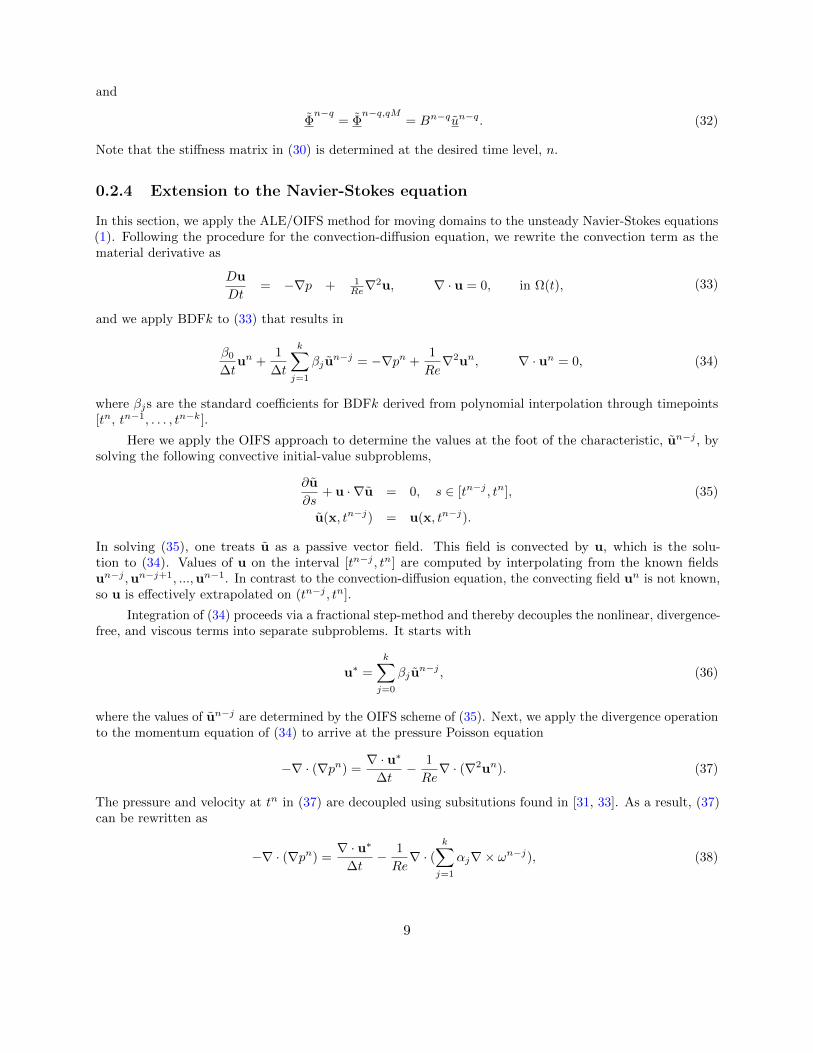
with ω = 5. The mesh consists of a 16× 16 array of square spectral elements. We have inhomogeneousDirchlet conditions on all of ∂Ω corresponding to u (60). In the present case, since we have an exact solutionas a function of space and time, we can run the Dirichlet case with the solution prescribed on all four sides ofthe domain. Starting with the initial condition we take ν = .01 and u = (1, .3) and evolve the solution to afinal time T . Figure 3 shows a picture of the velocity magnitude in the domain at two timepoints.

Figure 4 shows the maximum pointwise error in the x-component of the velocity at a final time ofT = 7.0. The left panel shows that the characteristic scheme yields expected kth-order accuracy for k = 2and 3. The right panel shows the error (using k = 3) as a function of ∆t for several values of N . The generaltrend is that the error is dominated by spatial error for sufficiently small values of ∆t and becomes dominatedby temporal error as ∆t is increased.

Figure 5 shows the maximum pointwise error as a function of the Courant number, C, defined by(56). Results are shown for k = 2 (left) and 3 (right) with a fixed polynomial order of N = 11 in each case.As a result, C becomes a strong function of the chosen timestep, ∆t. Each data point is calculated for atimestep that is fixed for the duration of the simulation. The solution is evolved to T = 1.0, where C is thencalculated. In each panel, we compare error and the maximum C that can be attained for CHAR/BDFk andEXTk/BDFk. For CHAR/BDFk we choose the number of sub-steps to be M = 1 which means ∆s = ∆t.Interestingly, for k = 2 (left) the characteristic scheme (CHAR/BDFk) exhibits a lesser degree of accuracythan its EXTk/BDFk counterpart. On the other hand, the characteristic scheme achieves a Courant number(or timestep) that is more than twice that for EXTk/BDFk. This is almost true for k = 3 (right). Inparticular, the characteristic scheme is able to attain a higher C, although it is not twice as high as theEXTk/BDFk scheme. At their largest timesteps, however, the characteristic scheme is as accurate as theEXTk/BDFk scheme.

0.4.2 Flow in a Channel with a Moving Indentation

In this section we validate our characteristic-based approach by studying the two-dimensional, unsteady flowof a viscous, incompressible fluid in a channel with a time-dependent indentation in one wall. This problem

15

T = 3.5T = 1.5

Figure 3: Eddy solution results (CHAR/BDFk) at Re=100 for the moving domain problem: leftand right images show velocity magnitude and domain configuration at two timepoints with k = 3.

∆t

||u−u|| ∞

PN − PN

N=7

8

9

10

11

∆t

||u−u|| ∞

PN − PN

k = 2

k = 3

Figure 4: Eddy solution results (CHAR/BDFk) at Re=100 for the moving domain problem: (left)2nd- and 3rd-order temporal accuracy based on maximum pointwise error is shown for polynomialorder N = 12, (right) maximum pointwise error for N = 7–11 using k = 3. Dashed line showsthe slope for each BDFk scheme. The slopes agree with temporal accuracy of k = 2 and k = 3,respectively.

has been the subject of several studies [1, 41, 42] seeking to better understand flow in collapsible tubes suchas arteries and veins. The configuration for this study is shown in Fig. 6. Based upon the experiment ofPedley and Stephanoff [41], a steady Poiseuille flow or parabolic velocity profile is prescribed at the inlet. Anindentation on the bottom wall moves in and out sinusoidally where its retracted position is flush with thewall. The two main nondimensional parameters are given by the Reynolds number Re = Uob

ν = 507 and the

Strouhal number St = bUoT

= 0.037. Uo = Qo

b is the mean inlet velocity, where Qo is the volumetric flow rateper unit channel depth and b is the channel height. T is the oscillation period.

The walls of the channel are defined to be at y = b and y = F (x, t). F (x, t) is taken to be of theseperable form

F (x, t) = g(x)h(t), (63)

16

C

||u−u|| ∞

Cmax=1.1321

0.503CCO

C

||u−u|| ∞ Cmax=0.440

AAU

0.819CCO

Figure 5: Eddy solution results (CHAR/BDFk (blue) vs. EXTk/BDFk (red) ) where the solutionis evolved to T = 1.0. Left image shows maximum pointwise error as a function of the Courantnumber, C, for k = 2. Right image is for k = 3.

where h(t) = 0 for t < 0, h(t) ≥ 0 for t ≥ 0 and g(x) ≥ 0. Here we choose h(t) as

h(t) = 0.5[1− cos 2πt∗], (64)

where t∗ = tT . The shape of the indentation is desribed by g(x) and is symmetric around the origin x = 0

(i.e. g(−x) = g(x)). Following the analysis in Ralph and Pedley [42], g(x) is written as

g(x) = 0.5hmax[1− tanh a(|x| − x2)], (65)

which reproduces the wall profiles given by experiments. Here hmax = 0.38b specifies the maximum height ofthe indentation, and a = 4.14. x2 = 0.5(x1 + x3), where x1 = 4b and x3 = 6.5b. The entire length of thechannel is given as l1 + l2 = 40b with l1 = 13.75b and l2 = 26.25b.

Figure 6: Schematic for flow in a channel with a moving-wall indentation.

The development of the flow can be seen in Figs. 7–8 and is similar to the flow field found in theexperiments of Pedley and Stephanoff [41]. At some time between t∗ = 0.20 and t∗ = 0.30 flow separates onthe lee side of the moving indentation, and the resulting eddy grows rapidly. Around t∗ = 0.40, a second

17

Figure 7: Wave formation and propagation downstream of a moving indentation for Re = 507. Thetotal number of elements E = 60 × 8 = 480 with polynomial order N = 11. Results shown forCHAR/BDFk with k=2 and C = 2.

eddy forms on the upper wall. Adopting the convention in the experiment [41], we label the second eddy asB. Trifurcation of eddy B into smaller corotating recirculations can be seen in Figs. 7(g)-(j) and is consistentwith the results found in [42]. Figure 9 tracks the motion of eddy B by measuring the trough position, orlowest point of the eddy along a scaled abscissa coordinate, x∗, over time. The coordinate is defined according

18

Figure 8: Wave formation and propagation downstream of a moving indentation for Re = 507. Thetotal number of elements E = 60 × 8 = 480 with polynomial order N = 11. Results shown forCHAR/BDFk with k=2 and C = 2.

to the analysis of Pedley and Stephanoff [41] and is given by

x∗ =

(x− x1

b

)(10St)( 1

3 ). (66)

The unfilled triangular symbols represent results from the proposed characteristic-based scheme. We note thatresults for the larger Courant number, C = 2, which is realized by a larger timestep, shows good agreeement

19

Figure 9: Space-time (x-t) curve for eddy B. Filled circular symbol represents experimental resultsfrom Pedley and Stephanoff [41]. Unfilled symbols represent lPN − lPN approach. Square symbolrepresents the standard semi-implicit approach EXTk/BDFk. Triangular symbols are based on theproposed characteristic scheme CHAR/BDFk. Results are presented for k=2.

inflow

outflowxyz

Figure 10: Distribution of velocity magnitude for the CHAR/BDFk and lPN − lPN approach on avertical slice at t = 50.

with the experimental results.

0.4.3 Peristaltic Pumping

For the 3D case, verification of the CHAR/BDFk implementation begins with the tubular setup of Fig. 10.The moving mesh in this case generates a peristaltic pumping that strongly influences the temporal andspatial evolution of the velocity field. The pipe has a base radius R = 1/2 and length L = 16. The prescribedmesh velocity is

w1 = −W x

Rcos(kz − ωt), w2 = −W y

Rcos(kz − ωt), w3 = 0, (67)

where W = A/ω is the velocity amplitude and A = 0.1 tanh(0.2z) tanh(0.2t) is the amplitude of thedisplacement. The prescribed wavenumber is k = π/3, and the frequency is ω = 1. The subscripts 1, 2, and3 in (67) correspond to the x, y, and z directions respectively. The Reynolds number is always below 200so that the flow remains laminar. At the inflow a steady parabolic velocity profile with a maximum axialvelocity u3 = 1 at the cylinder center is imposed while at the outflow zero-Neumann boundary conditions are

20

Figure 11: Instantaneous axial velocity profile at T = 50 during peristaltic pumping. Resultsare shown for two cases. The blue line is the benchmark study using the EXTk/BDFk andlPN − lPN−2 approach. Red symbols are for the proposed CHAR/BDFk and lPN − lPN approach.Both simulations have the same number of elements E = 192 and polynomial order N = 9. Resultsare presented for k=2.

Method Time to Solution (Sec.) - BDF2 Time to Solution (Sec.) - BDF3

CHAR/BDFk 2.10× 103 2.53× 103

EXTk/BDFk 5.88× 103 5.97× 103

Table 1: Peristaltic pumping performance. Time-to-solution results are measured at final timetfinal = T = 50. In both cases, the polynomial order is N = 9 and the lPN − lPN formulation isused. For CHAR/BDFk, M = 1 and a maximum stable timestep is chosen such that C > 1.

used. At the pipe walls the velocity is set equal to the mesh velocity in order to prevent a flow across thewalls. The numerical setup including the mesh is given in the example peris of the Nek5000 package.

Figure 11 shows the axial velocity distribution along the centerline of the pipe at time, T = 50.For this calculation, the total number of elements is E = 192 with a polynomial order of N = 9. Thepresent characteristic-based (CHAR/BDFk), lPN − lPN formulation is compared with the non-characteristic(EXTk/BDFk), lPN − lPN−2 approach of Ho and Patera [43, 44]. The circle markers indicate results fromthe CHAR/BDFk approach where the number of RK4 substeps is M = 2 which achieves the C = 2. Theaxial velocity shows excellent agreement between the two formulations.

Table 1 shows time-to-solution data comparing the CHAR/BDFk approach with the EXTk/BDFkapproach using the same lPN − lPN formulation. These calculations were performed on an Apple MacBookPro which runs a 2.3 GHz Intel Core i7 processor. Using M = 1, we chose a maximum timestep such thatthe calculation remains numerically stable. This results in a C > 1. As the table shows, the characteristicapproach achieves a reduction in the time to solution by more than a factor of 2 over the noncharacteristicapproach.

21

0.4.4 TCC-III Engine

In this section, we illustrate a practical application of the CHAR/BDFk method. In particular, we assessthe performance of this approach in a simulation of incompressible flow during the intake stroke for theTransparent Combustion Chamber-III (TCC-III) engine [7]. For this investigation, we modify the geometryof the TCC-III engine by simulating flow that enters an intake-valve and empties into a pancake-shapedcombustion chamber. The image on the left of Fig. 12 is a schematic describing the geometry. During theintake stroke, the valve opens (i.e., moves down) thus allowing fluid to enter into the combustion chamber.As the valve moves down, the piston is simultaneously moving downward with velocity, vpiston. The diameterof the cylinderical combustion chamber, known as the bore, represents the characteristic length, Lo. Thediagram on the right shows the geometric layout for the piston pin (P), crank pin (N) and crank center (O).The piston pin is connected to the crank pin through a connecting rod of length, l. Here x is the piston pinposition, r is the crank radius (also called the half stroke), and a is the crank angle which is measured fromthe bore centerline or the top dead center (TDC) position of the piston. The crankshaft angular velocity, ω, isrelated to the engine revolutions per minutes (RPM) by ω = 2πRPM

60 . Assuming a constant angular velocity,the crank angle is given by a = ωt. The position of the piston, x, and the velocity, vpiston, are given as

x = r cos a+√l2 − (r sin a)2,

vpiston =dx

da× da

dt=

(−r sin a− r2 sin a cos a√

l2 − r2 sin2 a

)× ω. (68)

Figure 13 illustrates the piston velocity and the motion of the intake valve. The valve motion from the onlinedatabase [45] is described in terms of the valve lift (i.e. distance from the horizontal chamber walls) versusthe crank-angle (CA) degree.

The reference velocity for this calculation is the maximum piston speed, Uo = vpiston,max. Based uponFig. 13, the maximum piston speed occurs at approximately 440o CA, as the piston is moving downwardtoward the bottom dead center (i.e., lowest position). DNS calculations are shown in Fig. 14, whichshow non-dimensional velocity distribution snapshots for Re = 5000. For this DNS we use the followingparameters: RPM = 50, Bore (Lo) = 9.2 cm, Stroke (2r) = 8.6 cm, Rod length (l) = 23.10 cm, andvpiston,max = 22.90 cm/s. According to the snapshots, we observe a fluid entering the pancake-shapedchamber and evolves into a highly complex and turbulent flow field. Developing a turbulent flow field insidethe chamber is crucial to preparing the fuel mixture for combustion [5].

The simulation begins at 362o CA, where the initial condition is a quiescent flow. The moving boundariesfor this problem are the valve and piston surface, while the remaining boundaries (cylindrical chamber) areconsidered to be static walls. Due to the incompressible assumption, the inflow boundary condition (at thetop of the intake-valve) is imposed such that the volumetric flow rate is the same as the volumetric change inthe chamber due to the piston motion. This ensures that flow enters the valve and cylindrical chamber asthe piston surface moves downward. These results were captured by using the CHAR/BDF3 scheme with atarget Courant number of C = 3 and setting M = 3. The total number of spectral elements used is E = 6784with polynomial order of N = 11.

The mesh displacement is computed by integrating Eq. (21) in time where the mesh velocity w issubject to the kinematic condition,

w · n|∂Ω = u · n|∂Ω. (69)

where n is the unit normal at the domain surface, ∂Ω(t). In order to smoothly blend boundary data into thedomain interior we solve Laplace’s equation (i.e., −∇·µ∇u = 0) in order to blend the surface velocities to theinterior, relying on the maximum principle to give a bounded interpolant. Here, u represents a displacementfactor which is applied at all gridpoints in the domain.

To preserve the resolution of critical boundary-layer elements, we increase the diffusivity (µ) near specificwalls so that the mesh velocity tends to match that of the nearby object. The bulk of the mesh deformation

22

Figure 12: Schematic for the modified TCC-III internal combustion engine (Left). The image onthe right is a diagram showing the geometric layout of the piston pin (P), crank pin (N) and crankcenter(O).

is effectively pushed into the far field, where elements are larger and thus better able to absorb significantdeformation. The idea of using variable diffusivity has been explored in finite-element contexts where thecoefficient is based on local element volumes (e.g., [46, 47]) and can also be applied to the elasticity equations.

We set µ(x) = 1 + αe−δ2

with α = 3 and δ := d/∆ the distance to the wall normalized by a chosenlength scale, ∆. In the absence of any other scale information, we set ∆ equal to the average thicknessof the first layer of spectral elements in contact with the given object. To compute d, we use a Euclidiangraph-based approximation to the true distance function. A variable diffusivity is especially beneficial inthe vicinity of the valve and piston surfaces since boundary motion is in the same direction as the normalto the surface. Note, boundary motion along the cylinder chamber is orthogonal to the surface where theboundary-layer is preserved throughout the entire simulation.

0.4.5 TCC-III Engine: Computational Performance

We use this section to illustrate the performance for the CHAR/BDFk scheme by monitoring the computationalcost or wall time required to execute an early phase of the intake stroke from 362o CA to 375o CA. The earlyphase of the intake stroke is critical in the evolution of the flow due to the fluid’s dramatic acceleration in thesmall valve-gap region (also known as the valve seat). The high-speed flow in this region has a lasting effecton the evolution of the flow structure in the chamber. Figure 15 illustrates this phenomena by showing thenondimensional velocity distributions for 364o CA (left) and 375o CA (right). From the figure, we observethat the largest velocities exist in the small-gap region. In terms of computational performance, it becomescritical for the practitioner to choose a timestepping scheme that attains the largest stable Courant number,C.

Figure 16 shows the wall-time results for the simulation to execute from 362o CA to 375o CA. Thesecalculations were performed on 4096 processors of an IBM BG/Q machine maintained by the ArgonneLeadership Computing Facility. The gain in using the CHAR/BDFk scheme is notable, where we see that itdelivers results sooner than the EXTk/BDFk scheme. Early in the simulation ( CA < 363o), the CHAR/BDFkscheme shows little gain which is likely due to the piston velocity being relavitvely small. However, it’sadvantage becomes apparent at larger CA where we see a notable difference in the time-to-solution. The

23

Figure 13: Intake-Valve and Piston surface motion. The red line indicates the valve-lift distancewhile the blue line shows the piston velocity. Both are functions of the crank-angle.

influence of the CHAR/BDFk scheme is particularly dramatic for C = 1 or 2. Indeed, figure 17, shows thespeedup as a function of the crank-angle (CA) degree. In this work, we define speedup as the ratio

speedup =Time-To-Solution (EXTk/BDFk)

Time-To-Solution (CHAR/BDFk), (70)

where the numerator and denominator signify that the method being used is the noncharacteristic (EXTk/BDFk)and characteristic (CHAR/BDFk) method, respectively. At approximately 365o CA, the maximum speedupis achieved. Using CHAR/BDFk we gather the timing information at 375o CA and note the overall speedupof 2.7 (for target C=4) over the EXTk/BDFk scheme which is limited to a stable Courant number of C = 0.5.For a target Courant number of C ≥ 2 we observe that a speedup factor of at least 2 is attained.

Figure 18 shows the change in the timestep ∆t over the course of the simulation. As expected we canachieve larger (and more stable) timesteps with higher C (or M - number of Runge-Kutta timesteps). Thelarge drop in the timestep size for CA > 364 is due to the large flow velocities which are moving through thevalve-seat region. While the overall average timestep increases by a factor of approximately 8, the wall-timeresults show the effect of diminishing returns due, in part, to the additional number (M) of Runge-Kuttatimesteps between each foot along the characteristic. In addition, the influence on wall time is affected bythe number of pressure iterations, which can be seen in figure 19. Due to larger timesteps, the number ofpressure iterations in the preconditioned conjugate gradient algorithm increases which adds to the overallcomputational work that is performed for each timestep. Nonetheless, these results illustrate the advantageof the characteristics/OIFS scheme, which shows a a reduction in computational time over standard methodsby more than a factor of two.

0.4.6 A Pinched Pipe

In order to assess the limits and benefits of our characteristic-based approach, we conduct a simple exerciseof a pinched or constricted pipe. A schematic can be seen in figure 20, where the axial boundary undergoesa radial constriction. The center of the pipe (along the axial direction) undergoes the maximum radial

24

constriction and the effect is observed linearly towards the ends (i.e. inlet and outlet). As a real-life analogue,one may imagine the local constriction of a garden hose as water is rushing through it. If we consider aincompressible fluid entering the pipe at a fixed flow rate then the constriction will increase the velocity ofthe fluid as it passes through the pipe. Computationally, a singularity in the mesh would occur if constrictionproceed without bound. This would mean that ∆xmin → 0 as time proceeds. As such, the Courant number(56), would increase for a fixed timestep.

Our aim in this section is to assess if our implementation of the CHAR/BDFk approach can realizeCourant numbers larger than the stable Courant numbers for EXTk/BDFk. In order to do this, we track theCourant number in time for the constricted pipe. We fix our timestep and change the number of RK4 substeps(i.e. M) that are being performed. Figure ?? compares the realized Courant number for a given temporaldiscretization. In each case, the Courant number is calculated at each timestep until the algorithm becomesnumerically unstable and produces diverging/erroneous results. This occurs because of the mesh singularityin the mid-axial plane of the pipe. The top left image of figure ?? shows the realized Courant numbers for theEXTk/BDFk scheme. This plot shows how the solution becomes unstable at Courant numbers that are wellbelow 10. In fact, the stable Courant number for EXTk/BDFk is known to be approximately 0.5. Courantnumbers that are larger than 0.5 are past the stability limit and producing erroneous results. The other plotsshow achievable Courant numbers using the CHAR/BDFk scheme for M = 1, 2, 3, 4 and 8. As the plots show,a larger value for M will achieve a higher Courant number. It is worth noting that while the x-axis indicatesthe temporal variable, it is also an indication of the change in radius for the smallest cirucular cross-section(i.e. mid-axial plane) of the pipe. That said, these plots suggest that a larger M also provides the user withthe means to capture flow-fields in the small grid limit without changing the timestep (∆t). To confirmthat behavior, figure 21 shows the smallest gap that is being achieved for a given timestep and temporaldiscretization. Timestep values are the same as the ones that are used in figure 23. The gap (ordinate)compares the minimum radius to the original radius at the start of the simulation. The circular symbol showsthe results for EXTk/BDFk which attains the largest gaps before numerical instability occurs. The othersymbols show results for CHAR/BDFk. Larger values for M show that the smaller gaps are achieved for agiven timestep. Figure 22 shows the maximum value for the axial component of the velocity versus time.Similar to figure 23, we plot this component until the solution becomes numerically unstable. We confirmthat larger velocities are captured for the CHAR/BDFk schemes versus the EXTk/BDFk scheme.

0.5 Appendix

0.5.1 Outflow Boundary Condition

This section illustrates the unique outflow boundary condition that was used in the peristaltic pumpingexample of section 0.4.3. The so-called turbulent outflow boundary condition [48] is currently employed inorder to avoid the locally negative flux at the outflow boundary. Such negative fluxes may occur in turbulentflows where vortices might allow for flow characteristics to enter into the domain rather than exit. As isnoted in [48], the incoming characteristics can rapidly lead to numerical instability. In order to avoid thisphenomena, a mean axial component to the velocity field is added to the layer of element adjacent to theoutflow boundary. This is effectively accomplished by added a divergence in the velocity field to this layer ofelements. In particular, this divergence is set so that it ramps from zero at the upstream end of the layer to afixed positive value at the exit.

The effect on the flow field is only noticed at this last layer of elements and does not effect the otherparts of the domain where the interest of the study remains. In the peris example, there are no incomingcharacteristics which lead to instabilities. We investigate if the turbulent outflow boundary condition doesdrastically affect the flow-field. Figure 24 shows the results for the persitaltic pumping example with theturbulent outflow boundary condition. In particular, the top row shows the axial velocity along the centerlineof the domain. Each plot compares the EXTk/BDFk (IFCHAR = F) scheme with the CHAR/BDFk

25

(IFCHAR = T) scheme. The left image shows the situations when the turbulent outflow boundary conditionis employed. In this image, can see the sharp rise in the axial velocity. The right image shows the smoothaxial profile without the turbulent outflow boundary condtion. One can see that the upstream profile isunaffected by the additional divergence. The second row shows the maximum axial velocity in the entiredomain over a given time period. When the special boundary condition is employed one can see the largervalues for velocity which is due to the added divergence. Similar phenomena can be seen in Figure 25 for thepressure.

26

0.5.2 Material Derivative of the Jacobian

dJ(r, t)

dt= εijk

∂

∂r1

(dxidt

)∂xj∂r2

∂xk∂r3

+ εijk∂xi∂r1

∂

∂r2

(dxjdt

)∂xk∂r3

+ εijk∂xi∂r1

∂xj∂r2

∂

∂r3

(dxkdt

)= εijk

∂

∂r1(wi)

∂xj∂r2

∂xk∂r3

+ εijk∂xi∂r1

∂

∂r2(wj)

∂xk∂r3

+ εijk∂xi∂r1

∂xj∂r2

∂

∂r3(wk)

= εijk∂wi∂xm

(∂xm∂r1

)∂xj∂r2

∂xk∂r3

+ εijk∂xi∂r1

∂wj∂xm

(∂xm∂r2

)∂xk∂r3

+ εijk∂xi∂r1

∂xj∂r2

∂wk∂xm

(∂xm∂r3

)= εijk

∂w1

∂x1

(∂xi∂r1

)∂xj∂r2

∂xk∂r3

+ εijk∂xi∂r1

∂w2

∂x2

(∂xj∂r2

)∂xk∂r3

+ εijk∂xi∂r1

∂xj∂r2

∂w3

∂x3

(∂xk∂r3

)=

∂w1

∂x1J(r, t) +

∂w2

∂x2J(r, t) +

∂w3

∂x3J(r, t)

= (∇ ·w)J(r, t) (71)

0.6 Conclusions

A new characteristic-based spectral element method has been introduced for incompressible flows in moving-domain problems. By adopting a taylored form of the operator-integration-factor-splitting (OIFS) scheme,this method decouples the nonlinear and linear terms in the unsteady Navier-Stokes equations and reducetimestepping constraints compared to the standard semi-implicit schemes. In conjunction with the lPN − lPNformulation, we show 2nd- and 3rd-order temporal convergence rates for our characteristic-based scheme anddemonstrate good agreement with physical experiments with small variation in the results as target Courantnumbers are increased. We apply our method for direct numerical simulations (DNS) of turbulent flow fieldsto study the intake stroke of the modified TCC-III engine. Performance results for resolving fast-moving flowthrough the small-gap region of the intake valve from 362o to 375o CA indicate that the characteristic-basedmethod can reduce the time to solution by more than a factor of 2.

27

365o CA 385o CA

405o CA 425o CA

445o CA 465o CA

Figure 14: TCC-III Engine. Centerplane, non-dimensional velocity magnitude distribution for thelPN − lPN approach. Results were determined using the CHAR/BDFk scheme with a CFL = 3.Top Row: 365o, and 385o CA (Left to Right); 405o, and 425o CA (Left to Right - Middle Row);445o and 465o CA (Left to Right - Bottom Row)

28

364o CA 375o CA

Figure 15: Closeup view of the intake valve. Centerplane, nondimensional velocity distributionsduring an intake stroke for an incompressible flow at CA 364o (left) and 375o (right). Re = 5000.

Figure 16: Wall Time (vertical-axis) since start of engine simulation (left). x-axis represents CA,crank-angle degrees. Polynomial order is N = 11 with a BDF3 temporal discretization. Calculationsare carried out from 362o CA to 375o CA. The inset shows speedup for the CHAR/BDFk forconsecutively large Courant number C. Speed-up is defined by Eq. (70). Note: piston velocityfor CA < 364 is nearly zero due to TDC position of the piston (i.e. small piston velocity), thuscontributing to comparable wall-time results for CA < 364. These results were found using 4096processors on Cetus - an IBM BG/Q machine maintained by the Argonne Leadership ComputingFacility.

29

Figure 17: Speed-Up (vertical axis) since start of engine simulation (left). x-axis represents CA,crank-angle degrees. Polynomial Order is N = 11 with a BDF3 temporal discretization. Calculationsare carried out from 362o CA to 375o CA. Speed-up is defined by Eq. (70). These results were foundusing 4096 processors on Cetus - an IBM BG/Q machine maintained by the Argonne LeadershipComputing Facility.

Figure 18: ∆t (vertical-axis) as a function of CA. Results show how a variable timesteppingimplementation changes with the choice of C that is used for the CHAR/BDFk method. Polynomialorder is N = 11 with a BDF3 temporal discretization.

30

Figure 19: Pressure iterations as a function of crank-angle degree for 362o–375o CA. The peaks inthe figure represent the effect of the restart procedure.

Figure 20: Schematic for a pinched pipe.

31

Figure 21: Constricted Pipe. Smallest achievable radius before time-stepping became unstable andproduced diverging results.

32

Figure 22: Constricted Pipe. Axial Velocity versus time.

33

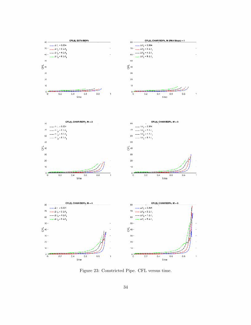
Figure 23: Constricted Pipe. CFL versus time.

34

Figure 24: Turbulent Outflow Boundary Condition Phenomena: The effect on axial velocity for theperistaltic pump.

35

Figure 25: Turbulent Outflow Boundary Condition Phenomena: The effect on pressure for theperistaltic pump.

36

Bibliography

[1] I. Demirdzic, M. Peric, Finite volume method for prediction of fluid flow in arbitrarily shaped domainswith moving boundaries, International Journal for Numerical Methods in Fluids 10(7), 771 (1990)

[2] T. Tezduyar, M. Behr, J. Liou, A new strategy for finite element computations involving movingboundaries and interfaces–the dsd/st procedure: I. the concept and the preliminary numerical tests,Computer Methods in Applied Mechanics and Engineering 94(3), 339 (1992)

[3] T.E. Tezduyar, M. Behr, S. Mittal, J. Liou, A new strategy for finite element computations involvingmoving boundaries and interfacesthe deforming-spatial-domain/space-time procedure: Ii. computationof free-surface flows, two-liquid flows, and flows with drifting cylinders, Computer methods in appliedmechanics and engineering 94(3), 353 (1992)

[4] J. Donea, A. Huerta, J.P. Ponthot, A. Rodrguez-Ferran, Arbitrary LagrangianEulerian methods, Ency-clopedia of computational mechanics DOI: 10.1002/0470091355.ecm009, 1:14 (2004)

[5] C. Arcoumanis, J. Whitelaw, Fluid mechanics of internal combustion enginesa review, Proceedings ofthe Institution of Mechanical Engineers, Part C: Journal of Mechanical Engineering Science 201(1), 57(1987)

[6] T.W. Kuo, X. Yang, V. Gopalakrishnan, Z. Chen, Large eddy simulation (les) for ic engine flows, OilGas Sci. Technol.–Rev. IFP Energies nouvelles (2012)

[7] P. Schiffmann, S. Gupta, D. Reuss, V. Sick, X. Yang, T.W. Kuo, Tcc-iii engine benchmark for large-eddysimulation of ic engine flows, Oil & Gas Science and Technology 71(1) (2016)

[8] C. Rutland, Large-eddy simulations for internal combustion engines–a review, International Journal ofEngine Research p. 1468087411407248 (2011)

[9] M. Schmitt, C.E. Frouzakis, A.G. Tomboulides, Y.M. Wright, K. Boulouchos, Direct numerical simulationof multiple cycles in a valve/piston assembly, Physics of Fluids 26(3), 035105 (2014)

[10] M. Schmitt, C. Frouzakis, Y. Wright, A. Tomboulides, K. Boulouchos, Investigation of wall heat transferand thermal stratification under engine-relevant conditions using DNS, Int. J. of Engine Res. 17(1), 63(2016)

[11] A. Patera, A spectral element method for fluid dynamics : laminar flow in a channel expansion, J.Comput. Phys. 54, 468 (1984)

[12] L. Ho, A Legendre spectral element method for simulation of incompressible unsteady viscous free-surfaceflows. Ph.D. thesis, Massachusetts Institute of Technology (1989). Cambridge, MA.

[13] L. Ho, Y. Maday, A. Patera, E. Rønquist, A high-order Lagrangian-decoupling method for the incom-pressible Navier-Stokes equations, Comput. Methods Appl. Mech. Engrg. 80, 65 (1990)

[14] L. Ho, A. Patera, A Legendre spectral element method for simulation of unsteady incompressible viscousfree-surface flows, Comput. Methods Appl. Mech. Engng. 80, 355 (1990)

37

[15] P. Fischer, M. Schmitt, A. Tomboulides, Recent developments in spectral element simulations of moving-domain problems, Fields Institute Communications: Recent Progress and Modern Challenges in AppliedMathematics, Modelling and Computational Science Springer/Fields Institute (2016)

[16] S. Orszag, M. Israeli, M. Deville, Boundary conditions for incompressible flows., J. Sci. Comp. 1, 75(1986)

[17] Y. Maday, A. Patera, E. Rønquist, An operator-integration-factor splitting method for time-dependentproblems: Application to incompressible fluid flow, J. Sci. Comput. 5, 263 (1990)

[18] A. Tomboulides, M. Israeli, G. Karniadakis, Efficient removal of boundary-divergence errors in time-splitting methods, J. Sci. Comput. 4, 291 (1989)

[19] J. Perot, An analysis of the fractional step method, J. Comp. Phys. 108, 51 (1993)

[20] W. Couzy, Spectral element discretization of the unsteady Navier-Stokes equations and its iterativesolution on parallel computers. Ph.D. thesis, Swiss Federal Institute of Technology-Lausanne (1995).Thesis nr. 1380

[21] P. Fischer, An overlapping Schwarz method for spectral element solution of the incompressible Navier-Stokes equations, J. Comput. Phys. 133, 84 (1997)

[22] P. Fischer, J. Lottes, in Domain Decomposition Methods in Science and Engineering Series, ed. byR. Kornhuber, R. Hoppe, J. Priaux, O. Pironneau, O. Widlund, J. Xu (Springer, Berlin, 2004)

[23] J.W. Lottes, P.F. Fischer, Hybrid multigrid/Schwarz algorithms for the spectral element method, J. Sci.Comput. 24, 45 (2005)

[24] H. Tufo, P. Fischer, Fast parallel direct solvers for coarse-grid problems, J. Parallel Distrib. Comput. 61,151 (2001)

[25] P. Fischer, J. Lottes, W. Pointer, A. Siegel, Petascale algorithms for reactor hydrodynamics, J. Phys.Conf. Series 125, 012076 (2008)

[26] J. Lottes, Independent quality measures for symmetric AMG components. Tech. Rep. ANL/MCS-P1820-0111, Argonne National Laboratory, Argonne, IL, USA (2011)

[27] J. Boyd, Two comments on filtering for Chebyshev and Legendre spectral and spectral element methods,J. Comput. Phys. 143, 283 (1998)

[28] P. Fischer, J. Mullen, Filter-based stabilization of spectral element methods, Comptes rendus del’Academie des sciences, Serie I- Analyse numerique 332, 265 (2001)

[29] J. Malm, P. Schlatter, P. Fischer, D. Henningson, Stabilization of the spectral-element method inconvection dominated flows by recovery of skew symmetry, J. Sci. Comp. 57, 254 (2013)

[30] H. Tufo, P. Fischer, in Proc. of the ACM/IEEE SC99 Conf. on High Performance Networking andComputing, Gordon Bell Prize (IEEE Computer Soc., CDROM, 1999)

[31] M. Deville, P. Fischer, E. Mund, High-Order Methods for Incompressible Fluid Flow (CambridgeUniversity Press, Cambridge, 2002)

[32] O. Pironneau, On the transport-diffusion algorithm and its applications to the Navier-Stokes equations,Numer. Math. 38, 309 (1982)

[33] A. Tomboulides, J. Lee, S. Orszag, Numerical simulation of low Mach number reactive flows, Journal ofScientific Computing 12, 139 (June 1997)

[34] P. Fischer, Projection techniques for iterative solution of Ax = b with successive right-hand sides,Comput. Methods Appl. Mech. Engrg. 163, 193 (1998)

38

[35] P. Fischer, N. Miller, H. Tufo, in Parallel Solution of Partial Differential Equations, ed. by P. Bjørstad,M. Luskin (Springer, Berlin, 2000), pp. 158–180

[36] S. Orszag, Spectral methods for problems in complex geometry, J. Comput. Phys. 37, 70 (1980)

[37] P. Fischer, Spectral element solution of the Navier-Stokes equations on high performance distributed-memory parallel processors. Ph.D. thesis, Massachusetts Institute of Technology (1989). Cambridge,MA.

[38] Y. Maday, A. Patera, in State-of-the-Art Surveys in Computational Mechanics, ed. by A. Noor, J. Oden(ASME, New York, 1989), pp. 71–143

[39] P. Fischer, in 22nd AIAA Computational Fluid Dynamics Conference, AIAA Aviation (AIAA 2015-3049,2015)

[40] O. Walsh, in The NSE II-Theory and Numerical Methods, ed. by J. Heywood, K. Masuda, R. Rautmann,V. Solonikkov (Springer, 1992), pp. 306–309

[41] T. Pedley, K. Stephanoff, Flow along a channel with a time-dependent indentation in one wall: thegeneration of vorticity waves, Journal of Fluid Mechanics 160, 337 (1985)

[42] M. Ralph, T. Pedley, Flow in a channel with a moving indentation, Journal of Fluid Mechanics 190, 87(1988)

[43] L. Ho, A. Patera, A legendre spectral element method for simulation of unsteady incompressible viscousfree-surface flows, Comput. Methods Appl. Mech. Engrg. 80, 355 (1990)

[44] L. Ho, A Legendre spectral element method for simulation of incompressible unsteady viscous free-surfaceflows. Ph.D. thesis, Massachusetts Institute of Technology (1989). Cambridge, MA.

[45] V. Sick, D. Reuss, X. Yang, T.W. Kuo. TCC-III CFD Input Dataset.https://deepblue.lib.umich.edu/handle/2027.42/108382

[46] A. Masud, T.J.R. Hughes, A space-time galerkin/least-squares finite element formulation of the Navier-Stokes equations for moving domain problems, Comput. Methods Appl. Mech. Engrg. 146, 91 (1997)

[47] H. Kanchi, A. Masud, A 3d adaptive mesh moving scheme, Int. J. Numer. Methods Fluids 54, 923 (2007)

[48] P. Fischer, F. Loth, S. Lee, D. Smith, H. Bassiouny, Simulation of high Reynolds number vascular flows,Comput. Methods Appl. Mech. Engrg. 196, 3049 (2007)

39

Acknowledgments

This material is based upon work supported by the U.S. Department of Energy, Office of Science, Offices of Advanced Scientific Computing Research, under Contract DE-AC02-06CH11357. The research also used resources of the Argonne Leadership Computing Facility, which is supported by the U.S. Department of Energy, Office of Science, under Contract DE-AC02-06CH11357.

Argonne National Laboratory is a U.S. Department of Energy laboratory managed by UChicago Argonne, LLC

Argonne Leadership Computing Facility Argonne National Laboratory 9700 South Cass Avenue, Bldg. 240 Argonne, IL 60439

www.anl.gov