An Open-Source Phase Vocoder with Some - Music Informatics

An Open-Source Phase Vocoder with SomeNovel Visualizations

Kyung Ae Lim

Primary Advisor: Professor Chris Raphael

Secondary Advisor: Dr. Ian Knopke

Capstone ProjectMusic Informatics

School of InformaticsIndiana University Bloomington

June, 2007

Abstract

This project is a phase vocoder implementation that uses multiple, synchronized visual

displays to clarify aspects of the involved signal processing techniques. The program can do

standard phase vocoder operations such as time-stretching and pitch-shifting which are based

on an analysis and resynthesis method using Short-Term Fourier Transform. Conventional 2-

D displays of digital audio including spectrograms, waveform displays and various frequency

domain representations are involved as well as novel 3-D visualizations of frequency domain

are adopted to aid users who begin to learn digital signal processing and phase vocoder.

This application is intend to serve as an open-source educational tool in the near future.

Acknowledgement

I deeply thank Dr. Ian Knopke for his leading on this project and teaching me great

amout of knowledge with his patience and efforts. I have learned not only digital signal

processing and programming technique in music application development, but also the way

of handling and solving difficult problems with positive attitude. To my advisor Professor

Chris Raphael and to Professor Don Byrd, I would like to acknowledge their efforts on

teaching me new, interesting and challenging studies of Music Informatics. I, as the first

student in the program, am indebted so much to both of them. I also thank Professor Steve

Myers and Professor Erik Stolterman for their teaching and supports during the capstone

project period.

Special thanks goes to my husband, Pilsoo Kang, for his endless encouragement and

support, as well as his guide on how to think and work as a scientist. At last, I am grateful for

the cares that I have received from my parents and brother, Linda Lamkin, Sarah Cochran,

David Bremer and Hyo-seon Lee.

1

Contents

1 Introduction 3

2 The Phase Vocoder 52.1 Analysis . . . . . . . . . . . . . . . . . . . . . . . . . . . . . . . . . . . . . . 62.2 Processing and Resynthesis . . . . . . . . . . . . . . . . . . . . . . . . . . . 10

3 System Overview 14

4 Visualizations 20

5 Results and Discussion 25

6 Future work 29

A Phase vocoder pseudocodes 33A.1 Common variables . . . . . . . . . . . . . . . . . . . . . . . . . . . . . . . . 33A.2 Analysis . . . . . . . . . . . . . . . . . . . . . . . . . . . . . . . . . . . . . . 33A.3 Processing and resynthesis: time-stretching . . . . . . . . . . . . . . . . . . . 34A.4 Processing and resynthesis: pitch-shifting . . . . . . . . . . . . . . . . . . . . 35

2

Chapter 1

Introduction

The phase vocoder (7) is an important tool in signal processing, and has become a valuable

part of computer music-making in general (16). Developing on the basic ideas of the earlier

channel vocoder (5), the phase vocoder uses information about the relationships between

sinusoids to obtain a more accurate sound “snapshot” than is normally available using only

a Fourier transform. With the advent of affordable desktop computers, it is now possible

for anyone to have access to this powerful tool, once only available in the most exclusive

research centers.

However, while the phase vocoder can now be found in many educational contexts, it is

difficult for many beginners to grasp. In our experience, while the basic concepts introduced

in most tutorials (4; 1) are not too difficult, the math involved can be daunting, especially if

the student’s background tends more towards music than engineering. This is compounded

by the combination of the multiple different signal processing concepts that make up the

phase vocoder, such the Fourier Transform, signal processing windows, and even interpola-

3

tion techniques. Actually implementing a working phase vocoder is even more difficult and

requires a number of additional “tricks” that are less than obvious (3; 15; 6).

The program described here is intended to help solve some of these difficulties. Several

goals are being addressed here. The first is to create the phase vocoder implementation

that can demonstrate the fundamental concepts in a way that is easier for the newcomer

to understand signal processing. The primary tool here is the use of multiple synchronized

visual displays, in coordination with sound playback. Existing sound files can be modified

using time-stretching and pitch-shifting techniques and saved to new files. The program is

also meant to provide a clear implementation, with comments, that can help a beginner to

understand the implementation details that may not be clear from simply understanding

the mathematics. Finally, we have developed some novel visual representations of frequency

spectrum information that make use of three-dimensional modeling techniques. These pro-

vide new ways to view sound information, and are especially effective in combination with

other more common signal processing visualizations.

4

Chapter 2

The Phase Vocoder

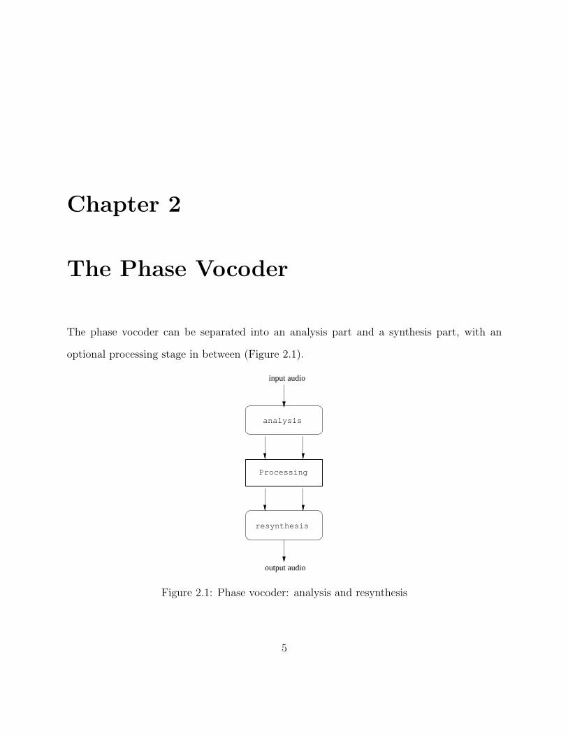
The phase vocoder can be separated into an analysis part and a synthesis part, with an

optional processing stage in between (Figure 2.1).

input audio

output audio

analysis

Processing

resynthesis

Figure 2.1: Phase vocoder: analysis and resynthesis

5

2.1 Analysis

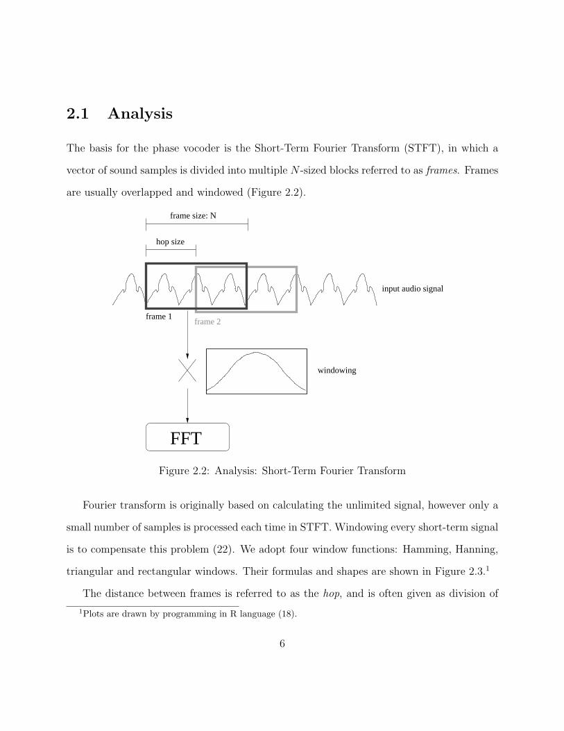
The basis for the phase vocoder is the Short-Term Fourier Transform (STFT), in which a

vector of sound samples is divided into multiple N -sized blocks referred to as frames. Frames

are usually overlapped and windowed (Figure 2.2).

input audio signal

frame 1frame 2

hop size

FFT

frame size: N

windowing

Figure 2.2: Analysis: Short-Term Fourier Transform

Fourier transform is originally based on calculating the unlimited signal, however only a

small number of samples is processed each time in STFT. Windowing every short-term signal

is to compensate this problem (22). We adopt four window functions: Hamming, Hanning,

triangular and rectangular windows. Their formulas and shapes are shown in Figure 2.3.1

The distance between frames is referred to as the hop, and is often given as division of

1Plots are drawn by programming in R language (18).

6

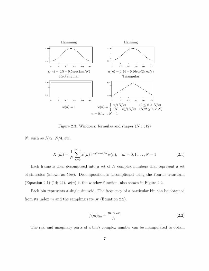
Hamming Hanning

w(n) = 0.5 − 0.5cos(2πn/N) w(n) = 0.54 − 0.46cos(2πn/N)

Rectangular Triangular

w(n) = 1 w(n) =

{

n/(N/2) (0 ≤ n < N/2)(N − n)/(N/2) (N/2 ≤ n < N)

n = 0, 1, ..., N − 1

Figure 2.3: Windows: formulas and shapes (N : 512)

N . such as N/2, N/4, etc.

X (m) =1

N

N−1∑

n=0

x (n) e−j2πnm/Nw(n), m = 0, 1, . . . , N − 1 (2.1)

Each frame is then decomposed into a set of N complex numbers that represent a set

of sinusoids (known as bins). Decomposition is accomplished using the Fourier transform

(Equation 2.1) (14; 24). w(n) is the window function, also shown in Figure 2.2.

Each bin represents a single sinusoid. The frequency of a particular bin can be obtained

from its index m and the sampling rate sr (Equation 2.2).

f(m)bin =m × sr

N(2.2)

The real and imaginary parts of a bin’s complex number can be manipulated to obtain

7

the magnitude and phase of each sinusoid (Equation 2.3).

|X(m)| =√

XR(m)2 + XI(m)2 (2.3)

6 X(m) = tan−1XI(m)

XR(m), where tan−1(x) ∈ [−π, π] (2.4)

Each sinusoid is completely described by these three pieces of information.

The frequency of each bin is fixed, at equally-spaced intervals up to the Nyquist rate (half

the sampling rate). Sinusoids that fall between bin frequencies have their energy distributed

across the surrounding bins. In other words, a single bin frequency is usually only an

approximation of the true frequency of the represented sinusoid. One of the main innovations

of the phase vocoder is that the difference in phases of a particular bin across two successive

frames can be used to derive an adjustment factor (Equation 2.5).

φ(m) =

[

6 X(m) − 6 X(m − 1)

]π

−π

× (sr/2πN) (2.5)

This can then be added to the original approximate frequency to obtain an improved

frequency estimate (Equation 2.6).

f(m)instantaneous = f(m)bin + φ(m) (2.6)

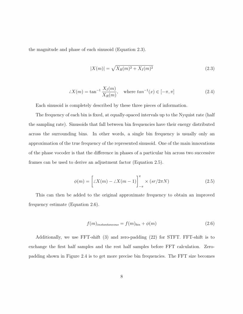
Additionally, we use FFT-shift (3) and zero-padding (22) for STFT. FFT-shift is to

exchange the first half samples and the rest half samples before FFT calculation. Zero-

padding shown in Figure 2.4 is to get more precise bin frequencies. The FFT size becomes

8

larger than frame size and the added samples have 0’s for their values.

frame size

FFT

o o o o o o o o o o o o o o o ozero−padding

FFT size

Figure 2.4: Fourier transform with zero-padding

The analysis algorithm in the phase vocoder is follwing steps;

1. Take frmae(N) size samples from input sound. Store them into a frame buffer.

2. Choose a proper window and window the buffer

3. Zero-pad the buffer

4. FFT-shift the zero-padded buffer.

5. Decompose the buffer by Fourier transform

6. Calculate and store magnitude and phase (output from analysis that is used in resyn-

thesis).

7. Go back to step 1 and start taking frame size sample located at hop size distant from

the first sample of the previous loop.

9

2.2 Processing and Resynthesis

The synthesis stage is basically the analysis stage in reverse: a list of sinusoids in com-

plex number representations are converted resynthesized using an inverse Fourier transform

(IFFT) into a sound signal. While resynthesis can be accomplished using other techniques,

such as direct additive synthesis, the IFFT method is much faster, and with today’s com-

puters can easily be done in real time.

If the output of the analysis stage is used directly for resynthesis, the result will be the

original sound file with no perceptible difference from the original (and we would have nothing

more than a very computationally-expensive way to copy sound information). However, one

of the strengths of the phase vocoder is the possibility of introducing additional processing

between the analysis and synthesis stages.

Unlike time-domain procedures, phase vocoder operations are undertaken in the fre-

quency domain, and can be used to achieve a variety of effects that are difficult or impossible

using other means. Two common techniques are time stretching and pitch shifting. Time

stretching works by using a resynthesis hop size that differs from the analysis hop size, and

also repairing the phase information to produce an expansion or contraction of the sound

file without altering the pitch. Pitch shifts are accomplished in a similar manner to time

stretching, with the additional step of interpolating or decimating the resulting samples to

obtain the original file length (i.e. no time stretch), but with a lower or higher pitch. The

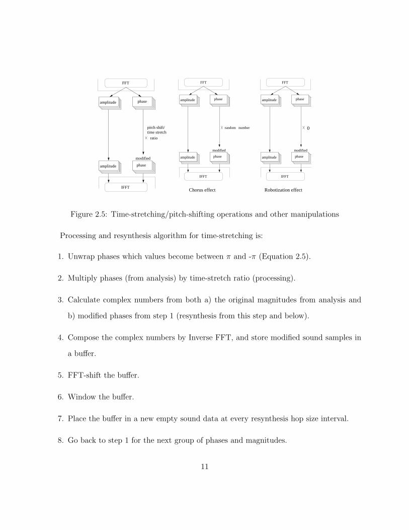
two techniques are very similar; pitch-shifting requires only an additional interpolation stage,

as shown in Figure 2.5. Many other manipulations such as chorus effect and robotization

(Figure 2.5) are also possible (3).

10

amplitude phase

phaseamplitude

modified

FFT

IFFT

pitch shift/time stretch

ratio

amplitude phase

phaseamplitude

modified

FFT

IFFT

Chorus effect

random number

amplitude phase

phaseamplitude

modified

FFT

IFFT

Robotization effect

0

Figure 2.5: Time-stretching/pitch-shifting operations and other manipulations

Processing and resynthesis algorithm for time-stretching is:

1. Unwrap phases which values become between π and -π (Equation 2.5).

2. Multiply phases (from analysis) by time-stretch ratio (processing).

3. Calculate complex numbers from both a) the original magnitudes from analysis and

b) modified phases from step 1 (resynthesis from this step and below).

4. Compose the complex numbers by Inverse FFT, and store modified sound samples in

a buffer.

5. FFT-shift the buffer.

6. Window the buffer.

7. Place the buffer in a new empty sound data at every resynthesis hop size interval.

8. Go back to step 1 for the next group of phases and magnitudes.

11

Processing and resynthesis algorithm for pitch-shifting is:

1. Unwrap phases which values become between π and -π (Equation 2.5).

2. Multiply the phases by pitch-shift ratio (processing).

3. Follow from step 3 to 6 in time-stretching algorithm (resynthesis from this step and

below).

4. Interpolate the sound samples in the buffer.

5. Place the buffer in a new empty sound data at every analysis hop size interval.

6. Go back to step 1.

Because phase is wrapped after 2π (360 degree), phase unwrapping process (3; 22) is nec-

essary to get linearly continuous phase. A more detailed calculation is written in pseudocodes

in Appendix.

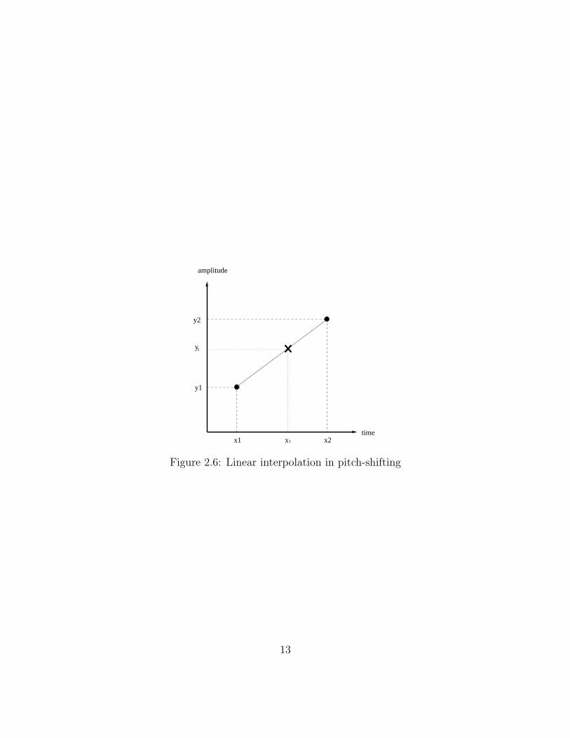
Interpolation (23) is an additional necessary step for pitch-shifting. Up to interpolation,

pitch-shifting steps are followed by time-stretching which results in time-stretched sound

without changing pitches. Then, time-stretched samples need to be resized into the same

size of the original input sound which makes the sound pitch-shifted into an expected amount.

To resize the samples, interpolation is required. In Figure 2.6, (x1, y1) and (x2, y2) are two

samples resulted from time-stretching. xt is the expected time index for the next sample in

pitch-shifting and ytis the expected amplitude value calculated by interpolation:

yt =y2 − y1

x2 − x1

× (xt − x1) + y1 (2.7)

12

x t

ty

time

amplitude

x1 x2

y1

y2

Figure 2.6: Linear interpolation in pitch-shifting

13

Chapter 3

System Overview

setting

parameters

buffer

playback

(offline)

input

audio fileoutput

audio file

visual representations

GUI

vocoder

phase

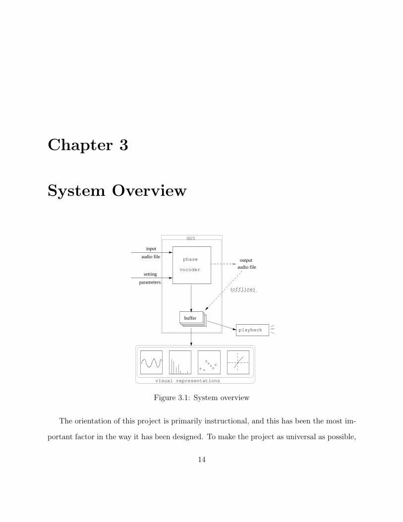
Figure 3.1: System overview

The orientation of this project is primarily instructional, and this has been the most im-

portant factor in the way it has been designed. To make the project as universal as possible,

14

all code is written in ANSI-compliant C, using the gcc compiler (11), and with extensive

comments to clarify details of the implementation. The code has also been modularized as

much as possible. Some of the modules encapsulate a specific type of functionality, such

as data interchange with the sound hardware, and are designed also to be re-used in other

projects. Others, such as the graphic user interface, are dependent and are not designed to

exist on their own. Overall, our program is split into eight basic modules:

Soundcard functions initialization, playing(sending sound data to the soundcard), closing

the soundcard

Sound file handling reading sound file information, writing a sound file

Simple “classic” synthesis waveforms sinusoid, square, sawtooth, triangle waves

Windowing for DSP Hamming, Hanning, triangle, rectangular windows

FFT/complex number functions FFT and IFFT (based on FFTW library (8), getting

complex number, phase and magnitude

Phase vocoder specific functions analysis, processing and resynthesis, fftshift, unwrap-

ping phase(principal argument), interpolation

Graphic user interface(GUI) creating widgets, handling signals, threading

Visual representations waveform, spectrums for amplitude and phase, spectrogram, 3-D

complex number display, magnitude spectrum

We have also tried to use existing open-source code as much as possible. This was partially

to save development time, but also because much of this software is extremely well-tested,

15

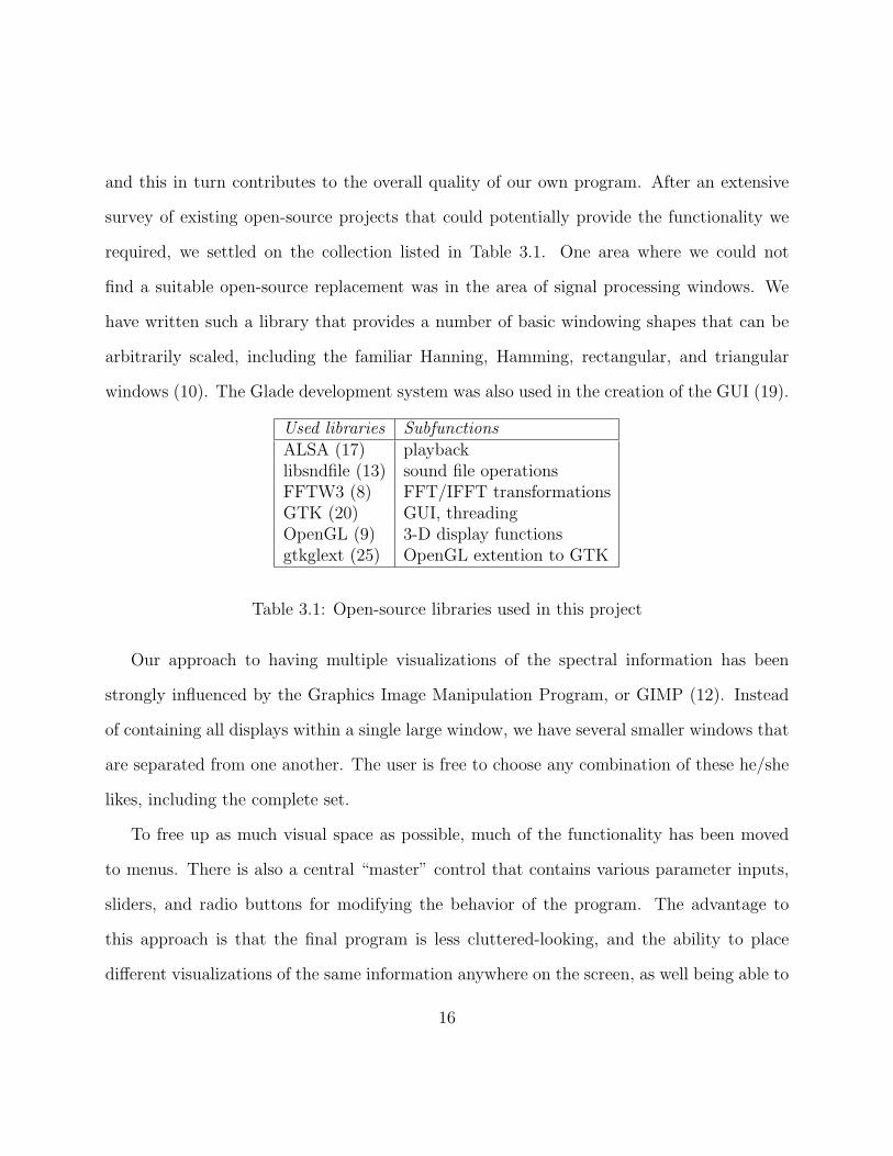
and this in turn contributes to the overall quality of our own program. After an extensive

survey of existing open-source projects that could potentially provide the functionality we

required, we settled on the collection listed in Table 3.1. One area where we could not

find a suitable open-source replacement was in the area of signal processing windows. We

have written such a library that provides a number of basic windowing shapes that can be

arbitrarily scaled, including the familiar Hanning, Hamming, rectangular, and triangular

windows (10). The Glade development system was also used in the creation of the GUI (19).

Used libraries Subfunctions

ALSA (17) playbacklibsndfile (13) sound file operationsFFTW3 (8) FFT/IFFT transformationsGTK (20) GUI, threadingOpenGL (9) 3-D display functionsgtkglext (25) OpenGL extention to GTK

Table 3.1: Open-source libraries used in this project

Our approach to having multiple visualizations of the spectral information has been

strongly influenced by the Graphics Image Manipulation Program, or GIMP (12). Instead

of containing all displays within a single large window, we have several smaller windows that

are separated from one another. The user is free to choose any combination of these he/she

likes, including the complete set.

To free up as much visual space as possible, much of the functionality has been moved

to menus. There is also a central “master” control that contains various parameter inputs,

sliders, and radio buttons for modifying the behavior of the program. The advantage to

this approach is that the final program is less cluttered-looking, and the ability to place

different visualizations of the same information anywhere on the screen, as well being able to

16

simultaneously hear the output, is very useful when trying to understand how the different

ways of viewing this information are connected. This is especially true in the case of beginners

who are trying to understand basic concepts of signal processing.

Figure 3.2: Example of the program in use

After experimenting with several different methods, we finally settled on a fully threaded

implementation to keep all displays synchronized. The overall effect is one of a master control

surrounded by a group of “satellite” windows; an example of the program in operation is

shown in Figure 3.2.

The program has two basic modes of operation.

17

The first is as an offline processor that takes an input sound file and applies global

modifications to the entire sound. Various parameters can be modified, including the FFT

length, window type, hop size, and amount of pitch-shift or time-stretch, and the results

can be saved in various formats. This mode is especially useful for observing the effects of

time-stretching and pitch-shifting, and allows users to create their own modified files.

There is also a second mode of operation where a sound file can be interactively stepped

through on a frame-by-frame basis. In this mode, sound playback is similar to granular

synthesis, with the current frame being repeatedly sounded and overlapped. The advantage

to this is that users can hear the current spectrum, see this information visualized in multiple,

synchronized ways at the same time, and be able to interact with it. This provides a powerful

environment for learning and understanding the connections between the different parts of

the phase vocoder. We know of no other program that presents this information in as clear

and comprehensive a manner. For instance, just being able to observe both the time-domain

and frequency domain information at the same time is enlightening for beginning students

of signal processing. Through direct experience we have this may clarify aspects of the

underlying processes that are difficult to comprehend otherwise. While it is possible to

do similar things with programming environments such as Matlab, the result is slow, non-

interactive, and may require a level of programming skill that many users may not initially

have.

To test some of our initial modules, and to learn to understand the GTK toolkit better,

we initially created two “testing” projects that are included with the main program. The first

was a simple tone generator that creates and plays different waveform sounds. Additionally, a

granular synthesizer that does offline synthesis using real sounds was also implemented. The

18

granular synthesizer was especially useful to work out, as it shares the basic ideas of frame-

by-frame processing of a sound file (but without the FFT processing). These additional

programs serve as good examples of basic sound programming in the linux environment and

may be of use to some users.

19

Chapter 4

Visualizations

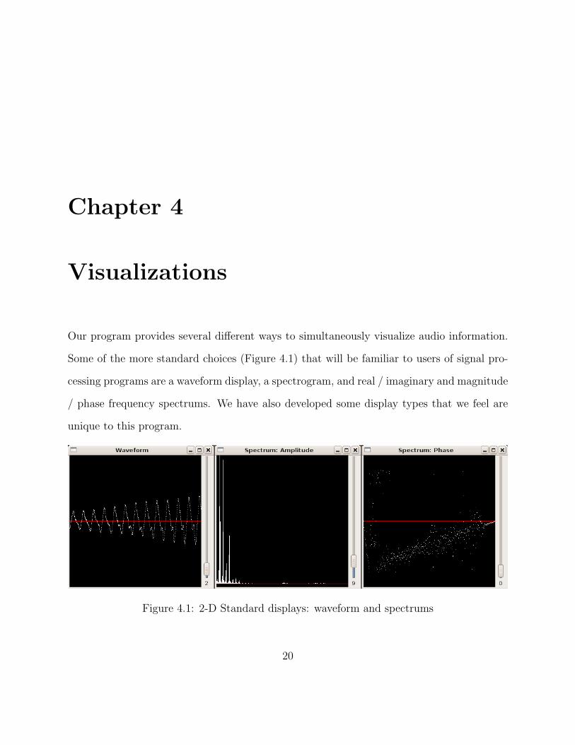
Our program provides several different ways to simultaneously visualize audio information.

Some of the more standard choices (Figure 4.1) that will be familiar to users of signal pro-

cessing programs are a waveform display, a spectrogram, and real / imaginary and magnitude

/ phase frequency spectrums. We have also developed some display types that we feel are

unique to this program.

Figure 4.1: 2-D Standard displays: waveform and spectrums

20

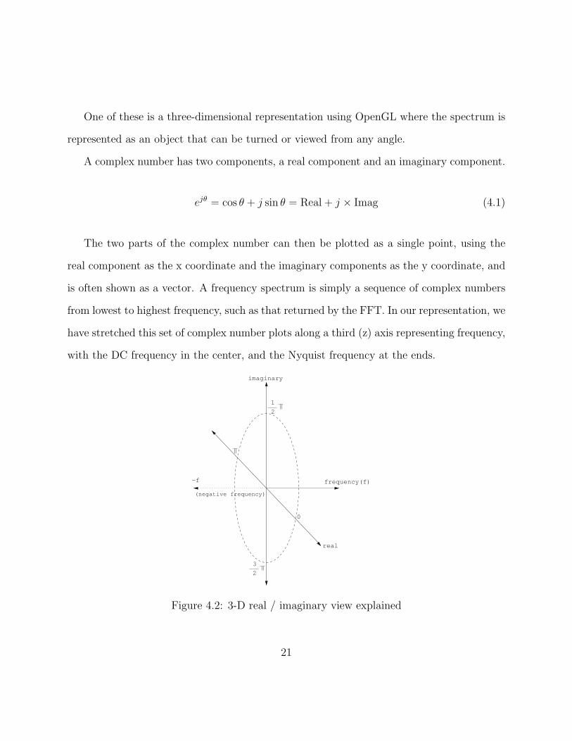
One of these is a three-dimensional representation using OpenGL where the spectrum is

represented as an object that can be turned or viewed from any angle.

A complex number has two components, a real component and an imaginary component.

ejθ = cos θ + j sin θ = Real + j × Imag (4.1)

The two parts of the complex number can then be plotted as a single point, using the

real component as the x coordinate and the imaginary components as the y coordinate, and

is often shown as a vector. A frequency spectrum is simply a sequence of complex numbers

from lowest to highest frequency, such as that returned by the FFT. In our representation, we

have stretched this set of complex number plots along a third (z) axis representing frequency,

with the DC frequency in the center, and the Nyquist frequency at the ends.

real

frequency(f)

imaginary

2

1

−f

2

3

0

(negative frequency)

Figure 4.2: 3-D real / imaginary view explained

21

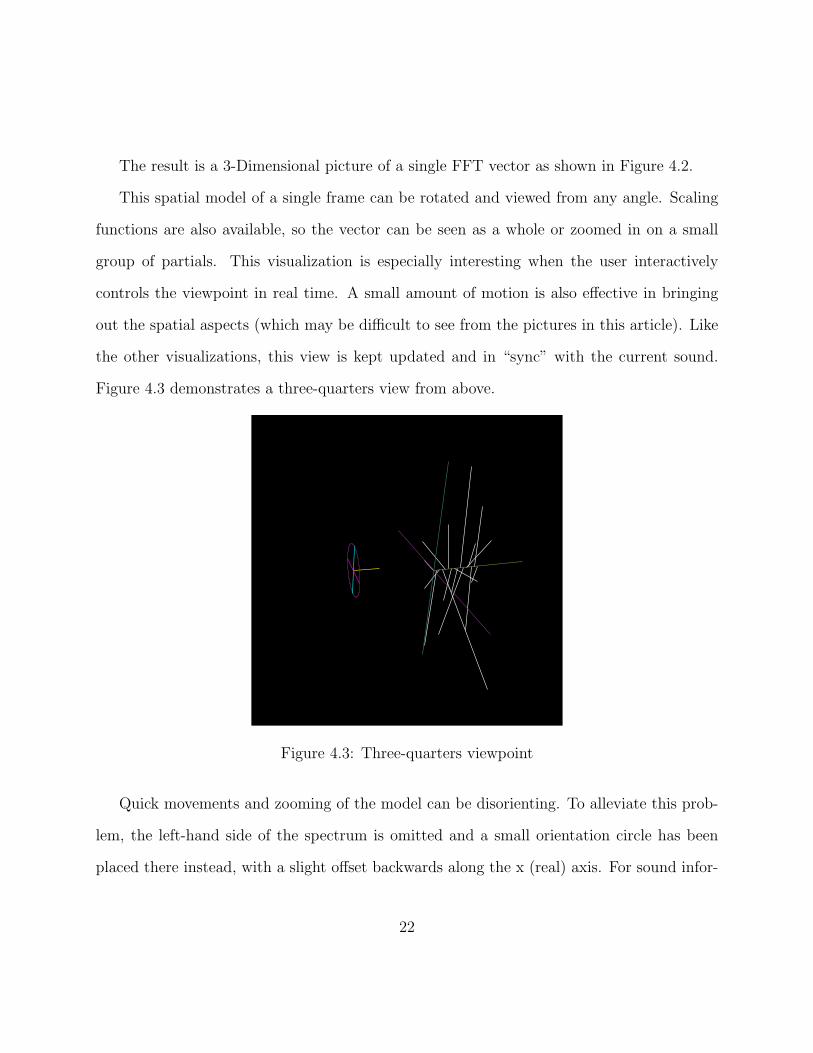
The result is a 3-Dimensional picture of a single FFT vector as shown in Figure 4.2.

This spatial model of a single frame can be rotated and viewed from any angle. Scaling

functions are also available, so the vector can be seen as a whole or zoomed in on a small

group of partials. This visualization is especially interesting when the user interactively

controls the viewpoint in real time. A small amount of motion is also effective in bringing

out the spatial aspects (which may be difficult to see from the pictures in this article). Like

the other visualizations, this view is kept updated and in “sync” with the current sound.

Figure 4.3 demonstrates a three-quarters view from above.

Figure 4.3: Three-quarters viewpoint

Quick movements and zooming of the model can be disorienting. To alleviate this prob-

lem, the left-hand side of the spectrum is omitted and a small orientation circle has been

placed there instead, with a slight offset backwards along the x (real) axis. For sound infor-

22

mation, the left hand side is a mirror of the right-hand side (with a shift of π in the y axis)

and can be safely omitted, as is customary in many frequency-domain displays.

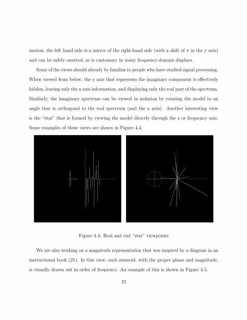
Some of the views should already be familiar to people who have studied signal processing.

When viewed from below, the y axis that represents the imaginary component is effectively

hidden, leaving only the x axis information, and displaying only the real part of the spectrum.

Similarly, the imaginary spectrum can be viewed in isolation by rotating the model to an

angle that is orthogonal to the real spectrum (and the x axis). Another interesting view

is the “star” that is formed by viewing the model directly through the z or frequency axis.

Some examples of these views are shown in Figure 4.4.

Figure 4.4: Real and end “star” viewpoints

We are also working on a magnitude representation that was inspired by a diagram in an

instructional book (21). In this view, each sinusoid, with the proper phase and magnitude,

is visually drawn out in order of frequency. An example of this is shown in Figure 4.5.

23

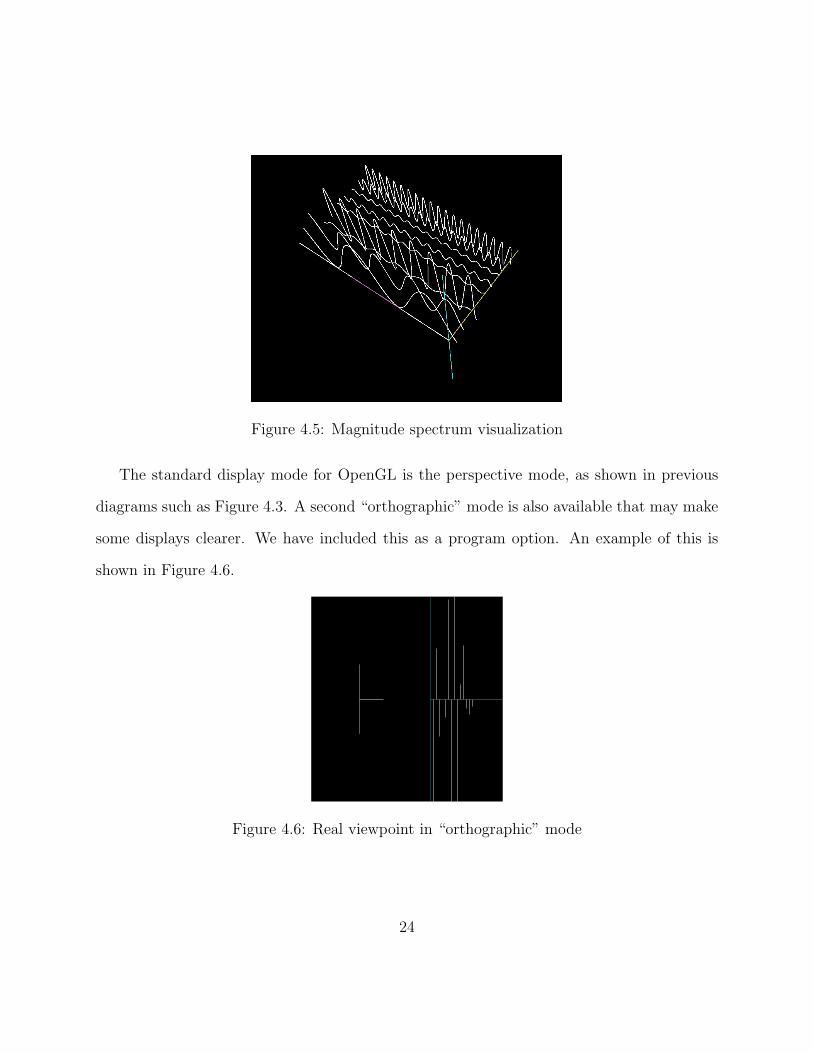
Figure 4.5: Magnitude spectrum visualization

The standard display mode for OpenGL is the perspective mode, as shown in previous

diagrams such as Figure 4.3. A second “orthographic” mode is also available that may make

some displays clearer. We have included this as a program option. An example of this is

shown in Figure 4.6.

Figure 4.6: Real viewpoint in “orthographic” mode

24

Chapter 5

Results and Discussion

We have been using a Debian Linux platform and C programming language. They are

good choices because of their greater control of audio elements. C programming in Linux

also provides more power because of its portability to programs to other platforms such as

Microsoft Windows or Macintosh. Also, open-source libraries that the Linux world shares

are important resources for our application development. Personally, it has been a good

opportunity for me to expose to computer hardware by working at Linux system.

While implementating the phase vocoder, I realized more and more that explanations

about processing stage between analysis and resynthesis in most tutorials are often not

sufficient. Without clear idea about how processing part works, it is difficult to design and

implement the phase vocoder. Even, distributed example codes written in C and Matlab are

not clear even besides each language’s unique style of programming. Debugging in digital

audio related programming is also complicated because the outcomes are complex numbers

and floating points. Because of these difficulties, we created short audio sound such as ticks

25

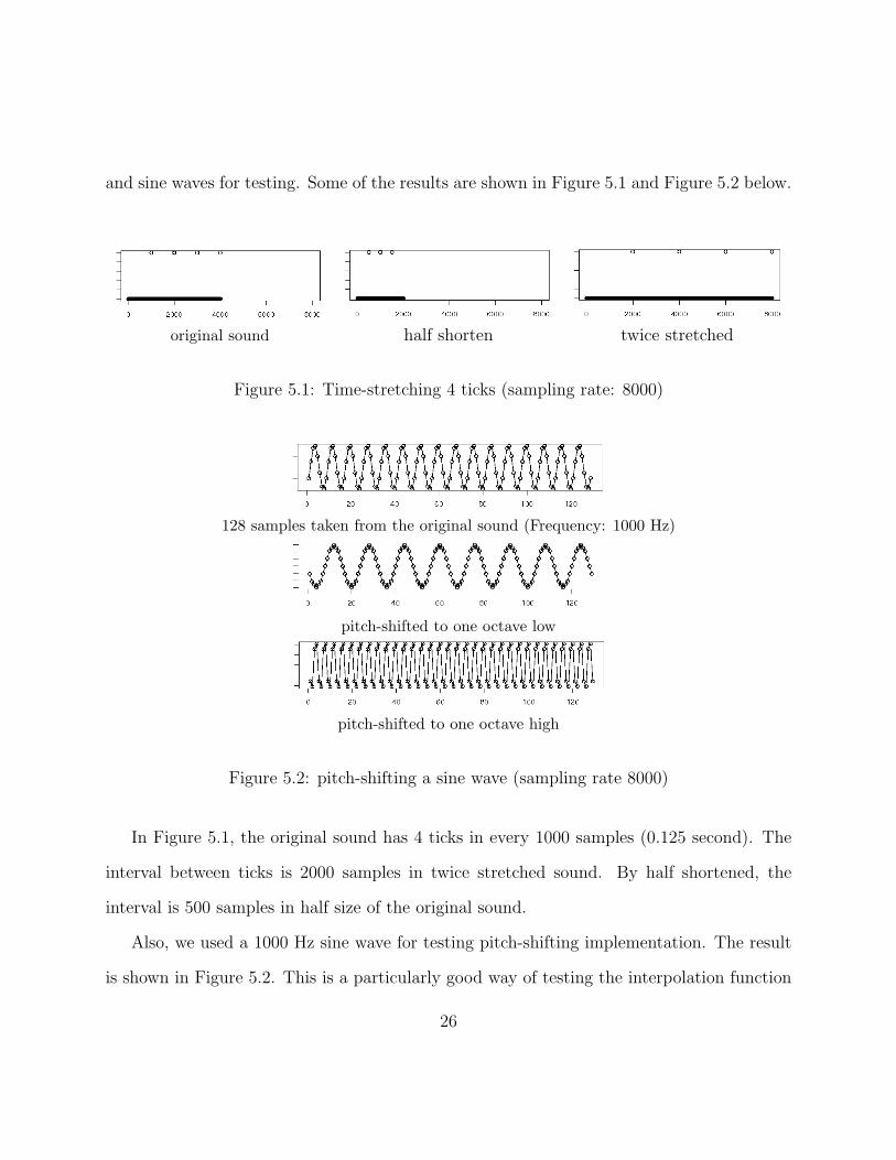
and sine waves for testing. Some of the results are shown in Figure 5.1 and Figure 5.2 below.

original sound half shorten twice stretched

Figure 5.1: Time-stretching 4 ticks (sampling rate: 8000)

128 samples taken from the original sound (Frequency: 1000 Hz)

pitch-shifted to one octave low

pitch-shifted to one octave high

Figure 5.2: pitch-shifting a sine wave (sampling rate 8000)

In Figure 5.1, the original sound has 4 ticks in every 1000 samples (0.125 second). The

interval between ticks is 2000 samples in twice stretched sound. By half shortened, the

interval is 500 samples in half size of the original sound.

Also, we used a 1000 Hz sine wave for testing pitch-shifting implementation. The result

is shown in Figure 5.2. This is a particularly good way of testing the interpolation function

26

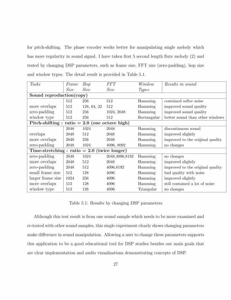
for pitch-shifting. The phase vocoder works better for manipulating single melody which

has more regularity in sound signal. I have taken first 5 second length flute melody (2) and

tested by changing DSP parameters, such as frame size, FFT size (zero-padding), hop size

and window types. The detail result is provided in Table 5.1.

Tasks Frame Hop FFT Window Results in sound

Size Size Size Types

Sound reproduction(copy)512 256 512 Hamming contained softer noise

more overlaps 512 128, 64, 32 512 Hamming improved sound quality

zero-padding 512 256 1024, 2048 Hamming improved sound quality

window type 512 256 512 Rectangular better sound than other windows

Pitch-shifting : ratio = 2.0 (one octave high)2048 1024 2048 Hamming discontinuous sound

overlaps 2048 512 2048 Hamming improved slightly

more overlaps 2048 256 2048 Hamming improved to the original quality

zero-padding 2048 1024 4096, 8092 Hamming no changes

Time-stretching : ratio = 2.0 (twice longer)zero-padding 2048 1024 2048,4096,8192 Hamming no changes

more overlaps 2048 512 2048 Hamming improved slightly

zero-padding 2048 512 4096,8192 Hamming improved to the original quality

small frame size 512 128 4096 Hamming bad quality with noise

larger frame size 1024 256 4096 Hamming improved slightly

more overlaps 512 128 4096 Hamming still contained a lot of noise

window type 512 128 4096 Triangular no changes

Table 5.1: Results by changing DSP parameters

Although this test result is from one sound sample which needs to be more examined and

re-tested with other sound samples, this single experiment clearly shows changing parameters

make difference in sound manipulation. Allowing a user to change these parameters supports

this application to be a good educational tool for DSP studies besides our main goals that

are clear implementation and audio visualizations demonstrating concepts of DSP.

27

In the later stage of this project, we have been exposed more to OpenGL libraries which

are powerful and flexible for visualizations. The GTK library is sufficient for GUI and simple

2-D displays, but not flexible enough to handle window signals for complicated pictures such

as spectrogram or 3-D visualization. Using the OpenGL library has improved the visualiza-

tions and we are still adopting more functions from OpenGL. This is further explained in

the next chapter.

28

Chapter 6

Future work

The phase vocoder used here works quite well and is an excellent basis for future expansion.

The main “effects” that we have incorporated so far are the time stretching and pitch shifting

operations. A variety of additional effects are possible with the phase vocoder (26), and we

would like to include more of these.

Currently we are using the standard GTK widgets such as sliders, radio buttons, etc.

There are some places where widgets that are specific to sound operations are desirable.

For instance, selecting window shapes, hop sizes, or zero padding amounts could be done by

dragging elements of a picture. We have not explored designing custom widgets for sound

control yet, but intend to explore this in the future. There are also some other common

displays such as phaseograms and waterfall-style spectrogram plots that we would like to

incorporate into the program.

Our system at present is primarily oriented towards visualization of various aspects of the

phase vocoding process. We believe that the current visualization system can be extended

29

to an editing system. This would be especially effective with the 3-D OpenGL display parts,

where particular partials and harmonic structure could be zoomed in on and manipulated

directly using various functions, or even with the mouse. We are currently experimenting

with incorporating this. A further extension would be to incorporate some sort of system that

displays the three-dimensional information in a three-dimensional space, such as a virtual

reality system using display goggles, or perhaps even something tactile. The idea of actually

being able to edit sound using just one’s hands is exciting, and well within the potential of

this project.

30

Bibliography

[1] S. M. Bernsee. Time stretching and pitch shifting of audio signals - an overview, 2007.Retrieved April 29, 2007 from http://www.bernsee.com.

[2] C. Bolling and J. Rampal. Suite for flute and jazz piano trio no.1 fugace, 1993. MilanRecords.

[3] A. De Goetzen, N. Bernardini, and D. Arfib. Traditional(?) implementations of a phase-vocoder: The tricks of the trade. In Proceedings of Digital Audio Effects Conference,pages 37–44, 2000.

[4] M. Dolson. The phase vocoder: a tutorial. Computer Music Journal, 10(4):14–27, 1986.

[5] H. Dudley. The vocoder. Bell Laboratories Record, 17:122–6, 1939.

[6] D. Ellis. A phase vocoder in matlab, 2007. Retrieved April 29, 2007 from http:

//labrosa.ee.columbia.edu/matlab/pvoc/.

[7] J. L. Flanagan and R. M. Golden. Phase vocoder. Bell System Technical Journal,45:1493–509, 1966.

[8] M. Frigo and S. G. Johnson. FFTW, 2007. http://www.fftw.org/.

[9] Khronos Group. OpenGL, 2006. http://www.opengl.org.

[10] F. Harris. On the use of windows for harmonic analysis with the discrete fourier trans-form. Proceedings of the IEEE, 66(1):51–83, 1978.

[11] Free Software Foundataion Inc. GNU gcc, 2007. http://gcc.gnu.org.

[12] S. Kimball and P. Mattis. GNU Image Manipulation Program, 2007. http://www.

gimp.org.

[13] E. Lopo. libsndfile, 2006. http://www.mega-nerd.com/libsndfile.

31

[14] R. G. Lyons. Understanding Digital Signal Processing. Prentice Hall, 2004.

[15] F. R. Moorer. Elements of Computer Music. Prentice Hall, 1990.

[16] J. A. Moorer. The use of the phase vocoder in computer music applications. Journal of

the Audio Engineering Society, 1–2(26):42–5, 1978.

[17] ALSA Project. Advanced Linux Sound Architecture, 2005. http://www.

alsa-project.org.

[18] CRAN R Project. R, 2007. http://cran.r-project.org/.

[19] GNOME Project. Glade, 2007. Retrieved on April 29, 2007 from http://glade.gnome.

org/.

[20] GNU Project. The Gimp Tool Kit, 2006. http://www.gtk.org.

[21] R. W. Ramirez. The FFT: fundamentals and concepts. Prentice-Hall, Englewood Cliffs,New Jersey, 1985.

[22] C. Roads. The Computer Music Tutorial. The MIT Press, 1996.

[23] J. O. Simth. Physical Audio Signal Processing: for Virtual Musical Instruments and

Digital Audio Effects. Center for Computer Research in Music and Acoustics (CCRMA),Stanford University, 2006.

[24] S. W. Smith. The Scientist and Engineer’s Guide to Digital Signal Processing. CaliforniaTechnical Publisher, 1997.

[25] N. Yasufuku and T. Shead. gtkglext, 2007. http://www.k-3d.org/gtkglext/Main

Page.

[26] U. Zolzer and X. Amatriain, editors. DAFX: digital audio effects. Wiley, New York,USA, 2002.

32

Appendix A

Phase vocoder pseudocodes

A.1 Common variables

framesize

fftsize

analysis_hopsize

resynthesis_hopsize

number_of_frame = input_sound_size/analysis_hopsize

magnitude[number_of_frame][fftsize]

phase[number_of_frame][fftsize]

buffer[fftsize]

window_type

windowbuffer[framesize]

A.2 Analysis

Input: input_sound_info, fftsize, window_type,

framesize, analysis_hopsize, number_of_frame

Output: magnitude, phase

-----------------------------------------------------------------------------

input_index = 0;

fft_complex_number[fftsize];//has both real and imaginary parts

windowbuffer = window(windowtype, framesize);

33

for(i=0; i<number_of_frame; i++){

for(j=0; j<framesize; j++){

buffer[j] = input_sound[input_index + j]*windowbuffer[j];

}

fftshift(buffer);

fft(buffer, fft_complex_number);

get_magnitude(magnitude[i][], fft_complex_number);

get_phase(phase[i][], fft_complex_number);

input_index += analysis_hop;

}

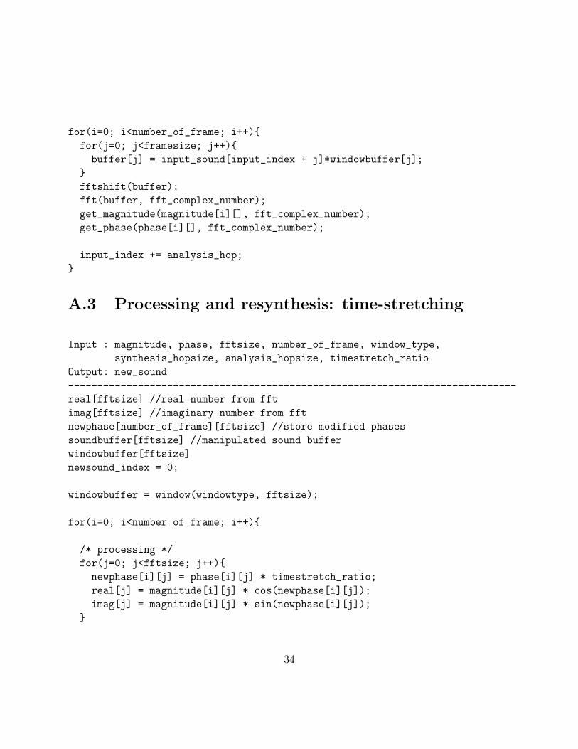
A.3 Processing and resynthesis: time-stretching

Input : magnitude, phase, fftsize, number_of_frame, window_type,

synthesis_hopsize, analysis_hopsize, timestretch_ratio

Output: new_sound

-----------------------------------------------------------------------------

real[fftsize] //real number from fft

imag[fftsize] //imaginary number from fft

newphase[number_of_frame][fftsize] //store modified phases

soundbuffer[fftsize] //manipulated sound buffer

windowbuffer[fftsize]

newsound_index = 0;

windowbuffer = window(windowtype, fftsize);


/* processing */

for(j=0; j<fftsize; j++){

newphase[i][j] = phase[i][j] * timestretch_ratio;

real[j] = magnitude[i][j] * cos(newphase[i][j]);

imag[j] = magnitude[i][j] * sin(newphase[i][j]);

}

34

/* resyntehsis */

ifft(real, imag, soundbuffer); //soundbuffer has time domain sound data

fftshift(soundbuffer);


new_sound[newsound_index + j] = new_sound[newsound_index + j]

+ soundbuffer[j] * winbuffer[j];

}

newsound_index += synthesis_hopsize;

}

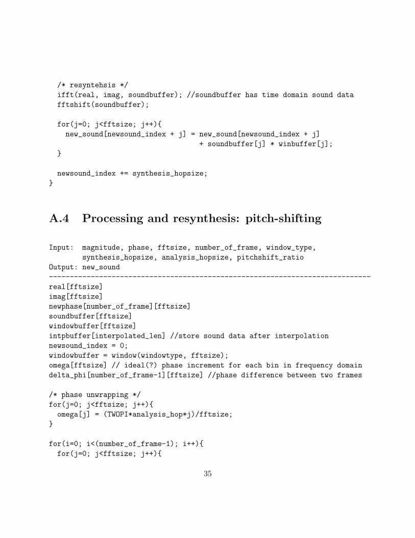
A.4 Processing and resynthesis: pitch-shifting

Input: magnitude, phase, fftsize, number_of_frame, window_type,

synthesis_hopsize, analysis_hopsize, pitchshift_ratio

Output: new_sound

-----------------------------------------------------------------------------

real[fftsize]

imag[fftsize]

newphase[number_of_frame][fftsize]

soundbuffer[fftsize]

windowbuffer[fftsize]

intpbuffer[interpolated_len] //store sound data after interpolation

newsound_index = 0;

windowbuffer = window(windowtype, fftsize);

omega[fftsize] // ideal(?) phase increment for each bin in frequency domain

delta_phi[number_of_frame-1][fftsize] //phase difference between two frames

/* phase unwrapping */


omega[j] = (TWOPI*analysis_hop*j)/fftsize;

}

for(i=0; i<(number_of_frame-1); i++){


35

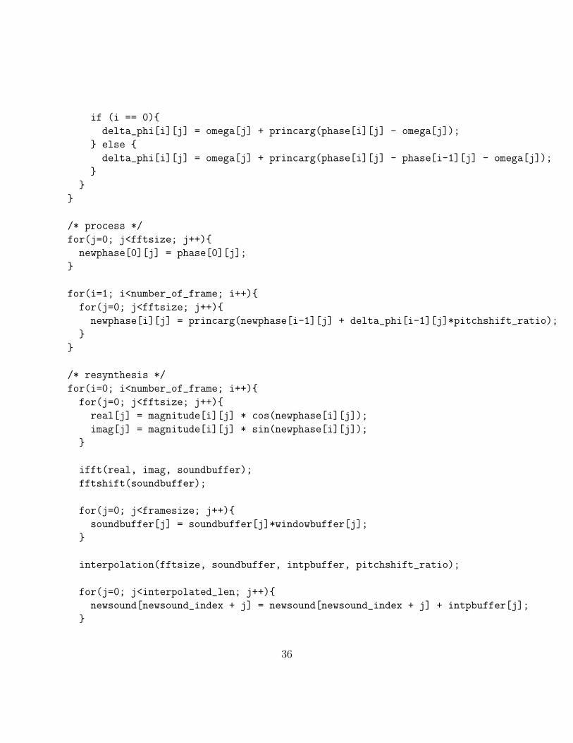
if (i == 0){

delta_phi[i][j] = omega[j] + princarg(phase[i][j] - omega[j]);

} else {

delta_phi[i][j] = omega[j] + princarg(phase[i][j] - phase[i-1][j] - omega[j]);

}

}

}

/* process */


newphase[0][j] = phase[0][j];

}



newphase[i][j] = princarg(newphase[i-1][j] + delta_phi[i-1][j]*pitchshift_ratio);

}

}

/* resynthesis */



real[j] = magnitude[i][j] * cos(newphase[i][j]);

imag[j] = magnitude[i][j] * sin(newphase[i][j]);

}

ifft(real, imag, soundbuffer);

fftshift(soundbuffer);

for(j=0; j<framesize; j++){

soundbuffer[j] = soundbuffer[j]*windowbuffer[j];

}

interpolation(fftsize, soundbuffer, intpbuffer, pitchshift_ratio);

for(j=0; j<interpolated_len; j++){

newsound[newsound_index + j] = newsound[newsound_index + j] + intpbuffer[j];

}

36

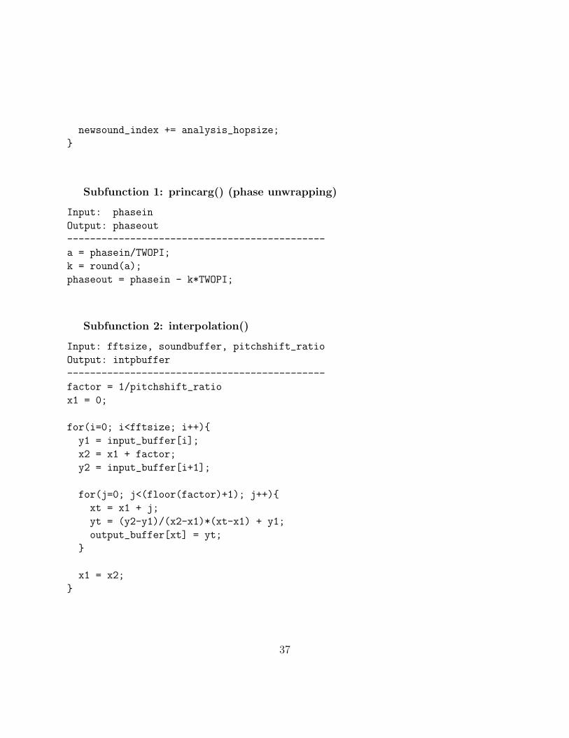
newsound_index += analysis_hopsize;

}

Subfunction 1: princarg() (phase unwrapping)

Input: phasein

Output: phaseout

---------------------------------------------

a = phasein/TWOPI;

k = round(a);

phaseout = phasein - k*TWOPI;

Subfunction 2: interpolation()

Input: fftsize, soundbuffer, pitchshift_ratio

Output: intpbuffer

---------------------------------------------

factor = 1/pitchshift_ratio

x1 = 0;

for(i=0; i<fftsize; i++){

y1 = input_buffer[i];

x2 = x1 + factor;

y2 = input_buffer[i+1];

for(j=0; j<(floor(factor)+1); j++){

xt = x1 + j;

yt = (y2-y1)/(x2-x1)*(xt-x1) + y1;

output_buffer[xt] = yt;

}

x1 = x2;

}

37

Documents

An Open-Source Phase Vocoder with Some - Music Informatics