An Online Mapping Algorithmfor Teams of Mobile Robots

Sebastian Thrun

October 2000CMU-CS-00-167

School of Computer ScienceCarnegie Mellon University

Pittsburgh, PA 15213

Abstract

We propose a new probabilistic algorithm for online mapping of unknown environmentswith teams of robots. At the core of the algorithm is a technique that combines fast max-imum likelihood map growing with a Monte Carlo localizer that uses particle representa-tions. The combination of both yields an online algorithm that can cope with large odo-metric errors typically found when mapping an environment with cycles. The algorithmcan be implemented distributedly on multiple robot platforms, enabling a team of robots tocooperatively generate a single map of their environment. Finally, an extension is describedfor acquiring three-dimensional maps, which capture the structure and visual appearance ofindoor environments in 3D.

This research is sponsored by the National Science Foundation (and CAREER grant number IIS-9876136and regular grant number IIS-9877033), and by DARPA-ATO via TACOM (contract number DAAE07-98-C-L032), which is gratefully acknowledged. The views and conclusions contained in this document are those ofthe author and should not be interpreted as necessarily representing official policies or endorsements, eitherexpressed or implied, of the United States Government or any of the sponsoring institutions.

Keywords: Bayes filters, particle filters, mobile robots, multi-robot systems, proba-bilistic robotics, robotic exploration, robot mapping

1 Introduction

The problem of robot mapping has received considerable attention over the past few years.Mapping is the problem of generating models of robot environments from sensor data. Tomap an environment, a robot has to cope with two types of sensor noise: Noise in percep-tion (e.g., range measurements), and noise in odometry (e.g., wheel encoders). Because ofthe latter, the problem of mapping creates an inherent localization problem, which is theproblem of determining the location of a robot relative to its own map. Because of this, themapping problem is often referred to as theconcurrent mapping and localization problem,thesimultaneous localization and mapping problem, or simplySLAM.

The importance of the problem is due to the fact that many successful mobile robotsystems require a map for their operation. Examples include the Helpmate hospital deliveryrobot [30], Simmons’s Xavier robot [60], and various museum tour-guide robots [2, 25, 48,65]. Consequently, over the last decade, there has been a flurry of work on map buildingfor mobile robots (see e.g., [7, 36, 54, 67]). Some approaches seek to devise abstract,topological descriptions of robot environments [1, 8, 33, 42], whereas others generate moredetailed, metric maps [7, 15, 22, 39, 44]. Naturally, the problem of mapping lends itselfnicely to multi-robot solutions, where multiple robots collaborate and jointly explore anunknown environment.

In this paper, we will be interested in the problem of building detailed metric mapsonline, while the robot is in motion. The online characteristic is important for a range ofpractical problems, such as the robot exploration problem, where mapping is constantlyinterleaved with decision making as to where to move next. This paper addresses threeimportant open problems in online mapping: the problem of mapping cyclic environments,the problem of generating maps with multiple robots, and the problem of generating three-dimensional maps of building interiors.

Environments with cycles are particularly difficult to map. When closing a cycle, therobot might have accrued a large odometry error. Past solutions, which are discussed indepth towards the end of this paper, either have to resort to highly restrictive assumptionson the nature of the sensor data, or require extensive batch computation to generate a mapof cyclic environments. The problem is even more challenging when multiple robots jointlyacquire a map. Scalable solutions must perform the computation distirbutedly.

The core of this paper is a statistical framework that combines an incremental maximumlikelihood estimator with a posterior pose estimator. More specifically, maps are generatedonline by finding the most likely continuation of the previous maps under the most recentsensor measurement. However, while online, such a methodology is prone to failure whenmapping a cycle. This is because when mapping a cycle, the error in pose estimation mightbe very large, requiring a backwards-correction of past estimates. To overcome this prob-lem, we propose a second estimator that estimates the residual uncertainty in the robot’spose. When closing the cycle, this estimate is used to determine the robot’s pose relativeto its own map, and to correct pose estimates backwards in time to resolve inconsistencies.The resulting mapping algorithm is shown to perform favorably in a range of challenging

1

mapping problems. Moreover, it is easily extended into a modular multi-robot mappingapproach, where multiple robots integrate sensor measurements into a single, global map.

In addition, we describe an extension of the mapping algorithm that generates 3D maps,reflecting the structural and optical appearance of a building’s interior. 3D maps are gen-erated from a a panoramic camera and a laser range sensor mounted perpendicular to therobot’s motion direction. They are represented in a standard virtual reality format (VRML),thereby enabling people to interactively ‘fly through’ an environment from a remote loca-tion.

The paper is organized as follows. We begin with introducing the basic statistical frame-work, which encompasses virtually all major probabilistic mapping algorithms in the liter-ature. From there, we develop the specific set of estimators, making explicit the variousassumptions and approximations necessary to obtain a working online algorithm. The algo-rithm is then extended into a scalable multi-robot mapping algorithm, which under specificinitial conditions is shown to enable teams of robots to buildaccurate maps. Finally, wedescribe our approach to generating maps in 3D and show results of mapping a corridorsegment in our university building. The paper is concluded with a discussion of limitations,related work, and research opportunities that arise from this work.

2 Mapping as Posterior Estimation

2.1 Bayes Filters

Bayes filtersare at the core of the algorithm presented here. They comprise a popular classof Bayesian estimation algorithms that are in widespread use of robotics and engineering.Special versions of Bayes filters are known as Kalman filters [28], hidden Markov mod-els [53, 52], and dynamic belief networks [9, 31, 56]. The classical probabilistic occupancygrid mapping algorithm [15, 44] is also a (binary) Bayes filter.

Bayes filtering addresses the problem of estimating an unknown quantity from sensormeasurements. In its most general form, it can estimate the state of a time-varying (dy-namic) system, such as a mobile robot. Let us denote the state of the environment byx;the state at timex will be denotedxt. Furthermore, let us denote measurements byz, andthe measurement at timet by zt. In time-varying systems (and in robotic in particular),the change of state is often a function of the controls. Controls will be denoted byu. Thecontrol at timet, ut determines the change of state in the time interval(t; t+ 1]. The set ofall measurements and controls will be referred asdataand denoted byd:

dt = fz0; u0; z1; u1; : : : ; ztg (1)

Without loss of generality, we assume that controls and measurements are alternated. Fol-lowing standard notation, we adopt the subscriptt to denote to an event at timet, and thesuperscriptt to denote to the set of all events up to and including timet.

The Bayes filter calculates the posterior probabilityp(xtjdt) of the statext conditioned

on the data leading up to timet. It does so recursively, i.e., the estimatep(xtjdt) is cal-

2

culated from the previous posteriorp(xt�1jdt�1) using only the most recent control,ut�1,

and measurement,zt. Once processed, data can be discarded. Hence the time required tocalculatep(xtjdt) does not depend on the size of the data set. This online property makesBayes filters well-suited for a range of robotic estimation problem, such as the concurrentmapping and localization problem discussed here.

The recursive update equation of the Bayes filter is as follows:

p(xtjdt) = p(ztjxt)

Zp(xtjut�1; xt�1) p(xt�1jd

t�1) dxt�1 (2)

Thus, the desired posteriorp(xtjdt) is obtained from the estimate one time step earlier,p(xt�1jd

t�1), after incorporating the controlut�1 and the measurementzt. The nature ofthe conditional probabilitiesp(ztjxt) andp(xtjut�1; xt�1), which play an essential role inthis recursive estimator, are discussed in a separate section further below.

Bayes filters owe their validity a specific assumption concerning the nature of the envi-ronment, called theMarkov assumption. The Markov assumption states that given knowl-edge of the current state, the future is independent of the past. In particular, this impliesthat the posterior estimatep(xtjdt) is a sufficient statistics of past data, with regards to pre-diction. This assumption is true for worlds in whichx is the only state that affects multiplemeasurements. In static environments, the state comprises the robot pose and the shape ofthe environment itself. This suggests that the Markov assumption holds true in the concur-rent mapping and localization problem. Clearly, in crowded environments the assumptionis violated unless people are included in the statex. This case is therefore not addressed inthe framework presented here.

To derive Bayes filters, we notice that the desired posterior can be written as

p(xtjdt) = p(xtjzt; ut�1; d

t�1) (3)

Applying Bayes rule leads to

= � p(ztjxt; ut�1; dt�1) p(xtjut�1; d

t�1) (4)

where� is a normalizer. The Markov assumption allows us to simplify the termp(ztjxt; ut�1; dt�1),

which leads to the more convenient form

= � p(ztjxt) p(xtjut�1; dt�1) (5)

Next, we integrate the second term over the previous statext�1, which gives us

= � p(ztjxt)

Zp(xtjut�1; d

t�1; xt�1) p(xt�1jut�1; dt�1) dxt�1 (6)

Exploiting the Markov assumption once again, we obtain the simplified form

= � p(ztjxt)

Zp(xtjut�1; xt�1) p(xt�1jd

t�1) dxt�1 (7)

which completes the derivation of the Bayes filter.

3

2.2 Concurrent Mapping and Localization

In concurrent mapping and localization, the statex comprises the (unknown) map of theenvironment and the pose of the robot. Let us denote the map bym and the pose bys. Thenwe have

x = hm; si (8)

This gives rise to the following filter, which describes the problem of concurrent mappingand localization in Bayesian terminology:

p(st; mtjdt) = p(ztjst; mt)

Z Zp(st; mtjut�1; st�1; mt�1)

p(st�1; mt�1jdt�1) dst�1 dmt�1 (9)

This equation is obtained by substituting (8) into (2).If the world does not change over time, which is commonly assumed in the liter-

ature on concurrent mapping and localization, we havemt = mt�1. Hence, the termp(st; mtjut�1; st�1; mt�1) is only non-zero ifmt = mt�1, and the integration can be omit-ted:

= p(ztjst; mt)

Zp(stjut�1; st�1; mt�1) p(st�1; mt�1jd

t�1) dst�1 (10)

Stripping the mapm of its time index leads to

p(st; mjdt) = p(ztjst; m)

Zp(stjut�1; st�1; m) p(st�1; mjd

t�1) dst�1 (11)

It is also common, but not essential, to assume that the effect of robot motion does notdepend on the mapm. This leads to the recursive estimator:

p(st; mjdt) = p(ztjst; m)

Zp(stjut�1; st�1) p(st�1; mjd

t�1) dst�1 (12)

This important equation is at the heart of all state-of-the-art concurrent mapping and local-ization algorithms. Virtually all competitive algorithms can be derived from this equation.

Unfortunately, the computation of the joint posterior over poses and maps is intractablein the context of concurrent mapping and localization, due to the high dimensionality of thespace of all maps. Hence, all existing approaches make further restrictive assumptions. Forexample, the SLAM family of approaches [12, 36, 47, 63] assumes Gaussian-distributednoise and local-linear perception and motion models. Under these assumptions, the poste-rior can be computed using the extended Kalman filter, transforming the exponentially hardproblem into one that scales quadratically in the size of the environment [46, 47]. However,the Gaussian noise assumption has important ramifications in practice. Among others, it re-quires that sensor measurements can be uniquely associated with objects in the real world,a problem commonly referred to asdata association.

The data association problem is overcome by a complimentary family of approaches,know asEM [59, 67] (based on Dempster’sexpectation maximizationalgorithm [11]). This

4

(a) (b)

Figure 1: The motion model: Posterior distributions of the robot’s pose upon executing the controlillustratedby the solid line. The darker a pose, the more likely it is. Poses are projected into 2D, ignoring the robot’sheading direction.

approach generates a map by likelihood maximization, treating the robot poses as latentvariables. For a fixed data set, it alternates a mapping and a localization step, which aftermultiple iterations generates a map that locally maximizes the likelihood for unknown dataassociation. Unfortunately, EM is not an online algorithm, hence is inapplicable to problemssuch as mobile robot exploration.

2.3 Probabilistic Models

To implement the recursive update equation (12), we need three quantities: a distributionp(s0; m) for initializing the filter, and the conditional distributionsp(stjut�1; st�1) andp(ztjst; m). The latter distributions are often referred to asmotion modelandmeasurementmodel, respectively, since they physically model robot’s motion and its sensors.

The initial distribution in mapping is straightforward. Without loss of generality, theposes0 is defined to be the origin of the coordinate system with a heading direction of0

degrees, that is,s0 = h0; 0; 0i. The mapm is initialized with a uniform prior.The motion model,p(stjut�1; st�1), specifies the probability that the robot’s pose isst

given that it executed the controlut�1 at timet�1. Thus, the motion model is a probabilisticgeneralization of mobile robot kinematics. Classical kinematics specifies where one wouldexpect a robot to see if its control and its motion were perfect. In practice, physical robotsoften suffer from drift an slippage, which induce deviations from the expected pose that aredifficult to predict. Hence, the posest is best modeled by a probability distribution overpossible poses that the robot might attain after executingut�1 in st�1.

In our implementation, we assume that the robot experiences translational and rotationalerror. For a small motion segment (e.g., the distance a robot traverses in .25 seconds), weassume that these errors can be modeled by two independent Gaussian noise variables,which are added to the commanded translation and rotation. Figure 1 shows two examplesof the probabilistic motion modelp(stjut�1; st�1). In both cases, the robot’s pose prior toexecuting the control is shown on the left. The robot is then commanded to follow a straight-

5

(a)

(b)

Figure 2: (a) Laser range scan projected into an occupancy grid map. (b) Probabilistic measurement model foran example range scan, which assigns likelihood in proportion to how close to the scan a non-occluded objectwas observed.

line motion as indicated. The posterior pose after executing the respective motion commandis shown in Figure 1, as indicated by the grayly shaded area. The darker a pose, the morelikely it is. Obviously, the densities in Figure 1 are only two-dimensional projections ofthe three-dimensional densities in pose space. A careful comparison of the two diagrams inFigure 1 shows that the control matters. Both examples show a control sequence that lead tothe same expected pose, as predicted by classical kinematics. However, the path in the rightdiagram is longer, inducing more chances of errors as indicated by the increased margin ofuncertainty.

The measurement model,p(ztjst; m), physically models the robot’s sensors. Underthe assumption that the mapm and the robot posest is known, the measurement modelspecifies the probability thatzt is measured. While the mathematical framework put forwardin this paper makes no specific assumption on the nature of the sensors, we will considerrobots equipped with 2D laser range finders. Such laser range finders are commonly usedin mobile robotics. Figure 2a shows a range scan from a bird’s eye perspective, of a rangefinder mounted horizontally on a mobile robot. Each line indicates the range, as measuredby the sensor. Also shown is an outline of the environment, which suggests that the rangemeasurements are of high quality.

The measurement model adopted in our implementation is a probabilistic generalizationof the rich literature on scan matching [24, 39, 57]. It assumes thateach scan induces a localmap, which can be conceptually decomposed into three types of areas: free space, occupiedspace, and occluded space. The same conceptual decomposition applies to the map. Eachof the measurements in a range scanzt can thus fall into three different regions of the map.If it falls into occluded (unknown) space, the probability is uniformly high. If it coincideswith occupied space, the probability is high, too. The most interesting case occurs when itfalls into free-space, which can be viewed as an inconsistency. The specific probability ofthe measurement is then given by a function that decreases monotonically with the distanceto the nearest object. The specific function in our implementation is composed by a normal(close range) and a uniform (far range) distribution. It levels off at approximately 1 meterdistance, assigning equally low probability to measurements further away. The leveling is

6

important for the gradient ascent search algorithm described further below, as it effectivelyremoves outliers when determining the most likely robot pose.

Figure 2b shows an example. Shown there is a sensor scan (endpoints only) for a robotplaced at the left of the diagram (circle). The likelihood function is shown by the greyshading: the darker a region, the smaller the likelihood for sensing an object there. Noticethat occluded regions are white (and hence incur no penalty).

The likelihood computation is performed symmetrically: First, the likelihood of indi-vidual measurements in a scan are evaluated relative to the map. Then, the likelihood ofobstacles in the map is calculated relative to the scan. The symmetric computation ensuresthat occluded measurements are matched to the ‘correct’ wall. The result of the calculationare a collection of probabilitiesp(z[i]t jst; m), wherez[i]t denotes measurement likelihoodobtained from the thei-th measurement or map object. The resulting probabilities are themmultiplied, assuming conditional independence between the measurements:

p(ztjst; m) =Yi

p(z[i]t jst; m) (13)

In our implementation, we pre-compute the calculation of the nearest neighbor in a grid (eg,15 cm resolution). Our implementation also caches trigonometric functions that are expen-sive to compute, such as sine and the cosine of specific angles. As a result, calculating themeasurement modelp(ztjst; m) is extremely fast. It takes approximately one millisecondon a 500Mhz Pentium PC for a full scan.

3 Mapping Through Incremental Likelihood Maximization

3.1 Maximum Likelihood Pose Estimation

As pointed out above, computing the full posterior over maps and poses is computationallyhard. Even discrete approximations scale exponentially with the size of the map. The ex-ponential scaling can be avoided in cases where the data association is known. However, inmost cases the data association is unknown and computing the full posterior online appearsto be intractable given today’s computers.

We will now discuss a first online algorithm for building maps. The idea is simple, andprobably because of its simplicity it is very popular:Given a scan and an odometry reading,determine the most likely pose. Then append the pose and the scan to the map, and freezeit once and forever.

Put mathematically, the idea of the incremental maximum likelihood approach is tocalculate a sequence of poses

s1; s2; : : : (14)

and corresponding maps by maximizing the marginal likelihood of thet-th pose and maprelative to the(t� 1)-th pose and map. To do so, the approach assumes we have at our fin-gertips a function for building maps incrementally, which requires knowledge of the robot’s

7

poses. Let us denote this function bym, and call it theincremental map updating function:

m(st; zt) = argmaxm

p(mjst) (15)

Functions of this type have been defined in many different ways. In occupancy grid map-ping [15, 44],m(st; zt) is simply the update equation for the occupancy grid map. In thework by Lu, Milios and Gutmann [40, 22], maps are collections of scans annotated by theirpose. Hence, the functionm simply appends a scan and a pose to the set of scans whichcomprise the map.

The availability of the incremental map updating function reduces the problem of es-timating posteriors over the product space of maps and poses to the simpler problem ofestimating poses only:

p(st; m(st; zt)jdt) = p(ztjst; m(st�1; zt�1)) (16)Zp(stjut�1; st�1) p(st�1; m(st�1; zt�1)jdt�1) dst�1

This equation is obtained by substitutingm for m in Equation (12). The incremental max-imum likelihood approach calculates at each time step one particular pose,st, instead ofcomputing the full posterior. From this estimate, it uses the functionm to obtain a singlemap. Thus, the posterior (16) can be simplified. Instead of assuming the only the posteriorover maps and poses at timet � 1 is known, we make the (much stronger) assumption thatwe know the pose and the map: The pose at timet � 1 is st�1, and the map ism(st�1; zt).Hence we can re-write (16) as follows:

p(st; m(st�1; st; zt)jdt) = p(ztjst; m(st�1; zt�1)) p(stjut�1; st�1) (17)

In particular, we notice that the integration over poses disappeared (c.f., Equation (12). Thet-th pose is now obtained as the maximum likelihood estimate of (17):

st = argmaxst

p(ztjst; m(st�1; zt�1)) p(stjut�1; st�1) (18)

The so-estimated posest is then used to generate a new map via the incremental map up-dating functionm, and the new map is used from that point on.

To summarize, at any point in timet�1 the robot is given a (non-probabilistic) estimateof its posest�1 and a mapm(st�1; zt�1). As a new controlut�1 is executed and a newmeasurementzt is taken, the robot determines the most likely new posest. It does thisby trading off the consistency of the measurement with the map (first probability on theright-hand side in (18)) and the consistency of the new pose with the control action and theprevious pose (second probability on the right-hand side in (18)). The result is a posestwhich maximizes the incremental likelihood function. The map is then extended by the newmeasurementzt, using the posest as the pose at which this measurement was taken.

8

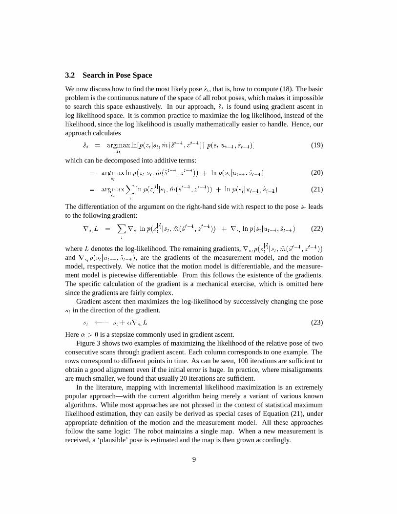
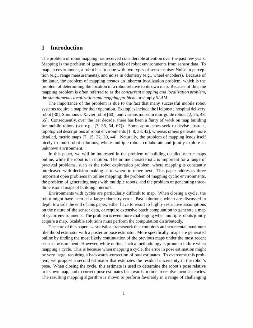
3.2 Search in Pose Space

We now discuss how to find the most likely posest, that is, how to compute (18). The basicproblem is the continuous nature of the space of all robot poses, which makes it impossibleto search this space exhaustively. In our approach,st is found using gradient ascent inlog likelihood space. It is common practice to maximize the log likelihood, instead of thelikelihood, since the log likelihood is usually mathematically easier to handle. Hence, ourapproach calculates

st = argmaxst

ln[p(ztjst; m(st�1; zt�1)) p(stjut�1; st�1)] (19)

which can be decomposed into additive terms:

= argmaxst

ln p(ztjst; m(st�1; zt�1)) + ln p(stjut�1; st�1) (20)

= argmaxst

Xi

ln p(z[i]t jst; m(st�1; zt�1)) + ln p(stjut�1; st�1) (21)

The differentiation of the argument on the right-hand side with respect to the posest leadsto the following gradient:

rstL =Xi

rst ln p(z[i]t jst; m(st�1; zt�1)) + rst ln p(stjut�1; st�1) (22)

whereL denotes the log-likelihood. The remaining gradients,rstp(z[i]t jst; m(st�1; zt�1))

andrstp(stjut�1; st�1), are the gradients of the measurement model, and the motionmodel, respectively. We notice that the motion model is differentiable, and the measure-ment model is piecewise differentiable. From this follows the existence of the gradients.The specific calculation of the gradient is a mechanical exercise, which is omitted heresince the gradients are fairly complex.

Gradient ascent then maximizes the log-likelihood by successively changing the posest in the direction of the gradient.

st � st + �rstL (23)

Here� > 0 is a stepsize commonly used in gradient ascent.Figure 3 shows two examples of maximizing the likelihood of the relative pose of two

consecutive scans through gradient ascent. Each column corresponds to one example. Therows correspond to different points in time. As can be seen, 100 iterations are sufficient toobtain a good alignment even if the initial error is huge. In practice, where misalignmentsare much smaller, we found that usually 20 iterations are sufficient.

In the literature, mapping with incremental likelihood maximization is an extremelypopular approach—with the current algorithm being merely a variant of various knownalgorithms. While most approaches are not phrased in the context of statistical maximumlikelihood estimation, they can easily be derived as special cases of Equation (21), underappropriate definition of the motion and the measurement model. All these approachesfollow the same logic: The robot maintains a single map. When a new measurement isreceived, a ‘plausible’ pose is estimated and the map is then grown accordingly.

9

(a) Initial match (e) Initial match

(b) After 10 iterations (f) After 10 iterations

(c) After 50 iterations (g) After 50 iterations

(d) After 100 iterations (h) After 100 iterations

Figure 3: To examples of gradient ascent for aligning scans (arranged vertically). In both cases, the initialtranslational error is 10 cm along each axis, and the rotational error is 30 degrees. The gradient ascent algorithmsafely recovers the maximum likelihood alignment.

10

-mismatch

-robot

6

path

Figure 4: A typical map obtained using the most simple incremental maximum likelihood approach. While themap is locally consistent, the approach fails to close the cycle and leads to inconsistent maps. This elucidates thelimitations of stepwise likelihood maximization, andillustrates the difficulty of mapping cyclic environments.

4 Incremental Mapping Using Posteriors

Unfortunately, the incremental maximum likelihood approach suffers a major drawback:It is inapplicable to cyclic environments. This limitation was recognized by Gutmann andKonolige [23] and others [39, 66]. Figure 4 depicts the map obtained in a cyclic environ-ment. Here the map appears to be locally consistent. However, local likelihood maximiza-tion still suffers a residual error thataccumulates over time. At the time the robot closes thecycle, the error has grown to a reputable amount, making it impossible to generate a mapthat is locally consistent. The magnitude of the error can grow without bounds, depend-ing on the robot’s odometry and the size of the cycle. Hence, the incremental maximumlikelihood approach is brittle.

Technically, the inability to close cycles is caused by two factors. Firstly, the method isunable to revise poses backwards in time. This is necessary when a cycle is closed to regainlocal consistency. Secondly, the robot maintains only a single hypothesis as to where it is.The unawareness of its own uncertainty may prevent the robot from finding a good matchwhen closing a cycle. Gradient methods only work well if the initial estimate is within thebasin of attraction of the maximum likelihood estimate. Since the error can grow withoutbounds, the initial estimate might be arbitrarily far away from the best match when closinga cycle. The resulting map is then usually unusable.

11

4.1 Pose Posterior Estimation

To remedy this problem, we will now discuss a hybrid estimation approach. This approachextends the incremental maximum likelihood algorithm by a second estimator, which es-timates the full posterior over poses (but not maps!). The posterior over poses is givenby

p(stjdt; m) = p(ztjst; m)

Zp(stjut�1; st�1) p(st�1jd

t�1; m) dst�1 (24)

This equation is obtained by substituting the poses for x in (2), and conditioningeverythingon the mapm (except for the robot motion). It is essentially equivalent to the Markov local-ization algorithm, a popular algorithm for mobile robot localization with known maps [3,27, 49, 62]. However, Markov localization assumes the availability of a complete map ofthe environment, which is not assumed here.

The key reason for memorizing the full posteriorp(stjdt; m), instead of the maximum

likelihood estimatest only, it our desire to accommodate the increasing residual uncertaintywhen moving into unmapped terrain. As the robot traverses a cycle, the posterior growsincreasingly large, and the posterior characterizes this uncertainty.

Formally, the posterior is obtained by substituting the maximum likelihoodmapm(st�1; zt�1)

into Equation (24), which gives us

p(stjdt; m(st�1; zt�1)) = p(ztjst; m(st�1; zt�1)) (25)Z

p(stjut�1; st�1) p(st�1jdt�1; m(st�1; zt�1)) dst�1

Notice the difference between this estimator and the one in (17). Equation (17) computesthe posterior over poses and maps; here we assume knowledge of the map and computethe posterior over poses only. This frees us of the necessity to calculate the most likelypose and instead enables us to maintain a full posterior over all poses. On the other hand,calculating (25) requires integration, whereas (17) does not. Luckily, the integration is well-understood in the rich literature on Markov localization, and below we will adopt one of therepresentations developed there.

Knowledge of the posterior gives us a better way to calculate the maximum likeli-hood pose�st. In particular,�st is obtained by maximizing the posterior (25), instead ofthe marginal posterior specified in Equation (17):

�st = argmaxst

p(stjdt; m(st�1; zt�1)) (26)

The resulting pose is generally the same when mapping unexplored terrain. However, itmay differ when closing a cycle, at which point the robot might have to compensate a largepose error.

This consideration points out the key advantage of maintaining the full posterior, insteadof the most likely pose only. Our approach fundamentally addresses one of the two problemsdiscussed above, namely that of errors growing without bounds when closing a cycle. The

12

Figure 5: Sample-based approximation for the posterior over poses. Here each density is represented by aset of samples, weighted by numerical importance factors. The Monte Carlo localization algorithm is used togenerate the sample sets.

posterior estimator can accommodate such errors. In particular, when closing a cycle theposterior provides a spectrum of hypotheses as to where the robot might be. The samplerepresentation, described in turn, provides a set of potential seeds for the gradient ascentsearch, which makes it possible to find best matches when closing arbitrary large cycles.

4.2 Approximation Using Monte Carlo Localization

Our algorithm implements the posterior calculation using particle filters [13, 14, 38, 51].Particle filters apply Rubin’s idea of importance sampling [55] to Bayes filters. The result-ing algorithm is known in computer vision ascondensation algorithm[26], and in mobilerobotics asMonte Carlo localization[10, 17, 34]. A similar algorithm has been proposedin the context of Bayes networks as [29]survival of the fittest.

Particle filters represent the posteriors by a set of particles (samples). Each particle isa pose that represents a ‘guess’ as to where the robot might be. Particle filters weigh eachparticle by a non-negative numerical factor, commonly referred to asimportance factor.Figure 5 shows an example of the particle representation in the context of mobile robotlocalization. Shown there is a sequence of posterior beliefs for a robot that follows a U-shaped trajectory. Each of the sample sets is an approximation of densities (of the typeshown in Figure 1).

The general algorithm is depicted in Table 1. When transitioning from timet�1 to timet, new particles are generated by sampling poses from the current posterior and guessing asuccessor pose using the motion model. The weight of the particle is then obtained using themeasurement model. Particle filters have been shown to approximate the Bayes filter updateequation given in (2). As argued in the statistical literature, the particle representation canapproximate almost arbitrary posteriors at a convergence rate of1p

N[64]. It is convenient

13

Algorithm particle filter(Xt�1; ut�1; zt):

for i = 1 to n to

samplexhiit�1 fromXt�1 according to the importance factorswhjit�1 in Xt�1

samplexhiit � p(xtjut�1; xhiit�1)

setwhiit = p(otjx

hiit )

addhxhiit ; whiit i toXt

endfor

normalize all weightswhiit in Xt so that they sum up to 1.

returnXt

Table 1: The particle filter algorithm. This algorithm is an approximate version of Bayes filters that usesparticles to represent the posterior belief. The input is a weighted particle setXt�1 representingp(xt�1jd

t�1),along with a controlUt�1 and a measurementzt. The output is a new weighted set ofn particles representingp(xtjd

t).

for robotics, since it is easy to implement, and both more efficient and more general thanmost alternatives [17].

In the context of mapping, the application of particle filters and MCL for posterior esti-mation is straightforward. At each point in time, the robot has access to the map built frompast data. Another key advantage of the particle representation is that directly facilitates theoptimization of (26) using gradient ascent. Our approach performs gradient ascent usingeach sample as a starting point, then computes the goodness of the result using the obviouslikelihood function. If the samples are spaced reasonably densely (which is easily done withonly a few dozen samples), one can guarantee that the global maximum of the likelihoodfunction can be found. This differs from the simple-minded approach above, where only asingle starting pose is used for hill-climbing search, and which hence might fail to producethe global maximum (and hence a usable map).

4.3 Backwards Correction

As argued above, when closing cycles it is imperative that maps are adjusted backwards intime. The amount of backwards correction is given by the difference�st :

�st = �st � st (27)

wherest is as defined in (21) and�st as in (26), respectively. This expression is the differencebetween theincrementalbest guess (c.f., our base-line approach) and the best guess usingthe full posterior.

If �st = 0, which is typically the case whennotclosing a loop, no backwards correctionhas to take place. When�st 6= 0, however, a shift occurred due to reconnection with apreviously mapped area, and poses have to be revised backwards in time.

14

(a) (b)

Figure 6: Robots: (a) Two of the pioneer robots used for multi-robot mapping. (b) Urban robot for indoorand outdoor exploration. The urban robot’s odometry is extremely poor. All robots have been manufactured byRWI/ISR.

Our approach does this in three steps:

1. First, the size of the loop is determined by determining the scan in the map which led tothe adjustment (this is a trivial side-result in the posterior computation).

2. Second, the error�st is distributedproportionallyamong all poses in the loop. This com-putation doesnotyield a maximum likelihood match; however, it places the intermediateposes in a good starting position for subsequent gradient ascent search.

3. Finally, gradient ascent search is applied iteratively for all poses inside the loop, untilthe map is maximally consistent (maximizes likelihood) under this new constraint arisingfrom the cycle.

These three steps implement an efficient approximation to the maximum likelihood estima-tor for the entire loop. Strictly speaking, this approach is not an online algorithm any longer,since the time required for backwards correction is not constant. A remedy might be foundby amortizing the costs of the loop over the time used to acquire the next one. However,we found that in practice the entire correction can well be performed between subsequentrange measurements, for all environments discussed in the experimental result section ofthis paper.

5 Results for Single-Robot Mapping

We validated the basic algorithm in various different environments. The mapping algorithmwas at the core of several demonstrations to Government officials in DARPA’s TacticalMobile Robot (TMR) program. The role of CMU’s Mercator project was to demonstratethe feasibility of rapidly acquiringaccurate maps of building interiors with mobile robots.Our experiments are aimed at illustrating the robustness andaccuracy of our approach inenvironments that traditionally are difficult to map.

The majority of the results discussed below were obtained with the robots shown inFigure 6. Figure 6a shows two RWI Pioneer AT robots, which were modified by replacing

15

two of the wheels with passive casters (the original skid-steering mechanism was unable toturn on carpet). Figure 6b shows a tracked robot known asurban robot, also developed byRWI/ISR. This highly versatile robot has been developed for the DARPA TMR program,for indoor and outdoor missions in rugged terrain.

Our first experiment is concerned with closing the cycle in cyclic environments. Fig-ure 7 shows different stages of mapping. using the very same data as in Figure 4. Here,however, the posterior estimator is used to detect and correct inconsistencies when closingthe cycle. The particles are also shown in Figure 7, along with the most likely robot pose.As is easily seen, the resulting map is now consistent. Moments before the cycle is closed,the accumulated error is approximately 50 centimeters, as shown in Figure 7b. When clos-ing the cycle, the most likely pose is adjusted in accordance to the previously mapped area,thereby practically eliminating this error. The backwards correction mechanisms then dis-tributes the adjustment along the cycle, and the new, improved map is generated in less thana second of processing time. Figure 7c shows the final map.

To test the robustness of the mapping algorithm in the extreme, we manually deprivedthe data of its odometry information. Hence, only the laser range data can be used toestimate the robot’s pose. Odometry-free mapping tests the robustness of the algorithm.If an algorithm can generate a consistent map without odometry data, it can accommodatefailure of a robot’s wheel encoders or INU (inertial navigation unit). Clearly, odometry-freemapping can only succeed if the environment possesses sufficiently distinguishing features.For example, without odometry it would be impossible to map a wide open area where allobstacles are beyond the reach of the sensors, or very long, featureless hallways.

Figure 8 shows the result of mapping the cyclic environmentwithout odometry. Fig-ure 8a depicts the raw data which, without odometry, is difficult to interpret. The map inFigure 8b has been generated using the statistical technique described in this paper. In par-ticular, the same set of parameters were used to construct this map, as if the odometry datawas available. This sheds light on the robustness of our approach.

Mapping with poor odometry has practical significance, as not all mobile robots havegood odometry. A particularly inaccurate robot is the urban robot shown in Figure 6b. Fig-ure 9a depicts a raw data set gathered while the robot was autonomously exploring andmapping a military facility in Fort Sam Houston in Texas. While the odometry is quite ac-curate when the robot moves straight, its tracks introduce up to 100% rotational error whenthe robot rotates. Thus, odometry alone is unusable even over very short time intervals. Themap of this non-cyclic environment is shown in Figure 9b, along with the robot’s explo-ration path. This map is not perfect, as attested by the fact that the walls are not perfectlyaligned. However, is is sufficiently accurate for navigation.

A final result was obtained in a public place, the Tech Museum in San Jose, Califor-nia. A key feature of this environment is the availability of anaccurate blueprint, whichenables us to evaluate the accuracy of the map acquired by the robot. The specific map wasacquired with a RWI B21 robot. Figure 10a shows an occupancy grid map [15, 44] of alarge center area in the museum, extracted from the aligned scans. A comparison with thearchitectural blueprint of the museum in Figure 10b illustrates that the learned map is quite

16

(a)

���

robotand samples

(b)

���

robot andsamples

(c)

� robot and samples

Figure 7: Incremental algorithm for concurrent mapping and localization. The dots, centered around the robot,indicate the posterior belief which grows over time (a and b). When the cycle is closed as in (c), the posteriorbecomes small again.

17

Figure 8: Mapping without odometry. Left: Raw data, right: map, generated online.

accurate. Several differences between these maps stem from the fact that the blueprint doesnot accurately reflect the nature and location of the exhibits in the museum. In this regard,the map learned by the robot is more accurate than the museum’s blueprint.

6 Multi-Robot Mapping

The extension of our algorithm to multi-robot mapping is quite straightforward. In themulti-robot mapping problem, multiple robots gather data concurrently in an attempt tobuild a single, unified map of the environment. The use of multiple robots is advantageousif the speed at which a map is being constructed is important: In the best case, the speed-up by usingN robots instead of one is super-unitary: In theory, environments exist whereN robots consume approximately1

2Nthe time it would take a single robot to map the

environment. The factor 2 arises from the fact that in some environments, a single robotmight waste time traversing known territory to get back to places not yet visited. In practice,however, the speedup is usually sub-linear [61].

Our current implementation makes two important restrictive assumptions:

� First, the robots must begin their operation in nearby locations, so that their range scansshow substantial overlap.

� Second, the software must be told the approximate relative initial pose of the robots. Theaccuracy of the initial estimate is bound by the basin of attraction of the gradient ascentalgorithm. A safe error is usually up to 50 cm and 20 degrees in orientation.

Under these conditions, the extension to multi-robot mapping is straightforward. In particu-lar, each robot maintains a local, robot-specific estimate of its pose, while sharing the same

18

Figure 9: Autonomous exploration and mapping using the urban robot: Raw data and final map, generated inteal-time during exploration.

map. The estimation of the most likely pose using the incremental maximum likelihoodestimator is based on a single, global map that fuses data collected by all robots.

Put mathematically, if we usek to index each particular robot, the posterior over thek-th robot pose is given by

p(st;kjdtk; m) = p(zt;kjst;k; m)

Zp(st;kjut�1;k; st�1;k) p(st�1;kjd

t�1k ; m) dst�1;k

(28)

This equation generalizes Equation (24) to the multi-robot case with a single global mapm.The most likely pose of thek-th robot is then determined by generalizing Equation (26):

�st;k = argmaxst;k

p(st;kjdtk; m(st�1

k ; zt�1k )) (29)

where the functionm incrementally grows the global mapm. This extensions exploit thefact that none of the underlying statistics crucially depends on the number of robots. Italso exploits an interesting conditional independence that enables us to factorize the poste-rior distribution of the joint pose space. In particular, the commitment to maximum likeli-hood maps eliminates possible dependencies between the pose estimates of different robots,which otherwise exist for the full Bayesian solution. Thus, in the general context, the poste-rior over robot poses would have to be estimated jointly, but here we can estimate it locallyon each robot (see [18] for a more detailed discussion). We notice that the pose estimationcan be carried out locally, on each robot. This leads to a computationally elegant decompo-sition of the problem, in whicheach robot basically performs the same basic algorithm asin single-robot mapping, but map updates are broadcast to all robots.

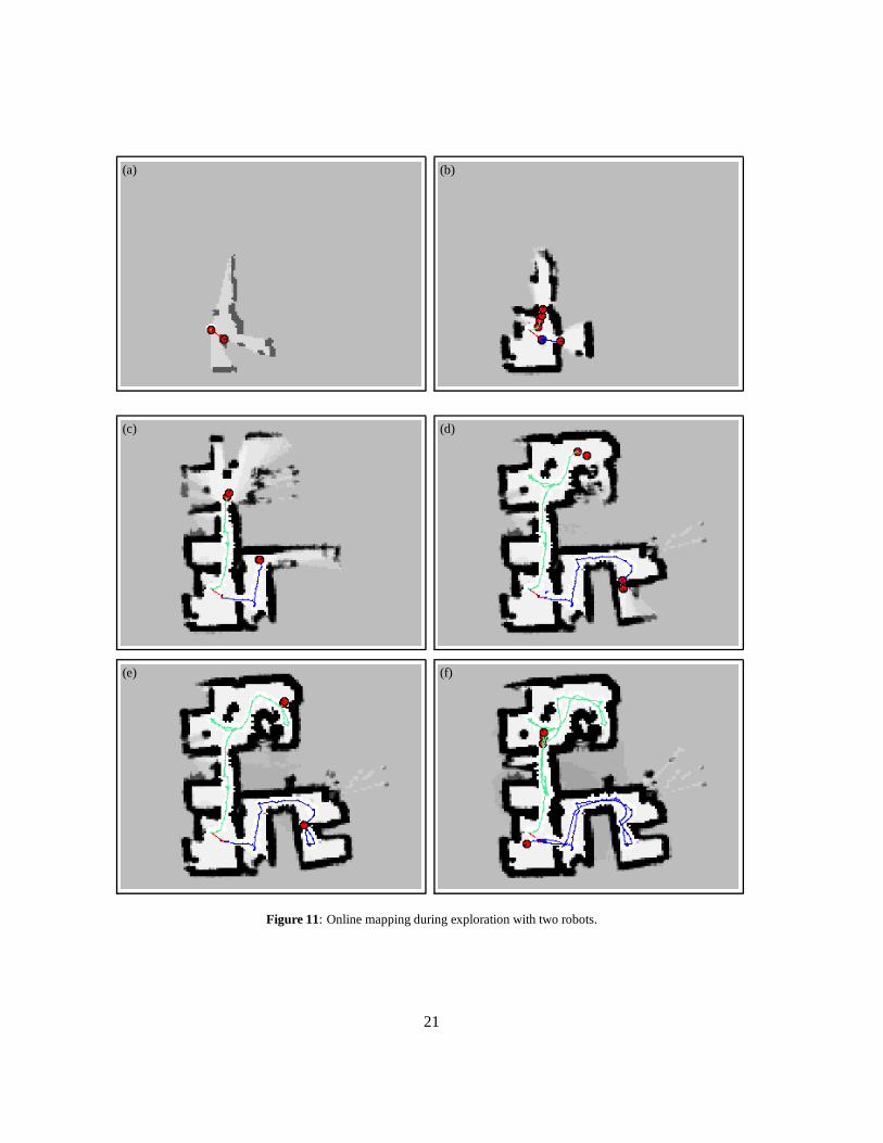
Figure 11 shows a map built by two autonomously exploring robots. This experimentwas carried out in a TMR demonstration that took place in a training facility for firefighters

19

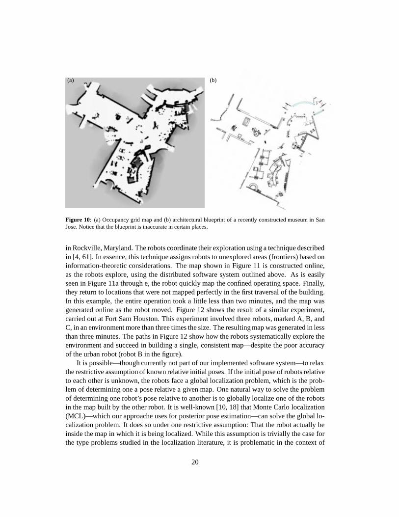
(a) (b)

Figure 10: (a) Occupancy grid map and (b) architectural blueprint of a recently constructed museum in SanJose. Notice that the blueprint is inaccurate in certain places.

in Rockville, Maryland. The robots coordinate their exploration using a technique describedin [4, 61]. In essence, this technique assigns robots to unexplored areas (frontiers) based oninformation-theoretic considerations. The map shown in Figure 11 is constructed online,as the robots explore, using the distributed software system outlined above. As is easilyseen in Figure 11a through e, the robot quickly map the confined operating space. Finally,they return to locations that were not mapped perfectly in the first traversal of the building.In this example, the entire operation took a little less than two minutes, and the map wasgenerated online as the robot moved. Figure 12 shows the result of a similar experiment,carried out at Fort Sam Houston. This experiment involved three robots, marked A, B, andC, in an environment more than three times the size. The resulting map was generated in lessthan three minutes. The paths in Figure 12 show how the robots systematically explore theenvironment and succeed in building a single, consistent map—despite the poor accuracyof the urban robot (robot B in the figure).

It is possible—though currently not part of our implemented software system—to relaxthe restrictive assumption of known relative initial poses. If the initial pose of robots relativeto each other is unknown, the robots face a global localization problem, which is the prob-lem of determining one a pose relative a given map. One natural way to solve the problemof determining one robot’s pose relative to another is to globally localize one of the robotsin the map built by the other robot. It is well-known [10, 18] that Monte Carlo localization(MCL)—which our approache uses for posterior pose estimation—can solve the global lo-calization problem. It does so under one restrictive assumption: That the robot actually beinside the map in which it is being localized. While this assumption is trivially the case forthe type problems studied in the localization literature, it is problematic in the context of

20

(a) (b)

(c) (d)

(e) (f)

Figure 11: Online mapping during exploration with two robots.

21

AB

C

Figure 12: Map built by three autonomously exploring robots. The initial robot poses are on the left as markedby the letters A, B, and C. The robots A and C are pioneers, and the robot B is an urban robot.

multi-robot mapping. In particular, two robots might start out in different, non-overlappingparts of a building, and hence none of the robots operates inside the map built by any of theother robots. Thus, to estimate the poses of robot relative to each other, the robots must beable to estimate the degree of overlap between the areas traversed thus far. Clearly, MCLprovides no answer to this hard and important problem.

However, MCL can be applied if it is known that one robot starts in the map built byanother. Such a situation is shown in Figure 13. Here one robot is declared theteam leader,which builds an initial, partial map. The second robot is then placed somewhereinsidethismap, but its pose inside this map is unknown. The particle filter of the second robot is theninitialized by a set of particles drawn uniformly across the map of the first robot. The exactsame posterior estimator depicted in Table 1 is then applied to globally localize the secondrobot in the map built by the team leader. Figure 13a shows the posterior after integratingone measurement. In this specific example, the samples have been generated in proximityto the first robot’s path, assuming the second robot starts out near a location where theteam leader has been before. A few moments later, the relative pose has been determined(Figure 13b) and the robot begins contributing data to the same, global map (Figure 13c).

7 3D Structural and Texture Mapping

A second extension of the basic mapping algorithm is the idea of three-dimensional maps.Such maps can be informative to people interested in a virtual view of a building interior.

22

(a)���

robot

� team leader

(b)���

robot

� team leader

(c)

���robot

� team leader

Figure 13: A second robot localizes itself in the map of the first, then contributes to building a single unifiedmap. In (a), the initial uncertainty of the relative pose is expressed by a uniform sample in the existing map.The robot on the left found its pose in (b), and then maintains a sense of location in (c).

For example, it enables to pay a virtual visit using VR interfaces without actually physicallyentering the building. This might be useful for architects, real estate agents, and also forpeople preparing to operate in hazardous environments such as nuclear waste sites.

Figure 14a shows a robot equipped with two laser range finders. One of the laser rangefinders is pointed forward, to generate a 2D map using the techniques described above. Asa result, it provides the robot with accurate pose estimates. The second laser range finderis mounted vertically, so that the light plane is perpendicular to both the first range scanner,and the motion direction of the robot. As a result, this range scanner measures cross-sectionsof the building as the robot moves. If the robot traverses the environment only once—whichis typically the case in exploration—the measurements of the upward-pointed laser do notoverlap; hence, there is little hope of using it for localization. However, the data providesinformation about the 3D structure of the building.

The robot shown in Figure 14a is also equipped with a panoramic camera. The panoramiccamera utilizes a small mirror, which provides an image that contains the area covered bythe upward-pointed laser range scanner. The mirror is mounted only a few centimeters awayfrom the optical axis of the laser range scanner. Careful calibration of both devices enable usto match range and color measurements along the measurement plane of the vertical rangefinder, basically ignoring the small disparity between the optical axes of the laser and thecamera. Figure 14 shows a panoramic image. The curved line highlights a vertical cross-section of the building, which corresponds to the perceptual field of the upward-pointedlaser range finder.

Our approach represents 3D maps as collections of polygons with texture superimposed.Our 3D mapping algorithm proceeds in five steps, all of which can be carried out online.

1. Pose estimation:Pose estimation is carried out in 2D, using the techniques describedabove. The vertical range data is then projected into global coordinates using the maxi-mum likelihood pose�s.

2. Raw data smoothing:Local noise in the range measurements is reduced by local smooth-

23

(a) (b)

Figure 14: (a) Pioneer robot equipped with 2 laser range finders and panoramic camera used for 3D mapping.(b) Panoramic image acquired by the robot. Marked here is the region in the image that corresponds to thevertical slice measured by the laser range finder.

ing. Neighboring sensor scans are smoothed by replacing them with a locally weightedaverage, using a smoothing kernel of size 3 by 3. This step yields significantly smoothersurfaces in the final map.

3. Structural Mapping: The map is then built by searching nearby range scans for nearbymeasurements. More specifically, for each time� and indexi, for which the coordinatesof the four measurements

z[i]� ; z[i+1]� ; z

[i]�+; z

[i+1]�+ (30)

are less than� apart in 3D coordinates, these points are assumed to correspond to thesame objects. Hence, a polygon is generated with the endpoints corresponding to thosefour measurements and added to the map. Notice that polygon’s are only constructed formeasurements recorded right after another, and for neighboring sensor beams. The testof adjacency in 3D space is essential, since large discontinuities often correspond to openspace (e.g., an open door).

4. Texture Mapping: If a polygon is generated, the image sequence recorded between thetimes� and� +1 are used as texture for the polygon. In particular, our algorithm extractsfrom the camera image a stripe that corresponds to the perceptual range of the laser.Stripes are then concatenated, which generates a texture image for the entire range scan,and the region corresponding to the area between thei-th and the(i + 1)-th range scanare extracted using a straightforward geometrical argument. This texture is then mappedonto the polygon.

5. Map simplification: To simplify the maps, the polygons are finally fused by a softwarepackage developed by computer graphics researchers [20, 21]. This approach, which oursoftware uses without modification, fuses polygon’s based on a quadratic error measureson their appearance in the rendered image. We found that the number of polygons can be

24

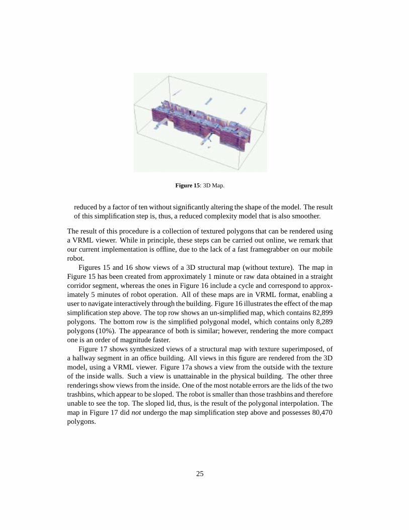
Figure 15: 3D Map.

reduced by a factor of ten without significantly altering the shape of the model. The resultof this simplification step is, thus, a reduced complexity model that is also smoother.

The result of this procedure is a collection of textured polygons that can be rendered usinga VRML viewer. While in principle, these steps can be carried out online, we remark thatour current implementation is offline, due to the lack of a fast framegrabber on our mobilerobot.

Figures 15 and 16 show views of a 3D structural map (without texture). The map inFigure 15 has been created from approximately 1 minute or raw data obtained in a straightcorridor segment, whereas the ones in Figure 16 include a cycle and correspond to approx-imately 5 minutes of robot operation. All of these maps are in VRML format, enabling auser to navigate interactively through the building. Figure 16 illustrates the effect of the mapsimplification step above. The top row shows an un-simplified map, which contains 82,899polygons. The bottom row is the simplified polygonal model, which contains only 8,289polygons (10%). The appearance of both is similar; however, rendering the more compactone is an order of magnitude faster.

Figure 17 shows synthesized views of a structural map with texture superimposed, ofa hallway segment in an office building. All views in this figure are rendered from the 3Dmodel, using a VRML viewer. Figure 17a shows a view from the outside with the textureof the inside walls. Such a view is unattainable in the physical building. The other threerenderings show views from the inside. One of the most notable errors are the lids of the twotrashbins, which appear to be sloped. The robot is smaller than those trashbins and thereforeunable to see the top. The sloped lid, thus, is the result of the polygonal interpolation. Themap in Figure 17 didnot undergo the map simplification step above and possesses 80,470polygons.

25