An object-oriented framework for simulating supply systems · An object-oriented framework for simulating supply systems MD Rossetti*, M Miman and V Varghese ... to a simulation-based

UNCORRECTED PROOF

An object-oriented framework for simulatingsupply systemsMD Rossetti*, M Miman and V Varghese

University of Arkansas, Fayetteville, AR, USA

A framework is a set of reusable classes that work together to facilitate the construction of software within a particulardomain. In this paper, we present an object-oriented framework for developing simulation models involving supplychain networks. The key object-oriented artefacts for modelling inventory-based supply chain networks are presentedincluding the classes, their attributes, relationships, and behaviours. The framework’s implementation within Javais also presented through a number of examples. The examples illustrate the capabilities of the framework to buildlarge-scale multi-echelon, multi-item inventory networks with time-based transport between locations.Journal of Simulation (2008) 0, 000–000. doi:10.1057/jos.2008.2

Keywords: inventory; logistics; simulation; object-oriented

1. Introduction

We conceptualize a supply chain as a network of facilities

and distribution options that allow products to flow from

suppliers to customers. We present a general-purpose object-

oriented framework for developing simulation models of

supply chains. While other more general network structures

can be easily modelled with our framework, we concentrate

on illustrating the framework on supply networks that have

an arborescent tree of inventory holding points (IHPs) as

illustrated in Figure 1. In an arborescent network, each IHP

can have one and only one supplier; however, our frame-

work is not limited in this respect. We will discuss how to

handle the case of many to many relationships between IHPs

later in this document.

Each IHP is a location within the network that can stock

inventory item types (ie stock keeping units or SKUs). At the

top of the network is a supplier that can supply any item type

with a possible lead-time. The top-level supplier essentially

acts as an external supplier for the top level of the tree. An

IHP at any level can supply one or more customers (eg other

IHPs). The bottom most level of the hierarchy receives

requests for demand for inventory from external customers.

This type of structure forms the general class of inventory

systems called multi-echelon inventory systems. From a

supply chain perspective, looking up from the bottom of the

tree back to the external supplier, we have the customer’s

supply chain. In such situations, it is useful to understand the

effect of inventory stocking location, demand, transport

delay, control policy, etc on the performance of the system.

While analytical models do exist for specific multi-echelon

inventory system configurations, the wide variety of condi-

tions under which such systems operate is often better suited

to a simulation-based approach to evaluating system

performance. In this paper, we describe an object-oriented

framework that allows the easy development and simulation

of systems like that shown in Figure 1 and can serve as a

foundation for developing much more complicated models.

For example, the spare parts network that we illustrate in a

later section was easily developed by simply sub-classing

from or using the available components within the basic

framework. Besides the implementation of relatively

standard multi-echelon situations, the framework can also

model more dynamic supply situations. For example, in an

emergency planning context, we can have suppliers lose their

ability to support certain items or locations and to

dynamically gain the ability to support other items and

locations based on events or other control logic.

In our framework there are no physical limitations (except

for memory) that limit the size of the model (eg number of

echelons, retailers, inventory items, allocation of inventory

to each IHP, etc). The framework is based on the Java

programming language and thus assumes that the modeller

can program in a general-purpose object-oriented language

such as Java. As we will see in our illustrative examples, even

non-programmers could build relatively complex models by

following the outline presented in our examples. In addition,

because the software is open-source it could easily be

embedded in a more sophisticated graphical user interface

package that takes advantage of the full features of the Java

language (eg dialog boxes, databases, etc). From that

perspective, we expect a variety of potential users from

researchers in academia to practitioners in industry and the

military. Note that class diagrams provided in this paper as

Journal: JOS Disk used OP: KGU Ed: PRASADArticle : ppl_jos_4250039 Pages: 1–14 Despatch Date: 2/2/2008

Gml :Template: Ver 1.1.5

*Correspondence: MD Rossetti, Industrial Engineering Department, 4207Bell Engineering Center, University of Arkansas, Fayetteville, AR 72701,USA.E-mail: [email protected]

Journal of Simulation (2008) 0, 1–14 r 2008 Operational Research Society Ltd. All rights reserved. 1747-7778/08 $30.00

www.palgrave-journals.com/jos

UNCORRECTED PROOF

well as Figure 3 can help potential users to conceptualize the

abilities of the framework.

This paper represents an expansion of the work in

Rossetti et al (2006) and also presents new modelling

concepts/examples in an expository fashion. Our intention is

not to analyse or optimize a particular supply chain

situation. Rather, our purpose is to describe the modelling

foundation and capabilities of our supply chain simulation

framework through discussion and examples. This should

serve as a basis for researchers and practitioners who might

be interested in using the framework and it should provide a

better understanding of general methods to model logistic

systems.

The rest of this paper is structured as follows. In the next

section, we present a brief overview of the literature in this

area to give context for how our framework fits into this

modelling area. Then, we introduce the framework by

discussing the elements for modelling inventory stocked at a

single location. This will cover the modelling of classic

inventory situations such as reorder point and order up to

systems. Then, we describe how the framework can use the

basic inventory modelling components to build models with

multiple locations, stocking multiple item types with

transport between locations. Finally, we summarize and

discuss future research.

2. Literature review

Previous research in supply chain simulation modelling can

be roughly classified into two main areas: applications of

simulation modelling to supply chain analysis and develop-

ment of modelling approaches or tools to better facilitate

the simulation of supply chains. For example, the paper by

Schunk and Plott (2000) describes the application of

simulation to the optimization of supply chain management

activities through modelling. Moreover, Li and Zhao (2006)

apply an adaptive multi-agent modelling method to agile

supply chain simulation, and illustrate the concrete model-

ling process within the context of a task allocation problem.

In addition, interested readers can find an extensive study

that surveys different types of simulation for supply chain

management and discusses several methodological issues in

this area provided by Kleijnen (2005). Overall, these many

applications of simulation to supply chain analysis have led

researchers to conclude that simulation is one of (if not the

best way) to truly analyse dynamic supply chain perfor-

mance. For example, Dong (2001) considered simulation as

a better technology for designing supply chain systems due

to the system variation and interdependencies. In addition,

Ingalls (1998) concluded that simulation is the best method

to analyse supply chain systems where the key driver is

variance. Unfortunately, while simulation facilitates the

analysis of complex supply chains it has the disadvantage

of requiring large amounts of data and taking a long time to

develop.

Because of the challenges of applying simulation to supply

chain modelling, researchers (and commercial entities) have

taken an interest in developing better modelling tools. Early

attempts at developing tools in this area date back to the late

1960s and early 1970s. For example, Bowersox et al (1972)

describe a complete FORTRAN-based supply chain simu-

lator that also incorporated optimization procedures to

simulate and design physical distribution systems. More

recently, a common approach is to develop a tool to analyse

a company’s supply chain. For example, the paper by Ingalls

and Kasales (1999) combines both the analysis of a supply

chain (for Compaq computer) and the development of a tool

that can more easily allow such an analysis over time. These

tools often take the form of supply chain simulators. In this

line, there are many commercial off the shelf simulators such

as SCOPE, SIMLOX, and LogSAM, which have been

applied in military supply chains.

The Supply Chain Operations Reference (SCOR) model is

widely accepted as the cross-industry standard for supply

chain management. Several supply chain simulators were

developed in the past of which IBM Supply Chain Simulator

(SCS) is an important one based on ideas in SCOR. Bagchi

et al (1998) gives a brief outline on the components in SCS

and describes how it was used in the modelling of two

PPL_JOS_4250039

Level 3: External Supplier

Level 2 Warehouses

Level 1 Retailers

S

1

1 2

2 k

1 2 m2m1 1 2 mk

Figure 1 An arborescent supply chain structure.

Q1

2 Journal of Simulation Vol. ] ], No. ] ]

UNCORRECTED PROOF

diverse industries (Food Industry and Computer Industry).

The SCS allows detailed costing and financial analysis to be

made based on the simulation of a supply chain. Smart-

SCOR is a new addition to IBM’s arrays of tools for supply

chain management and it conforms to the SCOR standards.

It facilitates supply chain transformations. A supply chain

transformation initiative consists in changing the ways in

which an enterprise forms and operates its supply chain,

concerning the decisions from supply chain network

rationalization to business process re-engineering. Smart-

SCOR sees transformation in two different levels, from

supply chain strategy design/redesign to supply chain

process improvement (Dong et al, 2006). In addition,

Pundoor and Herrmann (2006) developed a supply chain

simulation framework based on the SCOR model. This

framework has been used for building simulation models

that integrate discrete event simulation and spreadsheets.

The simulation models are hierarchical and use sub-models

that capture activities specific to supply chains. The SCOR

framework provides a basis for defining the level of detail in

such a way that it includes as many features as possible,

while not being industry specific. Their approach enables the

reuse of sub-models, which reduces the model development

time. They describe the implementation of the simulation

models and detail how the sub-models interact with each

other. A similar framework based on SCOR and through

identification of standard applications, the right level of

abstraction, and associated requirements for data has been

developed by Jain (2007). Finally, Chatfiled et al (2006)

presents the software (SISCO) for the storage, modelling,

and generation of supply chains where the user specifies the

structure and policies of a supply chain with a GUI-based

application and then saves the supply chain description in

the open, XML-based Supply Chain Modelling Language

(SCML) format. SISCO automatically generates the simula-

tion model when needed by mapping the contents of the

SCML file to a library of supply-chain-oriented simulation

classes. Their methodology is an object-oriented, agent-style

system architecture.

A reader interested in understanding our other research in

this area should refer to Rossetti et al (2006), Rossetti and

Chan (2003), Rossetti and Thomas (2006). In particular,

Rossetti et al (2006) overviews other software architectures

(eg Swaminathan, 1998) and approaches for simulating

supply chains. In the following section, we discuss the basic

building block for our framework based on the inventory

layer of the supply chain.

3. Inventory modelling

In our modelling, we have identified a key abstraction for the

modelling of supply chains, which we term the inventory

layer. The other layers in our overall framework include a

facility layer and a transport layer. In this paper, we

primarily discuss the inventory layer. We do this by

describing the object-oriented constructs within the layer

and by illustrating their use.

Our object-oriented framework is built upon a Java

Simulation Library (JSL), which is described in Rossetti

(2007). The JSL is an open source simulation library for

Java. The JSL has packages that support random number

generation, statistical collection, basic reporting, and

discrete-event simulation modelling. The development of a

simulation model is based on sub-classing the ModelElement

class that provides the primary recurring actions within a

simulation and event scheduling/handling. The user develops

and instantiates instance of subclasses of ModelElement.

The model elements are added to an instance of the Model

class or to other ModelElements. This facilitates the

modelling of a hierarchy of systems. Then, the user

instantiates an instance of the Experiment class so that the

simulation model can be executed. The JSL is divided into

Java packages (calendar, examples, modelling, spatial,

observers, and utilities) where each package is further

organized through sub-packages. The modelling package is

further divided into packages (processes, resources, queues,

transporters, etc) that facilitate more detailed modelling. In

this section, we will discuss a package developed to represent

the inventory layer within our framework.

3.1. Overview of key classes

The framework is predicated on the general notion of

modelling things that can fill demand and things that can

send demand. The DemandFillerIfc and the Demand-

SenderIfc interfaces represent these two concepts. In

addition, we have the concept of transporting demand

between senders and fillers represented by the DemandCar-

rierIfc interface. These three concepts as well as a rigorous

state transition pattern for instances of Demand allow the

very flexible modelling of general-purpose supply networks.

To make these general concepts concrete, the user must

implement the appropriate interfaces or abstract base

classes. The inventory package currently has 35 interfaces,

seven abstract base classes, and 56 classes that facilitate

inventory system modelling. Obviously, we cannot discuss

all of these classes in this paper. For basic modelling with the

inventory package, there are six key (concrete) classes that

must be well understood: ItemType, Demand, Demand-

Generator, Inventory, BackLogPolicyAbstract, and Inven-

toryPolicyAbstract. For simplicity in our discussion, we will

refer to instances of these classes by the lower case nouns

related to the class names whenever the context is clear. For

example, item type and demand refer to instances of

ItemType and Demand, respectively.

The class ItemType represents or describes the items or

products in the inventory system. The Demand class

represents a request for inventory and provides the status

of the request. A demand knows (has attributes for) the item

PPL_JOS_4250039

Q2

MD Rossetti et al—Object-oriented framework for simulating supply systems 3

UNCORRECTED PROOF

type associated with the request, the sender of the request,

the filler of the inventory items, the carrier of the items, the

amount of the request, and other customer requirements

associated with the request, such as whether backlogging or

partial filling is permitted. The DemandGenerator class

creates demands and acts as a customer that sends the

demand by providing details of the customer requirements.

The Inventory class represents units of a particular item type

that can be requested and keeps track of the amount of

inventory on-hand, backlogged, on order, etc. An instance

of the Inventory class represents the state of the inventory

at any given time. In addition, it provides methods for

requesting units of an item type and for filling demands for a

given item type. Every Inventory class is associated with an

inventory policy. The class, InventoryPolicyAbstract, is an

abstract base class that allows for the encapsulation of rules

to control the associated inventory; it is a rule, policy, or

strategy that governs the re-ordering behaviour for inven-

tory. An inventory policy determines when to order and how

much to order. Currently, a variety of different inventory

policies, such as continuous and periodic review policies,

have been implemented. In addition, a backlog policy can be

associated with the Inventory class. An abstract base class,

BackLogPolicyAbstract, represents the different rules or

behaviours that can be used to backlog demands for

inventory and to fill backlogs associated with inventory.

Figure 2 illustrates the behaviours and attributes of these six

classes as well as their relationships. For example, within

Figure 2, the class Inventory has a reference to a back log

policy as well as an inventory policy. Within the diagram,

instances of a DemandGenerator will know its demand filler

via an instance of Inventory.

The interactions between these classes are facilitated by

four key interfaces: DemandFillerIfc, DemandSenderIfc,

DemandCarrierIfc, and DemandStateChangeListenerIfc.

Again, where the context is clear, we will refer to instances

that implement these interfaces by the appropriate nouns

based on the name of the interface. For example, something

that implements the DemandFillerIfc interface will be called

a demand filler. The interface, DemandFillerIfc, represents

PPL_JOS_4250039

Figure 2 Relationships between key classes in inventory package.


UNCORRECTED PROOF

something that can receive demand to be filled. The class

Inventory implements this interface and thus promises to act

like a demand filler. A class, like DemandGenerator, that

implements the interface DemandSenderIfc specifies how it

will send demand while the interface, DemandCarrierIfc,

knows how to ensure that a filled demand is delivered. For

example, classes that allow time-based transport between

locations have been implemented based on the Demand-

CarrierIfc interface. Finally, the interface, DemandState-

ChangeListenerIfc, allows listeners to be attached to

instances of Demand so that they get notified when the

demand changes state.

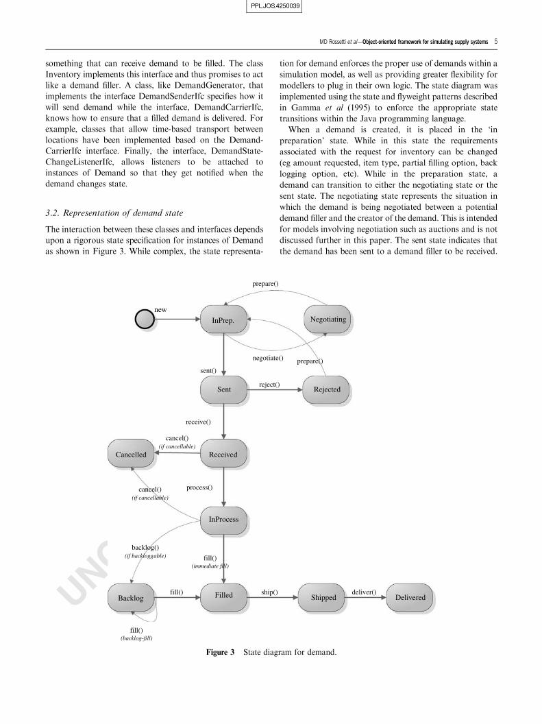
3.2. Representation of demand state

The interaction between these classes and interfaces depends

upon a rigorous state specification for instances of Demand

as shown in Figure 3. While complex, the state representa-

tion for demand enforces the proper use of demands within a

simulation model, as well as providing greater flexibility for

modellers to plug in their own logic. The state diagram was

implemented using the state and flyweight patterns described

in Gamma et al (1995) to enforce the appropriate state

transitions within the Java programming language.

When a demand is created, it is placed in the ‘in

preparation’ state. While in this state the requirements

associated with the request for inventory can be changed

(eg amount requested, item type, partial filling option, back

logging option, etc). While in the preparation state, a

demand can transition to either the negotiating state or the

sent state. The negotiating state represents the situation in

which the demand is being negotiated between a potential

demand filler and the creator of the demand. This is intended

for models involving negotiation such as auctions and is not

discussed further in this paper. The sent state indicates that

the demand has been sent to a demand filler to be received.

PPL_JOS_4250039

prepare()

negotiate()

new

Received

Rejectedreject()

prepare()

InProcess

Filled

sent()

process()

Cancelled

cancel()(if cancellable)

fill()(immediate fill)

Shippedship()

Delivereddeliver()

Backlog

backlog()(if backloggable)

fill()(backlog-fill)

fill()

cancel()(if cancellable)

Sent

receive()

InPrep. Negotiating

Figure 3 State diagram for demand.


UNCORRECTED PROOF

We model the possibility of a time delay in acknowledging

receipt by a demand filler.

From the sent state, the demand can either be placed in

the rejected state or placed in the received state. In our

modelling, demands can be rejected for a number of reasons.

For example, if a demand is sent to a filler that does not

stock the indicated item type, the demand will be rejected.

Or, for example, if a demand that does not allow back-

logging is sent to a filler that permits backlogging but the

demand cannot be immediately filled, the demand will be

rejected. This is like the concept of a lost sale; however, the

burden is placed on the sender of the demand to properly

respond to the rejection. The user can provide preferred

actions to react to the rejection via a listener attached to the

rejection state. For instance, in the case of the ‘lost sale’

rejection, the user could try to find another filler for the

demand or simply tabulate the number of lost sales.

A demand is placed in the received state once a filler has

acknowledged the request. During the receiving, the filler

may indicate what will happen to the demand if the filler is

asked to fill the demand at the current time. For example,

the demand has a status attribute that indicates what might

happen (eg immediate fill, backlog, rejection, etc). Thus,

receiving only acknowledges the demand and sets up the

demand to be filled. Once the demand has been received, it is

up to a listener attached to the demand’s received state to

decide whether or not to proceed with asking the indicated

filler to commit to filling the demand. Thus, from the

received state the demand can either be cancelled or it may

be placed in the process state at the filler. If the demand is

cancelled, the state of the filler never changes. It will be as if

the demand never was sent/received. If the demand is placed

in process at the filler, then this represents a commitment by

the filler to eventually fill the demand’s requirements. For

example, once the demand is placed in process at the filler,

the sender knows ‘for sure’ that the quantity associated with

the item type is on order. While the demand is in process at

the filler, it may still be cancelled or it may be backlogged or

filled. If a demand that allows cancellation is cancelled, it is

placed in the cancelled state, otherwise, an exception is

thrown. A demand that enters the cancelled state will notify

a listener on the demand that it has been cancelled. This

allows the sender to properly react to the cancellation.

If the demand allows backlogging and the filler provides

backlogging, the demand will be placed in the backlogged

state if it cannot be immediately filled in its entirety. While in

the backlogged state, if the demand permits partial filling,

then it can be given increments of the amount requested until

it becomes filled. If it does not allow partial filling, it is up to

the filler to not violate the no partial filling requirement by

only allocating the entire amount needed to the demand

when it becomes available. Once a demand has received all

that it has requested, it is placed in the filled state. A listener

can be attached to the demand’s filled state to initiate

transport once the demand is filled. A demand cannot be

transported until the entire amount that was originally

requested by the demand has been filled. Transport may take

simulated time. Thus, when a demand is placed in the

shipped state, it is considered in transit to its delivery

location. Once it arrives at the delivery location, it must be

placed in the delivered state. A listener can be attached to the

delivered state to react to the delivery of the demand. For

example, once a demand is delivered, the amount filled on

the demand can be used at the delivery location (eg to

replenish inventory on hand).

3.3. Inventory and demand filling

Now that the details of the underlying state transitions for

demand has been covered, we can proceed to the details

about how to fill the demand. The interface, DemandFiller-

Ifc, defines the expectations of a demand filler through its

receive(Demand d ) and fillDemand(Demand d ) methods. A

demand sender will call a demand filler’s receive( ) method

with the demand that it wants the filler to receive. The

receive( ) method places the demand in the received state.

Once the demand has been received (placed in the received

state), a demand sender should call the fillDemand ( ) method

of the filler. The fillDemand ( ) method places the demand in

the ‘in process’ state. The amount requested for the demand

is now ‘on order’ at the filler. In the case that the filler is an

instance of Inventory, the inventory will try to fill the

incoming demand based on its current state. Because the

class Inventory can both fill demands and may send

demands for replenishment, it implements both of the

DemandFillerIfc and the DemandSenderIfc interfaces. In

other words, it acts as both a sender and a filler of demand.

The demand sender interface simply indicates what type of

item the sender may request.

The current state of inventory is represented by four key

variables: amount of inventory on hand (I(t)), the amount

on order (IO(t)), the amount backordered (B(t)), and the

inventory position (IP(t)¼ I(t)þ IO(t)�B(t)). Inventory

must have an inventory control policy attached to govern

when and how much it should order. Whenever any of the

variables constituting the inventory position change, the

inventory policy is notified. It is up to the inventory policy to

appropriately react (or not react) to the change in inventory

position. For example, in the case of continuous review

reorder point policies, the inventory position will be checked

against the reorder point and if it is equal to or below the

reorder point a replenishment demand will be made. In the

case of periodic review, the notification can be ignored since

the inventory position is only checked at the end of review

periods. Note that our design allows the inventory policy to

change during the run and allows the inventory policy

parameters to be updated during the simulation.

Because demand may not necessarily be in units of one,

inventory can handle partial filling if the demand permits

partial filling. In the case of non-single unit demand, the

PPL_JOS_4250039


UNCORRECTED PROOF

filling of backorders can be complicated. For example,

suppose there are demands waiting in the backlog queue for

the following amounts (2, 4, 1, 5), with 5 being the demand

that has been in the queue the longest. Suppose that a

replenishment amount occurs for the quantity 4, how should

the four units be allocated to the waiting orders? Should the

demand waiting for 5 units get 4 of the units and continue

waiting? Should the demand for 4 be given all of the units?

Or, should the demands for 1 and 2 units be filled? Because a

user may want to have complex allocation rules for

processing the backlog queue, the design allows different

backlog policies to be implemented by sub-classing from

BackLogPolicyAbstract. The default backlog policy gives all

the units that it can fill to the demand that has waited the

longest. Note that an instance of Inventory may or may not

have a backlog policy attached. If it does not have a backlog

policy attached, then B(t) will be zero. If it does have a

backlog policy attached, not only is B(t) tabulated, but the

number of demands waiting is also tabulated since the

amount backordered can be different from the number of

demands backordered when demand is not in units of one.

To make the discussion more concrete and to illustrate the

use of the framework, we present the implementation of a

continuous review, reorder point (s), order up to level (S)

model. In this example, an item is managed with (s¼ 3,

S¼ 5). The demand occurs according to a Poisson process

with rate 3.6 per month. The lead time from the supplier to

fill a replenishment order is (0.5) months. We are interested

in estimating the average on hand, average amount back-

ordered, the average amount on order, the fill rate, the

portion of time out of stock, and the number of replenish-

ment orders made.

Exhibit 1 illustrates how simple it is to create a model for

this situation using the framework. First, the item type is

defined. Then, a LeadTimeDemandFiller is created. A

LeadTimeDemandFiller is a class that implements the

DemandFillerIfc and can fill any demand that is sent to it

for its defined item types after a delay that can be stochastic.

It represents the location that will satisfy replenishment

demand for the inventory when inventory reaches its reorder

point. After setting up the supplier, we can define the

inventory by creating its back log policy, its inventory policy,

and telling it to use the instance of LeadTimeDemandFiller

as its supplier. Finally, an instance of a DemandGenerator is

used to create demands and send them to inventory to be

filled. A DemandGenerator acts similarly to the CREATE

block in many common commercial simulation languages.

The user can specify the time between demands as a random

quantity as well as the number of demands to generate, etc.

The demand generator creates instances of Demand, sets

their requirements and then calls its specified filler to request

that the demand be received and then filled.

The simulation was run for 30 replications of 3360 months

with a warm up period of 360 months. The results of the

simulation are given in Table 1. The results are the average,

standard error, 95% half-width, minimum, and maximum

over the 30 replications for each of the performance

measures. These results match the theoretical results for this

simple case. These performance statistics are available as a

standard product of the inventory package and the JSL.

Although a rigorous analysis can be employed to determine

the number of replications and the replication length, we

picked the run-length and warm-up period based on

convenience for the examples within this paper. We did this

because our purpose is to illustrate the modelling, not the

analysis of the results. Despite this intuitive selection of

simulation run parameters, our results can be validated

against the analytical solutions, when appropriate.

PPL_JOS_4250039

Exhibit 1 Simple reorder point, order up to level inventory model.


UNCORRECTED PROOF

Based on the model of Exhibit 1, it should be clear that to

model many item types at a single location, we can simply

repeat the code and build a bigger model. To build on this

idea, we created a class called InventoryHolderAbstract that

facilitates the holding of any number of instances of

Inventory. Instances of concrete sub-classes of Inventory

HolderAbstract then serve as the nodes in a supply chain

(eg Figure 1). In the next section, we discuss the application

of these concepts to supply chain modelling.

4. Supply chain modelling

The class InventoryHolderAbstract represents something

that can hold inventory by item type. Figure 4 is a class

diagram that illustrates the behaviours and attributes of the

classes and the relationship between each of the class that are

used in supply chain modelling.

As shown in the figure, InventoryHolderAbstract is a sub-

class of DemandFillerAbstract, which implements the

DemandFillerIfc interface. Thus, sub-classes of Inventory

HolderAbstract (ie inventory holders) are also demand

fillers. It is also apparent from the figure that Inventory

HolderAbstract acts like a demand sender because it

implements the DemandSenderIfc interface. In fact, both

of these roles are given to an IHP because it holds instances

of inventory. External demands that are sent to an inventory

holder, are essentially routed to the appropriate instance of

inventory in order to be filled. From the outside, sub-classes

of InventoryHolderAbstract are simply demand fillers

(ie something that promises to fill demand). It does not

really matter how the demand requests are filled, only that

they are eventually filled once the fillDemand() method

(behaviour implemented from the DemandFillerIfc) is

called. An inventory holder delegates the demand filling to

the appropriate inventory for the item type associated with

the demand. Thus, the building of a complex supply chain is

a matter of hooking up demand fillers and demand senders

in a similar manner as shown in Exhibit 1 using the

setDemandFiller() method. It is important to note that to

extend this modelling, users simply have to implement the

appropriate interfaces or abstract base classes. Thus, a wider

variety of inventory system modelling than shown here is

very feasible. The next section explains the interactions

between TimeBasedShippingMultiEchelonIHPNetwork,

LeadTimeDemandFiller and TimeBasedDemandCarrier

with the other classes in Figure 4.

4.1. Multi-item, multi-location example

In this section, we illustrate how to model a multi-item,

multi-location supply system as shown in Figure 5. In this

system, there are four different types of items, each of which

can be produced and delivered by an external supplier (eg

manufacturer). The time to produce each of the items may

be stochastic and different as shown in the figure. The time

to transport an item from the factory to the warehouse is set

to 3 days in our example. Table 2 gives the time between

arrivals for the retailers for each of the items as well as the

stocking policies for each of the locations. The transport

time from the warehouse to any of the retailers is 1 day.

An instance of the TimeBasedShippingMultiEchelonI-

HPNetwork class was used to model the example. A multi-

echelon inventory network consists of a network of

InventoryHoldingPoints (IHP), which is a concrete sub-

class of InventoryHolderAbstract. In this type of network,

each IHP can have one parent IHP that fills its replenish-

ment requests. It can have many child IHPs for which it fills

replenishments. No checking is done to ensure that the IHPs

are compatible in terms of their ability to supply certain item

types. Any demands sent to an IHP that cannot be handled

by the IHP will be rejected. The default rejection behaviour

for an IHP is to throw an exception. To override this

behaviour the client can supply a DemandListenerRejecte-

dIfc for the IHP or DemandGenerator. This listener could

have logic that incorporates sense and respond logistics

features into the supply chain. For example, let us consider a

logistic network in a war zone. If the demand filler is

destroyed, then the default behaviour can be overridden to

choose another demand filler based on the current state of

the network.

The top-level supplier is modelled with a LeadTime-

DemandFiller and is considered an external supplier to

the network. The external supplier has an infinite supply of

the item types added to the network, which can be produced

and delivered after a given lead time, which may depend on

PPL_JOS_4250039

Table 1 Results for simple reorder point, order up to level inventory model

Avg. Std error Half-width Min Max

On hand 2.731 0.003 0.006 2.697 2.766On order 1.801 0.003 0.006 1.765 1.836Amount backordered 0.033 0.00029 0.00058 0.029 0.035Backorder waiting time 0.122 0.00065 0.0012 0.115 0.129Fill rate 0.926 0.00056 0.0011 0.912 0.932Out of stock time 0.073 0.00049 0.00096 0.067 0.077Number of replenishments 5404.43 9.301 18.277 5295.0 5509.0


UNCORRECTED PROOF

the item type. Since the top level supplier is external to the

network, the lead time represents the time to produce

the item. If no item types are added, then all demands sent to

the external supplier will be rejected.

The time to transport from the external supplier may

depend on the location of the customer (IHP) (eg warehouse

in the example) and is thus modelled as a separate transport

time which may depend upon the customer and its location

relative to the external supplier. If the time for the transport

depends upon the link between the external supplier and the

customer, then a TimeBasedDemandCarrier is used to

model the transport time from the external supplier to the

top level IHPs. The generation of external demand to

the IHPs is modelled through the use of instances of the

DemandGenerator class. Each IHP may have zero or more

demand generators attached to it, and each DemandGen-

erator may be attached to one or more IHPs. This may occur

for any IHP at any level of the network to represent external

demand sent to that IHP. During the attachment process,

the client is responsible for specifying the time that it may

take to transport the demand to the demand generator once

it is filled. If no demand generators are attached to any

IHP (or to the network) then nothing will happen, since

IHPs must have demands sent to them to begin processing.

In addition, external demand generators may be attached

to the network by calling the allowExternalDemandGenera-

tors() method which allows the IHPs to transport the items

to the external demand generators with zero delay. The

external demand generators must know where to send their

demands (typically through a DemandFillerFinderIfc to

which they have access). The DemandFillerFinderIfc inter-

face defines a general procedure by which a demand filler can

be found for a demand sender. The demand generator in this

example does not use the demand filler finder because we

have attached a demand filler directly to it. However, it is

possible to attach a demand filler finder, which encapsulates

the logic to find a supplier for the demand generator. Thus,

we can easily handle a situation that involves multiple

PPL_JOS_4250039

Figure 4 Key classes and their relationships for supply chain modelling.


UNCORRECTED PROOF

suppliers for a location. It is a simple matter to supply the

logic for choosing between suppliers within the class that

implements the DemandFillerFinderIfc interface. In the

current architecture, if the demand generator has a demand

filler finder attached, it uses the finder to find an appropriate

filler, otherwise, it must have a DemandFillerIfc directly

attached. If no demand filler is attached or a demand filler

finder is not supplied, an exception will be thrown.

Note that the dashed lines and parts in Figure 5 refer to

the information flow upwards in the network with regard to

associated item-requests for replenishments while the solid

shapes imply the actual physical entities that flow downward

in the system.

Exhibit 2 is self-explanatory and illustrates how easily the

components of the system, such as for those retailer 1 and

item type 1 can be built using the classes within the

framework. The other components can be instantiated in a

similar fashion.

The simulation was run for 30 replications of 5400 days

(10 years) with a warm-up period of 1800 days (5 years). A

sample of the simulation results is given in Table 3

(additional descriptive statistics are readily available). These

results represent the aggregate performance for each of the

locations across the item types stocked at the locations. In

addition to these aggregate statistics, which are automati-

cally tabulated, all individual statistics (as per Table 1) for

each item type for each location are readily available. The

numbers in parentheses in the table represent the standard

error.

As one can imagine, for a large network a large amount of

individual and aggregate statistics can be generated. Fill rate,

expected number of back orders, customer wait time are just

PPL_JOS_4250039

Factory

Retailer 1 4reliateR2reliateR Retailer 5Retailer 3

Warehouse

1 2 3 4 1 2 3 4 1 2 3 4 1 2 3 4 1 2 3 4

Production Times

SKU Production TimeItem 1 Expo(1.0)Item 2 Expo(0.5)Item 3 Expo(1.5)Item 4 Expo(2.0)

Warehouse Policies(r,Q) Policy

Item 1 (4,1) SKU

Item 3 (3,2) Item 2 (5,1)

Item 4 (4,2)

Transportation Times

From To DistributionFactoryWarehouse

WarehouseReatilers

Constant(3.0)Constant(1.0)

Figure 5 Multi item multi location example problem.

Table 2 Multi-item multi-location example problem data

Item 1 Item 2 Item 3 Item 4

Retailer 1 TBABexpo(2.0) TBABexpo(1.0) TBABexpo(1.5) TBABexpo(3.0)(s, S)¼ (2, 3) (s, S)¼ (1, 2) (s, S)¼ (2, 4) (s, S)¼ (3, 6)






UNCORRECTED PROOF

some of the operational performance measures that are

relevant to a supply network both at an individual and an

aggregated level. Individual performance refers to a single

item at a particular facility, say fill rate associated with an

item at a particular facility. Aggregated statistics are those

associated across the items at a facility or across the facilities

in the network. The JSL supports the writing of all the

statistics to a database for post processing by the analyst. In

the following section, we present another example model to

illustrate how the framework can be used to model a system

involving the repair of spare parts.

4.3. Multi-echelon spare parts network example

In this section, we describe the modelling of a multi-echelon

spare parts supply system similar to the class of systems

examined via the METRIC (multi-echelon technique for

recoverable item control). For further information on

METRIC, we refer the reader to Sherbrooke (1992) or to

Muckstadt (2005). Since analytical results for METRIC-like

systems exist, our purpose is again expository. The system

can be conceptualized as a set of air bases served by a depot.

The air bases have flying activity that causes spare parts to

be required. Both the depot and the bases, stock inventory

and repair defective parts. Parts that are removed from the

aircraft are called line replaceable units (LRUs). When an

LRU fails on an aircraft at a base, it is removed from an

aircraft and a replacement LRU is withdrawn from

inventory at the base (called base stock). The new part is

placed on the aircraft so that it can continue its operation. If

a replacement part is not available in base supply, a

backorder for the part is issued. The failed part that had

been removed from the aircraft will be either repaired at the

base or at the depot according to a probabilistic process.

There is a chance rij that an LRU of type i will be repaired at

base j. Whenever the failed part is transported to the depot

for repair, a request is made to ship a replacement LRU to

the base. If such a unit is on hand at the depot, then it will be

immediately shipped. If such a unit is not available at the

depot, then a backorder occurs at the depot, which will be

served on a first come first served basis. Figure 6 illustrates

this process. In essence, this system is a multi-echelon system

with one-for-one replenishment (S-1, S) at each location and

the possible lead-time based on repair activity.

The depot and bases in this example stock the inventory

and hence can be constructed using an IHP. However, in this

case, the depot and base also must handle repair activities. In

order to accommodate the repair, we sub-classed the

PPL_JOS_4250039

Exhibit 2 Example code for building the multi-item, multi-location model.

Table 3 Illustrative results for multi-item, multi-location model

R1 R2 R3 R4 R5 W N

On hand 6.35 (0.03) 4.92 (0.03) 4.97 (0.03) 7.77 (0.03) 4.68 (0.03) 0.83 (0.01) 29.52 (0.07)On order 9.13 (0.05) 10.72 (0.05) 7.76 (0.04) 8.19 (0.05) 19.00 (0.07) 60.13 (0.10) 114.93 (0.22)Fill rate 0.53 (0.00) 0.48 (0.00) 0.61 (0.00) 0.54 (0.00) 0.16 (0.00) 0.10 (0.00) 0.27 (0.00)


UNCORRECTED PROOF

InventoryHoldingPoint into InventoryRepairingHolding-

Point. It decides whether the failed part (equivalent to a

demand arrival and demand arrival process equivalent to the

failure process) can be repaired locally and this probability

for each item type is specified and stored within the class.

The repair time distribution for each item type is modelled

using an instance of LeadTimeDemandFiller class within

this class. The repair probability and repair time distribution

for each item are specified by calling the setRepairStation

method of the InventoryRepairingHoldingPoint class.

The simulation model of the METRIC model in Figure 6

was modelled using TimeBasedShippingMultiEchelon-

IHRPNetwork and is similar to TimeBasedShippingMul-

tiEchelonIHPNetwork class which we discussed earlier. Both

of the network building classes are similar except that the

former holds the InventoryRepairingHoldingPoint and the

PPL_JOS_4250039

Figure 6 Multi-echelon spare parts supply system.

Exhibit 3 Example code for building multi-echelon spare parts supply system.


UNCORRECTED PROOF

latter holds InventoryHoldingPoint. The instance in the

Figure 6 was modelled as shown in the Exhibit 3. The

simulation was run for 10 replications of 3650 time period

with a warm up period of 100 time period.

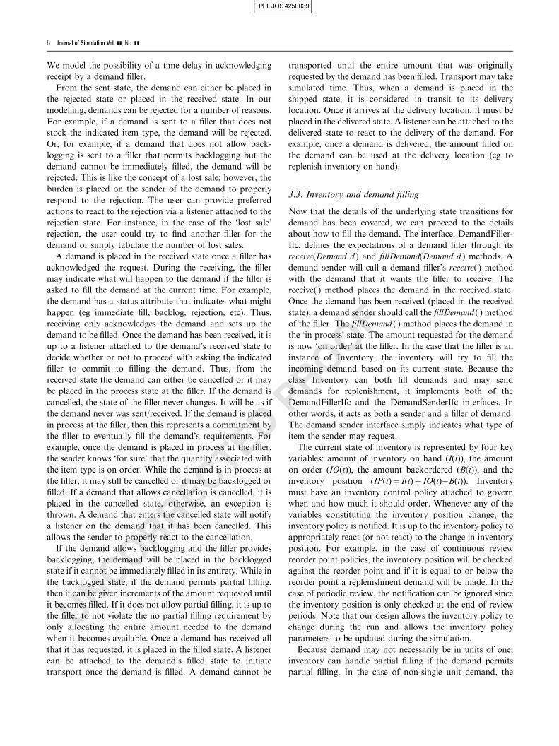
Table 4 tabulates the expected back order and the stock

out frequency from the simulation model (many additional

performance measures are available). The standard error is

negligible (of the order of 4 zeroes) and hence not listed. The

analytical results from the METRIC and VARIMETRIC

computations are listed for comparison. We observe that the

simulation output is within statistical error of the analytical

results.

5. Summary and future research

In this paper, we have introduced and illustrated the use of

an object-oriented framework for simulating supply chains.

We did not provide a complete discussion of all of the

implementation details of all classes in the framework;

instead we provide enough detail on important classes along

with their important behaviours in order to illustrate their

use and functionality through a number of examples. Hence,

the reader can make conceptual modelling with the frame-

work more concrete. In addition, it should be clear that a

variety of complex systems can be modelled where at each

echelon, at each IHP, as well as for each item type a variety

of different inventory policies, backlogging policies, and

demand transport options can be used.

The framework is built upon the JSL, which is an object-

oriented open source framework for simulating within Java.

Because the framework is object-oriented and built on Java,

the modeller can use all the power of the object-oriented

modelling and Java to develop additional models and

behaviours. The JSL is licensed under the GNU General

Purpose License (www.gnu.org). This license is stronger than

the Lesser GPL that is often used for libraries. The use of the

ordinary GPL limits the proprietary use of the JSL and

makes it more readily available to the open-source commu-

nity. Since the JSL is licensed under the GPL and this

framework is based on the JSL, this framework is also

available via the GPL. This makes it a potential valuable

resource for researchers and practitioners working in the

area of supply chain simulation.

We are continuing our modelling efforts on the frame-

work. In particular, we are examining the modelling

of unreliable systems (where the demand filler may be

unavailable), auction based supply/demand situations,

integrating forecasting methods into the supply chain

system, cost modelling, and integrated truck-load or

less-than-truck load transport between locations.

Acknowledgements—This material is based upon work supported bythe US Air Force Office of Sponsored Research and the Air ForceResearch Laboratory. Any opinions, findings, and conclusions orrecommendations expressed in this material are those of the author(s)and do not necessarily reflect the views of the US Air Force.

References

Bagchi S, Buckley SJ and Lin G (1998). Experience using the IBMsupply chain simulator. In: Medeiros DJ, Watson EF, Carson JSand Manivannan MS (eds). Proceedings of the 1999 WinterSimulation Conference. Piscataway, NJ: Institute of Electricaland Electronic Engineers, pp 1387–1394.

Bowersox DJ et al. (1972). Dynamic Simulation of PhysicalDistribution Systems. Division of Research, Graduate Schoolof Business Administration, Michigan State University: EastLansing, MI.

Chatfiled DC, Harrison TP and Hayya JC (2006). SISCO: Anobject-oriented supply chain simulation system. Decis. Supp.Syst. 42(1): 422–434.

Culosi SJ (2001). A simulation for evaluating the operationalreadiness of the supply chain, MacLean, VA. Available throughthe Logistics Management Institute: https://akss.dau.mil/Lists/Software%20Tools/DispForm.aspx?ID¼ 30(accessed 2007).

Dong J, Ding H, Ren C and Wang W (2006). IBM SMARTS-COR—A SCOR based supply chain transformation platformthrough simulation and optimization techniques. In: PerroneLF, Wieland FP, Liu J, Lawson BG, Nicol DM and FujimotoRM (eds). The Proceedings of the 2006 Winter SimulationConference. Institute of Electrical and Electronic Engineers:Piscataway, NJ.

PPL_JOS_4250039

Table 4 Illustrative results for multi-echelon spare parts model

Expected back orders Stock out frequency

METRIC VARIMETRIC Simulation METRIC VARIMETRIC Simulation

Depot 0.3471 0.3472 0.3477 0.4169 0.4169 0.4165

Base1 0.0412 0.0453 0.0452 0.2602 0.2561 0.25622 0.0412 0.0453 0.0453 0.2602 0.2561 0.25643 0.0412 0.0453 0.0451 0.2602 0.2561 0.25634 0.0412 0.0453 0.0454 0.2602 0.2561 0.25645 0.0412 0.0453 0.0452 0.2602 0.2561 0.2567

Q3


UNCORRECTED PROOF

Gamma E, Helm R, Johnson R and Vlissides J (1995). DesignPatterns: Elements of Reusable Object-oriented Software.Addison-Wesley: Reading, MA.

Ingalls RG (1998). The value of simulation in modeling supplychains. In: Medeiros DJ, Watson EF, Carson JS andManivannan MS (eds). Proceedings of the 1998 WinterSimulation Conference. Institute of Electrical and ElectronicEngineers: Piscataway, NJ, pp 1371–1375.

Ingalls RG and Kasales C (1999). CSCAT: The Compaq supplychain analysis tool. In Farrington PA, Black Nembhard H,Sturrock DT, Evans GW (eds). Proceedings of the 1999 WinterSimulation Conference. Institute of Electrical and ElectronicEngineers: Piscataway, NJ, pp 1201–1206.

Jain S (2007). A conceptual framework for supply chain modellingand simulation. Int. J. Simul. Process Modell. 2(3–4): 164–174.

Kleijnen JPC (2005). Supply chain simulation tools and techniques:A survey. Int. J. Simul. Process Modell. 1(1–2): 82–89.

Li Y and Zhao JM (2006). Applying adaptive multi-agent modelingin agile supply chain simulation. Proceedings of the 2006International Conference on Machine Learning and Cybernetics,2006.

Muckstadt JA (2005). Analysis and Algorithms for Service PartsSupply Chains. Springer ScienceþMedia, Inc.

Pundoor G and Herrmann JW (2006). A hierarchical approach tosupply chain simulation modelling using the supply chainoperations reference model. Int. J. Simul. Process Modell.2(3–4): 124–132.

Rossetti MD (2007). JSL: An open-source object-oriented frame-work for discrete-event simulation in Java. Under review inSimulation: Trans. Soc. Model. Simul. Int..

Rossetti MD and Chan HT (2003). A prototype object-orientedsupply chain simulation framework. In: Chick S, Sanchez PJ,

Ferrin D and Morrice DJ (eds). The Proceedings of the 2003Winter Simulation Conference. Institute of Electrical andElectronic Engineers: Piscataway, NJ.

Rossetti MD, Miman M, Varghese V and Xiang YS (2006). Anobject-oriented framework for simulating multi-echelon inven-tory systems. In: Perrone LF, Wieland FP, Liu J, Lawson BG,Nicol DM and Fujimoto RM (eds). The Proceedings of the 2006Winter Simulation Conference. Institute of Electrical andElectronic Engineers: Piscataway, NJ.

Rossetti MD and Thomas S (2006). Object-oriented multi-indenture multi-echelon spare parts supply chain simulationmodel. Int. J. Model. Simul. 26(4).

Schunk D. and Plott B. (2000). Using simulation to analyze supplychain. In Joines JA, Barton RR, Kang K and Fishwick PA(eds). Proceedings of 2000 Winter Simulation Conference.Institute of Electrical and Electronic Engineers: Piscataway,NJ, pp 1095–1099.

Sherbrooke CG (1992). Optimal Inventory Modeling of Systems:Multi-Echelon Techniques. John-Wiley & Sons: New York.

Smiley WA (1997). A logistics simulation and modeling architec-ture. Simulation Interoperability Workshop, Logistics andEnterprise Models Forum, Available at:/http://ms.ie.org/SIW_-LOG/97S/97S-SIW-187.rtfS (accessed: 2007).

Swaminathan JM (1998). Modeling supply chain dynamics:A multi-agent approach. Decis. Sci. 29(3): 607–632.

Systecon (2007). SIMLOX logistics simulation from Systecon[Homepage of Systecon], [Online]. Available: /http://www.systecon.co.uk/products/simlox/S (accessed on 2007).

Received 4 June 2007;accepted 18 December 2007 after two revisions

PPL_JOS_4250039

Q4

Q5

Q6

Q7

Q8

Q9


Documents

An object-oriented framework for simulating supply systems · An object-oriented framework for simulating supply systems MD Rossetti*, M Miman and V Varghese ... to a simulation-based