1

An MPC-based Approach to Provable System-wideSafety and Liveness of Autonomous Ground Traffic

Kyoung-Dae Kim and P. R. Kumar

Abstract—An important area of cyber-physical systems re-search is the development of smart ground transportation systemsdue to their potentially significant impact on safety, the economy,and the environment.

We propose an approach based on Model Predictive Control(MPC) for the development of provably collision free autonomousground transportation systems, and present an autonomous in-tersection management framework. The MPC approach enablesa vehicle to generate its own motion locally in time based on anoptimization framework, incorporating constraints based on thestates of other vehicles in the neighborhood, the speed limit of aroad, the maximum values of acceleration and deceleration, etc.Safety and liveness of the traffic are however system-wide prop-erties, not merely neighborhood properties, and the challenge isto augment this distributed optimization with coordination rulesthat guarantee overall system-wide safety as well as liveness of thetraffic. We design two vehicle-to-vehicle (V2V) coordination rules,along with a vehicle-to-infrastructure rule, and establish thesystem-wide safety and liveness of the autonomous traffic basedon each vehicle’s MPC motion planner, operating in conjunctionwith an algorithm that orders vehicles according to their runtimeproperties. We also conduct a comparative simulation study of thethroughput performance at an intersection of the above approachagainst another popular algorithm, the All-Way STOP.

Index Terms—Safety, Liveness, Autonomous Vehicles, ModelPredictive Control, Motion Planning, Intelligent Intersections.

I. INTRODUCTION

Among others, next generation transportation systems isone of the important application domains of cyber-physicalsystems research [1]. Due to its potentially significant im-pact on safety, energy, and the environment, this area hasbeen drawing increasing attention over the last decade fromacademia, industry, and government. Some examples of recentefforts at development of intelligent transportation systems(ITS) are the ITS Strategic Research Program established in2010 by the United States Department of Transportation [2],the eSafety Initiative of the European Commission to improvesafety and efficiency of transportation systems [3], and theITS Initiative in Japan to resolve problems such as trafficaccidents, traffic congestion, and environmental degradationthrough information and communication technologies [4].

There have also been various research efforts looking yearsor decades into the future. An early example is the California

Kyoung-Dae Kim is with the Department of Electrical and Computer Engi-neering at the University of Denver. e-mail:Kyoung-Dae.Kim@du.edu

P. R. Kumar is with the Department of Electrical and Computer Engineeringat Texas A&M University. e-mail: prk@tamu.edu

This material is based upon work partially supported by NSF under Con-tract Nos. CPS-1232602, CNS-1035378 and CCF-0939370, USARO underContract No. W911NF-08-1-0238, and AFOSR under Contract No. FA9550-13-1-0008.

PATH automated highway system (AHS) program [5] in the1990s. In this project, the four-layer AHS control systemsarchitecture was proposed, and it was demonstrated that bothhighway capacity and safety can be improved by automat-ing highway traffic [6]. In the area of autonomous drivingtechnologies, significant progress has been made since thefirst DARPA Grand Challenge held in 2004. At the DARPAUrban Challenge in 2007, six out of 32 vehicles completed therace and demonstrated the feasibility of autonomous driving inurban environments [7]. In developing such autonomous vehi-cles, it is indeed critical for a vehicle to have the capability togenerate feasible trajectories so that it can move autonomouslyon the road without collision, for which several differentapproaches have been used. An example is a model predictivetrajectory generator [8] developed for Boss, an autonomousvehicle that won the race. Another popular approach formotion planning is to use the well known Rapidly-exploringRandom Tree (RRT) algorithm to generate feasible trajectories[9]. In [10], a Model Predictive Control (MPC) framework isused to develop an active front steering control system so thatan autonomous vehicle can follow a given trajectory even ona slippery road.

The collision avoidance problem for intelligent intersectionshas been recently studied by many researchers. In [11], theproblem of system-wide safety of intersection-crossing trafficis studied. A scheme is proposed that consists of a time-slotallocation intersection-crossing algorithm and an algorithm forupdating failsafe motions of each vehicle. An interesting resultshown in [12] is that it is NP-hard to check membershipin the maximal controlled invariant set which is the largestset of states for which there exists a control that avoidscollisions, and an algorithm is proposed to solve such aproblem approximately. In [13], an intersection is modeled asa hybrid automata with two modes, braking and acceleration ofhuman driver’s driving behavior, and a backward reachable setfrom the states corresponding to an intersection area computedto generate motions for an autonomous vehicle so that itcan avoid collision with other vehicles driven by humans atan intersection. An intersection management scheme that isproposed in [14] is similar to our approach, but there areseveral fundamental differences. For examples, in the schemeproposed in [14], a vehicle approaching an intersection needsto reserve a block of time-space in the intersection to crossthe intersection, whereas, in our case, a vehicle can enter anintersection whenever it is allowed to do so by an intersectionwithout any such a time-space restriction. Furthermore, in ourapproach, the decision for safety within an intersection is madecompletely in the continuous domain while, in [14], it is done

2

in a discretized time and space domain.Motivating our paper is a recent study that shows that the ca-

pacity of existing highway systems can be increased by almost300% when vehicles are equipped with sensors for collisionavoidance, and coordinate with each other [15]. However, weare still at an early stage in the design of a guaranteeably safeand efficient autonomous transportation system. Among themany challenges needing to be addressed, we are particularlyinterested in the problem of achieving system-wide safety andliveness of the overall traffic through an appropriate combi-nation of autonomous driving and inter-vehicle plus vehicle-to-infrastructure coordinations. In particular, the system-widesafety was established for the case of single lane traffic andintersection in [11]. However, that result cannot be easilygeneralized to the case of multi-lane situation in which avehicle’s steering motion also needs to be considered for lanechange. To the best of our knowledge, there has been no priorwork in the literature that addresses the problem of provablesystem-wide safety as well as liveness of autonomous trafficyet in multi-lane situations with intersections.

As an approach to tackle the problem, we propose a motionplanning framework based on Model Predictive Control (MPC)[16]. The MPC approach allows each vehicle to optimize itsmovement locally in time in a distributed manner accordingto any objective that is of interest. It allows the incorporationof vehicular and other constraints into the motion planningproblem. We design constraints for the MPC problem that takeinto account the states of other vehicles or objects on roads,speed limits imposed on roads, each vehicle’s kinematic andkinetic properties, etc. The major challenge is however to showthat the entire resulting system is globally safe as well as liveunder such distributed optimization. To achieve this overar-ching goal, we design policies for vehicle-to-vehicle (V2V)and vehicle-to-infrastructure (V2I) coordination, and proposean overall architecture. The policies for coordination play acritical role in achieving the system-wide safety and livenessproperties while the MPC-based motion planning frameworkensures the safety of a vehicle locally. In our solution, weallow for and address several important scenarios such as lanechanges and stopping. We prove that the resulting automatedintersection management framework, employing simple yet ef-fective intersection management algorithms, achieves system-wide safety and liveness of intersection-crossing traffic.

In Section II, the vehicle model is described. In SectionIII, an MPC framework is formulated for the motion planningproblem and the system-wide safety of single lane traffic isexhibited. This result is generalized in Section IV to traffic ona multi-lane road. A simple vehicle-to-vehicle coordinationrule for yielding is introduced in Section V, and it is shownthat each vehicle on a multi-lane road can complete its lanechange motion in time. In Section VI, we address the designof algorithms for the safety and liveness of traffic at anintersection. Simulation results are presented in Section VII,concluding in Section VIII.

II. DEFINITIONS, NOTATIONS, AND ASSUMPTIONS

For simplicity, we consider a discrete-time unicycle kine-matic model for the motion of a vehicle. The approach we

xt

ytθt

vt

ωt

Fig. 1. A unicycle kinematic vehicle model.

present can be generalized to other dynamic models as well.As shown in Fig. 1, at each time t, a vehicle has a state,xt := (xt, yt, θt)

T capturing its position and orientation in thetwo-dimensional plane, and an input vector ut := (vt, ωt)

T

denoting its speed and steering control, with state equation

xt+h = f(xt,ut), (1)

where h is the sampling period.Let C be the set of vehicles. For c ∈ C, let xt(c), yt(c),

vt(c), and ωt(c) denote the x-axis position, y-axis position,linear velocity, and angular velocity, respectively, of vehiclec at time t. We will suppose that a vehicle’s control input ismaintained constant over the duration of the sampling interval[t, t+h), obeying the following constraints: (i) vt ∈ [0, vmax]and (ii) θt+ωth ∈ [θmin, θmax]. Above, vmax is the maximumpermissible vehicle speed, while θmin and θmax are the mini-mum and maximum permissible values for vehicle orientation.

In our approach we make each vehicle responsible for notcolliding with vehicles in front of it, conforming to well-established traditional practice in non-automated highways.This allows for a more robust system with the follower vehicleadopting a cautious behavior, as well as a distributed approach.Given a vehicle ci behind another vehicle cj , we describe whenthe following vehicle can stop and avoid collision with thelead vehicle, irrespective of the lead vehicle’s actions1. In thesequel, for simplicity, we assume without loss of generalitythat each vehicle is a point vehicle, i.e., it occupies only asingle point in two-dimensional plane. This can be generalized.We say that ci is safe with respect to cj at time t, denoting itby ciStcj , if there exists an admissible sequence of motionsof ci such that, for any admissible sequence of future motionsof cj ,

(i) vt+Kh(ci) = 0 for some K <∞, and(ii) (xt+s(c

i), yt+s(ci)) 6= (xt+s(c

j), yt+s(cj)) for all s ∈

[0,Kh].Under these conditions, we say that ci is in an active safe statewith respect to cj , and that cj is in a passive safe state withrespect to ci. This defines an ordered binary relation on C×C,which we call a safety relation at time t.

In this paper we do not address the issues of sensing andcommunication. They are relegated to separate layers. We only

1While this is a bit conservative, it critically decouples behaviors and makespossible a distributed approach to safety, while also disallowing any solutionthat assumes all vehicles are perfectly coordinated and not error prone.

3

x

y ci cj

Fig. 2. A single lane with traffic.

address the decision making layer for vehicle motion planning,coordination, and intersection management scheme, which isonly a part of the overall architecture for provably system-widesafe and live autonomous ground traffic system. In particular,technical issues related to communication for V2V and V2Icoordination and sensing for traffic environment perceptionare not discussed or addressed any further. Therefore, in ourdiscussion in the sequel, we assume that (i) vehicles and inter-section infrastructure can exchange information without packetdelays and drops, (ii) each vehicle can determine its ownand other surrounding vehicles’ position and motions withouterrors, and (iii) intersection infrastructure can determine eachvehicle’s position without errors within the intersection area.

III. SINGLE LANE TRAFFIC

In this section, we consider the case where all the vehiclesare moving on a single lane as shown in Fig. 2. We call thissystem momentarily safe at time t if, for any ci, cj ∈ C, eitherciStcj or cjStci holds. Finally, we say the system is safe if,for any ci, cj ∈ C, either ciStcj or cjStci holds for all t ≥ 0.

Since there is no need for steering for lane change given thatthere is only a single lane, we consider a simpler kinematicmodel xt+h = f(xt, vt) = xt+vth to represent the longitudi-nal motion of a vehicle, instead of the unicycle model. We willsuppose that there are bounds on the acceleration, amax > 0and amin < 0, for all vehicles.2 Let c0 ∈ C be a vehicle ofinterest on the infinite-length single lane. Also, we define theposition of the car immediately ahead of c0, xt as follows:

xt := minc∈Cxt(c) : xt(c

0) < xt(c). (2)

We begin by considering the constraints on the velocity of avehicle that guarantee its safety. The velocity vt that a vehiclemaintains in the interval [t, t+h) needs to be upper and lowerbounded by vt ≤ vt ≤ vt where

vt := max0, vt−h + aminh, (3)vt := minvmax, vt−h + amaxh, vt, (4)

and vt := (−2amin(xt−xt))1/2 ensures that the vehicle doesnot collide with vehicles ahead of it.

Now, given a current speed v of a vehicle, let tH(v) denotethe shortest time to travel the distance xt − xt, coming to astop after traveling this distance, assuming its feasibility. It

2In general, the acceleration (and deceleration) of a vehicle are a functionof the vehicle speed. Hence, amax (and amin) in our discussion should beunderstood as the maximum out of maximum accelerations (and decelerations)determined by considering the entire vehicle speed range.

v

vt−h

vt

vt

vmax

amin

amin

amax

h 2h

Vt

tL(vt) tH(vt)

τ 0

Fig. 3. A constrained speed trajectory region.

involves the velocity profile

v(τ) =

minvmax, v + amaxτ if 0 ≤ τ < τ ′

v(τ ′) + amin(τ − τ ′) if τ ′ ≤ τ ≤ tH(v),(5)

where τ ′ is determined by the following implicit equation

∆x =

∫ τ ′

0

v(τ)dτ + dMB(v(τ ′)). (6)

Above, dMB(v) := −v2/(2amin) is the minimum stoppingdistance for a vehicle with velocity v, with correspondingstopping time tL(v) := −v/amin.

Let us now define a polyhedron Vt, shown in Fig. 3, withfour of its six vertices at (0, vt), (0, vt), (tL(vt), 0), and(tH(vt), 0). We also define Vkt from Vt by

Vkt := vt+kh|(kh, vt+kh) ∈ Vt. (7)

Finally, given a sampling period h and the speed of a vehicleat time t+ kh, we define dS(vt+kh) by

dS(vt+kh) := dMB(vt+kh) + dh(vt+kh), (8)

wheredh(vt+kh) := vt+khh−

1

2aminh

2. (9)

In the following MPC problem, one can choose any costfunction J of interest. The system is safe irrespective of thechoice of J by virtue of the safety-guaranteeing constraintsthat are described. As one example of J , one could considera quadratic cost (xft − xt+Nh)2 that measures deviation withrespect to a “target” position. Such a target position could,for example, be provided by a higher level route planner thatgenerates a sequence of target positions for a vehicle from itssource to its destination. Our main result of this section is thefollowing:

Theorem 1. Suppose at the initial time, ciS0cj for every pair

ci, cj ∈ C with x0(ci) < x0(cj). Then the single lane system issafe if all vehicles in C move under the following MPC motionplanning control:

4

minv(0:N−1)

J(xt, xft ,v(0:N−1)) (10)

s.t. xt+(k+1)h = f(xt+kh, vt+kh)

xt+(k+1)h ≤ xt − dS(vt+kh)

aminh ≤ ∆vt+kh ≤ amaxhvt+kh ∈ Vkt ,

for all k ∈ 0, · · · , N −1, where N is the length of horizon,v(0:N−1) := vt, · · · , vt+(N−1)h is a sequence of linearmotions, and ∆vt := vt − vt−h.

The proof of the Theorem 1 is based on the followingLemmas proved in the Appendix.

Lemma 1. For given vt−h, xt, and xt at time t, if xt <xt − dS(vt−h), then tH(vt) > tL(vt−h) + h.

Lemma 2. If tH(vt) > tL(vt−h)+h as provided for in Lemma1, then there exists a sequence of speeds vt, · · · , vt+Kh forsome K < ∞ such that, for all k ∈ [0,K], (i) vt+kh ∈ Vkt ,(ii) vt+Kh = 0, and (iii) xt+(k+1)h < xt − dS(vt+kh).

The above two lemmas play critical roles in proving theTheorem 1 because Lemma 1 relates the safety distanceconstraint to the constrained speed trajectory region Vt definedin Fig. 3 and the condition for Vt assumed by the safetydistance constraint, that is tH(vt) > tL(vt−h) + h, in Lemma2 is used to prove the existence of a sequence of speedsthat guarantees the perpetual safety of a vehicle. From thedefinition of the safety relation discussed in Section II and theresult of Lemma 2, it is relatively straightforward to obtainthe following results.

Lemma 3. Given ci, cj ∈ C, let xt := xt(ci), xt := xt(c

j),and vt−h := vτ (ci) over τ ∈ [t − h, t). If xt < xt −dS(vt−h), then there exists an admissible speed sequencevt, · · · , vt+Kh for some K <∞ that satisfies ciStcj .Lemma 4. Given ci, cj ∈ C, suppose ciStcj due to Lemma 3.Then ciSt+hcj under MPC motion plan (10) of ci at time t .

Proof of Theorem 1: Choose any vehicle ci ∈ C at time0. From Lemma 4, ciShcj holds for all cj ∈ C such thatx0(ci) < x0(cj) under the MPC motion plan v0 of ci at time0. Similarly, cjShci holds for a vehicle cj such that x0(cj) <x0(ci). Since ci is arbitrary, the system is momentarily safeat time h. Therefore, by repeating the argument from time hto 2h, and so on, we conclude that the entire system is safeunder MPC motion plans of all vehicles in C.

IV. SAFETY OF MULTI-LANE TRAFFIC

We now address the scenario where the vehicles are movingon a road that has multiple lanes. The significant new issuethat arises is that of lane changing. There are two aspects tothe decision making involved. On the one hand, a vehicle muststay in the lane and move to the next lane while respecting theangular velocity constraints. In addition, a vehicle must staysafe with respect to vehicles not only in its own lane, but alsothose in the other lanes. The former constraints are capturedby constraints in the MPC. The latter is ensured by means of

(xt, yt)

dLdH

θt

ALAH

xt

yt

xt

yt

(xt − xt)

(x+L , y+

L )

(x−L , y−

L ) (x−H , y−

H)

(x+H , y+

H)

ωt−h

vt−h

Fig. 4. Free space in forward direction.

the Lane Change Protocol described below. From a broaderperspective this is an instance of a hybrid control probleminvolving both logical as well continuous variables. We notethe subtle point that in this section we only consider the issueof safety of the motions that are generated; we do not consider“liveness,” which in this context is the issue of whether thevehicle will be able to change its lane. This is considered inthe next section, where we also permit the roadway to end,imposing a bound on the distance within which all maneuversare to be completed with vehicles coming to a stop.

We consider an infinite-length multi-lane system with aset of vehicles C. In the following discussion, we use cj torepresent a vehicle c which is currently moving at lane j.Hence the notation cij will represent a vehicle ci in lane j.For a vehicle c, let `(c) denote the lane it is on. If a vehicleis in the process of changing its lane, we let α(c) denote thelane it is changing to. Another possibility is that a vehicle hasthe intention to change its lane, but has not yet commencedthe lane change maneuver. This may be because the positionsof other vehicles in the system or its own position are not yetconducive to commencing the change. We will say that such avehicle has an intention to change its lane, and denote by β(c)the lane it intends to change to. Recall that c0 is a vehicle ofinterest. Let l0 = `(c0) denote the lane on which c0 is. Wedenote a lane that is m lanes to the left of l0 by l+m, and alane that is m lanes to the right of l0 by l−m.

We will choose the sampling interval h sufficiently smallso that no vehicle can cross a lane completely within a timeinterval of length h, i.e., h < Wl/vmax for all lanes l, whereWl is the width of the lane. We will assume that a vehicleonly makes lane changes between adjacent lanes at any giveninstant. It can change multiple lanes only as a sequence ofsuch single lane changes.

Now, we consider a vehicle c0 ∈ C which is changing itslane from lane 0 to lane m, where m ∈ −1, 0, 1. Noticethat, unlike in the case of single lane traffic, we now need todetermine a region in R2 as shown in Fig. 4, which we willcall “free space,” in which a vehicle can move without havingcollisions with other vehicles on the multi-lane road. Hence,in addition to xt, we determine upper and lower bounds in the

5

y direction for a vehicle changing from lane 0 to lane m:

yt :=

y(l+1 ) if m = 1y(l0) if m = 0,−1,

(11)

yt

:=

y(l0) if m = 0, 1

y(l−1 ) if m = −1.(12)

In the Appendix, we describe how to design constraints Vktand Ωkt , which are the angular analogs of Vkt in Section III,to define feasible trajectories under an MPC formulation.

Now we specify the MPC for the vehicle to generate safety-guaranteed motions on multi-lane traffic:

MPC for Lane Change:

minU(0:N−1)

J(xt,xft ,U(0:N−1)) (13)

s.t. xt+(k+1)h = f(xt+kh,ut+kh)

xt+(k+1)h ≤ xt − dS(vt+kh)

θmin ≤ θt+(k+1)h ≤ θmaxaminh ≤ ∆vt+kh ≤ amaxhvt+kh ∈ Vktωt+kh ∈ Ωkt

for all k ∈ 0, · · · , N − 1, where N is the length of thehorizon, xt is the state of c0 at time t, xft is a possible targetstate of c0 at time t, xt+h = f(xt,ut) is the unicycle vehiclemodel in (1), U(0:N−1) := ut, · · · ,ut+(N−1)h, is the finitesequence of motions for a vehicle c0, and

xt := minc∈C+t

xt(c) , (14)

where C+t is the set of front vehicles which are running at or

changing their lanes to lanes 0 or m and it is formally definedas follows:

C+t := cj ∈ C : (xt(c

0) ≤ xt(cj)) ∧ (15)((j = 0 ∨m) ∨ (α(cj) = 0 ∨m)).

In addition to the above MPC, in the case of lane changes wewill also need to coordinate the movements of vehicles acrosslanes. A vehicle on a multi-lane road cannot change its laneat any arbitrary time. In fact, it is a vehicle’s responsibilityto change its lane only when it is safe to do so and toavoid collision with other vehicles. Hence, we introduce thefollowing Lane Change Protocol that each vehicle on a multi-lane traffic needs to follow.

Lane Change Protocol: Suppose a vehicle c0 intends tochange lanes from 0 to m, where m ∈ −1, 1 at time t.Then, c0 initiates its lane change action from lane 0 to lanem only when its state satisfies the following inequalities:

xt < xt − dS(vt−h), (16)xt > xt + dS(v−t−h), (17)

where xt := maxc∈C−t xt(c), v−t−h := vτ (c) for τ ∈ [t −

h, t), c := argminc∈C−t xt(c), and C−t is the set of behindvehicles which are running at or changing their lanes to lane

m and it is formally defined as follows:

C−t := cj ∈ C : (xt(cj) ≤ xt(c0)) ∧ (18)((j = m) ∨ (α(cj) = m)).

For a given vehicle c0, let us define

C+t (c0) := cj ∈ C \ c0 : xt(c

0) ≤ xt(cj). (19)

The main result of this section is that the above combinationof MPC and Lane Change Protocol guarantees safety.

Theorem 2. Suppose that, for any cj ∈ C, cjS0c holds forall c ∈ C+

0 (cj) due to Lemma 8, i.e, an infinitely long multi-lane system is momentarily safe at time 0. Then it is safeif all vehicles c ∈ C move under the MPC motion planningframework (13) and follow the Lane Change Protocol.

The proof depends on the following lemmas, whose proofsare in the Appendix. First, Lemma 5 below plays a role similarto Lemma 1 for the case of single lane traffic, to relate thesafety distance constraint to the constrained linear and angularspeed trajectory regions Vt and Ωt that are determined by thecurrent vehicle’s state xt. Then Lemma 7 proves the existenceof a sequence of motions ut+kh that satisfies the safety basedon the result in Lemma 5, that is dH < dL. Intuitively, dL isthe maximum-braking distance of a vehicle at its current linearspeed vt, and dH is the maximum driving distance of a vehiclewithout colliding with any vehicles in front in its current laneand also in other lanes when the vehicle continues to movewith its current steering angle.

Lemma 5. Given a vehicle c0 ∈ C at time t, if (i) xt <xt − dS(vt−h) and (ii) [θH−t , θH+

t ] ⊂ [θL−t , θL+t ], then we

have dH > dL where θr±t is as defined in (28) for r ∈ H,L.The following Lemma 6 is used in proving Lemma 7.

Lemma 6. Given a vehicle c0 ∈ C at time t, let D(vt, ωt) bethe Euclidean distance between (xt, yt) and (xt+h, yt+h) ofc0 under the unicycle kinematic vehicle model (1) and an input(vt, ωt) over the time interval [t, t+ h) such that ωt = vt/ρtfor some ρt 6= 0. Then D(vt, ωt) ≤ D(vt, 0) for any ωt 6= 0.

Lemma 7. Given a vehicle c0 ∈ C at time t, if dH >dL, then there exists an admissible sequence of motionsut, · · · ,ut+Kh for some K < ∞ such that, for all k ∈[0,K], (i) vt+kh ∈ Vkt , (ii) ωt+kh ∈ Ωkt , (iii) vt+Kh = 0,(iv) xt+(k+1)h ≤ xt−dS(vt+kh), and (v) yt+(k+1)h ∈ [y

t, yt].

Now, from the results in Lemmas 5 and 7, we can establishthe following perpetual safety result for multi-lane traffic usingthe Lane Change Protocol.

Lemma 8. Suppose a vehicle c0 ∈ C is changing its lanefrom lane 0 to lane m for some m ∈ −1, 0, 1. If c0 satisfies(i) xt < xt − dS(vt−h) and (ii) [θH−t , θH+

t ] ⊂ [θL−t , θL+t ],

then c0Stc for all c ∈ C+t (c0).

Lemma 9. Suppose all vehicles in C follow the Lane ChangeProtocol. Given vehicle c0 ∈ C, if c0Stc holds for anyc ∈ C+

t (c0) due to Lemma 8, then c0St+hc holds for allc ∈ C+

t+h(c0) under the MPC (13) of c0 at time t.

6

Proof of Theorem 2: Choose any c0 ∈ C. Since thesystem is momentarily safe at time 0 by Lemma 8, c0Shcholds under the motion u0 of c0 for any c ∈ C+

h (c0) by Lemma9. Similarly, for any c′ ∈ C \ C+

h (c0), cShc0 holds under themotion u′0 of c′. Notice that, since c0 is arbitrary, the system ismomentarily safe at time h. Therefore, by the same argument,we conclude that the system is safe under the Lane ChangeProtocol and MPC motion plans of all vehicles in C.

V. LIVENESS OF MULTI-LANE TRAFFIC

In the preceding section we have presented conditions thatguarantee safety of lane changes. In this section we addressthe issue of liveness. To understand this, one may note thatin Section IV, for a vehicle to change its lane, it must followthe Lane Change Protocol for safety. Specifically, it shouldsatisfy two inequalities of the protocol, (16) and (17), at thesame time. However, unless there is inter-vehicle coordination,there is no guarantee that these conditions will eventuallybe satisfied when a vehicle has a lane change intention. Asan example, suppose there is a vehicle c wanting to changeits lane to the left. In this situation, it is possible to haveanother vehicle c′ which keeps moving in that left lane at aposition slightly behind c so as to violate (17). Then, vehiclec never gets a chance to change its lane. Hence, to avoid suchundesirable situations, it is important to have an agreementbetween vehicles that ensures their cooperation with each otherto guarantee the liveness property of autonomous driving withrespect to lane change on multi-lane roads.

Besides the inter-vehicle coordination issue, there is yetanother important issue that also needs to be addressed. InSection IV, we considered multi-lane roads which are infinitelylong. However, in practice, roads may end within a finitedistance. One example is a T-intersection. Specifically, whena multi-lane road dead ends at an intersection, then vehicleshave to change their lanes to appropriate target lanes beforethe end of the multi-lane road. Thus we need to ensure that allvehicles can change their lanes successfully before reachingthe end of the road. We will need to develop rules for inter-vehicle coordination that achieve this. Moreover, we anywayneed to address how much driving distance is required for avehicle to successfully complete its lane change.

In Section V-A, we introduce an inter-vehicle coordinationrule for lane change. In Section V-B, we determine the drivingdistance required to guarantee a lane change.

A. Inter-Vehicle Ordering and Yielding for Lane Change

We begin by defining an ordered binary relation for totalordering of vehicles in multi-lane traffic.

Definition 1. The ordered binary relation ≺t⊆ C×C, called aninter-vehicle ordering relation at time t, is defined as follows.Given cj , cj′ ∈ C in multi-lane traffic, cj ≺t cj′ when

1) xt(cj) < xt(cj′), or2) vt(cj) < vt(cj′) when xt(cj) = xt(cj′), or3) j < j′ when vt(cj) = vt(cj′) and xt(cj) = xt(cj′).

Above, when vehicles have the same position and speedin the longitudinal direction along the road, we compare the

lanes on which vehicles are currently running to establish atotal ordering between them. However, it may be noted thatany other criterion can be used instead of the lane numbersas long as vehicles can be totally ordered according to thecriterion.

We now introduce a Yield Protocol, which plays a criticalrole in inter-vehicle coordination for lane change:Yield Protocol: If cj ≺t cj′ and β(cj) = β(c′j), then cj shouldyield to cj′ . By this we mean that cj should reduce its speedso that the following is satisfied for some K <∞.

xt+Kh(cj) < xt+Kh(cj′)− dS(vt+(K−1)h(cj)). (20)

This protocol can be incorporated into the MPC motionplanning framework (13) by defining C+

t in (15) as:

C+t := cj ∈ C+

t (c0) : (j = 0 ∨ α(c0) ∨ β(c0)) ∨(α(cj) = 0 ∨ α(c0) ∨ β(c0)) ∨(β(cj) = 0 ∨ α(c0) ∨ β(c0)), (21)

where C+t (c0) := c ∈ C : c0 ≺t c.

We now prove that the conditions for the Lane ChangeProtocol will eventually be satisfied under this Yield Protocol.

Lemma 10. Suppose cj starts to yield to cj′ at time t. Then,under the Yield Protocol, there exists K < ∞ such that oneof the following inequalities is satisfied.

(i) xt+Kh(cj) < xt+Kh(cj′)− dS(vt+(K−1)h(cj)), or(ii) xt+Kh(cj′) < xt+Kh(cj)− dS(vt+(K−1)h(cj′)).

Proof: For simplicity of notation, we use x(t) := xt(cj),v(t) := vt(cj), x′(t) := xt(cj′), v′(t) := vt(cj′), δx(t) :=x′(t)− x(t), and δv(t) := v′(t)− v(t).

First we consider a case where, for any τ > 0 and anygiven v′(t+ s) over s ∈ [0, τ ], there exists v(t+ s) such that(a) dv(t + s)/ds = amin, (b) v(t + s) ≥ 0, and (c) δx(t +τ) = δx(t) +

∫ τ0v′(t + s) − v(t + s)ds > 0. In this case,

since v(t + s) is decreasing, there exists τ ′ > 0 such thatτ ′ := minτ : v′(t+ s) ≥ v(t+ s) ∀s ≥ τ. Let I(τ ′, τ) :=s ∈ [τ ′, τ ] : v′(t + s) > v(t + s) ≥ 0 for a given τ > τ ′.Then, we have δx(t + τ) = δx(t + τ ′) +

∫ ττ ′δv(t + s)ds =

δx(t+ τ ′) +∫I(τ ′,τ)

δv(t+ s)ds.

Notice that∫I(τ ′,τ)

δv(t+s)ds increases as τ increases. Thisimplies that there exists τ such that δx(t + τ) > M for anyM <∞. Therefore, (i) holds with K := dτ/he.

Next we consider a case where, for a given v′(t+ s), thereexists τ ′ such that τ ′ := minτ : δx(t + τ) = 0, for anyadmissible v(t+ s) over s ∈ [0, τ ′]. Notice that, since δx(t+τ ′) = 0 at time t + τ ′, the inter-vehicle ordering between cjand cj′ at time t + τ ′ must be determined according to thesecond and third properties in Definition 1.

Suppose we have cj ≺t+τ ′ cj′ . Then, since v′(t + τ ′) ≥v(t+ τ ′), for any given v′(t+ τ ′ + s) and any τ ′′ > 0, thereexists v(t + τ ′ + s) such that (a) dv(t + τ ′ + s)/ds = amin,(b) v(t+ τ ′ + s) ≥ 0, and (c) v′(t+ τ ′ + s) ≥ v(t+ τ ′ + s)for s ∈ [0, τ ′′]. Using the same argument as above,

δx(t+ τ ′ + τ ′′) =

∫I(0,τ ′′)

δv(t+ τ ′ + s)ds,

7

where I(0, τ ′′) := s ∈ [0, τ ′′] : v′(t + τ ′ + s) > v(t + τ +s) ≥ 0. If I(0, τ ′′) 6= ∅, then δx(t + τ ′ + τ ′′) > 0 sincev′(t + τ ′ + s) > v(t + τ ′ + s) holds for all s ∈ I(0, τ ′′).Therefore, there exists τ ′′ > 0 such that (i) holds at timet+ τ ′ + τ ′′, where K := d(τ ′ + τ ′′)/he.

For cj′ ≺t+τ ′ cj , one can use the same argument to showthat (ii) holds at time t+ τ ′ + τ ′′ for some τ ′′ > 0.

B. Distance to Complete Lane Change, and Lane ChangeBefore a Dead End

As noted above, in many situations one needs to completea maneuver before a certain point in space. In this section,we consider the situation when the multi-lane road has a deadend. We will call such a multi-lane road a semi-infinitely longmulti-lane road. Let xR be the x-position of the end of asemi-infinitely long multi-lane road R, and let C be a set ofvehicles on R, i.e., xt(c) < xR for all c ∈ C. We considerthe problem when every vehicle in C must stop before theend line of R. Then, xt in (14) for the MPC motion planningframework needs to be redefined as follows:

xt :=

minc∈C+t xt(c) if C+

t 6= ∅xR if C+

t = ∅, (22)

where C+t is as defined in (21).

In the following discussion, we only consider the case wherea vehicle c0 ∈ C changes its lane to the left on a semi-infinitelylong multi-lane road R, i.e., β(c0) = 1; the lane change tothe right is addressed similarly.

Our main result in this section, establishing the liveness oflane change on a multi-lane road under the Lane Change andYield Protocols, is the following.

Theorem 3. Suppose a vehicle c0 in C is on lane 0 at time tand wants to change to lane M on the left. Then, under theLane Change and Yield Protocols, there exists an admissiblesequence of motions ut, · · · ,ut+Kh of c0 for some K <∞ such that (i) c0 can be on lane M at time t + Kh, and(ii) xR ≥ xt+kh for all k ∈ [0,K] if

xR − xt ≥M(dS(vmax) + dC(vmax)

), (23)

wheredC(v) := max

dS(v), LC(ρt)

, (24)

LC(ρt) := 2√Wl(2ρt −Wl)− ρtθt, and ρt is the maximum

out of ρH+t and ρH−t .

The proof of this result depends on the following twolemmas, proved in the Appendix. We have already shown inLemma 10 that the Yield Protocol indeed ensures that a vehiclewanting to change its lane will eventually be able to initiateits lane change action. We need to sharpen this and determinethe maximum travel distance within which it can take place.

Lemma 11. Suppose a vehicle c0 decides to change its lanefrom lane 0 to 1 at time t. Then, under the Yield Protocol, c0

satisfies (16) and (17) in the Lane Change Protocol at timet+ kh, for some k ≥ 0 satisfying xt+kh − xt ≤ dS(vmax).

Consider a vehicle approaching the dead end of its multi-lane road, which needs to change its lane. We need to

determine when the vehicle has to initiate its lane changeaction to ensure that it can complete its lane change actionbefore reaching the end.

Lemma 12. Suppose a vehicle c0 initiates its lane changeaction to the left from lane 0 to lane 1 at time t. If xR −xt ≥ dC(vt−h), then, for any ∆y ∈ (0, 2Wl), there exists asequence of motions ut, · · · ,ut+Kh for some K <∞ suchthat (i) xt+kh ≤ xR for all k ∈ [0,K], (ii) yt+Kh− yt = ∆y,(iii) θt+Kh = 0, and (iv) vt+(K−1)h = 0.

Proof of Theorem 3: Let D(v, v′) := dS(v) + dC(v′).Suppose M = 1. By Lemmas 11 and 12, (i) and (ii) aresatisfied since xR − xt ≥ D(vmax, vmax) ≥ D(vmax, vt−h).

Next consider the case where M = 2. Suppose c0 is on lane1 at time t+K1h for some K1 <∞. Then, a vehicle c0 cansatisfy (i) and (ii) if xR − xt+K1h ≥ D(vmax, vt+(K1−1)h).Notice that c0 can complete its lane change from 0 to1 while satisfying xt+kh − xt ≤ D(vmax, vt−h) forall k ∈ [0,K1] by Lemmas 11 and 12. Then, from(23), xR − xt+K1h ≥ xR − (D(vmax, vt−h) + xt) ≥xR − (D(vmax, vmax) + xt) ≥ D(vmax, vmax). SinceD(vmax, vmax) ≥ D(vmax, vt+(K1−1)h), a vehicle c0 cancomplete its lane change from 1 to 2 at time t + K2h forsome K2 ∈ (K1,∞) while satisfying xR ≥ xt+kh for allk ∈ [0,K2]. We can use the same argument for the case ofM = 2 to show that (i) and (ii) are satisfied when M > 2.

VI. INTERSECTION-CROSSING TRAFFIC

Now we turn to a major problem in autonomous groundtransportation systems: How to ensure that vehicles crossintersections autonomously and safely?

Roughly speaking, there are two different approaches toachieving this. The first approach is to let vehicles within an in-tersection area communicate and coordinate by themselves todecide which vehicles are allowed, and when they are allowed,to enter and cross an intersection. Thereby, no additionalinfrastructure would be required for the intersection-crossingtraffic management in this approach. However, it is in generala hard problem to reach such an agreement between manyvehicles at runtime, and, furthermore, this approach wouldrequire a large volume of information exchanges betweenvehicles to reach an agreement to cross an intersection.

Instead, in this paper, we follow an alternative approachwhere there exists an intersection infrastructure to managethe intersection-crossing traffic. In this approach, vehicles arestill responsible for safety while moving along a lane asthey approach and cross the intersection, which is a problemthat has already been addressed in Sections III, IV and V.On the other hand, we delegate to the intersection itself theproblem of coordinating (or ordering) vehicles to ensure theycross the intersection in a safe and live manner. Thus ourarchitecture employs vehicle-to-infrastructure communication.The important challenge in this approach is to integrate thedecisions made by each vehicle in the continuous domain forautonomous driving with the discrete decisions made by anintersection for safe intersection-crossing. Another importantissue is that when a vehicle exits an intersection, it enters

8

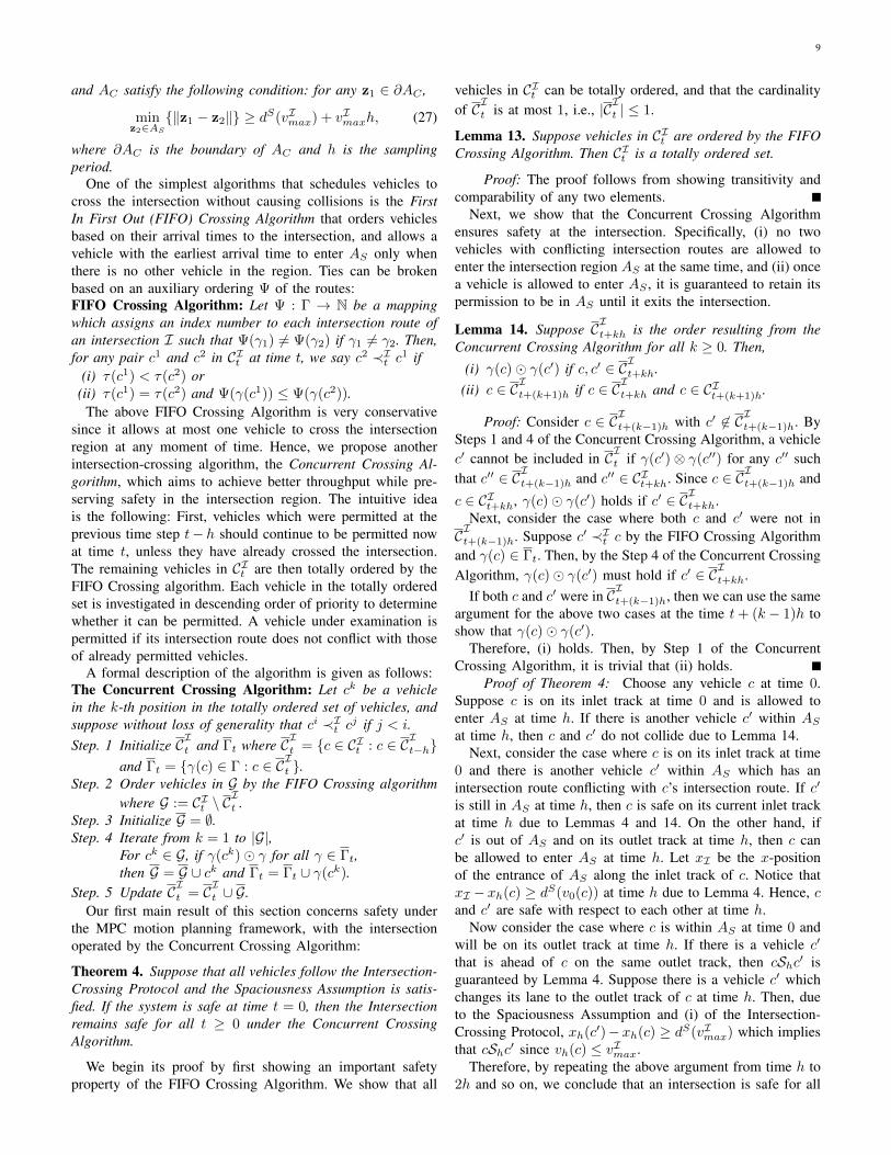
Inlet! Outlet!

(rb, l1)

(rb, l2)

(rc, l2) (rc, l1)

(rd, l1)(rd, l2)

Comm.!Region! Intersec3on!Region!

(ra, l1)

(ra, l2)

Fig. 5. An Intersection with four inlet tracks and four outlet tracks.

a new driving environment, perhaps a multi-lane road. Wewill need to ensure that the vehicle can merge safely intothe that environment. There is a tension in that on the onehand a vehicle needs to expeditiously clear the intersection,while at the same time it has to maintain safety in thepost-intersection environment. In fact, there are several otherchallenging aspects to intersection crossing. When conflictsarise due to vehicles needing to cross each others’ tracks, theywill need to be priority ordered. However, this priority orderingalso needs to not violate any other safety consideration withrespect any other vehicles. To address this challenge, wepropose a framework for autonomous intersection-crossingconsisting of a rule for vehicle-to-intersection coordinationwhich enables seamless interaction between the continuousand discrete domains. It results in algorithms for orderingvehicles at an intersection that guarantee safety as well asliveness.

We begin by defining the constituents of an intersection. LetR := (r, l1, · · · , lm) be a a multi-lane road where r is thename of R, and l1, . . . , lm is the set of lanes constitutingR. We also define a track, denoted by w := (r, l,Wl), whichis the pair consisting of the road name r, the lane number l,and the width of the lane Wl.

An intersection I consists of the following elements:(i) AS , the intersection region which is shared by the roads

connected to the intersection,(ii) AC , the communication region in which vehicles ex-

change information with the intersection,(iii) A set of tracks I and O corresponding to the inlets and

the outlets of the intersection, respectively, and(iv) Γ, a set of intersection routes which connect each inlet

to an outlet of the intersection.Consider a set of vehicles within AC . For each vehicle c ∈

C, the intersection I maintains information about c such asits (i) inlet track, (ii) outlet track, (iii) current position withinAC , and (iv) arrival time to I (more precisely, the time at

which c enters into AC). We denote the vehicle’s inlet trackby i(c), the outlet track by o(c), its position by p(c) ∈ R2, itsarrival time to I by τ(c), and its intersection route by γ(c).Notice that an intersection is an area within AS that connectsfrom the inlet track to outlet track. As an example, the graycolored area in Fig. 9 represents an intersection route from theinlet track (ra, l1) to the outlet track (rc, l1). In the followingdiscussion, we define the arrival time τ(c) of a vehicle c asthe time at which c enters into Ac of an intersection I. Also,we use CIt to represent the set of vehicles in C which stillneed to cross the intersection areas, i.e.,

CIt := c ∈ C : (τ(c) ≤ t) ∧ (p(c) 6∈ Region of o(c)), (25)

where the region of a track is defined as the area within anintersection occupied by the lane associated with the track.

If two intersection routes γ1 and γ2 are intersect, i.e., (γ1)∩(γ2) 6= ∅, then we say that they are in conflict with each other.Above (γ) is the interior of γ. For simplicity of notation, wewrite γ1⊗γ2 if two intersection routes γ1 and γ2 conflict, andγ1γ2 if they do not conflict. Also, we use Γt to denote the setof occupied routes at time t, where we say that an intersectionroute γ is occupied at time t if there exists a vehicle c ∈ CItwith γ(c) = γ where CIt is as defined in (26).

Now we define a vehicle ordering relation, called theintersection-crossing ordering relation, to prioritize vehicleswithin an intersection based on some criteria, and also intro-duce a rule for vehicle-to-intersection coordination, called theIntersection-Crossing (IC) Protocol.

Definition 2. Let ≺It ⊆ CIt × CIt be a binary orderingrelation between vehicles in CIt , called an intersection-crossingordering relation. The specific orderings between vehicles inCIt are determined by some intersection-crossing algorithmswhich are discussed below.

Intersection-Crossing Protocol: Let c be an incoming vehicleto an intersection I with intent to cross the intersection regionAS .

(i) If c is within AC , c does not change its lane.(ii) If c does not have a permission from I to cross the

intersection region AS , c stops before entering AS .(iii) I gives a permission to the vehicles in

CIt := c ∈ CIt : @c′ ∈ CIt s.t. c ≺It c′ (26)

which is the set of vehicles that are maximal in CItaccording to the intersection-crossing ordering relation.

Let us now consider a case when a permitted vehicle c is inthe intersection region AS . Then, upon exiting AS , vehiclec enters into a different driving environment, a multi-lanesystem, in which other vehicles in other adjacent outlet trackscan change their lanes to c’s outlet track or vice versa. Hence,to ensure safety between vehicles on their outlet tracks aftercrossing AS , it is necessary to satisfy the inequalities in theLane Change Protocol. For this purpose, we introduce thefollowing assumption on the intersection.The Spaciousness Assumption: With vImax denoting themaximum speed constraint within AS , we assume that AS

9

and AC satisfy the following condition: for any z1 ∈ ∂AC ,

minz2∈AS

‖z1 − z2‖ ≥ dS(vImax) + vImaxh, (27)

where ∂AC is the boundary of AC and h is the samplingperiod.

One of the simplest algorithms that schedules vehicles tocross the intersection without causing collisions is the FirstIn First Out (FIFO) Crossing Algorithm that orders vehiclesbased on their arrival times to the intersection, and allows avehicle with the earliest arrival time to enter AS only whenthere is no other vehicle in the region. Ties can be brokenbased on an auxiliary ordering Ψ of the routes:FIFO Crossing Algorithm: Let Ψ : Γ → N be a mappingwhich assigns an index number to each intersection route ofan intersection I such that Ψ(γ1) 6= Ψ(γ2) if γ1 6= γ2. Then,for any pair c1 and c2 in CIt at time t, we say c2 ≺It c1 if

(i) τ(c1) < τ(c2) or(ii) τ(c1) = τ(c2) and Ψ(γ(c1)) ≤ Ψ(γ(c2)).

The above FIFO Crossing Algorithm is very conservativesince it allows at most one vehicle to cross the intersectionregion at any moment of time. Hence, we propose anotherintersection-crossing algorithm, the Concurrent Crossing Al-gorithm, which aims to achieve better throughput while pre-serving safety in the intersection region. The intuitive ideais the following: First, vehicles which were permitted at theprevious time step t− h should continue to be permitted nowat time t, unless they have already crossed the intersection.The remaining vehicles in CIt are then totally ordered by theFIFO Crossing algorithm. Each vehicle in the totally orderedset is investigated in descending order of priority to determinewhether it can be permitted. A vehicle under examination ispermitted if its intersection route does not conflict with thoseof already permitted vehicles.

A formal description of the algorithm is given as follows:The Concurrent Crossing Algorithm: Let ck be a vehiclein the k-th position in the totally ordered set of vehicles, andsuppose without loss of generality that ci ≺It cj if j < i.Step. 1 Initialize CIt and Γt where CIt = c ∈ CIt : c ∈ CIt−h

and Γt = γ(c) ∈ Γ : c ∈ CIt .Step. 2 Order vehicles in G by the FIFO Crossing algorithm

where G := CIt \ CIt .

Step. 3 Initialize G = ∅.Step. 4 Iterate from k = 1 to |G|,

For ck ∈ G, if γ(ck) γ for all γ ∈ Γt,then G = G ∪ ck and Γt = Γt ∪ γ(ck).

Step. 5 Update CIt = CIt ∪ G.Our first main result of this section concerns safety under

the MPC motion planning framework, with the intersectionoperated by the Concurrent Crossing Algorithm:

Theorem 4. Suppose that all vehicles follow the Intersection-Crossing Protocol and the Spaciousness Assumption is satis-fied. If the system is safe at time t = 0, then the Intersectionremains safe for all t ≥ 0 under the Concurrent CrossingAlgorithm.

We begin its proof by first showing an important safetyproperty of the FIFO Crossing Algorithm. We show that all

vehicles in CIt can be totally ordered, and that the cardinalityof CIt is at most 1, i.e., |CIt | ≤ 1.

Lemma 13. Suppose vehicles in CIt are ordered by the FIFOCrossing Algorithm. Then CIt is a totally ordered set.

Proof: The proof follows from showing transitivity andcomparability of any two elements.

Next, we show that the Concurrent Crossing Algorithmensures safety at the intersection. Specifically, (i) no twovehicles with conflicting intersection routes are allowed toenter the intersection region AS at the same time, and (ii) oncea vehicle is allowed to enter AS , it is guaranteed to retain itspermission to be in AS until it exits the intersection.

Lemma 14. Suppose CIt+kh is the order resulting from theConcurrent Crossing Algorithm for all k ≥ 0. Then,

(i) γ(c) γ(c′) if c, c′ ∈ CIt+kh.(ii) c ∈ CIt+(k+1)h if c ∈ CIt+kh and c ∈ CIt+(k+1)h.

Proof: Consider c ∈ CIt+(k−1)h with c′ 6∈ CIt+(k−1)h. BySteps 1 and 4 of the Concurrent Crossing Algorithm, a vehiclec′ cannot be included in CIt if γ(c′)⊗ γ(c′′) for any c′′ suchthat c′′ ∈ CIt+(k−1)h and c′′ ∈ CIt+kh. Since c ∈ CIt+(k−1)h and

c ∈ CIt+kh, γ(c) γ(c′) holds if c′ ∈ CIt+kh.Next, consider the case where both c and c′ were not in

CIt+(k−1)h. Suppose c′ ≺It c by the FIFO Crossing Algorithmand γ(c) ∈ Γt. Then, by the Step 4 of the Concurrent CrossingAlgorithm, γ(c) γ(c′) must hold if c′ ∈ CIt+kh.

If both c and c′ were in CIt+(k−1)h, then we can use the sameargument for the above two cases at the time t+ (k − 1)h toshow that γ(c) γ(c′).

Therefore, (i) holds. Then, by Step 1 of the ConcurrentCrossing Algorithm, it is trivial that (ii) holds.

Proof of Theorem 4: Choose any vehicle c at time 0.Suppose c is on its inlet track at time 0 and is allowed toenter AS at time h. If there is another vehicle c′ within ASat time h, then c and c′ do not collide due to Lemma 14.

Next, consider the case where c is on its inlet track at time0 and there is another vehicle c′ within AS which has anintersection route conflicting with c’s intersection route. If c′

is still in AS at time h, then c is safe on its current inlet trackat time h due to Lemmas 4 and 14. On the other hand, ifc′ is out of AS and on its outlet track at time h, then c canbe allowed to enter AS at time h. Let xI be the x-positionof the entrance of AS along the inlet track of c. Notice thatxI − xh(c) ≥ dS(v0(c)) at time h due to Lemma 4. Hence, cand c′ are safe with respect to each other at time h.

Now consider the case where c is within AS at time 0 andwill be on its outlet track at time h. If there is a vehicle c′

that is ahead of c on the same outlet track, then cShc′ isguaranteed by Lemma 4. Suppose there is a vehicle c′ whichchanges its lane to the outlet track of c at time h. Then, dueto the Spaciousness Assumption and (i) of the Intersection-Crossing Protocol, xh(c′)−xh(c) ≥ dS(vImax) which impliesthat cShc′ since vh(c) ≤ vImax.

Therefore, by repeating the above argument from time h to2h and so on, we conclude that an intersection is safe for all

10

t ≥ 0 if it is safe at t = 0 under the Spaciousness Assumptionand the Intersection-Crossing Protocol.

The above result addresses safety, and now we establish thenext crucial property of the Concurrent Crossing Algorithm,the liveness of intersection-crossing. To do this we needto introduce the following assumption that vehicles exit theintersection and do not loiter:The No Loitering Assumption: If a vehicle c ∈ CIt , thenc 6∈ CIt+Kh for some K <∞. In other words, if c ∈ CIt , thenc will eventually cross the AS region of an intersection I andbe on its outlet track.

It is important to notice that, within the proposed MPCmotion planning framework, this assumption is easily satifiedby choosing the target state xft for the MPC appropriatelyalong the vehicle’s intersection route and outlet track. Themain reason that we need this assumption is to exclude somesituations such as mechanical breakdown of a car, an accidentwith unknown objects in the middle of an intersection, etc.,which cannot be handled via the proposed framework.

Theorem 5. Suppose CIt+kh is determined by the ConcurrentCrossing Algorithm for all k ≥ 0. Let c be a vehicle in CIt suchthat c 6∈ CIt and c ≺It c for any other vehicle c ∈ CIt \ C

It by

the FIFO Crossing Algorithm. Then, under the No LoiteringAssumption, there exists K <∞ such that c ∈ CIt+Kh at timet+Kh.

Proof: Let Gt+kh := CIt+kh \CIt+kh be the set of vehicles

at time t+kh constructed at Step 2 in the Concurrent CrossingAlgorithm. Then, from the hypothesis, c ∈ Gt and c ≺It c forall c ∈ Gt \ c. From the FIFO Crossing Algorithm, this in turnimplies that τ(c) ≤ τ(c) for all c ∈ Gt. Now, suppose there isa new vehicle c′ that is entering into AC at time t+ kh. It isclear that τ(c) < τ(c′).

First, consider the case where c′ ∈ CIt+kh by the ConcurrentCrossing Algorithm. Notice that, at Step 2 in the ConcurrentCrossing Algorithm, c′ ∈ Gt+kh and moreover c′ ≺It+kh c forany c ∈ Gt+kh \ c′ by the FIFO Crossing Algorithm. Hence,from Step 4 in the Concurrent Crossing Algorithm, c′ can beincluded in CIt+kh only when c′ satisfies γ(c′) γ(c) for anyc ∈ CIt+kh \ c′. Thus, γ(c) γ(c′) in this case.

Next, consider the case where c′ 6∈ CIt+kh by the ConcurrentCrossing Algorithm. Since τ(c) < τ(c′), c′ ≺It+kh c by theFIFO Crossing Algorithm. Notice that, if γ(c′) ⊗ γ(c), thenc′ ≺It+kh c holds within Gt+kh for all k < K until c ∈ CIt+Khfor some K <∞ by the Concurrent Crossing Algorithm.

Now, let Gt+kh := c ∈ Gt+kh : (c ≺It+kh c) ∧ (γ(c) ⊗γ(c)). Then, from the above argument and the No LoiteringAssumption, we conclude that there exists k′ such that k < k′

and Gt+k′h ⊂ Gt+kh. Since |Gt| is finite, Gt+Kh = 0 for someK <∞. Therefore, there exists K <∞ such that c ∈ CIt+Kh.

VII. SIMULATION RESULTS

We present simulation results demonstrating system-widesafety and liveness of autonomous ground traffic enabledby the proposed autonomous driving framework consisting

TABLE IPARAMETERS AND THEIR VALUES USED IN SIMULATION.

Parameter Values

Max. Speed (vmax) 27.8m/sec

Max. Acceleration (amax) 3.8m/sec2

Min. Aecceleration (amin) −7.9m/sec2

Sample Period (h) 0.01sec.

Vehicle Length / Width 4.5m/1.7m

Lane Width 3.6m

Min. Turning Radius (ρmin) 5.3m

L0

Fig. 6. The vehicle configuration for the multi-lane traffic simulation, whereL0 := dS(v0) and v0 is the initial speed of a vehicle.

of the MPC-based motion planner, the Lane Change Proto-col, the Yield Protocol, the Intersection-Crossing Protocol,and the Intersection-Crossing Algorithms. We also comparethe throughput performance on an intersection of severalintersection-crossing algorithms. Table I shows the parametervalues used.

A. Multi-Lane Traffic

As an example of multi-lane traffic, consider a multi-laneroad with three lanes. There are six vehicles positioned on theroad, shown in Fig. 6, set to move at the same speed at theinitial time of simulation. Each vehicle has a target lane whichit should eventually reach, randomly chosen out of the threelanes, for each vehicle in the beginning of simulation. Once atarget lane is chosen, the target state xft = (xft , y

ft , θ

ft ) of a

vehicle can be determined by setting xft to the x-coordinate ofthe target position along the road, yft to the y-coordinate of thetarget lane’s center line, and θft to zero. Then a vehicle starts tomove by the motions generated by the proposed MPC motionplanner to reach the given target state xft . At each time stept, each vehicle computes xt and (yt, yt) to determine its freespace and checks whether it can initiate its lane change motionusing the two inequality conditions in (16, 17). If the vehicle’scurrent state satisfies the conditions, then it can proceed tomove to the target lane. However, if any of these conditionsis not satisfied, then the vehicle coordinates its motion withits surrounding vehicles according to the Yield Protocol.

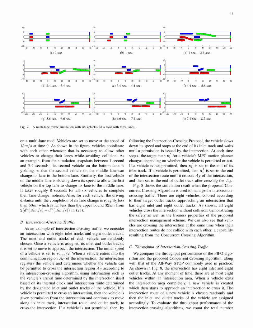
Fig. 7 shows a simulation result which demonstrates thesafety and liveness of the proposed MPC motion planningframework orchestrated with the Lane Change Protocol and theYield Protocol developed for cooperative autonomous driving

11

−30 −20 −10 0 10 20 30 40 50 60−10

−5

0

5

10

(a) 0 sec.−30 −20 −10 0 10 20 30 40 50 60

−10

−5

0

5

10

(b) 1 sec.

−30 −20 −10 0 10 20 30 40 50 60−10

−5

0

5

10

(c) 1 sec. – 2.4 sec.

−30 −20 −10 0 10 20 30 40 50 60−10

−5

0

5

10

(d) 2.4 sec. – 3.4 sec.

−30 −20 −10 0 10 20 30 40 50 60−10

−5

0

5

10

(e) 3.4 sec. – 4.4 sec.

−30 −20 −10 0 10 20 30 40 50 60−10

−5

0

5

10

(f) 4.4 sec. – 5.6 sec.

−30 −20 −10 0 10 20 30 40 50 60−10

−5

0

5

10

(g) 5.6 sec. – 6.6 sec.

−30 −20 −10 0 10 20 30 40 50 60−10

−5

0

5

10

(h) 6.6 sec. – 7.4 sec.−30 −20 −10 0 10 20 30 40 50 60

−10

−5

0

5

10

(i) 7.4 sec. – 8.2 sec.

Fig. 7. A multi-lane traffic simulation with six vehicles on a road with three lanes.

on a multi-lane road. Vehicles are set to move at the speed of15m/s at time 0. As shown in the figure, vehicles coordinatewith each other whenever that is necessary to allow othervehicles to change their lanes while avoiding collision. Asan example, from the simulation snapshots between 1 secondand 2.4 seconds, the second vehicle on the bottom lane isyielding so that the second vehicle on the middle lane canchange its lane to the bottom lane. Similarly, the first vehicleon the middle lane is slowing down its speed to allow the firstvehicle on the top lane to change its lane to the middle lane.It takes roughly 8 seconds for all six vehicles to completetheir lane change motions. Also, for each vehicle, the drivingdistance until the completion of its lane change is roughly lessthan 60m, which is far less than the upper bound 325m from2(dS(15m/s) + dC(15m/s)) in (23).

B. Intersection-Crossing Traffic

As an example of intersection-crossing traffic, we consideran intersection with eight inlet tracks and eight outlet tracks.The inlet and outlet tracks of each vehicle are randomlychosen. Once a vehicle is assigned its inlet and outlet tracks,it is set to move to approach the intersection. The initial speedof a vehicle is set to vmax/2. When a vehicle enters into thecommunication region AC of the intersection, the intersectionregisters the vehicle and determines whether the vehicle canbe permitted to cross the intersection region AS according toits intersection-crossing algorithm, using information such asthe vehicle’s arrival time determined by the intersection itselfbased on its internal clock and intersection route determinedby the designated inlet and outlet tracks of the vehicle. If avehicle is permitted to cross an intersection, then the vehicle isgiven permission from the intersection and continues to movealong its inlet track, intersection route, and outlet track, tocross the intersection. If a vehicle is not permitted, then, by

following the Intersection-Crossing Protocol, the vehicle slowsdown its speed and stops at the end of its inlet track and waitsuntil a permission is issued by the intersection. At each timestep t, the target state xft for a vehicle’s MPC motion plannerchanges depending on whether the vehicle is permitted or not.If a vehicle is not permitted, then xft is set to the end of itsinlet track. If a vehicle is permitted, then xft is set to the endof the intersection route until it crosses AS of the intersection,and then set to the end of outlet track after crossing the AS .

Fig. 8 shows the simulation result when the proposed Con-current Crossing Algorithm is used to manage the intersection-crossing traffic. There are eight vehicles, colored accordingto their target outlet tracks, approaching an intersection thathas eight inlet and eight outlet tracks. As shown, all eightvehicles cross the intersection without collision, demonstratingthe safety as well as the liveness properties of the proposedintersection management scheme. We can also see that vehi-cles are crossing the intersection at the same time when theirintersection routes do not collide with each other, a capabilityresulting from the Concurrent Crossing Algorithm.

C. Throughput of Intersection-Crossing Traffic

We compare the throughput performance of the FIFO algo-rithm and the proposed Concurrent Crossing algorithm, alongwith that of the All-Way STOP commonly used in practice.As shown in Fig. 8, the intersection has eight inlet and eightoutlet tracks. At any moment of time, there are at most eightvehicles within an intersection area. When a vehicle exitsthe intersection area completely, a new vehicle is createdwhich then starts to approach an intersection to cross it. Theintersection route of a new vehicle is chosen randomly andthen the inlet and outlet tracks of the vehicle are assignedaccordingly. To evaluate the throughput performance of theintersection-crossing algorithms, we count the total number

12

(a) 0 sec. (b) 1 sec. (c) 1 sec. – 2.5 sec.

(d) 2.5 sec. – 8.5 sec. (e) 8.5 sec. – 13.5 sec. (f) 13.5 sec. – 19 sec.

Fig. 8. An intersection-crossing traffic simulation with the proposed Concurrent Crossing Algorithm. (At t = 0, eight vehicles are approaching to anintersection at the same speed vmax/2.)

1 2 30

20

40

60

80

100

120

Tota

l Num

ber o

f Car

s Cr

osse

d fo

r 300

sec

Algorithms

STOPFIFO

CON

1 2 30

5

10

15

20

25

30

35

40

45

50

Mea

n of

Inte

rsec

tion−

Cros

sing

Tim

e (s

ec)

Algorithms

STOPFIFO

CON

Fig. 9. A statistical result of an intersection-crossing traffic during 300seconds.

of vehicles crossing the intersection in 300 seconds, and alsomeasure the time taken by each vehicle from its arrival to itsexit from the AC region of the intersection. As shown by theresults in Fig. 9, the proposed Concurrent Crossing Algorithmperforms better than the other two algorithms.

VIII. CONCLUDING REMARKS

We have developed a theoretical framework for collision-free autonomous ground traffic. Specifically, we have for-mulated a Model Predictive Control problem to dynamicallygenerate a feasible sequence of driving motions for a vehiclewhich enables it to avoid collisions with other vehicles.

We have exhibited constraints that guarantee collision-freeautonomous driving by considering the driving states of othervehicles, vehicle-dependent properties such as maximum ac-celeration and deceleration of a vehicle, and driving conditionssuch as the speed limit and the number of lanes on byeach road. Furthermore, to achieve system-wide safety, i.e.,collision-freeness, as well as liveness of the overall traffic,we have proposed vehicle-to-vehicle (V2V) coordination rules,a Lane Change Protocol and a Yield Protocol, which ensureautonomous coordination between vehicles driving on multi-lane roads.

The system-wide safety and liveness of intersection crossingare achieved through a vehicle-to-infrastructure (V2I) coor-dination rule, the Intersection-Crossing Protocol, integratedwith an algorithm that can manage all vehicles while cross-ing the intersection area. We have considered two algo-rithms, a simple FIFO Crossing algorithm and a new andmore performance-oriented Concurrent Crossing algorithm,and shown the system-wide safety and liveness of autonomousintersection-crossing traffic under the proposed intersection-crossing framework.

The proposed theory for autonomous ground traffic is con-servative to some extent, perhaps desirably so. In particular,the constraint in (13), designed for safety of a vehicle withrespect to vehicles ahead of it, is based on a vehicle’s staticview about the motion of other vehicles in ahead of it and thisresults in a greater inter-vehicle separation distance. However,

13

in practice, no vehicle can make an immediate stop due to itsdynamics, as discussed in Section III. Hence, the minimuminter-vehicle distance at a speed v in order to avoid collisioncan be shorter than the proposed maximum-braking distancedS(v), indicating that it is practically possible to have lessconservative results. It is an important issue for future workto redesign constraints for less conservativeness, incorporatethem into the proposed Model Predictive Control framework,and show that the safety is still guaranteed.

As intended by its design, and as shown in the simula-tions, the proposed Concurrent Crossing algorithm performsbetter than the other two algorithms in terms of throughputperformance. However, it is still a conservative algorithmsince no two vehicles are simultaneously allowed to enterinto an intersection area if their intersection routes conflict.As an example, if we consider a case with two vehiclesapproaching to an intersection on the same inlet track andhaving the same intersection route, then under the ConcurrentCrossing algorithm the following vehicle must wait until theleading vehicle crosses the intersection region completely,even though it can cross the intersection without being delayedby following the leading vehicle at the same speed of thevehicle. At the intersection considered in Section VII, thedelay time for this case caused by the Concurrent Crossingalgorithm is at least (4 ×Wl)/v

Imax, whereas the delay can

be zero in an optimal policy. Therefore, it is indeed of greatinterest to develop less conservative and better performingintersection-crossing algorithms.

In the proposed theoretical framework, interactions betweenvehicles and vehicle-to-intersection infrastructure are criticalfor achieving system-wide safety and liveness. In this paper,we assume for such interactions that (i) the driving statessuch as position and speed of a vehicle in the vicinity ofan entity, i.e., a vehicle or an intersection, can be measuredby the entity without error, and (ii) the information suchas lane change intention, lane change action, and also theinlet-outlet tracks for intersection-crossing can be exchangedwithout having any packet delay and loss. It is an importantdirection of research in the future to relax these assumptionsso that the proposed framework can be applicable in practicewhere sensing and communication errors exist. It turns outthat it is actually relatively straightforward to extend ourresult without such assumptions if the measurement errors andcommunication delays are bounded. In this case, one possibleapproach is to determine the uncertainties of a vehicle’s statecaused by the sensing and communication errors, and thento modify constraints for the Model Predictive Control andthe intersection-crossing algorithms accordingly. However, theresults will be more conservative than those presented in thispaper. Therefore the challenge to be addressed is to incorporatethe uncertainty of vehicle’s state in the proposed theoreticalframework without inducing additional conservativeness.

Finally, through the Model Predictive Control framework,we have addressed collision avoidance at the level of a motionplanner which generates a reference trajectory for a vehicle,i.e., a sequence of speeds and steerings, assuming that a lowerlevel controller is available so that a vehicle can track thetrajectory. Thus, practically speaking, it can be said that the

safety of a vehicle driven by the motions generated by theframework relies on the tracking performance of the lowerlevel vehicle controller. In the proposed framework, we haveused a unicycle vehicle kinematic model for the purpose ofmotion planning. However, in order to generate a trajectorythat is kinematically and also dynamically feasible by a vehicleusing such a simple model, we have incorporated acceleration,deceleration, and also the vehicle’s minimum turning radiusinto the motion generation framework. It is worth noting thateven though the unicycle model is used to generate motions,the proposed Model Predictive Control framework is generalenough that other vehicle models can be incorporated into theframework with some changes in the constraints according tothe chosen vehicle model.

APPENDIX

A. Proofs of Lemmas 1 - 4

Proof of Lemma 1: dS(vt−h) = dMB(vt−h) + vt−hh−aminh

2/2 is the maximum-braking distance at speed vt =vt−h − aminh and tL(vt−h) + h the maximum-braking time,i.e., dMB(vt) = dS(vt−h).

First, consider a case when vt < vt. In this case, it isclear that dMB(vt) < dMB(vt). Let tL be the maximum-braking time corresponding to dMB(vt). Then we have tL >tL(vt−h) + h. Notice that xt − xt ≥ dMB(vt) from thedefinition of vt. Hence, we have tH(vt) ≥ tL > tL(vt−h)+h.

Next, consider vt ≥ vt. Let v(τ) be the speed trajectorystarting from vt following the upper bound of Vt to determinetH(vt), and v(τ) the maximum-braking speed trajectory fromthe speed vt. Then, for some δ ≥ 0, we suppose xt − xt =∫ tL(vt−h)+h+δ

0v(τ)dτ =

∫ tc0v(τ)dτ +

∫ tL(vt−h)+h

tcv(τ)dτ +∫ tL(vt−h)+h+δ

tL(vt−h)+hv(τ)dτ and dS(vt−h) =

∫ tL(vt−h)+h

0v(τ)dτ =∫ tc

0v(τ)dτ +

∫ tL(vt−h)+h

tcv(τ)dτ where tc := minτ ∈

(0, tL(vt−h) + h] : v(τ) > v(τ).tc exists since xt − xt > dS(vt−h). Otherwise, xt − xt ≤

dS(vt−h) since v(τ) ≤ v(τ) for all τ ∈ [0, tL(vt−h) + h+ δ].Suppose δ = 0 for now. Then, from xt − xt > dS(vt−h)

and v(0) > v(0), we have∫ tL(vt−h)+h

tc(v(τ) − v(τ))dτ >∫ tc

0(v(τ) − v(τ))dτ > 0. Notice that v(tL(vt−h) + h) = 0.

Hence, v(tL(vt−h) + h) must be greater than 0 to satisfy theabove inequality which in turn implies that δ > 0. Therefore,tH(vt) = tL(vt−h) + h + δ > tL(vt−h) + h if xt − xt >dS(vt−h).

Proof of Lemma 2: Choose vt, · · · , vt+Kh to be asequence of speeds corresponding to maximum-braking, i.e.,

vt+kh =

vt−h + amin(k + 1)h for k ∈ 0, · · · ,K − 10 for k = K

where K = dtL(vt−h)/he. Notice that tL(vt) ≤ Kh andKh ≤ tL(vt−h) + h. Since tL(vt−h) + h < tH(vt), Kh <tH(vt). Hence, from the construction of Vkt , it is easy to seethat vt+kh satisfies (i) and (ii) for all k ∈ [0,K]. Recallthat xt − xt > dS(vt−h) holds for tH(vt) > tL(vt−h) + hin Lemma 1. Then, at time t + h, we have xt − xt+h =xt − (xt + vth) > dS(vt−h) − vth = dMB(vt−h) + (vt−h −vt)h − 1

2aminh2. Notice that dMB(vt−h) = dMB(vt) +

14

θt

(xt, yt)

dr

Ar

ρr−t

ρr+t θr+

t

θr−t

(x+r , y+

r )

(x−r , y−

r )

Fig. 10. An arc Ar and a turning radius region JρrKt corresponding to Ar .

vth − aminh2/2 since vt = vt−h + aminh. Hence, we havext−xt+h > dS(vt) + ξ(0) where ξ(k) := (vt−h− vt+kh)h−(k + 1)aminh

2/2 for k ≥ 0. Similarly, at time t + 2h, wehave xt − xt+2h > dS(vt+h) + ξ(1). In general, for k ∈0, · · · ,K − 1, xt − xt+(k+1)h > dS(vt+kh) + ξ(k). Noticethat ξ(k) > 0 for all k due to the choice of speed sequence.Hence, xt − xt+(k+1)h > dS(vt+kh) for k ∈ 0, · · · ,K − 1.

At k = K, since vt+Kh = 0, we have xt − xt+(K+1)h =xt − xt+Kh > dS(vt+(K−1)h) + ξ(K − 1) > dS(vt+Kh) =− 1

2aminh2.

Therefore, vt, · · · , vt+Kh satisfies (iii).Proof of Lemma 3: Since xt < xt − dS(vt−h) at

time t, from Lemmas 1 and 2, there exists a speed se-quence vt, · · · , vt+Kh for ci such that (i) xt+kh < xt,(ii) vt+kh ∈ Vkt for all k ∈ [0,K], and (iii) vt+Kh =0 for some K > 0. Notice that, for any vτ (cj) ∈[0, vmax], xt ≤ minτ∈[t,t+Kh]xτ (cj). Therefore, there ex-ists vt, · · · , vt+Kh for a vehicle ci so as to ciStcj .

Proof of Lemma 4: Since xt < xt− dS(vt−h) at time t,there exists a feasible vt ∈ V0

t by Lemmas 1 and 2 such thatxt+h = xt + vth < xt − dS(vt). Then, by Lemma 3 at timet+ h, we have ciSt+hcj .

B. Definition of constraint sets Vkt and Ωkt

First, we construct arcs AL and AH defined by xt, yt and yt,

as shown in Fig. 4. AL has radius dL := dS(vt−h) and AH hasradius dH := mindH , xt−xt, where dH is the distance from(xt, yt) to the point where a vehicle crosses the upper or lowerbound in the y direction when a vehicle continues to movewith its current steering angle, i.e., fixed turning radius. OncedL and dH are determined, we can compute vertices (x+

r , y+r )

and (x−r , y−r ) which define an arc Ar for each r ∈ L,H

as shown in Fig. 4. For brevity of explanation, we omit thederivation of these vertices.

Once AL and AH are determined, then we determine aregion of turning radius for a vehicle c0 corresponding to eachof these arcs as shown in Fig. 10. We first calculate angles θr+tand θr−t from two points (x+

r , y+r ) and (x−r , y

−r ), and a vehicle

ρ+min

ωt+kh

ωt+kh

ωt+kh

ρ

ρ−min

vt+kh

ρ+

vt+kh

ρ−

ρ+t

ρ−t

Fig. 11. An angular velocity region at time t+kh corresponding to JρKt andvt+kh, where JρKt := [ρ−t ,∞) ∪ [ρ+t ,∞) and ρ+min and ρ−min representthe smallest turning radius of a vehicle in counterclockwise and clockwisedirection, respectively.

c0’s state xt:

θr±t :=

±π

2− θt if x±r = xt

tan−1

(y±r − ytx±r − xt

)− θt if x±r 6= xt

(28)

Then, if θr+t > 0 and θr−t < 0, a turning radius region for avehicle c0 at time t corresponding to an arc Ar for r ∈ L,His defined as

JρrKt :=[ρr−t ,∞

)∪[ρr+t ,∞

), (29)

where the first interval on the right is for clockwise turns,while the second interval is for counterclockwise turns, and

ρr±t := max

ρmin,

dr

2 sin(|θr±t |

) , (30)

where ρmin is the smallest turning radius of a vehicle. 3

We note that if dL ≤ dH , then it is easy to see that JρHKt ⊆JρLKt. Furthermore, θr+t > 0 and θr−t < 0 also hold for r ∈L,H if dL ≤ dH .

Finally, we are ready to construct Vkt and Ωkt in (13). First,from xt and ut−h, Vkt can be constructed as in Section IIIwith dH instead of xt − xt. Recall Vkt = [vt+kh, vt+kh] attime t + kh for some vt+kh and vt+kh. Then, from Vkt andJρHKt, we finally define Ωkt as follows:

Ωkt :=[ωt+kh, ωt+kh

]=

[−vt+khρH−t

,vt+kh

ρH+t

]. (31)

An example of this angular velocity region is shown in Fig.11 corresponding to a given linear velocity vt+kh and a turningradius region JρKt.

C. Proofs of Lemmas 5 - 9

Proof of Lemma 5: Since dL = dS(vt−h), xt <xt − dS(vt−h) implies xt − xt > dL . Also, dH > dL hold

3In general, the minimum turning radius of a vehicle is a function of thevehicle speed, i.e., ρmin(v) where v is a vehicle speed. Hence, ρmin in ourdiscussion should be understood as the minimum out of minimum turningradii over the the entire vehicle speed range, i,e, ρmin = minv ρmin(v).

15

since [θH−t , θH+t ] ⊂ [θL−t , θL−t ]. Therefore, dH > dL by the

definition of dH .Proof of Lemma 6: If ωt 6= 0, then D(vt, ωt) =

2ρt sin(φ/2) for some ρt > 0 and φ > 0. Notice that φ =

D(vt, 0)/ρt. Therefore, we have D(vt, ωt) = 2ρt sin(φ2

)=

2D(vt,0)φ sin

(φ2

)= D(vt, 0) sin(φ/2)

φ/2 ≤ D(vt, 0).

Proof of Lemma 7: Recall dL = dS(vt−h).Let Dk(v, ω) be the Euclidean distance from (xt, yt)to (xt+(k+1)h, yt+(k+1)h) under a sequence of motionsut, · · · ,ut+kh where ut+jh := (vt+jh, ωt+jh) for j ∈[0, k]. Then, from Lemma 6, it is straightforward to see thatDk(v, ω) ≤ Dk(v, 0) if ωt+jh 6= 0 for any j ≤ k.

Consider a case when ωt+jh = 0 for all j ∈ [0,K] forsome K < ∞. Then, from the condition dH > dL andLemmas 1 and 2, there exists a linear velocity sequencevt, · · · , vt+Kh such that vt+kh ∈ Vkt , vt+Kh = 0, anddH − Dk(v, 0) ≥ dS(vt+kh) for all k ∈ [0,K]. Thus, thespeed sequence vt, · · · , vt+Kh satisfies (i) and (iii).

Notice that xt+(k+1)h − xt ≤ Dk(v, 0). Hence, we havext − xt+(k+1)h ≥ xt + dH − xt+(k+1)h =≥ xt + dH −(xt + Dk(v, 0)) = dH − Dk(v, 0) ≥ dS(vt+kh). Thus,vt, · · · , vt+Kh also satisfies (iv).

Choose any ρ ∈ JρHKt. Any ρ ∈ JρHKt ensures c0 stayswithin [y

t, yt] as long as Dk(v, 0) ≤ dH for all k ∈ [0,K].

Thus, ωt, · · · , ωt+Kh satisfies (v) since vt, · · · , vt+Khsatisfies Dk(v, 0) ≤ dH − dS(vt+kh) for all k ∈ [0,K] whereωt+kh = vt+kh/ρ ∈ Ωkt . Therefore, there exists a sequenceof motion plans ut, · · · ,ut+Kh which guarantees that avehicle c0 satisfies all the required properties.

Proof of Lemma 8: Since c0 satisfies (i) and (ii), c0Stcholds for any vehicle cj ∈ C+

t due to Lemmas 5 and 7 whereC+t is as defined in (15). Suppose a vehicle cj 6∈ C+

t andxt ≤ xt(cj). Then, from (15), cj satisfies j 6= 0 ∨ m andα(cj) 6= 0∨m. If we let C be a set of such vehicles, then, dueto the property (v) in Lemma 7, it is easy to see that c0Stcjholds for any vehicle cj ∈ C. Therefore, c0Stcj holds for allcj ∈ C+

t (c0).Proof of Lemma 9: Let ut := (vt, ωt) be a motion of a

vehicle c0 over the time interval [t, t + h) that is determinedby MPC motion planner (13) at time t. Then, by Lemma 7,we know that xt+h < xt−dS(vt) and yt+h ∈ [y

t, yt] at t+h.

Suppose there is a vehicle cj ∈ C+t+h such that xt+h(cj) <

xt and cj 6∈ C+t where C+

t+h is as defined in (15) at time t+h.Then, cj satisfies either j = 0 ∨m or α(cj) = 0 ∨m. Sincej = 0∨m at time t+h implies that α(cj) = 0∨m at time t,which in turn implies cj ∈ C+

t , cj must satisfy α(cj) = 0∨mand j 6= 0∨m at time t+h. Hence, xt+h ≤ xt+h(cj)−dS(vt)must hold due to the Lane Change Protocol which implies thatxt+h ≤ xt+h − dS(vt) where xt+h := minxt, xt+h(cj).Notice that if we let dt+khH and dt+khL be dH and dL that aredetermined at time t+kh, then xt+h−xt+h ≥ dS(vt) = dt+hL .Thus, it is clear that dt+hH > dt+hL if dt+hH > dt+hL . Therefore,to show c0St+hc for all c ∈ C+

t+h(c0), it suffices to show thatdt+hH > dt+hL at time t+ h under a motion (vt, ωt) which is amotion generated by MPC motion planner of c0 at t.

Since dtH > dtL at time t, there exists a sequence of motionsut, · · · ,ut+Kh for some K <∞ satisfying the constraints

Wl c0

c2 c3 c4c1

Fig. 12. A situation in proof of Lemma 11.

of the MPC motion planner from Lemmas 5 and 7. Notice thatdtH −Dk(v, 0) > dS(vt+kh) for all k ∈ [0,K]. Hence, dtH −D0(v, 0) > dS(vt) at time t+ h. Since D0(v, 0) ≥ D0(v, w)for any ωt 6= 0 due to Lemma 6, we have dtH −D0(v, w) ≥dtH −D0(v, w) ≥ dtH −D0(v, 0) > dS(vt).

Notice that dtH defines a region of turning radius JρHKt.From the construction of JρHKt, ρt−h ∈ JρHKt and moreover,ρt−h = (ρH+

t ∨ ρH−t ) if dtH = dH . If we use dtH(ρ) todenote dtH that is determined when we use ρ ∈ JρHKt insteadof ρt−h, then it is straightforward to see that dtH(ρt−h) ≤minρt∈JρHKtdtH(ρt). Furthermore, for any feasible motion(vt, ωt) = (vt, vt/ρt) at time t where ρt ∈ JρHKt, we havedt+hH (ρt) ≥ dtH(ρt)−D0(v, ω) ≥ dtH(ρt−h)−D0(v, ω) fromthe triangle inequality relation between dt+hH (ρt), dtH(ρt), andD0(v, ω). Notice that dt+hL = dS(vt) and dtH = dtH(ρt−h).Therefore, we have dt+hH (ρt) = dt+hH > dt+hL .

D. Proofs of Lemmas 11 and 12

Proof of Lemma 11: Consider the situation in Fig. 12,where (i) xt(c3) − xt < dS(vt−h) and (ii) xt − xt(c

2) <dS(vt−h(c2)). In this situation, c0 has to yield to c3 withmaximum-braking, while c2 has to yield to c0 with maximum-braking. Once c0 starts to yield to c3 with maximum-braking,c0 and c3 will satisfy either c3 ≺t+τ c0 for some τ > 0 beforec0 stops, or c0 ≺t+τ c3 for all τ > 0 until c0 stops. Similarly,once c2 starts to yield to c0 with its maximum-braking, c0 andc2 will satisfy either c0 ≺t+τ c2 for some τ > 0 before c2

stops for some τ < 0, or c2 ≺t+τ2 c0 for all τ > 0 until c2

stops. Notice that if either c3 ≺t+τ c0 or c0 ≺t+τ c2, then thisis the same situation as that at time t. Hence, we only considerthe case when c0 ≺t+τ c3 until c0 stops, and c2 ≺t+τ c0 untilc2 stops.

First, consider the case c0 ≺t+τ c3 for all τ ≤ Kh,where t + (K − 1)h is the time at which c0 stops for someK < ∞. Then we will have either (i) xt+kh(c3) − xt+kh ≥dS(vt+(k−1)h) for some k ≤ K, or (ii) xt+Kh(c3)−xt+Kh <dS(vt+(K−1)h). In case (i), xt+kh − xt ≤ dMB(vt−h) ≤dS(vt−h) ≤ dS(vmax). In case (ii), since vt+(K−1)h = 0,xt+Kh(c3) − xt+Kh < dS(0). Notice that vt+Kh+τ (c3) 6≡ 0for all τ > 0. Hence, if xt+Kh(c3)− xt+Kh < dS(0) at timet + Kh, we will eventually have xt+Kh+τ (c3) − xt+Kh ≥dS(0) for some τ > 0. Notice that xt+kh−xt ≤ dMB(vt−h) ≤dS(vt−h) for all k ≤ K due to maximum-braking of c0.Therefore, xt+Kh+τ − xt ≤ dS(vt−h) ≤ dS(vmax) holds andc0 satisfies (16) at time t+Kh+ τ .

Next consider the case c2 ≺t+τ c0 for all τ ≤ Khwhere t + (K − 1)h is the time at which c2 stops for some

16

K <∞. Notice that xt+kh(c2) ≤ xt(c2) + dMB(vt−h(c2)) ≤xt + dMB(vt−h(c2)) ≤ xt + dMB(vmax) for all k ≤K due to maximum-braking of c2. Hence, if xt+Kh =xt + dS(vmax), then we have xt+Kh − xt+Kh(c2) ≥xt+Kh −

(xt + dMB(vmax)

)= dh(vmax) > dS(0) =

dS(vt+(K−1)h(c2)). Therefore, at time t+Kh, xt+Kh−xt ≤dS(vmax) holds and c0 satisfies (17).

Proof of Lemma 12: Notice that θt ≈ 0 since c0 ismoving along the lane 0 until time t. By the definition ofdC(vt−h), there exists vt, · · · , vt+Kh such that (i) and (iv)are satisfied for some K < ∞. Let JρKt be the turningradius region, of c0 at time t. Then, ρ > Wl for anyρ ∈ JρKt since ρ ≥ ρmin and ρmin > Wl. Consider acase where θt = 0 and v(t + τ) = v for some v > 0and for all τ ≥ 0. From JρKt, we then define a curve torepresent changes of turning radius over time ρ(t + τ) suchthat ρ(t+ τ) = ρ+

t which is ρt in counterclockwise directionfor τ ∈ [0, t1), and ρ(t + τ) = ρ−t which is ρt in clockwisedirection for τ ∈ [t1, 2t1), where t1 is the time such thatyt+t1 − yt =

∫ t10v sin(θt +

∫ τ0ω(s)ds)dτ =

∫ t10v sin(θt +

vρ+tτ)dτ = ρ+

t

[1− cos

(vt1ρ+t

)]= ∆y

2 . Then, from ρ(t + τ)

over τ ∈ [0, 2t1], we can construct ωt, · · · , ωt+Kh suchthat (ii) is satisfied, where ωt+kh = v/ρ(t + kh). Note that(iii) is also satisfied since θt = 0.

The travel distance in x-direction due to ρ(t + τ)over τ ∈ [0, 2t1] is xt+2t1 − xt = 2

∫ t10v cos(θt +∫ τ

0ω(s)ds)dτ = 2

∫ t10v cos(θt + v

ρ+tτ)dτ = 2ρ+

t sin(vt1ρ+t

)=

2√

0.5∆y(2ρ+t − 0.5∆y

). Hence, ωt, · · · , ωt+Kh also sat-

isfies (i) since xt+2t1 − xt < 2√Wl(2ρ

+t −Wl) and θ1 = 0.

We note that an additional term −ρ+t sin θt ≈ −ρ+

t θt is neces-sary to guarantee that ωt, · · · , ωt+Kh satisfies (i) even whenθt 6= 0 but θt ≈ 0. Therefore, there exists ut, · · · ,ut+Khwhich satisfies (i), (ii), (iii), and (iv).

REFERENCES

[1] K.-D. Kim and P. Kumar, “Cyber-Physical Systems: A Perspective at theCentennial,” Proceedings of the IEEE, vol. 100, pp. 1287–1308, 2012.

[2] Intelligent Transportation Systems Program. [Online]. Available:http://www.its.dot.gov/research.htm

[3] eSafety Forum. [Online]. Available: http://www.icarsupport.eu/esafety-forum/

[4] ITS Initiative in Japan. [Online]. Available: http://www.mlit.go.jp/road/ITS/index.html

[5] R. Horowitz and P. Varaiya, “Control design of an automated highwaysystem,” Proceedings of the IEEE, vol. 88, no. 7, pp. 913–925, 2000.

[6] P. Varaiya, “Smart cars on smart roads: problems of control,” IEEETransactions on Automatic Control, vol. 38, no. 2, pp. 195–207, 1993.

[7] M. Campbell, M. Egerstedt, J. P. How, and R. M. Murray, “Autonomousdriving in urban environments: approaches, lessons and challenges,”Philosophical Transactions of the Royal Society A - Mathematical,Physical & Engineering Sciences, vol. 358, pp. 4649–4672, 2010.

[8] D. Ferguson, T. Howard, and M. Likhachev, “Motion planning in urbanenvironments: Part I,” in Proceedings of the IEEE/RSJ Int. Conf. onIntelligent Robots and Systems, 2008.

[9] Y. Kuwata, J. Teo, G. Fiore, S. Karaman, E. Frazzoli, and J. P. How,“Real-time motion planning with applications to autonomous urbandriving,” IEEE Transactions on Control Systems Technology, vol. 17,no. 5, pp. 1105–1118, 2009.

[10] P. Falcone, F. Borrelli, J. Asgari, H. Tseng, and D. Hrovat, “Predictiveactive steering control for autonomous vehicle systems,” IEEE Transac-tions on Control Systems Technology, vol. 15, pp. 566–580, 2007.

[11] H. Kowshik, D. Caveney, and P. Kumar, “Provable systemwide safety inintelligent intersections,” IEEE Transactions on Vehicular Technology,vol. 60, no. 3, pp. 804–818, 2011.

[12] A. Colombo and D. Del Vecchio, “Efficient algorithms for collisionavoidance at intersections,” in HSCC, 2012, pp. 145–154.

[13] R. Verma and D. Vecchio, “Semiautonomous multivehicle safety,” IEEERobotics & Automation Magazine, vol. 18, pp. 44–54, Sep. 2011.

[14] K. Dresner and P. Stone, “A multiagent approach to autonomousintersection management,” Journal of Artificial Intelligence Research,vol. 31, no. 1, pp. 591–656, 2008.

[15] P. Tientrakool, Y.-C. Ho, and N. Maxemchuk, “Highway capacitybenefits from using vehicle-to-vehicle communication and sensors forcollision avoidance,” in Proceedings of the IEEE Vehicular TechnologyConference, 2011, pp. 1–5.

[16] D. Q. Mayne, J. B. Rawlings, C. V. Rao, and P. O. M. Scokaert, “Con-strained model predictive control: Stability and optimality,” Automatica,vol. 36, no. 6, pp. 789–814, 2000.

Kyoung-Dae Kim received his B.S. and M.S. de-grees in mechanical engineering from Hanyang Uni-versity, Seoul, Korea in 1995 and in 1998, respec-tively and the M.S. degree in computer science andthe Ph.D. degree in electrical and computer engi-neering from the University of Illinois at Urbana-Champaign, Urbana, in 2011. He was a PostdoctoralResearch Associate in the Department of electricaland computer engineering, Texas A&M University,College Station. Currently, he is an Assistant Profes-sor in the Department of electrical and computer en-

gineering, University of Denver, Colorado. His research interest is developingtheories, tools, and software frameworks to improve reliability and autonomyof cyber-physical systems and their application to real systems such as smartground and aerial transportation systems.

P. R. Kumar has worked on problems in gametheory, adaptive control, stochastic systems, queue-ing networks, manufacturing systems, wafer fabrica-tion plants, simulated annealing, machine learning,and information theory. His research is currentlyfocused on energy systems, wireless networks, se-cure networking, automated transportation, and cy-berphysical systems. He is a member of the Na-tional Academy of Engineering of the USA, and theAcademy of Sciences of the Developing World. Hewas awarded an honorary doctorate by ETH, Zurich.

He received the Outstanding Contribution Award of ACM SIGMOBILE,the IEEE Field Award for Control Systems, the Fred W. Ellersick Prizeof the IEEE Communications Society, and the Donald P. Eckman Awardof the American Automatic Control Council. He is an ACM Fellow and aFellow of IEEE. He is a D. J. Gandhi Distinguished Visiting Professor at IITBombay, and an Honorary Professor at IIT Hyderabad. He was a Leader of theGuest Chair Professor Group on Wireless Communication and Networking atTsinghua University, Beijing, China. He was awarded the Daniel C. DruckerEminent Faculty Award from the College of Engineering at the University ofIllinois, the Distinguished Alumnus Award from IIT Madras, and the AlumniAchievement Award from Washington University in St. Louis.