An Lp theory for outer measures.Application to singular integrals.

Christoph ThieleSantander, September 2014

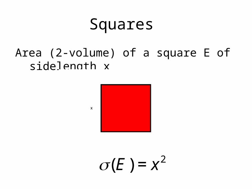
Squares

Area (2-volume) of a square E of sidelength x

€

€

σ(E) = x 2

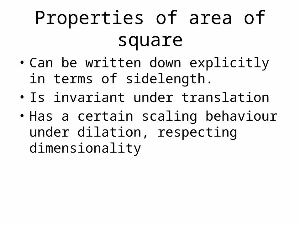
Properties of area of square

• Can be written down explicitly in terms of sidelength.

• Is invariant under translation• Has a certain scaling behaviour under dilation,

respecting dimensionality

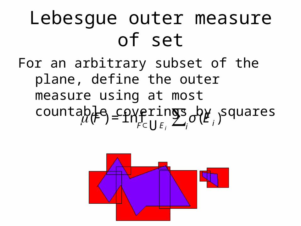
Lebesgue outer measure of set

For an arbitrary subset of the plane, define the outer measure using at most countable coverings by squares

€

μ(F) = infF⊂ E i

iU

σ (E i)i∑

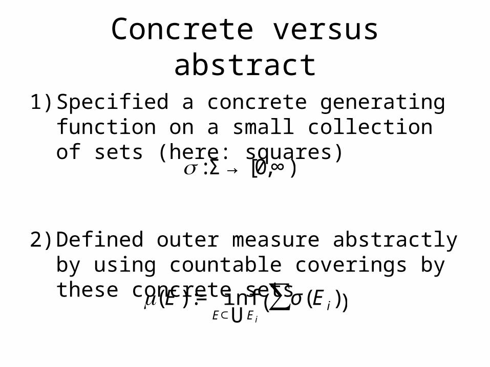
Concrete versus abstract

1) Specified a concrete generating function on a small collection of sets (here: squares)

2) Defined outer measure abstractly by using countable coverings by these concrete sets

€

σ : Σ →[0,∞)

€

μ(E) := infE⊂ E iU

σ (E i)∑( )

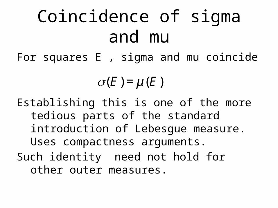
Coincidence of sigma and mu

For squares E , sigma and mu coincide

Establishing this is one of the more tedious parts of the standard introduction of Lebesgue measure. Uses compactness arguments.

Such identity need not hold for other outer measures.

€

σ(E) = μ(E)

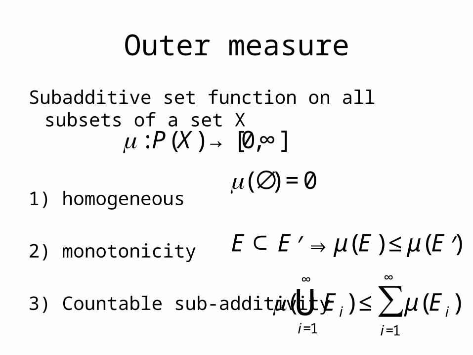
Outer measure

Subadditive set function on all subsets of a set X

1) homogeneous

2) monotonicity

3) Countable sub-additivity

€

μ : P(X) →[0,∞]

€

μ(∅ ) = 0

€

E ⊂ ′ E ⇒ μ(E) ≤ μ( ′ E )

€

μ( E i)i=1

∞

U ≤ μ(E i)i=1

∞

∑

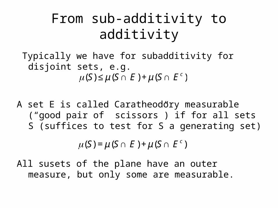
From sub-additivity to additivity

Typically we have for subadditivity for disjoint sets, e.g.

A set E is called Caratheodory measurable (“good pair of scissors”) if for all sets S (suffices to test for S a generating set)

All susets of the plane have an outer measure, but only some are measurable. €

μ(S) = μ(S ∩ E) + μ(S ∩ E c )

€

μ(S) ≤ μ(S ∩ E) + μ(S ∩ E c )

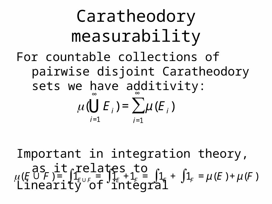
Caratheodory measurability

For countable collections of pairwise disjoint Caratheodory sets we have additivity:

Important in integration theory, as it relates toLinearity of integral

€

μ( E i) = μ(E i)i=1

∞

∑i=1

∞

U

€

μ(E ∪F) = 1E∪F = 1E +1F∫∫ = 1E∫ + 1F = μ(E) + μ(F)∫

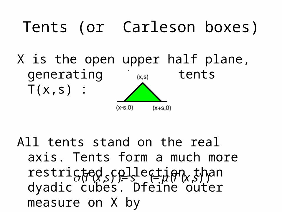
Tents (or Carleson boxes)

X is the open upper half plane, generating sets are tents T(x,s) :

All tents stand on the real axis. Tents form a much more restricted collection than dyadic cubes. Dfeine outer measure on X by

€

σ(T(x,s)) := s (= μ(T(x,s)))

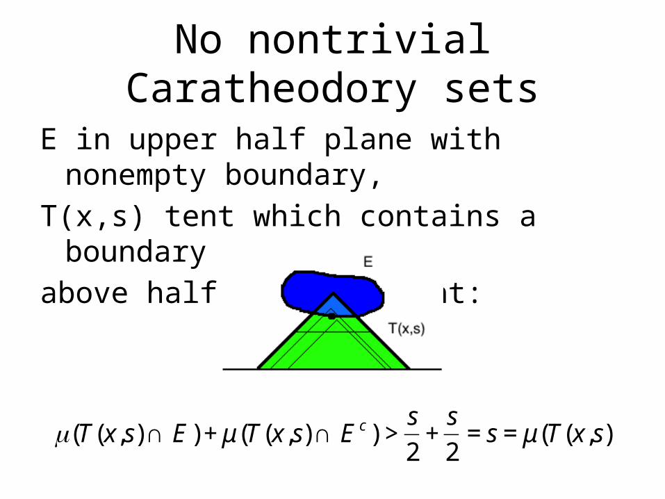
No nontrivial Caratheodory sets

E in upper half plane with nonempty boundary,T(x,s) tent which contains a boundary point of E above half of its height:

€

μ(T(x,s) ∩ E) + μ(T(x,s) ∩ E c ) >s

2+

s

2= s = μ(T(x,s))

Integration theory

Try to generalize measure to functions (which can be viewed as “weighted” sets.

Identifying measurable set E with the characteristic function

An integration theory for outer measures will not be linear. Theory of norms rather than integral.

€

μ(E) = 1E∫

Classical Choquet integral

If f is a function on outer measure space, may define

We will generalize this definition, following aConcrete-to-abstract principle as in the definition of outer measure.€

fp

p:= μ x :| f (x) |> λ{ }( )

0

∞

∫ λ pdλ /λ

Concrete average, size

Will play for norms of functions the same role as the assignment for the definition of outer measure. In case of Lebesgue measure for a given nonnegative function f and a dyadic cube Q

In caes of Lebesgue: The size contains enough information to reproduce f, it is a more efficient code than pointwise a.e information. It is redundant information, a countable collection of squares suffices.€

S( f )(Q) =1

| Q |f (x)dx

Q

∫€

σ(Q) = l(Q)n

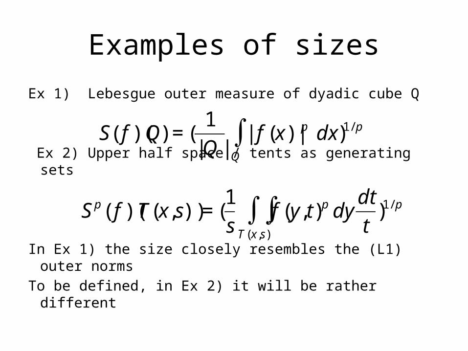
Examples of sizes

Ex 1) Lebesgue outer measure of dyadic cube Q

Ex 2) Upper half space / tents as generating sets

In Ex 1) the size closely resembles the (L1) outer normsTo be defined, in Ex 2) it will be rather different

€

S( f )(Q) = (1

| Q || f (x) |p dx

Q

∫ )1/ p

€

S p ( f )(T(x,s)) = (1

sf (y, t)p dy

dt

tT (x,s)

∫∫ )1/ p

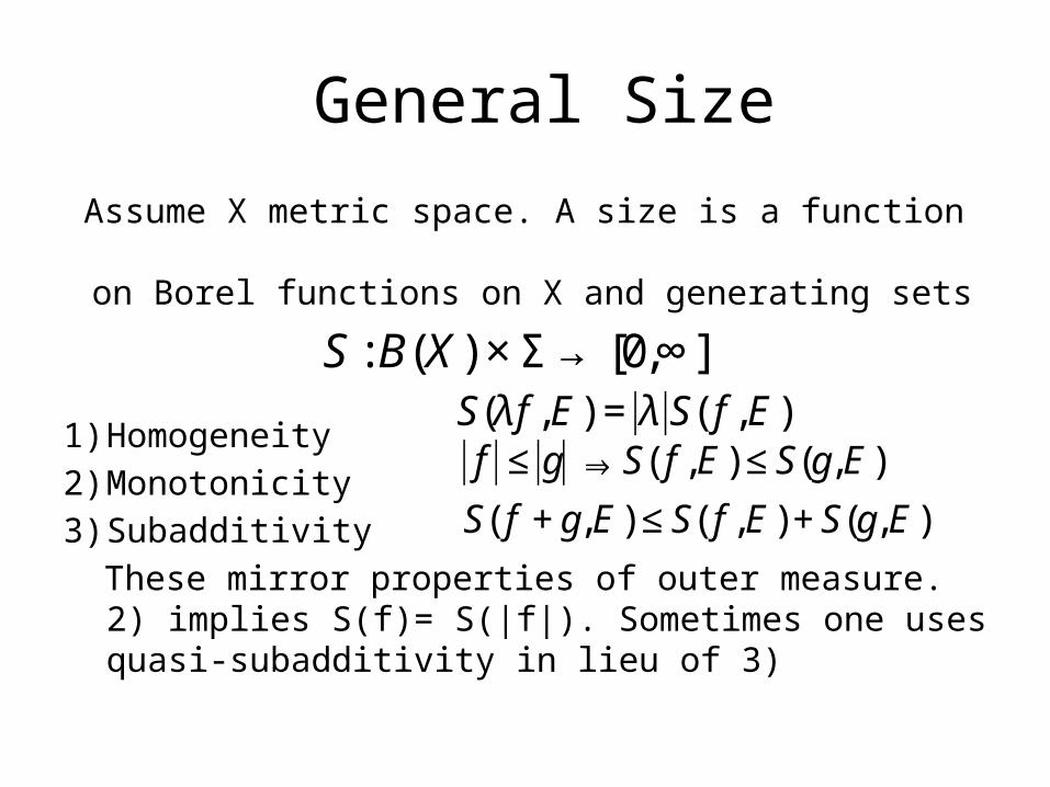
General Size

Assume X metric space. A size is a function on Borel functions on X and generating sets

1) Homogeneity2) Monotonicity3) Subadditivity These mirror properties of outer measure. 2) implies S(f)=

S(|f|). Sometimes one uses quasi-subadditivity in lieu of 3)

€

S : B(X) × Σ →[0,∞]

€

S(λ f ,E) = λ S( f ,E)

€

f ≤ g ⇒ S( f ,E) ≤ S(g,E)

€

S( f + g, E) ≤ S( f , E) + S(g, E)

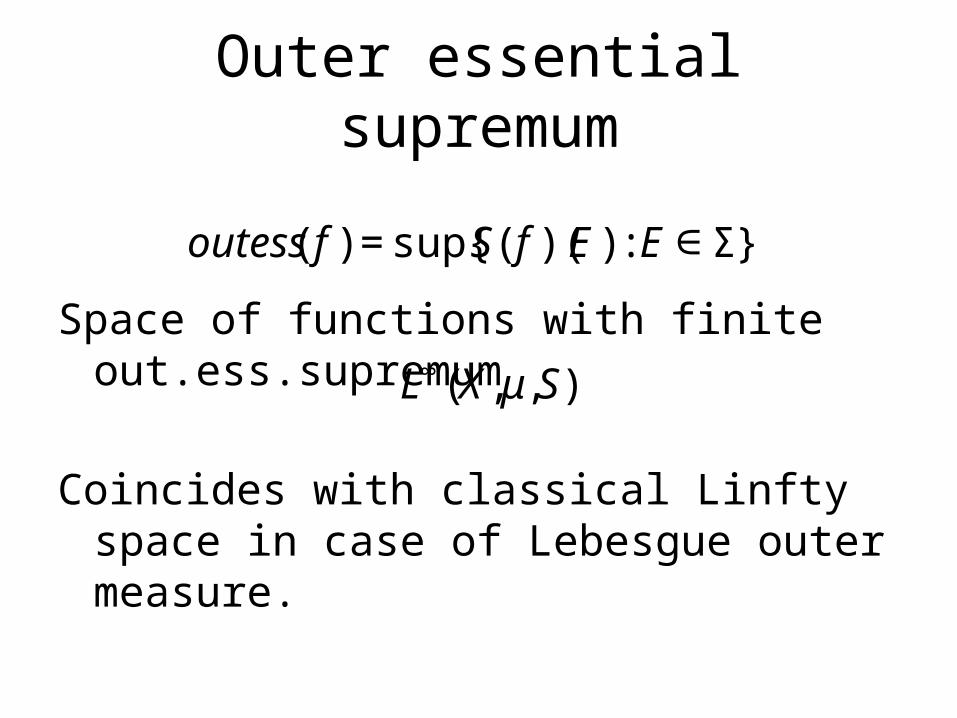
Outer essential supremum

Space of functions with finite out.ess.supremum

Coincides with classical Linfty space in case of Lebesgue outer measure.

€

outess( f ) = sup{S( f )(E) : E ∈Σ}

€

L∞(X,μ,S)

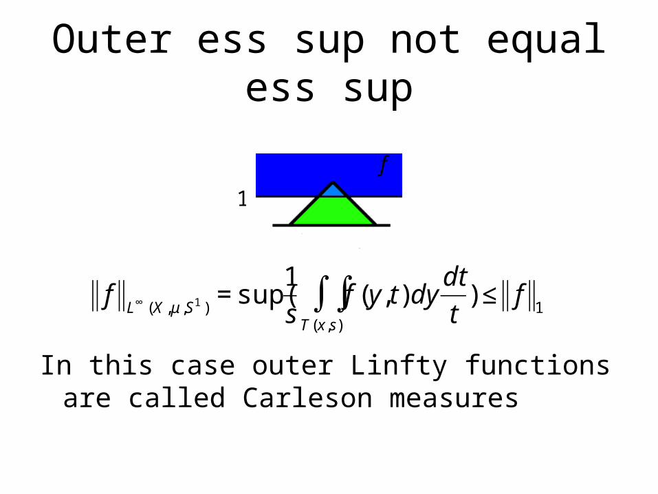
Outer ess sup not equal ess sup

In this case outer Linfty functions are called Carleson measures€

fL∞ (X ,μ ,S1 )

= sup(1

sf (y, t)dy

dt

tT (x,s)

∫∫ ) ≤ f1

€

1

€

f

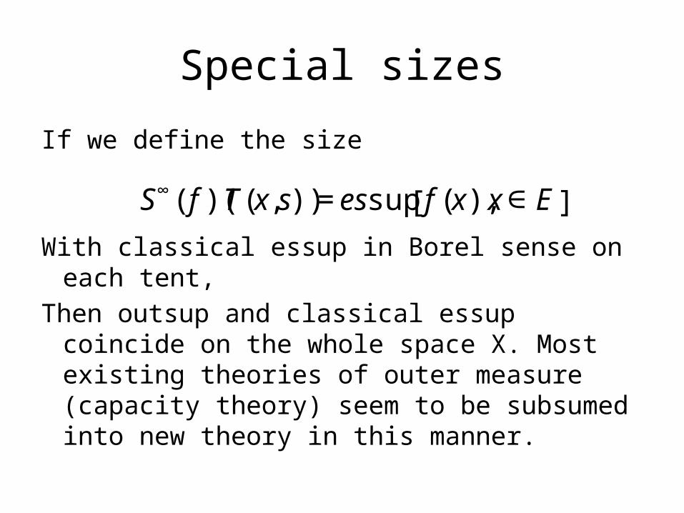
Special sizes

If we define the size

With classical essup in Borel sense on each tent,Then outsup and classical essup coincide on the

whole space X. Most existing theories of outer measure (capacity theory) seem to be subsumed into new theory in this manner.

€

S∞( f )(T(x,s)) = essup f (x), x ∈E[ ]

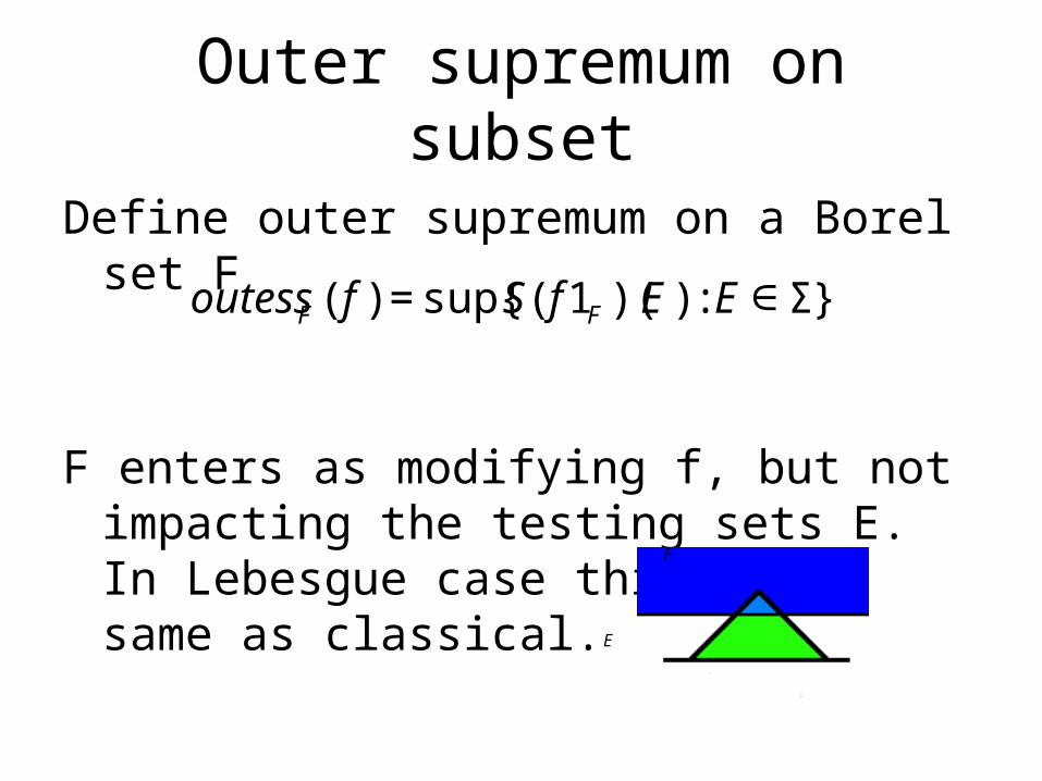
Outer supremum on subset

Define outer supremum on a Borel set F

F enters as modifying f, but not impacting the testing sets E. In Lebesgue case this gives same as classical.

€

outessF ( f ) = sup{S( f 1F )(E) : E ∈Σ}

€

F

€

E

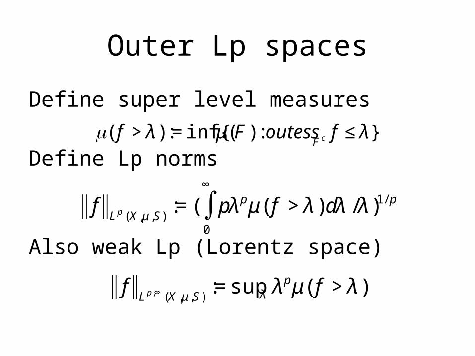
Outer Lp spaces

Define super level measures

Define Lp norms

Also weak Lp (Lorentz space) €

μ( f > λ ) := inf{μ(F) : outessF c f ≤ λ}

€

fLp (X ,μ ,S )

:= ( pλ p

0

∞

∫ μ( f > λ )dλ /λ )1/ p

€

fLp ,∞ (X ,μ ,S )

:= supλ λ pμ( f > λ )

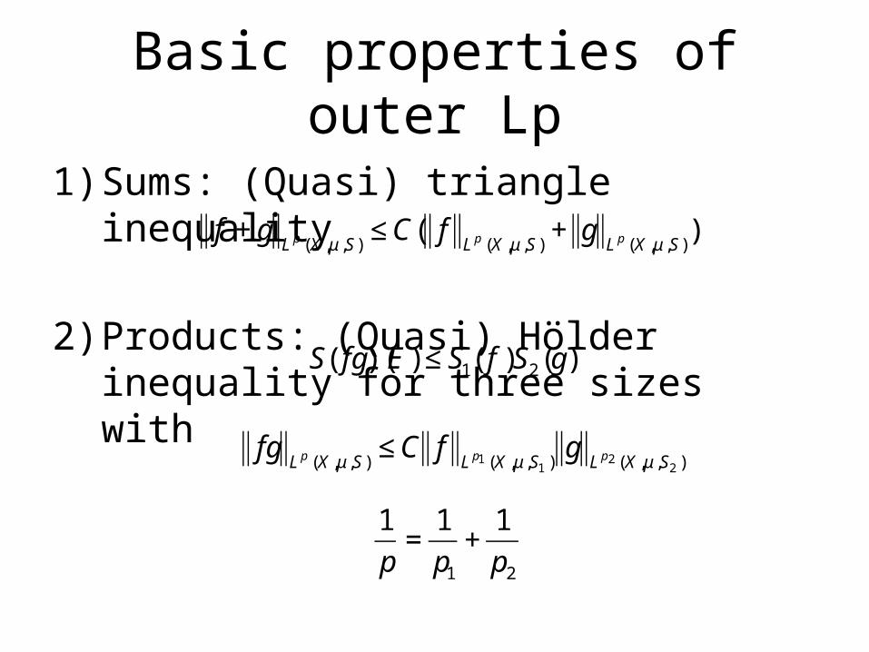
Basic properties of outer Lp

1) Sums: (Quasi) triangle inequality

2) Products: (Quasi) Hölder inequality for three sizes with

€

f + gLp (X ,μ ,S )

≤ C( fLp (X ,μ ,S )

+ gLp (X ,μ ,S )

)

€

S( fg)(E) ≤ S1( f )S2(g)

€

fgLp (X ,μ ,S )

≤ C fLp1 (X ,μ ,S1 )

gLp2 (X ,μ ,S2 )

€

1

p=

1

p1

+1

p2

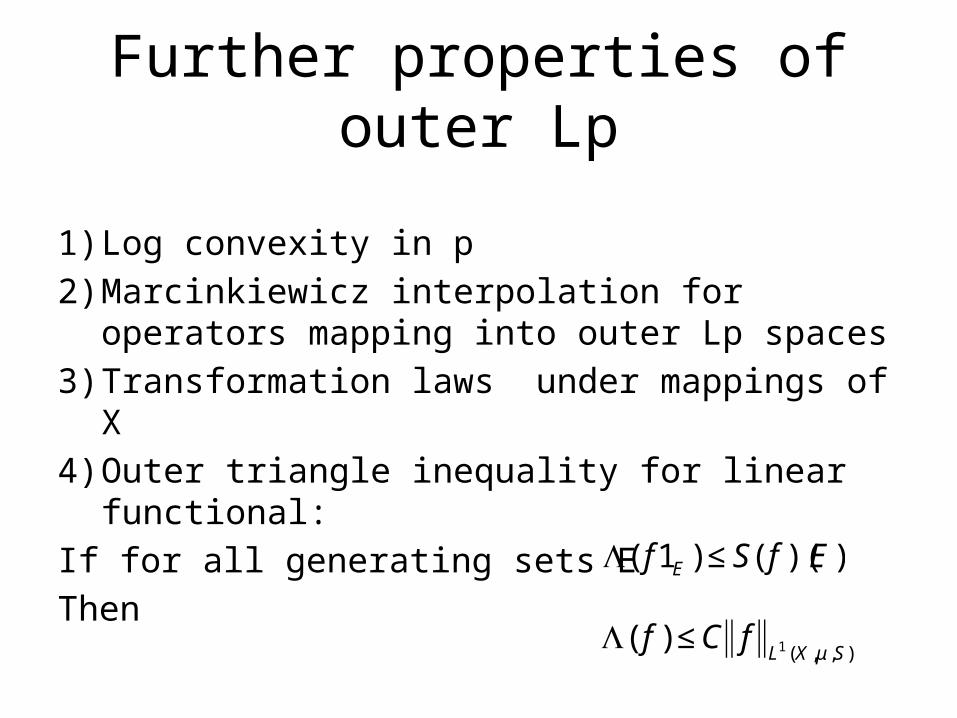
Further properties of outer Lp

1) Log convexity in p2) Marcinkiewicz interpolation for operators

mapping into outer Lp spaces3) Transformation laws under mappings of X4) Outer triangle inequality for linear functional:If for all generating sets EThen

€

Λ( f ) ≤ C fL1 (X ,μ ,S )

€

Λ( f 1E ) ≤ S( f )(E)

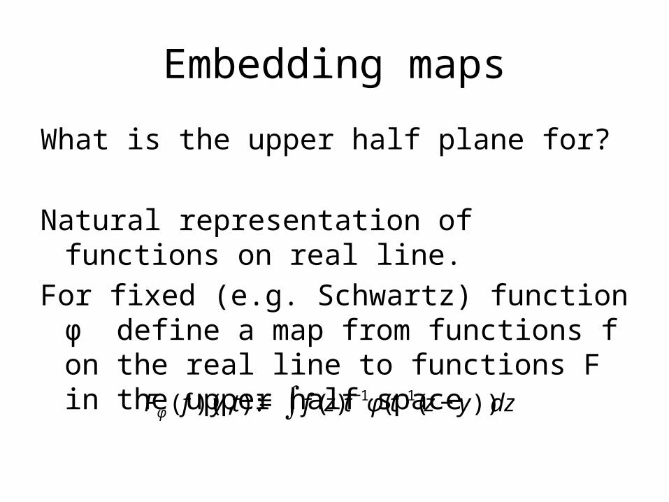
Embedding maps

What is the upper half plane for?

Natural representation of functions on real line.For fixed (e.g. Schwartz) function ϕ define a

map from functions f on the real line to functions F in the upper half space

€

Fφ ( f )(y, t) := f (z)t−1φ(t−1(z − y))dz∫

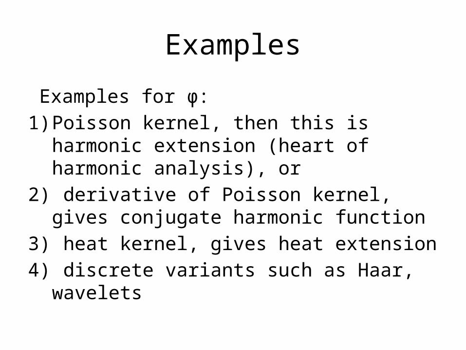
Examples

Examples for ϕ: 1) Poisson kernel, then this is harmonic

extension (heart of harmonic analysis), or 2) derivative of Poisson kernel, gives conjugate

harmonic function 3) heat kernel, gives heat extension 4) discrete variants such as Haar, wavelets

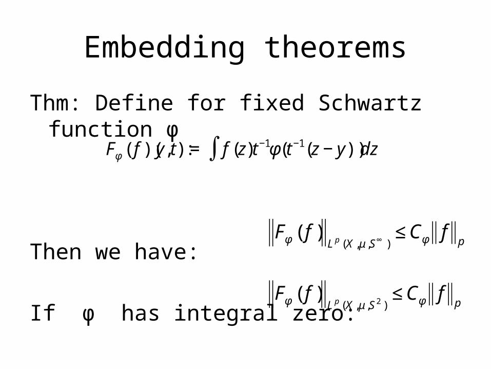
Embedding theorems

Thm: Define for fixed Schwartz function ϕ

Then we have:

If φ has integral zero:

€

Fφ ( f )(y, t) := f (z)t−1φ(t−1(z − y))dz∫

€

Fφ ( f )Lp (X ,μ ,S ∞ )

≤ Cφ fp

€

Fφ ( f )Lp (X ,μ ,S 2 )

≤ Cφ fp