Embed Size (px)
Citation preview

An-Najah National University
Faculty of Graduate Studies
An Iterative Method for Optimally
Sizing Solar Inverter in Grid
Connected System:
A Case Study of Palestine
By
Ali Ahmad Ali Mohammad
Supervisor
Dr. Tamer khatib
This Thesis is Submitted in Partial Fulfillment of the Requirements for
the Degree of Master of Engineering in Clean Energy and
Conservation Strategy, Faculty of Graduate Studies, An-Najah
National University, Nablus, Palestine
2016
II
An Iterative Method for Optimally Sizing Solar
Inverter in Grid Connected System: A Case Study of
Palestine
By
Ali Ahmad Ali Mohammad
This thesis was defended successfully on 15 /12/2016 and approved by:
Defense committee Members Signature
Dr. Tamer khatib /Supervisor ………………..
Dr. Maher Maghalseh /External Examiner …..……………
Dr. Aysar yasin /Internal Examiner …..……………

III
Dedication
To my parents
To my wife
To my son Anas
To my daughters Sara, Danya and Jana
To all of them,
I dedicate this work

IV
Acknowledgments
It is an honor for me to have the opportunity to thank all people who helped
me to conduct this study. All appreciations go to my supervisor, Dr. Tamer
Khatib for his exceptional guidance and insightful comments and
observations throughout the duration of this project.My thanks and
appreciations go to the staff of Clean Energy and Conservation Strategy
Engineering Master Program in An-Najah National University, especially
Prof. Dr. Marwan Mahmoud for his assistance.
.
V
الإقرار
أنا الموقع أدناه مقدم الرسالة التي تحمل عنوان
An Iterative Method for Optimally Sizing Solar
Inverter in Grid Connected System: A Case Study of
Palestine
إليه لإشارةتمت ا ما باستثناء الخاص، جهدي نتاج هو إنما الرسالة هذه عليه اشتملت ما بأن أقر
علمي لقب وأدرجة أي لنيل قبل من يقدم لم منها جزء أي أو كاملة، الرسالة هذه ورد، وأن حيثما
.أخرى بحثية أو مؤسسة تعليمية أي لدى بحثي أو
Declaration
The work provided in this thesis, unless otherwise referenced, is the
researcher's own work, and has not been submitted elsewhere for any other
degree or qualification.
Student's name: :اسم الطالب
Signature: التوقيع:
Date: : التاريخ
VI
Table of Contents Dedication ................................................................................................... III
Acknowledgments ....................................................................................... IV
Declaration ................................................................................................... V
Table of Contents ........................................................................................ VI
List of Tables ............................................................................................. VII
List of Figures .......................................................................................... VIII
Abstract ....................................................................................................... IX
Chapter One ................................................................................................... 1
Introduction ................................................................................................... 1
1.1 Background .......................................................................................... 1
1.3 Problem statement : .............................................................................. 3
1.4 Objectives: ............................................................................................ 4
1.5 Methodology ........................................................................................ 4
Chapter Two .................................................................................................. 6
Literature review ........................................................................................... 6
Chapter Three .............................................................................................. 17
3.1 Introduction …….…………………………………………………….18
3.2 Frequency distribution analysis for adapted solar radiation data ......... 17
3.3 Proposed numerical iterative method for calculating the optimum size
of inverter. ................................................................................................... 19
3.4 Validation of thesis's propos………………………………………….27
Chapter Four ................................................................................................ 32
Results and discussion ................................................................................. 32
4.1 Introduction …….…………………………………………………….18
Case1: the capacity of inverter matches the PV array capacity ............... 35
Case2: the inverter is optimally installed according to the sizing ratio ... 37
Chapter Five ................................................................................................ 38
5.1 Conclusion .......................................................................................... 39
5.2 Future work: ....................................................................................... 40
References ................................................................................................... 41
Appendix …………………………………………………………………39

VII
List of Tables Table (3. 1) : Inverter models coefficients .................................................. 24
Table (4. 1) : Optimum inverter sizes (Rs) for different locations. ............ 34
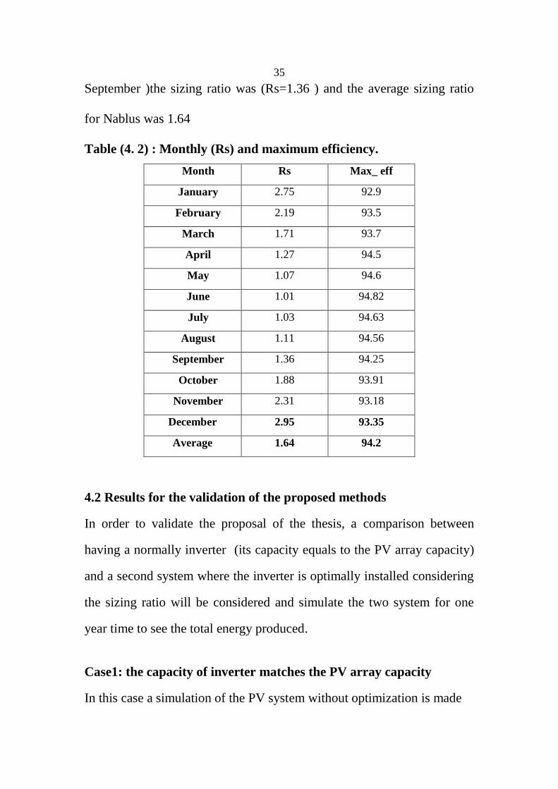
Table (4. 2) : Monthly (Rs) and maximum efficiency. ............................... 35
Table (4. 3) : Comparison between tow cases. ........................................... 38
VIII
List of Figures
Figure (3. 1): most frequent solar radiation . .............................................. 18
Figure (4. 1): searching for the optimum inverter size . ............................. 33
Figure (4. 2): the capacity of inverter equals the PV array capacity. ......... 28
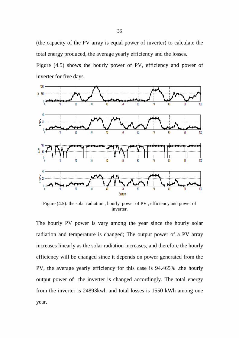
Figure (4. 3): the hourly power of PV , efficiency and power of inverter for
five days . ............................................................................... 36
Figure (4. 4): the inverter is optimally installed according to the sizing ratio
(Pinv is 60% of Ppv). ............................................................. 30
Figure (4. 5): the hourly power of PV , efficiency and power of inverter for
five days . ............................................................................... 37
IX
An Inverter Method for Optimally Sizing Solar Inverter in Grid
Connected System: A Case Study of Palestine
By
Ali ahmad ali mohamad
Supervisor
Dr. Tamer khatib
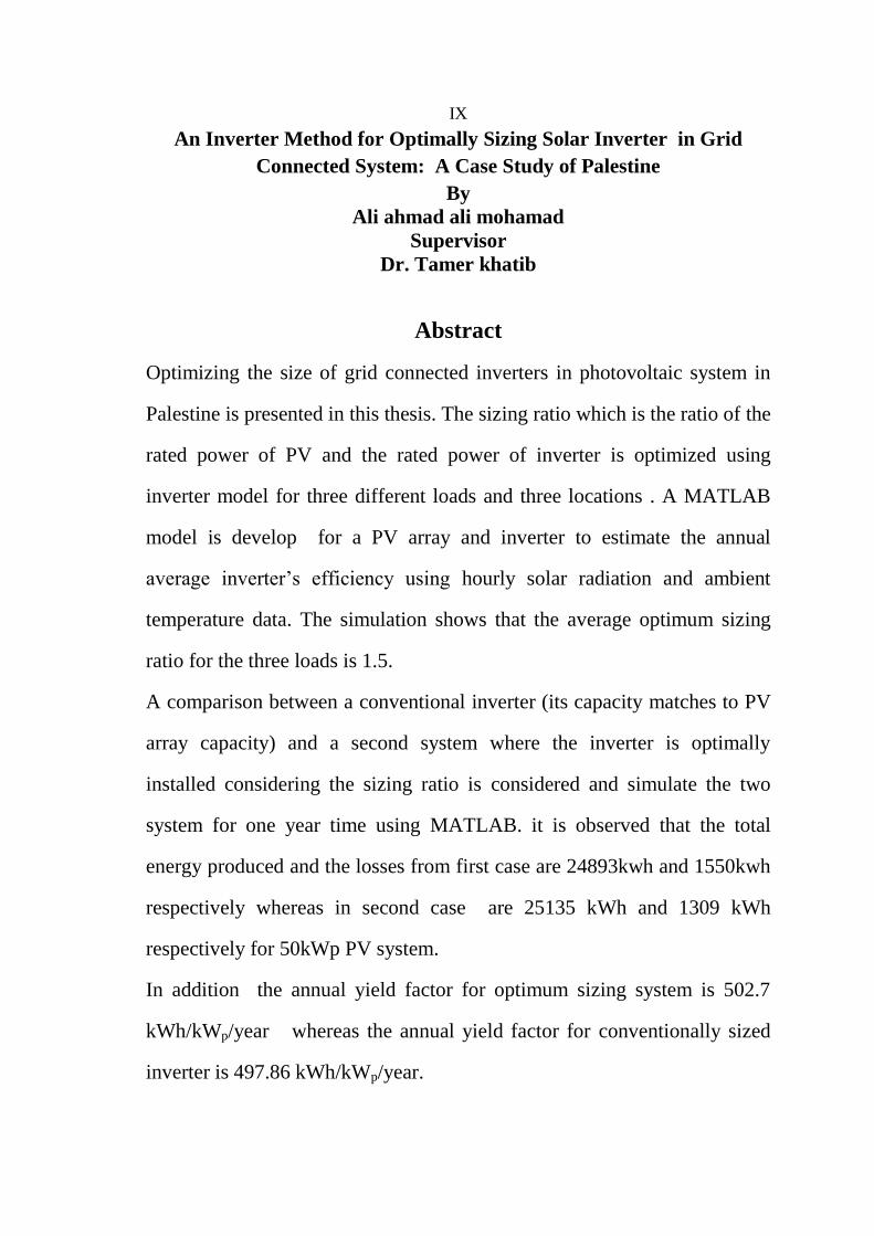
Abstract
Optimizing the size of grid connected inverters in photovoltaic system in
Palestine is presented in this thesis. The sizing ratio which is the ratio of the
rated power of PV and the rated power of inverter is optimized using
inverter model for three different loads and three locations . A MATLAB
model is develop for a PV array and inverter to estimate the annual
average inverter’s efficiency using hourly solar radiation and ambient
temperature data. The simulation shows that the average optimum sizing
ratio for the three loads is 1.5.
A comparison between a conventional inverter (its capacity matches to PV
array capacity) and a second system where the inverter is optimally
installed considering the sizing ratio is considered and simulate the two
system for one year time using MATLAB. it is observed that the total
energy produced and the losses from first case are 24893kwh and 1550kwh
respectively whereas in second case are 25135 kWh and 1309 kWh
respectively for 50kWp PV system.
In addition the annual yield factor for optimum sizing system is 502.7
kWh/kWp/year whereas the annual yield factor for conventionally sized
inverter is 497.86 kWh/kWp/year.
1
Chapter One
Introduction
1.1 Background
The increasing use of renewable energy is attributed not only to global
warming but also the ease of the free resource available from nature.
Since fossil fuel is the most commonly used source of energy to meet the
energy demands of the world for a long time, there has been a fast
reduction of fossil fuel deposits in the world and consequently in the near
future a big shortage of energy is expected to happen if the trend
continues this way. Therefore, there is a need to find better sustainable
energy solutions to preserve the earth for the future generations in the
world [Santra,2012].
Solar energy is free energy from the sun and it is renewable, unlimited
and friendly to environment. Photovoltaic (PV) energy generation is one
of the applications of direct solar energy utilization. These systems have
been spread lately due to the increase in energy consumption and the
resulting environmental pollution. PV systems can be classified into three
systems, standalone, grid connected and hybrid PV systems. Grid
connected PV systems are directly connected to the grid and inject their
production directly to the grid. These systems are usually called
distribution generation units. A distribution generation unit is an electric

2
power generator which produces electricity at a location close to the loads
and can be tied to electrical utility. Thus it can be used to generate a part
of electricity demanded by consumers to reduce electricity that purchased
from utility grid especially at peak demands and at emergency situation.
Distribution generation has many benefits such as it has less initial cost
than conventional sources, does not need large area as in large power
plant, reduce loading on transmission lines, produces less pollutant
emissions, increases power system’s reliability since it can act as backup
power source .
However, the obstacle of using grid connected PV system is the high
initial cost and low overall efficiency. Moreover, there are some
challenges to such systems in terms of power systems such as the
negative impact on the electrical network in terms of power quality,
system’s voltage levels due to the injected power and system protection.
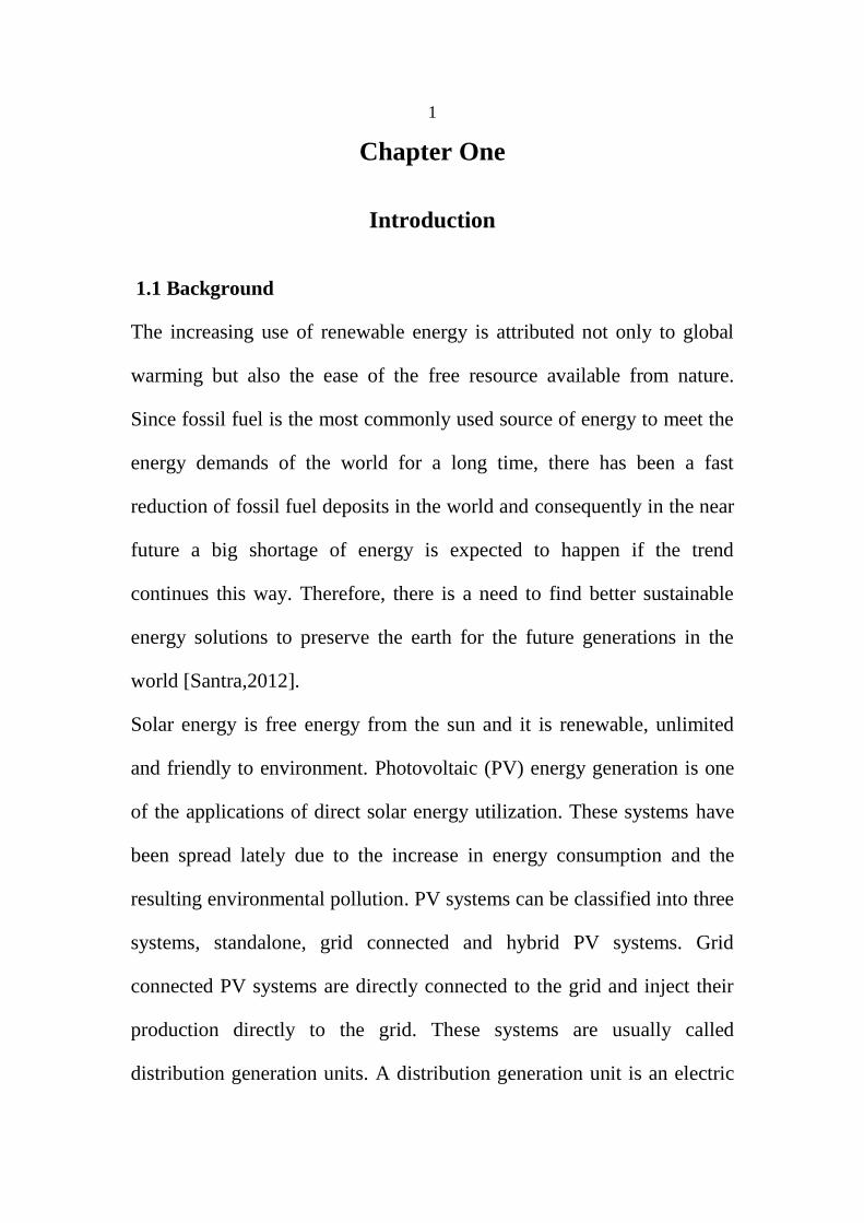
A typical grid connected PV system is shown in figure (1.1). In this
system the photovoltaic are designed to be connected to the utility grid
through a grid tied inverter (GTI) which is used to convert the direct
current that comes from the PV array to an alternating current so as to
ensure that the shape of the output wave is matching the voltage and
frequency of the electrical network (pure sine wave, THD<3%). Many
factors should be considered for GTI such as the input voltage that must
be matched with the nominal voltage of the PV array. Moreover, the
3
nominal power of inverter should also be matched with the DC power of
the array as well as GTI conversion efficiency.
GTIs are usually sized according to the rated power of the PV array,
rather than the load requirements. Also GTIs usually include maximum
power point tracking to ensure maximum power injection [Yasin,2008].
Figure (1.1): Grid-connected PV power system
1.3 Problem statement :
Since the solar resource is not always stable, the output power from PV
panels is also not always stable. To maximize the output power from
photovoltaic array, many previous researches were carried out in the field
of PV systems so as to have the PV panels of the system optimally
matched to the inverter's rated power [Khatib,2012]. At low solar
radiation levels, PV array generates less power than its rated power and
accordingly the inverter is operated with lower inverter efficiency
[Keller,1995.Coppye, 1995]. Thus, finding the optimal size of a grid
connected inverter acts an important role in increasing total energy
produced by the PV system. To optimize the inverter size, local solar
PV Array Inverter
Main
Distribution
Panel
Grid
Local Loads
4
radiation, ambient temperature and inverter efficiency curve are needed
[Macagnan,1992. Jantsch, 1992]. Thus, it must be taken in to account
that the optimization of the inverter’s size of in PV system is a location
dependent process. In the meanwhile, such an optimization was not
conducted in Palestine considering Palestinian climate.
1.4 Objectives:
1- To optimally size a grid connected solar inverter using a numerical
algorithm.
2- To conduct a comparison between the proposal of this thesis and a
PV system with conventionally sized inverter.
1.5 Methodology
The research work in this thesis is divided into work packages and tasks
as described below:
WP.1 Literature review
T.1 A review of current optimization methods for calculating the
optimum size of grid inverter in PV System.
WP.2 Data collection and analysis
T.1 Collection of solar radiation and ambient temperature data for
Palestine.
T.2 Frequency distribution analysis of these data.
WP.3 Modeling of grid connected PV system.
T.1 Modeling of PV array output power

5
T.2 Modeling of grid connected inverter efficiency
WP.4 Optimal sizing of the solar inverter
T.1 optimal sizing of PV inverter considering solar radiation and ambient
temperature data as well inverter’s efficiency model for three inverters
types using MATLAB
T.2 Conduct between the cases of having a normally installed inverter
and an optimally installed inverter using MATLAB to validate the
proposal of this thesis.
WP.5 Thesis writing
T.1 Thesis writing
T.2 Research paper writing and submission
6
Chapter Two
Literature review
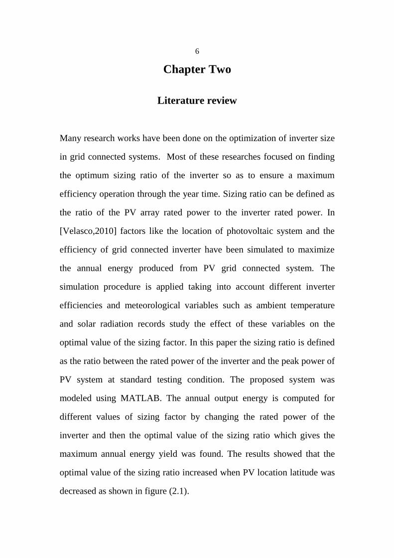
Many research works have been done on the optimization of inverter size
in grid connected systems. Most of these researches focused on finding
the optimum sizing ratio of the inverter so as to ensure a maximum
efficiency operation through the year time. Sizing ratio can be defined as
the ratio of the PV array rated power to the inverter rated power. In
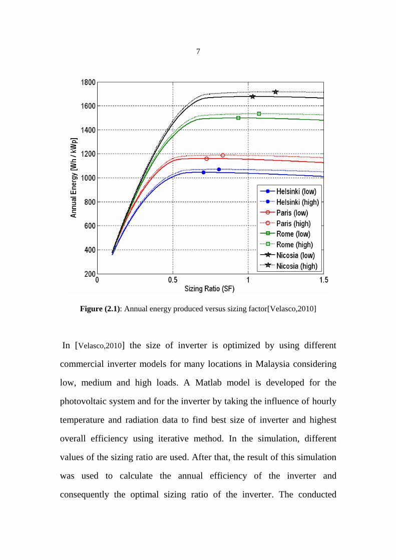
[Velasco,2010] factors like the location of photovoltaic system and the
efficiency of grid connected inverter have been simulated to maximize
the annual energy produced from PV grid connected system. The
simulation procedure is applied taking into account different inverter
efficiencies and meteorological variables such as ambient temperature
and solar radiation records study the effect of these variables on the
optimal value of the sizing factor. In this paper the sizing ratio is defined
as the ratio between the rated power of the inverter and the peak power of
PV system at standard testing condition. The proposed system was
modeled using MATLAB. The annual output energy is computed for
different values of sizing factor by changing the rated power of the
inverter and then the optimal value of the sizing ratio which gives the
maximum annual energy yield was found. The results showed that the
optimal value of the sizing ratio increased when PV location latitude was
decreased as shown in figure (2.1).
7
Figure (2.1): Annual energy produced versus sizing factor[Velasco,2010]
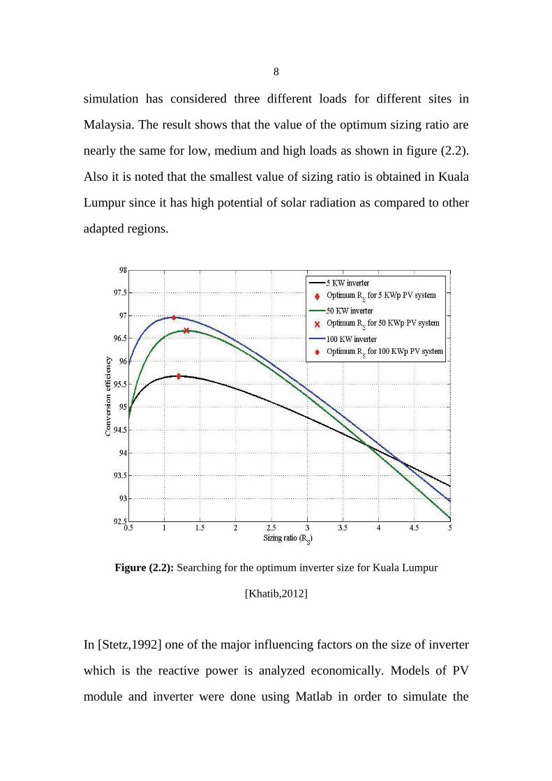
In [Velasco,2010] the size of inverter is optimized by using different
commercial inverter models for many locations in Malaysia considering
low, medium and high loads. A Matlab model is developed for the
photovoltaic system and for the inverter by taking the influence of hourly
temperature and radiation data to find best size of inverter and highest
overall efficiency using iterative method. In the simulation, different
values of the sizing ratio are used. After that, the result of this simulation
was used to calculate the annual efficiency of the inverter and
consequently the optimal sizing ratio of the inverter. The conducted
8
simulation has considered three different loads for different sites in
Malaysia. The result shows that the value of the optimum sizing ratio are
nearly the same for low, medium and high loads as shown in figure (2.2).
Also it is noted that the smallest value of sizing ratio is obtained in Kuala
Lumpur since it has high potential of solar radiation as compared to other
adapted regions.
Figure (2.2): Searching for the optimum inverter size for Kuala Lumpur
[Khatib,2012]
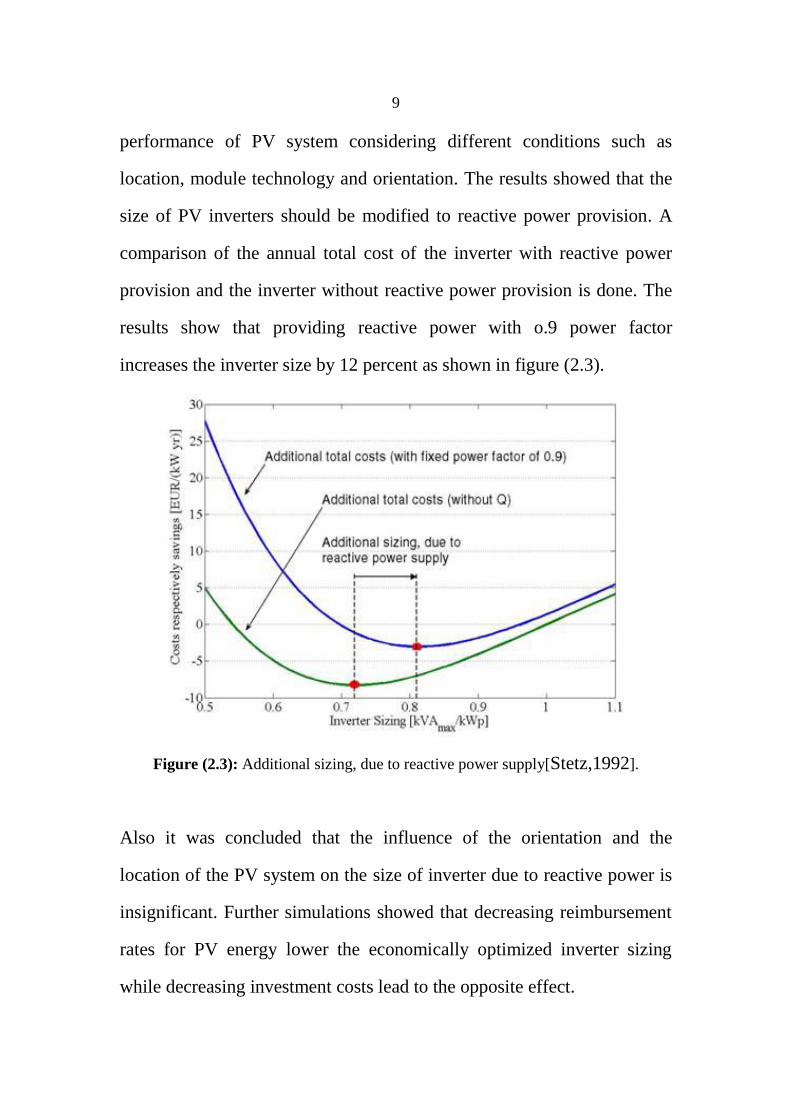
In [Stetz,1992] one of the major influencing factors on the size of inverter
which is the reactive power is analyzed economically. Models of PV
module and inverter were done using Matlab in order to simulate the
9
performance of PV system considering different conditions such as
location, module technology and orientation. The results showed that the
size of PV inverters should be modified to reactive power provision. A
comparison of the annual total cost of the inverter with reactive power
provision and the inverter without reactive power provision is done. The
results show that providing reactive power with o.9 power factor
increases the inverter size by 12 percent as shown in figure (2.3).
Figure (2.3): Additional sizing, due to reactive power supply[Stetz,1992].
Also it was concluded that the influence of the orientation and the
location of the PV system on the size of inverter due to reactive power is
insignificant. Further simulations showed that decreasing reimbursement
rates for PV energy lower the economically optimized inverter sizing
while decreasing investment costs lead to the opposite effect.
10
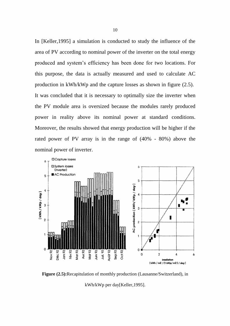
In [Keller,1995] a simulation is conducted to study the influence of the
area of PV according to nominal power of the inverter on the total energy
produced and system’s efficiency has been done for two locations. For
this purpose, the data is actually measured and used to calculate AC
production in kWh/kWp and the capture losses as shown in figure (2.5).
It was concluded that it is necessary to optimally size the inverter when
the PV module area is oversized because the modules rarely produced
power in reality above its nominal power at standard conditions.
Moreover, the results showed that energy production will be higher if the
rated power of PV array is in the range of (40% - 80%) above the
nominal power of inverter.
Figure (2.5):Recapitulation of monthly production (Lausanne/Switzerland), in
kWh/kWp per day[Keller,1995].
11
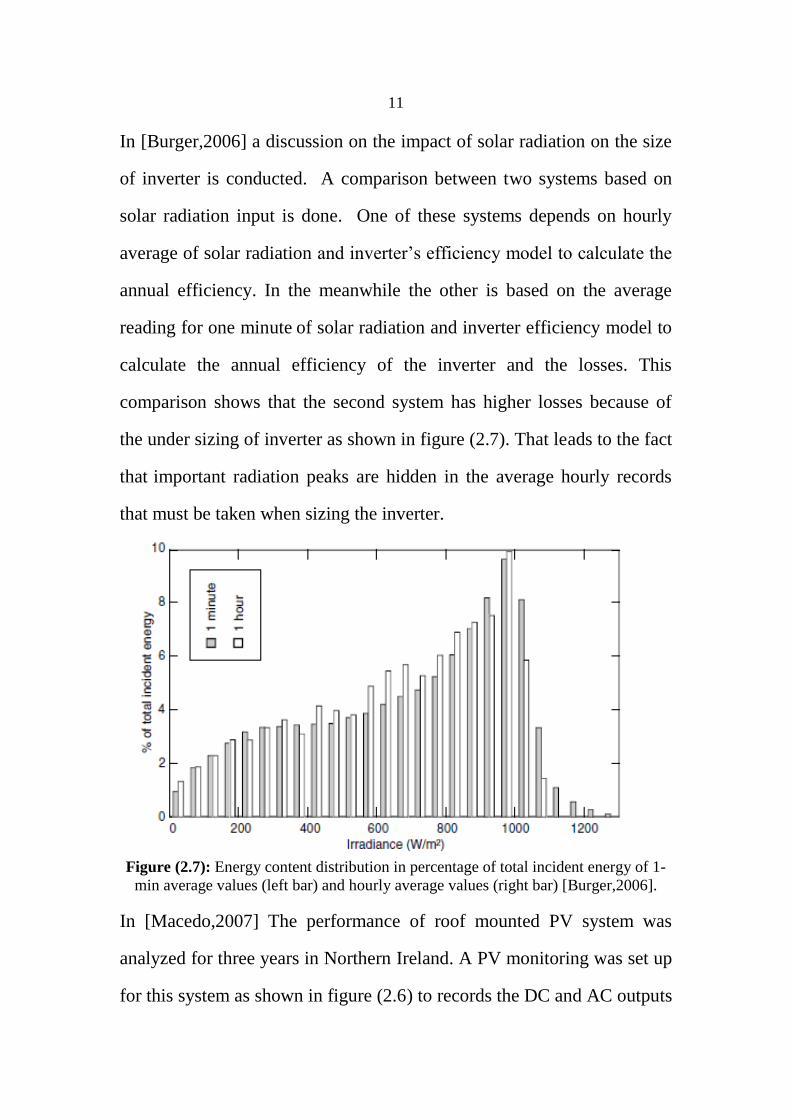
In [Burger,2006] a discussion on the impact of solar radiation on the size
of inverter is conducted. A comparison between two systems based on
solar radiation input is done. One of these systems depends on hourly
average of solar radiation and inverter’s efficiency model to calculate the
annual efficiency. In the meanwhile the other is based on the average
reading for one minute of solar radiation and inverter efficiency model to
calculate the annual efficiency of the inverter and the losses. This
comparison shows that the second system has higher losses because of
the under sizing of inverter as shown in figure (2.7). That leads to the fact
that important radiation peaks are hidden in the average hourly records
that must be taken when sizing the inverter.
Figure (2.7): Energy content distribution in percentage of total incident energy of 1-
min average values (left bar) and hourly average values (right bar) [Burger,2006].
In [Macedo,2007] The performance of roof mounted PV system was
analyzed for three years in Northern Ireland. A PV monitoring was set up
for this system as shown in figure (2.6) to records the DC and AC outputs
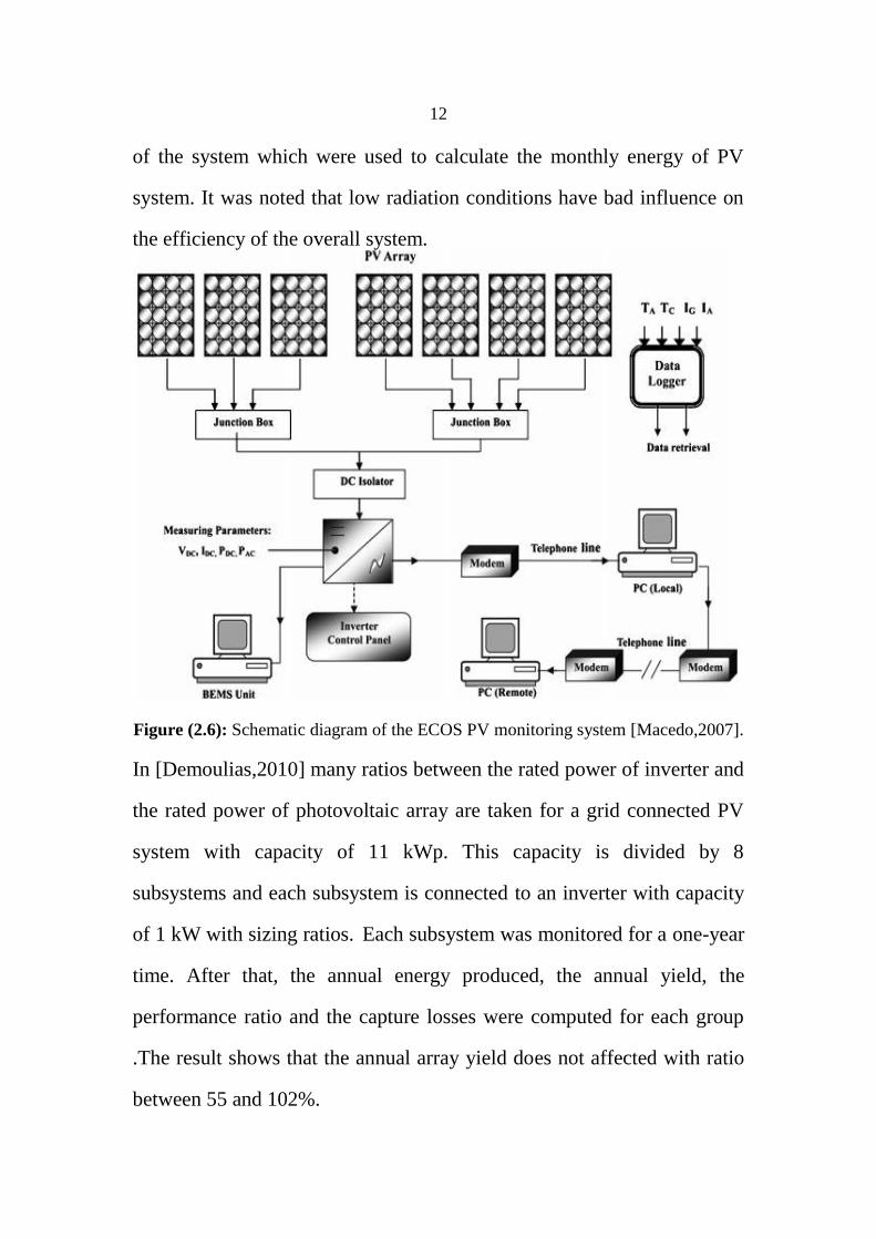
12
of the system which were used to calculate the monthly energy of PV
system. It was noted that low radiation conditions have bad influence on
the efficiency of the overall system.
Figure (2.6): Schematic diagram of the ECOS PV monitoring system [Macedo,2007].
In [Demoulias,2010] many ratios between the rated power of inverter and
the rated power of photovoltaic array are taken for a grid connected PV
system with capacity of 11 kWp. This capacity is divided by 8
subsystems and each subsystem is connected to an inverter with capacity
of 1 kW with sizing ratios. Each subsystem was monitored for a one-year
time. After that, the annual energy produced, the annual yield, the
performance ratio and the capture losses were computed for each group
.The result shows that the annual array yield does not affected with ratio
between 55 and 102%.
13
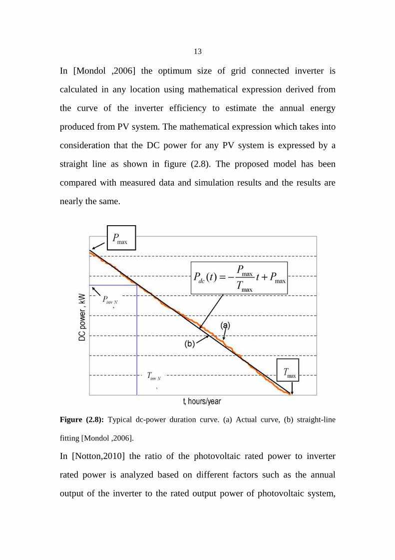
In [Mondol ,2006] the optimum size of grid connected inverter is
calculated in any location using mathematical expression derived from
the curve of the inverter efficiency to estimate the annual energy
produced from PV system. The mathematical expression which takes into
consideration that the DC power for any PV system is expressed by a
straight line as shown in figure (2.8). The proposed model has been
compared with measured data and simulation results and the results are
nearly the same.
Figure (2.8): Typical dc-power duration curve. (a) Actual curve, (b) straight-line
fitting [Mondol ,2006].
In [Notton,2010] the ratio of the photovoltaic rated power to inverter
rated power is analyzed based on different factors such as the annual
output of the inverter to the rated output power of photovoltaic system,
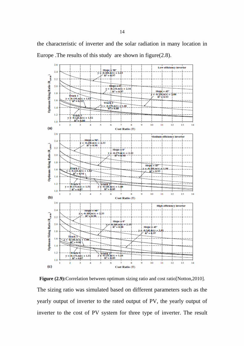
14
the characteristic of inverter and the solar radiation in many location in
Europe .The results of this study are shown in figure(2.8).
Figure (2.9):Correlation between optimum sizing ratio and cost ratio[Notton,2010].
The sizing ratio was simulated based on different parameters such as the
yearly output of inverter to the rated output of PV, the yearly output of
inverter to the cost of PV system for three type of inverter. The result
15
show that if the rated power of PV array is higher than the rated power of
inverter, the optimum performance is achieved when the cost of inverter
is increased in relation to the cost of PV. Also it was concluded that the
influence of sizing ratio on the performance of PV system is important for
inverter having low efficiency rather inverter having high efficiency.
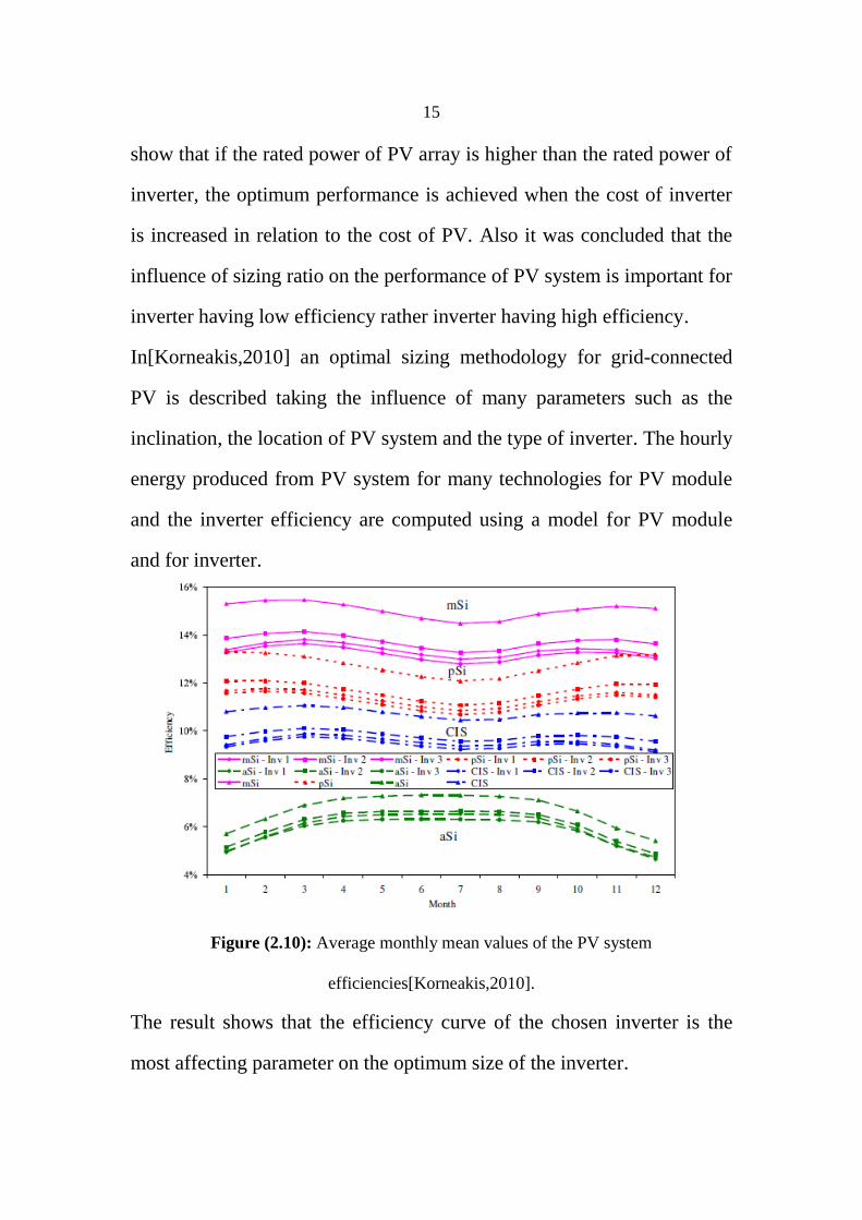
In[Korneakis,2010] an optimal sizing methodology for grid-connected
PV is described taking the influence of many parameters such as the
inclination, the location of PV system and the type of inverter. The hourly
energy produced from PV system for many technologies for PV module
and the inverter efficiency are computed using a model for PV module
and for inverter.
Figure (2.10): Average monthly mean values of the PV system
efficiencies[Korneakis,2010].
The result shows that the efficiency curve of the chosen inverter is the
most affecting parameter on the optimum size of the inverter.
16
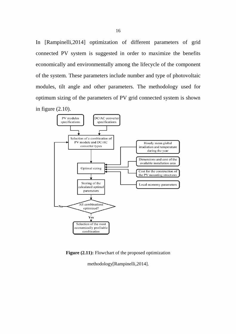
In [Rampinelli,2014] optimization of different parameters of grid
connected PV system is suggested in order to maximize the benefits
economically and environmentally among the lifecycle of the component
of the system. These parameters include number and type of photovoltaic
modules, tilt angle and other parameters. The methodology used for
optimum sizing of the parameters of PV grid connected system is shown
in figure (2.10).
Figure (2.11): Flowchart of the proposed optimization
methodology[Rampinelli,2014].
17
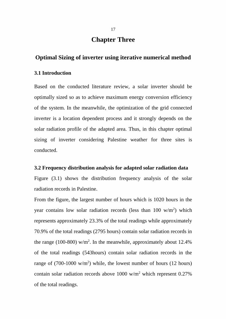
Chapter Three
Optimal Sizing of inverter using iterative numerical method
3.1 Introduction
Based on the conducted literature review, a solar inverter should be
optimally sized so as to achieve maximum energy conversion efficiency
of the system. In the meanwhile, the optimization of the grid connected
inverter is a location dependent process and it strongly depends on the
solar radiation profile of the adapted area. Thus, in this chapter optimal
sizing of inverter considering Palestine weather for three sites is
conducted.
3.2 Frequency distribution analysis for adapted solar radiation data
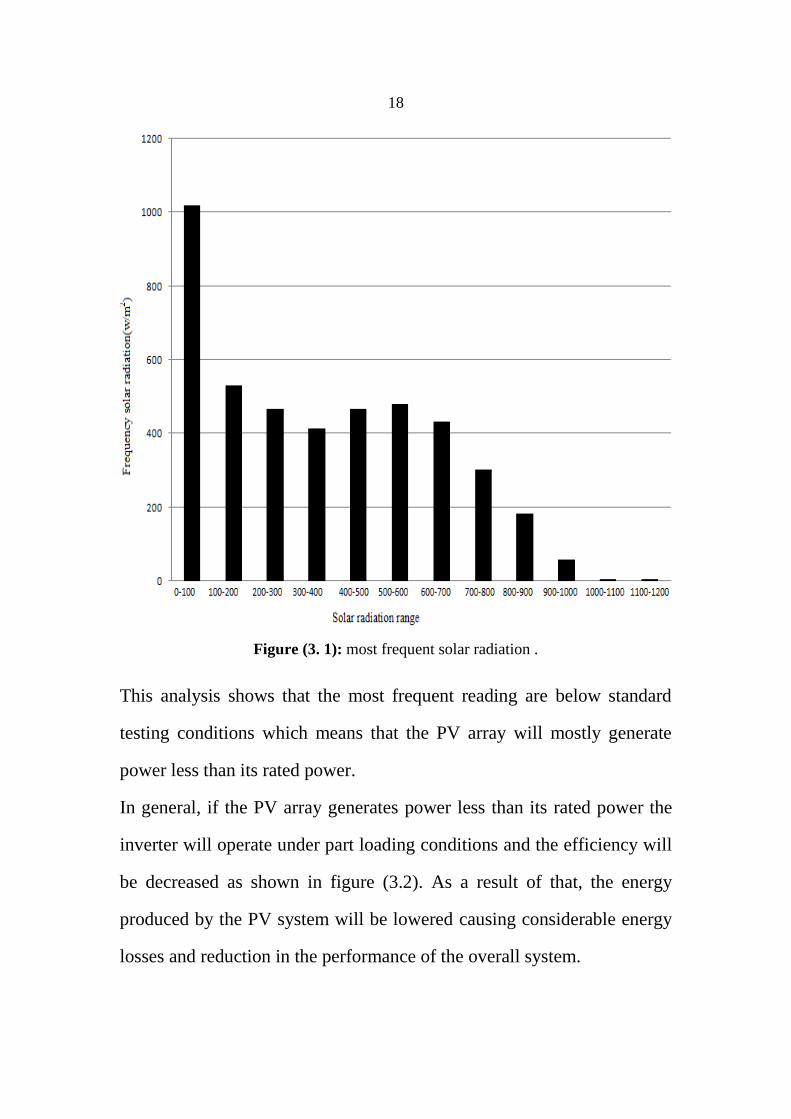
Figure (3.1) shows the distribution frequency analysis of the solar
radiation records in Palestine.
From the figure, the largest number of hours which is 1020 hours in the
year contains low solar radiation records (less than 100 w/m2) which
represents approximately 23.3% of the total readings while approximately
70.9% of the total readings (2795 hours) contain solar radiation records in
the range (100-800) w/m2. In the meanwhile, approximately about 12.4%
of the total readings (543hours) contain solar radiation records in the
range of (700-1000 w/m2) while, the lowest number of hours (12 hours)
contain solar radiation records above 1000 w/m2 which represent 0.27%
of the total readings.
18
Figure (3. 1): most frequent solar radiation .
This analysis shows that the most frequent reading are below standard
testing conditions which means that the PV array will mostly generate
power less than its rated power.
In general, if the PV array generates power less than its rated power the
inverter will operate under part loading conditions and the efficiency will
be decreased as shown in figure (3.2). As a result of that, the energy
produced by the PV system will be lowered causing considerable energy
losses and reduction in the performance of the overall system.
19
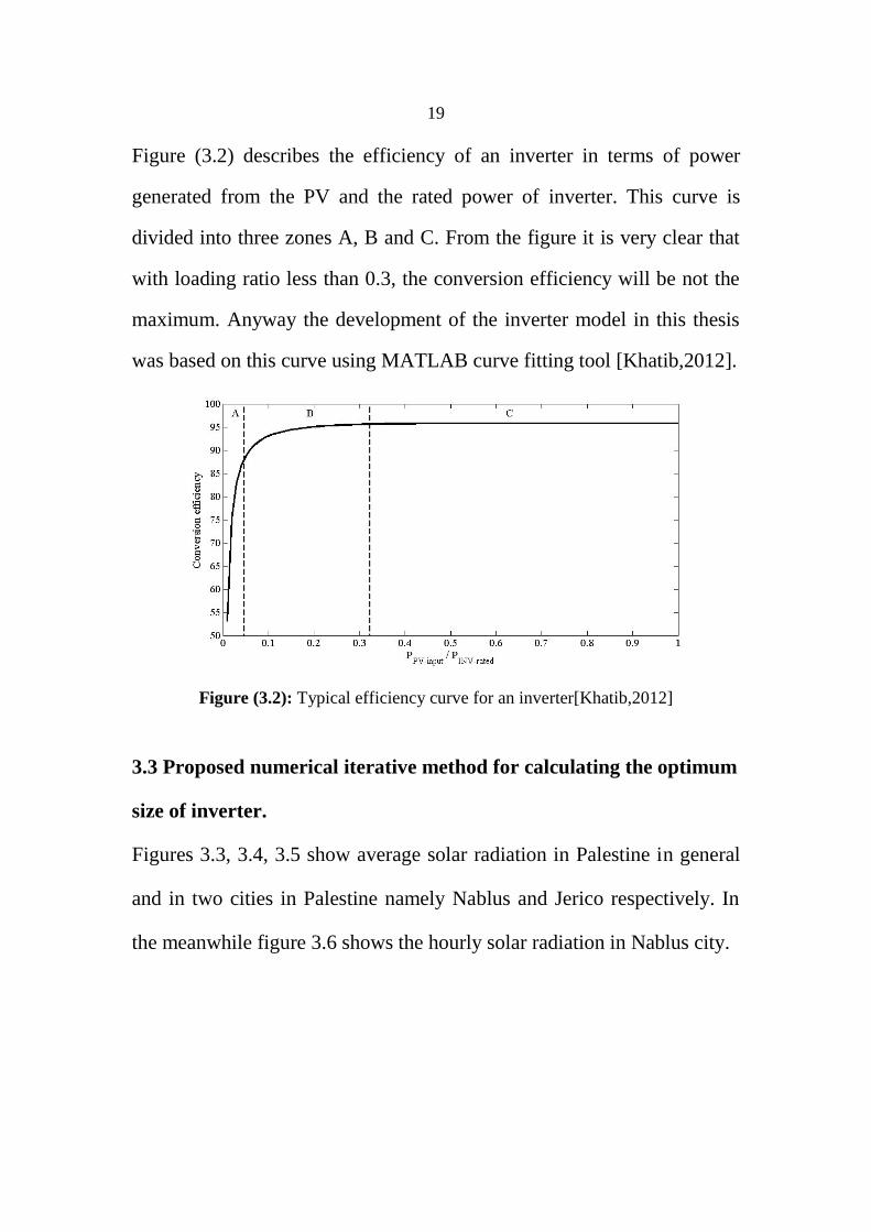
Figure (3.2) describes the efficiency of an inverter in terms of power
generated from the PV and the rated power of inverter. This curve is
divided into three zones A, B and C. From the figure it is very clear that
with loading ratio less than 0.3, the conversion efficiency will be not the
maximum. Anyway the development of the inverter model in this thesis
was based on this curve using MATLAB curve fitting tool [Khatib,2012].
Figure (3.2): Typical efficiency curve for an inverter[Khatib,2012]
3.3 Proposed numerical iterative method for calculating the optimum
size of inverter.
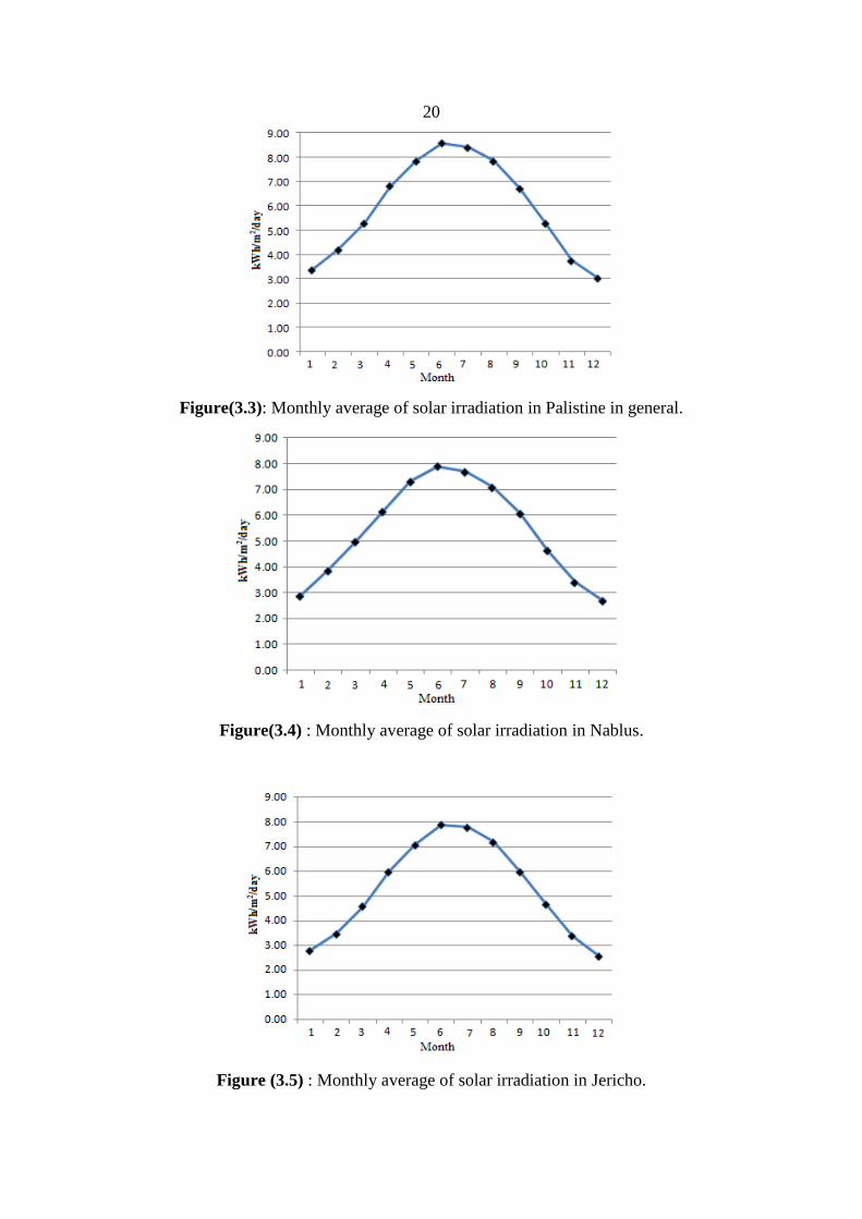
Figures 3.3, 3.4, 3.5 show average solar radiation in Palestine in general
and in two cities in Palestine namely Nablus and Jerico respectively. In
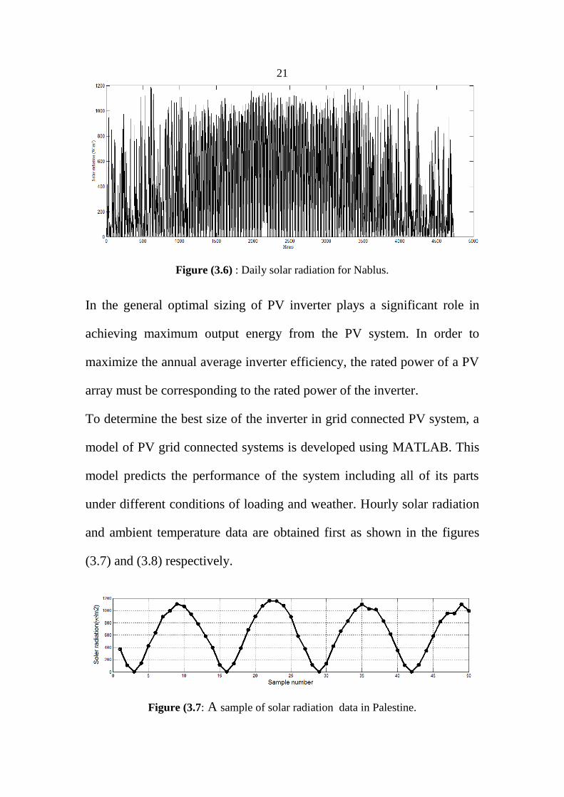
the meanwhile figure 3.6 shows the hourly solar radiation in Nablus city.
20
Figure(3.3): Monthly average of solar irradiation in Palistine in general.
Figure(3.4) : Monthly average of solar irradiation in Nablus.
Figure (3.5) : Monthly average of solar irradiation in Jericho.
21
Figure (3.6) : Daily solar radiation for Nablus.
In the general optimal sizing of PV inverter plays a significant role in
achieving maximum output energy from the PV system. In order to
maximize the annual average inverter efficiency, the rated power of a PV
array must be corresponding to the rated power of the inverter.
To determine the best size of the inverter in grid connected PV system, a
model of PV grid connected systems is developed using MATLAB. This
model predicts the performance of the system including all of its parts
under different conditions of loading and weather. Hourly solar radiation
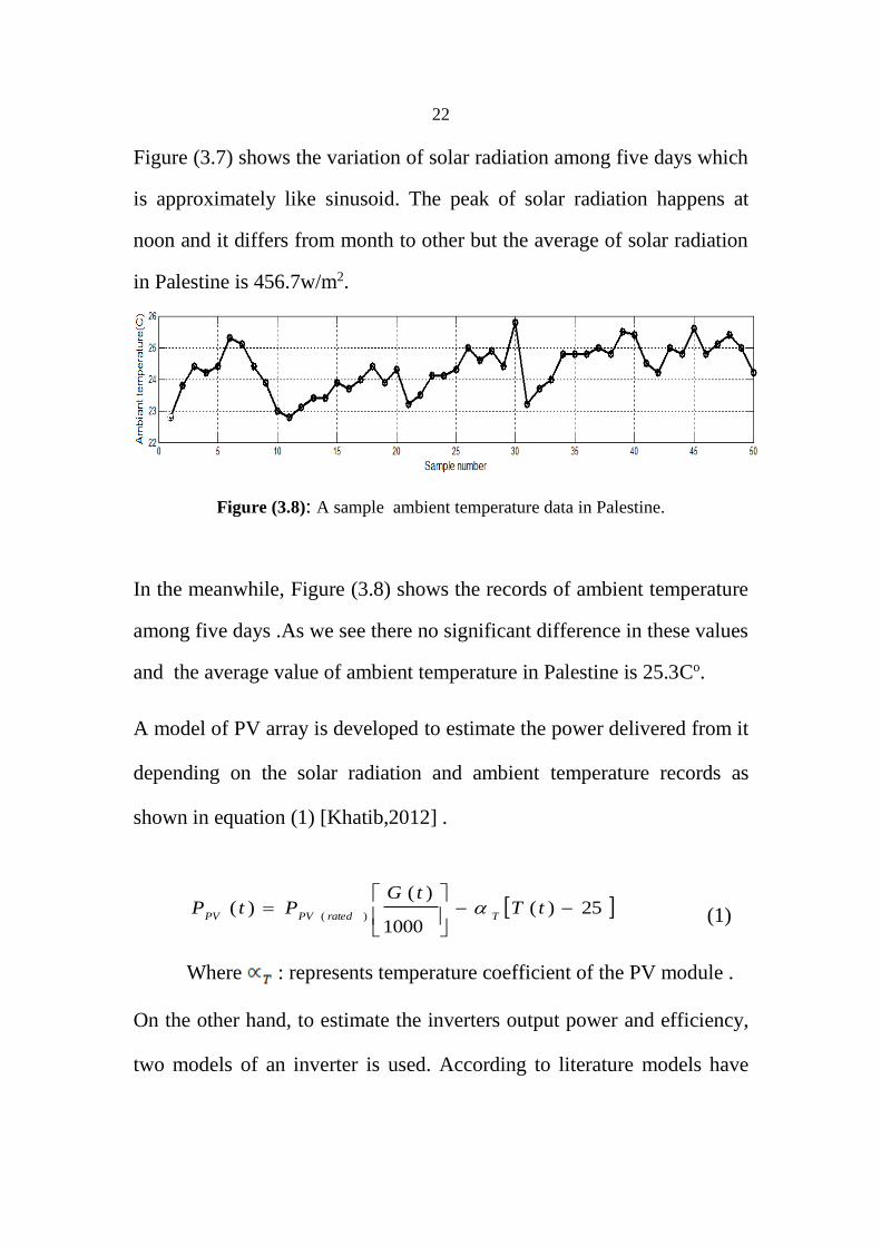
and ambient temperature data are obtained first as shown in the figures
(3.7) and (3.8) respectively.
Figure (3.7: A sample of solar radiation data in Palestine.
22
Figure (3.7) shows the variation of solar radiation among five days which
is approximately like sinusoid. The peak of solar radiation happens at
noon and it differs from month to other but the average of solar radiation
in Palestine is 456.7w/m2.
Figure (3.8): A sample ambient temperature data in Palestine.
In the meanwhile, Figure (3.8) shows the records of ambient temperature
among five days .As we see there no significant difference in these values
and the average value of ambient temperature in Palestine is 25.3Co.
A model of PV array is developed to estimate the power delivered from it
depending on the solar radiation and ambient temperature records as
shown in equation (1) [Khatib,2012] .
25)(1000
)()(
)(
tT
tGPtP
TratedPVPV (1)
Where : represents temperature coefficient of the PV module .
On the other hand, to estimate the inverters output power and efficiency,
two models of an inverter is used. According to literature models have
23
been developed in the literature. A model based on weighting of the
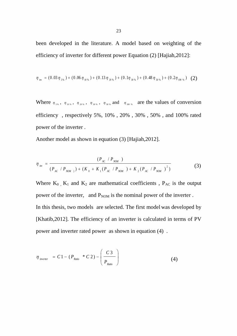
efficiency of inverter for different power Equation (2) [Hajiah,2012]:
)2.0()48.0()1.0()13.0()06.0()03.0(%100%50%30%20%10%5
inv (2)
Where %5
, %10
, %20
, %30
, %50
and %100
are the values of conversion
efficiency , respectively 5%, 10% , 20% , 30% , 50% , and 100% rated
power of the inverter .
Another model as shown in equation (3) [Hajiah,2012].
))/()/(()/(
)/(
2
210) NOMACNOMACNOMAC
NOMAC
inv
PPKPPKKPP
PP
(3)
Where K0 , K1 and K2 are mathematical coefficients , PAC is the output
power of the inverter, and PNOM is the nominal power of the inverter .
In this thesis, two models are selected. The first model was developed by
[Khatib,2012]. The efficiency of an inverter is calculated in terms of PV
power and inverter rated power as shown in equation (4) .
Ratio
Ratioinverter
P
CCPC
3)2*(1
(4)

24
Where:
inverter
ratedPV
Ratio
P
tGP
P
1000
)(*
)(
(5)
While C1, C2 and C3 are the model coefficients .
Table (3. 1) : Inverter models coefficients
C1 C2 C3
5kW 97.644 1.995 0.455
50kW 100.583 3.611 0.972
100kW 99.967 3.222 0.644
The optimum size of an inverter is represented by the ratio Rs which
represents the rated power of the PV array to the rated power of inverter
used as follows.
)(
)(
ratedinv
ratedPV
S
P
PR (6)
The second model which is considered is shown in equation (7)
10987
...654321
23
456789
pxpxpxp
xpxpxpxpxpxpxf
(7)
Where p1,p2,p3, p4,p5,p6,p7,p8,p9 and p10 are Coefficients values
p1 = 0.8744 , p2 = -13.11 , p3 = 83.94 , p4 = -299.9 p5 = 655.2
p6 = -902.6 , p7 = 781 , p8 = -410.3 , p9 = 118.4 , p10 = 82.6
and x is the PRatio

25
Figure (3.9) shows the optimization algorithm for inverter size in a grid
connected PV system. At the beginning, the PV system parameters such
as the rated power of the PV array and the temperature coefficient of the
PV module and the inverter model coefficients are obtained. The solar
radiation and ambient temperature records are used. In the iteration loop a
set of RS (from 0.5 to 5 at step equal to .01) values is proposed. The rated
power of inverter can be obtained by dividing the rated power of the PV
to each value of RS. Then the hourly PV array output is calculated using
the PV model in equation (1). Then by using the inverter model described
in equation (4) and (7) , the hourly inverter efficiency is calculated.
After that, the average yearly efficiency is calculated by dividing the
summation of the hourly inverter efficiency among the year to the
number of records and stored it in an array. The loop will be repeated
until Rs reaches its maximum value. Finally, when Rs reaches its
maximum value, a search for the maximum efficiency and its optimum
Rs is found. A curve shows the relation between Rs values and the
average efficiency is plotted and the optimum value of Rs and its
maximum efficiency are shown on this curve.
The following flowchart presents the proposed iteration method used for
determining the optimal inverter size. The iterative method which has
been described above is done using the model described in equation (4)
for an inverter with different sizes .
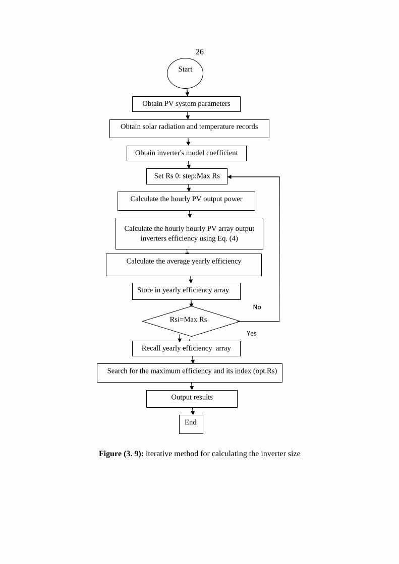
26
Figure (3. 9): iterative method for calculating the inverter size
Start
Obtain PV system parameters
Obtain solar radiation and temperature records
Obtain inverter's model coefficient
Set Rs 0: step:Max Rs
Calculate the hourly PV output power
Calculate the hourly hourly PV array output
inverters efficiency using Eq. (4)
Calculate the average yearly efficiency
Store in yearly efficiency array
Rsi=Max Rs
Recall yearly efficiency array
Search for the maximum efficiency and its index (opt.Rs)
End
Output results
Yes
No

27
3.4 Validation of thesis’s proposal :
To see the benefits of optimally sizing the inverter in grid connected
system , a comparison between having a normally select inverter (its
capacity matches to the PV array capacity) and a second system where
the inverter is optimally installed considering the sizing ratio is
considered and simulate the two system for one year time using
MATLAB for three different sizes of inverter (5 kW,50kW and 100kW) .
The two systems are simulated to calculate the total energy produced, the
average yearly efficiency and the losses.
The flow chart described in figure (3.10) shows the methodology of
calculating the energy yield of the system considering a normally
installed inverter. At the beginning, PV parameters such as the rated
power of PV array is obtained. The hourly solar radiation and ambient
temperature records are also obtained to calculate the hourly power of PV
array using equation (1). In this case avoid set the rated power of an
inverter equal to the rated power of PV . Then equation (4) and (5) are
used to calculate the hourly efficiency for the inverter. The hourly output
power from the inverter can be calculated by multiplying the hourly
efficiency of it with the hourly power of PV. The average efficiency can
then be calculated by dividing the summation of the hourly efficiency to
length of these values. The total energy produced from the PV system and
the inverter are calculated by summation the hourly power for each of
them. The losses for the whole year of this system can be calculated by
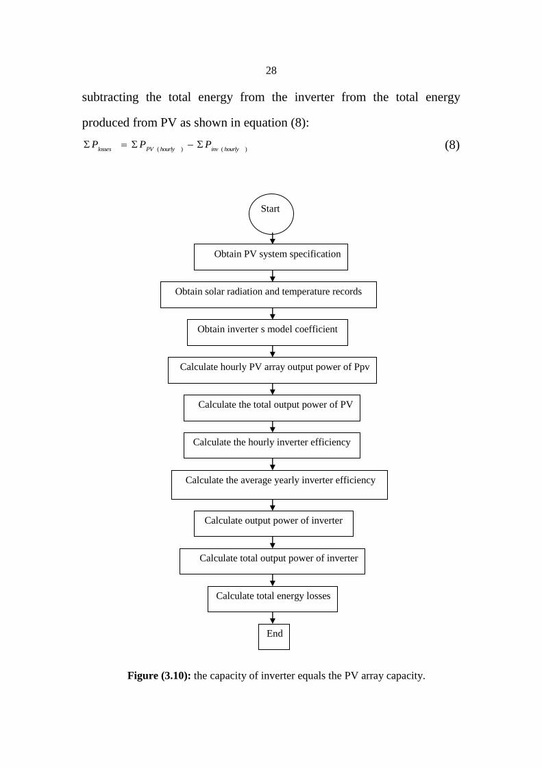
28
subtracting the total energy from the inverter from the total energy
produced from PV as shown in equation (8):
)()( hourlyinvhourlyPVlossesPPP (8)
Obtain solar radiation and temperature records
Obtain inverter s model coefficient
Calculate hourly PV array output power of Ppv
Calculate the total output power of PV
Calculate the hourly inverter efficiency
Calculate the average yearly inverter efficiency
Calculate output power of inverter
Calculate total output power of inverter
Calculate total energy losses
End
Start
Obtain PV system specification
Figure (3.10): the capacity of inverter equals the PV array capacity.
29
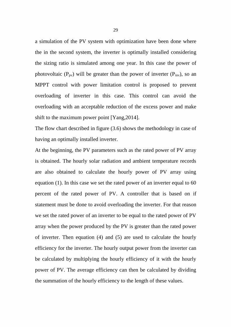
a simulation of the PV system with optimization have been done where
the in the second system, the inverter is optimally installed considering
the sizing ratio is simulated among one year. In this case the power of
photovoltaic (Ppv) will be greater than the power of inverter (Pinv), so an
MPPT control with power limitation control is proposed to prevent
overloading of inverter in this case. This control can avoid the
overloading with an acceptable reduction of the excess power and make
shift to the maximum power point [Yang,2014].
The flow chart described in figure (3.6) shows the methodology in case of
having an optimally installed inverter.
At the beginning, the PV parameters such as the rated power of PV array
is obtained. The hourly solar radiation and ambient temperature records
are also obtained to calculate the hourly power of PV array using
equation (1). In this case we set the rated power of an inverter equal to 60
percent of the rated power of PV. A controller that is based on if
statement must be done to avoid overloading the inverter. For that reason
we set the rated power of an inverter to be equal to the rated power of PV
array when the power produced by the PV is greater than the rated power
of inverter. Then equation (4) and (5) are used to calculate the hourly
efficiency for the inverter. The hourly output power from the inverter can
be calculated by multiplying the hourly efficiency of it with the hourly
power of PV. The average efficiency can then be calculated by dividing
the summation of the hourly efficiency to the length of these values.

30
The total energy produced from the PV system and the inverter are
calculated by summation the hourly power for each of them. At the end
the losses for the whole year of this system can be calculated by
subtracting the total energy from the inverter from the total energy
produced from PV as shown in equation (7).
Figure (3.11): the inverter is optimally installed according to the sizing ratio (Pinv is
60% of Ppv).
In addition, the annual yield factor and the capacity factor are used to
compare both systems. The annual yield factor (YF) in kWh/kWp is
Start
Obtain PV system specification
Obtain solar radiation and temperature records
Obtain PV system specification
Calculate hourly PV array output power of Ppv
Pinv < If Ppv out
Calculate the hourly inverter efficiency
Pinv Ppv_new =
Calculate the average yearly efficiency
Calculate output power of inverter
Losses = Ppv - Pinv
End
No
Yes
Set Pinv = Ppv/1.6
31
defined as the ratio between the annual energy output produced from the
PV system to the rated power of the PV array as shown in equation (8)
[Rampinelli,2014].
)(
)/(
)(KWpP
yearKWhEY
ratedPV
PV
F (8)
In the meanwhile, the capacity factor (CF) is defined as the ratio of the
annual yield factor to number of hours in a year. The capacity factor
evaluates the usage of the PV array:
8760
F
F
Y
C (9)
32
Chapter Four
Results and discussion
4.1 Introduction
An optimal sizing of inverter in grid connected PV system has been done.
The optimum size of inverter in grid tie PV system for Palestine is
searched using the iterative method described in chapter three by taking
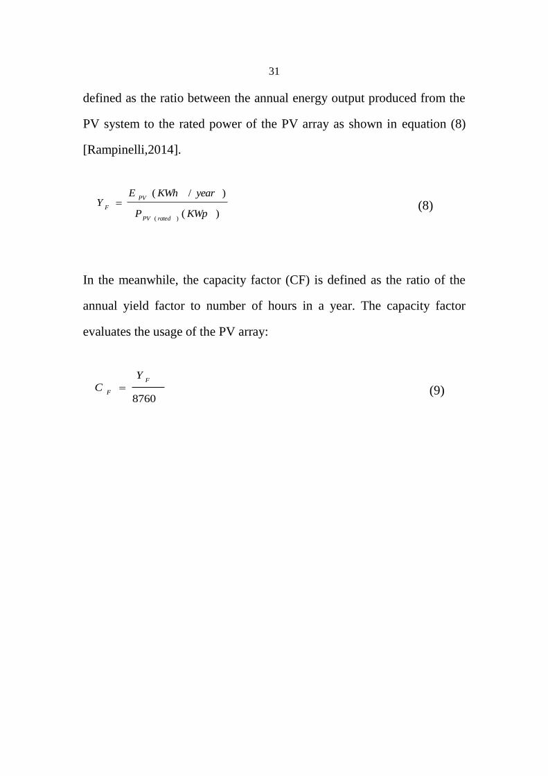
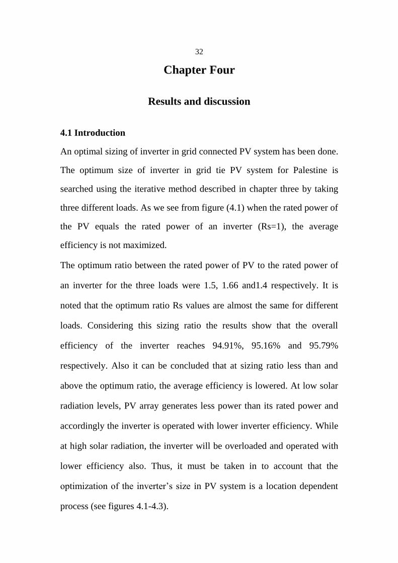
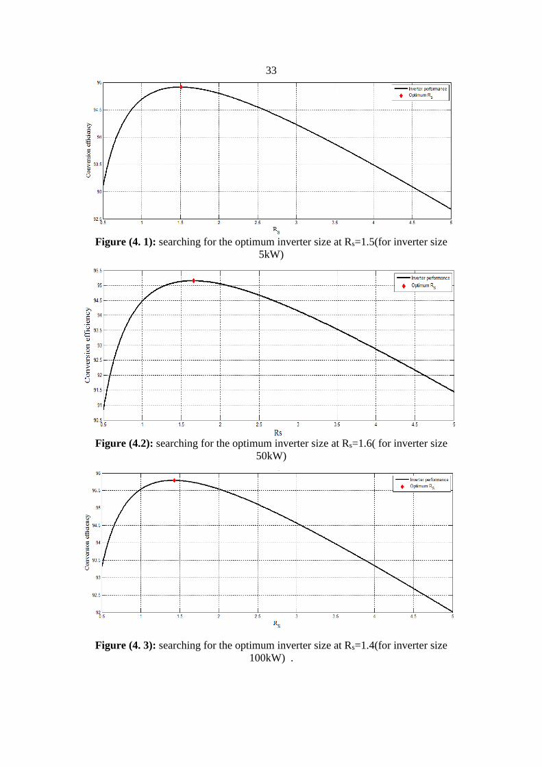
three different loads. As we see from figure (4.1) when the rated power of
the PV equals the rated power of an inverter (Rs=1), the average
efficiency is not maximized.
The optimum ratio between the rated power of PV to the rated power of
an inverter for the three loads were 1.5, 1.66 and1.4 respectively. It is
noted that the optimum ratio Rs values are almost the same for different
loads. Considering this sizing ratio the results show that the overall
efficiency of the inverter reaches 94.91%, 95.16% and 95.79%
respectively. Also it can be concluded that at sizing ratio less than and
above the optimum ratio, the average efficiency is lowered. At low solar
radiation levels, PV array generates less power than its rated power and
accordingly the inverter is operated with lower inverter efficiency. While
at high solar radiation, the inverter will be overloaded and operated with
lower efficiency also. Thus, it must be taken in to account that the
optimization of the inverter’s size in PV system is a location dependent
process (see figures 4.1-4.3).
33
Figure (4. 1): searching for the optimum inverter size at Rs=1.5(for inverter size
5kW)
Figure (4.2): searching for the optimum inverter size at Rs=1.6( for inverter size
50kW)
Figure (4. 3): searching for the optimum inverter size at Rs=1.4(for inverter size
100kW) .
34
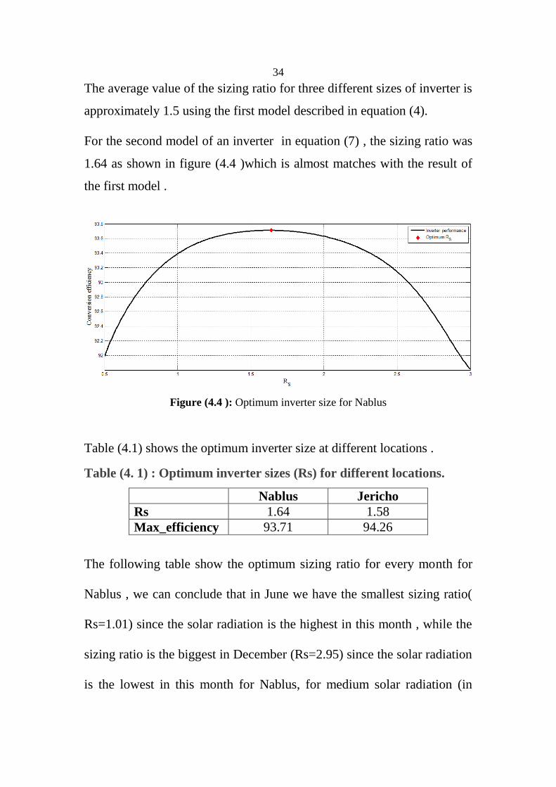
The average value of the sizing ratio for three different sizes of inverter is
approximately 1.5 using the first model described in equation (4).
For the second model of an inverter in equation (7) , the sizing ratio was
1.64 as shown in figure (4.4 )which is almost matches with the result of
the first model .
Figure (4.4 ): Optimum inverter size for Nablus
Table (4.1) shows the optimum inverter size at different locations .
Table (4. 1) : Optimum inverter sizes (Rs) for different locations.
Nablus Jericho
Rs 1.64 1.58
Max_efficiency 93.71 94.26
The following table show the optimum sizing ratio for every month for
Nablus , we can conclude that in June we have the smallest sizing ratio(
Rs=1.01) since the solar radiation is the highest in this month , while the
sizing ratio is the biggest in December (Rs=2.95) since the solar radiation
is the lowest in this month for Nablus, for medium solar radiation (in
35
September )the sizing ratio was (Rs=1.36 ) and the average sizing ratio
for Nablus was 1.64
Table (4. 2) : Monthly (Rs) and maximum efficiency.
Month Rs Max_ eff
January 2.75 92.9
February 2.19 93.5
March 1.71 93.7
April 1.27 94.5
May 1.07 94.6
June 1.01 94.82
July 1.03 94.63
August 1.11 94.56
September 1.36 94.25
October 1.88 93.91
November 2.31 93.18
December 2.95 93.35
Average 1.64 94.2
4.2 Results for the validation of the proposed methods
In order to validate the proposal of the thesis, a comparison between
having a normally inverter (its capacity equals to the PV array capacity)
and a second system where the inverter is optimally installed considering
the sizing ratio will be considered and simulate the two system for one
year time to see the total energy produced.
Case1: the capacity of inverter matches the PV array capacity
In this case a simulation of the PV system without optimization is made
36
(the capacity of the PV array is equal power of inverter) to calculate the
total energy produced, the average yearly efficiency and the losses.
Figure (4.5) shows the hourly power of PV, efficiency and power of
inverter for five days.
Figure (4.5): the solar radiation , hourly power of PV , efficiency and power of
inverter.
The hourly PV power is vary among the year since the hourly solar
radiation and temperature is changed; The output power of a PV array
increases linearly as the solar radiation increases, and therefore the hourly
efficiency will be changed since it depends on power generated from the
PV, the average yearly efficiency for this case is 94.465% .the hourly
output power of the inverter is changed accordingly. The total energy
from the inverter is 24893kwh and total losses is 1550 kWh among one
year.
37
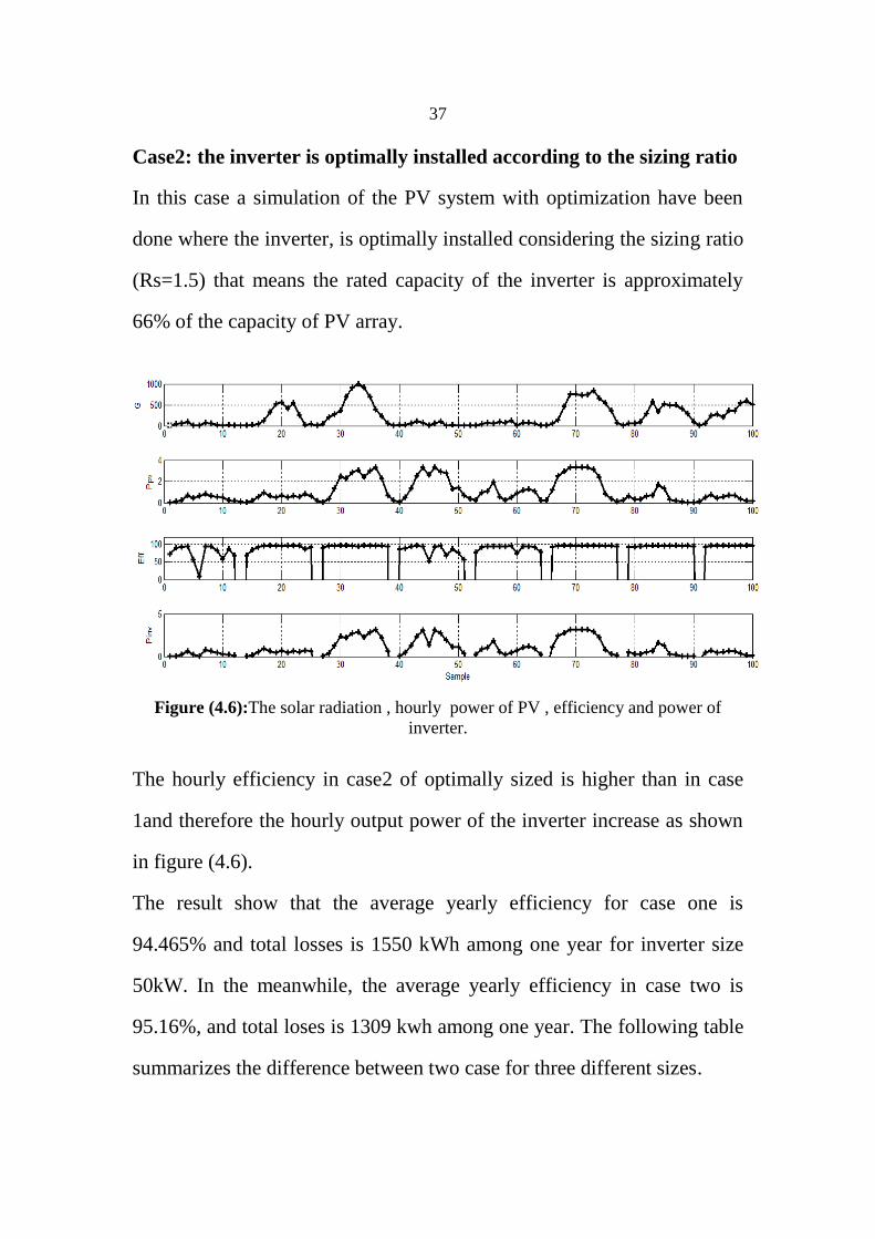
Case2: the inverter is optimally installed according to the sizing ratio
In this case a simulation of the PV system with optimization have been
done where the inverter, is optimally installed considering the sizing ratio
(Rs=1.5) that means the rated capacity of the inverter is approximately
66% of the capacity of PV array.
Figure (4.6):The solar radiation , hourly power of PV , efficiency and power of
inverter.
The hourly efficiency in case2 of optimally sized is higher than in case
1and therefore the hourly output power of the inverter increase as shown
in figure (4.6).
The result show that the average yearly efficiency for case one is
94.465% and total losses is 1550 kWh among one year for inverter size
50kW. In the meanwhile, the average yearly efficiency in case two is
95.16%, and total loses is 1309 kwh among one year. The following table
summarizes the difference between two case for three different sizes.

38
Table (4. 3) : Comparison between tow cases.
Case 1 (Without optimization)
Case2 (With optimization)
Ppv_rated(kWp) 5 50 100 5 50 100
Pinv_rated /
Ppv_rated
100 100 100 66 60 70
Rs 1 1 1 1.5 1.6 1.4
Ppv_tot 2644 2644 52889 2472 26444 50278
Average efficiency 94.68 94.46% 95.53 94.91 95.16% 95.79
Pinv_tot 2500 24893 50422 2345 25135 48115
Total Losses( kwh ) 277 2927 4716 246 1309 4186
YF (kWh / kWp) 500 497.86 504 469 502.7 481
CF (%) 5.7 5.6 5.7 5.3 5.7 5.4
From the table, it can be concluded that case 2 is better than case 1 in
terms of efficiency and energy losses. The total output of inverter in
case2 of optimally sized inverter is greater than case 1 since the
efficiency is higher and therefore the losses is lower. The annual yield
factor for optimally sized system for 50 Kw is 502.7 kWh/kWp per year,
meanwhile, the annual yield factor for normally installed inverter is
497.86 kWh/kWp per year for inverter size of 50kw. This proves that the
optimal sizing of the PV inverter has better performance when it
compared to normal installed one, since the losses is less and the average
maximum efficiency is greater .
39
Chapter Five
5.1 Conclusion
In this thesis optimal sizing of grid connected inverter of the PV systems
was carried out . solar radiation and ambient temperature for Palestine are
also obtained to develop models for photovoltaic array and inverter. The
results show that the average optimum inverter size ratio is 1.5 for
three different loads and the average maximum efficiency reaches
95.29% . A comparison between having a normally inverter (its capacity
equals to the PV array capacity ) and a second system where the inverter
is optimally installed considering the sizing ratio is considered and
simulate the two system for one year time using matlab.it is observed that
the total energy produced and the losses from case one are 24893kwh
and 1550kwh respectively whereas in case 2 are 25135 kWh and 1309
kWh respectively. From the results, it is noted that optimum sizing of PV
inverter increases the efficiency and the total energy produced and reduce
the losses. The annual yield factor for optimum sizing system is 502.7
kWh/kWp/year whereas the annual yield factor for normally installed
inverter is 497.86 kWh/kWp/year. This proves that sizing the PV inverter
has almost the best performance when compared to normal installed one.

40
5.2 Future work:
1- Simulate different models of inverter to make comparison of the
inverter efficiency performance .
2- Design a GUI in Matlab which describe mathematical modeling
and analysis of a PV system to be used as evaluating tool.
3- Making the comparison between the cases of having a normally
installed inverter and an optimally installed inverter
experimentally.
41
References
Santra, P. and Kamat, P. (2012). Mn-Doped Quantum Dot Sensitized
Solar Cells: A Strategy to Boost Efficiency over 5%. Journal of the
American Chemical Society, 134(5), pp.2508-2511.
Yasin , A. (2008). Optimal Operation Strategy and Economic
Analysis of Rural Electrification of Atouf Village by Electric
Network, Diesel Generator and Photovoltaic System. M.Sc. An-Najah
National University
khatib,T. Azah Mohamed, K.sppian and Marwan Mahmoud.(2012)."
An Iterative Method for Calculating the Optimum Size of Inverter in
PV Systems for Malaysia". ISSN 0033-2097, R. 88 NR 4a.
Keller, L. and Affolter, P. (1995). Optimizing the panel area of a
photovoltaic system in relation to the static inverter—Practical
results. Solar Energy, 55(1), pp.1-7.
Coppye.W, Maranda.W, Nir.Y, De Gheselle.L, Nijs.J(1995).:Detailed
comparison of the inverter operation of two grid connected PV
demonstration systems in Belgium. Nice, France:, pp.1881-1884.
Macagnan, M.H, Lorenzo E(1992): On the optimal size of inverters
for grid connected PV systems. Montreux, Switzerland:, pp.1167-
1170.
Jantsch, M., Schmidt H, Schmid, J., (1992).:Results of the concerted
action on power conditioning and control. Montreux, Switzerland,
pp. 1589–1593.
42
Velasco ,G., Piqué, R., F., Guinjoan ,F., Casellas and J. de la
Hoz(2010): Power sizing factor design of central inverter PV grid
connected systems: a simulation approach. Metropol Lake Resort
Ohrid, Macedonia:, pp.32-36.
Stetz, T., Kunschner, J., Braun, M. and Engel, B. (1992). Cost optimal
sizing of photovoltaic inverters influence of new grid codes and cost
reductions. Fraunhofer IWES, Koenigstor, (D-34119).
Mondol, J., Yohanis, Y. and Norton, B. (2007). The effect of low
insolation conditions and inverter oversizing on the long-term
performance of a grid-connected photovoltaic system. Progress in
Photovoltaics: Research and Applications, 15(4), pp.353-368.
Burger, B. and Rüther, R. (2006). Inverter sizing of grid-connected
photovoltaic systems in the light of local solar resource distribution
characteristics and temperature. Solar Energy, 80(1), pp.32-45.
Macêdo, W. and Zilles, R. (2007). Operational results of grid-
connected photovoltaic system with different inverter's sizing factors
(ISF). Progress in Photovoltaics: Research and Applications, 15(4),
pp.337-352.
Demoulias, C. (2010). A new simple analytical method for calculating
the optimum inverter size in grid-connected PV plants. Electric
Power Systems Research, 80(10), pp.1197-1204.
Mondol, J., Yohanis, Y. and Norton, B. (2006). Optimal sizing of
array and inverter for grid-connected photovoltaic systems. Solar
Energy, 80(12), pp.1517-1539.
43
Notton ,G., Lazarov ,V. , Stoyanova ,L. (2010):" Optimal sizing of a
grid-connected PV system for various PV module technologies and
inclinations, inverter efficiency characteristics and
locations,Renewable Energy 35 (2010) 541–554 .
Kornelakis ,A., (2010)." Optimization for the optimal design of
photovoltaic grid-connected systems" , Solar Energy 84 , 2022–2033.
Rampinelli, G., Krenzinger, A. and Chenlo Romero, F. (2014).
Mathematical models for efficiency of inverters used in grid
connected photovoltaic systems. Renewable and Sustainable Energy
Reviews, 34, pp.578-587.
Hajiah, A., Khatib, T., Sopian, K. and Sebzali, M. (2012).
Performance of Grid-Connected Photovoltaic System in Two Sites in
Kuwait. International Journal of Photoenergy, 2012, pp.1-7.
Yang, Y., Wang, H., Blaabjerg, F. and Kerekes, T. (2014). A Hybrid
Power Control Concept for PV Inverters With Reduced Thermal
Loading. IEEE Transactions on Power Electronics, 29(12),
pp.6271-6275.
Kymakis, E., Kalykakis, S. and Papazoglou, T. (2009). Performance
analysis of a grid connected photovoltaic park on the island of Crete.
Energy Conversion and Management, 50(3), pp.433-438.
44
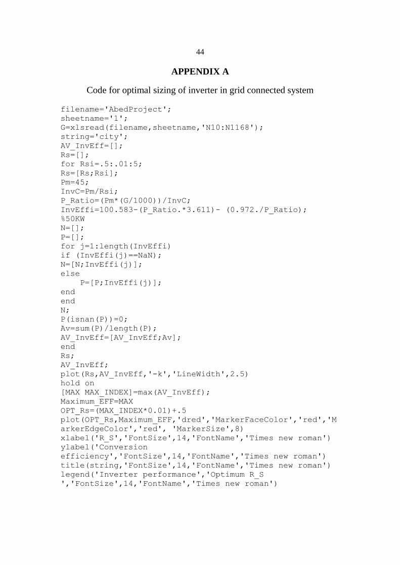
APPENDIX A
Code for optimal sizing of inverter in grid connected system
filename='AbedProject';
sheetname='1';
G=xlsread(filename,sheetname,'N10:N1168');
string='city';
AV_InvEff=[];
Rs=[];
for Rsi=.5:.01:5;
Rs=[Rs;Rsi];
Pm=45;
InvC=Pm/Rsi;
P_Ratio=(Pm*(G/1000))/InvC;
InvEffi=100.583-(P_Ratio.*3.611)- (0.972./P_Ratio);
%50KW
N=[];
P=[];
for j=1:length(InvEffi)
if (InvEffi(j)==NaN);
N=[N;InvEffi(j)];
else
P=[P;InvEffi(j)];
end
end
N;
P(isnan(P))=0;
Av=sum(P)/length(P);
AV_InvEff=[AV_InvEff;Av];
end
Rs;
AV_InvEff;
plot(Rs,AV_InvEff,'-k','LineWidth',2.5)
hold on
[MAX MAX_INDEX]=max(AV_InvEff);
Maximum_EFF=MAX
OPT_Rs=(MAX_INDEX*0.01)+.5
plot(OPT_Rs,Maximum_EFF,'dred','MarkerFaceColor','red','M
arkerEdgeColor','red', 'MarkerSize',8)
xlabel('R_S','FontSize',14,'FontName','Times new roman')
ylabel('Conversion
efficiency','FontSize',14,'FontName','Times new roman')
title(string,'FontSize',14,'FontName','Times new roman')
legend('Inverter performance','Optimum R_S
','FontSize',14,'FontName','Times new roman')
45
APPENDIX B
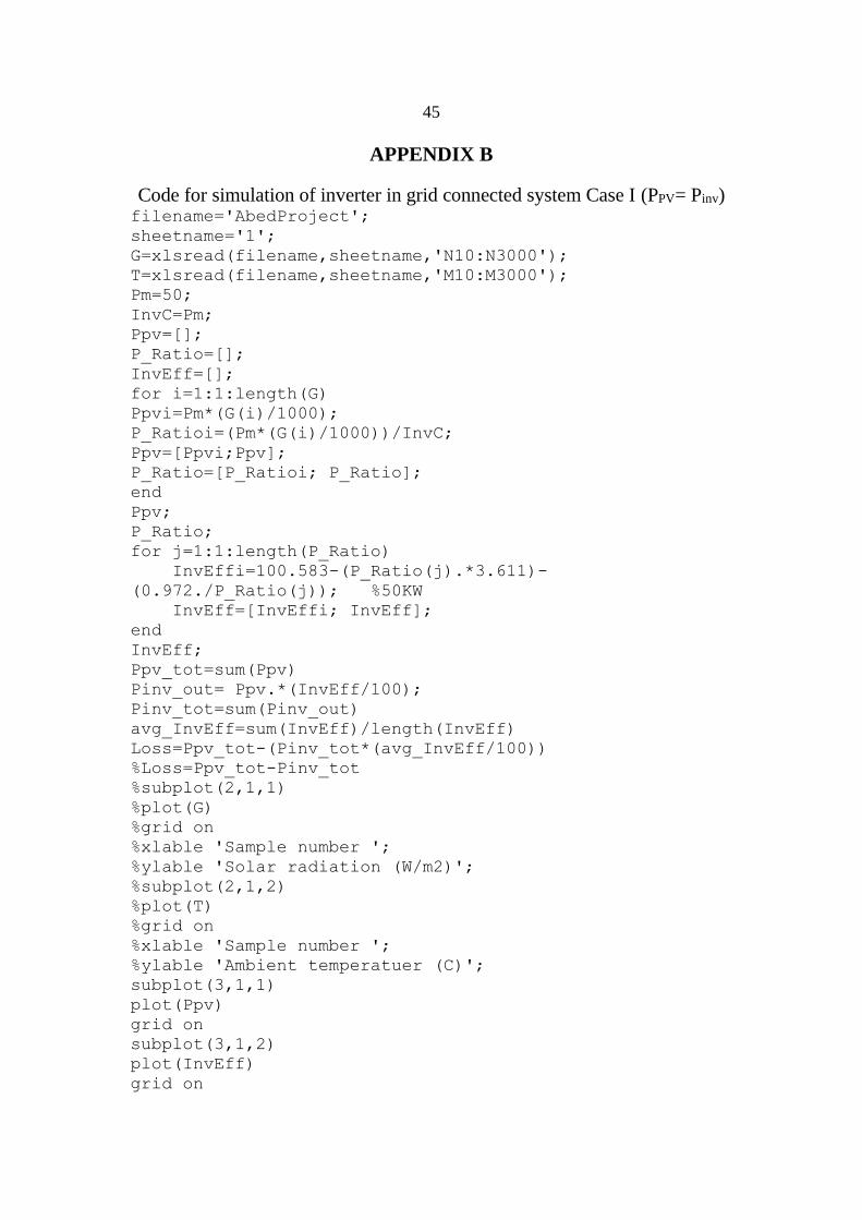
Code for simulation of inverter in grid connected system Case I (PPV= Pinv) filename='AbedProject';
sheetname='1';
G=xlsread(filename,sheetname,'N10:N3000');
T=xlsread(filename,sheetname,'M10:M3000');
Pm=50;
InvC=Pm;
Ppv=[];
P_Ratio=[];
InvEff=[];
for i=1:1:length(G)
Ppvi=Pm*(G(i)/1000);
P_Ratioi=(Pm*(G(i)/1000))/InvC;
Ppv=[Ppvi;Ppv];
P_Ratio=[P_Ratioi; P_Ratio];
end
Ppv;
P_Ratio;
for j=1:1:length(P_Ratio)
InvEffi=100.583-(P_Ratio(j).*3.611)-
(0.972./P_Ratio(j)); %50KW
InvEff=[InvEffi; InvEff];
end
InvEff;
Ppv_tot=sum(Ppv)
Pinv_out= Ppv.*(InvEff/100);
Pinv_tot=sum(Pinv_out)
avg_InvEff=sum(InvEff)/length(InvEff)
Loss=Ppv_tot-(Pinv_tot*(avg_InvEff/100))
%Loss=Ppv_tot-Pinv_tot
%subplot(2,1,1)
%plot(G)
%grid on
%xlable 'Sample number ';
%ylable 'Solar radiation (W/m2)';
%subplot(2,1,2)
%plot(T)
%grid on
%xlable 'Sample number ';
%ylable 'Ambient temperatuer (C)';
subplot(3,1,1)
plot(Ppv)
grid on
subplot(3,1,2)
plot(InvEff)
grid on

46
APPENDIX C
Code for simulation of inverter in grid connected system Case I
(PPV= 1.66Pinv) filename='AbedProject';
sheetname='1';
G=xlsread(filename,sheetname,'N10:N1168');
Pm=50;
InvC=Pm/1.66;
Ppv=[];
P_Ratio=[];
InvEff=[];
for i=1:1:length(G)
Ppvi=Pm*(G(i)/1000);
if Ppvi>InvC
Ppvi=InvC;
end
P_Ratioi=(Pm*(G(i)/1000))/InvC;
Ppv=[Ppvi;Ppv];
P_Ratio=[P_Ratioi; P_Ratio];
end
Ppv;
P_Ratio;
for j=1:1:length(P_Ratio)
InvEffi=100.583-(P_Ratio(j).*3.611)- (0.972./P_Ratio(j));
%50KW
InvEff=[InvEffi; InvEff];
end
InvEff;
Ppv_tot=sum(Ppv)
Pinv_out= Ppv.*(InvEff/100);
Pinv_tot=sum(Pinv_out)
avg_InvEff=sum(InvEff)/length(InvEff)
Loss=(Ppv_tot-(Pinv_tot*(avg_InvEff/100)))
subplot(3,1,1)
plot(Ppv)
grid on
subplot(3,1,2)
plot(InvEff)
grid on
%xlable 'Sample number' ;
%ylable 'efficiency';
subplot(3,1,3)
plot(Pinv_out)
grid on

جامعة النجاح الوطنية
كلية الدراسات العليا
وئية المرتبطة تصميم العواكس في أنظمة الخلايا الكهروض
ى/ دراسة حالة لفلسطينبالشبكة بطريقة مثل
إعداد
علي أحمد علي محمد
إشراف
تامر خطيبد.
ةالطاق هندسةدرجة الماجستير في الحصول على قدمت هذه الأطروحة استكمالا لمتطلبات
.لسطينف نابلس، ،الوطنية النجاح جامعة، العليا الدراسات بكليةافستهلاك ترشيدو النظيفة
2017

ب
لة ة حاى/ دراسلتصميم العواكس في أنظمة الخلايا الكهروضوئية المرتبطة بالشبكة بطريقة مث
لفلسطين
إعداد
علي أحمد علي محمد
إشراف
تامر خطيبد.
الملخص
لشمسية يا اانظمة الخلااختيار الحجم الامثل للعاكس الموصول على الشبكة في تم الرسالة في هذه
يا ية للخلاالاسم تم اختيار نسبة التحجيم الامثل للعاكس والذي يمثل نسبة القدرةفي فلسطين ، حيث
ةاعمل محاكم وت ، ولثلاثة مواقع مختلفة لثلاثة أحمال مختلفة الشمسية الى القدرة الاسمية للعاكس
عاكس الماتلاب لمصفوفة الخلايا الشمسية والعاكس لحساب معدل كفاءة ال برنامج باستخدام
ن حاكاة اأظهرت نتائج الم، حيث الشمسي ودرجة الحرارة في فلسطين باستخدام بيانات الاشعاع
1.5سبة التحجيم الامثل للعاكس هي ن
ية ا الشمسللخلاي للعاكس مع القدرة الاسمية ية تم عمل مقارنة بين نظام مساواة القدرة الاسموكذلك
وتم، اعليه ونظام اخر تم فيه استخدام الحجم الامثل للعاكس حسب نسبة التحجيم التي تم الحصول
:لتالية ا تائجالماتلاب وتم الحصول على الن برنامج عمل محاكاة للنظامين على مدار سنة باستخدام
اط في وكيلو 1550كيلوواط في الساعة و 24893للنظام الاول كانت الطاقة المنتجة والخسائر
يلوواط في ك 25135بينما للنظام الثاني كانت الطاقة المنتجة والخسائر الساعة على التوالي .
كيلو واط في الساعة على التوالي . 1309الساعة و
اط في الساعة كيلو و 497.86قيمته للنظام الاول تللنظامين ,فكان وتم حساب عامل العائد السنوي
يلو واط من قدرة ك 502.7لكل كيلو واط من قدرة الخلايا في السنة وللنظام الثاني كانت قيمة العائد
. الخلايا في الساعة لكل كيلو واط في السنة