An ISS Small Gain Theorem for General Networks

Sergey Dashkovskiy Bjorn S. Ruffer Fabian R. Wirth

December 20, 2007

Abstract

We provide a generalized version of the nonlinear small gain theorem for the case of morethan two coupled input-to-state stable (ISS) systems. For this result the interconnection gainsare described in a nonlinear gain matrix and the small gain condition requires bounds on theimage of this gain matrix. The condition may be interpreted as a nonlinear generalization ofthe requirement that the spectral radius of the gain matrix is less than one. We give someinterpretations of the condition in special cases covering two subsystems, linear gains, linearsystems and an associated lower-dimensional discrete time dynamical system.

Keywords: Interconnected systems input-to-state stability small gain theorem large-scalesystems monotone maps

1 Introduction

Stability is one of the fundamental concepts in the analysis and design of nonlinear dynamicalsystems. In particular, the notions of input-to-state stability (ISS) and nonlinear gains haveproved to be efficient tools for the qualitative description of stability of nonlinear control systems.There are different equivalent formulations of ISS: In terms of KL and K∞ functions (see below),via Lyapunov functions, as an asymptotic stability property combined with asymptotic gains, andothers, see [27]. A more quantitative but equivalent formulation, which captures the long termdynamic behavior of the system, is the notion of input-to-state dynamical stability (ISDS), see [9].

One of the interesting properties in the study of ISS systems is that under certain conditionsinput-to-state stability is preserved if ISS systems are connected in cascades or feedback loops. Inthis paper we generalize the existing results in this area. In particular, we obtain a general con-dition that guarantees input-to-state stability of a general system described as an interconnectionof several ISS subsystems.

The earliest interconnection result on ISS systems states that cascades of ISS systems are againISS, see e.g., [25, 24, 26]. Furthermore, small gain theorems for the case of two ISS systems ina feedback interconnection have been obtained in [9, 14, 13]. These results state in one way oranother that if the composition of the gain functions of ISS subsystems is smaller than the identity,then the overall system is ISS.

The papers [9, 14, 13] use different approaches to the formulation of small gain conditions thatyield sufficient stability criteria: In [14] the proof is trajectory-based and uses properties of KL

and K∞ functions. This approach requires that the composition of the gains is smaller than theidentity in a robust sense, see below for the precise statement. We show in Example 5.1 that withinthe context of the summation formulation of ISS the robustness condition cannot be weakened.The ISS result of [14] will turn out to be special cases of our main result. That paper also coverspractical ISS results, which we do not treat here. An ISS-Lyapunov function for the feedbacksystem is constructed in [13] as some combination of the corresponding ISS-Lyapunov functions ofboth subsystems. The key assumption of the proof in that paper is that the gains are provided interms of the max-formulation of ISS, by which the authors need not resort to a robust version ofthe small gain condition. The proof of the small gain theorem in [9] is based on the ISDS propertyand conditions for asymptotic stability of the feedback loop without inputs are derived.

1

General stability conditions for large scale interconnected systems have been obtained by va-rious authors in other contexts. In [20] sufficient conditions for the asymptotic stability of acomposite system are stated in terms of the negative definiteness of some test matrix. This matrixis defined through the given Lyapunov functions of the interconnected subsystems. Similarly, in[22] conditions for the stability of interconnected systems in terms of Lyapunov functions of theindividual systems are obtained.

In [23] Siljak considers structural perturbations and their effects on the stability of compositesystems using Lyapunov theory. The method is to reduce each subsystem to a one-dimensional one,such that the stability properties of the reduced representation imply the same stability propertiesof the original interconnected system. In some cases the lower dimensional representation givesrise to an interconnection matrix W , such that quasi dominance or negative definiteness of W

yield asymptotic stability of the composite system.In [32] small gain type theorems for general interconnected systems with linear gains can be

found. These results are of the form that the spectral radius of a gain matrix should be less thanone to conclude stability. The result obtained here may be regarded as a nonlinear generalizationin the same spirit.

In [30] Teel gives a small gain theorem for systems with outputs satisfying an ISS-relatedstability property and having saturated interconnections. In the paper it is also shown how thisresult may be used in a large variety of specific control applications. In [31] Razumikhin-typetheorems for functional differential equations are derived, which are based on the ISS small gaintheorems in [14] and [30].

In this paper we consider a system that consists of two or more ISS subsystems. We provideconditions by which the stability question of the overall system can be reduced to considerationof stability of the subsystems. We choose an approach using asymptotic gains and global stabilityto prove the ISS stability result for general interconnected systems. The generalized small gaincondition we obtain is, that for some monotone operator Γ related to the gains of the individualsystems the condition

Γ(s) 6≥ s (1)

holds for all s ≥ 0, s 6= 0 (in the sense of the component-wise ordering of the positive orthant).We discuss interpretations of this condition in Section 5.

In [4, 5, 6, 7] the authors prove that condition (1) is also sufficient for the existence of anISS Lyapunov function for interconnections of ISS subsystems. An explicit construction of thisLyapunov function in terms of the Lyapunov functions of the subsystems is described and anumerical algorithm for the construction is provided.

While the general problem of establishing ISS for networks of ISS systems can be approachedby repeated application of the cascade property and the known small gain theorem, in general thiscan be cumbersome and it is by no means obvious in which order subsystems have to be chosento proceed in such an iterative manner. Hence an extension of the known small gain theorem tolarger interconnections is needed. In this paper we obtain this extension for the general case.

The paper is organized as follows. In Section 2 notation and necessary concepts are introduced.The problem is stated in Section 3. In Section 4 we prove the main result, which generalizes theknown small gain theorem, and consider the special case of linear gains. In Section 5 the smallgain condition of the main result is discussed and we show in which way it may be interpreted asan extension of the linear condition that the spectral radius of the gain matrix has to be less thanone. It is shown that the small gain condition is intimately related to the stability of a discretetime monotone dynamical system defined using the gain matrix. Section 6 concludes this work.In Appendix A we recall some relations between non-negative matrices and directed graphs.

2

2 Preliminaries

Notation By xT we denote the transpose of a vector x ∈ Rn. In the following R+ := [0,∞).For x, y ∈ Rn, we use the standard partial order induced by the positive orthant. It is given by

x ≥ y ⇔ xi ≥ yi, i = 1, . . . , n , and x > y ⇔ xi > yi, i = 1, . . . , n. (2)

By Rn+ we denote the positive orthant x ∈ Rn : x ≥ 0.

For nonempty index sets I, J ⊂ 1, . . . , n we denote by #I the number of elements of I andby yI the restriction

yI := (yi)i∈I

for vectors y ∈ Rn+. Let PI denote the projection of Rn

+ onto R#I+ mapping y to yI , and RJ the

anti-projection R#J+ → Rn

+, defined by

x 7→#J∑

k=1

xkejk,

where ekk=1,...,n denotes the standard basis of Rn and J is

J = j1, . . . , j#J, with jk < jk+1, k = 1, . . . ,#J − 1.

This allows to define the restriction AIJ : R#J+ → R#I

+ of a mapping A : Rn+ → Rn

+ byAIJ = PI A RJ .

For a function v : R+ → Rm we define its restriction to the interval [s1, s2] by

v[s1,s2](t) :=

v(t) if t ∈ [s1, s2],

0 otherwise.

Definition 2.1 (i) A function γ : R+ → R+ is said to be of class K if it is continuous, strictlyincreasing and γ(0) = 0. It is of class K∞ if, in addition, it is proper, i.e., unbounded.

(ii) A function β : R+ × R+ → R+ is said to be of class KL if, for each fixed t, the functionβ(·, t) is of class K and, for each fixed s, the function β(s, ·) is non-increasing and tends to zerofor t → ∞.

Let | · | denote some norm in Rn, and let in particular |x|max = maxi |xi| be the maximum norm.The essential supremum norm on essentially bounded functions defined on R+ is denoted by ‖·‖∞.

Stability concepts Consider a system

x = f(x, u), x ∈ RN , u ∈ RM , (3)

such that for all initial values ξ and all essentially bounded measurable inputs u unique solutionsexist for all positive times. We denote these solutions by x(·; ξ, u).

Definition 2.2 (input-to-state stability) The system (3) is called input to state stable (ISS),if there exist functions β of class KL and γ of class K, such that the inequality

|x(t; ξ, u)| ≤ β(|ξ|, t) + γ(||u||∞)

holds for all t ≥ 0, ξ ∈ RN , u : R+ → RM measurable and essentially bounded.

Definition 2.3 (asymptotic gain) System (3) has the asymptotic gain (AG) property, if thereexists γ ∈ K∞, such that for all initial states ξ ∈ RN and all u(·) ∈ L∞([0,∞); RM ) the estimate

lim supt→∞

|x(t, ξ, u)| ≤ γ(||u||∞) (4)

holds.

3

The asymptotic gain property states, that every trajectory must ultimately stay not far from zero,depending on the magnitude of ‖u‖∞.

Note that (4) is equivalent to

lim supt→∞

|x(t, ξ, u)| ≤ γ(ess. lim supt→∞|u(t)|) = ess. lim supt→∞γ(|u(t)|), (5)

see [27].

Definition 2.4 (global stability) System (3) has the global stability (GS) property, if thereexist σ1, σ2 ∈ K∞, such that for all initial states ξ ∈ RN , all t ≥ 0, and all u(·) ∈ L∞([0,∞); RM )the estimate

|x(t, ξ, u)| ≤ σ1(|ξ|) + σ2(||u||∞) (6)

holds.

Definition 2.5 The system (3) is said to be globally asymptotically stable at zero (0-GAS), ifthere exists a β ∈ KL, such that for all initial conditions ξ ∈ RN

|x(t; ξ, 0)| ≤ β(|ξ|, t). (7)

Thus 0-GAS holds, if, when the input u is set to zero, the system (3) is globally asymptoticallystable at x∗ = 0.

By a result of Sontag and Wang [27] the asymptotic gain property and global asymptoticstability at 0 together are equivalent to ISS.

3 System interconnection

Consider n interconnected control systems given by

x1 = f1(x1, . . . , xn, u)...

xn = fn(x1, . . . , xn, u)

(8)

where xi ∈ RNi , u ∈ RM and fi : RPn

j=1Nj+M → RNi is continuous and for all r ∈ R+ it is locally

Lipschitz continuous in x = (xT1 , . . . , xT

n )T uniformly in u for |u| ≤ r.

Here xi is the state of the ith subsystem, and u is considered as an external control variable.Without loss of generality we may assume to have the same input for all systems, since we may

consider u as partitioned u = (u1, . . . , un), such that each ui is the input for subsystem i only.Then each fi is of the form fi(. . . , u) = fi(. . . , Pi(u)) = fi(. . . , ui) with some projection Pi.

If we consider individual systems, we treat the state xj , j 6= i as an independent input forxi. Thus, we call the i-th subsystem of (8) ISS, if there exist functions βi of class KL andγij , γi ∈ K ∪ 0 with γii = 0, such that the solution xi(t) starting at xi(0) satisfies

|xi(t)| ≤ βi(|xi(0)|, t) +n∑

j=1

γij(||xj [0,t]||∞) + γi(||u||∞) (9)

for all t ≥ 0. We write ΓISS = (γij). The functions γij and γi are called (nonlinear) gains.We also need GS and AG definitions for the subsystems:Subsystem i of (8) is AG, if there exist γij , γi,∈ K∞ ∪ 0, γii = 0, i, j = 1, . . . , n, such that

lim supt→∞

|xi(t, ξ;xj(·), j 6= i, u(·))| ≤∑

j

γij(||xj ||∞) + γi(||u||∞), (10)

4

and it is GS, if there exist γ1i, σ2ij , σ3i ∈ K∞ ∪ 0, i, j = 1, . . . , n, such that

|xi(t, ξ;xj(·), j 6= i, u(·))| ≤ σ1i(|ξi|) +∑

j

σ2ij(||xj ||∞) + γ3i(||u||∞), (11)

where both (10) and (11) are supposed to hold for all i = 1, . . . , n, ξi ∈ RNi ; u(·) ∈ L∞([0,∞); RM )and xj(·) ∈ L∞([0,∞); RNj ) for all j 6= i and all t ≥ 0.

We denote ΓAG = (γij)ni,j=1 and ΓGS = (σ2ij)

ni,j=1. Let Γ be one of ΓISS ,ΓAG, or ΓGS . This

matrix is referred to as gain matrix.Note that Γ defines in a natural way a map Γ : Rn

+ → Rn+ by

Γ(s1, . . . , sn)T :=

n∑

j=1

γ1j(sj), . . . ,

n∑

j=1

γnj(sj)

T

(12)

for s = (s1, . . . , sn)T ∈ Rn+. Note that by the properties of γij for s1, s2 ∈ Rn

+ we have theimplication

s1 ≥ s2 ⇒ Γ(s1) ≥ Γ(s2), (13)

so that Γ defines a monotone operator on Rn+.

For vector functions x = (xT1 , . . . , xT

n )T : R+ → RN1+...+Nn such that xi : R+ → RNi , i =1, . . . , n, and times 0 ≤ t1 ≤ t2, t ≥ 0 we define

x[t1,t2]

:=

‖x1,[t1,t2]‖∞...

‖xn,[t1,t2]‖∞

∈ Rn

+ and

x(t)

:=

|x1(t)|...

|xn(t)|

∈ Rn

+ .

For u(·) ∈ L∞([0,∞); RM ), finite times t ≥ 0, and for s ∈ Rn+ we introduce the abbreviating

notation

γ(‖u‖∞) :=

γ1(‖u‖∞)...

γn(‖u‖∞)

∈ Rn

+ and β(s, t) :=

β1(s1, t)...

βn(sn, t)

,

where γ1, . . . , γn come from (9) or (10) and βi from (9).Now we can rewrite the ISS conditions (9) of the subsystems in a vectorized form for t ≥ 0 as

x(t)

≤ β(

x(0)

, t) + ΓISS(

x[0,t]

) + γ(‖u‖∞). (14)

The AG conditions now reads

lim supt→∞

x(t)

≤ ΓAG(

x[0,t]

) + γ(‖u‖∞), (15)

where this time γ denotes the vector [γ1, . . . , γn]T corresponding to (10).For the GS assumption we obtain

x(t)

≤ σ1(ξ

) + ΓGS(

x[0,t]

) + γ3(‖u‖∞), (16)

where σ1(ξ

) = (σ11(|ξ1|), . . . , σ1n(|ξn|))T and γ3(‖u‖∞) = (γ31(‖u‖∞), . . . , γ3n(‖u‖∞))T .

Assuming each of the subsystems of (8) to be ISS, we are interested in conditions guaranteeingthat the whole system defined by x = (xT

1 , . . . , xTn )T , f = (fT

1 , . . . , fTn )T and

x = f(x, u) (17)

is ISS (from u to x).

5

Remark 3.1 (Additional Preliminaries) We also need some notation from lattice theory, cf.[28] for example.

Let (Rn+, sup, inf) be the lattice given by the standard partial order defined by (2). Here sup

denotes the supremum and inf denotes the infimum with respect to the partial order. With thisnotation the upper limit for bounded functions s : R+ → Rn

+ is defined by

lim supt→∞

s(t) := inft≥0

supτ≥t

s(τ).

We will need the following property.

Lemma 3.2 Let s : R+ → Rn+ be continuous and bounded. Then

lim supt→∞

s(t) = lim supt→∞

s[t/2,∞)

.

Proof Let lim supt→∞ s(t) =: a ∈ Rn+ and lim supt→∞

s[t/2,∞)

=: b ∈ Rn+. For every

ε ∈ Rn+, ε > 0 (component-wise!) there exist ta, tb ≥ 0 such that

∀ t ≥ ta : supt≥ta

s(t) ≤ a + ε and ∀ t ≥ tb : supt≥tb

s[t/2,∞)

≤ b + ε. (18)

Clearly we haves(t) ≤

s[t/2,∞)

for all t ≥ 0, i.e., a ≤ b. On the other hand s(τ) ≤ a + ε for τ ≥ t implies

s[τ/2,∞)

≤ a + ε forτ ≥ 2t, i.e., b ≤ a.

4 Main results

In the following subsection we present a nonlinear version of the small gain theorem for networks.In Subsection 4.5 we restate this theorem for the case when the gains are linear functions.

4.1 AG, GS, and ISS small gain theorems

We introduce the following notation. For αi ∈ K∞, i = 1, . . . , n define a diagonal operatorD : Rn

+ → Rn+ by

D(s1, . . . , sn)T :=

(Id + α1)(s1)...

(Id + αn)(sn)

. (19)

We say that a gain matrix Γ satisfies the small gain condition, if there exists an operator D asin (19), such that for all s ∈ Rn

+, s 6= 0 we have

Γ D(s) := Γ(D(s)) s. (20)

For short we just write Γ D id. This condition can equivalently be stated as: There has to beat least one i ∈ 1, . . . , n, such that the ith component of Γ D decreases, i.e., Γ(D(s))i < si.Note that Γ D id if and only if D Γ id.

Theorem 4.1 (small gain global stability theorem) Assume each subsystem of (8) is GS.If ΓGS satisfies the small gain condition (20), then (17) possesses the global stability property.

Theorem 4.2 (small gain theorem for asymptotic gains) Assume each subsystem of (8) isAG and solutions of the composite system (17) exist for all times and are essentially bounded. IfΓAG satisfies the small gain condition (20), then (17) has the asymptotic gain property.

6

Note that here we explicitly have to ask for the existence of trajectories for all times. This is ingeneral not guaranteed by the AG condition, as Example 4.7 in Section 4.2 will show.

Before proving Theorems 4.1 and 4.2 we note some immediate consequences. Combining thetwo theorems we obtain:

Theorem 4.3 Assume each subsystem of (8) is GS and AG. If both ΓAG and ΓGS satisfy thesmall gain condition (20), then (17) has the global stability property and the asymptotic gainproperty.

Since AG and GS together are equivalent to ISS, this can be reformulated to obtain our mainresult:

Theorem 4.4 (small gain theorem for networks) Consider the system (8) and suppose thateach subsystem is ISS, i.e., condition (9) holds for all i = 1, . . . , n. Let Γ be given by (12). Ifthere exists a mapping D as in (19), such that

(Γ D)(s) 6≥ s, ∀s ∈ Rn+ \ 0 ,

then the system (17) is ISS from u to x.

Proof of Theorem 4.4 The ISS condition |x(t)| ≤ β(|ξ|, t) + γISS(‖u‖∞) implies |x(t)| ≤β(|ξ|, 0) + γISS(‖u‖∞), where β(·, 0) is a class K∞-function. But this is just a GS estimate,implying that σ2 ≤ γISS for GS estimates σ2. This gives Γ ≥ ΓGS and makes Theorem 4.1applicable. In particular this shows that solutions exist for all times and are uniformly bounded.

Obviously, by looking at (14) and (15), ISS implies AG, since given an ISS gain γISS , it is alsoa valid asymptotic gain. So we may assume Γ ≥ ΓAG and Theorem 4.2 is applicable.

Together we obtain that the interconnection is GS and AG, hence it is ISS by a result in [27].

Remark 4.5 Condition (20) is equivalent to the requirement that the graph (s,Γ D(s)) : s ∈Rn

+ of the map ΓD does not intersect the set (s, w) ∈ Rn+×Rn

+ : w ≥ s > 0. Although lookingvery complicated to handle at first sight, this small gain condition is a straightforward extensionof the ISS small gain theorem of [14] for two systems (and coincides with it in this case), seeSection 5.1 for details. This condition has several interesting interpretations, as we will discussin Section 5.

The following lemma provides the essential argument for the proofs of the above theorems:

Lemma 4.6 Let Γ ∈ (K ∪ 0)n×n satisfy the small gain condition (20). Then there exists aϕ ∈ K∞ such that for all w, v ∈ Rn

+,

(Id − Γ)(w) ≤ v (21)

implies |w| ≤ ϕ(|v|).

Proof Let D be given by the small gain condition. Fix v ∈ Rn+. We first show, that for those

w ∈ Rn+ satisfying (21) at least some components have to be bounded. To this end let

r∗ := (D − Id)−1(v) =

α−11 (v1)

...α−1

n (vn)

and s∗ := D(r∗) =

v1 + α−11 (v1)...

vn + α−1n (vn)

.

(22)

7

We claim that s ≥ s∗ implies that w = s does not satisfy (21). So let s ≥ s∗ be arbitrary andr = D−1(s) ≥ r∗ (as D−1 ∈ Kn

∞). For such s we have

s − D−1(s) = D(r) − r ≥ D(r∗) − r∗ = v ,

where we have used that (D − Id) ∈ Kn∞. The assumption that w = s satisfies (21) leads to

s ≤ v + Γ(s) ≤ s − D−1(s) + Γ(s) ,

or equivalently, 0 ≤ Γ(s) − D−1(s). This implies for r = D−1(s) that

r ≤ Γ D(r) ,

in contradiction to (20). This shows that the set of w ∈ Rn+ satisfying (21) does not intersect the

setZ1 := w ∈ Rn

+ | w ≥ s∗ .

Assume now that w ∈ Rn+ satisfies (21). Let s1 := s∗. If s1 6≥ w, then there exists an index set

I1 ⊂ 1, . . . , n, possibly depending on w, such that

wi > s1i , for i ∈ I1 and wi ≤ s1

i , for i ∈ Ic1 := 1, . . . , n \ I1 .

So from (21) we obtain

[wI1

wIc1

]

−[ΓI1I1

ΓI1Ic1

ΓIc1I1

ΓIc1Ic1

] ([wI1

wIc1

])

≤[vI1

vIc1

]

.

Hence we have in particular

wI1−ΓI1I1

(wI1) ≤ vI1

+ ΓI1Ic1(s1

Ic1)

≤ DI1 (DI1

− IdI1)−1

︸ ︷︷ ︸

>Id

(vI1+ ΓI1Ic

1(s1

Ic1)) =: s2

I1. (23)

Note that ΓI1I1satisfies (20) with D replaced by DI1

. Thus, arguing just as before, we obtain,that wI1

≥ s2I1

is not possible. Hence some more components of w must be bounded.We proceed inductively, defining

Ij+1 $ Ij , Ij+1 := i ∈ Ij : wi > sj+1i ,

with Icj+1 := 1, . . . , n \ Ij+1 and

sj+1Ij

:= DIj (DIj

− IdIj)−1 (vIj

+ ΓIjIcj(sj

Icj)).

This nesting will end after at most n − 1 steps: There exists a maximal k ≤ n, such that

1, . . . , n % I1 % . . . % Ik 6= ∅

and all components of wIkare bounded by the corresponding components of sk+1

Ik. Let

sζ := maxs∗, RI1(s1), . . . , RIk

(sk).

If we denote by [M ]n the n-fold composition M . . . M , then for w satisfying (21) we clearlyhave

w ≤ sζ ≤ [D (D − Id)−1 (Id + Γ)]n(v)

and the term on the very right hand side does not depend on any particular choice of nesting ofthe index sets. Hence every w satisfying (21) also satisfies

w ≤ [D (D − Id)−1 (Id + Γ)]n(|v|max, . . . , |v|max

)T

8

and taking the maximum-norm on both sides yields

|w|max ≤ ϕ(|v|max)

for some function ϕ of class K∞. This completes the proof of the lemma.

We proceed with the proof of Theorems 4.2 and 4.1.Proof of Theorem 4.1 We may assume that the vectorized formulation (16) of the GS condi-

tions (11) for all ξ ∈ RN1+...+Nn , and u(·) ∈ L∞(R+; RM ) is satisfied for some t > 0:

x(t)

≤ σ1(ξ

) + ΓGS(

x[0,t]

) + γ3(‖u‖∞).

Taking the supremum on both sides over τ ∈ [0, t] we obtain

(Id − ΓGS)(

x[0,t]

)≤ σ1(

ξ

) + γ3(‖u‖∞).

Note, that the right hand side is independent of t > 0, hence this estimate holds for all t > 0.Now by Lemma 4.6 we find

‖x[0,t]‖∞ ≤ ϕ (|σ1(ξ

) + γ3(‖u‖∞)|)

≤ ϕ (2 · |σ1(ξ

)|) + ϕ (2 · |γ3(‖u‖∞)|) (24)

=: s∞ (25)

for some class K function ϕ and all times t ≥ 0. Hence for every initial condition and essentiallybounded input u the solution of our system (17) exists for all times t ≥ 0 and is uniformly bounded,since s∞ in (25) does not depend on t. The GS estimate for (17) is then given by (24).

Proof of Theorem 4.2 Assume solutions of (17) with essentially bounded input exist for alltimes, are uniformly bounded, and the AG formulation (15) is valid, i.e., we have for all τ ≥ 0, allinitial conditions, and all inputs u(·) ∈ L∞(R+; RM ) that

lim supt→∞

x(t)

≤ ΓAG(

x[τ,∞)

) + γ(‖u‖∞). (26)

By Lemma 3.2 we have

lim supt→∞

x(t)

= lim supt→∞

x[τ,∞)

=: l(x) ∈ Rn+,

hence by (5) inequality (26) can be stated equivalently as

l(x) ≤ ΓAG(l(x)) + γ(‖u‖∞),

where we used (13). It follows that

(Id − ΓAG) l(x) ≤ γ(‖u‖∞).

Finally, by Lemma 4.6 we have|l(x)| ≤ ϕ(|γ(‖u‖∞)|) (27)

for some ϕ of class K∞, which is the desired asymptotic gain property (4).

4.2 AG and forward completeness of interconnections

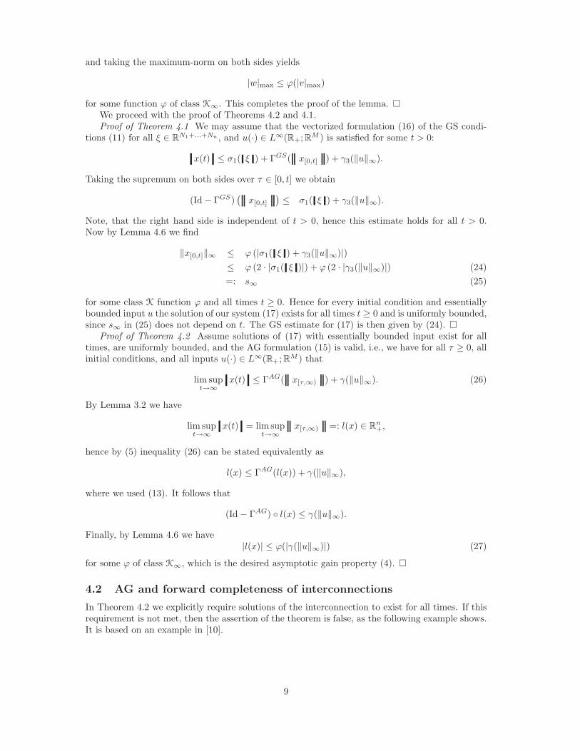
In Theorem 4.2 we explicitly require solutions of the interconnection to exist for all times. If thisrequirement is not met, then the assertion of the theorem is false, as the following example shows.It is based on an example in [10].

9

Example 4.7 Consider the planar autonomous system defined by

x = f(x, y) :=x2(y − x) + y5

(x2 + y2)(1 + (x2 + y2)2)(28)

y = g(x, y) :=y2(y − 2x)

(x2 + y2)(1 + (x2 + y2)2). (29)

It is shown in [10, §40, pp 191–194] that for (28) and (29) the origin is globally attracting butunstable.

Now replace (29) by

y = g(x, y, v) :=y2(y − 2x)

(x2 + y2)(1 + (x2 + y2)2)exp(v2), (30)

to obtain the system(

x

y

)

=

(f(x, y)

g(x, y, v)

)

, (31)

where v ∈ R is a parameter.By the same methods as in [10, §40, pp 191–194] it can be shown that for any fixed v ∈ R the

origin for system (31) is unstable, yet globally attracting. By symmetry it suffices to consider theopen upper half plane in R2. The proof is exactly as in [10] and therefore omitted.

Next we show, that for u(·) ∈ L∞(R+; R), ‖u‖∞ < m, the origin of the system(

x

y

)

=

(f(x, y)

g(x, y, u)

)

(32)

is globally attracting and unstable: Suppose a trajectory ϕ(·, (x0, y0)T , u(·)) of (32) starts in

(x0, y0)T lying in

Ψ+ := (x, y)T ∈ R2 : (x ≤ 0 and y > 0) or (x > 0 and y > 2x) .

In the region Ψ+ the second component of the trajectoryϕ(·) := ϕ(·, (x0, y0)

T , u(·)) is bounded by the second component of the trajectory η(·) := η(·, (x0, y0)T , ||u||∞)

of system (31) in the sense that for all t, τ ≥ 0 such that ϕ(t), η(τ) ∈ Ψ+ we have

ϕ(t)1 = η(τ)1 ⇒ ϕ(t)2 ≤ η(τ)2 .

This follows as for almost all t we have g(x, y, u(t)) ≤ g(x, y, ‖u‖∞).Now η(·) is known to reach the half line H := (x, y)T ∈ R2 : x ≥ 0, y = 2x in finite time

(using the argument provided in [10]). Since in Ψ+ we have x > 0 and y > 0, the trajectoryϕ(·, (x0, y0)

T , u) also hits the line H in finite time τ > 0 at the point (xτ , yτ )T .Define the “attracting set” A := (x, y)T ∈ R2 : y ≥ 0, x > 1

2y. Trajectories with bounded

input starting on the line H ⊂ A are ultimately attracted to the origin: On H every velocity vectorpoints into A, in A the y-component of each velocity vector is strictly negative. At some pointeach trajectory in A reaches a neighborhood of the x-axis, where all velocity vectors point to thelower left.

The preceding argument shows, that system (32) has the asymptotic gain property, with ar-bitrary small gain γ. So with slight abuse of notation we may choose γ = 0 as the asymptoticgain.

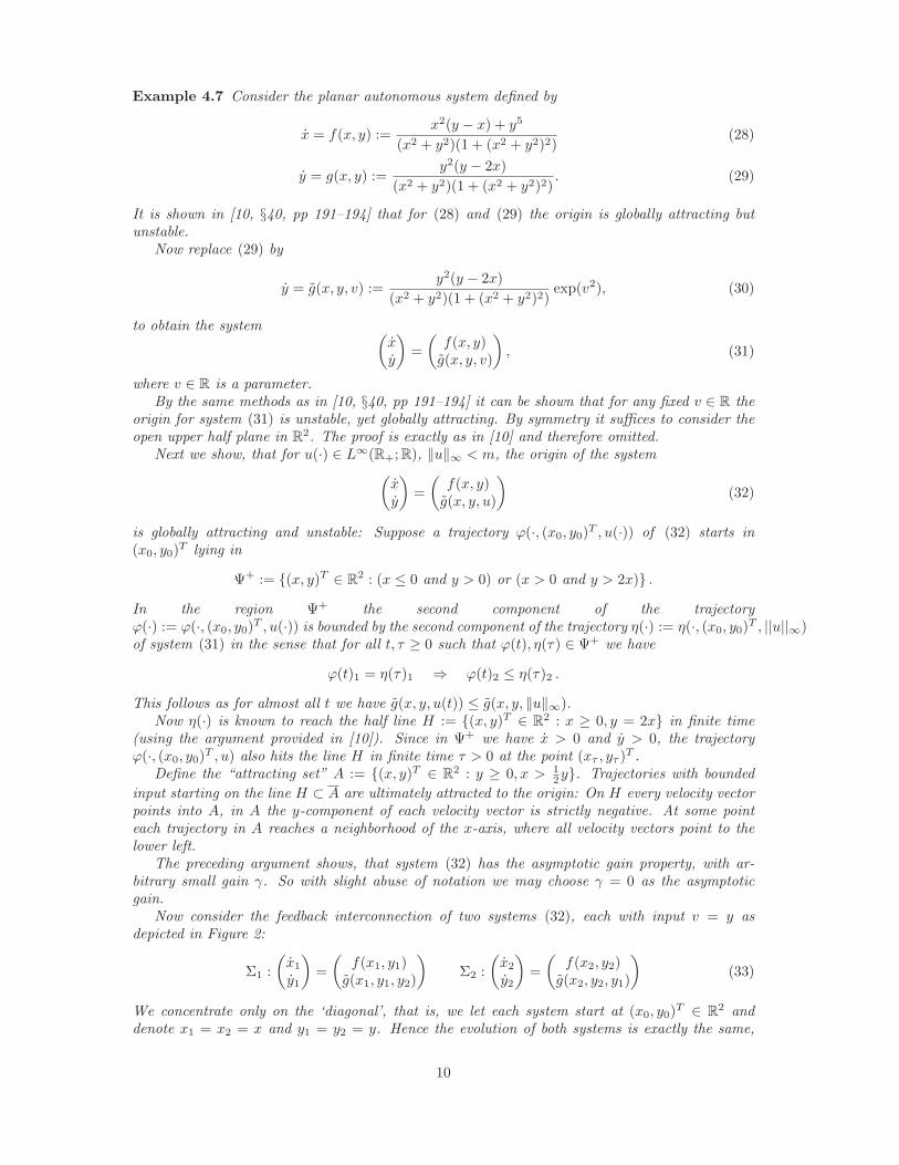
Now consider the feedback interconnection of two systems (32), each with input v = y asdepicted in Figure 2:

Σ1 :

(x1

y1

)

=

(f(x1, y1)

g(x1, y1, y2)

)

Σ2 :

(x2

y2

)

=

(f(x2, y2)

g(x2, y2, y1)

)

(33)

We concentrate only on the ‘diagonal’, that is, we let each system start at (x0, y0)T ∈ R2 and

denote x1 = x2 = x and y1 = y2 = y. Hence the evolution of both systems is exactly the same,

10

x1

v2 = y1

x2

v1 = y2

Σ1

Σ2

Figure 1: Feedback system (33).

motivating the term diagonal. The small gain condition, which in this case reduces to γ2 ≡ 0 < id,is clearly satisfied.

On the diagonal the dynamics are given by

x = f(x, y) , y = g(x, y, y) . (34)

For suitable initial conditions system (34) has a finite escape time, as the next calculation shows:Let V (x, y) = 1

2y2 be a Lyapunov function. We will show that V > V 2 along trajectories forsuitable initial conditions. This implies that not all trajectories of the feedback system exist for alltimes.

First we define the set Q :=

(x, y)T ∈ R2 : y > 0, 0 ≤ x <y(ey−y2−1)

2(ey−1)

. On Q we have

x <1

2y (35)

for system (33). Asymptotically we have y(ey−y2−1)2(ey−1) ≈ 1

2y as y → ∞. Also y(ey−y2−1)2(ey−1) < 1

2y for

all y > 0.Now we show that in the feedback system (33) a trajectory starting in (x, y) ∈ Q, with y > 6,

will always stay in Q (as long as it exists): To this end consider the horizontal distance between

ϕ(·, (x0, y0)T ) and the point

(12ϕ(t, (x0, y0)

T )2ϕ(t, (x0, y0)

T )2

)

on the half line H. This distance is just

d(t) =1

2ϕ(t, (x0, y0)

T )2 − ϕ(t, (x0, y0)T )1.

By (35) the derivative of d(t) satisfies

d(t) =1

2g(x, y, y) − f(x, y) > 0, (36)

for (x, y)T ∈ Q. Hence d(t) is non decreasing on the set Q. By (28) and (30) we have x > 0 andy > 0 on Q. Moreover, the right hand side boundary of Q approaches H, i.e., the distance betweenthis boundary and H decays monotonically for increasing values of y > 6. Hence the solutionϕ(·, (x0, y0)

T ) for (x0, y0)T ∈ Q must stay in Q, as long as it exists.

Now assume (x, y)T ∈ Q with y ≫ 1 sufficiently large and such that y > 2x + 1. By (36) iffollows that ϕ2(t) > 2ϕ1(t) + 1 for all t ≥ 0 along the trajectory ϕ with initial condition (x, y).Because of the dominating exponential term we have

V (x, y)[f(x, y) g(x, y, y)]T =y3(y − 2x) exp(y2)

(x2 + y2)(1 + (x2 + y2)2)>

y3 exp(y2)

(x2 + y2)(1 + (x2 + y2)2)>

1

4y4 = (V (x, y))2

along trajectories, provided that y is sufficiently large. Finally, V > V 2 implies a finite escapetime for the y-component.

Concluding, this example shows that although systems have the asymptotic gain property and thesmall gain condition is satisfied, Theorem 4.2 may not be applicable to the feedback interconnection,since solutions of the interconnected system do not exist for all times.

11

0 2 4 6 8 10 120

1

2

3

4

5

6

7

8

9

10

x

y

Q A

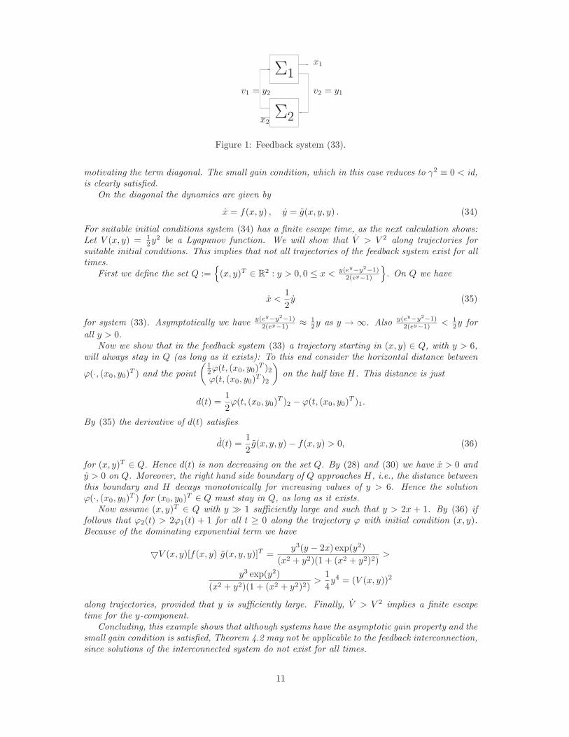
Figure 2: A trajectory of the (30) in Example 2: The dashed trajectory starts in (−1, 1)T withinput

√3 sin(t). The solid trajectory starts in the same point with constant input equal to

√3.

The half line H with (slope 2) is dashed dotted. The regions Q and A are depicted as well.

12

4.3 The maximum formulation of ISS

The ISS estimates for (8) can be formulated equivalently using the maximum instead of a sum-mation. Using the maximum the condition for ISS is

‖ϕi(t, ξ0i , xj , j 6= i, u)‖ ≤ max

jβ(‖ξ0

i ‖, t), γij(‖xj‖∞), γu(‖u‖∞), (37)

for i = 1, . . . , n, all initial conditions and all measurable bounded inputs. Note that to obtain suchan estimate for a particular system the gains γij , γu are in general different from the gains thatwould be used in an ISS inequality using summation as in (9). Still we can write down the gainmatrix Γ = ΓISS as we did before and define the max-operator Γ⊗ by

Γ⊗(s)i := maxj

γij(sj). (38)

If the gains γij are all linear, then Γ⊗ is a max linear operator [19]. Note that this is not the sameas a max-plus linear operator.

In the discrete time context Teel [29] proves that if we have maximum ISS estimates of thetype (37) for each subsystem and if for each cycle (or equivalently, each minimal cycle) in Γ wehave

γk1k2 γk2k3

. . . γkp−1kp< id,

for all (k1, . . . , kp) ∈ 1, . . . , np where k1 = kp, then the network under consideration is input-to-state stable. This result extends in a straightforward manner to continuous time systems. It is aneasy exercise to show that the cycle condition and the statement

Γ⊗(s) s, ∀s ∈ Rn+, s 6= 0,

are equivalent. Note that this relies crucially on the operation defined in (38) and does not holdfor the operator Γ defined earlier.

In [21] Potrykus et al. prove a similar but rather involved small gain theorem for continuoustime systems; their small gain condition is not at first sight equivalent to the one in [29].

For real non negative matrices it is known that the linear cycle condition and that the maxspectral radius is less than unity are equivalent, a nice survey on this topic can be found in Lur [19].In general µ(A) ≤ ρ(A), where µ(A) is the maximal cycle geometric mean of a non negative matrixA (corresponding to the cycle condition), and ρ(A) is the usual spectral radius of A, c.f. [19].

Now given a gain matrix Γ = (γij)ni,j=1 we associate two operators Rn

+ → Rn+, namely the

one given by Γ(s)i =∑

j γij(sj) and the one given by Γ⊗(s)i = maxj γij(sj), where s ∈ Rn+,

i = 1, . . . , n. The small gain conditionΓ id (39)

is a stronger condition on the gains than

Γ⊗ id, (40)

both are sufficient conditions for the max-formulation of the ISS small gain theorem for networks,but the latter is not sufficient for the sum-formulation. For the case n = 2 with γ11 = γ22 = 0,both conditions are equivalent, but for n ≥ 3 condition (39) is strictly stronger than condition (40),as can be shown easily by a linear example.

4.4 Discrete time systems

We now briefly discuss the extension of our result to the discrete time setting. In [15] Jiang et al.prove an ISS small gain theorem for discrete time systems, while in [12] they derive a small gaintheorem for locally input-to-state stable systems. Both papers use the maximum formulation ofISS.

In [17] Laila and Nesic consider parameterized discrete time systems that are semi globallypractically ISS and give a small gain theorem for two such systems in feedback interconnection.

13

Input-to-state stability for discrete time systems is defined in analogy to the continuous timecase, but with time R+ replaced by N = 0, 1, 2, . . .:

In this subsection we denote by [0, k] the set 0, . . . , k and by ‖x‖∞ = supl∈Nxl for functionsx : N → RN .

Consider the interconnected discrete time system

Σ :

Σ1 : x1(k + 1) = f1(x1(k), . . . , xn(k), u(k))...

Σn : xn(k + 1) = fn(x1(k), . . . , xn(k), u(k))

for k ∈ N, (41)

where xi(k) ∈ RNi , u(k) ∈ RM , and fi : RPn

j=1Nj+M → RNi is continuous.

System Σi is ISS, if there exits β ∈ KL and γij , γ ∈ K ∪ 0 with γii = 0, such that everysolution xi : N → RNi of (41) satisfies

|xi(k)| ≤ βi(|xi(0)|, k) +n∑

j=1

γij(||xj [0,k]||∞) + γ(||u||∞) (42)

for all inputs xj : N → RNj , j = 1, . . . , n, j 6= i, and u : N → RM .As a corollary of Theorem 4.4 we easily obtain the next result:

Proposition 4.8 Consider the systems Σi in (41) and suppose that each subsystem is ISS, i.e.,condition (42) holds for all i = 1, . . . , n. Let Γ = (γij)

ni,j=1. If there exists a mapping D as in

(19), such that(Γ D)(s) 6≥ s, ∀s ∈ Rn

+ \ 0 ,

then the system Σ in (41) is ISS from u to x.

Proof The assertion of Theorem 4.4 still is true if we replace system (8) by the discrete timesystem (41) and the definition of ISS by (42). Note that the proofs of Theorems 4.2, 4.1, and 4.4do not depend on the time set being a continuum or discrete set.

4.5 Linear gains

Suppose the gain functions γij are all linear, hence Γ is a linear mapping and (12) is just matrix-vector multiplication. In this case the network small gain condition (20) has a straightforwardinterpretation in terms of well known properties of matrices. The spectral radius of a matrix M

is denoted by ρ(M). For non-negative matrices Γ it is well known (see, e.g., [3, Theorem 2.1.1, p.26, and Theorem 2.1.11, p. 28]) that

(i) ρ(Γ) is an eigenvalue of Γ with a corresponding non-negative eigenvector,

(ii) if αx ≤ Γx holds for some x ∈ Rn+ \ 0 then α ≤ ρ(Γ).

Using this it is easy to see that for a non-negative matrix Γ ∈ Rn×n the following are equivalent:

(i) ρ(Γ) < 1,

(ii) ∀s ∈ Rn+ \ 0 : Γs 6≥ s,

(iii) Γk → 0, for k → ∞,

(iv) there exist a1, . . . , an > 0 such that ∀s ∈ Rn+ \ 0:

Γ(I + diag(a1, . . . , an))s 6≥ s.

Note that (iv) is the linear version of (20). As condition (i) makes no sense in the nonlinearsetting, (20) has been used as an extension to the nonlinear case. As a consequence we obtain

14

Corollary 4.9 Consider n interconnected ISS systems as in the previous section on the problemdescription with a linear gain matrix Γ, such that for the spectral radius ρ of Γ we have

ρ(Γ) < 1. (43)

Then the system defined by (17) is ISS from u to x.

Remark 4.10 For the case of large-scale interconnected input-output systems a result similar toCorollary 4.9 exists, cf. [32, p. 110]. It also covers Corollary 4.9 as a special case. The conditionon the spectral radius is quite the same and is applied to a matrix, whose entries are finite gainsof products of interconnection operators and corresponding subsystem operators. These gains arenon-negative numbers and, roughly speaking, defined as the minimal possible slope of affine boundson the interconnection operators.

5 Interpretation of the generalized small gain condition

In this section we wish to provide insight into the small gain condition of Theorem 4.4. We areconsidering Γ ∈ (K ∪ 0)n×n with zero diagonal as introduced in (12). The small gain conditionsufficient for ISS of an interconnection defined with maximum formulation is

Γ id , (44)

whereas for the robust condition, we need that there exists a diagonal D as in (19) such that

Γ D id , (45)

in case of ISS defined via summation.We first show, that Theorem 4.4 covers the known interconnection results for cascades and

feedback interconnections and discuss implications for the case of linear systems.Further, we investigate topological consequences of the small gain condition. Note that this

condition has an interesting interpretation for the stability analysis of a discrete time dynamicalsystem defined through the gain matrix Γ. Finally, an overview of all the interrelations is presented.

5.1 Connections to known results

As an easy consequence of Theorem 4.4 we recover, that an arbitrary feed forward cascade of ISSsubsystems is again ISS. If the subsystems are enumerated consecutively and the gain functionfrom subsystem j to subsystem i > j is denoted by γij , then the resulting gain matrix has non-zeroentries only below the diagonal. For arbitrary α ∈ K∞ the gain matrix with entries γij (IdR+

+α)for i > j and 0 for i ≤ j clearly satisfies (20). Therefore any feed forward cascade of ISS systemsis ISS.

Consider n = 2 in equation (8), i.e., two subsystems with linear gains. Then in Corollary 4.9we have

Γ =

[0 γ12

γ21 0

]

, γij ∈ R+

and ρ(Γ) < 1 if and only if γ12γ21 < 1. Hence we obtain the known small gain theorem, cf. [13]and [9].

For nonlinear gains and n = 2 the condition (20) in Theorem 4.4 reads as follows: There existα1, α2 ∈ K∞ such that

Γ D(s) =

(γ12 (Id + α2)(s2)γ21 (Id + α1)(s1)

)

(

s1

s2

)

,

for all s = (s1, s2)T ∈ R2

+. This is easily seen to be equivalent to

γ12 (Id + α2) γ21 (Id + α1)(t) < t , ∀t > 0. (46)

15

To this end we consider the vector [γ12 (Id + α2)(t), t]T for any t > 0. Applying Γ D we see

that the first component does not change, hence the second one must be less than t, which is just(46). The converse implication is obvious. Now inequality (46) is equivalent to the condition inthe small gain theorem of [14], namely, that for some α1, α2 ∈ K∞ it should hold that

(Id + α1) γ21 (Id + α2) γ12(s) ≤ s , ∀s > 0 , (47)

for all s ∈ R+, hence our theorem contains this result as a particular case.

Example 5.1 The condition (47) of [14] seems to be very similar to the small gain conditionγ12 γ21(s) < s of [13] and [9], however in these papers the maximum formulation of ISS is used,so that the interpretation of the gains is different. This similarity raises the question, whether thecompositions with (Id + αi), i = 1, 2 in (47) or more generally with D in (20) is necessary in thecontext of the summation formulation of ISS. The following example shows that this is indeed thecase.

Consider the equation

x = −x + u(1 − e−u), x(0) = x0 ∈ R, u ∈ R.

Integrating it follows

x(t) = e−tx0 +

∫ t

0

e−(t−τ)u(τ)(1 − e−u(τ)) dτ

≤ e−tx0 + ||u||∞(1 − e−||u||∞) = e−tx0 + γ(‖u‖∞),

with γ(s) = s(1 − e−s). Clearly γ(s) < s. Then for a feedback system

x1 = −x1 + x2(1 − e−x2) + u(t), (48)

x2 = −x2 + x1(1 − e−x1) + u(t) (49)

we have ISS for each subsystem with xi(t) ≤ e−tx0i + γi(||xi||∞) + ηi(||u||∞), where γi(s) < s and

hence γ1 γ2(s) < s for s > 0, but there are solutions x1 = x2 = const given by

x1 = −x2e−x2 + u, with u = x2e

−x2 .

Here x1 = x2 can be chosen arbitrary large with u → 0 for x1 → ∞, so that the system cannotsatisfy the asymptotic gain property and is therefore not ISS. Hence the condition Γ(s) s, forall s ∈ Rn

+ \ 0, or for two subsystems γ12 γ21(s) < s, for all s > 0, is not sufficient for theinput-to-state stability of the composite system in the nonlinear case.

Application to linear systems Linear systems are an important special case for which theresults are applicable. Consider the following setup where in the sequel we omit the external inputfor notational simplicity. Let

xj = Ajxj , xj ∈ RNj , j = 1, . . . , n (50)

describe n globally asymptotically stable linear systems, which are interconnected through

xj = Ajxj +n∑

k=1

∆jkxk j = 1, . . . , n, (51)

which can be rewritten asx = (A + ∆)x, (52)

where A is block diagonal, A = diag(Aj , j = 1, . . . , n), each Aj is Hurwitz and the matrix ∆ =(∆jk) is also in block form and encodes the connections between the n subsystems. We supposethat ∆jj = 0 for all j. Define the matrix R = (rjk), R ∈ Rn×n

+ , by rjk := ||∆jk||. For eachsubsystem, there exist positive constants Mj , λj , such that ‖eAjt‖ ≤ Mje

−λjt for all t ≥ 0.

Define a matrix D ∈ Rn×n+ by D := diag(

Mj

λj, j = 1, . . . , n). It is easy to see that in this case

the gain matrix ΓISS = DR. Then from Corollary 4.9 we obtain

16

Corollary 5.2 If ρ(D · R) < 1 then (52) is globally asymptotically stable.

Note that this is a special case of a theorem, which can be found in Vidyasagar [32, p. 110], seeRemark 4.10. The corollary is also a consequence of more general and precise results of a recentpaper [16] by Hinrichsen, Karow and Pritchard.

5.2 Topological consequences of the small gain condition

For the following statement we define the open domains

Ωi =

s ∈ Rn

+ : si >∑

j 6=i

γij(sj)

, i = 1, . . . , n.

Note that Ωi = s ∈ Rn+ : si > Γ(s)i. Also we need the simplex ∆r defined as the intersection of

the positive orthant Rn+ with the hyperplane s1 + · · · + sn = r > 0. The vertices of ∆r are given

by re1, . . . , ren (where ei denotes the i-th unit vector). The convex hull is denoted of a set C isdenoted by conv (C).

Proposition 5.3 Consider Γ ∈ (K∪0)n×n with zero diagonal. Then condition (44) is equivalentto

⋃ni=1 Ωi = Rn

+ \ 0. Furthermore (44) implies that for all r > 0

∆r ∩n⋂

i=1

Ωi 6= ∅. (53)

Proof Let s 6= 0. Formula (44) is equivalent to the existence of at least one index i ∈ 1, . . . , nwith si >

∑

j 6=i γij(sj). This proves the first part of the assertion.To prove the second part we will use the Knaster-Kuratovski-Mazurkiewicz (KKM) theorem

(see [11]), a topological fixed point theorem for simplices. The KKM theorem states that if forany face of ∆r given by σ(rei1 , . . . , reik

) = conv rei1 , . . . , reik, k ∈ 1, . . . , n, 1 ≤ i1 < i2 <

. . . < ik ≤ n we haveσ(rei1 , . . . , reik

) ⊂ ∪kj=1Ωij

,

then (53) follows.Without loss of generality consider a face σ = conv re1, . . . , rek (the other cases follow by

permutation) and let s ∈ σ. By assumption Γ(s) s, so there is an index i such that Γ(s)i < si.As Γ(s) ≥ 0 it follows that for this index si > 0. Hence 1 ≤ i ≤ k. This shows s ∈ Ωi for some1 ≤ i ≤ k and the assumptions of the KKM theorem are satisfied. This completes the proof.

We need the following invariance property of ∩iΩi.

Lemma 5.4 Consider Γ ∈ (K∪0)n×n with zero diagonal and assume (44). Assume that Γ hasno zero row. If s > 0 satisfies s ∈ ∩iΩi, then Γ(s) ∈ ∩iΩi.

Proof First note, that as s > 0 and as Γ has no zero rows, it follows that Γ(s) > 0. Furthermore,s ∈ ∩iΩi is equivalent to Γ(s) < s. Applying Γ to this inequality it follows from monotonicity ofΓ that Γ2(s) < Γ(s), which is equivalent to Γ(s) ∈ ∩iΩi.

Note in particular that the set⋂n

i=1 Ωi is unbounded. It is of further interest to know, that itis unbounded in all components. This will provide the key argument in the stability analysis ofthe associated discrete time system s(k + 1) = Γ(s(k)). However, this is not true in general. Wetherefore note

Proposition 5.5 Consider Γ ∈ (K∞ ∪ 0)n×n with zero diagonal and assume (44). If Γ isirreducible, then for any s ∈ Rn

+ there is a z ∈ ∩iΩi such that z ≥ s.

17

Proof We first assume that Γ is primitive. Let k0 be the non-negative integer given byLemma A.1a), such that Pi Γk0 Rj ∈ K∞ for any i, j, where P denotes a projection,R an injection. See Section 2 for the definitions of P and R. Fix s ≥ 0. For t ∈ [0,∞), i = 1, . . . , nwe define

Γk0

i (t) := Γk0 Ri(t) .

As Pi Γk0 Rj ∈ K∞ for all i, j = 1, . . . , n, there is a T ∈ R+ such that for all i = 1, . . . , nwe have

Γk0

i (t) > s for all t ≥ T. (54)

Choose r = nT and v > 0, v ∈ ∆r ∩ (∩iΩi). Such a v exists as the intersection ∩iΩi is open in∆r. Then vi ≥ T for some 1 ≤ i ≤ n and so

Γk0(v) ≥ maxj

Γk0

j (vj) ≥ Γk0

i (vi) ≥ Γk0

i (T ) > s .

By Lemma 5.4 we have Γk0(v) ∈ ∩iΩi. This completes the proof for the case that Γ is primitive.In the case that Γ is not primitive we apply Lemma A.1b). So without loss of generality, we

have a block-diagonal power Γν of Γ, where each of the square blocks on the diagonal is primitive.Then arguing as before, for every s we can choose a v > 0, v ∈ ∩iΩi so that

Γk0ν(v) > s .

This completes the proof.

Ω3

Ω2

Ω1

Figure 3: Overlapping of Ωi domains in R3

Let us briefly explain a further reason, why the overlapping condition (53) is interesting, apartfrom the fact, that Proposition 5.5 is important for the results of the next section. From thetheory of ISS-Lyapunov functions (see, e.g., [13]) it is known, that a system of the form (3) isISS if and only if it has a smooth ISS-Lyapunov function. In the context of n interconnectedsystems the small gain condition states, according to Proposition 5.3, that along trajectories ofthe interconnection

(i) in every state there is one subsystem with a decaying Lyapunov function,

18

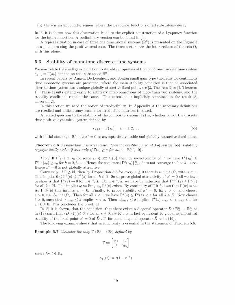
(ii) there is an unbounded region, where the Lyapunov functions of all subsystems decay.

In [6] it is shown how this observation leads to the explicit construction of a Lyapunov functionfor the interconnection. A preliminary version can be found in [4].

A typical situation in case of three one dimensional systems (R3) is presented on the Figure 3on a plane crossing the positive semi axis. The three sectors are the intersections of the sets Ωi

with this plane.

5.3 Stability of monotone discrete time systems

We now relate the small gain condition to stability properties of the monotone discrete time systemsk+1 = Γ(sk) defined on the state space Rn

+.In recent papers by Angeli, De Leenheer, and Sontag small gain type theorems for continuous

time monotone systems are presented, where the main stability condition is that an associateddiscrete time system has a unique globally attractive fixed point, see [2, Theorem 3] or [1, Theorem1]. These results extend easily to arbitrary interconnections of more than two systems, and thestability conditions remain the same. This extension is implicitly contained in the result [8,Theorem 2].

In this section we need the notion of irreducibility. In Appendix A the necessary definitionsare recalled and a dichotomy lemma for irreducible matrices is stated.

A related question to the stability of the composite system (17) is, whether or not the discretetime positive dynamical system defined by

sk+1 = Γ(sk), k = 1, 2, . . . (55)

with initial state s0 ∈ Rn+ has x∗ = 0 as asymptotically stable and globally attractive fixed point.

Theorem 5.6 Assume that Γ is irreducible. Then the equilibrium point 0 of system (55) is globallyasymptotically stable if and only if Γ(s) s for all s ∈ Rn

+ \ 0.

Proof If Γ(s0) ≥ s0 for some s0 ∈ Rn+ \ 0 then by monotonicity of Γ we have Γk(s0) ≥

Γk−1(s0) ≥ s0 for k = 2, 3, . . .. Hence the sequence Γk(s0)∞k=0 does not converge to 0 as k → ∞.Hence x∗ = 0 is not globally attractive.

Conversely, if Γ id, then by Proposition 5.5 for every s ≥ 0 there is a z ∈ ∩iΩi with s < z.This implies 0 ≤ Γk(s) ≤ Γk(z) for all k ∈ N. So to prove global attractivity of x∗ = 0 all we haveto show is that Γk(z) → 0 for z ∈ ∩iΩi. For z ∈ ∩iΩi we have by induction that Γk+1(z) ≤ Γk(z)for all k ∈ N. This implies w := limk→∞ Γk(z) exists. By continuity of Γ it follows that Γ(w) = w.As Γ id this implies w = 0. Finally, to prove stability of x∗ = 0, fix ε > 0, and choosez > 0, z ∈ ∆ε ∩ ∩iΩi. Then for all s < z we have Γk(s) ≤ Γk(z) < z for all k ∈ N. Now chooseδ > 0, such that |s|max ≤ δ implies s < z. Then |s|max ≤ δ implies |Γk(s)|max < |z|max < ε forall k ≥ 0. This concludes the proof.

In [5] it is shown, that the condition, that there exists a diagonal operator D : Rn+ → Rn

+ asin (19) such that (D Γ)(s) s for all s 6= 0, s ∈ Rn

+, is in fact equivalent to global asymptotical

stability of the fixed point x∗ = 0 of D Γ, for some diagonal operator D as in (19).The following example shows that irreducibility is essential in the statement of Theorem 5.6.

Example 5.7 Consider the map Γ : R2+ → R2

+ defined by

Γ :=

[γ11 id0 γ22

]

where for t ∈ R+

γ11(t) := t(1 − e−t)

19

and the function γ22 is constructed in the sequel. First note that γ11 ∈ K∞ and γ11(t) < t, ∀t > 0.Let εk∞k=1 be a strictly decreasing sequence of positive real numbers, such that limk→∞ εk = 0

and limK→∞

∑Kk=1 εk = ∞. For k = 1, 2, . . . define

γ22

(

εk + (1 +

k−1∑

j=1

εj)e−(1+

Pk−1

j=1εj)

)

:= εk+1 + (1 +

k∑

j=1

εj)e−(1+

Pkj=1

εj)

and observe that

εk + (1 +

k−1∑

j=1

εj)e−(1+

Pk−1

j=1εj) > εk+1 + (1 +

k∑

j=1

εj)e−(1+

Pkj=1

εj) ,

since εk > εk+1 for all k = 1, 2, . . . and the map t 7→ t · e−t is strictly decreasing on (1,∞).Moreover we have by assumption, that

εk + (1 +

k−1∑

j=1

εj)e−(1+

Pk−1

j=1εj) −−−−→

k→∞0.

These facts together imply that γ22 may be extrapolated to some K∞-function, in a way suchthat γ22(t) < t, ∀t > 0 holds.

Note that by our particular construction we have Γ(s) s for all s ∈ R2+ \ 0. Now define

s1 ∈ R2+ by

s1 :=

[1

1 + e−1

]

and for k = 1, 2, . . . recursively define sk+1 := Γ(sk) ∈ R2+.

By induction one verifies that

sk+1 = Γk(s1) =

[

1 +∑k

j=1 εj

εk+1 + (1 +∑k

j=1 εj)e−(1+

Pkj=1

εj)

]

.

By our previous considerations and assumptions we easily obtain that the second componentof the sequence sk∞k=1 strictly decreases and converges to zero as k tends to infinity. But at thesame time the first component strictly increases above any given bound.

Hence we established that Γ(s) s ∀s 6= 0 in general does not imply ∀s 6= 0 : Γk(s) → 0 ask → ∞. For this example it is also easy to verify that ∩iΩi is not unbounded in all components.So that the assertion of Proposition 5.5 is false in this case.

Remark 5.8 Note that we can even turn the constructed 2x2-Γ into the null-diagonal form toconform with the structure of gain matrices in Section 3. Using the same notation for γij as inExample 5.7, we just define

Γ :=

0 γ11 id 0γ11 0 0 id0 0 0 γ22

0 0 γ22 0

and s1 :=

11

1 + e−1

1 + e−1

and easily verify that Γk(s1) does not converge to 0.

5.4 Summary map of the interpretations concerning Γ

In Figure 4 we summarize the relations between various statements about Γ that were proved inSection 5.

20

∃D as in (19) : Γ D(s) s

⇓ (⇑ if Γ is linear)

s(k + 1) = Γ(s(k))is 0-GAS

⇒⇐∗

Γ(s) s ⇐⇒

n⋃

i=1

Ωi = RN \ 0

∀r > 0 :

n⋂

i=1

Ωi ∩ ∆r 6= ∅

m if Γ is linear

ρ(Γ) < 1

Figure 4: Some implications and equivalences of the generalized small gain condition. All state-ments are supposed to hold for all s ∈ Rn

+, s 6= 0. The implication denoted by ∗ holds if Γ is linearor irreducible.

6 Conclusions

We considered a composite system consisting of an arbitrary number of nonlinear arbitrarilyinterconnected input-to-state stable subsystems, as they arise in applications.

For this general case a network version of the nonlinear small gain theorem has been obtained.For linear interconnection gains this is a special case of a known result, cf. [32, page 110]. Ithas been shown how the generalized small gain theorem can be applied to the analysis of linearsystems and further implications of the small gain condition have been discussed to clarify itssignificance. The problem of constructing Lyapunov functions within this framework will be dealtwith in [6].

Acknowledgements:We like to thank the anonymous reviewers for their useful remarks and comments on an earlier

version of this paper. This research is funded by the German Research Foundation (DFG) aspart of the Collaborative Research Center 637 ”Autonomous Cooperating Logistic Processes: AParadigm Shift and its Limitations” (SFB 637).

A Non-negative matrices and graphs

A (finite) directed graph G = V,E consists of a set of vertices V and a set of edges E ⊂ V × V .We may identify V = 1, . . . , n in case of n vertices. The adjacency matrix AG = (aij) of thisgraph is defined by

aij =

1 if (j, i) ∈ E,

0 else.

Conversely, given an n × n-matrix A, a graph G(A) = V,E is defined by V := 1, . . . , n andE = (j, i) ∈ V × V : aij 6= 0.

There are several concepts and results of (non-negative) matrix theory, which are of purelygraph theoretical nature. Hence the same can be done for our gain matrix Γ. We may associate agraph G(Γ), which represents the interconnections between the subsystems, in the same manner,as we would do for matrices.

The graph of a power Γk of Γ consists of the same set of vertices V as Γ and has edgesE = (j, i) ∈ V × V : Component j influences component i. This can be stated equivalently asE = (j, i) ∈ V × V : ∃s ∈ Rn

+ : t 7→ Pi Γk(s + t · ej) is of class K or E = (j, i) ∈ V × V :

21

∀s ∈ Rn+ : t 7→ Pi Γk(s + t · ej) is of class K. With this notation we have

A(Γk) = A(G((A(Γ))k)), (56)

where the right hand side denotes the adjacency matrix of the graph associated to the matrix(A(Γ))k, that is the graph with edges E = (i, j) ∈ V × V : (A(Γ))k)ij 6= 0.

We say Γ is irreducible, if G(Γ) is strongly connected, that is, for every pair of vertices (i, j)there exists a sequence of edges (a path) connecting vertex i to vertex j. Obviously Γ is irreducibleif and only if ΓT is. Γ is called reducible if it is not irreducible.

The gain matrix Γ is primitive, if there exists a positive integer m such that (AGΓ)m has only

positive entries.For the following facts only the graph structure associated to a gain matrix is relevant.If Γ is reducible, then a permutation transforms it into a block upper triangular matrix. From

an interconnection point of view, this splits the system into cascades of subsystems each withirreducible (or zero) adjacency matrix.

Lemma A.1 Assume the gain matrix Γ is irreducible. Then there are two distinct cases:

a) The gain matrix Γ = (γij(·)), where γij(·) ∈ K or γij = 0, is primitive and hence there is anon-negative integer k0 such that Γk0 fulfills Pi Γk0 Rj ∈ K for any i, j.

b) The gain matrix Γ can be transformed to

PΓPT =

0 Γ12 0 . . . 0

0 0 Γ23 . . . 0...

.... . .

...

0 0 0 . . . Γν−1,ν

Γν1 0 0 . . . 0

=: Γ (57)

using some permutation matrix P , where the zero blocks on the diagonal are square andwhere the adjacency matrix of Γν is of block diagonal form with square primitive blocks onthe diagonal. Here ν is the index of imprimitivity, which is the number of nonzero blocks inthe above definition of Γ.

Proof Let AGΓbe the adjacency matrix corresponding to the graph associated with Γ. This

matrix is primitive if and only if Γ is primitive. Note that the (i, j)th entry of AkGΓ

is zero if

and only if the (i, j)th entry of Γk is zero. Multiplication of Γ by a permutation matrix onlyrearranges the positions of the class K-functions, hence this operation is well defined. From theseconsiderations it is clear, that it is sufficient to prove the lemma for the matrix A := AGΓ

. Butfor non-negative matrices this result follows from standard results in the theory of non-negativematrices, see, e.g., [3] or [18].

References

[1] D. Angeli, P. De Leenheer, and E. D. Sontag. A small-gain theorem for almost global con-vergence of monotone systems. Systems Control Lett., 52(5):407–414, 2004.

[2] D. Angeli and E. Sontag. Interconnections of monotone systems with steady-state characteri-stics. In Optimal control, stabilization and nonsmooth analysis, volume 301 of Lecture Notesin Control and Inform. Sci., pages 135–154. Springer, Berlin, 2004.

[3] A. Berman and R. J. Plemmons. Nonnegative matrices in the mathematical sciences. Acade-mic Press [Harcourt Brace Jovanovich Publishers], New York, 1979.

22

[4] S. Dashkovskiy, B. S. Ruffer, and F. R. Wirth. Construction of ISS Lyapunov functions fornetworks. Technical Report 06-06, Zentrum fur Technomathematik, University of Bremen,Technical Report, Juli 2006.

[5] S. Dashkovskiy, B. S. Ruffer, and F. R. Wirth. Discrete time monotone systems: Criteriafor global asymptotic stability and applications. In Proceedings of the 17th InternationalSymposium on Mathematical Theory of Networks and Systems (MTNS), Kyoto, Japan, pages89–97, July 24-28 2006.

[6] S. Dashkovskiy, B. S. Ruffer, and F. R. Wirth. Explicit ISS Lyapunov functions for networks.In preparation, 2006.

[7] S. Dashkovskiy, B. S. Ruffer, and F. R. Wirth. An ISS Lyapunov function for networks ofISS systems. In Proceedings of the 17th International Symposium on Mathematical Theory ofNetworks and Systems (MTNS), Kyoto, Japan, pages 77–82, July 24-28 2006.

[8] G. A. Enciso and E. D. Sontag. Global attractivity, I/O monotone small-gain theorems, andbiological delay systems. Discrete Contin. Dyn. Syst., 14(3):549–578, 2006.

[9] L. Grune. Input-to-state dynamical stability and its Lyapunov function characterization.IEEE Trans. Automat. Control, 47(9):1499–1504, 2002.

[10] W. Hahn. Stability of motion. Springer-Verlag New York, Inc., New York, 1967.

[11] C. D. Horvath and M. Lassonde. Intersection of sets with n-connected unions. Proc. Am.Math. Soc., 125(4):1209–1214, 1997.

[12] Z.-P. Jiang, Y. Lin, and Y. Wang. Nonlinear small-gain theorems for discrete-time feedbacksystems and applications. Automatica J. IFAC, 40(12):2129–2136 (2005), 2004.

[13] Z.-P. Jiang, I. M. Y. Mareels, and Y. Wang. A Lyapunov formulation of the nonlinear small-gain theorem for interconnected ISS systems. Automatica J. IFAC, 32(8):1211–1215, 1996.

[14] Z.-P. Jiang, A. R. Teel, and L. Praly. Small-gain theorem for ISS systems and applications.Math. Control Signals Systems, 7(2):95–120, 1994.

[15] Z.-P. Jiang and Y. Wang. Input-to-state stability for discrete-time nonlinear systems. Auto-matica J. IFAC, 37(6):857–869, 2001.

[16] M. Karow, D. Hinrichsen, and A. J. Pritchard. Interconnected systems with uncertain coup-lings: Explicit formulae for mu-values, spectral value sets, and stability radii. SIAM J. ControlOptim., 45(3):856–884, 2006.

[17] D. S. Laila and D. Nesic. Discrete-time Lyapunov-based small-gain theorem for parameterizedinterconnected ISS systems. IEEE Trans. Automat. Control, 48(10):1783–1788, 2003.

[18] P. Lancaster and M. Tismenetsky. The theory of matrices. Academic Press Inc., Orlando,FL, second edition, 1985.

[19] Y.-Y. Lur. On the asymptotic stability of nonnegative matrices in max algebra. LinearAlgebra Appl., 407:149–161, 2005.

[20] A. N. Michel and R. K. Miller. Qualitative analysis of large scale dynamical systems. AcademicPress [Harcourt Brace Jovanovich Publishers], New York, 1977.

[21] H. G. Potrykus, F. Allgower, and S. J. Qin. The character of an idempotent-analytic nonlinearsmall gain theorem. In Positive systems (Rome, 2003), volume 294 of Lecture Notes in Controland Inform. Sci., pages 361–368. Springer, Berlin, 2003.

23

[22] N. Rouche, P. Habets, and M. Laloy. Stability theory by Liapunov’s direct method. Springer-Verlag, New York, 1977.

[23] D. D. Siljak. Large-scale dynamic systems, volume 3 of North-Holland Series in SystemScience and Engineering. North-Holland Publishing Co., New York, 1979.

[24] E. Sontag and A. Teel. Changing supply functions in input/state stable systems. IEEE Trans.Automat. Control, 40(8):1476–1478, 1995.

[25] E. D. Sontag. Smooth stabilization implies coprime factorization. IEEE Trans. Automat.Control, 34(4):435–443, 1989.

[26] E. D. Sontag. The ISS philosophy as a unifying framework for stability-like behavior. InNonlinear control in the year 2000, Vol. 2 (Paris), volume 259 of Lecture Notes in Controland Inform. Sci., pages 443–467. Springer, London, 2001.

[27] E. D. Sontag and Y. Wang. New characterizations of input-to-state stability. IEEE Trans.Automat. Control, 41(9):1283–1294, 1996.

[28] G. Szasz. Introduction to lattice theory. Third revised and enlarged edition. MS revised byR. Wiegandt; translated by B. Balkay and G. Toth. Academic Press, New York, 1963.

[29] A. R. Teel. Input-to-state stability and the nonlinear small gain theorem. Private communi-cation, 2005.

[30] A. R. Teel. A nonlinear small gain theorem for the analysis of control systems with saturation.IEEE Trans. Automat. Control, 41(9):1256–1270, 1996.

[31] A. R. Teel. Connections between Razumikhin-type theorems and the ISS nonlinear small gaintheorem. IEEE Trans. Automat. Control, 43(7):960–964, 1998.

[32] M. Vidyasagar. Input-output analysis of large-scale interconnected systems, volume 29 ofLecture Notes in Control and Information Sciences. Springer-Verlag, Berlin, 1981.

24