AN IRREGULARLY PORTIONED FDF SOLVER

FOR TURBULENT FLOW SIMULATION

by

Patrick H. Pisciuneri

Submitted to the Graduate Faculty of

the Swanson School of Engineering in partial fulfillment

of the requirements for the degree of

Doctor of Philosophy

University of Pittsburgh

2013

UNIVERSITY OF PITTSBURGH

SWANSON SCHOOL OF ENGINEERING

This dissertation was presented

by

Patrick H. Pisciuneri

It was defended on

July 16, 2013

and approved by

Peyman Givi, Ph.D., James T. MacLeod Professor of Mechanical Engineering and

Materials Science, Professor of Chemical and Petroleum Engineering

William S. Slaughter, Ph.D., Associate Professor of Mechanical Engineering and Materials

Science

Albert C. To, Ph.D., Assistant Professor of Mechanical Engineering and Materials Science

Nadine Aubry, Ph.D., Dean of the College of Engineering, Northeastern University

Dissertation Director: Peyman Givi, Ph.D., James T. MacLeod Professor of Mechanical

Engineering and Materials Science, Professor of Chemical and Petroleum Engineering

ii

Copyright c© by Patrick H. Pisciuneri

2013

iii

AN IRREGULARLY PORTIONED FDF SOLVER FOR TURBULENT FLOW

SIMULATION

Patrick H. Pisciuneri, PhD

University of Pittsburgh, 2013

A new computational methodology is developed for large eddy simulation (LES) with the

filtered density function (FDF) formulation of turbulent reacting flows. This methodology

is termed the “irregularly portioned Lagrangian Monte Carlo finite difference” (IPLMCFD).

It takes advantage of modern parallel platforms and mitigates the computational cost of

LES/FDF significantly. The embedded algorithm addresses the load balancing issue by

decomposing the computational domain into a series of irregularly shaped and sized subdo-

mains. The resulting algorithm scales to thousands of processors with an excellent efficiency.

Thus it is well suited for LES of reacting flows in large computational domains and under

complex chemical kinetics. The efficiency of the IPLMCFD; and the realizability, consistency

and the predictive capability of FDF are demonstrated by LES of several turbulent flames.

iv

TABLE OF CONTENTS

PREFACE . . . . . . . . . . . . . . . . . . . . . . . . . . . . . . . . . . . . . . . . . ix

1.0 INTRODUCTION . . . . . . . . . . . . . . . . . . . . . . . . . . . . . . . . . 1

1.1 SGS CLOSURE IN TURBULENT COMBUSTION . . . . . . . . . . . . . . 2

1.2 SGS CLOSURES IN NONPREMIXED FLAMES . . . . . . . . . . . . . . . 3

1.3 SGS CLOSURES IN PREMIXED FLAMES . . . . . . . . . . . . . . . . . . 6

1.4 OBJECTIVE AND SCOPE . . . . . . . . . . . . . . . . . . . . . . . . . . . 7

2.0 IRREGULARLY PORTIONED FDF SIMULATOR . . . . . . . . . . . . 9

2.1 GOVERNING EQUATIONS . . . . . . . . . . . . . . . . . . . . . . . . . . 9

2.2 SGS CLOSURE FOR HYDRODYNAMICS . . . . . . . . . . . . . . . . . . 11

2.3 SFMDF . . . . . . . . . . . . . . . . . . . . . . . . . . . . . . . . . . . . . . 12

2.4 FDF SIMULATION . . . . . . . . . . . . . . . . . . . . . . . . . . . . . . . 13

2.5 IPLMCFD . . . . . . . . . . . . . . . . . . . . . . . . . . . . . . . . . . . . 15

2.6 RESULTS . . . . . . . . . . . . . . . . . . . . . . . . . . . . . . . . . . . . . 18

2.6.1 Scalability . . . . . . . . . . . . . . . . . . . . . . . . . . . . . . . . . 18

2.6.2 Realizability . . . . . . . . . . . . . . . . . . . . . . . . . . . . . . . . 22

2.6.3 Consistency and Reliability . . . . . . . . . . . . . . . . . . . . . . . . 25

3.0 CONCLUSIONS . . . . . . . . . . . . . . . . . . . . . . . . . . . . . . . . . . 36

3.1 FURTHER APPLICATIONS . . . . . . . . . . . . . . . . . . . . . . . . . . 36

3.2 OTHER FDF CLOSURES . . . . . . . . . . . . . . . . . . . . . . . . . . . 37

3.3 DYNAMIC PARTITIONING . . . . . . . . . . . . . . . . . . . . . . . . . . 37

3.4 HYBRID PARALLELISM . . . . . . . . . . . . . . . . . . . . . . . . . . . . 38

BIBLIOGRAPHY . . . . . . . . . . . . . . . . . . . . . . . . . . . . . . . . . . . . 39

v

LIST OF TABLES

1 Sandia Flame D simulation model parameters. . . . . . . . . . . . . . . . . . 28

2 ARM reaction steps and species. . . . . . . . . . . . . . . . . . . . . . . . . . 28

3 Sandia Flame D simulation thermochemistry inlet boundary conditions. . . . 29

vi

LIST OF FIGURES

1 Typical three-dimensional section of the domain in the hybrid simulation. Solid

cubes denote FD points. Spheres denote MC particles. The dashed line repre-

sents the ensemble domain. . . . . . . . . . . . . . . . . . . . . . . . . . . . 14

2 (a) Subdomain boundaries and (b) walltime per timestep for each subdomain

for the uniform decomposition. . . . . . . . . . . . . . . . . . . . . . . . . . 16

3 Instantaneous CPU time in milliseconds spent performing particle integration. 16

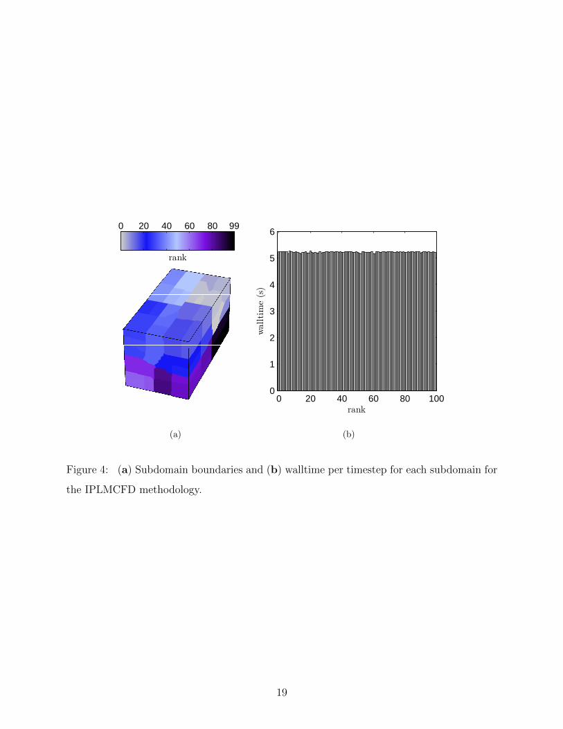
4 (a) Subdomain boundaries and (b) walltime per timestep for each subdomain

for the IPLMCFD methodology. . . . . . . . . . . . . . . . . . . . . . . . . . 19

5 (a) Strong scaling comparisons of the IPLMCFD vs. an unbalanced decompo-

sition. (b) Strong scaling of the IPLMCFD for an increasing number of MC

particles. . . . . . . . . . . . . . . . . . . . . . . . . . . . . . . . . . . . . . . 20

6 (a) Weak scaling comparisons of the IPLMCFD vs. an unbalanced decomposi-

tion for a fixed ratio of cells per processor. (b) Weak scaling of the IPLMCFD

for a fixed ratio of MC particles per processor. . . . . . . . . . . . . . . . . . 21

7 Performance in time of the IPLMCFD vs. an unbalanced decomposition. . . . 22

8 Scatter plots of the filtered composition variables vs. the filtered mixture

fraction for Da = 10−2 and Da = 102. The dashed lines denote pure mixing

and infinitely fast chemistry limits. . . . . . . . . . . . . . . . . . . . . . . . 23

9 Scatter plot comparing Z3 vs. the mixture fraction for Da = 102. . . . . . . 24

10 Sandia Flame D burner configuration. . . . . . . . . . . . . . . . . . . . . . 27

vii

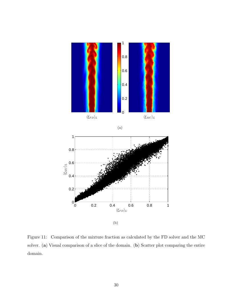
11 Comparison of the mixture fraction as calculated by the FD solver and the

MC solver. (a) Visual comparison of a slice of the domain. (b) Scatter plot

comparing the entire domain. . . . . . . . . . . . . . . . . . . . . . . . . . . 30

12 Isosurfaces of the mixture fraction, temperature and mass fraction of CO2. . 31

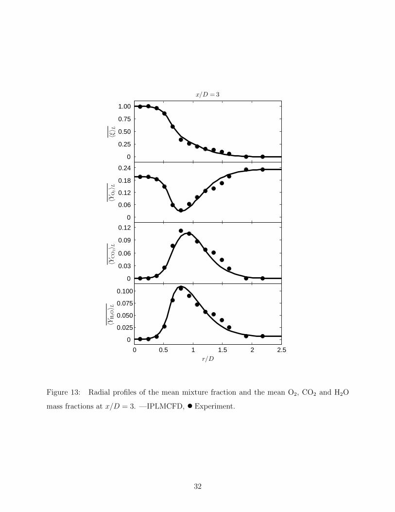
13 Radial profiles of the mean mixture fraction and the mean O2, CO2 and H2O

mass fractions at x/D = 3. —IPLMCFD, • Experiment. . . . . . . . . . . . 32

14 Radial profiles of the mean temperature and the mean CH4, CO and N2 mass

fractions at x/D = 3. —IPLMCFD, • Experiment. . . . . . . . . . . . . . . . 33

15 Radial profiles of the mean mixture fraction and the mean O2, CO2 and H2O

mass fractions at x/D = 7.5. —IPLMCFD, • Experiment. . . . . . . . . . . 34

16 Radial profiles of the mean temperature and the mean CH4, CO and N2 mass

fractions at x/D = 7.5. —IPLMCFD, • Experiment. . . . . . . . . . . . . . . 35

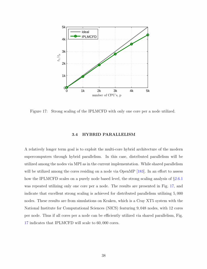
17 Strong scaling of the IPLMCFD with only one core per a node utilized. . . . 38

viii

PREFACE

Modeling of turbulent reacting flows requires knowledge in many areas including transport

phenomena, chemical kinetics and applied mathematics. Numerical simulation of such flows

requires knowledge of numerical methods, computational algorithms; and as I hope to con-

vince you in this work, parallel programming and high performance computing. Studying

such a broad range of subjects has been exciting and overwhelming; but also rewarding. The

fact that I made it this far is a testament to all the help that I received along the way.

I am sincerely grateful to my adviser, Professor Peyman Givi, for providing me this op-

portunity, and for his support, guidance and patience during my graduate studies. I would

like to thank the members of my doctoral committee, Professors Nadine Aubry, William

Slaughter and Albert To. Also, I would like to thank Professor Cyrus Madnia of the Univer-

sity at Buffalo. It has been a pleasure to collaborate and interact with his group. And I am

grateful to Dr. Peter Strakey and Dr. Nathan Weiland of the National Energy Technology

Laboratory, who have provided support and firsthand insight into many physical aspects of

turbulent combustion.

I would also like to thank all of my colleagues that I had the pleasure to work with

at one point or another during my time at the Laboratory for Computational Transport

Phenomena at the University of Pittsburgh: Dr. Naseem Ansari, Dr. Tomasz Drozda, Dr.

Mahdi Mohebbi, Dr. Mehdi Nik, Dr. Collin Otis, Mr. Sasan Salkhordeh, Dr. Reza Sheikhi

and Dr. Levent Yilmaz. I am particularly grateful to Drs. Nik, Sheikhi and Yilmaz, who

mentored me and showed me how to be successful as a new member of the group.

Most importantly, I would like to acknowledge my entire family, particularly my mom

& dad, my sister, Kellie, and my girlfriend, Noelle. They have provided love, support and

patience throughout this endeavor. I cannot thank them enough, only I hope that I have

grown into a better person during my time here at Pitt.

ix

As part of the National Energy Technology Laboratory’s Regional University Alliance

(NETL-RUA), a collaborative initiative of the NETL, this technical effort was performed

under the DOE-RES Contract DE-FE0004000. Additional support for this work is provided

by AFOSR & NASA under Grant FA9550-09-1-0611, by AFOSR under Grant FA9550-12-

1-0057, by NSF under Grant CBET-1250171, by the NSF Extreme Science and Engineering

Discovery Environment (XSEDE) under Grants TG-CTS070055N & TG-CTS120015; and

by the University of Pittsburgh Center for Simulation and Modeling.

PATRICK H. PISCIUNERI

UNIVERSITY OF PITTSBURGH, 2013

x

1.0 INTRODUCTION

The filtered density function (FDF) methodology [1] has proven to be very effective in the

subgrid scale (SGS) modeling required for large eddy simulation (LES) of turbulent reacting

flows. This methodology was first introduced by Givi [2] and then formally defined by Pope

[3]. It is basically the counterpart to the probability density function (PDF) approach used in

Reynolds averaged Navier-Stokes (RANS) simulations. The LES/FDF methodology is suited

for the treatment of large-scale, unsteady phenomena. Thus, when compared to RANS, it

provides a more detailed and reliable prediction of turbulent reacting flows [4].

The FDF has evolved extensively since its original conception. Colucci et al. [5] devel-

oped and solved the transport equation for the marginal scalar FDF (SFDF) suitable for

constant density flows. The variable density formulation of the SFDF was developed by

Jaberi et al. [6], and it is known as the scalar filtered mass density function (SFMDF).

The marginal velocity FDF (VFDF) was developed by Gicquel et al. [7]. Joint velocity-

scalar approaches have been developed for constant density (VSFDF) and variable density

(VSFMDF) flows by Sheikhi et al. [8, 9]. The current state of the art for LES of low-speed

flows is the frequency-velocity-scalar filtered mass density function (FVS-FMDF) and is due

to Sheikhi et al. [10]. The most systematic means of LES of high-speed flows is via the

energy-pressure-velocity-scalar filtered mass density function (EPVS-FMDF) and is due to

Nik [11, 12].

Despite its popularity, a major challenge still associated with the LES/FDF methodology

is its computational cost. This cost is exacerbated by the complexity of the chemical kinetics.

For moderately sized geometries with even reduced finite-rate kinetics simulations can take

on the order of a few years [13].

1

1.1 SGS CLOSURE IN TURBULENT COMBUSTION

The filtering operation in LES results in the subgrid scale (SGS) closure problem [2, 14].

This problem, particularly in regards to the chemical source term, has been the subject of

broad investigation, resulting in a variety of approaches [1, 15–20]. Typically, most models

are based on those which have shown success in RANS.

Combustion modes are often split into two categories [21]: nonpremixed and premixed.

It is helpful to differentiate between these two regimes as some of the models are for one

particular regime or the other. In nonpremixed combustion, the fuel and air streams are

introduced separately. Combustion occurs after the onset of mixing by molecular diffusion.

Thus, sometimes the label “diffusion flame” is adopted for this mode. Premixed flames

provide a mixture of fuel and oxidizer prior to entry into the combustor. They offer the

advantage of greater control over the reacting mixture. However, greater care is required in

the design of premixed combustors, as the mixture is volatile.

These two regimes are not entirely separate, as in most cases, the mode is via partially

premixed combustion. An example is a lifted flame. In such flames, fuel and air are separately

inserted into the combustor, as in the nonpremixed case. However, under suitable conditions

[22] if the flame is lifted from the burner, mixing of the fuel and air occurs before combustion,

as in the premixed case.

A survey of combustion literature reveals significant progress in LES of reacting turbulent

flows. It appears that Schumann [23] was one of the first to conduct LES of a reacting flow.

However, the assumption made in this work to simply neglect the contribution of SGS scalar

fluctuations to the filtered reaction rate is debatable. The importance of such fluctuations

has been long recognized in RANS in both combustion [24] and chemical engineering [25, 26].

To account for such fluctuations, significant progress has been made within the past 25 years.

In the next two sections, a review is made of some of the more widely used closures in both

combustion regimes.

2

1.2 SGS CLOSURES IN NONPREMIXED FLAMES

The obvious extension of Schumann’s method is to develop and solve transport equations

for the SGS higher order moments [27, 28]. These methods are not very powerful as the

number of moments to be considered does not converge. This is similar to the classical

closure problem in turbulence [29–31]. One remedy for this problem is to use PDF methods.

These methods go back to the pioneering work of Toor [32] and have been widely used in

RANS [2, 3, 33–37]. This approach offers the advantage that all the statistical information

pertaining to the scalar field is embedded within the PDF. Therefore, once the PDF is known

the effects of scalar fluctuations are easily determined.

A systematic approach for determining the SGS-PDF is by means of solving the transport

equation governing its evolution [38, 39]. In this equation the effects of chemical reactions

appear in a closed form. However, modeling is needed to account for transport of the

PDF in the domain of the random variables. This transport describes the role of molecular

action on the evolution of PDF. In addition, there is an extra dimensionality associated

with the composition domain which must be treated. These problems have constituted

a stumbling block in utilizing PDF methods in practical applications. Developments of

turbulence closures and numerical schemes which can effectively deal with these predicaments

have been the subject of broad investigations within the past two decades.

An alternative approach in PDF modeling is based on assumed methods. In these meth-

ods the PDF is not determined by solving a transport equation. Rather, its shape is assumed

a priori usually in terms of the low order moments of the random variable(s). Obviously,

this method is ad hoc but it offers more flexibility than the first approach. This approach is

pioneered by Madnia et al. [27, 40].

The assumed PDF method is typically used in conjunction with the “infinitely fast”

and/or chemical equilibrium model. With this model, it is possible to relate the thermo-

chemical variables to the mixture fraction (ξ). This is a “conserved” scalar variable, thus

there is no closure problem associated with its chemical source term. When chemistry is

assumed to be single-step and irreversible, the resulting “Burke-Schumann” flame structure

3

[41–44] is easily described: When ξ < ξst:

YF = 0, YO = Y 0O

(1− ξ

ξst

), (1.1)

T = ξT 0F + (1− ξ)T 0

O + ∆QY 0F ξ, (1.2)

and when ξ ≥ ξst:

YF = Y 0F

ξ − ξst1− ξst

, YO = 0, (1.3)

T = ξT 0F + (1− ξ)T 0

O + ∆QY 0F ξst

1− ξ1− ξst

, (1.4)

where ξst is the stoichiometric mixture fraction, YF and YO are the fuel and oxidizer mass

fractions and T is the temperature. Additionally, Y 0F and T 0

F are the fuel mass fraction and

temperature in the fuel stream, Y 0O and T 0

O are the oxidizer mass fraction and temperature in

the oxidizer stream, and ∆Q is the heat release parameter. Therefore, with this assumption

there is no fuel present when the mixture fraction is less than stoichiometric and no oxidizer

when the mixture fraction is greater than stoichiometric. At the stoichiometric mixture

fraction fuel and oxidizer are both zero and the mixture is entirely composed of products.

When some non-equilibrium effects are present, the flamelet approach is more appropri-

ate. In this case, all the thermochemical variables are parameterized in terms of the mixture

fraction and its rate of dissipation (χ). A laminar diffusion flamelet is defined as the region

in the vicinity of the stoichiometric mixture fraction surface when the mixture fraction has

a high gradient. This concept was developed into a combustion model by Peters [45]. The

resulting flamelet equations are [44]:

ρ∂φ

∂t=

1

2ρχ∂2φ

∂ξ2+ ωφ, (1.5)

where φ indicates a reactive scalar variable, ρ the density and ωφ the chemical source term.

The mixture fraction dissipation (strain) rate is given by:

χ = 2D

(∂ξ

∂xi

∂ξ

∂xi

), (1.6)

where D is the diffusion coefficient and xi (i = 1, 2, 3) and t represent space and time,

respectively. Equation (1.5) comprises the unsteady flamelet equation. It can be solved

4

numerically over the entire mixture fraction space with the use of proper chemical kinetics

models, and the results stored in a table. Then coupling the thermochemistry with hydrody-

namics involves looking up the tabulated composition based on the mixture fraction. When

the time dependent term in Eq. (1.5) is ignored, it yields the steady flamelet model. The

flamelet approach coupled with PDF methods has experienced some success [46–54].

Another methodology coupled with assumed PDF is the conditional moment closure

(CMC). This closure is originally due to Klimenko [55] and Bilger [56] and considers the

conditional averages of the thermodynamic variables. The resulting equations feature the

reaction source term conditioned on the mixture fraction. Typically, this term is approxi-

mated by using the mean conditional mass fractions and conditional temperature. This is

referred to as first-order CMC, as the higher order conditional moments are neglected. The

CMC approach has shown some progress for LES [57–65].

A somewhat similar and newer approach is that of multiple mapping conditioning (MMC).

This method is developed by Klimenko and Pope [66] and unifies the CMC and PDF ap-

proaches. In the MMC method, the governing equations are conditioned on a subset of

reference variables, Nm, where 1 < Nm < Ns and Ns is the number of species describing the

thermochemistry, which can be extended to include quantities such as the mixture fraction

and the scalar dissipation. The composition is then represented by the joint PDF of the

reference variables, and the means of the remaining species conditioned on the reference

variables, for which a transport equation is constructed. The benefit is that it is not neces-

sary to construct a joint PDF of dimension Ns which can be expensive. Also, a well chosen

set of reference variables should yield better result than the traditional CMC methods.

Most of the previous work based on these models make the assumption of a β-density

for the SGS-PDF of the mixture fraction. This requires knowledge of the first two moments

of the mixture fraction [27, 67]. The β-density coupled with the assumption of flame sheet

model has been applied for LES of a variety of turbulent flames [40, 68]. It has also been

coupled with the flamelet assumption [50, 69]. An obvious drawback of the approach is that

the assumed shape of the PDF is only valid for a conserved scalar, such as the mixture

fraction [70]. Also, the mixture fraction coupled with the steady flamelet assumption cannot

account for unsteady flame dynamics, such as ignition and extinction. Pierce and Moin

5

[71] have developed and demonstrated a combined flamelet/progress variable approach to

capture unsteady phenomena. This methodology has been applied for the LES of gas turbine

combustors [72, 73].

The linear-eddy model (LEM) is a one-dimensional mixing and reacting closure originally

due to Kerstein [74–78]. Implementation for LES involves two steps. The first is a turbulent

stirring mechanism, modeled by a rearrangement of the scalar field according to the triplet

map. This represents the effect of turbulent mixing on the SGS due to a vortex of size l,

with η < l < ∆, where η is the Kolmogorov length scale and ∆ the LES filter size. The

second step is the solution of a one-dimensional unsteady diffusion-reaction equation:

∂ρYα∂t

=∂

∂x

(ρDα

∂Yα∂x

)+ ωα, α = 1, 2, . . . , Ns, (1.7)

where Yα is the mass fraction of species α. In this context, one could consider complex

chemical kinetics for the evaluation of ωα or the effects of differential diffusion (Dα 6= D).

The LEM has been employed for the LES of many reacting flows [15, 79, 80]. The extension

of the method known as one-dimensional turbulence (ODT) [81–83] has also been used

extensively for LES [84–91].

1.3 SGS CLOSURES IN PREMIXED FLAMES

Premixed flames present a challenge for LES because the thickness of the flame is usually

smaller than the LES grid size [44]. Thus approaches are usually based on an artificially

thickened flame front, tracking the location of a flame front, or in the most simple case, by

ignoring this fact altogether. Some of the SGS closures which are used for LES of premixed

flames are discussed here.

The eddy-break-up model in RANS is a simple concept and ignores the flame thickness

problem [92, 93]. In this approach, the reaction rate is defined in terms of the progress

variable, typically a reduced temperature which ranges from zero in the fresh gases to one

in the fully burned gases, and a characteristic SGS time scale. An example of its usage for

LES is given by Fureby and Lofstrom [94].

6

Another popular methodology is the thickened flame model [95]. In this model, the idea

is to consider a flame with the same laminar flame speed as the actual flame, but is artificially

thickened in such a way that the combustion zone is resolvable by the computational grid. A

detailed discussion of this approach, and its application to LES are given in Refs. [96–102].

Alternatively to the thickened flame model, in the the G-equation model, the flame

thickness can be considered negligible. In this case, the flame front is associated with an

isosurface, G = G0 [44, 103]. A transport equation for the propagation of this surface is

solved. Values of G > G0 represent fully burned gases and values of G < G0 represent

unburned gases [18]. Further details of this approach and application in the context of LES

are given in Refs. [104–109].

1.4 OBJECTIVE AND SCOPE

Most of the models presented for closure of the reaction source term in LES have a limited

range of applicability. For example, a priori assumptions about the speed of the chemistry

must be made, or at the very least hinted at by experimental data if it is available. When

the underlying assumptions are valid, the model may yield excellent predictions. But what if

there are no experimental data to validate the assumptions? What if the experiment becomes

replaced by the simulation? What if the most accurate means of prediction is required?

We feel that the transported PDF methodology provides the most optimum means of

LES of reacting flows. Since this original work, the FDF has experienced widespread usage,

and is now regarded as one of the most effective and popular means of LES worldwide. Some

of the most noticeable contributions in FDF by others are in its basic implementation [110–

124], fine-tuning of its sub-closures [125–127] and its validation via laboratory experiments

[114, 128–132]. For a review of the state of progress in FDF modeling we refer to [4]. For

a comprehensive understanding of the FDF, we refer serious readers to several previous

dissertations [12, 133–140].

The work presented in this dissertation describes the development of a robust LES/FDF

solution technique. The objective is to make FDF simulations for reacting flows practical

7

through the development of a highly scalable computational algorithm. The new computa-

tional methodology is implemented via the employment of the SFMDF and is assessed in

terms of its performance and overall capability.

Chapter 2 describes the new algorithm, its scalability and realizability, along with the

simulation results establishing its consistency and reliability. Chapter 3 provides conclusions

and some suggestions for future work. The materials in Chapter 2 is to be published in

SIAM J. Sci. Comput. [141]. Also, it has been presented at the last two APS-DFD meetings

[142, 143]. This dissertation has been an integral part of an invited AIAA lecture [144], and

an upcoming invited lead article [145]. Several elements of this dissertation contributed to

other publications by the author [146, 147].

8

2.0 IRREGULARLY PORTIONED FDF SIMULATOR

A new computational methodology, termed “irregularly portioned Lagrangian Monte Carlo

finite difference” (IPLMCFD), is developed for large eddy simulation (LES) of turbulent

combustion via the filtered density function (FDF). This is a hybrid methodology which

couples a Monte Carlo FDF simulator with a structured Eulerian finite difference LES solver.

The IPLMCFD is scalable to thousands of processors; thus is suited for simulation of complex

reactive flows. The scalability & consistency of the hybrid solver and the realizability &

reliability of the generated results are demonstrated via LES of several turbulent flames

under both nonpremixed and premixed conditions.

2.1 GOVERNING EQUATIONS

For low-speed compressible flows with chemical reaction, the primary transport variables are

the density, ρ(x, t), the velocity vector, ui(x, t) (i = 1, 2, 3), the pressure, p(x, t), the total

specific enthalpy, h(x, t), and the species mass fractions, Yα(x, t) (α = 1, 2, . . . , Ns) where

Ns is the number of species. The equations which govern the transport of these variables in

space (xi, i = 1, 2, 3) and time (t) are the continuity, momentum, species mass conservation

and enthalpy equations, along with an equation of state:

∂ρ

∂t+∂ρui∂xi

= 0, (2.1)

∂ρuj∂t

+∂ρuiuj∂xi

= − ∂p

∂xj+∂τij∂xi

, (2.2)

9

∂ρφα∂t

+∂ρuiφα∂xi

= −∂Jαi

∂xi+ ρSα, α = 1, 2, . . . , Ns, σ = h, (2.3)

p = ρRuTNs∑α=1

Yα/Mα = ρRT, (2.4)

where Ru and R are the universal and mixture gas constants respectively, and Mα is the

molecular weight of species α. Equation (2.3) presents species mass conservation and the

transport of enthalpy in a common form, with the composition, φ(x, t), defined as:

φα = Yα, α = 1, 2, . . . , Ns, φσ = h. (2.5)

The chemical source terms are functions of the composition variables only, Sα = Sα(φ). For

a Newtonian fluid with Fickian diffusion, the viscous stress tensor (τij), and the mass and

heat flux (Jαi ) are given by:

τij = µ

(∂ui∂xj

+∂uj∂xi− 2

3δij∂uk∂xk

), (2.6)

Jαi = −γ ∂φα∂xi

, (2.7)

where µ is the dynamic viscosity and γ = ρΓ denotes the thermal and mass molecular

diffusivity coefficients. Large eddy simulation involves the spatial filtering operation [14, 148]:

〈Q(x, t)〉` =

∫ +∞

−∞Q(x′, t)G(x′,x)dx′, (2.8)

where G denotes a filter function of width ∆G and 〈Q(x, t)〉` is the filtered value of the

transport variable, Q(x, t). For variable density flows, it is convenient to consider the Favre

filtered quantity, defined as 〈Q(x, t)〉L = 〈ρQ〉` / 〈ρ〉`. We consider a filter function that is

localized and spatially and temporally invariant, G(x′,x) ≡ G(x′ − x), with the properties

G(x) = G(−x) and∫ +∞−∞ G(x)dx = 1. Moreover, only a “positive” filter function as defined

by Vreman et al. [149] is considered for which all of the moments∫ +∞−∞ xmG(x)dx = 1 exist

for m ≥ 0. Applying the filtering operation to Eqs. (2.1 - 2.4):

∂〈ρ〉`∂t

+∂〈ρ〉` 〈ui〉L

∂xi= 0, (2.9)

10

∂〈ρ〉` 〈uj〉L∂t

+∂〈ρ〉` 〈ui〉L 〈uj〉L

∂xi= −∂〈p〉`

∂xj+∂〈τij〉`∂xi

− ∂Tij∂xi

, (2.10)

∂〈ρ〉` 〈φα〉L∂t

+∂〈ρ〉` 〈ui〉L 〈φα〉L

∂xi= −∂〈J

αi 〉`

∂xi− ∂Mα

i

∂xi+ 〈ρ〉` 〈Sα〉L , (2.11)

〈p〉` = 〈ρ〉` 〈RT 〉L , (2.12)

where Tij = 〈ρ〉` (〈uiuj〉L − 〈ui〉L 〈uj〉L) and Mαi = 〈ρ〉` (〈uiφα〉L − 〈ui〉L 〈φα〉L) denote the

subgrid scale (SGS) stress and SGS mass flux, respectively.

2.2 SGS CLOSURE FOR HYDRODYNAMICS

The SGS closure problem for LES of non-reacting flows is due to Tij and Mαi [150]. In

reacting flows, the filtered source terms, 〈Sα〉L, also require closure, which is the subject of

FDF methodology presented in the next section. For Tij, the modified kinetic energy viscosity

(MKEV) model based on the work of Bardina et al. [151], and extended for compressible

flows by Jaberi et al. [6] is used:

Tij = −2CR 〈ρ〉` ∆GE1/2

(〈Sij〉L −

1

3〈Skk〉L δij

)+

2

3CI 〈ρ〉` Eδij, (2.13)

where CR and CI are model constants. The resolved strain rate tensor is given by:

〈Sij〉L =1

2

(∂〈ui〉L∂xj

+∂〈uj〉L∂xi

), (2.14)

and the modified kinetic energy, E , is:

E = |〈u∗i 〉L 〈u∗i 〉L − 〈〈u

∗i 〉L〉`′〈〈u

∗i 〉L〉`′ | , (2.15)

with u∗i = ui−Ui, where Ui is a reference velocity in the xi direction. The subscript `′ denotes

a filter at a secondary level of size ∆G′ > ∆G. The SGS eddy viscosity is thus expressed as:

νt = CR∆GE1/2. (2.16)

11

The SGS mass fluxes, Mαi , are modeled similarly [152],

Mαi = −γt

∂〈φα〉L∂xi

, (2.17)

where γt = 〈ρ〉` νt/Sct is the subgrid diffusivity, and Sct is the subgrid Schmidt number.

2.3 SFMDF

The SFMDF is defined as

FL (ψ;x, t) =

∫ +∞

−∞ρ (x′, t) ζ [ψ,φ (x′, t)]G(x′ − x)dx′, (2.18)

where the “fine-grained” density is

ζ [ψ,φ (x, t)] = δ [ψ − φ (x, t)] ≡σ∏

α=1

δ [ψα − φα (x, t)] . (2.19)

Here δ denotes the delta function and ψ the composition space of the scalar array (φ). The

complete SGS statistical information for the scalars is contained within the SFMDF, and is

governed by the transport equation [1]:

∂FL∂t

+∂〈ui〉L FL

∂xi=

∂

∂xi

[(γ + γt)

∂FL/ 〈ρ〉`∂xi

]+

∂

∂ψα[Ωm (ψα − 〈φα〉L)FL]− ∂[SαFL]

∂ψα, (2.20)

where γt represents the subgrid thermal and mass molecular diffusivity. The SGS mixing

frequency, Ωm = CΩ(γ + γt)/(〈ρ〉` ∆2G), is due to the linear mean-square estimation (LMSE)

[35, 153], where CΩ is a model constant. The primary feature of the SFMDF is that the

chemical source terms (Sα) appear in closed form.

12

2.4 FDF SIMULATION

The FDF transport equation is solved via a Lagrangian Monte Carlo (MC) method on a

domain portrayed by finite difference (FD) grid points. In this setting, the FDF is represented

by an ensemble of MC particles. Each particle is transported in physical space due to

convection along with molecular and subgrid diffusion. The composition of these particles

change due to mixing and chemical reaction. The spatial transport is represented by the

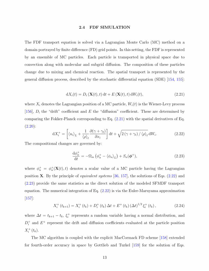
general diffusion process, described by the stochastic differential equation (SDE) [154, 155]:

dXi(t) = Di (X(t), t) dt+ E (X(t), t) dWi(t), (2.21)

where Xi denotes the Lagrangian position of a MC particle, Wi(t) is the Wiener-Levy process

[156], Di the “drift” coefficient and E the “diffusion” coefficient. These are determined by

comparing the Fokker-Planck corresponding to Eq. (2.21) with the spatial derivatives of Eq.

(2.20):

dX+i =

[〈ui〉L +

1

〈ρ〉`∂(γ + γt)

∂xi

]dt+

√2 (γ + γt) / 〈ρ〉` dWi. (2.22)

The compositional changes are governed by:

dφ+α

dt= −Ωm

(φ+α − 〈φα〉L

)+ Sα(φ+), (2.23)

where φ+α = φ+

α (X(t), t) denotes a scalar value of a MC particle having the Lagrangian

position X. By the principle of equivalent systems [36, 157], the solutions of Eqs. (2.22) and

(2.23) provide the same statistics as the direct solution of the modeled SFMDF transport

equation. The numerical integration of Eq. (2.22) is via the Euler-Maruyama approximation

[157]:

X+i (tk+1) = X+

i (tk) +D+i (tk) ∆t+ E+ (tk) (∆t)1/2 ξ+

i (tk) , (2.24)

where ∆t = tk+1 − tk, ξ+i represents a random variable having a normal distribution, and

D+i and E+ represent the drift and diffusion coefficients evaluated at the particle position

X+i (tk).

The MC algorithm is coupled with the explicit MacCormack FD scheme [158] extended

for fourth-order accuracy in space by Gottlieb and Turkel [159] for the solution of Eqs.

13

Figure 1: Typical three-dimensional section of the domain in the hybrid simulation. Solid

cubes denote FD points. Spheres denote MC particles. The dashed line represents the

ensemble domain.

14

(2.9–2.12). A typical three-dimensional section of the domain is presented in Fig. 1. The

communication between the two constituents of this hybrid solver is through interpolation

and ensemble averaging. The former is done via simple interpolation of FD values to the

particle positions and the latter is by consideration of an ensemble ofNE particles in a domain

of size ∆3E. This strong coupling of the two solvers makes parallel simulation very challenging.

The number of MC particles required for accurate statistics is usually an order of magnitude

larger than the number of FD points. For each of these particles, the chemical source terms

must be evaluated. In hydrocarbon combustion, this involves a stiff set of coupled nonlinear

ordinary differential equations (ODEs). Even with reduced kinetics models and moderate

Reynolds numbers, serial simulations would require years of computation [13].

2.5 IPLMCFD

In parallel simulations, the domain is typically divided into an ensemble of subdomains, each

assigned to a processor and each containing the same number of FD points and MC particles.

This decomposition is done a priori and usually remains fixed in time (Fig. 2(a)). In addition

to its rather trivial geometrical edge-cut, in such a decomposition, the communications

between the neighboring elements is kept to a minimum. However, it exhibits very poor load

balancing in dealing with chemistry simulations with finite-rate kinetics. As demonstrated

in Fig. 2(b), due to the local nature of chemical reactions, calculations on a few processors

continue while the others remain idle. Regions of high computational cost, as presented in

Fig. 3, correspond to high reaction zones. For compositions in the cold regions, Sα ≈ 0;

so integration of Eq. (2.23) can be performed over a few implicit sub-steps. In the reacting

regions of the flow, this system may be stiff and many implicit sub-steps may be required.

The total walltime each subdomain spends on integration will, therefore, be quite disparate

for uniform decompositions.

A variety of methodologies have been developed to deal with the computationally expen-

sive turbulent combustion simulation. For a flame near equilibrium, the flamelet approxima-

tion has been useful [160]. In this approach, the thermochemical variables are related to the

15

0 20 40 60 80 99

rank

(a)

0 20 40 60 80 1000

5

10

15

20

25

rank

walltime(s)

(b)

Figure 2: (a) Subdomain boundaries and (b) walltime per timestep for each subdomain for

the uniform decomposition.

walltime (ms)

500

600

700

800

900

1000

1100

Figure 3: Instantaneous CPU time in milliseconds spent performing particle integration.

16

mixture fraction, which is a passive scalar variable. This approach reduces the computation

time dramatically. The in situ adaptive tabulation (ISAT) approach [161–166] is another

powerful method which combines table lookup with direct integration to allow treatment of

a broad range of reacting flows. ISAT is based on the concept that many particle composi-

tions of the flow are similar and reappear repeatedly throughout the simulation. Thus direct

integration is conducted once for a given composition and is stored in a table. If a particle’s

composition resides in the table, the lookup combined with interpolation is performed in lieu

of direct integration. This results in a significant reduction of the total computation time

[161]. In theory, the limit of optimal performance would be near that of the flamelet model.

In practice, direct integration for a portion of the particles are required for each iteration,

resulting in a spatial load imbalance.

In the context of parallel simulation, the master-slave strategy is commonly employed to

resolve the spatial load imbalance problem. See, for example, Ref. [167]. In this strategy, one

process (the master) is in charge of assigning and distributing work to the rest (the slaves).

A scalable parallel implementation relies on the ability of the master process to efficiently

manage the distribution. Obviously, this becomes increasingly difficult as the number of

slave processes increases.

The scheme developed here is termed “irregularly portioned Lagrangian Monte Carlo

finite difference” (IPLMCFD). In this scheme, the computational domain is decomposed

into irregularly shaped subdomains. Each subdomain is an entirely self-contained hybrid

Eulerian/Lagrangian flow solver. The communication between the Lagrangian and Eulerian

solvers is purely local, and the shared information among subdomains, typical of FD and MC

methods, is limited to neighbors only. This shared information, corresponding to data that

is calculated on neighboring subdomains but required locally, is stored in extra elements

of each local data array commonly referred to as ghost points [168]. For the FD solver,

these ghost points correspond to the stencils used for differentiation. For the MC solver,

they correspond to the cloud of cells surrounding a given cell, required for interpolation and

ensemble averaging as discussed in §2.4. All communication among subdomains is via the

Message-Passing Interface (MPI) [168]. As outlined in [167], when utilizing more processors

for a fixed problem size, the subdomains become smaller and the ratio of ghost points to

17

local data points increases. At some stage the communication overhead becomes significant

relative to the local computation, and the scalability begins to tail off.

An even distribution of the CPU load is the primary factor in determining the shape of

the subdomains. The CPU time, as depicted in Fig. 3, is fed into a weighted graph parti-

tioning algorithm [169]. This algorithm decomposes the domain such that each subdomain

is responsible for the same amount of work in terms of CPU time. Simultaneously, it aims to

minimize the edge-cuts of each subdomain. A resulting decomposition is presented in Fig.

4(a). The downside to such a decomposition is that the resulting communication among

neighboring subdomains can be quite arbitrary and requires significant bookkeeping. How-

ever, the major advantage is that the computational load is efficiently balanced, as shown

in Fig. 4(b). Further, since each subdomain is a self-contained hybrid solver, it is trivial to

include other cost reducing chemistry solvers, such as ISAT, etc.

The cost of re-balancing the load is characterized by the necessary amount of data mi-

gration between the two decompositions. The spatial distribution of the computational load

depends on the physics of the problem and varies in a transient manner. Ideally, if the

cost of domain decomposition and re-decomposition are zero, each iteration would begin

with a perfectly balanced load. Qualitatively, this temporal deterioration of load balance is

case dependent. An example of the temporal performance of the domain decomposition is

presented in §2.6.1.

2.6 RESULTS

2.6.1 Scalability

The computational efficiency of the IPLMCFD methodology is examined here by its appli-

cation for LES of a premixed Bunsen burner flame [170]. This flame consists of a main jet

(D = 12 mm) having a stoichiometric mixture of methane (CH4) and air. The Reynolds

number of the jet is 22, 400. These simulations are conducted with 2.5× 106 FD points and

2 × 107 MC particles on Kraken, which is a Cray XT5 system with the National Institute

18

0 20 40 60 80 99

rank

(a)

0 20 40 60 80 1000

1

2

3

4

5

6

rank

walltime(s)

(b)

Figure 4: (a) Subdomain boundaries and (b) walltime per timestep for each subdomain for

the IPLMCFD methodology.

19

0 5k 10k0

2k

4k

6k

8k

10k

number of CPU’s, p

t 1/t p

IdealIPLMCFDUnbalanced

(a)

0 5k 10k0

2k

4k

6k

8k

10k

number of CPU’s, p

t 1/t p

Ideal20M30M40M

(b)

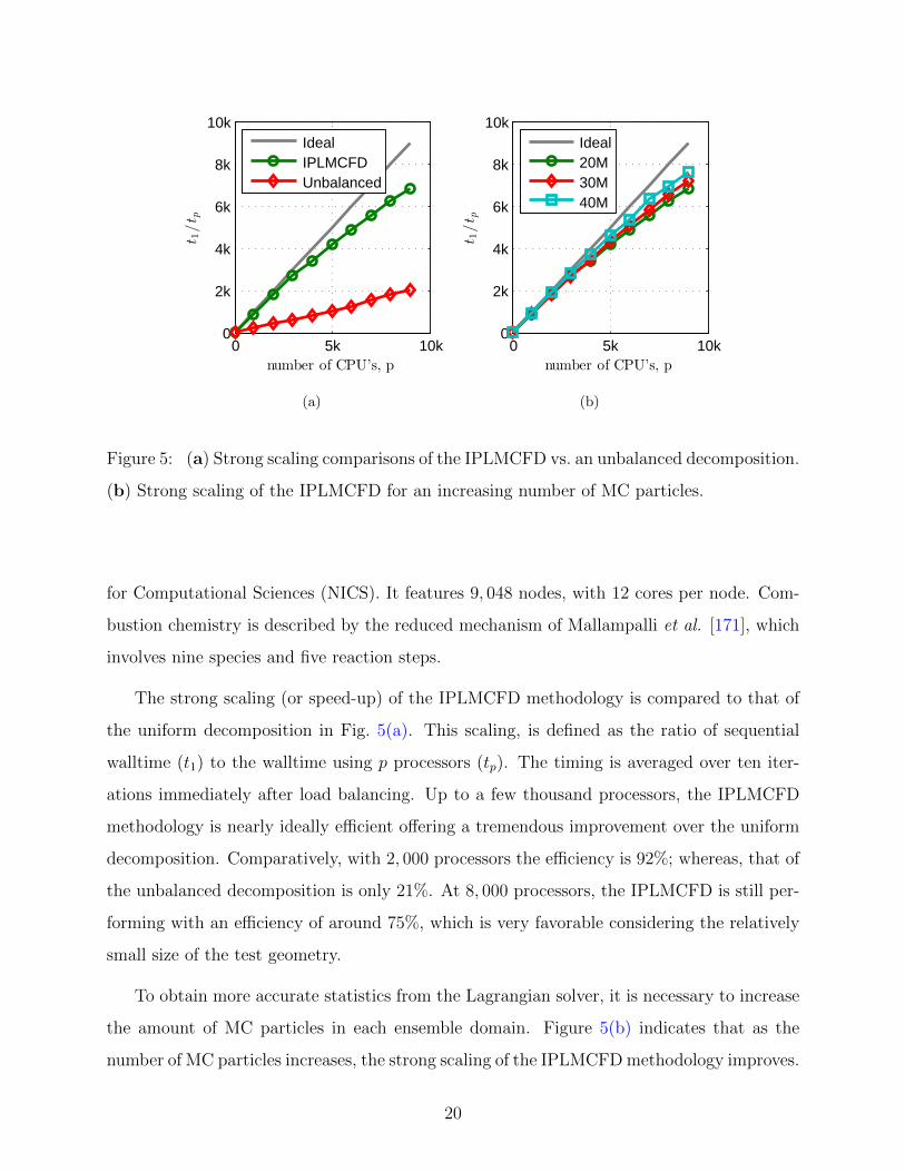
Figure 5: (a) Strong scaling comparisons of the IPLMCFD vs. an unbalanced decomposition.

(b) Strong scaling of the IPLMCFD for an increasing number of MC particles.

for Computational Sciences (NICS). It features 9, 048 nodes, with 12 cores per node. Com-

bustion chemistry is described by the reduced mechanism of Mallampalli et al. [171], which

involves nine species and five reaction steps.

The strong scaling (or speed-up) of the IPLMCFD methodology is compared to that of

the uniform decomposition in Fig. 5(a). This scaling, is defined as the ratio of sequential

walltime (t1) to the walltime using p processors (tp). The timing is averaged over ten iter-

ations immediately after load balancing. Up to a few thousand processors, the IPLMCFD

methodology is nearly ideally efficient offering a tremendous improvement over the uniform

decomposition. Comparatively, with 2, 000 processors the efficiency is 92%; whereas, that of

the unbalanced decomposition is only 21%. At 8, 000 processors, the IPLMCFD is still per-

forming with an efficiency of around 75%, which is very favorable considering the relatively

small size of the test geometry.

To obtain more accurate statistics from the Lagrangian solver, it is necessary to increase

the amount of MC particles in each ensemble domain. Figure 5(b) indicates that as the

number of MC particles increases, the strong scaling of the IPLMCFD methodology improves.

20

0 5k 10k0

0.5

1

1.5

2

2.5

number of CPU’s, p

walltime(s)

UnbalancedIPLMCFD

(a)

0 5k 10k0

0.5

1

1.5

2

2.5

3

number of CPU’s, p

walltime(s)

(b)

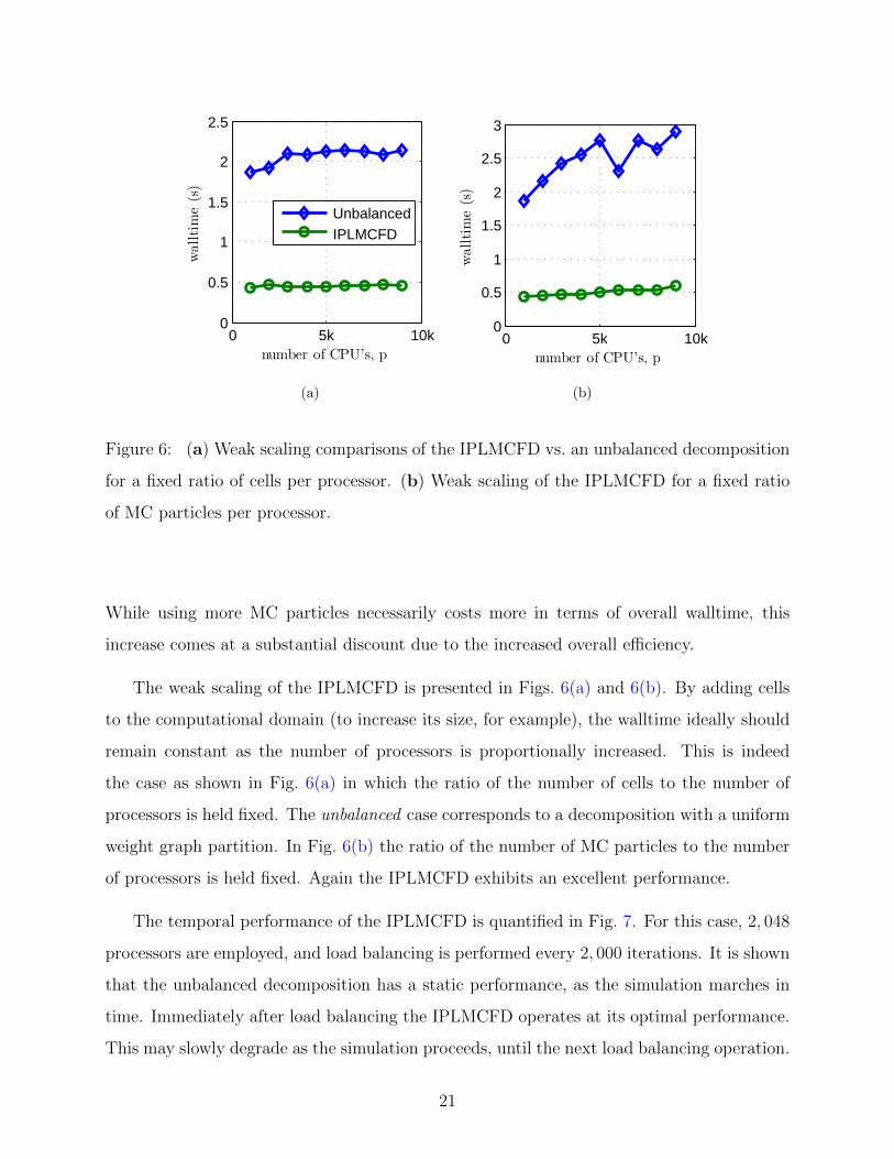
Figure 6: (a) Weak scaling comparisons of the IPLMCFD vs. an unbalanced decomposition

for a fixed ratio of cells per processor. (b) Weak scaling of the IPLMCFD for a fixed ratio

of MC particles per processor.

While using more MC particles necessarily costs more in terms of overall walltime, this

increase comes at a substantial discount due to the increased overall efficiency.

The weak scaling of the IPLMCFD is presented in Figs. 6(a) and 6(b). By adding cells

to the computational domain (to increase its size, for example), the walltime ideally should

remain constant as the number of processors is proportionally increased. This is indeed

the case as shown in Fig. 6(a) in which the ratio of the number of cells to the number of

processors is held fixed. The unbalanced case corresponds to a decomposition with a uniform

weight graph partition. In Fig. 6(b) the ratio of the number of MC particles to the number

of processors is held fixed. Again the IPLMCFD exhibits an excellent performance.

The temporal performance of the IPLMCFD is quantified in Fig. 7. For this case, 2, 048

processors are employed, and load balancing is performed every 2, 000 iterations. It is shown

that the unbalanced decomposition has a static performance, as the simulation marches in

time. Immediately after load balancing the IPLMCFD operates at its optimal performance.

This may slowly degrade as the simulation proceeds, until the next load balancing operation.

21

0 5k 10k 15k 20k1

2

3

4

5

6

7

8

9

iteration

walltime(s)

UnbalancedIPLMCFD

Figure 7: Performance in time of the IPLMCFD vs. an unbalanced decomposition.

The degradation is most pronounced initially, as the solver sweeps the initial condition out

of the domain. The integral of the difference between the unbalanced case and IPLMCFD

over the number of iterations provides the measure of the total walltime savings afforded by

the IPLMCFD (excluding the cost of re-decomposition).

2.6.2 Realizability

The realizability of the IPLMCFD solver is assessed by LES of a turbulent jet flow under

the influence of an exothermic chemical reaction A+ B −→ P + Heat. The rate of reactant

conversion is governed by SA = −ρkAB, where A and B are the mass fractions of species

A and B. The jet has a fuel composition of A∞ = 1 and temperature TA = 300 K. The

coflow has oxidizer composition of B∞ = 1 and temperature TB = 300 K. The heat release,

Q/Cp = 1, 400 K; yielding the adiabatic flame temperature of 1, 000 K. To assess realizability,

the scalar values along with the temperature are presented in the domain of the mixture

fraction. Here the mixture fraction, ξ, is defined such that ξ = 1 in the fuel stream, ξ = 0 in

the oxidizer stream and ξ = 0.5 on the flame surface.

22

0 0.5 10

0.2

0.4

0.6

0.8

1

〈ξ〉L

〈A〉 L

0 0.5 10

0.2

0.4

0.6

0.8

1

〈ξ〉L

〈B〉 L

Da=102

Da=10−2

0 0.5 10

0.2

0.4

0.6

0.8

1

〈ξ〉L

〈P〉 L

0 0.5 1200

400

600

800

1000

〈ξ〉L

〈T〉 L

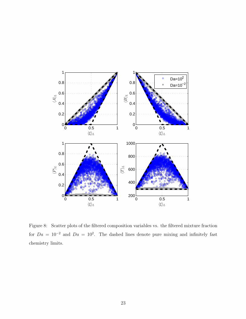
Figure 8: Scatter plots of the filtered composition variables vs. the filtered mixture fraction

for Da = 10−2 and Da = 102. The dashed lines denote pure mixing and infinitely fast

chemistry limits.

23

0 0.2 0.4 0.6 0.8 10

0.2

0.4

0.6

0.8

1

〈ξ〉L

〈Z3〉 L

Figure 9: Scatter plot comparing Z3 vs. the mixture fraction for Da = 102.

The reaction rate (k) is parameterized in terms of the Damkohler number, Da = ρ0L0ku0

,

where ρ0, L0 and u0 represent a reference density, length and velocity respectively. As shown

in Fig. 8, two cases are considered: a (relatively) slow reaction rate (Da = 10−2) and a

fast rate (Da = 102). For the former, the composition is close to that of pure mixing. For

the latter, the composition is close to that of infinitely fast reaction. For other finite values

of Da, the realizable region include the states between the pure mixing and infinitely fast

chemistry limits [44].

Transport of three Shvab-Zeldovich conserved scalars are also considered [43, 44]:

Z1 =A + P

r+1

A∞, Z2 =

B + rPr+1− B∞

−B∞, Z3 =

Cp

Q(T − TB) + A

Cp

Q(TA − TB) + A∞

(2.25)

The consistency of a conserved scalar with the mixture fraction is shown to be nearly perfectly

correlated in Fig. 9 for the case when Da = 102. The results for the case of Da = 10−2 and

the other conserved scalars are similar; thus are not presented.

24

2.6.3 Consistency and Reliability

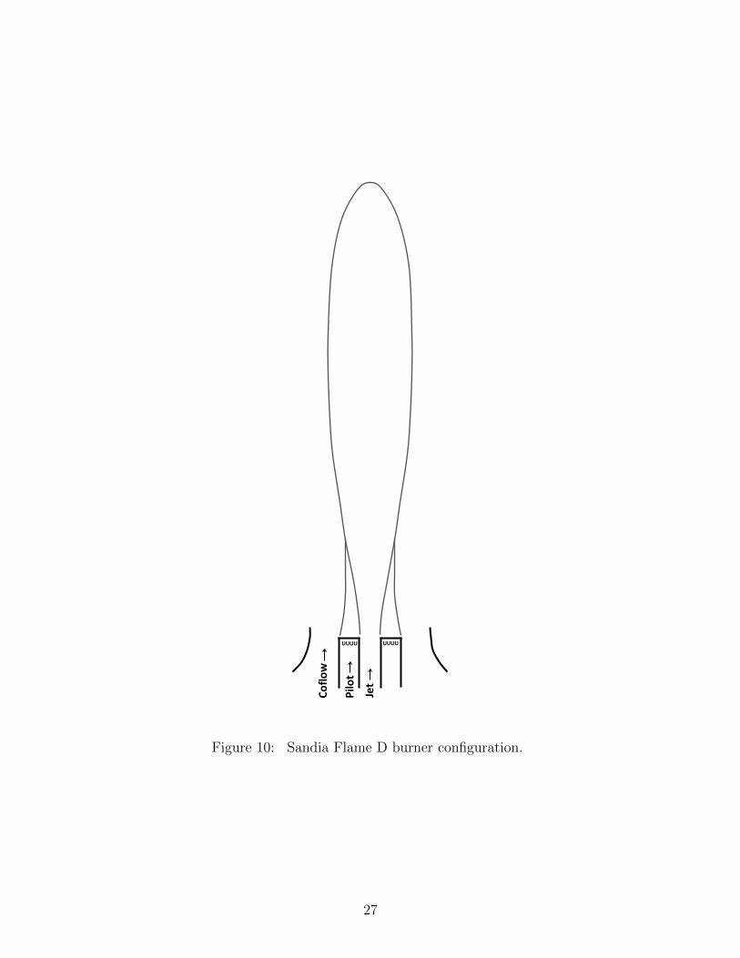
To demonstrate the predictive capability of the IPLMCFD methodology, sample results are

presented for the simulation of a turbulent nonpremixed piloted flame. Sandia Flame D

[172–174] is considered for this purpose. This flame consists of a main fuel jet (D = 7.2 mm)

composed of a mixture of 25% methane (CH4) and 75% air by volume at a temperature of

294 K. The jet has a bulk velocity of 49.6 m/s and a Reynolds number of 22, 400. The fuel

jet is surrounded by a lean pilot mixture of C2H2, H2, air, CO2 and N2 at 1, 880 K. The

measured axial velocity of the pilot gases at the burner exit is 11.4 m/s. The jet and pilot

are surrounded by a coflow of air at 291 K with an axial velocity of 0.9 m/s. A schematic of

the burner is presented in Fig. 10.

The simulation was conducted on a uniformly spaced, three-dimensional Cartesian mesh.

The number of grid points in each coordinate direction is 101 × 101 × 101, mapping to a

physical space of size 20D×10D×10D. An odd number of grid points is used to ensure that

a point lies along the centerline of jet. The filter size is set as ∆G = 2 (∆x∆y∆z)1/3, where

∆x, ∆y and ∆z are the grid spacing in each coordinate direction. The model parameters

used are given in Table 1.

To describe the chemistry, finite-rate kinetics are employed via the augmented reduced

mechanism of Sung et al. [175]. This mechanism was developed for methane oxidation from

GRI-Mech 1.2 [176, 177]. It features 16 species and 12 lumped reaction steps which are

presented in Table 2. The inlet boundary conditions corresponding to the thermochemistry

are adapted from Xu and Pope [178] and are presented in Table 3.

Due to the hybrid nature of the IPLMCFD methodology, some of the thermochemi-

cal transport variables are available from both the Eulerian and Lagrangian solvers. This

redundancy is very useful to examine the solvers’ consistency. Figure 11(a) shows the in-

stantaneous contour plots of the filtered mixture fraction as obtained by both solvers. As

shown in Fig. 11(b), the consistency is convincing.

For the purpose of flow visualization, Fig. 12 presents isosurfaces of the mixture fraction,

temperature and mass fraction of carbon dioxide. Highlighted in this figure are coherent

structures, and the relationship among some of the thermochemical variables of interest.

25

In Figs. 13 - 16 flow statistics are compared with experimental data. These statistics

are generated by long-time averaging the instantaneous values of various thermochemical

flow variables. The initial condition is allowed to sweep through the computational domain

before statistics are collected. In this way, approximately 45, 000 samples were collected. In

the referenced figures 〈Q〉L denotes the time averaged mean of the Favre filtered variable

Q. In general, the agreement with experimental data is excellent. In Fig. 16 there is a

modest over-prediction of the temperature as compared to the experiment. This correlates

with the profiles of methane and oxygen (Fig. 15) which are under-predicted at the same

location. Thus, the simulation is predicting more complete combustion at this location.

This observation agrees with the profile of carbon monoxide, a product gas of hydrocarbon

combustion, which is shown to be over-predicted at the same location.

26

Pilo

t

Coflo

w

Jet

UUUU UUUU

Figure 10: Sandia Flame D burner configuration.

27

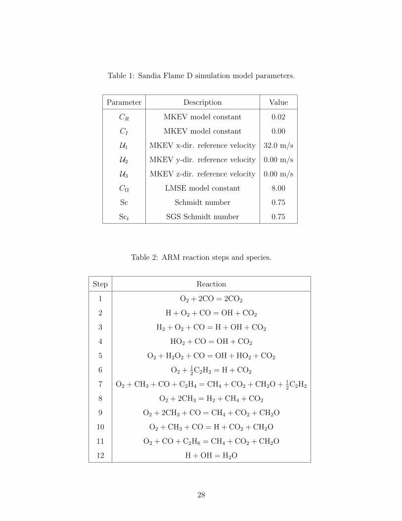
Table 1: Sandia Flame D simulation model parameters.

Parameter Description Value

CR MKEV model constant 0.02

CI MKEV model constant 0.00

U1 MKEV x-dir. reference velocity 32.0 m/s

U2 MKEV y-dir. reference velocity 0.00 m/s

U3 MKEV z-dir. reference velocity 0.00 m/s

CΩ LMSE model constant 8.00

Sc Schmidt number 0.75

Sct SGS Schmidt number 0.75

Table 2: ARM reaction steps and species.

Step Reaction

1 O2 + 2CO = 2CO2

2 H + O2 + CO = OH + CO2

3 H2 + O2 + CO = H + OH + CO2

4 HO2 + CO = OH + CO2

5 O2 + H2O2 + CO = OH + HO2 + CO2

6 O2 + 12C2H2 = H + CO2

7 O2 + CH3 + CO + C2H4 = CH4 + CO2 + CH2O + 12C2H2

8 O2 + 2CH3 = H2 + CH4 + CO2

9 O2 + 2CH3 + CO = CH4 + CO2 + CH2O

10 O2 + CH3 + CO = H + CO2 + CH2O

11 O2 + CO + C2H6 = CH4 + CO2 + CH2O

12 H + OH = H2O

28

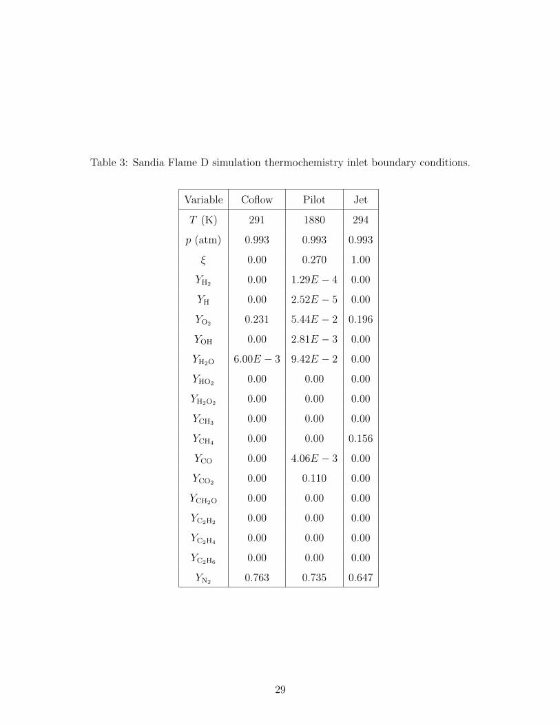
Table 3: Sandia Flame D simulation thermochemistry inlet boundary conditions.

Variable Coflow Pilot Jet

T (K) 291 1880 294

p (atm) 0.993 0.993 0.993

ξ 0.00 0.270 1.00

YH2 0.00 1.29E − 4 0.00

YH 0.00 2.52E − 5 0.00

YO2 0.231 5.44E − 2 0.196

YOH 0.00 2.81E − 3 0.00

YH2O 6.00E − 3 9.42E − 2 0.00

YHO2 0.00 0.00 0.00

YH2O2 0.00 0.00 0.00

YCH3 0.00 0.00 0.00

YCH4 0.00 0.00 0.156

YCO 0.00 4.06E − 3 0.00

YCO2 0.00 0.110 0.00

YCH2O 0.00 0.00 0.00

YC2H2 0.00 0.00 0.00

YC2H4 0.00 0.00 0.00

YC2H6 0.00 0.00 0.00

YN2 0.763 0.735 0.647

29

〈ξFD〉L

0

0.2

0.4

0.6

0.8

1

〈ξMC〉L

(a)

0 0.2 0.4 0.6 0.8 10

0.2

0.4

0.6

0.8

1

〈ξFD〉L

〈ξM

C〉 L

(b)

Figure 11: Comparison of the mixture fraction as calculated by the FD solver and the MC

solver. (a) Visual comparison of a slice of the domain. (b) Scatter plot comparing the entire

domain.

30

Figure 12: Isosurfaces of the mixture fraction, temperature and mass fraction of CO2.

31

0

0.25

0.50

0.75

1.00

x/D = 3

〈ξ〉 L

0

0.06

0.12

0.18

0.24

〈YO

2〉 L

0

0.03

0.06

0.09

0.12

〈YCO

2〉 L

0 0.5 1 1.5 2 2.5

0

0.025

0.050

0.075

0.100

r/D

〈YH

2O〉 L

Figure 13: Radial profiles of the mean mixture fraction and the mean O2, CO2 and H2O

mass fractions at x/D = 3. —IPLMCFD, • Experiment.

32

300

800

1300

1800

2300x/D = 3

〈T〉 L

0

0.040

0.080

0.120

0.160

〈YCH

4〉 L

0

0.015

0.030

0.045

0.060

〈YCO〉 L

0 0.5 1 1.5 2 2.5

0.640

0.670

0.700

0.730

0.760

r/D

〈YN

2〉 L

Figure 14: Radial profiles of the mean temperature and the mean CH4, CO and N2 mass

fractions at x/D = 3. —IPLMCFD, • Experiment.

33

0

0.25

0.50

0.75

1.00

x/D = 7.5

〈ξ〉 L

0

0.06

0.12

0.18

0.24

〈YO

2〉 L

0

0.03

0.06

0.09

0.12

〈YCO

2〉 L

0 0.5 1 1.5 2 2.5

0

0.025

0.050

0.075

0.100

r/D

〈YH

2O〉 L

Figure 15: Radial profiles of the mean mixture fraction and the mean O2, CO2 and H2O

mass fractions at x/D = 7.5. —IPLMCFD, • Experiment.

34

300

800

1300

1800

2300x/D = 7.5

〈T〉 L

0

0.040

0.080

0.120

0.160

〈YCH

4〉 L

0

0.015

0.030

0.045

0.060

〈YCO〉 L

0 0.5 1 1.5 2 2.5

0.640

0.670

0.700

0.730

0.760

r/D

〈YN

2〉 L

Figure 16: Radial profiles of the mean temperature and the mean CH4, CO and N2 mass

fractions at x/D = 7.5. —IPLMCFD, • Experiment.

35

3.0 CONCLUSIONS

The filtered density function (FDF) has proven to be a very powerful and reliable tool for

large eddy simulation (LES) of turbulent reacting flows. One of the major obstacles for a

widespread usage of FDF is its prohibitive computational cost when dealing with complex

chemical kinetics and/or large geometries. In this work, the “irregularly portioned La-

grangian Monte Carlo finite difference” (IPLMCFD) methodology is introduced to mitigate

this cost and to take advantage of modern parallel platforms. This methodology addresses

the load balancing issue by decomposing the computational domain into a series of irregu-

larly shaped and sized subdomains. The resulting algorithm scales to thousands of processors

with an excellent efficiency. The realizability, consistency and the predictive capability of

the FDF are assessed by LES of several turbulent reacting flow configurations.

Future work on the IPLMCFD methodology is recommended to be focused on the fol-

lowing areas:

1. Applications to more complex test cases.

2. Incorporation of more advanced FDF models.

3. Development of an efficient load re-balancing procedure.

4. Improvement in scalability through hybrid parallelism.

3.1 FURTHER APPLICATIONS

The IPLMCFD is recommended to be applied for LES of more complex reacting flows.

Two particular cases are recommended for immediate applications. The first is a turbulent

36

lifted hydrogen jet flame in a heated coflow. This case has been the subject of recent direct

numerical simulation (DNS) [179]. The flame is auto-ignited and is lifted, thus it provides a

good example of partially premixed combustion. The second case is based on the transverse

hydrogen jet issuing perpendicularly into a cross-flow of heated air as considered by DNS

[180]. The cross-flow is over a wall boundary which will present a challenge for LES. Both

cases involve hydrogen fuel, which offers a departure from the hydrocarbon combustion as

considered here. Eventually, the methodology can be applied for LES of practical problems

[145].

3.2 OTHER FDF CLOSURES

The scalar filtered mass density function (SFMDF), is applicable to low-speed reacting flows.

The IPLMCFD can be extended to offer a scalable algorithm for treatment of high-speed

flows including hypersonics. This involves establishing a general framework for the inclusion

of additional FDF models into IPLMCFD. In doing so, the energy-pressure-velocity-scalar

filtered mass density function (EPVS-FMDF) [11, 12] will allow the treatment of high-speed

reacting flows. Also, more precise FDF models for low-speed reacting flows, such as the

velocity-scalar (VSFMDF) [9] and the frequency-velocity-scalar (FVS-FMDF) [10] can be

included as well.

3.3 DYNAMIC PARTITIONING

At present, the partitioning and re-partitioning of the domain into load balanced, irregularly

shaped subdomains is performed at user-defined intervals. This is not a highly efficient

process as it involves saving the current state of the simulation and restarting with the

new decomposition. It is recommended to develop an efficient dynamic load re-balancing

procedure which aims to minimize the data migration between the existing decomposition

and a new decomposition, and to do so without halting the simulation. This can be achieved

through the utilization of existing data management and re-partitioning tools [181, 182].

37

0 1k 2k 3k 4k 5k0

1k

2k

3k

4k

5k

number of CPU’s, p

t 1/t p

IdealIPLMCFD

Figure 17: Strong scaling of the IPLMCFD with only one core per a node utilized.

3.4 HYBRID PARALLELISM

A relatively longer term goal is to exploit the multi-core hybrid architecture of the modern

supercomputers through hybrid parallelism. In this case, distributed parallelism will be

utilized among the nodes via MPI as in the current implementation. While shared parallelism

will be utilized among the cores residing on a node via OpenMP [183]. In an effort to assess

how the IPLMCFD scales on a purely node based level, the strong scaling analysis of §2.6.1

was repeated utilizing only one core per a node. The results are presented in Fig. 17, and

indicate that excellent strong scaling is achieved for distributed parallelism utilizing 5, 000

nodes. These results are from simulations on Kraken, which is a Cray XT5 system with the

National Institute for Computational Sciences (NICS) featuring 9, 048 nodes, with 12 cores

per node. Thus if all cores per a node can be efficiently utilized via shared parallelism, Fig.

17 indicates that IPLMCFD will scale to 60, 000 cores.

38

BIBLIOGRAPHY

[1] Givi, P., Filtered Density Function for Subgrid Scale Modeling of Turbulent Combus-tion, AIAA J., 44(1):16–23 (2006).

[2] Givi, P., Model-Free Simulations of Turbulent Reactive Flows, Prog. Energ. Combust.,15(1):1–107 (1989).

[3] Pope, S. B., Computations of Turbulent Combustion: Progress and Challenges, Proc.Combust. Inst., 23(1):591–612 (1990).

[4] Ansari, N., Jaberi, F. A., Sheikhi, M. R. H., and Givi, P., Filtered Density Functionas a Modern CFD Tool, in Maher, A. R. S., editor, Engineering Applications ofComputational Fluid Dynamics: Volume 1, Chapter 1, pp. 1–22, International Energyand Environment Foundation, 2011.

[5] Colucci, P. J., Jaberi, F. A., Givi, P., and Pope, S. B., Filtered Density Functionfor Large Eddy Simulation of Turbulent Reacting Flows, Phys. Fluids, 10(2):499–515(1998).

[6] Jaberi, F. A., Colucci, P. J., James, S., Givi, P., and Pope, S. B., Filtered MassDensity Function for Large-Eddy Simulation of Turbulent Reacting Flows, J. FluidMech., 401:85–121 (1999).

[7] Gicquel, L. Y. M., Givi, P., Jaberi, F. A., and Pope, S. B., Velocity Filtered DensityFunction for Large Eddy Simulation of Turbulent Flows, Phys. Fluids, 14(3):1196–1213 (2002).

[8] Sheikhi, M. R. H., Drozda, T. G., Givi, P., and Pope, S. B., Velocity-Scalar Fil-tered Density Function for Large Eddy Simulation of Turbulent Flows, Phys. Fluids,15(8):2321–2337 (2003).

[9] Sheikhi, M. R. H., Givi, P., and Pope, S. B., Velocity-Scalar Filtered Mass Den-sity Function for Large Eddy Simulation of Turbulent Reacting Flows, Phys. Fluids,19(9):095106 (2007).

39

[10] Sheikhi, M. R. H., Givi, P., and Pope, S. B., Frequency-Velocity-Scalar FilteredMass Density Function for Large Eddy Simulation of Turbulent Flows, Phys. Fluids,21(7):075102 (2009).

[11] Nik, M. B., Givi, P., Madnia, C. K., and Pope, S. B., EPVS-FMDF for LES ofHigh-Speed Turbulent Flows, in 50th AIAA Aerospace Sciences Meeting including theNew Horizons Forum and Aerospace Exposition, pp. 1–12, Nashville, TN, 2012, AIAA,AIAA-2012-117.

[12] Nik, M. B., VS-FMDF and EPVS-FMDF for Large Eddy Simulation of TurbulentFlows, Ph.D. Thesis, Department of Mechanical Engineering and Materials Science,University of Pittsburgh, Pittsburgh, PA, 2012.

[13] Yilmaz, S. L., Nik, M. B., Sheikhi, M. R. H., Strakey, P. A., and Givi, P., An IrregularlyPortioned Lagrangian Monte Carlo Method for Turbulent Flow Simulation, J. Sci.Comput., 47(1):109–125 (2011).

[14] Pope, S. B., Turbulent Flows, Cambridge University Press, Cambridge, U.K., 2000.

[15] Menon, S., Subgrid Combustion Modelling for Large-Eddy Simulations, Int. J. EngineRes., 1(2):209–227 (2000).

[16] Bilger, R. W., Future Progress in Turbulent Combustion Research, Prog. Energ.Combust., 26(4–6):367–380 (2000).

[17] Veynante, D. and Vervisch, L., Turbulent Combustion Modeling, Prog. Energ. Com-bust., 28(3):193–266 (2002).

[18] Bilger, R. W., Pope, S. B., Bray, K. N. C., and Driscoll, J. F., Paradigms in TurbulentCombustion Research, Proc. Combust. Inst., 30(1):21–42 (2005).

[19] Pitsch, H., Large-Eddy Simulation of Turbulent Combustion, Annu. Rev. Fluid Mech.,38:453–482 (2006).

[20] Echekki, T. and Mastorakos, E., editors, Turbulent Combustion Modeling: Advances,New Trends and Perspectives, Fluid Mechanics and Its Applications, Vol. 95, SpringerNetherlands, 2011.

[21] Williams, F. A., Turbulent Combustion, in Buckmaster, J. D., editor, The Mathematicsof Combustion, Frontiers in Applied Mathematics, SIAM, Philadelphia, PA, 1985.

[22] Peters, N. and Williams, F. A., Liftoff Characteristics of Turbulent Jet DiffusionFlames, AIAA J., 21(3):423–429 (1983).

[23] Schumann, U., Large Eddy Simulation of Turbulent Diffusion with Chemical Reactionsin the Convective Boundary Layer, Atmos. Environ., 23(8):1713–1726 (1989).

40

[24] Libby, P. A. and Williams, F. A., editors, Turbulent Reacting Flows, Topics in AppliedPhysics, Vol. 44, Springer-Verlag, Heidelberg, 1980.

[25] Brodkey, R. S., editor, Turbulence in Mixing Operations: Theory and Application toMixing and Reaction, Academic Press, New York, NY, 1975.

[26] Hill, J. C., Homogeneous Turbulent Mixing with Chemical Reaction, Annu. Rev. FluidMech., 8:135–161 (1976).

[27] Frankel, S. H., Adumitroaie, V., Madnia, C. K., and Givi, P., Large Eddy Simulationsof Turbulent Reacting Flows by Assumed PDF Methods, in Ragab, S. A. and Piomelli,U., editors, Engineering Applications of Large Eddy Simulations, pp. 81–101, ASME,FED-Vol. 162, New York, NY, 1993.

[28] Meeder, J. P. and Nieuwstadt, F. T. M., Subgrid-Scale Segregation of ChemicallyReactive Species in a Neutral Boundary Layer, in Chollet, J.-P., Voke, P. R., andKleiser, L., editors, Direct and Large-Eddy Simulation II, ERCOFTAC Series, Vol. 5,pp. 301–310, Springer Netherlands, 1997.

[29] Tennekes, H. and Lumley, J. L., A First Course in Turbulence, MIT Press, Cambridge,MA, 1972.

[30] Hinze, J. O., Turbulence, McGraw Hill Book Company, New York, NY, 1975.

[31] Wilcox, D. C., Turbulence Modeling for CFD, DCW Industries, Inc., La Canada, CA,third edition, 2006.

[32] Toor, H. L., Mass Transfer in Dilute Turbulent and Non-Turbulent Systems withRapid Irreversible Reactions and Equal Diffusivities, AIChE J., 8(1):70–78 (1962).

[33] Dopazo, C., Non-Isothermal Turbulent Reactive Flows: Stochastic Approaches, Ph.D.Thesis, Department of Mechanical Engineering, State University of New York at StonyBrook, Buffalo, NY, 1973.

[34] Pope, S. B., The Statistical Theory of Turbulent Flames, Phil. Trans. R. Soc. Lond.A, 291(1384):529–568 (1979).

[35] O’Brien, E. E., The Probability Density Function (PDF) Approach to Reacting Turbu-lent Flows, in Libby, P. and Williams, F., editors, Turbulent Reacting Flows, Topics inApplied Physics, Vol. 44, Chapter 5, pp. 185–218, Springer Berlin / Heidelberg, 1980.

[36] Pope, S. B., PDF Methods for Turbulent Reactive Flows, Prog. Energ. Combust.,11(2):119–192 (1985).

[37] Kollmann, W., The PDF Approach to Turbulent Flow, Theor. Comp. Fluid Dyn.,1(5):249–285 (1990).

41

[38] Lundgren, T. S., Distribution Functions in the Statistical Theory of Turbulence, Phys.Fluids, 10(5):969–975 (1967).

[39] Lundgren, T. S., Model Equation for Nonhomogeneous Turbulence, Phys. Fluids,12(3):485–497 (1969).

[40] Madnia, C. K. and Givi, P., Direct Numerical Simulation and Large Eddy Simulationof Reacting Homogeneous Turbulence, in Galperin, B. and Orszag, S. A., editors,Large Eddy Simulation of Complex Engineering and Geophysical Flows, Chapter 15,pp. 315–346, Cambridge University Press, Cambridge, England, 1993.

[41] Burke, S. P. and Schumann, T. E. W., Diffusion Flames, Ind. Eng. Chem., 20(10):998–1004 (1928).

[42] Williams, F. A., Structure of Flamelets in Turbulent Reacting Flows and Influencesof Combustion on Turbulence Fields, in Borghi, R. and Murthy, S. N. B., editors,Turbulent Reactive Flows, Lecture Notes in Engineering, Vol. 40, pp. 195–212, SpringerUS, 1989.

[43] Bilger, R. W., Turbulent Flows with Nonpremixed Reactants, in Libby, P. andWilliams, F., editors, Turbulent Reacting Flows, Topics in Applied Physics, Vol. 44,Chapter 3, pp. 65–113, Springer Berlin / Heidelberg, 1980.

[44] Poinsot, T. and Veynante, D., Theoretical and Numerical Combustion, R. T. Edwards,Inc., Philadelphia, PA, third edition, 2011.

[45] Peters, N., Laminar Diffusion Flamelet Models in Non-Premixed Turbulent Combus-tion, Prog. Energ. Combust., 10(3):319–339 (1984).

[46] Cook, A. W., Riley, J. J., and Kosaly, G., A Laminar Flamelet Approach to Subgrid-Scale Chemistry in Turbulent Flows, Combust. Flame, 109(3):332–341 (1997).

[47] DesJardin, P. E. and Frankel, S. H., Large Eddy Simulation of a Nonpremixed ReactingJet: Application and Assessment of Subgrid-Scale Combustion Models, Phys. Fluids,10(9):2298–2314 (1998).

[48] de Bruyn Kops, S. M., Riley, J. J., Kosaly, G., and Cook, A. W., Investigation of Mod-eling for Non-Premixed Turbulent Combustion, Flow Turbul. Combust., 60(1):105–122(1998).

[49] Cook, A. W. and Riley, J. J., Subgrid-Scale Modeling for Turbulent Reacting Flows,Combust. Flame, 112(4):593–606 (1998).

[50] Pitsch, H. and Steiner, H., Large-Eddy Simulation of a Turbulent Piloted Methane/AirDiffusion Flame (Sandia Flame D), Phys. Fluids, 12(10):2541–2554 (2000).

[51] Muradoglu, M., Liu, K., and Pope, S. B., PDF Modeling of a Bluff-Body StabilizedTurbulent Flame, Combust. Flame, 132(1–2):115–137 (2003).

42

[52] Sheikhi, M. R. H., Drozda, T. G., Givi, P., Jaberi, F. A., and Pope, S. B., Large EddySimulation of a Turbulent Nonpremixed Piloted Methane Jet Flame (Sandia FlameD), Proc. Combust. Inst., 30(1):549–556 (2005).

[53] Drozda, T. G., Sheikhi, M. R. H., Madnia, C. K., and Givi, P., Developments inFormulation and Application of the Filtered Density Function, Flow Turbul. Combust.,78(1):35–67 (2007).

[54] Nik, M. B., Yilmaz, S. L., Givi, P., Sheikhi, M. R. H., and Pope, S. B., Simula-tion of Sandia Flame D Using Velocity-Scalar Filtered Density Function, AIAA J.,48(7):1513–1522 (2010).

[55] Klimenko, A. Y., Multicomponent Diffusion of Various Admixtures in Turbulent Flow,Fluid Dyn., 25(3):327–334 (1990).

[56] Bilger, R. W., Conditional Moment Closure for Turbulent Reacting Flow, Phys. Fluids,5(2):436–444 (1993).

[57] Bushe, W. K. and Steiner, H., Conditional Moment Closure for Large Eddy Simulationof Nonpremixed Turbulent Reacting Flows, Phys. Fluids, 11(7):1896–1906 (1999).

[58] Steiner, H. and Bushe, W. K., Large Eddy Simulation of a Turbulent Reacting Jetwith Conditional Source-Term Estimation, Phys. Fluids, 13(3):754–759 (2001).

[59] Navarro-Martinez, S., Kronenburg, A., and Di Mare, F., Conditional Moment Closurefor Large Eddy Simulations, Flow Turbul. Combust., 75(1–4):245–274 (2005).

[60] Navarro-Martinez, S. and Kronenburg, A., LES-CMC Simulations of a TurbulentBluff-Body Flame, Proc. Combust. Inst., 31(2):1721–1728 (2007).

[61] Navarro-Martinez, S. and Kronenburg, A., LES-CMC Simulations of a Lifted MethaneFlame, Proc. Combust. Inst., 32(1):1509–1516 (2009).

[62] Garmory, A. and Mastorakos, E., Capturing Localised Extinction in Sandia Flame Fwith LES-CMC, Proc. Combust. Inst., 33(1):1673–1680 (2011).

[63] Stankovic, I., Triantafyllidis, A., Mastorakos, E., Lacor, C., and B.Merci, Simulationof Hydrogen Auto-Ignition in a Turbulent Co-flow of Heated Air with LES and CMCApproach, Flow Turbul. Combust., 86(3–4):689–710 (2011).

[64] Stankovic, I., Mastorakos, E., and Merci, B., LES-CMC Simulations of Different Auto-Ignition Regimes of Hydrogen in a Hot Turbulent Air Co-flow, Flow Turbul. Combust.,90(3):583–604 (2013).

[65] Siwaborworn, P. and Kronenburg, A., Conservative Implementation of LES-CMC forTurbulent Jet Flames, in Nagel, W. E., Kroner, D. H., and Resch, M. M., editors,High Performance Computing in Science and Engineering ’12, pp. 159–173, SpringerBerlin Heidelberg, 2013.

43

[66] Klimenko, A. Y. and Pope, S. B., The Modeling of Turbulent Reactive Flows Basedon Multiple Mapping Conditioning, Phys. Fluids, 15(7):1907–1925 (2003).

[67] Cook, A. W. and Riley, J. J., A Subgrid Model for Equilibrium Chemistry in TurbulentFlows, Phys. Fluids, 6(8):2868–2870 (1994).

[68] Jimenez, J., Linan, A., Rogers, M. M., and Higuera, F. J., A priori Testing of SubgridModels for Chemically Reacting Non-Premixed Turbulent Shear Flows, J. Fluid Mech.,349:149–171 (1997).

[69] Wall, C., Boersma, B. J., and Moin, P., An Evaluation of the Assumed Beta ProbabilityDensity Function Subgrid-Scale Model for Large Eddy Simulation of Nonpremixed,Turbulent Combustion with Heat Release, Phys. Fluids, 12(10):2522–2529 (2000).

[70] Johnson, N. L., Systems of Frequency Curves Generated by Methods of Translation,Biometrika, 36:149–176 (1949).

[71] Pierce, C. D. and Moin, P., Progress-Variable Approach for Large-Eddy Simulation ofNon-Premixed Turbulent Combustion, J. Fluid Mech., 504:73–97 (2004).

[72] Mahesh, K., Constantinescu, G., Apte, S., Iaccarino, G., Ham, F., and Moin, P., Large-Eddy Simulation of Reacting Turbulent Flows in Complex Geometries, J. Appl. Mech.,73(3):374–381 (2005).

[73] You, D., Ham, F., and Moin, P., Large-Eddy Simulation Analysis of Turbulent Com-bustion in a Gas Turbine Engine Combustor, in Annual Research Briefs – 2008, pp.219–230, Center for Turbulence Research, Stanford, CA, 2008.

[74] Kerstein, A. R., A Linear-Eddy Model of Turbulent Scalar Transport and Mixing,Combust. Sci. Technol., 60(4–6):391–421 (1988).

[75] Kerstein, A. R., Linear-Eddy Modeling of Turbulent Transport. II: Application toShear Layer Mixing, Combust. Flame, 75(3–4):397–413 (1989).

[76] Kerstein, A. R., Linear-Eddy Modelling of Turbulent Transport. Part 3. Mixing andDifferential Molecular Diffusion in Round Jets, J. Fluid Mech., 216:411–435 (1990).

[77] Kerstein, A. R., Linear-Eddy Modelling of Turbulent Transport. Part 6. Microstructureof Diffusive Scalar Mixing Fields, J. Fluid Mech., 231:361–394 (1991).

[78] Kerstein, A. R., Linear-Eddy Modeling of Turbulent Transport. Part 4. Structure ofDiffusion Flames, Combust. Sci. Technol., 81(1–3):75–96 (1992).

[79] McMurtry, P. A., Menon, S., and Kerstein, A. R., A Linear Eddy Sub-Grid Model forTurbulent Reacting Flows: Application to Hydrogen-Air Combustion, Proc. Combust.Inst., 24(1):271–278 (1992).

44

[80] Kim, W.-W., Menon, S., and Mongia, H. C., Large-Eddy Simulation of a Gas TurbineCombustor Flow, Combust. Sci. Technol., 143(1–6):25–62 (1999).

[81] Kerstein, A. R., One-Dimensional Turbulence: Model Formulation and Application toHomogeneous Turbulence, Shear Flows, and Buoyant Stratified Flows, J. Fluid Mech.,392:277–334 (1999).

[82] Kerstein, A. R., Ashurst, W. T., Wunsch, S., and Nilsen, V., One-Dimensional Tur-bulence: Vector Formulation and Application to Free Shear Flows, J. Fluid Mech.,447:85–109 (2001).

[83] Kerstein, A. R., One-Dimensional Turbulence: A New Approach to High-FidelitySubgrid Closure of Turbulent Flow Simulations, Comput. Phys. Commun., 148(1):1–16 (2002).

[84] Schmidt, R. C., Kerstein, A. R., Wunsch, S., and Nilsen, V., Near-Wall LES ClosureBased on One-Dimensional Turbulence Modeling, J. Comput. Phys., 186(1):317–355(2003).

[85] McDermott, R. J., Toward One-Dimensional Turbulence Subgrid Closure for Large-Eddy Simulation, Ph.D. Thesis, Department of Chemical Engineering, University ofUtah, Salt Lake City, UT, 2005.

[86] Cao, S. and Echekki, T., A Low-Dimensional Stochastic Closure Model for CombustionLarge-Eddy Simulation, J. Turbul., 9(2):1–35 (2008).

[87] Echekki, T. and Park, J., The LES-ODT Model for Turbulent Premixed Flames,in 48th AIAA Aerospace Sciences Meeting Including the New Horizons Forum andAerospace Exposition, Orlando, FL, 2010, AIAA, AIAA-2010-207.

[88] Schmidt, R., Kerstein, A. R., and McDermott, R., ODTLES: A Multi-scale Modelfor 3D Turbulent Flow Based on One-Dimensional Turbulence Modeling, Comput.Method Appl. M., 199(13–16):865–880 (2010).

[89] Gonzalez-Juez, E. D., Schmidt, R. C., and Kerstein, A. R., ODTLES Simulations ofWall-bounded Flows, Phys. Fluids, 23(12):125102 (2011).

[90] Park, J. and Echekki, T., LES-ODT Study of Turbulent Premixed Interacting Flames,Combust. Flame, 159(2):609–620 (2012).

[91] Mirgolbabaei, H. and Echekki, T., A Novel Principal Component Analysis-based Ac-celeration Scheme for LES-ODT: An a priori Study, Combust. Flame, 160(5):898–908(2013).

[92] Spalding, D. B., Mixing and Chemical Reaction in Steady Confined Turbulent Flames,Proc. Combust. Inst., 13(1):649 – 657 (1971).

45

[93] Spalding, D. B., Development of the Eddy-Break-Up Model of Turbulent Combustion,Proc. Combust. Inst., 16(1):1657–1663 (1977).

[94] Fureby, C. and Lofstrom, C., Large-Eddy Simulations of Bluff Body Stabilized Flames,Proc. Combust. Inst., 25(1):1257–1264 (1994).

[95] Butler, T. D. and O’Rourke, P. J., A Numerical Method for Two Dimensional UnsteadyReacting Flows, Proc. Combust. Inst., 16(1):1503–1515 (1977).

[96] Colin, O., Ducros, F., Veynante, D., and Poinsot, T., A Thickened Flame Model forLarge Eddy Simulation of Turbulent Premixed Combustion, Phys. Fluids, 12(7):1843–1863 (2000).

[97] Charlette, F., Meneveau, C., and Veynante, D., A Power-law Flame Wrinkling Modelfor LES of Premixed Turbulent Combustion Part I: Non-dynamic Formulation andInitial Tests, Combust. Flame, 131(1–2):159–180 (2002).

[98] Charlette, F., Meneveau, C., and Veynante, D., A Power-law Flame Wrinkling Modelfor LES of Premixed Turbulent Combustion Part II: Dynamic Formulation, Combust.Flame, 131(1–2):181–197 (2002).

[99] Boileau, M., Staffelbach, G., Cuenot, B., Poinsot, T., and Berat, C., LES of an IgnitionSequence in a Gas Turbine Engine, Combust. Flame, 154(1–2):2–22 (2008).

[100] Hernandez-Perez, F. E., Yuen, F. T. C., Groth, C. P. T., and Gulder, O. L., LESof a Laboratory-scale Turbulent Premixed Bunsen Flame using FSD, PCM-FPI andThickened Flame Models, Proc. Combust. Inst., 33(1):1365–1371 (2011).

[101] Wang, G., Boileau, M., and Veynante, D., Implementation of a Dynamic ThickenedFlame Model for Large Eddy Simulations of Turbulent Premixed Combustion, Com-bust. Flame, 158(11):2199–2213 (2011).

[102] Kuenne, G., Ketelheun, A., and Janicka, J., LES Modeling of Premixed Combustionusing a Thickened Flame Approach coupled with FGM Tabulated Chemistry, Combust.Flame, 158(9):1750–1767 (2011).

[103] Kerstein, A. R., Ashurst, W. T., and Williams, F. A., Field Equation for InterfacePropagation in an Unsteady Homogeneous Flow Field, Phys. Rev. A, 37(7):2728–2731(1988).

[104] Im, H. G., Lund, T. S., and Ferziger, J. H., Large Eddy Simulation of Turbulent FrontPropagation with Dynamic Subgrid Models, Phys. Fluids, 9(12):3826–3833 (1997).

[105] Pitsch, H. and de Lageneste, L. D., Large-Eddy Simulation of Premixed Turbu-lent Combustion using a Level-Set Approach, Proc. Combust. Inst., 29(2):2001–2008(2002).

46

[106] Pitsch, H., A Consistent Level Set Formulation for Large-Eddy Simulation of PremixedTurbulent Combustion, Combust. Flame, 143(4):587–598 (2005).

[107] Wang, P. and Bai, X., Large Eddy Simulation of Turbulent Premixed Flames usingLevel-Set G-Equation, Proc. Combust. Inst., 30(1):583–591 (2005).

[108] Freitag, M. and Janicka, J., Investigation of a Strongly Swirled Unconfined PremixedFlame using LES, Proc. Combust. Inst., 31(1):1477–1485 (2007).

[109] Moureau, V., Fiorina, B., and Pitsch, H., A Level Set Formulation for PremixedCombustion LES Considering the Turbulent Flame Structure, Combust. Flame,156(4):801–812 (2009).

[110] Zhou, X. Y. and Pereira, J. C. F., Large Eddy Simulation (2D) of a Reacting Plane Mix-ing Layer using Filtered Density Function Closure, Flow Turbul. Combust., 64(4):279–300 (2000).

[111] Heinz, S., On Fokker-Planck Equations for Turbulent Reacting Flows. Part 1. Proba-bility Density Function for Reynolds-Averaged Navier-Stokes Equations, Flow Turbul.Combust., 70(1–4):115–152 (2003).

[112] Raman, V., Pitsch, H., and Fox, R. O., Hybrid Large-Eddy Simulation/LagrangianFiltered-Density-Function Approach for Simulating Turbulent Combustion, Combust.Flame, 143(1–2):56–78 (2005).

[113] Raman, V. and Pitsch, H., Large-Eddy Simulation of a Bluff-Body-Stabilized Non-Premixed Flame using a Recursive Filter-Refinement Procedure, Combust. Flame,142(4):329–347 (2005).

[114] van Vliet, E., Derksen, J. J., and van den Akker, H. E. A., Turbulent Mixing in aTubular Reactor: Assessment of an FDF/LES Approach, AIChE J., 51(3):725–739(2005).

[115] Carrara, M. D. and DesJardin, P. E., A Filtered Mass Density Function Approach forModeling Separated Two-Phase Flows for LES I: Mathematical Formulation, Int. J.Multiphas. Flow, 32(3):365–384 (2006).

[116] Mustata, R., Valio, L., Jimnez, C., Jones, W., and Bondi, S., A Probability DensityFunction Eulerian Monte Carlo Field Method for Large Eddy Simulations: Applicationto a Turbulent Piloted Methane/Air Diffusion Flame (Sandia D), Combust. Flame,145(1–2):88–104 (2006).

[117] Jones, W. P., Navarro-Martinez, S., and Rohl, O., Large Eddy Simulation of HydrogenAuto-Ignition with a Probability Density Function Method, Proc. Combust. Inst.,31(2):1765–1771 (2007).

47

[118] Jones, W. P. and Navarro-Martinez, S., Large Eddy Simulation of Autoignition witha Subgrid Probability Density Function Method, Combust. Flame, 150(3):170–187(2007).

[119] James, S., Zhu, J., and Anand, M. S., Large Eddy Simulation of Turbulent FlamesUsing the Filtered Density Function Model, Proc. Combust. Inst., 31(2):1737–1745(2007).

[120] Chen, J.-Y., A Eulerian PDF Scheme for LES of Nonpremixed Turbulent Combustionwith Second-Order Accurate Mixture Fraction, Combust. Theor. Model., 11(5):675–695 (2007).

[121] McDermott, R. and Pope, S. B., A Particle Formulation for Treating DifferentialDiffusion in Filtered Density Function Methods, J. Comput. Phys., 226(1):947–993(2007).

[122] Raman, V. and Pitsch, H., A Consistent LES/Filtered-Density Function Formulationfor the Simulation of Turbulent Flames with Detailed Chemistry, Proc. Combust. Inst.,31(2):1711–1719 (2007).

[123] Afshari, A., Jaberi, F. A., and Shih, T. I.-P., Large-Eddy Simulations of TurbulentFlows in an Axisymmetric Dump Combustor, AIAA J., 46(7):1576–1592 (2008).

[124] Drozda, T. G., Wang, G., Sankaran, V., Mayo, J. R., Oefelein, J. C., and Barlow,R. S., Scalar Filtered Mass Density Functions in Nonpremixed Turbulent Jet Flames,Combust. Flame, 155(1–2):54–69 (2008).

[125] Reveillon, J. and Vervisch, L., Subgrid-Scale Turbulent Micromixing: Dynamic Ap-proach, AIAA J., 36(3):336–341 (1998).

[126] Cha, C. M. and Trouillet, P., A Subgrid-Scale Mixing Model for Large-Eddy Simula-tion of Turbulent Reacting Flows using the Filtered Density Function, Phys. Fluids,15(6):1496–1504 (2003).

[127] Heinz, S., Unified Turbulence Models for LES and RANS, FDF and PDF Simulations,Theor. Comp. Fluid Dyn., 21(2):99–118 (2007).

[128] Tong, C., Measurements of Conserved Scalar Filtered Density Function in a TurbulentJet, Phys. Fluids, 13(10):2923–2937 (2001).

[129] Wang, D. and Tong, C., Conditionally Filtered Scalar Dissipation, Scalar Diffusion,and Velocity in a Turbulent Jet, Phys. Fluids, 14(7):2170–2185 (2002).

[130] Rajagopalan, A. G. and Tong, C., Experimental Investigation of Scalar-Scalar-Dissipation Filtered Joint Density Function and its Transport Equation, Phys. Fluids,15(1):227–244 (2003).

48

[131] Wang, D., Tong, C., and Pope, S. B., Experimental Study of Velocity Filtered JointDensity Function for Large Eddy Simulation, Phys. Fluids, 16(10):3599–3613 (2004).

[132] Wang, D. and Tong, C., Experimental Study of Velocity-Scalar Filtered Joint DensityFunction for LES of Turbulent Combustion, Proc. Combust. Inst., 30(1):567–574(2005).

[133] Colucci, P. J., Large Eddy Simulation of Turbulent Reactive Flows: Stochastic Rep-resentation of the Subgrid Scale Scalar Fluctutations, Ph.D. Thesis, State Universityof New York at Buffalo, Buffalo, NY, 1998.

[134] Gicquel, L. Y. M., Velocity Filtered Density Function for Large Eddy Simulation ofTurbulent Flows, Ph.D. Thesis, Department of Mechanical Engineering, State Univer-sity of New York at Buffalo, Buffalo, NY, 2001.

[135] Drozda, T. G., Implementation of LES/SFMDF for Prediction of Non-Premixed Tur-bulent Flames, Ph.D. Thesis, Department of Mechanical Engineering, University ofPittsburgh, Pittsburgh, PA, 2005.

[136] Sheikhi, M. R. H., Joint Velocity Scalar Filtered Density Function for Large EddySimulation of Turbulent Reacting Flows, Ph.D. Thesis, Department of MechanicalEngineering, University of Pittsburgh, Pittsburgh, PA, 2005.

[137] Pisciuneri, P. H., Large Eddy Simulation of a Turbulent Nonpremixed Jet Flame Usinga Finite-Rate Chemistry Model, M.S. Thesis, Department of Mechanical Engineeringand Materials Science, University of Pittsburgh, Pittsburgh, PA, 2008.

[138] Yilmaz, S. L., RANS/PDF and LES/FDF for Prediction of Turbulent PremixedFlames, Ph.D. Thesis, Department of Mechanical Engineering and Materials Science,University of Pittsburgh, Pittsburgh, PA, 2008.

[139] Ansari, N., Filtered Density Function for Large Eddy Simulation of Turbulent ReactingFlows on Unstructured Meshes, Ph.D. Thesis, Department of Mechanical Engineeringand Materials Science, University of Pittsburgh, Pittsburgh, PA, 2012.

[140] Otis, C. C., High-Fidelity Simulation of Compressible Flows for Hypersonic PropulsionApplications, Ph.D. Thesis, Department of Mechanical Engineering and MaterialsScience, University of Pittsburgh, Pittsburgh, PA, 2013.

[141] Pisciuneri, P. H., Yilmaz, S. L., Strakey, P. A., and Givi, P., An Irregularly PortionedFDF Simulator, SIAM J. Sci. Comput., (2013), in press.

[142] Pisciuneri, P. H., Yilmaz, S. L., Strakey, P., and Givi, P., An Irregularly PortionedFDF Solver, Bull. Am. Phys. Soc., 56(18):305 (2011).

[143] Pisciuneri, P. H., Yilmaz, S. L., and Givi, P., Petascale FDF Large Eddy Simulationof Reacting Flows, Bull. Am. Phys. Soc., 57(17):123 (2012).

49

[144] Yilmaz, S. L., Ansari, N., Pisciuneri, P. H., Nik, M. B., Otis, C. C., and Givi, P.,Advances in FDF Modeling and Simulation, in 47th AIAA/ASME/SAE/ASEE JointPropulsion Conference & Exhibit, pp. 1–11, San Diego, CA, 2011, AIAA, AIAA-2011-5918.

[145] Yilmaz, S. L., Ansari, N., Pisciuneri, P. H., Nik, M. B., Otis, C. C., and Givi, P.,Applied Filtered Density Function, J. Appl. Fluid Mech., 6(3):311–320 (2013).

[146] Drozda, T. G., Quinlan, J. R., Pisciuneri, P. H., and Yilmaz, S. L., Progress TowardAffordable High Fidelity Combustion Simulations for High-Speed Flows in ComplexGeometries, in 48th AIAA/ASME/SAE/ASEE Joint Propulsion Conference & Exhibit,pp. 1–16, Atlanta, GA, 2012, AIAA, AIAA-2012-4264.

[147] Ansari, N., Pisciuneri, P. H., Strakey, P. A., and Givi, P., Scalar-Filtered Mass-Density-Function Simulation of Swirling Reacting Flows on Unstructured Grids, AIAA J.,50(11):2476–2482 (2012).

[148] Sagaut, P., Large Eddy Simulation for Incompressible Flows, Springer, New York, NY,third edition, 2010.

[149] Vreman, B., Geurts, B., and Kuerten, H., Realizability Conditions for the TurbulentStress Tensor in Large-Eddy Simulation, J. Fluid Mech., 278:351–362 (1994).

[150] Erlebacher, G., Hussaini, M. Y., Speziale, C. G., and Zang, T. A., Toward theLarge-Eddy Simulation of Compressible Turbulent Flows, J. Fluid Mech., 238:155–185(1992).

[151] Bardina, J., Ferziger, J. H., and Reynolds, W. C., Improved Turbulence ModelsBased on Large Eddy Simulation of Homogeneous, Incompressible Turbulent Flows,Department of Mechanical Engineering Report TF-19, Stanford University, Stanford,CA, 1983.

[152] Eidson, T. M., Numerical Simulation of the Turbulent Rayleigh-Benard Problem usingSubgrid Modeling, J. Fluid Mech., 158:245–268 (1985).

[153] Dopazo, C. and O’Brien, E. E., Statistical Treatment of Non-Isothermal ChemicalReactions in Turbulence, Combust. Sci. Technol., 13(1–6):99–122 (1976).

[154] Risken, H., The Fokker-Planck Equation, Methods of Solution and Applications,Springer-Verlag, New York, NY, 1989.

[155] Gardiner, C. W., Handbook of Stochastic Methods for Physics, Chemistry and theNatural Sciences, Springer-Verlag, New York, NY, second edition, 1990.

[156] Karlin, S. and Taylor, H. M., A Second Course in Stochastic Processes, AcademicPress, New York, NY, 1981.

50

[157] Kloeden, P. E. and Platen, E., Numerical Solution of Stochastic Differential Equations,Applications of Mathematics, Vol. 23, Springer, Berlin; New York, third edition, 1999.

[158] MacCormack, R. W., The Effect of Viscosity in Hypervelocity Impact Cratering, J.Spacecraft Rockets, 40(5):757–763 (2003).

[159] Gottlieb, D. and Turkel, E., Dissipative Two-Four Methods for Time-Dependent Prob-lems, Math. Comput., 30(136):703–723 (1976).

[160] Peters, N., Turbulent Combustion, Cambridge University Press, Cambridge, UK, 2000.

[161] Pope, S. B., Computationally Efficient Implementation of Combustion Chemistry usingin situ Adaptive Tabulation, Combust. Theor. Model., 1(1):41–63 (1997).

[162] Singer, M. A. and Pope, S. B., Exploiting ISAT to Solve the Reaction-Diffusion Equa-tion, Combust. Theor. Model., 8(2):361–383 (2004).

[163] Liu, B. J. D. and Pope, S. B., The Performance of in situ Adaptive Tabulation inComputations of Turbulent Flames, Combust. Theor. Model., 9(4):549–568 (2005).

[164] Singer, M. A., Pope, S. B., and Najm, H. N., Modeling Unsteady Reacting Flow withOperator Splitting and ISAT, Combust. Flame, 147(1–2):150–162 (2006).

[165] Singer, M. A., Pope, S. B., and Najm, H. N., Operator-Splitting with ISAT toModel Reacting Flow with Detailed Chemistry, Combust. Theor. Model., 10(2):199–217 (2006).

[166] Hiremath, V., Lantz, S. R., Wang, H., and Pope, S. B., Computationally-Efficient andScalable Parallel Implementation of Chemistry in Simulations of Turbulent Combus-tion, Combust. Flame, 159(10):3096–3109 (2012).

[167] Gourdain, N., Gicquel, L., Montagnac, M., Vermorel, O., Gazaix, M., Staffelbach, G.,Garcia, M., Boussuge, J.-F., and Poinsot, T., High Performance Parallel Computingof Flows in Complex Geometries: I. Methods, Comput. Sci. Disc., 2:015003 (2009).

[168] Gropp, W., Lusk, E., and Skjellum, A., Using MPI: Portable Parallel Programmingwith the Message-Passing Interface, Scientific and Engineering Computation, MITPress, Cambridge, MA, second edition, 1999.

[169] Karypis, G. and Kumar, V., A Fast and High Quality Multilevel Scheme for Parti-tioning Irregular Graphs, SIAM J. Sci. Comput., 20(1):359–392 (1999).

[170] Chen, Y.-C., Peters, N., Schneemann, G. A., Wruck, N., Renz, U., and Mansour, M. S.,The Detailed Flame Structure of Highly Stretched Turbulent Premixed Methane-AirFlames, Combust. Flame, 107(3):223–226 (1996).

51

[171] Mallampalli, H. P., Fletcher, T. H., and Chen, J. Y., Evaluation of CH4/NOx ReducedMechanisms Used for Modeling Lean Premixed Turbulent Combustion of Natural Gas,J. Eng. Gas Turb. Power, 120(4):703–712 (1998).

[172] Sandia National Laboratories, TNF Workshop Website, Piloted Jet Flames, http:

//www.sandia.gov/TNF/pilotedjet.html, 2013.

[173] Barlow, R. S. and Frank, J. H., Effects of Turbulence on Species Mass Fractions inMethane/Air Jet Flames, Proc. Combust. Inst., 27(1):1087–1095 (1998).

[174] Nooren, P. A., Versluis, M., van der Meer, T. H., Barlow, R. S., and Frank, J. H.,Raman-Rayleigh-LIF Measurements of Temperature and Species Concentrations inthe Delft Piloted Turbulent Jet Diffusion Flame, Appl. Phys. B, 71(1):95–111 (2000).

[175] Sung, C. J., Law, C. K., and Chen, J.-Y., An Augmented Reduced Mechanism forMethane Oxidation with Comprehensive Global Parametric Validation, Proc. Com-bust. Inst., 27(1):295–304 (1998).

[176] Frenklach, M., Wang, H., Yu, C.-L., Goldenberg, M., Bowman, C., Hanson, R., David-son, D., Chang, E., Smith, G., Golden, D., Gardiner, W., and Lissianski, V., GRI-Mech1.2, http://diesel.me.berkeley.edu/~gri_mech/new21/version12/text12.html,2013.

[177] Frenklach, M., Wang, H., Goldenberg, M., Smith, G., Golden, D., Bowman, C., Han-son, R., Gardiner, W., and Lissianski, V., GRI-Mech—An Optimized Detailed Chem-ical Reaction Mechanism for Methane Combustion, Technical report, Gas ResearchInstitute, 1995, Report No. GRI-95/0058.

[178] Xu, J. and Pope, S. B., PDF Calculations of Turbulent Nonpremixed Flames withLocal Extinction, Combust. Flame, 123(3):281–307 (2000).

[179] Yoo, C. S., Sankaran, R., and Chen, J. H., Three-Dimensional Direct Numerical Simu-lation of a Turbulent Lifted Hydrogen Jet Flame in Heated Coflow: Flame Stabilizationand Structure, J. Fluid Mech., 640:453–481 (2009).

[180] Grout, R. W., Gruber, A., Yoo, C. S., and Chen, J. H., Direct Numerical Simulationof Flame Stabilization Downstream of a Transverse Fuel Jet in Cross-Flow, Proc.Combust. Inst., 33(1):1629–1637 (2011).

[181] Boman, E., Devine, K., Heaphy, R., Hendrickson, B., Leung, V., Riesen, L. A.,Vaughan, C., Catalyurek, U., Bozdag, D., Mitchell, W., and Teresco, J., Zoltan 3.0:Parallel Partitioning, Load Balancing, and Data-Management Services; User’s Guide,Sandia National Laboratories, Albuquerque, NM, 2007, Tech. Report SAND2007-4748W http://www.cs.sandia.gov/Zoltan/ug_html/ug.html.

52

[182] Karypis, G. and Schloegel, K., ParMETIS: Parallel Graph Partitioning and SparseMatrix Ordering Library, Version 4.0, University of Minnesota, Minneapolis, MN,2013.

[183] OpenMP Architecture Review Board, The OpenMP API Specification for ParallelProgramming, http://openmp.org/wp/, 2013.

53