Embed Size (px)
Citation preview
An Investigation of Wrinkling Behaviour in
Woven Thermoplastic Composite Material
Lu Chen
June 2017
A thesis submitted for the degree of Master of Philosophy
of The Australian National University
© Copyright by Lu Chen 2017
All Rights Reserved

ii

i
Declaration
This thesis is an account of research undertaken between August 2015 and June 2017 at
The Research School of Engineering, College of Engineering and Computer Science,
Australian National University, Canberra, Australia.
Except where acknowledged in the customary manner, the material presented in this
thesis is, to the best of my knowledge, original and has not been submitted in whole or
part for a degree in any university.

ii
iii
Publications
1. L. Chen, S. Kalyanasundaram, "Wrinkling Behavior of a Woven Thermoplastic
Composite Material", Materials Science Forum, Vol. 893, pp. 26-30, 2017
2. L. Chen, S. Kalyanasundaram, "Effect of Fibre Orientation on the Wrinkling
Behavior of Thermoplastic Composite", Materials Science Forum, Vol. 893, pp.
21-25, 2017
3. L. Chen, S. Kalyanasundaram, "Study on the Onset of Wrinkling of Woven
Thermoplastic Composite Materials", in preparation for submission
4. L. Chen, S. Kalyanasundaram, "A Novel Wrinkling Indicator Using the Abrupt
Change in Strain Behaviour of Woven Thermoplastic Composite Material”, in
preparation for submission
5. L. Chen, S. Kalyanasundaram, "An Analytical Prediction Using Energy
Approach of Predicting Wrinkling of Woven Thermoplastic Composite
Material", in preparation for submission

iv
v
Acknowledgements
I would like to thank A/Prof. Shankar Kalyanasundaram, my supervisor in chief, for the
firstly believing in my abilities to be a part of this great research and secondly for his
excellent advise and continued support throughout.
This project would not have been successful without the advice, support and knowledge
provided by Nima Akhavan Zanjani, Jae Nam, Davood Rahiminejad and Jiaai Liang. I
would like to thank them for helping me with the equipment, software, for providing the
material properties and UMAT scripts for simulations, for their patience with my
questions from the beginning and for their discussions, support and help in overcoming
problems.
I can never thank my father (Yingsheng Chen) and mother (Xiaopeng Wu) enough for their
emotional and financial support, without which I would never achieve so much in my life.
Most of all, I would like to thank to my husband Pu Fu, for his support, encouragement, and
love during my studies, especially in those difficult moments, became the true motivation
for me to carry on.

vi
vii
Abstract
This work is designed to develop a viable universal indicator to predict the onset of
wrinkling for woven thermoplastic fiber-reinforced composite materials. A range of
experiments on Yoshida test are carried out to investigate the local strain behaviour at
the onset of wrinkling. An approach of using the abrupt change in the slope of the
evolution of the strain path to predict the onset of wrinkling is proposed in this study.
This approach is the first of its kind in predicting the onset of wrinkling. Different
metrics in the quantification of abrupt change in the slope of strain path are examined
and compared. A wrinkling indicator of using strain increment ratio to predict the onset
of wrinkling is the fundamental contribution of the present work. The validity of this
indicator is explored in a series of the dome forming experiments involving composite
materials and steel. The results reveal that this proposed indicator can accurately predict
the onset and the propagation of wrinkling in Yoshida test and dome forming operations.
This indicator is also applicable to other class of materials. Analytical approach of using
energy approach at a small wrinkling affected region (effective region) is also
developed to predict the onset of wrinkling in Yoshida tests. This approach provides a
direct relationship between the critical wrinkling stress and material properties,
boundary conditions and geometrical parameters.

viii
ix
Table of Contents
Chapter 1 Introduction ................................................................................................. 1
1.1 Motivation ......................................................................................................... 1
1.2 Research Objectives .......................................................................................... 2
1.3 Thesis Structure ................................................................................................. 3
Chapter 2 Literature Review........................................................................................ 5
2.1 Introduction ....................................................................................................... 5
2.2 Buckling and Wrinkling .................................................................................... 5
2.3 The Necessity of Developing a Wrinkling Indicator ........................................ 6
2.4 Existing Wrinkling Indicators ........................................................................... 7
2.4.1 Wrinkling Limit Diagram ............................................................................. 7
2.4.2 Energy Method ............................................................................................ 13
2.5 Summary ......................................................................................................... 23
Chapter 3 Materials and Methodology ..................................................................... 25
3.1 Introduction ..................................................................................................... 25
3.2 Woven Thermoplastic Composites ................................................................. 25
3.2.1 Curv® .......................................................................................................... 27
3.2.2 Twintex® .................................................................................................... 30
3.3 Experimental Methodology ............................................................................. 33
x
3.4 Finite Element Analysis .................................................................................. 38
3.4.1 Explicit Formulation ................................................................................... 38
3.4.2 Material Modeling....................................................................................... 40
3.4.3 Yoshida Test ............................................................................................... 41
3.5 Summary ......................................................................................................... 44
Chapter 4 Experimental Results ................................................................................ 45
4.1 Introduction ..................................................................................................... 45
4.2 Out-of-plane Displacement ............................................................................. 45
4.3 Evolution of Strain at the Central Region (node 1) ........................................ 48
4.3.1 Strain Path ................................................................................................... 49
4.3.2 Strain Ratio ................................................................................................. 52
4.3.3 Strain Increment Ratio ................................................................................ 54
4.4 Evolution of Strain Increment Ratio at Four Points of Interest ...................... 58
4.4.1 Strain increment ratio .................................................................................. 59
4.5 Summary ......................................................................................................... 63
Chapter 5 Development and Validation of Wrinkling Indicator ............................ 65
5.1 Introduction ..................................................................................................... 65
5.2 The Development of Wrinkling Indicator for the Implementation in
Simulations.................................................................................................................. 65
5.3 Examination of the Wrinkling Indicator in Yoshida test ................................ 73
xi
5.4 Examination of the Wrinkling Indicator in Dome Forming ........................... 77
5.4.1 Dome Forming for Curv® Specimens ........................................................ 80
5.4.2 Dome Forming for Twintex® Specimens ................................................... 83
5.4.3 Dome Forming for Steel Specimens ........................................................... 85
5.5 Summary ......................................................................................................... 87
Chapter 6 Energy Approach at Effective Region ..................................................... 89
6.1 Introduction ..................................................................................................... 89
6.2 The Significance of Using Energy Method in Wrinkling Prediction .............. 90
6.3 Effective Region in Yoshida test..................................................................... 91
6.3.1 Size, Shape and Location of the Effective Region ...................................... 92
6.3.2 Boundary Condition of the Effective Region ............................................. 97
6.4 Critical Stress for Effective Region ................................................................ 99
6.4.1 Expression for Critical Stress Estimation ................................................... 99
6.4.2 Effective Engineering Constants along Non-Principal Coordinates ......... 103
6.5 Validation of Analytical Critical Stress ........................................................ 104
6.5.1 Critical Stress from Experimental Results ................................................ 105
6.5.2 Comparison between Analytical, Experimental and FEA Results ............ 105
6.6 Summary ....................................................................................................... 107
Chapter 7 Conclusion and Recommendations ........................................................ 109
7.1 Thesis Contribution to knowledge ................................................................ 109

xii
7.2 Recommendations for future work ............................................................... 110
Chapter 8 Bibliography ............................................................................................ 111
xiii
List of Figures
Figure 2.1 Buckling of a Tubular Beam Column [11] ...................................................... 6
Figure 2.2 Wrinkling of a Tubular Part [12] ..................................................................... 6
Figure 2.3 An example of Wrinkling Limit Diagram (WLD) .......................................... 8
Figure 3.1 Commonly used weaving styles: plain weave (1/1T), twill weaves (2/1T,
2/2T) [57] ................................................................................................................ 25
Figure 3.2 Single layer laminates from different weave styles showing increasing
warpage with weave style unbalance. [57] ............................................................. 26
Figure 3.3 (a) Twill-weave fabric Curv®; (b) representative unit cell of Curv® [74] ... 28
Figure 3.4 Co-extrusion, cold drawing of a tape [57]. .................................................... 29
Figure 3.5 Coextrusion technology with additional stretching to produce high-strength
tapes [57, 77]. .......................................................................................................... 29
Figure 3.6 Principle sketch of hot compaction in the example of unidirectional arranged
fibres [72] ................................................................................................................ 30
Figure 3.7 (a) Twill-weave fabric Twintex® with (b) representative unit cell [74] ....... 31
Figure 3.8 Twintex® commingled glass/polypropylene yarns [69] ............................... 31
Figure 3.9 Schematic diagram of a cross section of a (a) pre-consolidated and (b)
consolidated Twintex® bundle [82] ........................................................................ 32
xiv
Figure 3.10 Schematic diagram of commingling process with the use of Air-Jet
Texturing Machine [83] .......................................................................................... 32
Figure 3.11 A schematic of a compression mould [82] .................................................. 33
Figure 3.12 Experimental set up used in the Yoshida test .............................................. 34
Figure 3.13 Camera configuration [95] with dimensions shown for (a) 175*150mm
measuring volume for ARAMIS® 5M system [94]; (b) 175*140mm measuring
volume for ARAMIS® 1.3M system [92]. ............................................................. 36
Figure 3.14 An example of high contrast stochastic pattern ........................................... 37
Figure 3.15 Schematic illustration of the Yoshida test ................................................... 38
Figure 3.16 Presentation of integration point in shell formation in LS DYNA [100] .... 40
Figure 3.17 Model Geometries and Mesh used in the Finite Element Simulation ......... 42
Figure 3.18 Boundary Condition used in Simulation ..................................................... 43
Figure 4.1 Position of Points of Interests Marked in the Out-of-Plane Displacement
Contour.................................................................................................................... 46
Figure 4.2 Evolution of out-of-plane displacement at points of interest of (a) Curv®
[0°/90°]; (b) Curv® [45°/-45°]; (c) Twintex® [0°/90°]; (d) Twintex® [45°/-45°]
samples. ................................................................................................................... 47
Figure 4.3 Strain path at the central point of (a) Curv® [0°/90°]; (b) Curv® [-45°/45°];
(c) Twintex® [0°/90°]; (d) Twintex® [-45°/45°] samples...................................... 51
xv
Figure 4.4 Strain ratio at the central point of (a) Curv® [0°/90°]; (b) Curv® [45°/-45°];
(c) Twintex® [0°/90°]; (d) Twintex® [45°/-45°] samples. ..................................... 53
Figure 4.5 Strain increment ratio at the central point of (a) Curv® [0°/90°]; (b) Curv®
[45°/-45°]; (c) Twintex® [0°/90°]; (d) Twintex® [45°/-45°] samples. .................. 55
Figure 4.6 Method for calculating (a) strain ratio; (b) strain increment ratio ................. 56
Figure 4.7 Strain increment ratio at point of interest on the concave surface of (a)
Curv® [0°/90°]; (b) Curv® [45°/-45°]; (c) Twintex® [0°/90°]; (d) Twintex® [45°/-
45°] samples. ........................................................................................................... 59
Figure 4.8 Strain increment ratio at point of interest on the convex surface of (a) Curv®
[0°/90°]; (b) Curv® [45°/-45°]; (c) Twintex® [0°/90°]; (d) Twintex® [45°/-45°]
samples. ................................................................................................................... 62
Figure 5.1 The evolution of SIR and the Critical SIR on (a) the face subjected to
additional compression after wrinkling; (b) the opposite face at the centre point for
Curv® [0°/90°] samples .......................................................................................... 68
Figure 5.2 Flow Chart of Wrinkling Indicator Defined in this Study ............................. 70
Figure 5.3 (a) Predicted Results from wrinkling indicator; (b) experiment results of the
out-of-plane displacement at three states of interest for Curv® [0°/90°] samples . 74
Figure 5.4 (a) Predicted Results from wrinkling indicator; (b) experiment results of the
out-of-plane displacement at three states of interest for Curv® [45°/-45°] samples
................................................................................................................................. 75
xvi
Figure 5.5 (a) Predicted Results from wrinkling indicator; (b) experiment results of the
out-of-plane displacement at three states of interest for Twintex® [45°/-45°]
samples .................................................................................................................... 75
Figure 5.6 (a) Predicted Results from wrinkling indicator; (b) experiment results of the
out-of-plane displacement at three states of interest for Twintex® [0°/90°] samples
................................................................................................................................. 76
Figure 5.7 Model Geometries of Dome Forming used in the Finite Element Simulation
................................................................................................................................. 78
Figure 5.8 Wrinkling Indicator of two states of interest for (a) Curv®; (b)Twintex®; (c)
Steel samples. .......................................................................................................... 79
Figure 5.9 Comparison between Predicted Results and Experimental Results of Full
Circular Curv® Specimens after Dome Forming (a) predicted result; (b) top view
of the formed part; (c) side view; (d) detailed view of flange region with fibre
orientation of [0°/90°]; (e) detailed view of flange region with fibre orientation of
[45°/-45°] of the formed part at Forming Depth of 40 mm. ................................... 81
Figure 5.10 Comparison between Predicted Results and Experimental Results of Full
Circular Curv® Specimens after Dome Forming (a) predicted result; (b) top view
of the formed part; (c) side view; (d) detailed view of flange region with fibre
orientation of [0°/90°]; (e) detailed view of flange region with fibre orientation of
[45°/-45°] of the formed part at Forming Depth of 50mm. .................................... 82
Figure 5.11 The Experimental Results of Full Circular Twintex® Specimen after Dome
Forming at Forming Depth of (a) 30mm; (b) 35mm; (c) 50mm. ............................ 84
xvii
Figure 5.12 Comparison between Predicted Results and Experimental Results of Full
Circular Steel Specimen after Dome Forming at Forming Depth of 30 mm (a)
predicted result; (b) top view of the formed part; (c) side view of the formed part.
................................................................................................................................. 85
Figure 5.13 Comparison between Predicted Results and Experimental Results of Full
Circular Steel Specimen after Dome Forming at Forming Depth of 50mm (a)
predicted result; (b) top view of the formed part; (c) side view of the formed part.
................................................................................................................................. 86
Figure 6.1 Example contours of minor principal stress (unit: MPa) at elongation of (a)
0.3mm; (b) 0.67mm; (c) 0.92mm for Curv® [0°/90°] samples. ............................. 92
Figure 6.2 Effective region for Curv® [0°/90°] samples at elongation of (a) 0.3mm; (b)
0.5mm; (c) 0.68mm; (d) 0.92; (e) 1.2mm; (f) 1.5 mm. ........................................... 93
Figure 6.3 Effective region and the approximated rectangular region for (a) Curv®
[0°/90°]; (b) Curv® [45°/-45°]; (c) Twintex® [0°/90°]; (d) Twintex® [45°/-45°]
samples at elongation of 0.3mm. ............................................................................ 95
Figure 6.4 Buckling results (load multiplier) for (a) rounded corner rectangle; (b)
rectangle effective region. ....................................................................................... 96
Figure 6.5 Buckling results (load multiplier) for rectangular effective region (a) with a
tensile loading; (b) without tensile loading. ............................................................ 98
Figure 6.6 Boundary conditions of effective region. ...................................................... 99
xviii
Figure 6.7 Plate buckling coefficient at different width to length ratio for the effective
region. ................................................................................................................... 102
Figure 6.8 Comparison between Experimental, FEA Compressive Stress and Analytical
Critical Stress for (a) Curv® [0°/90°]; (b) Curv® [45°/-45°]; (c) Twintex® [0°/90°];
(d) Twintex® [45°/-45°] ....................................................................................... 106
Figure 8.1 Strain path at point of interest on one face of the sample. (a) Curv® [0°/90°];
(b) Curv® [45°/-45°]; (c) Twintex® [0°/90°]; (d) Twintex® [45°/-45°] ................ A
Figure 8.2 Strain path at point of interest on one face of the sample. (a) Curv® [0°/90°];
(b) Curv® [45°/-45°]; (c) Twintex® [0°/90°]; (d) Twintex® [45°/-45°] ................ B
xix
List of Tables
Table 3.1 Specifications of the ARAMIS® 5M and 1.3M system [92, 93] ................... 35
Table 3.2 Details of Experiment Parameters................................................................... 37
Table 4.1 Elongation Period during the Onset of Wrinkling .......................................... 48
Table 4.2 Results of strain ratio and strain increment ratio for stage at elongation of 0.67
and 0.92mm defined in Figure 4.6 .......................................................................... 57
Table 5.1 The value calculated in the wrinkling indicator for one element .................... 69
Table 5.2 The Summarized Wrinkling Criteria for Concave and Convex surface ......... 73
Table 5.3 The differences between the out-of-plane displacement of the central node
and the displacement of the node locating at the wing region for different samples
................................................................................................................................. 74
Table 6.1 The dimension of effective region for different samples ................................ 96
Table 6.2 Mechanical data for Curv® and Twintex® Along Different Orientation Angle
[106, 107] .............................................................................................................. 103
Table 6.3 Critical Stress in Analytical Approach for Curv® [0°/90°], Curv® [-45°/45°],
Twintex® [0°/90°] and Twintex® [45°/-45°] ....................................................... 104

xx
xxi
Nomenclature
𝑊𝐿𝐶 Wrinkling Limit Curve
𝑊𝐿𝐷 Wrinkling Limit Diagram
𝐹𝐿𝐷 Forming Limit Diagram
𝐹𝐸𝐴 Finite Element Analysis
𝑃𝑃 polypropylene
𝐵𝐻𝐹 Blank Holder Force
𝑃𝐸𝐸𝐾 Poly-Ether-Ether-Ketone
𝑃𝑃𝑆 Polyphenyle Sulphi
𝑆𝑅𝑃𝑃 Self-Reinforced Polypropylene
𝐺𝑅𝑃𝑃 Glass-fibre Reinforced Polypropylene
𝐶𝐹𝑅𝑃 Carbon Fibre Reinforced Plastic
𝑆𝑅 Strain Ratio
𝑆𝐼𝑅 Strain Increment Ratio
𝐺𝐻𝐺 Greenhouse Gas
𝐶𝐶𝐷 Charge-Coupled Device
𝐸 Modulus
𝑣 Poisson’s ratio
𝜎 Stress

xxii
𝜏 Shear Stress
𝜌 Density
𝛽 Strain Ratio
𝛥𝛽 Strain Increment Ratio
𝜀1 Major Principal Strain
𝜀2 Minor Principal Strain
𝛥𝜀1 Incremental Major Principal Strain
𝛥𝜀2 Incremental Minor Principal Strain
𝑤 Deflection Function
𝜎𝑐𝑟 Critical Stress
Introduction
1
Chapter 1 Introduction
1.1 Motivation
Today, there is a need to reduce the weight of the vehicle to improve fuel efficiency and
reduce global greenhouse gas (GHG) emissions. United States Environmental
Protection Agency pointed out that 14 percent of global GHG emissions can be
attributed to transportation sector in 2014 [1]. Due to the concern about the relationship
between the amount of GHG emissions and the global warming, mandatory emission
reduction targets have been set for new automobiles in Europe. By 2021, the emission
target for new passenger car is 95 grams CO2/km, corresponding to a 20 percent
reduction, compared with the 2015 average emissions level of 119.5 grams per
kilometre [2]. An excess emissions penalty will apply for manufacturer who fails to
achieve the target. These legislations have led automotive industry to consider
alternative lighter weight materials to replace the metal parts and thereby reduce the
weight of the vehicle and the emissions. Fibre reinforced composites are increasingly
used in automotive sector, because of superior mechanical properties and high strength
to weight ratio. An example application of the usage of fibre reinforced composites in
automotive industry can be found in BMW i3 model. The entire passenger cell is made
out of carbon fibre reinforced plastic (CFRP), with a weight of 150 kg. The weight of
this part is only half of the same structure made of steel. This corresponds to a 12.55%
weight reduction for the 1,195 kg model [3, 4]. Golzar and Poorzeinolabedin [5]
reported that a 20% weight reduction in automobile can yield fuel economy
Introduction
2
improvement of 12-14 percent. Thus, only by replacing the material for the passenger
cell, BMW i3 model can save the emission by 7.5-8.8 percent.
Fibre reinforced composites are also increasingly replacing the metallic parts in aircraft
industry. It is reported that as much as 50 percent of Boeing 787 Dreamliner’s primary
structure is manufactured by composite [5-7]. Brady and Brady [8] pointed out that only
3 percent of the total weight reduction in Dreamliner can be attributed to the use of
lighter weight fibre reinforced composite. It seems contradictive that such intensive
usage of composite material can only yield a 3 percent of the weight reduction. This can
be attributed to the lack of fundamental understanding in the failure of the composite
materials. Manufacturers have to overdesign the structural parts to achieve the safe
design and fibre reinforced composite is far from reaching its full potential [8-10]. For
this reason, there is a need to develop a reliable and robust failure indicator for
composite materials.
1.2 Research Objectives
One of the major impediments for the widespread usage of light-weight composite
material in the auto motive sector is a suitable mass production technique for this class
of material system. Stamp forming process, regarded as a rapid production technique, is
widely used in the transportation industry. During stamp forming, fracture and
wrinkling are two major undesirable features in the formed products. To improve the
quality and productivity as well as to reduce the process time and cost, it is crucial to be
able to predict and eliminate wrinkling in the design stage. Though there are numerous
studies carried out to investigate wrinkling initiation in sheet forming operations over
Introduction
3
the last several decades, there is no mature indicator for the onset of wrinkling in sheet
forming practise. This is because the initiation of wrinkling is influenced by several
factors including material properties, blank geometry, boundary conditions and friction.
The aim of this thesis is to develop an indicator for predicting the onset of wrinkling for
thermoplastic composite material. The wrinkling indicator is developed through the
study of Yoshida tests. A range of experiments are carried out to benchmark the
wrinkling behaviour of glass-fibre reinforced polypropylene (GRPP) composite and
self-reinforced polypropylene (SRPP) material. Finite Element Analysis (FEA) results
offer a more nuanced look on the underlying features of wrinkling initiation. A novel
indicator based on the abrupt change in the slope of strain path is developed and
validated in both experimental and FEA results. The validity of this indicator is
explored in a series of the dome forming experiments involving composite materials
and steel.
1.3 Thesis Structure
In the following chapter, an overview of the literature of the existing wrinkling
indicators is given. The aim of the review is to provide a critical understanding of
various existing wrinkling indicators. Chapters 3 introduces the materials used in this
investigation and their manufacturing processes. It also outlines the procedures and the
parameters for experimental plan and FEA in the investigation. Chapter 4 presents the
experimental results which are set as benchmark for wrinkling behaviour. An indicator
for onset of wrinkling is developed by analysing the experimental observations. In
Chapter 5, this indicator is implemented in FEA and validated with experimental results.

Introduction
4
Then, dome forming studies are carried out experimentally and numerically to evaluate
the feasibility and accuracy of the proposed indicator. In Chapter 6, an analytical
approach is presented to predict the critical wrinkling stress and compared with
experimental and simulation results. This approach explains the relationship between
critical stress and material properties. Finally, in Chapter 7, conclusions and
recommendations are drawn to summarize the investigation in this study.
Literature Review
5
Chapter 2 Literature Review
2.1 Introduction
This chapter presents an overview of the background knowledge related to the study.
An overview of the similarities and differences between wrinkling and buckling
phenomenon is first presented to define a clear boundary between these two failure
modes. Next, the significance of eliminating wrinkling as well as developing a
wrinkling indicator is outlined. Finally, a critical review on the existing wrinkling
indicators will be given. This includes the introduction of these indicators and the
examination of their applicability and limitation.
2.2 Buckling and Wrinkling
Buckling and wrinkling are two common types of instability, taking place when a
structure is subjected to compressive loading. When a structure is being compressed, it
can suddenly buckle into a curved shape after a certain threshold value of loading,
leading to buckling or wrinkling instability. Typically both buckling and wrinkling are
instability that occurs during loading, but the scales of the phenomenon are different.
Buckling is a global phenomenon and the wavelength of the pattern is large and it
appears over the entire structure. The occurrence of wrinkling, on the other hand, takes
place at specific region rather than the entire body of the structure. The wavelength is
small comparable to the size of the structure.
Literature Review
6
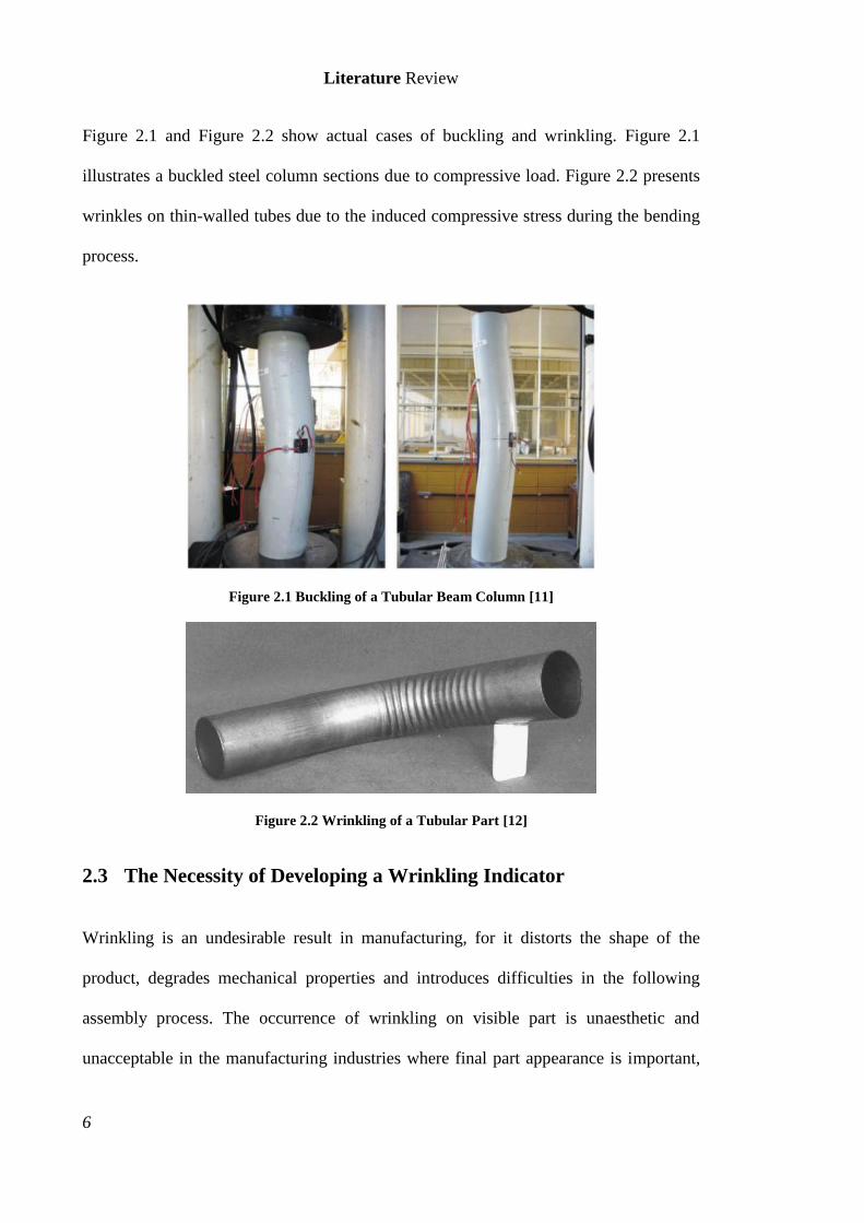
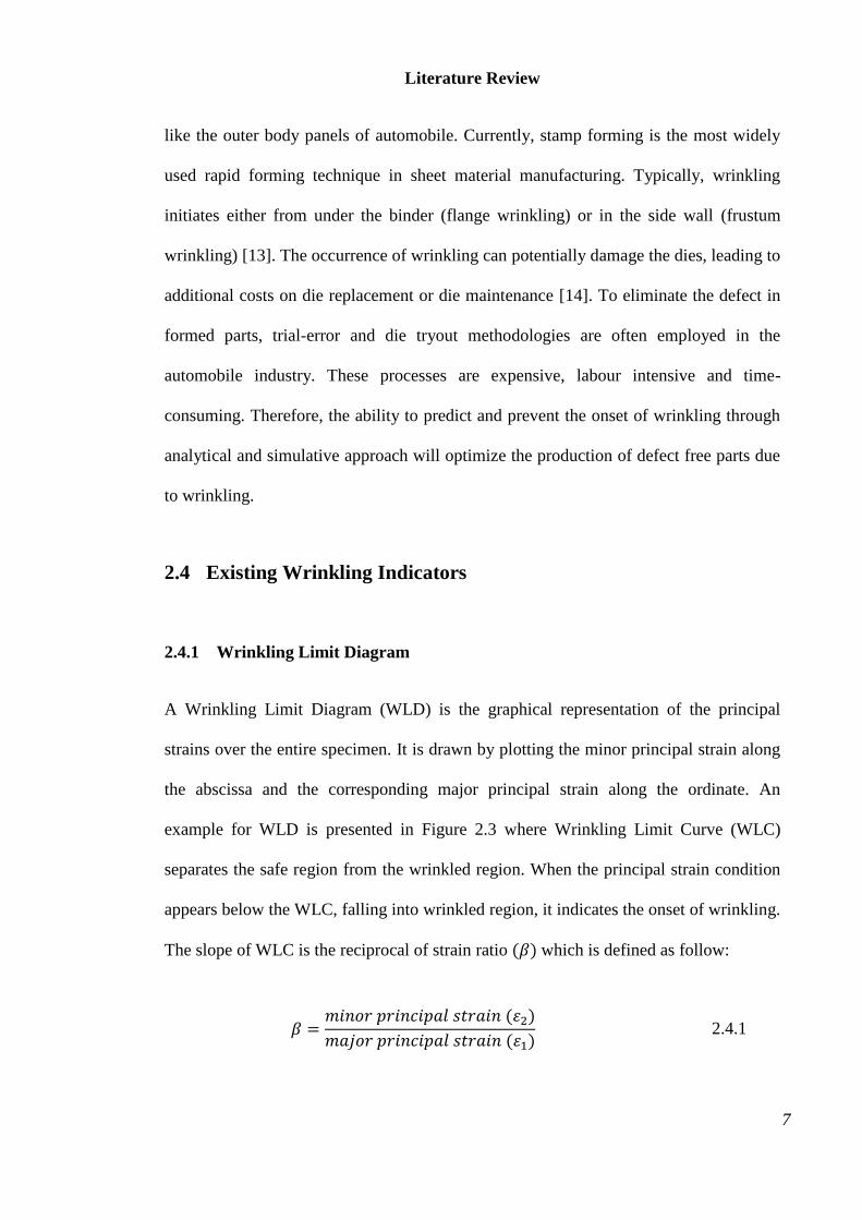
Figure 2.1 and Figure 2.2 show actual cases of buckling and wrinkling. Figure 2.1
illustrates a buckled steel column sections due to compressive load. Figure 2.2 presents
wrinkles on thin-walled tubes due to the induced compressive stress during the bending
process.
Figure 2.1 Buckling of a Tubular Beam Column [11]
Figure 2.2 Wrinkling of a Tubular Part [12]
2.3 The Necessity of Developing a Wrinkling Indicator
Wrinkling is an undesirable result in manufacturing, for it distorts the shape of the
product, degrades mechanical properties and introduces difficulties in the following
assembly process. The occurrence of wrinkling on visible part is unaesthetic and
unacceptable in the manufacturing industries where final part appearance is important,
Literature Review
7
like the outer body panels of automobile. Currently, stamp forming is the most widely
used rapid forming technique in sheet material manufacturing. Typically, wrinkling
initiates either from under the binder (flange wrinkling) or in the side wall (frustum
wrinkling) [13]. The occurrence of wrinkling can potentially damage the dies, leading to
additional costs on die replacement or die maintenance [14]. To eliminate the defect in
formed parts, trial-error and die tryout methodologies are often employed in the
automobile industry. These processes are expensive, labour intensive and time-
consuming. Therefore, the ability to predict and prevent the onset of wrinkling through
analytical and simulative approach will optimize the production of defect free parts due
to wrinkling.
2.4 Existing Wrinkling Indicators
2.4.1 Wrinkling Limit Diagram
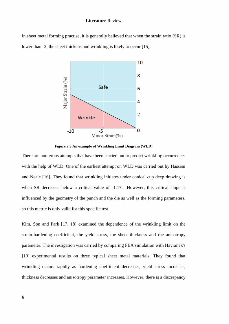
A Wrinkling Limit Diagram (WLD) is the graphical representation of the principal
strains over the entire specimen. It is drawn by plotting the minor principal strain along
the abscissa and the corresponding major principal strain along the ordinate. An
example for WLD is presented in Figure 2.3 where Wrinkling Limit Curve (WLC)
separates the safe region from the wrinkled region. When the principal strain condition
appears below the WLC, falling into wrinkled region, it indicates the onset of wrinkling.
The slope of WLC is the reciprocal of strain ratio (𝛽) which is defined as follow:
𝛽 =𝑚𝑖𝑛𝑜𝑟 𝑝𝑟𝑖𝑛𝑐𝑖𝑝𝑎𝑙 𝑠𝑡𝑟𝑎𝑖𝑛 (𝜀2)
𝑚𝑎𝑗𝑜𝑟 𝑝𝑟𝑖𝑛𝑐𝑖𝑝𝑎𝑙 𝑠𝑡𝑟𝑎𝑖𝑛 (𝜀1) 2.4.1
Literature Review
8
In sheet metal forming practise, it is generally believed that when the strain ratio (SR) is
lower than -2, the sheet thickens and wrinkling is likely to occur [15].
Figure 2.3 An example of Wrinkling Limit Diagram (WLD)
There are numerous attempts that have been carried out to predict wrinkling occurrences
with the help of WLD. One of the earliest attempt on WLD was carried out by Hassani
and Neale [16]. They found that wrinkling initiates under conical cup deep drawing is
when SR decreases below a critical value of -1.17. However, this critical slope is
influenced by the geometry of the punch and the die as well as the forming parameters,
so this metric is only valid for this specific test.
Kim, Son and Park [17, 18] examined the dependence of the wrinkling limit on the
strain-hardening coefficient, the yield stress, the sheet thickness and the anisotropy
parameter. The investigation was carried by comparing FEA simulation with Havranek's
[19] experimental results on three typical sheet metal materials. They found that
wrinkling occurs rapidly as hardening coefficient decreases, yield stress increases,
thickness decreases and anisotropy parameter increases. However, there is a discrepancy
Literature Review
9
between the numerical results and Havranek's experimental tests [19]. Experimental
results suggested that principal strain at critical condition (wrinkling limit) fall into a
narrow linear band regardless of the material thickness, while simulation results showed
that critical strain becomes larger as thickness increases. Their work focused only on
three types of metal materials in a particular type of conical cup forming so the outcome
may not be applicable to other class of material like composites and to other geometries.
Szacinski and Thomson [20] investigated the existence of a WLC by analysing strain
behaviour at the onset of wrinkling in a representative industrial sink bowl forming test.
Rectangular specimens made out of annealed 301 austenitic stainless-steel with a
constant thickness of 0.9 mm were formed to depths of 50 mm, 150 mm and 190 mm.
The gird marking technique facilitated the principal strain measurements from the final
wrinkled part by tracing movement of the vertices of the quadrilateral, drawn on the
initial un-deformed part. This methodology examined the localized strain condition in
the final product, but failed to provide information of strain evolution during the loading
process. The experimental results showed that wrinkling at the flange, corners of the
walls and mid-part of the walls appeared at different values of SR of approximately -1.0,
-0.5 and 0.5, respectively. Wrinkling limits are different at different regions on one part,
which makes the prediction of the onset of wrinkling by using WLD unpractical. They
pointed out that wrinkling might be indicated by the changes in strain path, but their
experimental methodology was unable to take a nuanced look of the strain evolvement
during the deformation process.
Narayanasamy et al. [21-24] evaluated the effect of mechanical properties on the
wrinkling initiation in conical and tractrix deep drawing. The sheet metal materials used
Literature Review
10
in these studies were commercially pure aluminium sheets annealed to different
annealing treatments [21, 24], aluminium 5086 alloy sheet annealed at different
temperatures [22] and interstitial-free steel sheet of different thickness [23]. They
examined the blanks with different diameters drawn through conical and tractrix die
using flat bottom punch. The grid measurements technique was employed for strain
measurement and the deformation of the grid on the formed part facilitated the
determination of localized strain distribution. To obtain a series of strain value before
and during wrinkling formation, the blanks were partially drawn to at least six different
depths until the wrinkling developed. The strain information obtained from each of the
partially drawn specimen provided the information for intermediate process. The
dependency of WLC was studied on these metal sheets for defining a safe working zone
for manufacturing application. The experimental results showed that higher Young's
modulus, higher yield stress, higher strain hardening value, higher anisotropy and larger
thickness exhibited better resistance against wrinkling.
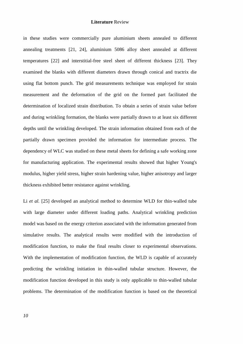
Li et al. [25] developed an analytical method to determine WLD for thin-walled tube
with large diameter under different loading paths. Analytical wrinkling prediction
model was based on the energy criterion associated with the information generated from
simulative results. The analytical results were modified with the introduction of
modification function, to make the final results closer to experimental observations.
With the implementation of modification function, the WLD is capable of accurately
predicting the wrinkling initiation in thin-walled tubular structure. However, the
modification function developed in this study is only applicable to thin-walled tubular
problems. The determination of the modification function is based on the theoretical
Literature Review
11
analysis of specimen geometries and boundary conditions, which make the employment
of this method to general forming operations difficult.
Djavanroodi and Derogar [26] numerically and experimentally evaluated WLD and
forming limit diagram (FLD) of hydroforming for Ti6Al4V titanium alloy and Al6061-
T6 aluminium alloy sheets. They used the existing theoretical fracture limit curves and
the SR of -2 for WLC to specify these two forms of failure in experimental and
simulative results. The strain measurement technique employed in experimental work
was the grid marking methodology, which only allows the strain information for the
initial and final stage. The experimental and simulative results suggested that the WLC,
with a SR of -2 can predict wrinkling phenomenon in this specific case. However, the
examination was only carried out at post-wrinkling step due to the limitation of the
strain measurement technique. There is no information available for the stage at or just
before the wrinkling initiation.
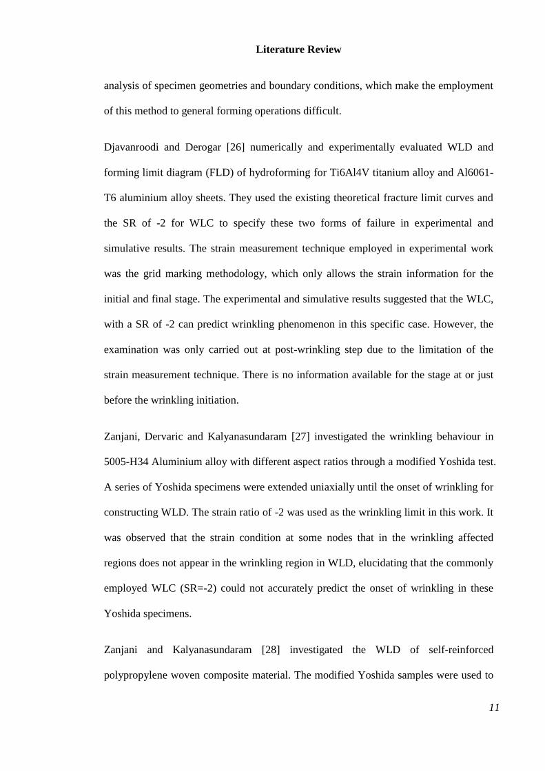
Zanjani, Dervaric and Kalyanasundaram [27] investigated the wrinkling behaviour in
5005-H34 Aluminium alloy with different aspect ratios through a modified Yoshida test.
A series of Yoshida specimens were extended uniaxially until the onset of wrinkling for
constructing WLD. The strain ratio of -2 was used as the wrinkling limit in this work. It
was observed that the strain condition at some nodes that in the wrinkling affected
regions does not appear in the wrinkling region in WLD, elucidating that the commonly
employed WLC (SR=-2) could not accurately predict the onset of wrinkling in these
Yoshida specimens.
Zanjani and Kalyanasundaram [28] investigated the WLD of self-reinforced
polypropylene woven composite material. The modified Yoshida samples were used to
Literature Review
12
study the onset of wrinkling in this work. To determine the wrinkling limit, the major
principal strain was plotted as a function of the minor principal strains for all surface
points at different elongation stages to construct WLD. It was reported that the initiation
of the wrinkling could be predicted under Yoshida test is when SR decreases below a
critical value. However, the critical SR for wrinkling limit was not given in this work,
because this value depends on the geometrical parameters and the material properties so
different test has a different critical value. The main contribution of this work was that it
checked the validity of WLD in the prediction of the wrinkling for composite materials.
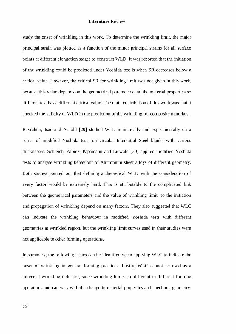
Bayraktar, Isac and Arnold [29] studied WLD numerically and experimentally on a
series of modified Yoshida tests on circular Interstitial Steel blanks with various
thicknesses. Schleich, Albiez, Papaioanu and Liewald [30] applied modified Yoshida
tests to analyse wrinkling behaviour of Aluminium sheet alloys of different geometry.
Both studies pointed out that defining a theoretical WLD with the consideration of
every factor would be extremely hard. This is attributable to the complicated link
between the geometrical parameters and the value of wrinkling limit, so the initiation
and propagation of wrinkling depend on many factors. They also suggested that WLC
can indicate the wrinkling behaviour in modified Yoshida tests with different
geometries at wrinkled region, but the wrinkling limit curves used in their studies were
not applicable to other forming operations.
In summary, the following issues can be identified when applying WLC to indicate the
onset of wrinkling in general forming practices. Firstly, WLC cannot be used as a
universal wrinkling indicator, since wrinkling limits are different in different forming
operations and can vary with the change in material properties and specimen geometry.
Literature Review
13
More importantly, there is a lack of indicator of the point of time when wrinkling starts
to occur. Most of current studies uses grid marking method to obtain the strain for
formed part. This method only gives the strain information at the final stage without
providing any information for the intermediate stages. Without adequate information
available for the stage corresponding to the onset of wrinkling, the current studies in the
literature lack the ability to predict the onset of wrinkling. Therefore, additional research
effort is required to find an indicator which can accurately predict the onset of wrinkling
for forming a wide range of production parts.
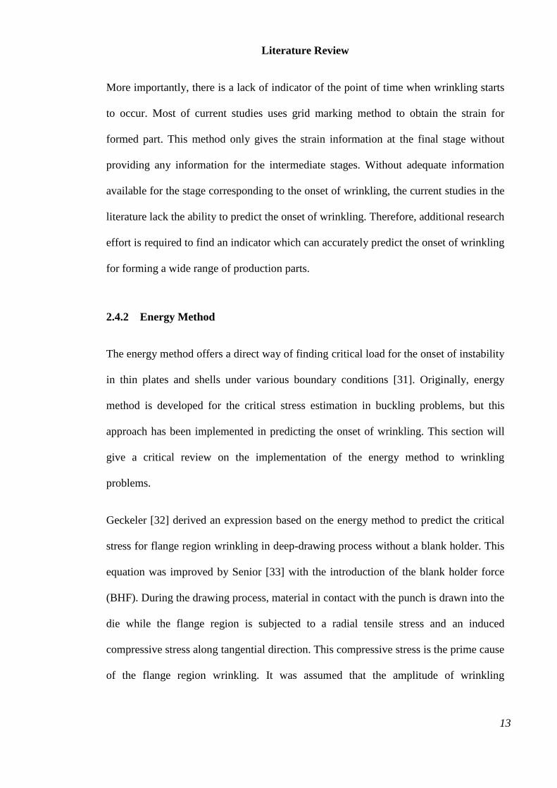
2.4.2 Energy Method
The energy method offers a direct way of finding critical load for the onset of instability
in thin plates and shells under various boundary conditions [31]. Originally, energy
method is developed for the critical stress estimation in buckling problems, but this
approach has been implemented in predicting the onset of wrinkling. This section will
give a critical review on the implementation of the energy method to wrinkling
problems.
Geckeler [32] derived an expression based on the energy method to predict the critical
stress for flange region wrinkling in deep-drawing process without a blank holder. This
equation was improved by Senior [33] with the introduction of the blank holder force
(BHF). During the drawing process, material in contact with the punch is drawn into the
die while the flange region is subjected to a radial tensile stress and an induced
compressive stress along tangential direction. This compressive stress is the prime cause
of the flange region wrinkling. It was assumed that the amplitude of wrinkling
Literature Review
14
deflection is constant over the width of the flange, which is described by a single sine
curve. A rectangular flange segment on flange region, which wrinkled into a half-wave
sine shape, was selected to represent the unit deflection of the flange region and to
simplify the usage of energy method. The critical stress for this segment can represent
the critical stress for the entire flange. The energy conservation theory states that the
critical condition is achieved when strain energy accumulated in the rectangular
segment equals to the work done by the external loading. For the wrinkling at flange
region, the sum of the bending energy and the restraining energy due to the lateral
constraint (blank holder effect) accumulated in the segment should equal to the work
done by the external loading calculated from the circumferential shortening of the
flange segment. Thus, the critical wrinkling stress for flange region can be determined.
It was reported that the overall flange deflection function including the number and the
amplitude of waves is crucial in the critical stress estimation, for it can affect the results
of estimated energy and in turn influence the expression of the critical stress for the
onset of wrinkling. For this reason, Senior [33] defined different surface deflection
function for different boundary conditions and material characteristics for critical stress
estimation.
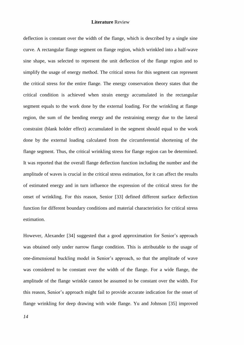
However, Alexander [34] suggested that a good approximation for Senior’s approach
was obtained only under narrow flange condition. This is attributable to the usage of
one-dimensional buckling model in Senior’s approach, so that the amplitude of wave
was considered to be constant over the width of the flange. For a wide flange, the
amplitude of the flange wrinkle cannot be assumed to be constant over the width. For
this reason, Senior’s approach might fail to provide accurate indication for the onset of
flange wrinkling for deep drawing with wide flange. Yu and Johnson [35] improved
Literature Review
15
Senior’s approach by improving the deflection function for the flange wrinkling. In this
study, the flange wrinkling under deep drawing process was simplified to an annular
plate simply supported at inner and outer edges, subjected to a radial tensile stress along
the inner edge to model the drawing effect and a normal constraint to simulate the
blank-holder effect. The deflection function of the annular plate was expressed in the
form of a two-dimensional buckling model. Zero deflection is defined along the inner
edge, while the deflection shape of the outer edge of the annular plate is expressed in
form of sine curve. The energy criterion with this modified deflection function was used
for the critical stress estimation. The main contribution of this work is that it gives
better definition of the deflection function for flange wrinkling under deep drawing
problems, compared to Senior’s approach.
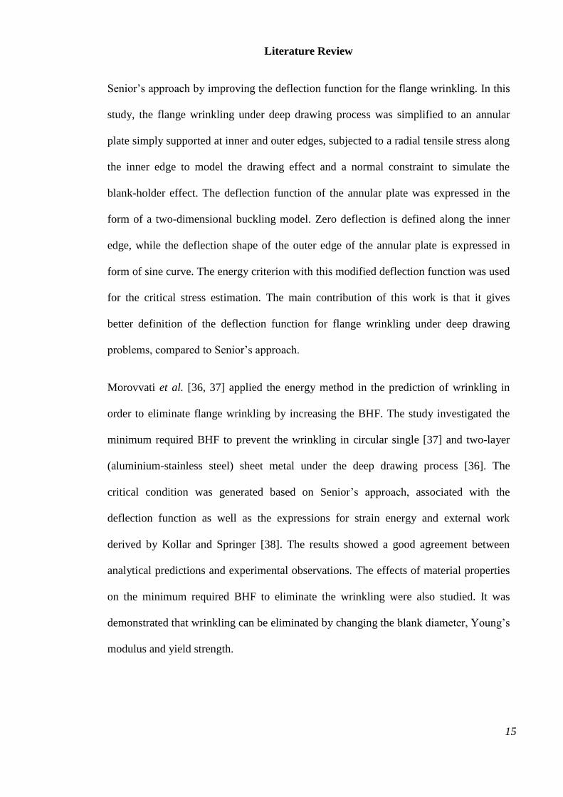
Morovvati et al. [36, 37] applied the energy method in the prediction of wrinkling in
order to eliminate flange wrinkling by increasing the BHF. The study investigated the
minimum required BHF to prevent the wrinkling in circular single [37] and two-layer
(aluminium-stainless steel) sheet metal under the deep drawing process [36]. The
critical condition was generated based on Senior’s approach, associated with the
deflection function as well as the expressions for strain energy and external work
derived by Kollar and Springer [38]. The results showed a good agreement between
analytical predictions and experimental observations. The effects of material properties
on the minimum required BHF to eliminate the wrinkling were also studied. It was
demonstrated that wrinkling can be eliminated by changing the blank diameter, Young’s
modulus and yield strength.

Literature Review
16
Agrawal, Reddy and Dixit [39, 40] investigated the minimum required BHF to achieve
wrinkle free parts with different thickness under deep drawing. Deep drawing process
was simplified to an annular plate simply supported at inner and outer edges. A radial
tensile stress imposed on the inner edge and a normal constraint was applied over the
surface to model the blank holder constraint. The deflection function of the annular
plate was set to zero at the inner edge and expressed in sine curve along the outer edge.
Then, the strain energy stored in the system, restraining energy of the blank holder and
the work done by external loadings were calculated for the critical wrinkling stress
estimation. The critical condition for the onset of wrinkling was determined by equating
the sum of strain energy and restraining energy to the work done by external loadings.
The predicted critical condition for the instability was validated with the published
experimental results [33, 35, 41] and good agreement was observed. The study showed
that a thicker specimen requires a higher BHF to eliminate the wrinkling.
Zheng et al. [42] carried out a series of deep drawing experiments on commercial
AA6082-T6 aluminium alloy sheet with a thickness of 1.5mm to test the effect of draw
ratios and blank-holding forces on the occurrence of flange wrinkling. The effect of
draw ratio, which is defined as the diameter of the blank (170, 180 and 190mm) over
the diameter of the punch (100mm), is also investigated. To examine the effects of
process parameters on the onset of wrinkling, analytical models based on energy
method were utilised in deep drawing of aluminium alloy. Bending energy, restraining
energy and the work done by the external loading is estimated for a representative
segment. This segment is selected from the flange region and assumed to have a half-
wave sine shape. The critical wrinkling condition is achieved when the sum of bending
and restraining energy equals to the external work. Two buckling modes (one-
Literature Review
17
dimensional and two-dimensional buckling mode) were examined for the estimation of
the critical wrinkling condition for the flange region and the flange segment. The
comparison with the experimental observations suggested that the model employing the
two-dimensional buckling mode exhibits a better agreement than the one implementing
with the one-dimensional deflection function. Both analytical and experimental results
illustrated that draw ratio had a significant effect on the onset of wrinkling but the
blank-holding force did not. Wrinkling is easier to initiate at a larger draw ratio (bigger
blank).
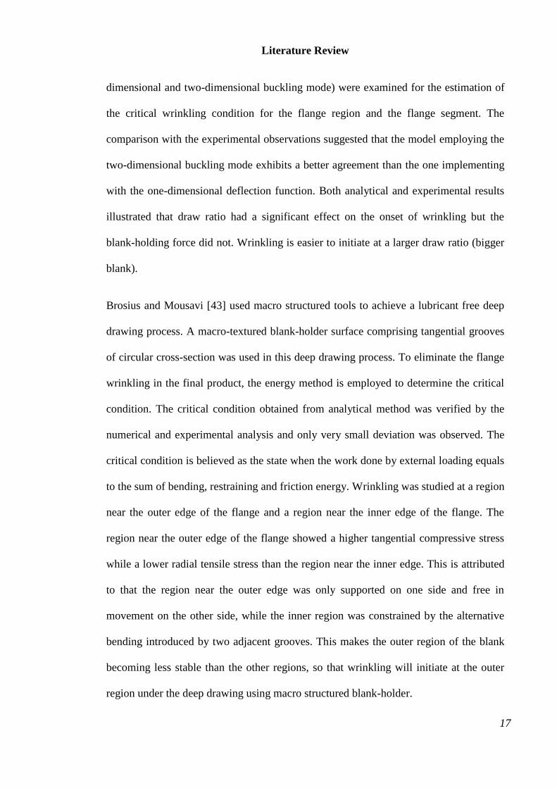
Brosius and Mousavi [43] used macro structured tools to achieve a lubricant free deep
drawing process. A macro-textured blank-holder surface comprising tangential grooves
of circular cross-section was used in this deep drawing process. To eliminate the flange
wrinkling in the final product, the energy method is employed to determine the critical
condition. The critical condition obtained from analytical method was verified by the
numerical and experimental analysis and only very small deviation was observed. The
critical condition is believed as the state when the work done by external loading equals
to the sum of bending, restraining and friction energy. Wrinkling was studied at a region
near the outer edge of the flange and a region near the inner edge of the flange. The
region near the outer edge of the flange showed a higher tangential compressive stress
while a lower radial tensile stress than the region near the inner edge. This is attributed
to that the region near the outer edge was only supported on one side and free in
movement on the other side, while the inner region was constrained by the alternative
bending introduced by two adjacent grooves. This makes the outer region of the blank
becoming less stable than the other regions, so that wrinkling will initiate at the outer
region under the deep drawing using macro structured blank-holder.
Literature Review
18
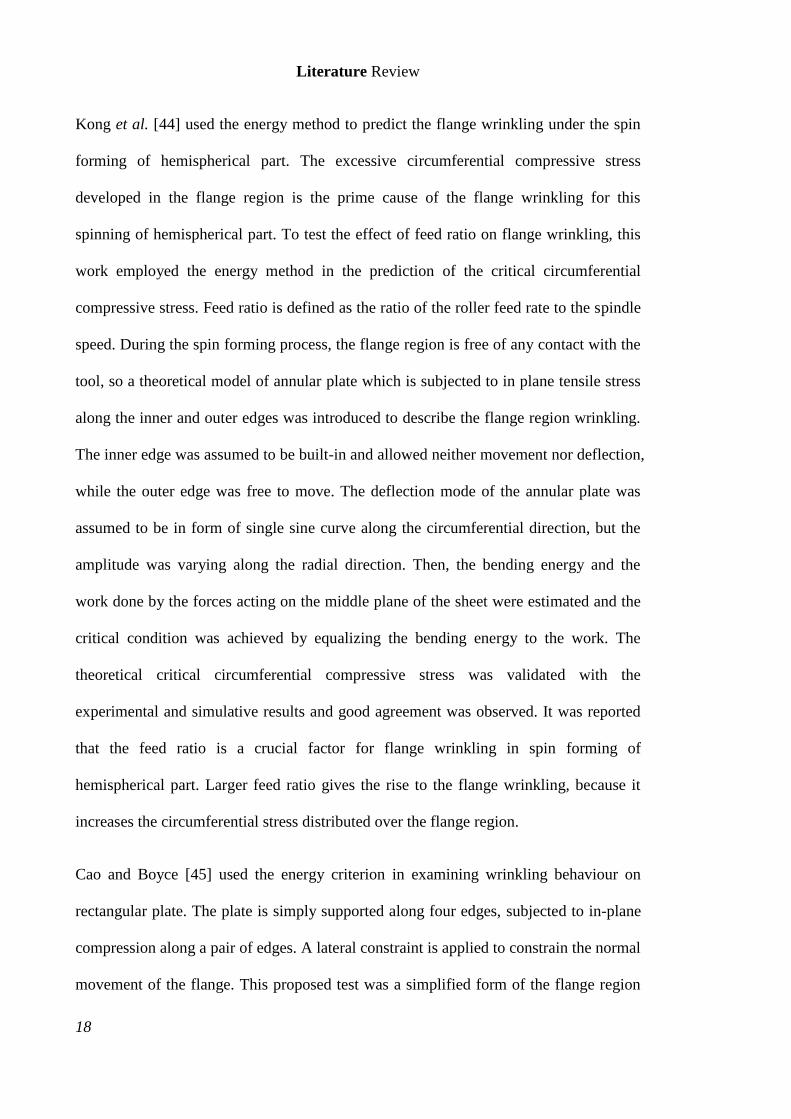
Kong et al. [44] used the energy method to predict the flange wrinkling under the spin
forming of hemispherical part. The excessive circumferential compressive stress
developed in the flange region is the prime cause of the flange wrinkling for this
spinning of hemispherical part. To test the effect of feed ratio on flange wrinkling, this
work employed the energy method in the prediction of the critical circumferential
compressive stress. Feed ratio is defined as the ratio of the roller feed rate to the spindle
speed. During the spin forming process, the flange region is free of any contact with the
tool, so a theoretical model of annular plate which is subjected to in plane tensile stress
along the inner and outer edges was introduced to describe the flange region wrinkling.
The inner edge was assumed to be built-in and allowed neither movement nor deflection,
while the outer edge was free to move. The deflection mode of the annular plate was
assumed to be in form of single sine curve along the circumferential direction, but the
amplitude was varying along the radial direction. Then, the bending energy and the
work done by the forces acting on the middle plane of the sheet were estimated and the
critical condition was achieved by equalizing the bending energy to the work. The
theoretical critical circumferential compressive stress was validated with the
experimental and simulative results and good agreement was observed. It was reported
that the feed ratio is a crucial factor for flange wrinkling in spin forming of
hemispherical part. Larger feed ratio gives the rise to the flange wrinkling, because it
increases the circumferential stress distributed over the flange region.
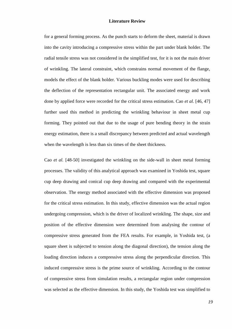
Cao and Boyce [45] used the energy criterion in examining wrinkling behaviour on
rectangular plate. The plate is simply supported along four edges, subjected to in-plane
compression along a pair of edges. A lateral constraint is applied to constrain the normal
movement of the flange. This proposed test was a simplified form of the flange region
Literature Review
19
for a general forming process. As the punch starts to deform the sheet, material is drawn
into the cavity introducing a compressive stress within the part under blank holder. The
radial tensile stress was not considered in the simplified test, for it is not the main driver
of wrinkling. The lateral constraint, which constrains normal movement of the flange,
models the effect of the blank holder. Various buckling modes were used for describing
the deflection of the representation rectangular unit. The associated energy and work
done by applied force were recorded for the critical stress estimation. Cao et al. [46, 47]
further used this method in predicting the wrinkling behaviour in sheet metal cup
forming. They pointed out that due to the usage of pure bending theory in the strain
energy estimation, there is a small discrepancy between predicted and actual wavelength
when the wavelength is less than six times of the sheet thickness.
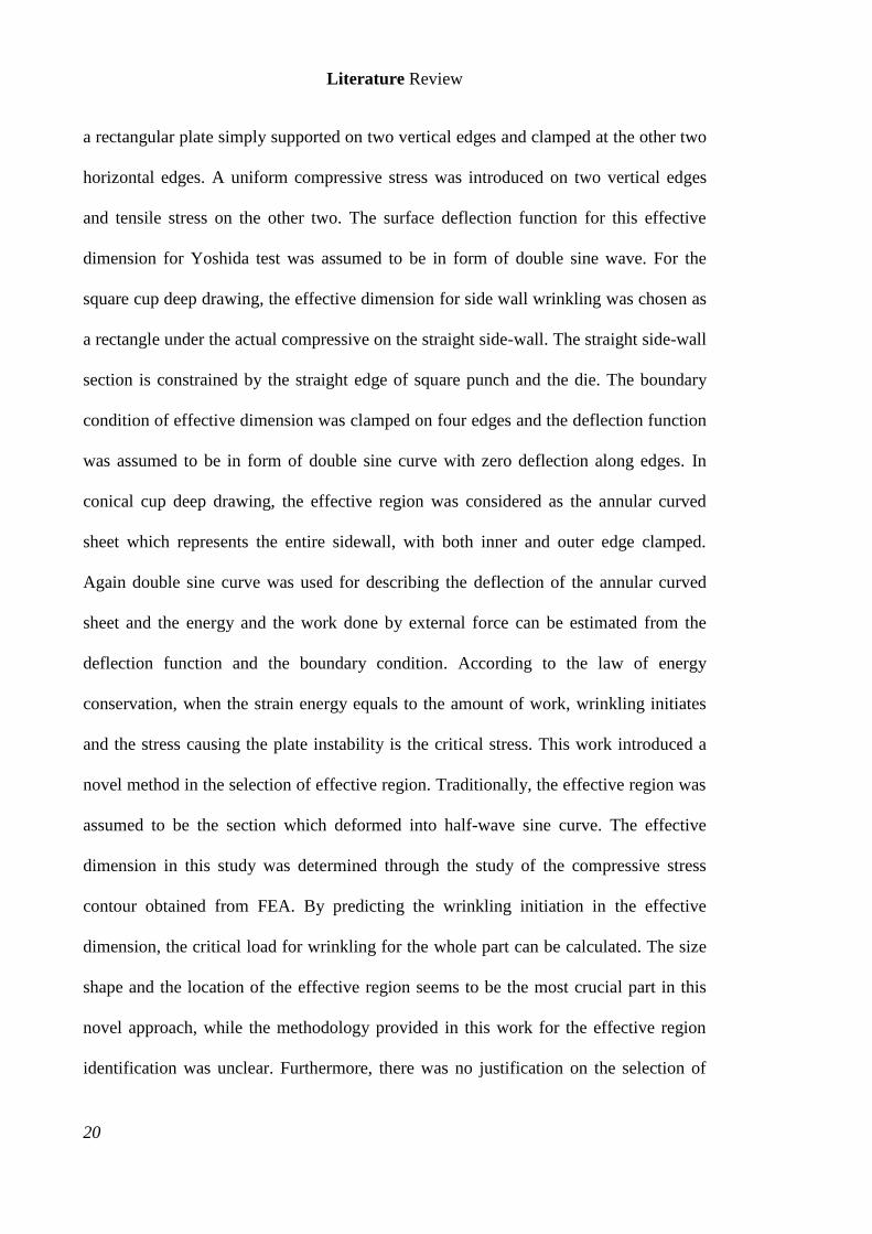
Cao et al. [48-50] investigated the wrinkling on the side-wall in sheet metal forming
processes. The validity of this analytical approach was examined in Yoshida test, square
cup deep drawing and conical cup deep drawing and compared with the experimental
observation. The energy method associated with the effective dimension was proposed
for the critical stress estimation. In this study, effective dimension was the actual region
undergoing compression, which is the driver of localized wrinkling. The shape, size and
position of the effective dimension were determined from analysing the contour of
compressive stress generated from the FEA results. For example, in Yoshida test, (a
square sheet is subjected to tension along the diagonal direction), the tension along the
loading direction induces a compressive stress along the perpendicular direction. This
induced compressive stress is the prime source of wrinkling. According to the contour
of compressive stress from simulation results, a rectangular region under compression
was selected as the effective dimension. In this study, the Yoshida test was simplified to
Literature Review
20
a rectangular plate simply supported on two vertical edges and clamped at the other two
horizontal edges. A uniform compressive stress was introduced on two vertical edges
and tensile stress on the other two. The surface deflection function for this effective
dimension for Yoshida test was assumed to be in form of double sine wave. For the
square cup deep drawing, the effective dimension for side wall wrinkling was chosen as
a rectangle under the actual compressive on the straight side-wall. The straight side-wall
section is constrained by the straight edge of square punch and the die. The boundary
condition of effective dimension was clamped on four edges and the deflection function
was assumed to be in form of double sine curve with zero deflection along edges. In
conical cup deep drawing, the effective region was considered as the annular curved
sheet which represents the entire sidewall, with both inner and outer edge clamped.
Again double sine curve was used for describing the deflection of the annular curved
sheet and the energy and the work done by external force can be estimated from the
deflection function and the boundary condition. According to the law of energy
conservation, when the strain energy equals to the amount of work, wrinkling initiates
and the stress causing the plate instability is the critical stress. This work introduced a
novel method in the selection of effective region. Traditionally, the effective region was
assumed to be the section which deformed into half-wave sine curve. The effective
dimension in this study was determined through the study of the compressive stress
contour obtained from FEA. By predicting the wrinkling initiation in the effective
dimension, the critical load for wrinkling for the whole part can be calculated. The size
shape and the location of the effective region seems to be the most crucial part in this
novel approach, while the methodology provided in this work for the effective region
identification was unclear. Furthermore, there was no justification on the selection of
Literature Review
21
the boundary conditions on the effective region, so that it seems to be challenge to apply
this novel methodology to other cases.
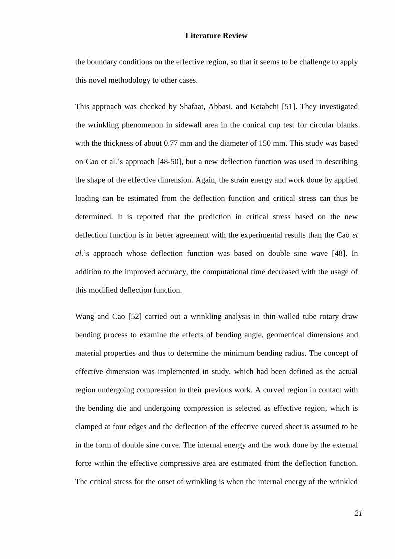
This approach was checked by Shafaat, Abbasi, and Ketabchi [51]. They investigated
the wrinkling phenomenon in sidewall area in the conical cup test for circular blanks
with the thickness of about 0.77 mm and the diameter of 150 mm. This study was based
on Cao et al.’s approach [48-50], but a new deflection function was used in describing
the shape of the effective dimension. Again, the strain energy and work done by applied
loading can be estimated from the deflection function and critical stress can thus be
determined. It is reported that the prediction in critical stress based on the new
deflection function is in better agreement with the experimental results than the Cao et
al.’s approach whose deflection function was based on double sine wave [48]. In
addition to the improved accuracy, the computational time decreased with the usage of
this modified deflection function.
Wang and Cao [52] carried out a wrinkling analysis in thin-walled tube rotary draw
bending process to examine the effects of bending angle, geometrical dimensions and
material properties and thus to determine the minimum bending radius. The concept of
effective dimension was implemented in study, which had been defined as the actual
region undergoing compression in their previous work. A curved region in contact with
the bending die and undergoing compression is selected as effective region, which is
clamped at four edges and the deflection of the effective curved sheet is assumed to be
in the form of double sine curve. The internal energy and the work done by the external
force within the effective compressive area are estimated from the deflection function.
The critical stress for the onset of wrinkling is when the internal energy of the wrinkled
Literature Review
22
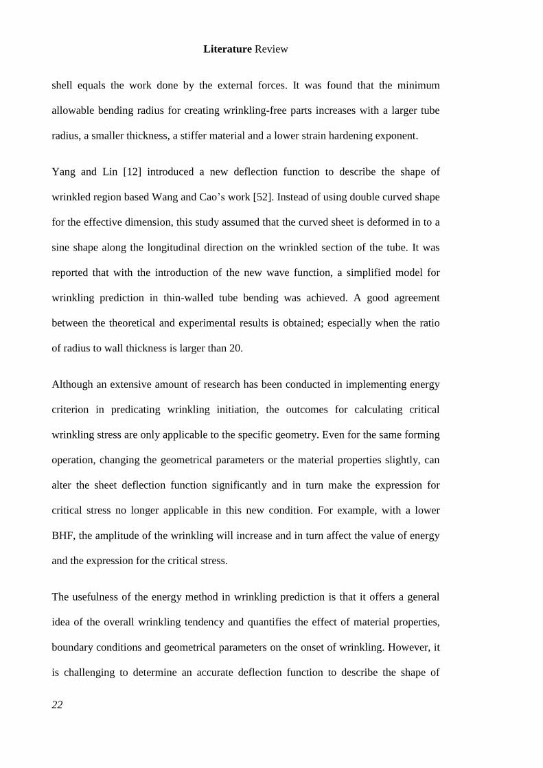
shell equals the work done by the external forces. It was found that the minimum
allowable bending radius for creating wrinkling-free parts increases with a larger tube
radius, a smaller thickness, a stiffer material and a lower strain hardening exponent.
Yang and Lin [12] introduced a new deflection function to describe the shape of
wrinkled region based Wang and Cao’s work [52]. Instead of using double curved shape
for the effective dimension, this study assumed that the curved sheet is deformed in to a
sine shape along the longitudinal direction on the wrinkled section of the tube. It was
reported that with the introduction of the new wave function, a simplified model for
wrinkling prediction in thin-walled tube bending was achieved. A good agreement
between the theoretical and experimental results is obtained; especially when the ratio
of radius to wall thickness is larger than 20.
Although an extensive amount of research has been conducted in implementing energy
criterion in predicating wrinkling initiation, the outcomes for calculating critical
wrinkling stress are only applicable to the specific geometry. Even for the same forming
operation, changing the geometrical parameters or the material properties slightly, can
alter the sheet deflection function significantly and in turn make the expression for
critical stress no longer applicable in this new condition. For example, with a lower
BHF, the amplitude of the wrinkling will increase and in turn affect the value of energy
and the expression for the critical stress.
The usefulness of the energy method in wrinkling prediction is that it offers a general
idea of the overall wrinkling tendency and quantifies the effect of material properties,
boundary conditions and geometrical parameters on the onset of wrinkling. However, it
is challenging to determine an accurate deflection function to describe the shape of
Literature Review
23
wrinkling and energy method is developed based on several assumptions, such as the
thickness is uniform over the sheet; the stress through the thickness is uniform before
wrinkling. For this reason, a discrepancy may occur between the theoretical predicted
results and actual experiment observation.
2.5 Summary
This chapter summarizes literatures related to wrinkling. Firstly, a comparison between
wrinkling and buckling phenomenon is presented. Then, this chapter highlights the need
of a reliable and robust wrinkling indicator. Finally, a critical and extensive review on
the existing wrinkling indicators is given, including wrinkling limit diagram (WLD) and
analytical energy methods.
It is concluded that while an extensive amount of research has been done on the
wrinkling prediction, there is no mature wrinkling indicator for the onset of wrinkling.
WLC is the most intensively used one. Though several studies suggested that it is viable
for complex forming operations, the wrinkling limit had to be determined case by case.
The fundamental difficulty with WLC is that it can be different for different geometries
and furthermore it can be different for different locations of the same part. It also fails to
provide a clear indication of the exact point of time when the sheet first to wrinkle for
localized wrinkled region. On the other hand the analytical approach gives the exact
value of critical load and a clear relationship between the onset of wrinkling and the
effective parameters. However, comparing with WLD, it is more difficult for energy
approach to solve problems with complicated boundary conditions and irregular
geometrical shapes.

Literature Review
24
This literature indicates that whilst considerable research has been carried out on
wrinkling problems, a robust indicator that can be applied to a wide range production
parts does not exist and will be the focus of this study.
Materials and Methodology
25
Chapter 3 Materials and Methodology
3.1 Introduction
An overview of composite material and the manufacturing techniques of two woven
thermoplastic composite materials studied in this thesis are firstly given. This is
followed by an introduction of the experimental methodology of using the Yoshida test,
including the experimental set up and specimen preparation. Finally, the details of FEA
modelling are presented.
3.2 Woven Thermoplastic Composites
Fibre reinforced composite materials consist of high strength fibre reinforcement to
carry the load and a matrix to transfer the load between fibres [53-56]. Normally, the
woven composite material will exhibit better damage resistance than unwoven
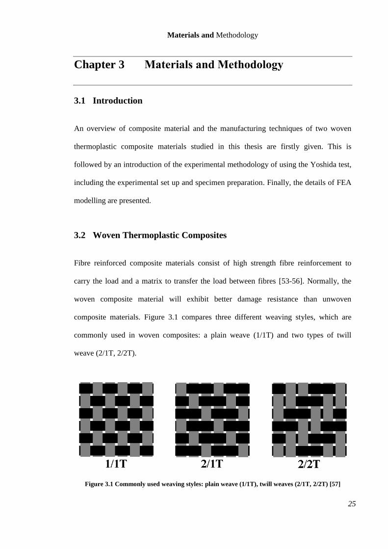
composite materials. Figure 3.1 compares three different weaving styles, which are
commonly used in woven composites: a plain weave (1/1T) and two types of twill
weave (2/1T, 2/2T).
Figure 3.1 Commonly used weaving styles: plain weave (1/1T), twill weaves (2/1T, 2/2T) [57]
Materials and Methodology
26
In a plain weave, each warp fibre passes alternately under and over each weft fibre,
leading to a balanced structure. In a twill weave, each weft yarn floats across two or
more warp yarn in a regular repeated manner. The balanced woven structure, such as the
plain weave, 2/2 twill, 3/3 twill weave, minimizes the occurrence and the magnitude of
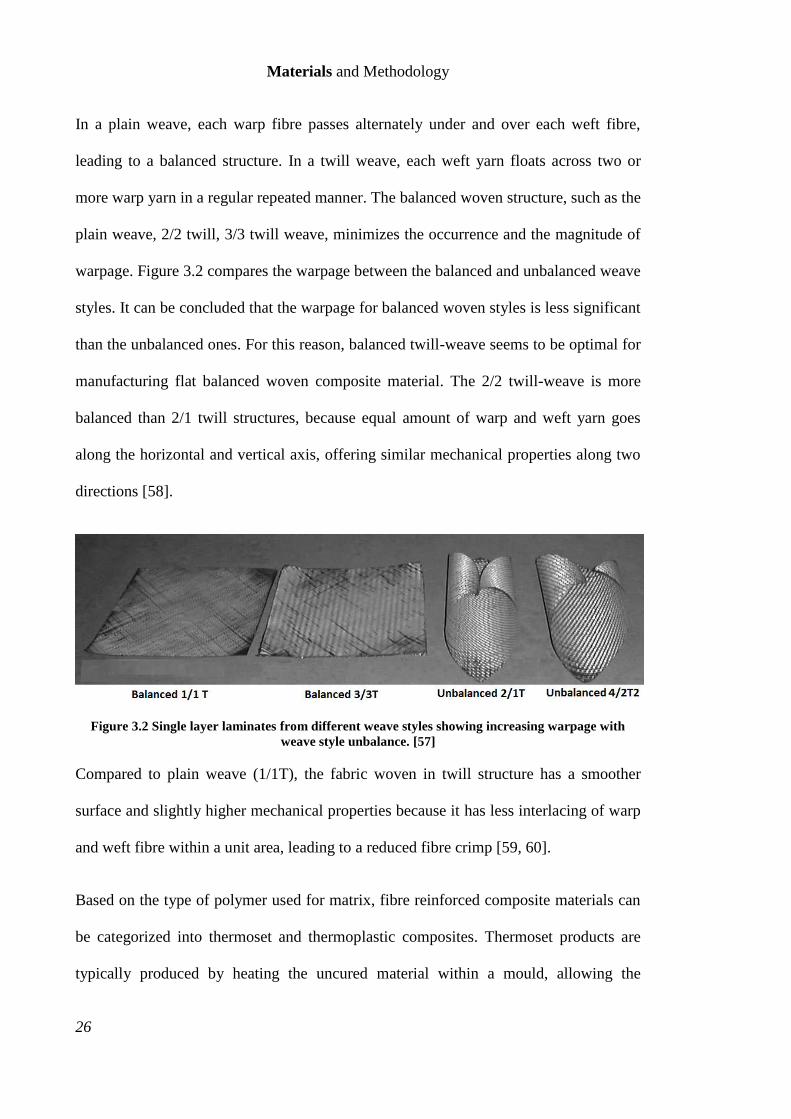
warpage. Figure 3.2 compares the warpage between the balanced and unbalanced weave
styles. It can be concluded that the warpage for balanced woven styles is less significant
than the unbalanced ones. For this reason, balanced twill-weave seems to be optimal for
manufacturing flat balanced woven composite material. The 2/2 twill-weave is more
balanced than 2/1 twill structures, because equal amount of warp and weft yarn goes
along the horizontal and vertical axis, offering similar mechanical properties along two
directions [58].
Figure 3.2 Single layer laminates from different weave styles showing increasing warpage with
weave style unbalance. [57]
Compared to plain weave (1/1T), the fabric woven in twill structure has a smoother
surface and slightly higher mechanical properties because it has less interlacing of warp
and weft fibre within a unit area, leading to a reduced fibre crimp [59, 60].
Based on the type of polymer used for matrix, fibre reinforced composite materials can
be categorized into thermoset and thermoplastic composites. Thermoset products are
typically produced by heating the uncured material within a mould, allowing the
Materials and Methodology
27
material to cure into its final shape [61, 62]. Due to the nature of the irreversible cross-
linking of polymer chains during curing process, thermoset composites cannot be
remoulded or reshaped and they are very difficult to recycle. However, this process
introduces a highly linked three-dimensional molecular network offering thermoset
matrices a better temperature resistance than thermoplastic composite material [63].
Thermoplastic composite material can be moulded, melted and remoulded without
altering the chemical component, so they are easier to repair and recycle compared to
thermoset composites [64, 65]. The majority of thermoplastic materials will not
withstand a temperature of over 100°C over an extended period and only a few will
withstand temperatures above 350°C [66]. For example, the melting temperature for
commercial isotactic polypropylene (PP) ranges from 160 to 166 °C [67]; poly-ether-
ether-ketone (PEEK) melts at around 340 °C [68]. Generally thermoplastic matrix
composite materials are tougher and more ductile than thermosets, providing better
impact resistance and damage tolerance. They are less dense than thermosets, making
them an alternative for weight critical applications. Two different woven thermoplastic
composite materials are used in the study (Curv® and Twintex®).
3.2.1 Curv®
Curv® is a self-reinforced polypropylene composite material with a fibre volume
fraction of 55-65 percent [69]. The same polymer forms both the reinforcement and
matrix phase, exhibiting a better recycling option compared to other thermoplastic
composite materials which have two different materials for matrix and fiber [70]. In
addition to the elevated recyclability, the weight of lightweight parts can be further
Materials and Methodology
28
reduced compared to the conventional fiber reinforced thermoplastic composites. The
density of polypropylene reinforcement is 0.9g/cm3, which is much lower than that of
glass (2.5-2.9g/cm3), carbon (1.7-1.9g/cm
3) and basalt (2.7-3.0g/cm
3) [71, 72]. For
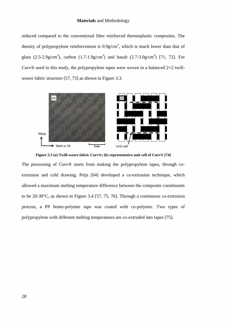
Curv® used in this study, the polypropylene tapes were woven in a balanced 2×2 twill-
weave fabric structure [57, 73] as shown in Figure 3.3.
Figure 3.3 (a) Twill-weave fabric Curv®; (b) representative unit cell of Curv® [74]
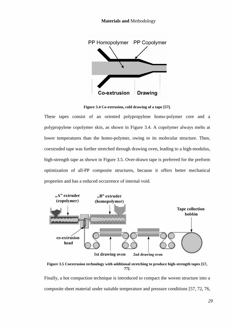
The processing of Curv® starts from making the polypropylene tapes, through co-
extrusion and cold drawing. Peijs [64] developed a co-extrusion technique, which
allowed a maximum melting temperature difference between the composite constituents
to be 20-30°C, as shown in Figure 3.4 [57, 75, 76]. Through a continuous co-extrusion
process, a PP homo-polymer tape was coated with co-polymer. Two types of
polypropylene with different melting temperatures are co-extruded into tapes [75].
Materials and Methodology
29
Figure 3.4 Co-extrusion, cold drawing of a tape [57].
These tapes consist of an oriented polypropylene homo-polymer core and a
polypropylene copolymer skin, as shown in Figure 3.4. A copolymer always melts at
lower temperatures than the homo-polymer, owing to its molecular structure. Then,
coextruded tape was further stretched through drawing oven, leading to a high-modulus,
high-strength tape as shown in Figure 3.5. Over-drawn tape is preferred for the preform
optimization of all-PP composite structures, because it offers better mechanical
properties and has a reduced occurrence of internal void.
Figure 3.5 Coextrusion technology with additional stretching to produce high-strength tapes [57,
77].
Finally, a hot compaction technique is introduced to compact the woven structure into a
composite sheet material under suitable temperature and pressure conditions [57, 72, 76,
Materials and Methodology
30
78, 79]. The fabric is subjected to a specific pressure depending on the thickness to
prevent the thermal shrinkage. Typically, the compaction temperature is controlled
between 140°C and 190°C [57, 72] and the temperature and pressure are kept for around
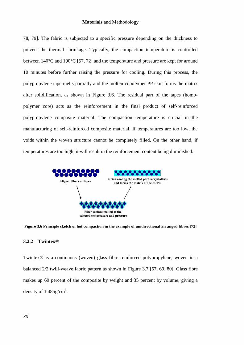
10 minutes before further raising the pressure for cooling. During this process, the
polypropylene tape melts partially and the molten copolymer PP skin forms the matrix
after solidification, as shown in Figure 3.6. The residual part of the tapes (homo-
polymer core) acts as the reinforcement in the final product of self-reinforced
polypropylene composite material. The compaction temperature is crucial in the
manufacturing of self-reinforced composite material. If temperatures are too low, the
voids within the woven structure cannot be completely filled. On the other hand, if
temperatures are too high, it will result in the reinforcement content being diminished.
Figure 3.6 Principle sketch of hot compaction in the example of unidirectional arranged fibres [72]
3.2.2 Twintex®
Twintex® is a continuous (woven) glass fibre reinforced polypropylene, woven in a
balanced 2/2 twill-weave fabric pattern as shown in Figure 3.7 [57, 69, 80]. Glass fibre
makes up 60 percent of the composite by weight and 35 percent by volume, giving a
density of 1.485g/cm3.
Materials and Methodology
31
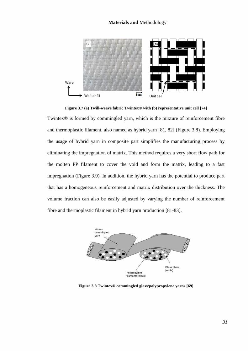
Figure 3.7 (a) Twill-weave fabric Twintex® with (b) representative unit cell [74]
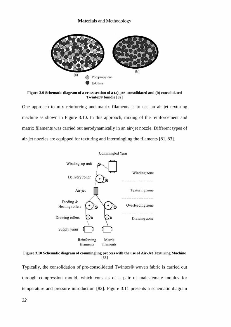
Twintex® is formed by commingled yarn, which is the mixture of reinforcement fibre
and thermoplastic filament, also named as hybrid yarn [81, 82] (Figure 3.8). Employing
the usage of hybrid yarn in composite part simplifies the manufacturing process by
eliminating the impregnation of matrix. This method requires a very short flow path for
the molten PP filament to cover the void and form the matrix, leading to a fast
impregnation (Figure 3.9). In addition, the hybrid yarn has the potential to produce part
that has a homogeneous reinforcement and matrix distribution over the thickness. The
volume fraction can also be easily adjusted by varying the number of reinforcement
fibre and thermoplastic filament in hybrid yarn production [81-83].
Figure 3.8 Twintex® commingled glass/polypropylene yarns [69]
Materials and Methodology
32
Figure 3.9 Schematic diagram of a cross section of a (a) pre-consolidated and (b) consolidated
Twintex® bundle [82]
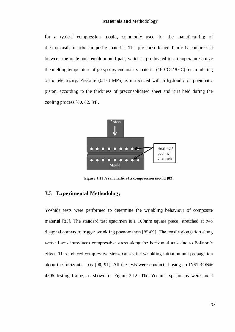
One approach to mix reinforcing and matrix filaments is to use an air-jet texturing
machine as shown in Figure 3.10. In this approach, mixing of the reinforcement and
matrix filaments was carried out aerodynamically in an air-jet nozzle. Different types of
air-jet nozzles are equipped for texturing and intermingling the filaments [81, 83].
Figure 3.10 Schematic diagram of commingling process with the use of Air-Jet Texturing Machine
[83]
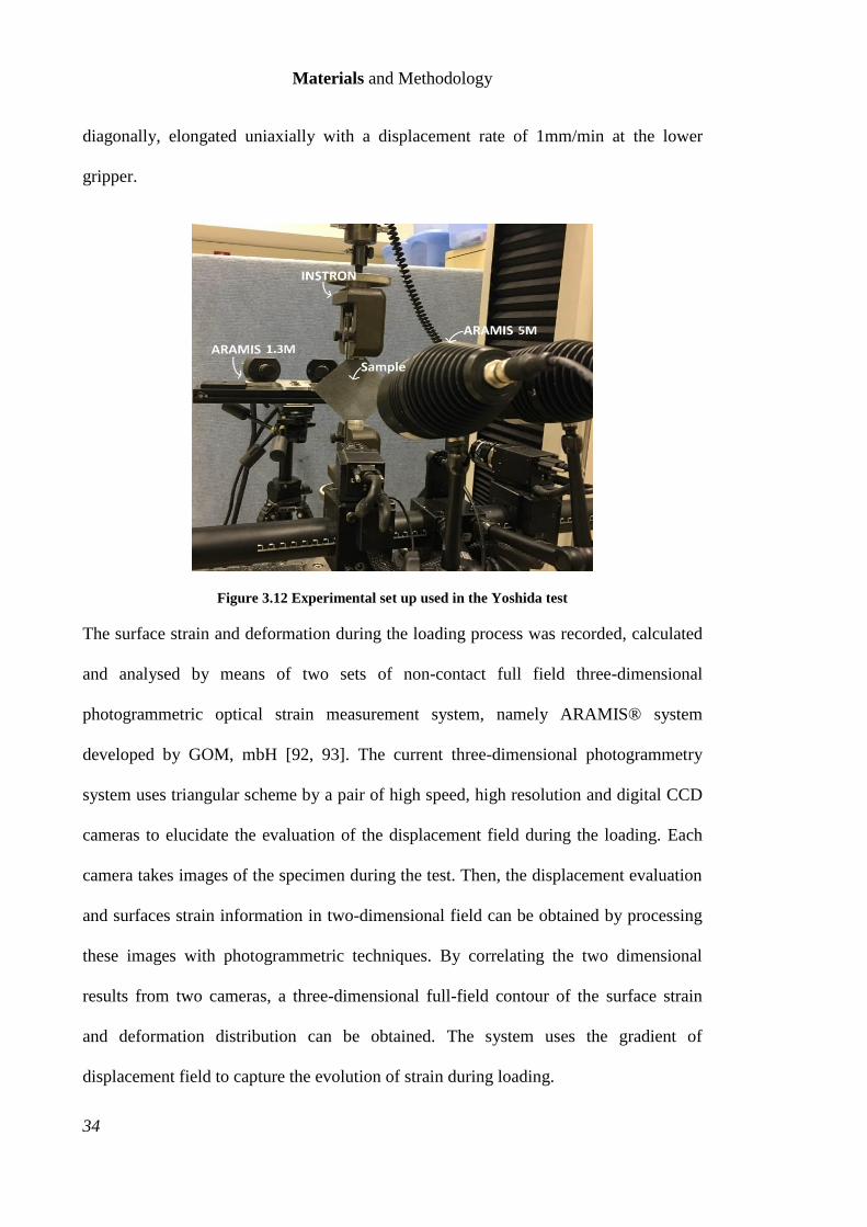
Typically, the consolidation of pre-consolidated Twintex® woven fabric is carried out
through compression mould, which consists of a pair of male-female moulds for
temperature and pressure introduction [82]. Figure 3.11 presents a schematic diagram
Materials and Methodology
33
for a typical compression mould, commonly used for the manufacturing of
thermoplastic matrix composite material. The pre-consolidated fabric is compressed
between the male and female mould pair, which is pre-heated to a temperature above
the melting temperature of polypropylene matrix material (180°C-230°C) by circulating
oil or electricity. Pressure (0.1-3 MPa) is introduced with a hydraulic or pneumatic
piston, according to the thickness of preconsolidated sheet and it is held during the
cooling process [80, 82, 84].
Figure 3.11 A schematic of a compression mould [82]
3.3 Experimental Methodology
Yoshida tests were performed to determine the wrinkling behaviour of composite
material [85]. The standard test specimen is a 100mm square piece, stretched at two
diagonal corners to trigger wrinkling phenomenon [85-89]. The tensile elongation along
vertical axis introduces compressive stress along the horizontal axis due to Poisson’s
effect. This induced compressive stress causes the wrinkling initiation and propagation
along the horizontal axis [90, 91]. All the tests were conducted using an INSTRON®
4505 testing frame, as shown in Figure 3.12. The Yoshida specimens were fixed
Materials and Methodology
34
diagonally, elongated uniaxially with a displacement rate of 1mm/min at the lower
gripper.
Figure 3.12 Experimental set up used in the Yoshida test
The surface strain and deformation during the loading process was recorded, calculated
and analysed by means of two sets of non-contact full field three-dimensional
photogrammetric optical strain measurement system, namely ARAMIS® system
developed by GOM, mbH [92, 93]. The current three-dimensional photogrammetry
system uses triangular scheme by a pair of high speed, high resolution and digital CCD
cameras to elucidate the evaluation of the displacement field during the loading. Each
camera takes images of the specimen during the test. Then, the displacement evaluation
and surfaces strain information in two-dimensional field can be obtained by processing
these images with photogrammetric techniques. By correlating the two dimensional
results from two cameras, a three-dimensional full-field contour of the surface strain
and deformation distribution can be obtained. The system uses the gradient of
displacement field to capture the evolution of strain during loading.
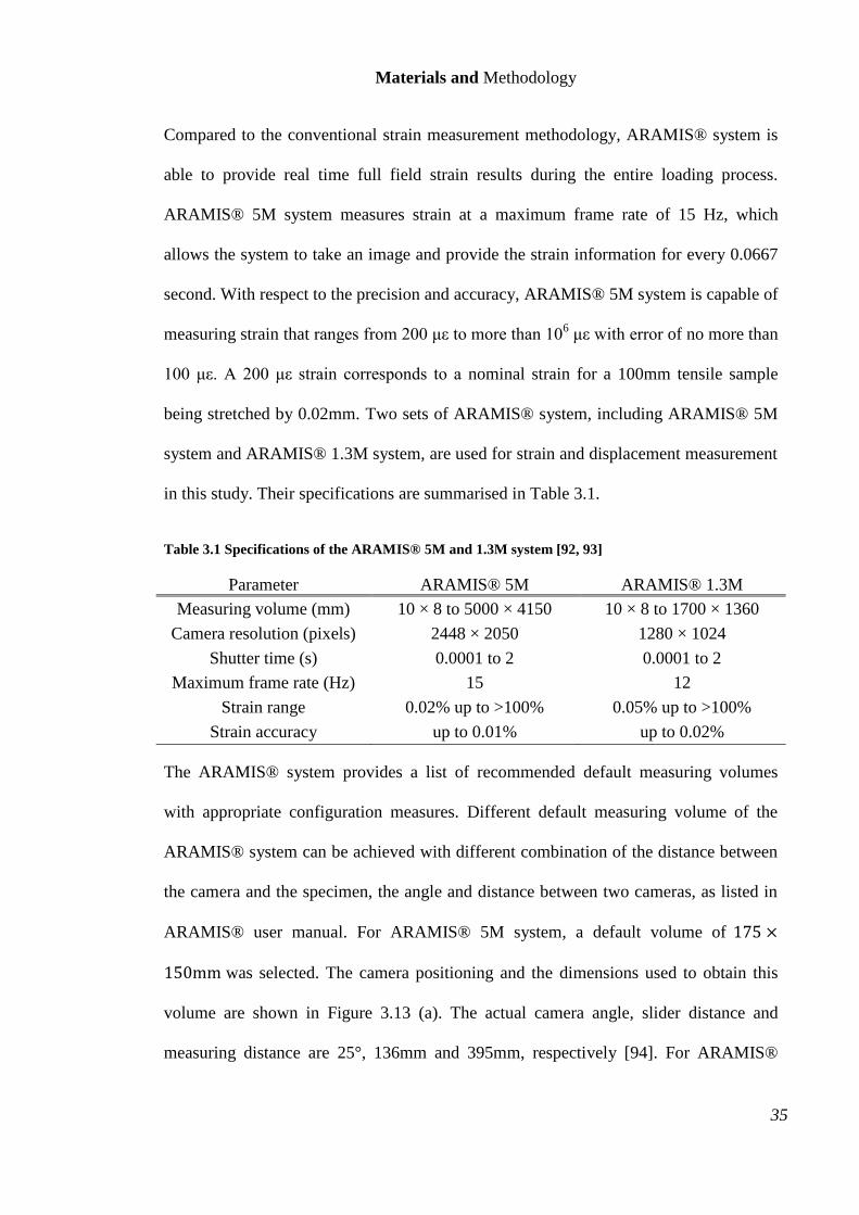
Materials and Methodology
35
Compared to the conventional strain measurement methodology, ARAMIS® system is
able to provide real time full field strain results during the entire loading process.
ARAMIS® 5M system measures strain at a maximum frame rate of 15 Hz, which
allows the system to take an image and provide the strain information for every 0.0667
second. With respect to the precision and accuracy, ARAMIS® 5M system is capable of
measuring strain that ranges from 200 με to more than 106 με with error of no more than
100 με. A 200 με strain corresponds to a nominal strain for a 100mm tensile sample
being stretched by 0.02mm. Two sets of ARAMIS® system, including ARAMIS® 5M
system and ARAMIS® 1.3M system, are used for strain and displacement measurement
in this study. Their specifications are summarised in Table 3.1.
Table 3.1 Specifications of the ARAMIS® 5M and 1.3M system [92, 93]
Parameter ARAMIS® 5M ARAMIS® 1.3M
Measuring volume (mm) 10 × 8 to 5000 × 4150 10 × 8 to 1700 × 1360
Camera resolution (pixels) 2448 × 2050 1280 × 1024
Shutter time (s) 0.0001 to 2 0.0001 to 2
Maximum frame rate (Hz) 15 12
Strain range 0.02% up to >100% 0.05% up to >100%
Strain accuracy up to 0.01% up to 0.02%
The ARAMIS® system provides a list of recommended default measuring volumes
with appropriate configuration measures. Different default measuring volume of the
ARAMIS® system can be achieved with different combination of the distance between
the camera and the specimen, the angle and distance between two cameras, as listed in
ARAMIS® user manual. For ARAMIS® 5M system, a default volume of 175 ×
150mm was selected. The camera positioning and the dimensions used to obtain this
volume are shown in Figure 3.13 (a). The actual camera angle, slider distance and
measuring distance are 25°, 136mm and 395mm, respectively [94]. For ARAMIS®
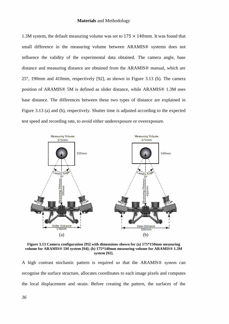
Materials and Methodology
36
1.3M system, the default measuring volume was set to 175 × 140mm. It was found that
small difference in the measuring volume between ARAMIS® systems does not
influence the validity of the experimental data obtained. The camera angle, base
distance and measuring distance are obtained from the ARAMIS® manual, which are
25°, 190mm and 410mm, respectively [92], as shown in Figure 3.13 (b). The camera
position of ARAMIS® 5M is defined as slider distance, while ARAMIS® 1.3M uses
base distance. The differences between these two types of distance are explained in
Figure 3.13 (a) and (b), respectively. Shutter time is adjusted according to the expected
test speed and recording rate, to avoid either underexposure or overexposure.
(a) (b)
Figure 3.13 Camera configuration [95] with dimensions shown for (a) 175*150mm measuring
volume for ARAMIS® 5M system [94]; (b) 175*140mm measuring volume for ARAMIS® 1.3M
system [92].
A high contrast stochastic pattern is required so that the ARAMIS® system can
recognise the surface structure, allocates coordinates to each image pixels and computes
the local displacement and strain. Before creating the pattern, the surfaces of the
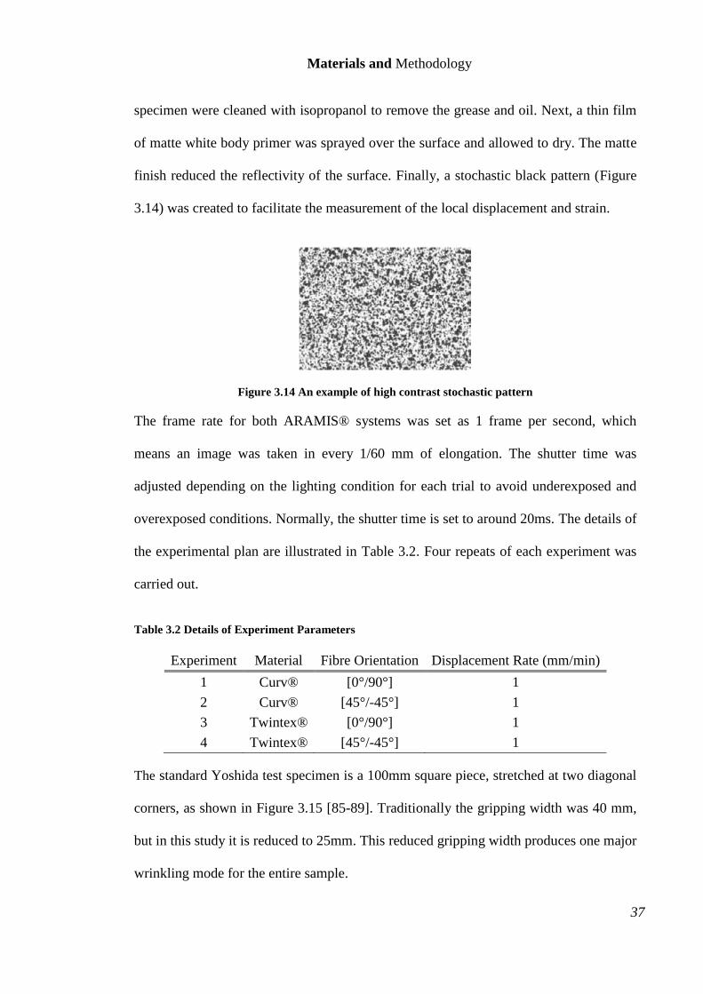
Materials and Methodology
37
specimen were cleaned with isopropanol to remove the grease and oil. Next, a thin film
of matte white body primer was sprayed over the surface and allowed to dry. The matte
finish reduced the reflectivity of the surface. Finally, a stochastic black pattern (Figure
3.14) was created to facilitate the measurement of the local displacement and strain.
Figure 3.14 An example of high contrast stochastic pattern
The frame rate for both ARAMIS® systems was set as 1 frame per second, which
means an image was taken in every 1/60 mm of elongation. The shutter time was
adjusted depending on the lighting condition for each trial to avoid underexposed and
overexposed conditions. Normally, the shutter time is set to around 20ms. The details of
the experimental plan are illustrated in Table 3.2. Four repeats of each experiment was
carried out.
Table 3.2 Details of Experiment Parameters
Experiment Material Fibre Orientation Displacement Rate (mm/min)
1 Curv® [0°/90°] 1
2 Curv® [45°/-45°] 1
3 Twintex® [0°/90°] 1
4 Twintex® [45°/-45°] 1
The standard Yoshida test specimen is a 100mm square piece, stretched at two diagonal
corners, as shown in Figure 3.15 [85-89]. Traditionally the gripping width was 40 mm,
but in this study it is reduced to 25mm. This reduced gripping width produces one major
wrinkling mode for the entire sample.
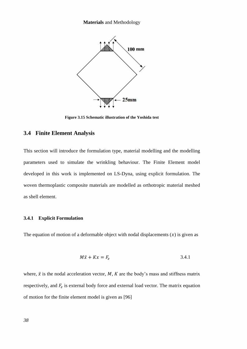
Materials and Methodology
38
Figure 3.15 Schematic illustration of the Yoshida test
3.4 Finite Element Analysis
This section will introduce the formulation type, material modelling and the modelling
parameters used to simulate the wrinkling behaviour. The Finite Element model
developed in this work is implemented on LS-Dyna, using explicit formulation. The
woven thermoplastic composite materials are modelled as orthotropic material meshed
as shell element.
3.4.1 Explicit Formulation
The equation of motion of a deformable object with nodal displacements (𝑥) is given as
𝑀�̈� + 𝐾𝑥 = 𝐹𝑒 3.4.1
where, �̈� is the nodal acceleration vector, 𝑀, 𝐾 are the body’s mass and stiffness matrix
respectively, and 𝐹𝑒 is external body force and external load vector. The matrix equation
of motion for the finite element model is given as [96]
Materials and Methodology
39
𝑅 = 𝑀�̈� + 𝐹𝑖 − 𝐹𝑒 3.4.2
where 𝐹𝑖 denotes internal force and R is residual force vector. In explicit method, the
displacement is a function of time, which means that the velocity and nodal acceleration
as well as the mass and damping are considered in this scheme. The equation below
expresses dynamic equilibrium condition at the instant of time [97, 98]
𝑀𝑡�̈�𝑡 + 𝐾𝑡𝑥𝑡 = 𝐹𝑒𝑡 3.4.3
where the term (𝐾𝑡𝑥𝑡) represents the internal forces generated from the stiffness. By
applying central difference integration rule, the velocities and displacements can be
solved as
�̇�𝑡+∆𝑡2 = (M𝑡)−1(𝐹𝑒
𝑡 − 𝐾𝑡𝑥𝑡)∆𝑡𝑡+∆𝑡2 + �̇�𝑡−
∆𝑡2 3.4.4
𝑢𝑡+∆𝑡 = 𝑢𝑡 + �̇�𝑡+∆𝑡2 ∆𝑡𝑡+∆𝑡 3.4.5
The equation of motion for the body is integrated with an explicit central difference
integration rule
�̇�𝑡+∆𝑡2 = �̇�𝑡−
∆𝑡2 +
(∆𝑡𝑡+∆𝑡 + ∆𝑡𝑡)
2�̈�𝑡 3.4.6
𝑢𝑡+∆𝑡 = 𝑢𝑡 + �̇�𝑡+∆𝑡2 ∆𝑡𝑡+∆𝑡 3.4.7
where �̇� is velocity, �̈� is the acceleration and 𝑡 −∆𝑡
2 and 𝑡 +
∆𝑡
2 indicate the increment
number and mid-increment number, respectively.
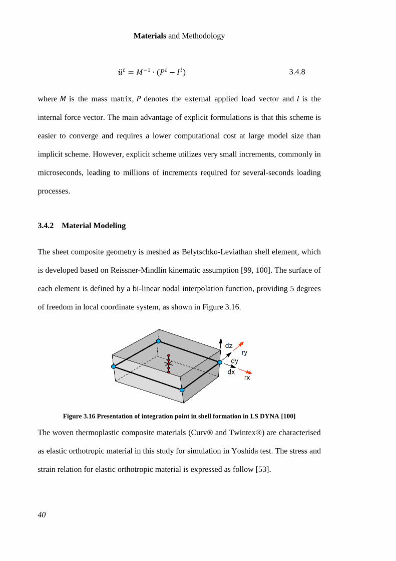
Materials and Methodology
40
�̈�𝑡 = 𝑀−1 ∙ (𝑃𝑖 − 𝐼𝑖) 3.4.8
where 𝑀 is the mass matrix, 𝑃 denotes the external applied load vector and 𝐼 is the
internal force vector. The main advantage of explicit formulations is that this scheme is
easier to converge and requires a lower computational cost at large model size than
implicit scheme. However, explicit scheme utilizes very small increments, commonly in
microseconds, leading to millions of increments required for several-seconds loading
processes.
3.4.2 Material Modeling
The sheet composite geometry is meshed as Belytschko-Leviathan shell element, which
is developed based on Reissner-Mindlin kinematic assumption [99, 100]. The surface of
each element is defined by a bi-linear nodal interpolation function, providing 5 degrees
of freedom in local coordinate system, as shown in Figure 3.16.
Figure 3.16 Presentation of integration point in shell formation in LS DYNA [100]
The woven thermoplastic composite materials (Curv® and Twintex®) are characterised
as elastic orthotropic material in this study for simulation in Yoshida test. The stress and
strain relation for elastic orthotropic material is expressed as follow [53].
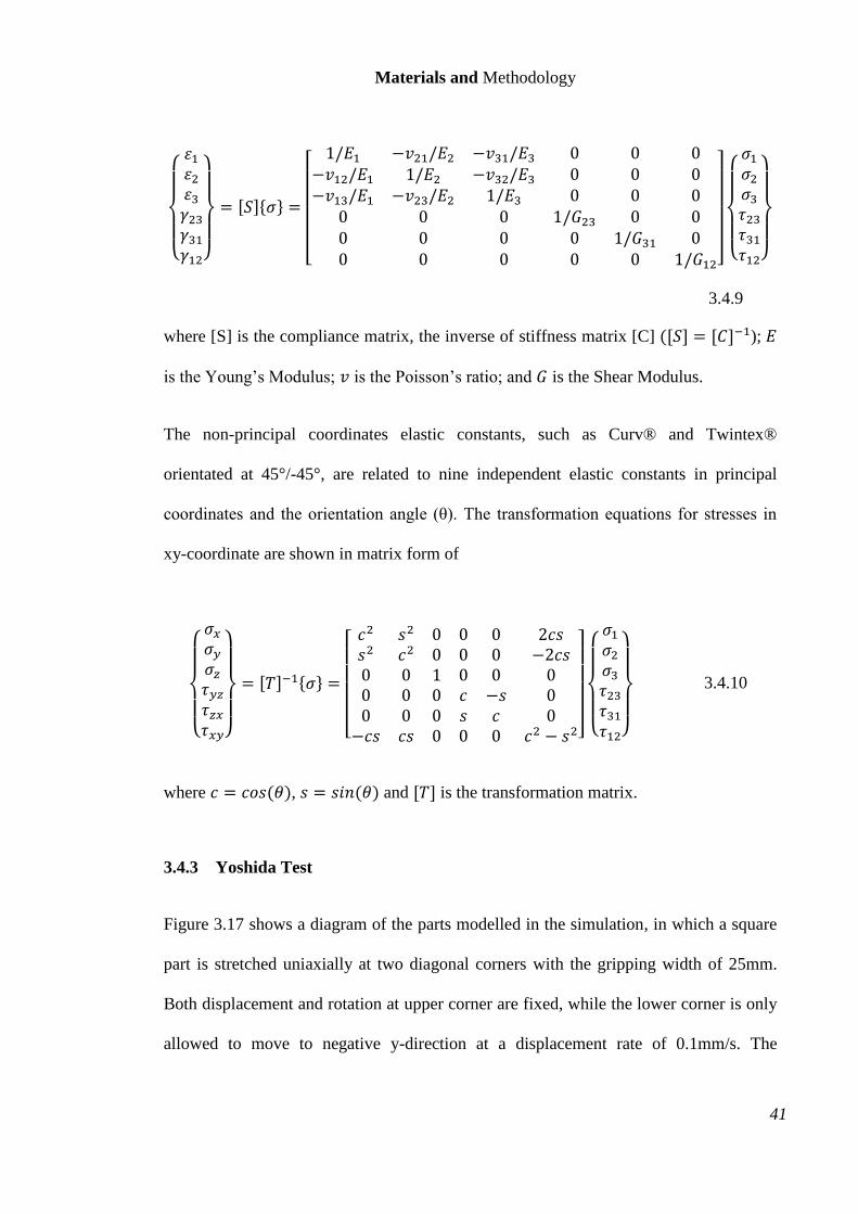
Materials and Methodology
41
{
𝜀1𝜀2𝜀3𝛾23𝛾31𝛾12}
= [𝑆]{𝜎} =
[ 1/𝐸1 −𝑣21/𝐸2 −𝑣31/𝐸3 0 0 0
−𝑣12/𝐸1 1/𝐸2 −𝑣32/𝐸3 0 0 0−𝑣13/𝐸1 −𝑣23/𝐸2 1/𝐸3 0 0 0
0 0 0 1/𝐺23 0 00 0 0 0 1/𝐺31 00 0 0 0 0 1/𝐺12]
{
𝜎1𝜎2𝜎3𝜏23𝜏31𝜏12}
3.4.9
where [S] is the compliance matrix, the inverse of stiffness matrix [C] ([𝑆] = [𝐶]−1); 𝐸
is the Young’s Modulus; 𝑣 is the Poisson’s ratio; and 𝐺 is the Shear Modulus.
The non-principal coordinates elastic constants, such as Curv® and Twintex®
orientated at 45°/-45°, are related to nine independent elastic constants in principal
coordinates and the orientation angle (θ). The transformation equations for stresses in
xy-coordinate are shown in matrix form of
{
𝜎𝑥𝜎𝑦𝜎𝑧𝜏𝑦𝑧𝜏𝑧𝑥𝜏𝑥𝑦}
= [𝑇]−1{𝜎} =
[ 𝑐2 𝑠2 0 0 0 2𝑐𝑠𝑠2 𝑐2 0 0 0 −2𝑐𝑠0 0 1 0 0 00 0 0 𝑐 −𝑠 00 0 0 𝑠 𝑐 0−𝑐𝑠 𝑐𝑠 0 0 0 𝑐2 − 𝑠2]
{
𝜎1𝜎2𝜎3𝜏23𝜏31𝜏12}
3.4.10
where 𝑐 = 𝑐𝑜𝑠(𝜃), 𝑠 = 𝑠𝑖𝑛(𝜃) and [𝑇] is the transformation matrix.
3.4.3 Yoshida Test
Figure 3.17 shows a diagram of the parts modelled in the simulation, in which a square
part is stretched uniaxially at two diagonal corners with the gripping width of 25mm.
Both displacement and rotation at upper corner are fixed, while the lower corner is only
allowed to move to negative y-direction at a displacement rate of 0.1mm/s. The
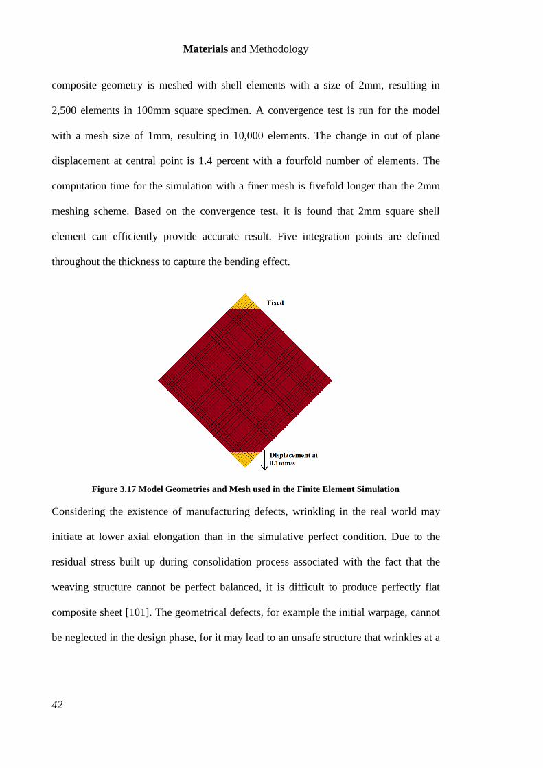
Materials and Methodology
42
composite geometry is meshed with shell elements with a size of 2mm, resulting in
2,500 elements in 100mm square specimen. A convergence test is run for the model
with a mesh size of 1mm, resulting in 10,000 elements. The change in out of plane
displacement at central point is 1.4 percent with a fourfold number of elements. The
computation time for the simulation with a finer mesh is fivefold longer than the 2mm
meshing scheme. Based on the convergence test, it is found that 2mm square shell
element can efficiently provide accurate result. Five integration points are defined
throughout the thickness to capture the bending effect.
Figure 3.17 Model Geometries and Mesh used in the Finite Element Simulation
Considering the existence of manufacturing defects, wrinkling in the real world may
initiate at lower axial elongation than in the simulative perfect condition. Due to the
residual stress built up during consolidation process associated with the fact that the
weaving structure cannot be perfect balanced, it is difficult to produce perfectly flat
composite sheet [101]. The geometrical defects, for example the initial warpage, cannot
be neglected in the design phase, for it may lead to an unsafe structure that wrinkles at a
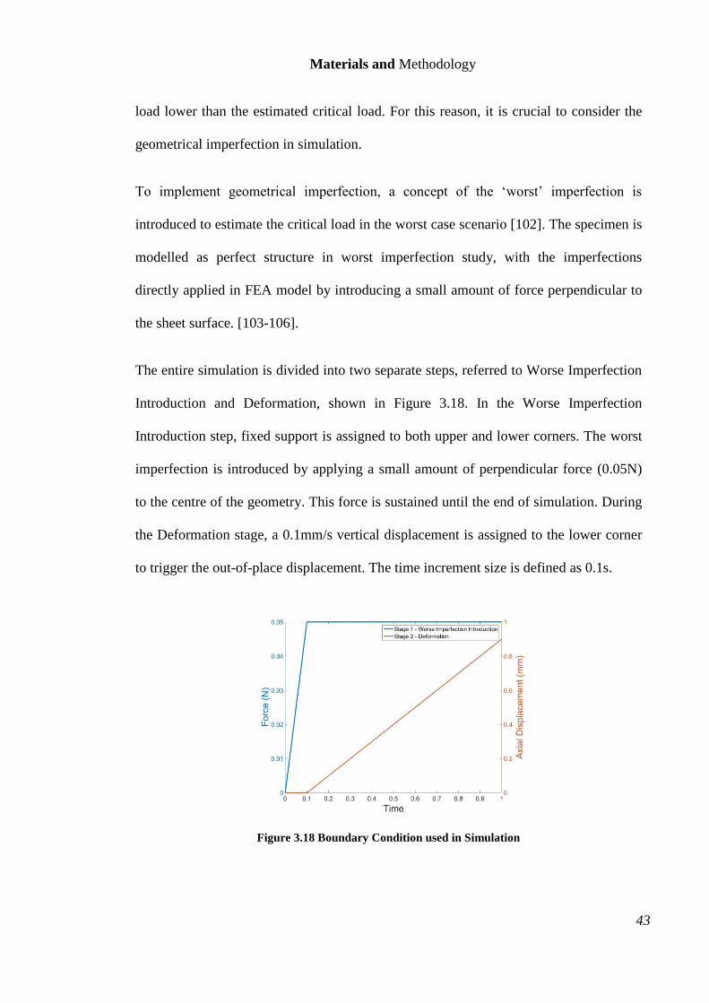
Materials and Methodology
43
load lower than the estimated critical load. For this reason, it is crucial to consider the
geometrical imperfection in simulation.
To implement geometrical imperfection, a concept of the ‘worst’ imperfection is
introduced to estimate the critical load in the worst case scenario [102]. The specimen is
modelled as perfect structure in worst imperfection study, with the imperfections
directly applied in FEA model by introducing a small amount of force perpendicular to
the sheet surface. [103-106].
The entire simulation is divided into two separate steps, referred to Worse Imperfection
Introduction and Deformation, shown in Figure 3.18. In the Worse Imperfection
Introduction step, fixed support is assigned to both upper and lower corners. The worst
imperfection is introduced by applying a small amount of perpendicular force (0.05N)
to the centre of the geometry. This force is sustained until the end of simulation. During
the Deformation stage, a 0.1mm/s vertical displacement is assigned to the lower corner
to trigger the out-of-place displacement. The time increment size is defined as 0.1s.
Figure 3.18 Boundary Condition used in Simulation
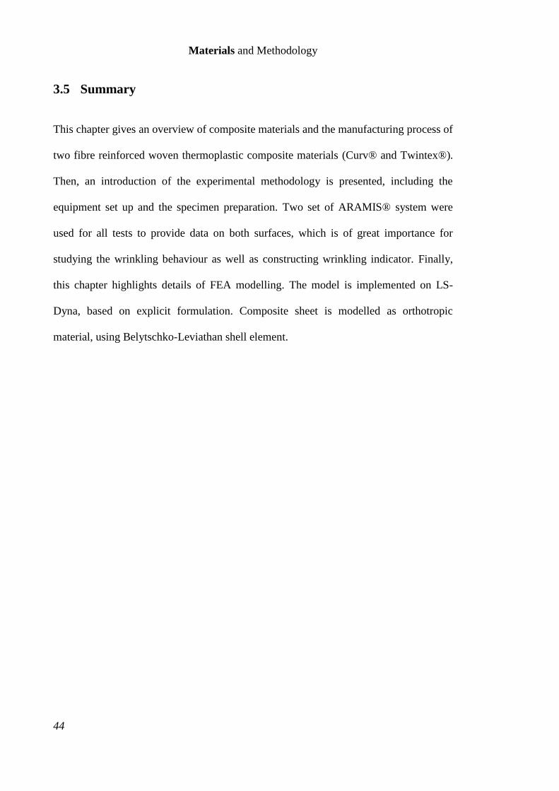
Materials and Methodology
44
3.5 Summary
This chapter gives an overview of composite materials and the manufacturing process of
two fibre reinforced woven thermoplastic composite materials (Curv® and Twintex®).
Then, an introduction of the experimental methodology is presented, including the
equipment set up and the specimen preparation. Two set of ARAMIS® system were
used for all tests to provide data on both surfaces, which is of great importance for
studying the wrinkling behaviour as well as constructing wrinkling indicator. Finally,
this chapter highlights details of FEA modelling. The model is implemented on LS-
Dyna, based on explicit formulation. Composite sheet is modelled as orthotropic
material, using Belytschko-Leviathan shell element.
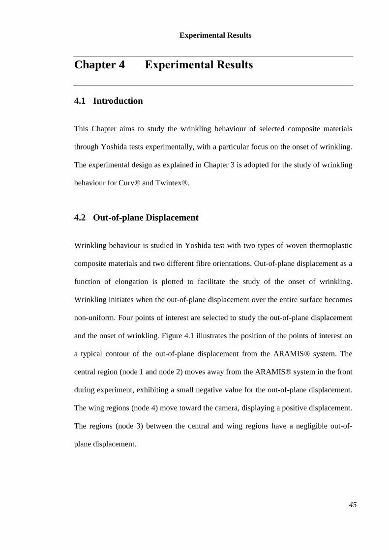
Experimental Results
45
Chapter 4 Experimental Results
4.1 Introduction
This Chapter aims to study the wrinkling behaviour of selected composite materials
through Yoshida tests experimentally, with a particular focus on the onset of wrinkling.
The experimental design as explained in Chapter 3 is adopted for the study of wrinkling
behaviour for Curv® and Twintex®.
4.2 Out-of-plane Displacement
Wrinkling behaviour is studied in Yoshida test with two types of woven thermoplastic
composite materials and two different fibre orientations. Out-of-plane displacement as a
function of elongation is plotted to facilitate the study of the onset of wrinkling.
Wrinkling initiates when the out-of-plane displacement over the entire surface becomes
non-uniform. Four points of interest are selected to study the out-of-plane displacement
and the onset of wrinkling. Figure 4.1 illustrates the position of the points of interest on
a typical contour of the out-of-plane displacement from the ARAMIS® system. The
central region (node 1 and node 2) moves away from the ARAMIS® system in the front
during experiment, exhibiting a small negative value for the out-of-plane displacement.
The wing regions (node 4) move toward the camera, displaying a positive displacement.
The regions (node 3) between the central and wing regions have a negligible out-of-
plane displacement.
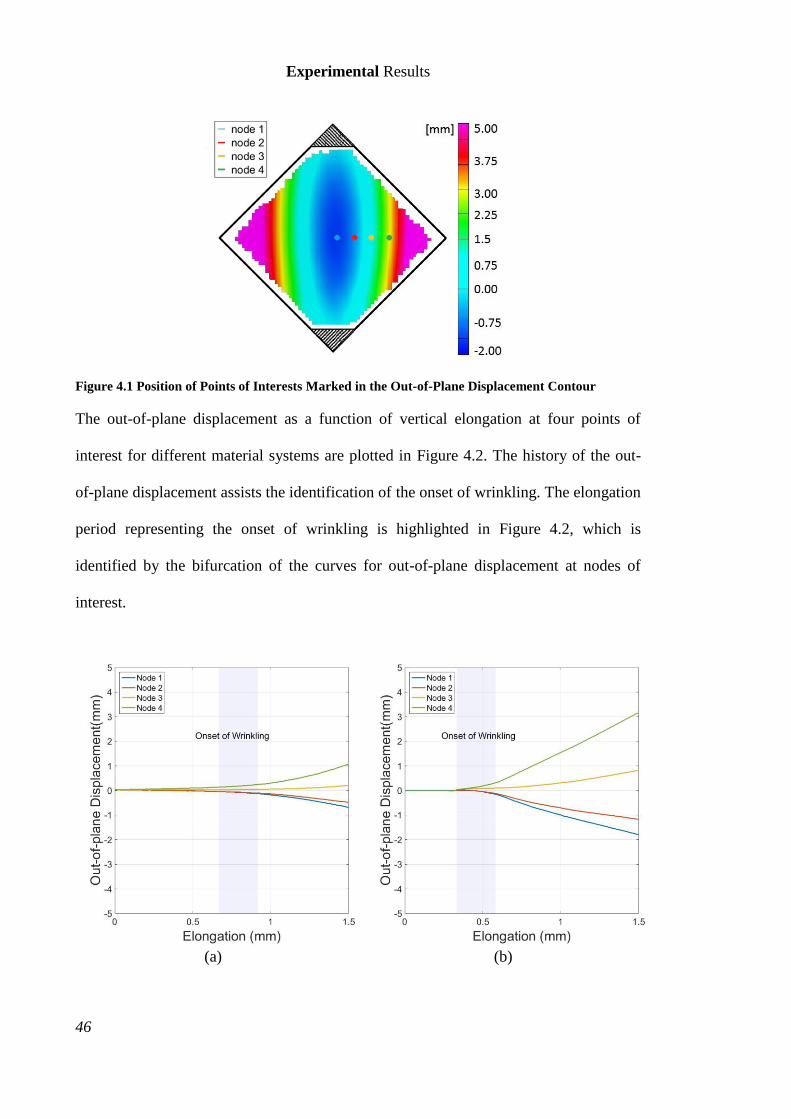
Experimental Results
46
Figure 4.1 Position of Points of Interests Marked in the Out-of-Plane Displacement Contour
The out-of-plane displacement as a function of vertical elongation at four points of
interest for different material systems are plotted in Figure 4.2. The history of the out-
of-plane displacement assists the identification of the onset of wrinkling. The elongation
period representing the onset of wrinkling is highlighted in Figure 4.2, which is
identified by the bifurcation of the curves for out-of-plane displacement at nodes of
interest.
(a) (b)
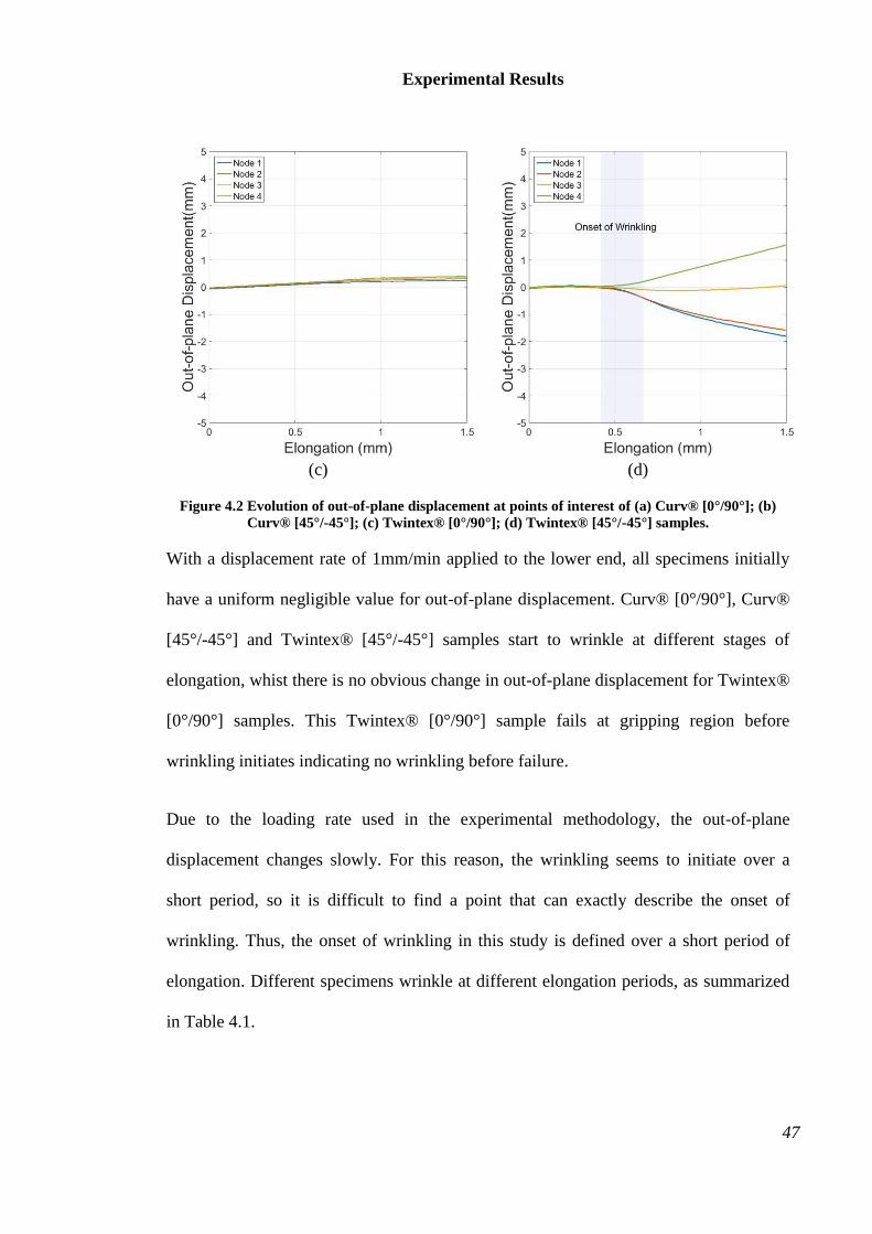
Experimental Results
47
(c) (d)
Figure 4.2 Evolution of out-of-plane displacement at points of interest of (a) Curv® [0°/90°]; (b)
Curv® [45°/-45°]; (c) Twintex® [0°/90°]; (d) Twintex® [45°/-45°] samples.
With a displacement rate of 1mm/min applied to the lower end, all specimens initially
have a uniform negligible value for out-of-plane displacement. Curv® [0°/90°], Curv®
[45°/-45°] and Twintex® [45°/-45°] samples start to wrinkle at different stages of
elongation, whist there is no obvious change in out-of-plane displacement for Twintex®
[0°/90°] samples. This Twintex® [0°/90°] sample fails at gripping region before
wrinkling initiates indicating no wrinkling before failure.
Due to the loading rate used in the experimental methodology, the out-of-plane
displacement changes slowly. For this reason, the wrinkling seems to initiate over a
short period, so it is difficult to find a point that can exactly describe the onset of
wrinkling. Thus, the onset of wrinkling in this study is defined over a short period of
elongation. Different specimens wrinkle at different elongation periods, as summarized
in Table 4.1.
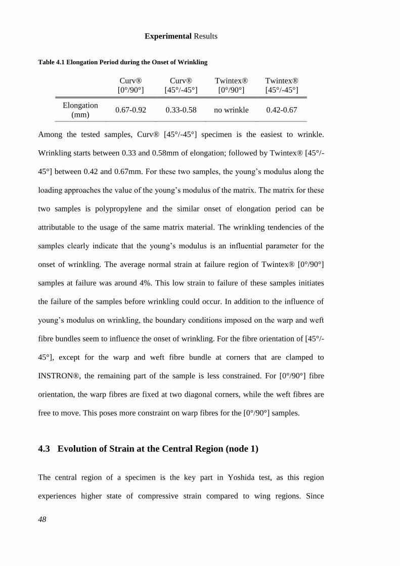
Experimental Results
48
Table 4.1 Elongation Period during the Onset of Wrinkling
Curv®
[0°/90°]
Curv®
[45°/-45°]
Twintex®
[0°/90°]
Twintex®
[45°/-45°]
Elongation
(mm) 0.67-0.92 0.33-0.58 no wrinkle 0.42-0.67
Among the tested samples, Curv® [45°/-45°] specimen is the easiest to wrinkle.
Wrinkling starts between 0.33 and 0.58mm of elongation; followed by Twintex® [45°/-
45°] between 0.42 and 0.67mm. For these two samples, the young’s modulus along the
loading approaches the value of the young’s modulus of the matrix. The matrix for these
two samples is polypropylene and the similar onset of elongation period can be
attributable to the usage of the same matrix material. The wrinkling tendencies of the
samples clearly indicate that the young’s modulus is an influential parameter for the
onset of wrinkling. The average normal strain at failure region of Twintex® [0°/90°]
samples at failure was around 4%. This low strain to failure of these samples initiates
the failure of the samples before wrinkling could occur. In addition to the influence of
young’s modulus on wrinkling, the boundary conditions imposed on the warp and weft
fibre bundles seem to influence the onset of wrinkling. For the fibre orientation of [45°/-
45°], except for the warp and weft fibre bundle at corners that are clamped to
INSTRON®, the remaining part of the sample is less constrained. For [0°/90°] fibre
orientation, the warp fibres are fixed at two diagonal corners, while the weft fibres are
free to move. This poses more constraint on warp fibres for the [0°/90°] samples.
4.3 Evolution of Strain at the Central Region (node 1)
The central region of a specimen is the key part in Yoshida test, as this region
experiences higher state of compressive strain compared to wing regions. Since
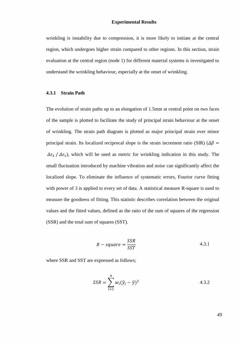
Experimental Results
49
wrinkling is instability due to compression, it is more likely to initiate at the central
region, which undergoes higher strain compared to other regions. In this section, strain
evaluation at the central region (node 1) for different material systems is investigated to
understand the wrinkling behaviour, especially at the onset of wrinkling.
4.3.1 Strain Path
The evolution of strain paths up to an elongation of 1.5mm at central point on two faces
of the sample is plotted to facilitate the study of principal strain behaviour at the onset
of wrinkling. The strain path diagram is plotted as major principal strain over minor
principal strain. Its localized reciprocal slope is the strain increment ratio (SIR) (𝛥𝛽 =
𝛥𝜀2 / 𝛥𝜀1), which will be used as metric for wrinkling indication in this study. The
small fluctuation introduced by machine vibration and noise can significantly affect the
localized slope. To eliminate the influence of systematic errors, Fourior curve fitting
with power of 3 is applied to every set of data. A statistical measure R-square is used to
measure the goodness of fitting. This statistic describes correlation between the original
values and the fitted values, defined as the ratio of the sum of squares of the regression
(SSR) and the total sum of squares (SST).
𝑅 − 𝑠𝑞𝑢𝑎𝑟𝑒 =𝑆𝑆𝑅
𝑆𝑆𝑇 4.3.1
where SSR and SST are expressed as follows;
𝑆𝑆𝑅 =∑𝑤𝑖(�̂�𝑖 − �̅�)2
𝑛
𝑖=1
4.3.2
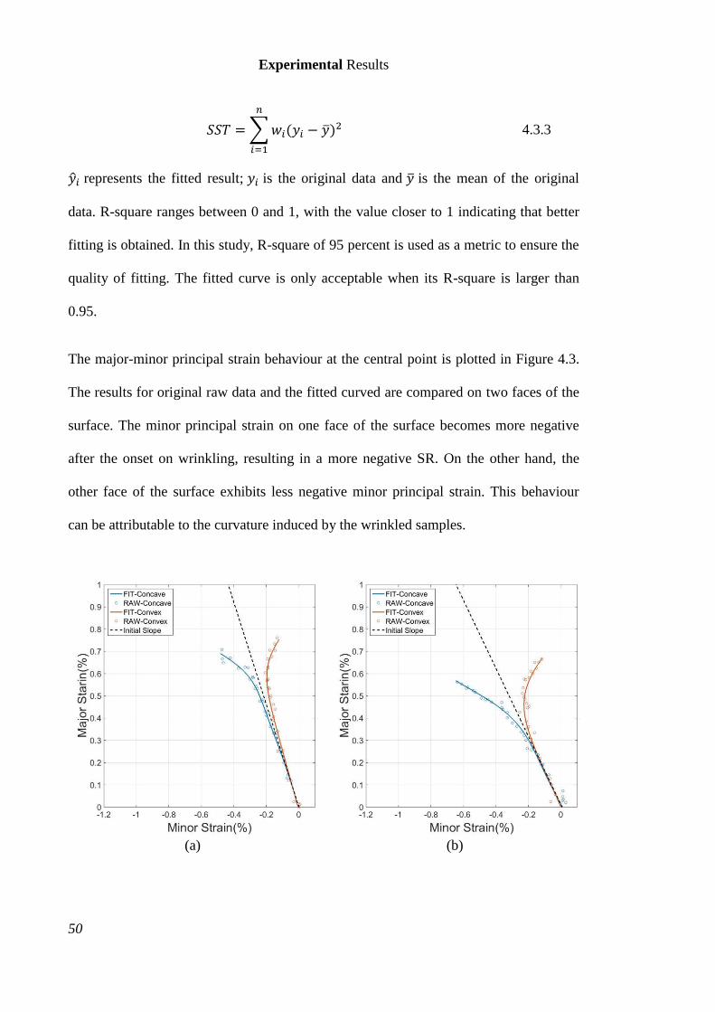
Experimental Results
50
𝑆𝑆𝑇 =∑𝑤𝑖(𝑦𝑖 − �̅�)2
𝑛
𝑖=1
4.3.3
�̂�𝑖 represents the fitted result; 𝑦𝑖 is the original data and �̅� is the mean of the original
data. R-square ranges between 0 and 1, with the value closer to 1 indicating that better
fitting is obtained. In this study, R-square of 95 percent is used as a metric to ensure the
quality of fitting. The fitted curve is only acceptable when its R-square is larger than
0.95.
The major-minor principal strain behaviour at the central point is plotted in Figure 4.3.
The results for original raw data and the fitted curved are compared on two faces of the
surface. The minor principal strain on one face of the surface becomes more negative
after the onset on wrinkling, resulting in a more negative SR. On the other hand, the
other face of the surface exhibits less negative minor principal strain. This behaviour
can be attributable to the curvature induced by the wrinkled samples.
(a) (b)
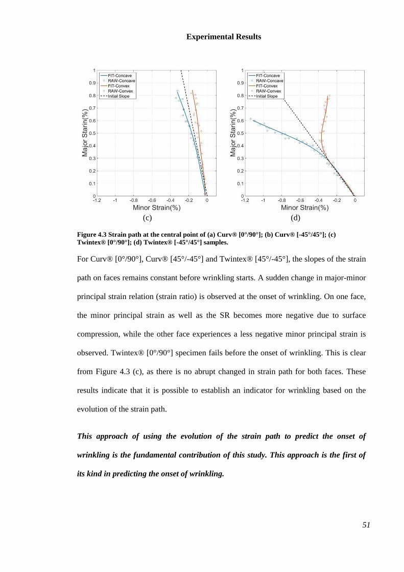
Experimental Results
51
(c) (d)
Figure 4.3 Strain path at the central point of (a) Curv® [0°/90°]; (b) Curv® [-45°/45°]; (c)
Twintex® [0°/90°]; (d) Twintex® [-45°/45°] samples.
For Curv® [0°/90°], Curv® [45°/-45°] and Twintex® [45°/-45°], the slopes of the strain
path on faces remains constant before wrinkling starts. A sudden change in major-minor
principal strain relation (strain ratio) is observed at the onset of wrinkling. On one face,
the minor principal strain as well as the SR becomes more negative due to surface
compression, while the other face experiences a less negative minor principal strain is
observed. Twintex® [0°/90°] specimen fails before the onset of wrinkling. This is clear
from Figure 4.3 (c), as there is no abrupt changed in strain path for both faces. These
results indicate that it is possible to establish an indicator for wrinkling based on the
evolution of the strain path.
This approach of using the evolution of the strain path to predict the onset of
wrinkling is the fundamental contribution of this study. This approach is the first of
its kind in predicting the onset of wrinkling.
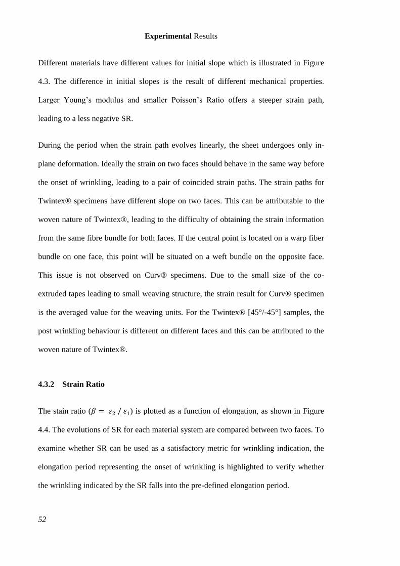
Experimental Results
52
Different materials have different values for initial slope which is illustrated in Figure
4.3. The difference in initial slopes is the result of different mechanical properties.
Larger Young’s modulus and smaller Poisson’s Ratio offers a steeper strain path,
leading to a less negative SR.
During the period when the strain path evolves linearly, the sheet undergoes only in-
plane deformation. Ideally the strain on two faces should behave in the same way before
the onset of wrinkling, leading to a pair of coincided strain paths. The strain paths for
Twintex® specimens have different slope on two faces. This can be attributable to the
woven nature of Twintex®, leading to the difficulty of obtaining the strain information
from the same fibre bundle for both faces. If the central point is located on a warp fiber
bundle on one face, this point will be situated on a weft bundle on the opposite face.
This issue is not observed on Curv® specimens. Due to the small size of the co-
extruded tapes leading to small weaving structure, the strain result for Curv® specimen
is the averaged value for the weaving units. For the Twintex® [45°/-45°] samples, the
post wrinkling behaviour is different on different faces and this can be attributed to the
woven nature of Twintex®.
4.3.2 Strain Ratio
The stain ratio (𝛽 = 𝜀2 / 𝜀1) is plotted as a function of elongation, as shown in Figure
4.4. The evolutions of SR for each material system are compared between two faces. To
examine whether SR can be used as a satisfactory metric for wrinkling indication, the
elongation period representing the onset of wrinkling is highlighted to verify whether
the wrinkling indicated by the SR falls into the pre-defined elongation period.
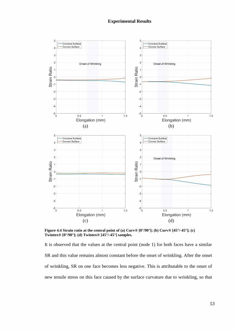
Experimental Results
53
(a) (b)
(c) (d)
Figure 4.4 Strain ratio at the central point of (a) Curv® [0°/90°]; (b) Curv® [45°/-45°]; (c)
Twintex® [0°/90°]; (d) Twintex® [45°/-45°] samples.
It is observed that the values at the central point (node 1) for both faces have a similar
SR and this value remains almost constant before the onset of wrinkling. After the onset
of wrinkling, SR on one face becomes less negative. This is attributable to the onset of
new tensile stress on this face caused by the surface curvature due to wrinkling, so that
Experimental Results
54
the compressive stress is reduced. On the opposite face, a more negative SR is obtained,
since the surface curvature adds more compression to the central part of this face.
For the wrinkled samples, SR moves away from its initial value at different elongations,
indicating the onset of wrinkling. These abrupt changes in SR are in good agreement to
the elongation period obtained from the out-of-plane displacement. Curv® [45°/-45°]
samples exhibit abrupt changes at the lowest deformation; followed by Twintex® [45°/-
45°] and Curv® [0°/90°] samples. The figure for Twintex® [0°/90°] samples shows no
obvious variation, because no wrinkling is observed.
However, in some samples, like Curv® [0°/90°] specimens, the changes are not abrupt,
which may lead to a difficulty in the abrupt change quantification and identification. For
this reason, establishing a wrinkling indicator based on the abrupt change in SR may fail
to detect wrinkling.
4.3.3 Strain Increment Ratio
Strain increment ratio 𝛥𝛽 = 𝛥𝜀2 / 𝛥𝜀1 is introduced to indicate the initiation of
wrinkling. Here, 𝛥𝜀2 is the change in minor principal strain for one time increment and
𝛥𝜀1 is the change in major principal strain for the same period of time. The SIR is
plotted as a function of elongation, as shown in Figure 4.5.
Experimental Results
55
(a) (b)
(c) (d)
Figure 4.5 Strain increment ratio at the central point of (a) Curv® [0°/90°]; (b) Curv® [45°/-45°]; (c)
Twintex® [0°/90°]; (d) Twintex® [45°/-45°] samples.
Before the onset of wrinkling, the SIR at the central node is unchanged and two faces
exhibit a similar SIR. For Twintex® [0°/90°] samples, SIR appears to be constant over
the loading process, elucidating no wrinkling occurs, because it fails before the onset of
wrinkling. The initial SIR for Curv® [0°/90°], Curv® [45°/-45°] and Twintex® [45°/-
45°] samples are -0.45, -0.6 and -0.95, respectively. The abrupt change in SIR is
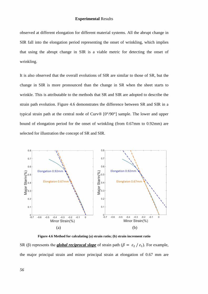
Experimental Results
56
observed at different elongation for different material systems. All the abrupt change in
SIR fall into the elongation period representing the onset of wrinkling, which implies
that using the abrupt change in SIR is a viable metric for detecting the onset of
wrinkling.
It is also observed that the overall evolutions of SIR are similar to those of SR, but the
change in SIR is more pronounced than the change in SR when the sheet starts to
wrinkle. This is attributable to the methods that SR and SIR are adopted to describe the
strain path evolution. Figure 4.6 demonstrates the difference between SR and SIR in a
typical strain path at the central node of Curv® [0°/90°] sample. The lower and upper
bound of elongation period for the onset of wrinkling (from 0.67mm to 0.92mm) are
selected for illustration the concept of SR and SIR.
(a) (b)
Figure 4.6 Method for calculating (a) strain ratio; (b) strain increment ratio
SR (β) represents the global reciprocal slope of strain path (𝛽 = 𝜀2 / 𝜀1). For example,
the major principal strain and minor principal strain at elongation of 0.67 mm are
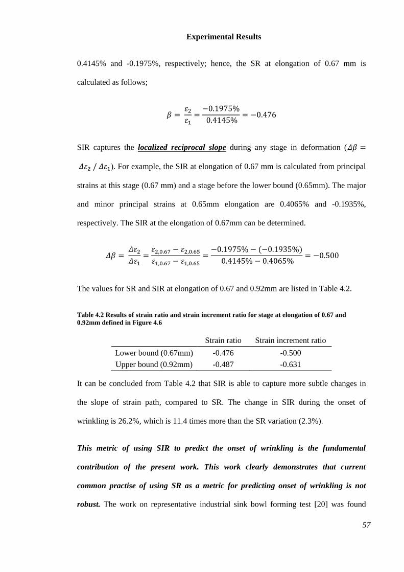
Experimental Results
57
0.4145% and -0.1975%, respectively; hence, the SR at elongation of 0.67 mm is
calculated as follows;
𝛽 = 𝜀2𝜀1=−0.1975%
0.4145%= −0.476
SIR captures the localized reciprocal slope during any stage in deformation (𝛥𝛽 =
𝛥𝜀2 / 𝛥𝜀1). For example, the SIR at elongation of 0.67 mm is calculated from principal
strains at this stage (0.67 mm) and a stage before the lower bound (0.65mm). The major
and minor principal strains at 0.65mm elongation are 0.4065% and -0.1935%,
respectively. The SIR at the elongation of 0.67mm can be determined.
𝛥𝛽 = 𝛥𝜀2𝛥𝜀1
=𝜀2,0.67 − 𝜀2,0.65𝜀1,0.67 − 𝜀1,0.65
=−0.1975% − (−0.1935%)
0.4145% − 0.4065%= −0.500
The values for SR and SIR at elongation of 0.67 and 0.92mm are listed in Table 4.2.
Table 4.2 Results of strain ratio and strain increment ratio for stage at elongation of 0.67 and
0.92mm defined in Figure 4.6
Strain ratio Strain increment ratio
Lower bound (0.67mm) -0.476 -0.500
Upper bound (0.92mm) -0.487 -0.631
It can be concluded from Table 4.2 that SIR is able to capture more subtle changes in
the slope of strain path, compared to SR. The change in SIR during the onset of
wrinkling is 26.2%, which is 11.4 times more than the SR variation (2.3%).
This metric of using SIR to predict the onset of wrinkling is the fundamental
contribution of the present work. This work clearly demonstrates that current
common practise of using SR as a metric for predicting onset of wrinkling is not
robust. The work on representative industrial sink bowl forming test [20] was found
Experimental Results
58
that wrinkling at the flange, corners of the walls and mid-part of the walls initiated at
different values of SR of approximately -1.0, -0.5 and 0.5, respectively. This
observation clearly demonstrates that using SR as a metric to predict wrinkling
behaviour is inadequate. It has been demonstrated in this work that the abrupt change in
strain path provides a robust metric predicting the onset of wrinkling.
4.4 Evolution of Strain Increment Ratio at Four Points of Interest
The feasibility of using SIR as a metric to indicate the onset of wrinkling is tested at
four nodes of interest on both faces. In this study, the comparison between two faces
will be carried out to study the overall evolution of SIR, but the correlation of the nodes
of interest between two faces will not be presented. Due to the woven nature of
composite material, a point on the warp fibre bundle on one face may appear on the
weft fibre bundle on the opposite face of the sample (especially on Twintex® samples).
Under the Yoshida test, fibre bundle at different orientation exhibiting different strain
behaviours, so that it is not fully meaningful to carry out a comparison between nodes
of interest on different faces. In addition to the woven nature, the size and the
arrangement of the facet cannot be adjusted to be exactly the same for two sets of
ARAMIS® systems, so it is not possible to generate the result from exactly the same
location but on different faces.
In this section, the comparison between the evolutions of SIR at four points of interest
on two faces will be carried out. This helps to explore the similarities and differences of
the overall strain evolution at the onset of wrinkling on two faces of the samples.
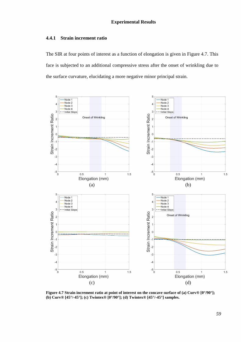
Experimental Results
59
4.4.1 Strain increment ratio
The SIR at four points of interest as a function of elongation is given in Figure 4.7. This
face is subjected to an additional compressive stress after the onset of wrinkling due to
the surface curvature, elucidating a more negative minor principal strain.
(a) (b)
(c) (d)
Figure 4.7 Strain increment ratio at point of interest on the concave surface of (a) Curv® [0°/90°];
(b) Curv® [45°/-45°]; (c) Twintex® [0°/90°]; (d) Twintex® [45°/-45°] samples.
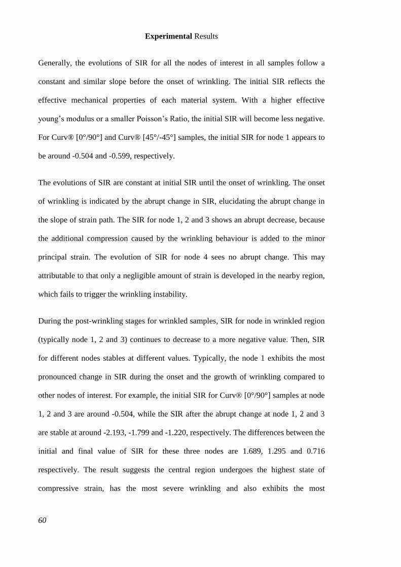
Experimental Results
60
Generally, the evolutions of SIR for all the nodes of interest in all samples follow a
constant and similar slope before the onset of wrinkling. The initial SIR reflects the
effective mechanical properties of each material system. With a higher effective
young’s modulus or a smaller Poisson’s Ratio, the initial SIR will become less negative.
For Curv® [0°/90°] and Curv® [45°/-45°] samples, the initial SIR for node 1 appears to
be around -0.504 and -0.599, respectively.
The evolutions of SIR are constant at initial SIR until the onset of wrinkling. The onset
of wrinkling is indicated by the abrupt change in SIR, elucidating the abrupt change in
the slope of strain path. The SIR for node 1, 2 and 3 shows an abrupt decrease, because
the additional compression caused by the wrinkling behaviour is added to the minor
principal strain. The evolution of SIR for node 4 sees no abrupt change. This may
attributable to that only a negligible amount of strain is developed in the nearby region,
which fails to trigger the wrinkling instability.
During the post-wrinkling stages for wrinkled samples, SIR for node in wrinkled region
(typically node 1, 2 and 3) continues to decrease to a more negative value. Then, SIR
for different nodes stables at different values. Typically, the node 1 exhibits the most
pronounced change in SIR during the onset and the growth of wrinkling compared to
other nodes of interest. For example, the initial SIR for Curv® [0°/90°] samples at node
1, 2 and 3 are around -0.504, while the SIR after the abrupt change at node 1, 2 and 3
are stable at around -2.193, -1.799 and -1.220, respectively. The differences between the
initial and final value of SIR for these three nodes are 1.689, 1.295 and 0.716
respectively. The result suggests the central region undergoes the highest state of
compressive strain, has the most severe wrinkling and also exhibits the most
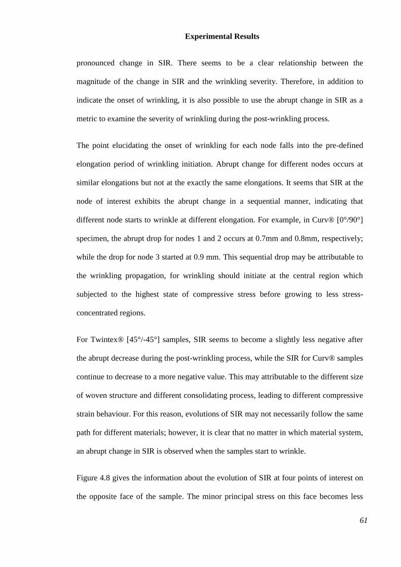
Experimental Results
61
pronounced change in SIR. There seems to be a clear relationship between the
magnitude of the change in SIR and the wrinkling severity. Therefore, in addition to
indicate the onset of wrinkling, it is also possible to use the abrupt change in SIR as a
metric to examine the severity of wrinkling during the post-wrinkling process.
The point elucidating the onset of wrinkling for each node falls into the pre-defined
elongation period of wrinkling initiation. Abrupt change for different nodes occurs at
similar elongations but not at the exactly the same elongations. It seems that SIR at the
node of interest exhibits the abrupt change in a sequential manner, indicating that
different node starts to wrinkle at different elongation. For example, in Curv® [0°/90°]
specimen, the abrupt drop for nodes 1 and 2 occurs at 0.7mm and 0.8mm, respectively;
while the drop for node 3 started at 0.9 mm. This sequential drop may be attributable to
the wrinkling propagation, for wrinkling should initiate at the central region which
subjected to the highest state of compressive stress before growing to less stress-
concentrated regions.
For Twintex® [45°/-45°] samples, SIR seems to become a slightly less negative after
the abrupt decrease during the post-wrinkling process, while the SIR for Curv® samples
continue to decrease to a more negative value. This may attributable to the different size
of woven structure and different consolidating process, leading to different compressive
strain behaviour. For this reason, evolutions of SIR may not necessarily follow the same
path for different materials; however, it is clear that no matter in which material system,
an abrupt change in SIR is observed when the samples start to wrinkle.
Figure 4.8 gives the information about the evolution of SIR at four points of interest on
the opposite face of the sample. The minor principal stress on this face becomes less
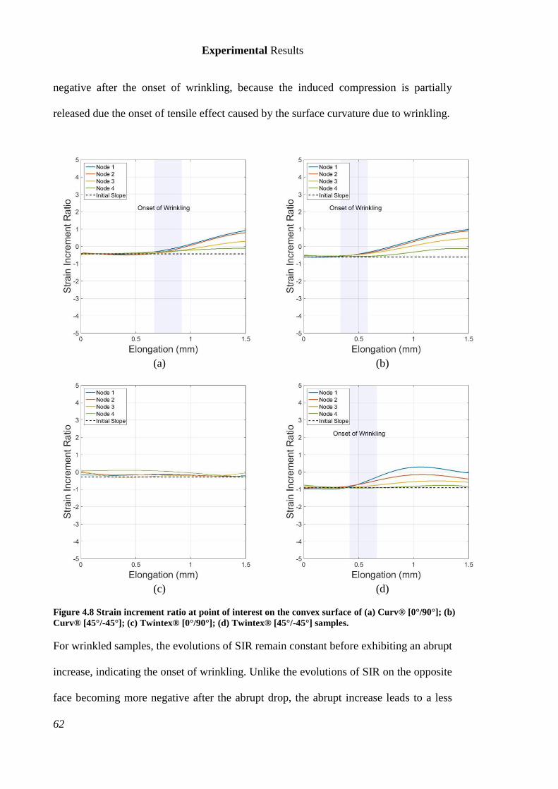
Experimental Results
62
negative after the onset of wrinkling, because the induced compression is partially
released due the onset of tensile effect caused by the surface curvature due to wrinkling.
(a) (b)
(c) (d)
Figure 4.8 Strain increment ratio at point of interest on the convex surface of (a) Curv® [0°/90°]; (b)
Curv® [45°/-45°]; (c) Twintex® [0°/90°]; (d) Twintex® [45°/-45°] samples.
For wrinkled samples, the evolutions of SIR remain constant before exhibiting an abrupt
increase, indicating the onset of wrinkling. Unlike the evolutions of SIR on the opposite
face becoming more negative after the abrupt drop, the abrupt increase leads to a less
Experimental Results
63
negative or even a positive SIR at large elongation. Due to the surface curvature
introduced by wrinkling behaviour, the induced compression on this face of the sample
is partially released, exhibiting a less negative minor principal strain and an abrupt rise
in SIR. These results clearly illustrated that using the abrupt change in SIR for
wrinkling indication can indicate the onset and the propagation of wrinkling on either
face of the sample.
For the unwrinkled Twintex® [0°/90°] sample, the evolution of SIR does not exhibit
any pronounced change, indicating no wrinkling starts before failure initiates. Owing to
that it seems that using the abrupt change in SIR as a metric is capable of indicating
wrinkling.
4.5 Summary
This chapter has studied the wrinkling behaviour on woven thermoplastic composite
materials through Yoshida tests experimentally, with a particular focus on the onset of
wrinkling. The elongation period for the onset of wrinkling is defined through analysing
the out-of-plane displacement. It is found that the abrupt change in principal strain path
can indicate the onset of wrinkling. SR and SIR are used as the metric to measure the
abrupt change in strain path. Compared to SR, developing a wrinkling indicator based
on SIR can capture more subtle change in strain path, offering an elevated robustness of
the indication of the onset of wrinkling. This metric of using the abrupt change in SIR to
predict the onset of wrinkling is the fundamental contribution of the present work.

Experimental Results
64
Development and Validation of Wrinkling Indicator
65
Chapter 5 Development and Validation of
Wrinkling Indicator
5.1 Introduction
This chapter aims to develop an indicator based on the SIR and then test the usefulness
of the proposed wrinkling indicator on the prediction of the onset of wrinkling in
Yoshida tests. This indicator is programmed in MATLAB script, using the information
extracted from FEA for predicting wrinkling. The modelling parameters as explained in
Chapter 3 are adopted for simulating the wrinkling behaviour in Yoshida test. The
predicted results are validated with the contour of out-of-plane displacement from
experiments. The prime motivation of developing a wrinkling indicator is to detect and
remove wrinkling for general forming practises, so that the validity of this indicator is
also explored in a series of dome forming tests.
5.2 The Development of Wrinkling Indicator for the Implementation
in Simulations
According to the experimental observations, the onset of wrinkling on either face of the
samples can be identified by the abrupt change in the slope of the strain path. The
metric of using SR or SIR has been tested and compared. It was concluded that
compared to the SR based indicator, using the abrupt change in SIR as a metric provides
a better indication of the abrupt change in slope of strain path. In this section, a
wrinkling indicator based on SIR will be developed for the implementation in
simulations.
Development and Validation of Wrinkling Indicator
66
SIR of every element at each time step is calculated from major and minor principal
strain at this time step and one step before. For example, the value for time step N is
calculated as follow,
∆𝛽𝑁 =∆𝜀2∆𝜀1
=𝜀2,𝑁 − 𝜀2,𝑁−1𝜀1,𝑁 − 𝜀1,𝑁−1
5.2.1
where ε1 and ε2 are the major principal strain and minor principal strain, respectively.
The time step ‘N’ ranges from the second to the last time step, because each SIR is
calculated from two sequential time steps.
To capture the abrupt change in SIR at the onset of wrinkling, critical SIR (∆𝛽𝑐𝑟) is
calculated element-wise and face-wise. If SIR at specific time exceeds the critical value,
the wrinkling indicator will turn on. The critical SIR is developed from the initial SIR
(∆𝛽𝑖𝑛𝑖𝑡𝑖𝑎𝑙) for each element. A factor of 1.1 is applied to initial SIR to quantify the
allowable abrupt change, so wrinkling is suggested to initiate when the change in SIR is
by either 10% larger or smaller than the initial SIR. The lower critical SIR (∆𝛽𝑐𝑟,𝑙𝑜𝑤𝑒𝑟)
is calculated from equation 5.2.2, while the equation 5.2.3 gives the upper critical SIR
(∆𝛽𝑐𝑟,upper). The lower critical SIR is more negative than the upper critical SIR.
∆𝛽𝑐𝑟,𝑙𝑜𝑤𝑒𝑟 = ∆𝛽𝑖𝑛𝑖𝑡𝑖𝑎𝑙 × 1.1 5.2.2
∆𝛽𝑐𝑟,upper = ∆𝛽𝑖𝑛𝑖𝑡𝑖𝑎𝑙/ 1.1 5.2.3
Initially, the evolution of SIR is in between of the lower and upper critical SIR,
indicating that the sample does not experience wrinkling. Once the SIR drops below the
lower critical SIR or rises over the upper critical SIR, the indicator at the corresponding

Development and Validation of Wrinkling Indicator
67
element at the specific stage will turn on. The relation 5.2.4 - 5.2.6 explain the method
of using the critical SIR for wrinkling indication.
∆𝛽𝑁 > ∆𝛽𝑐𝑟,𝑙𝑜𝑤𝑒𝑟
or
∆𝛽𝑐𝑟,𝑢𝑝𝑝𝑒𝑟 > ∆𝛽𝑁
Safe 5.2.4
∆𝛽𝑁 = ∆𝛽𝑐𝑟,𝑙𝑜𝑤𝑒𝑟
or
∆𝛽𝑐𝑟,𝑢𝑝𝑝𝑒𝑟 = ∆𝛽𝑁
Onset of Wrinkling 5.2.5
∆𝛽𝑁 < ∆𝛽𝑐𝑟,𝑙𝑜𝑤𝑒𝑟
or
∆𝛽𝑐𝑟,𝑢𝑝𝑝𝑒𝑟 < ∆𝛽𝑁
Wrinkle 5.2.6
An example of the centre point for Curv® [0°/90°] samples is presented to illustrate the
method adopted in the wrinkling indicator. The initial SIR for the face (namely face 1)
imposed to additional compression after wrinkling is -0.5039. The initial SIR for the
opposite face is -0.3725. Multiplying the factor of 1.1 to the initial SIR, the lower
critical SIR on two faces is -0.5543 and -0.4098, respectively. Dividing the initial SIR
by this factor, the upper critical SIR is given as -0.4581 and -0.3386, respectively.
Figure 5.1 presents the evolution of SIR up to 1mm and the critical SIR at the centre
point on two faces for Curv® [0°/90°] samples.
(a) (b)
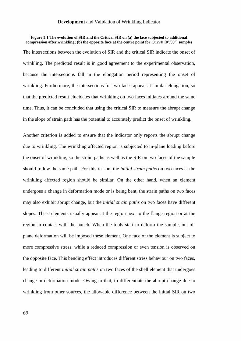
Development and Validation of Wrinkling Indicator
68
Figure 5.1 The evolution of SIR and the Critical SIR on (a) the face subjected to additional
compression after wrinkling; (b) the opposite face at the centre point for Curv® [0°/90°] samples
The intersections between the evolution of SIR and the critical SIR indicate the onset of
wrinkling. The predicted result is in good agreement to the experimental observation,
because the intersections fall in the elongation period representing the onset of
wrinkling. Furthermore, the intersections for two faces appear at similar elongation, so
that the predicted result elucidates that wrinkling on two faces initiates around the same
time. Thus, it can be concluded that using the critical SIR to measure the abrupt change
in the slope of strain path has the potential to accurately predict the onset of wrinkling.
Another criterion is added to ensure that the indicator only reports the abrupt change
due to wrinkling. The wrinkling affected region is subjected to in-plane loading before
the onset of wrinkling, so the strain paths as well as the SIR on two faces of the sample
should follow the same path. For this reason, the initial strain paths on two faces at the
wrinkling affected region should be similar. On the other hand, when an element
undergoes a change in deformation mode or is being bent, the strain paths on two faces
may also exhibit abrupt change, but the initial strain paths on two faces have different
slopes. These elements usually appear at the region next to the flange region or at the
region in contact with the punch. When the tools start to deform the sample, out-of-
plane deformation will be imposed these element. One face of the element is subject to
more compressive stress, while a reduced compression or even tension is observed on
the opposite face. This bending effect introduces different stress behaviour on two faces,
leading to different initial strain paths on two faces of the shell element that undergoes
change in deformation mode. Owing to that, to differentiate the abrupt change due to
wrinkling from other sources, the allowable difference between the initial SIR on two
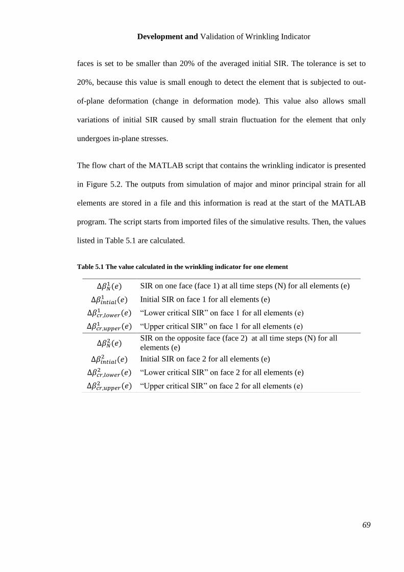
Development and Validation of Wrinkling Indicator
69
faces is set to be smaller than 20% of the averaged initial SIR. The tolerance is set to
20%, because this value is small enough to detect the element that is subjected to out-
of-plane deformation (change in deformation mode). This value also allows small
variations of initial SIR caused by small strain fluctuation for the element that only
undergoes in-plane stresses.
The flow chart of the MATLAB script that contains the wrinkling indicator is presented
in Figure 5.2. The outputs from simulation of major and minor principal strain for all
elements are stored in a file and this information is read at the start of the MATLAB
program. The script starts from imported files of the simulative results. Then, the values
listed in Table 5.1 are calculated.
Table 5.1 The value calculated in the wrinkling indicator for one element
∆𝛽𝑁1(𝑒) SIR on one face (face 1) at all time steps (N) for all elements (e)
∆𝛽𝑖𝑛𝑡𝑖𝑎𝑙1 (𝑒) Initial SIR on face 1 for all elements (e)
∆𝛽𝑐𝑟,𝑙𝑜𝑤𝑒𝑟1 (𝑒) “Lower critical SIR” on face 1 for all elements (e)
∆𝛽𝑐𝑟,𝑢𝑝𝑝𝑒𝑟1 (𝑒) “Upper critical SIR” on face 1 for all elements (e)
∆𝛽𝑁2(𝑒)
SIR on the opposite face (face 2) at all time steps (N) for all
elements (e)
∆𝛽𝑖𝑛𝑡𝑖𝑎𝑙2 (𝑒) Initial SIR on face 2 for all elements (e)
∆𝛽𝑐𝑟,𝑙𝑜𝑤𝑒𝑟2 (𝑒) “Lower critical SIR” on face 2 for all elements (e)
∆𝛽𝑐𝑟,𝑢𝑝𝑝𝑒𝑟2 (𝑒) “Upper critical SIR” on face 2 for all elements (e)
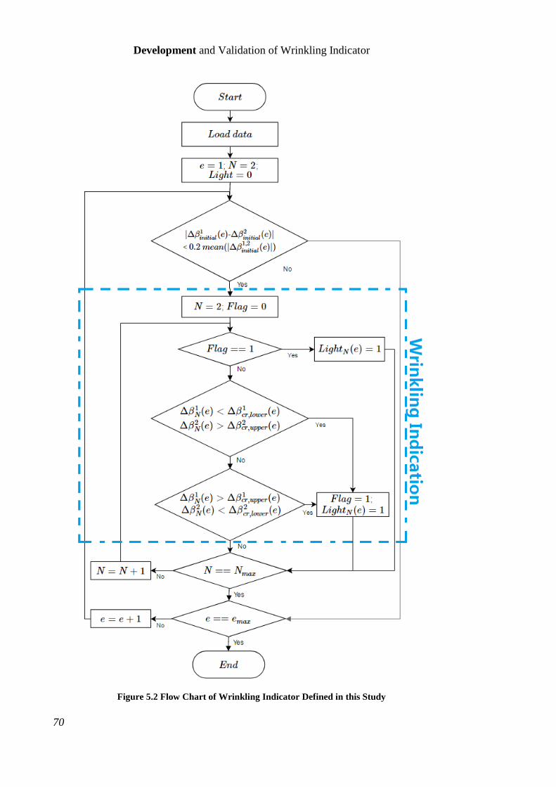
Development and Validation of Wrinkling Indicator
70
Figure 5.2 Flow Chart of Wrinkling Indicator Defined in this Study
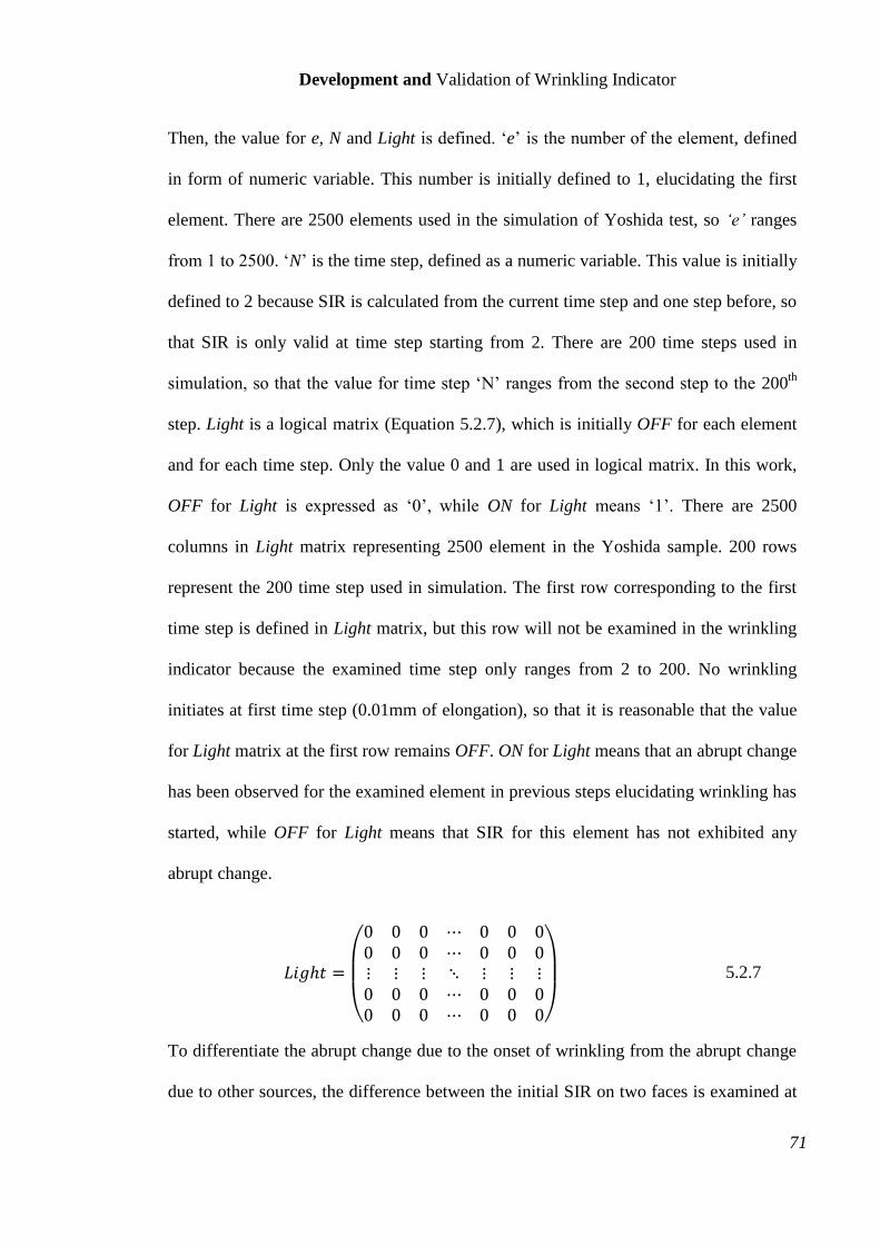
Development and Validation of Wrinkling Indicator
71
Then, the value for e, N and Light is defined. ‘e’ is the number of the element, defined
in form of numeric variable. This number is initially defined to 1, elucidating the first
element. There are 2500 elements used in the simulation of Yoshida test, so ‘e’ ranges
from 1 to 2500. ‘N’ is the time step, defined as a numeric variable. This value is initially
defined to 2 because SIR is calculated from the current time step and one step before, so
that SIR is only valid at time step starting from 2. There are 200 time steps used in
simulation, so that the value for time step ‘N’ ranges from the second step to the 200th
step. Light is a logical matrix (Equation 5.2.7), which is initially OFF for each element
and for each time step. Only the value 0 and 1 are used in logical matrix. In this work,
OFF for Light is expressed as ‘0’, while ON for Light means ‘1’. There are 2500
columns in Light matrix representing 2500 element in the Yoshida sample. 200 rows
represent the 200 time step used in simulation. The first row corresponding to the first
time step is defined in Light matrix, but this row will not be examined in the wrinkling
indicator because the examined time step only ranges from 2 to 200. No wrinkling
initiates at first time step (0.01mm of elongation), so that it is reasonable that the value
for Light matrix at the first row remains OFF. ON for Light means that an abrupt change
has been observed for the examined element in previous steps elucidating wrinkling has
started, while OFF for Light means that SIR for this element has not exhibited any
abrupt change.
𝐿𝑖𝑔ℎ𝑡 =
(
0 0 0 ⋯ 0 0 00 0 0 ⋯ 0 0 0⋮ ⋮ ⋮ ⋱ ⋮ ⋮ ⋮0 0 0 ⋯ 0 0 00 0 0 ⋯ 0 0 0)
5.2.7
To differentiate the abrupt change due to the onset of wrinkling from the abrupt change
due to other sources, the difference between the initial SIR on two faces is examined at
Development and Validation of Wrinkling Indicator
72
each element. When the discrepancy between two values is larger than 20% of the
averaged initial SIR for two faces, the abrupt change in SIR for this element cannot be
attributed to the onset of wrinkling. In this case, the indicator will move to next element
(e=e+1); otherwise the indicator will move to wrinkling indication phase.
In the wrinkling indication phase, the values for time step ‘N’ and a universal logical
variable Flag are firstly defined. Time step ‘N’ is defined to 2 when indicator starts to
examine a new element, so that the indicator checks the abrupt change in SIR from the
first valid value. Flag is a universal logical variable for the simplification of program,
which is switched to OFF when the indicator starts to examine a new element. Flag
turns ON after the first abrupt change in SIR, elucidating the onset of wrinkling. When
the Flag is ON, the Light matrix for this element can be directly switched to ON for the
following time steps, without examining the abrupt change in SIR.
The abrupt change in SIR on two faces behaves differently, so the indications for the
onset of wrinkling are defined through different methods. In this indicator, the face
number (either 1 or 2) is shown as the superscript. Once the SIR (∆𝛽𝑁1(𝑒)) at one
element (e) on face 1 at one time step (N) becomes more negative than the lower critical
SIR on face 1 (∆𝛽𝑐𝑟,𝑙𝑜𝑤𝑒𝑟1 (𝑒)) and SIR at the same element on face 2 becomes less
negative than the upper critical SIR for face 2 (∆𝛽𝑐𝑟,𝑢𝑝𝑝𝑒𝑟2 (𝑒)), the universal variable
Flag and the Light for this step for this element are switched to ON. On the other hand,
if the compression on face 1 is being partially released, Flag and Light will switch ON
when the SIR on this face 1 becomes less negative than the upper critical SIR for face 1
(∆𝛽𝑐𝑟,𝑢𝑝𝑝𝑒𝑟1 (𝑒)) and SIR on face 2 becomes more negative than the lower critical SIR
for face 2 (∆𝛽𝑐𝑟,𝑙𝑜𝑤𝑒𝑟2 (𝑒)). The criteria for two faces are summarized in Table 5.2.
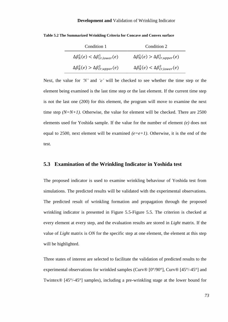
Development and Validation of Wrinkling Indicator
73
Table 5.2 The Summarized Wrinkling Criteria for Concave and Convex surface
Condition 1 Condition 2
∆𝛽𝑁1(𝑒) < ∆𝛽𝑐𝑟,𝑙𝑜𝑤𝑒𝑟
1 (𝑒) ∆𝛽𝑁1(𝑒) > ∆𝛽𝑐𝑟,𝑢𝑝𝑝𝑒𝑟
1 (𝑒)
∆𝛽𝑁2(𝑒) > ∆𝛽𝑐𝑟,𝑢𝑝𝑝𝑒𝑟
2 (𝑒) ∆𝛽𝑁2(𝑒) < ∆𝛽𝑐𝑟,𝑙𝑜𝑤𝑒𝑟
2 (𝑒)
Next, the value for ‘N’ and ‘e’ will be checked to see whether the time step or the
element being examined is the last time step or the last element. If the current time step
is not the last one (200) for this element, the program will move to examine the next
time step (N=N+1). Otherwise, the value for element will be checked. There are 2500
elements used for Yoshida sample. If the value for the number of element (e) does not
equal to 2500, next element will be examined (e=e+1). Otherwise, it is the end of the
test.
5.3 Examination of the Wrinkling Indicator in Yoshida test
The proposed indicator is used to examine wrinkling behaviour of Yoshida test from
simulations. The predicted results will be validated with the experimental observations.
The predicted result of wrinkling formation and propagation through the proposed
wrinkling indicator is presented in Figure 5.5-Figure 5.5. The criterion is checked at
every element at every step, and the evaluation results are stored in Light matrix. If the
value of Light matrix is ON for the specific step at one element, the element at this step
will be highlighted.
Three states of interest are selected to facilitate the validation of predicted results to the
experimental observations for wrinkled samples (Curv® [0°/90°], Curv® [45°/-45°] and
Twintex® [45°/-45°] samples), including a pre-wrinkling stage at the lower bound for
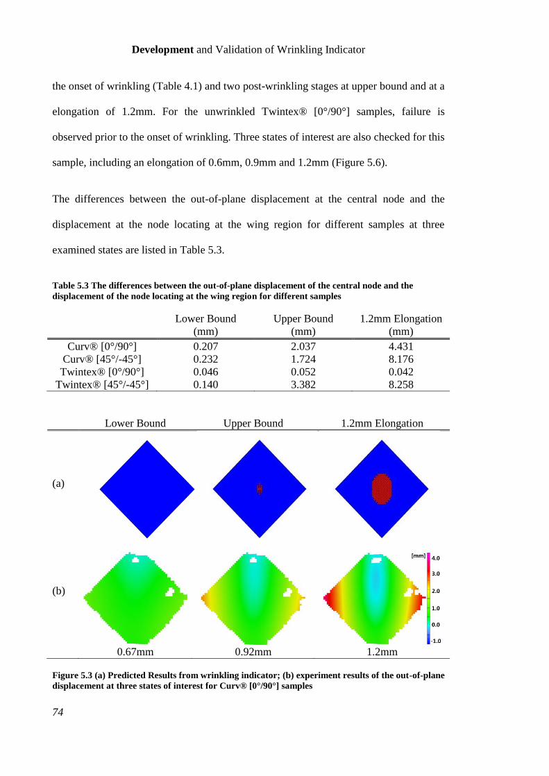
Development and Validation of Wrinkling Indicator
74
the onset of wrinkling (Table 4.1) and two post-wrinkling stages at upper bound and at a
elongation of 1.2mm. For the unwrinkled Twintex® [0°/90°] samples, failure is
observed prior to the onset of wrinkling. Three states of interest are also checked for this
sample, including an elongation of 0.6mm, 0.9mm and 1.2mm (Figure 5.6).
The differences between the out-of-plane displacement at the central node and the
displacement at the node locating at the wing region for different samples at three
examined states are listed in Table 5.3.
Table 5.3 The differences between the out-of-plane displacement of the central node and the
displacement of the node locating at the wing region for different samples
Lower Bound
(mm)
Upper Bound
(mm)
1.2mm Elongation
(mm)
Curv® [0°/90°] 0.207 2.037 4.431
Curv® [45°/-45°] 0.232 1.724 8.176
Twintex® [0°/90°] 0.046 0.052 0.042
Twintex® [45°/-45°] 0.140 3.382 8.258
Lower Bound Upper Bound 1.2mm Elongation
(a)
(b)
0.67mm 0.92mm 1.2mm
Figure 5.3 (a) Predicted Results from wrinkling indicator; (b) experiment results of the out-of-plane
displacement at three states of interest for Curv® [0°/90°] samples
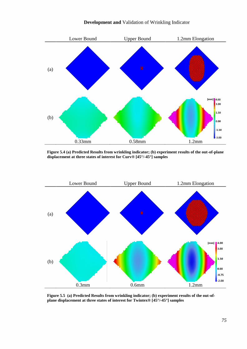
Development and Validation of Wrinkling Indicator
75
Lower Bound Upper Bound 1.2mm Elongation
(a)
(b)
0.33mm 0.58mm 1.2mm
Figure 5.4 (a) Predicted Results from wrinkling indicator; (b) experiment results of the out-of-plane
displacement at three states of interest for Curv® [45°/-45°] samples
Lower Bound Upper Bound 1.2mm Elongation
(a)
(b)
0.3mm 0.6mm 1.2mm
Figure 5.5 (a) Predicted Results from wrinkling indicator; (b) experiment results of the out-of-
plane displacement at three states of interest for Twintex® [45°/-45°] samples
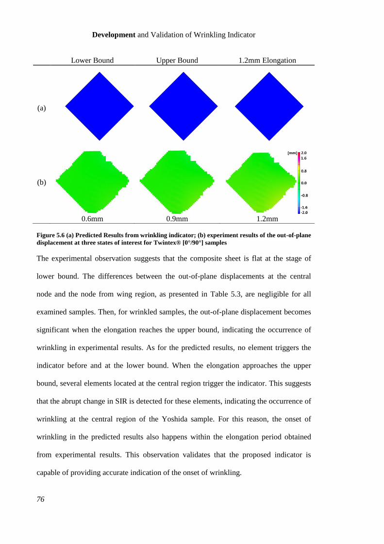
Development and Validation of Wrinkling Indicator
76
Lower Bound Upper Bound 1.2mm Elongation
(a)
(b)
0.6mm 0.9mm 1.2mm
Figure 5.6 (a) Predicted Results from wrinkling indicator; (b) experiment results of the out-of-plane
displacement at three states of interest for Twintex® [0°/90°] samples
The experimental observation suggests that the composite sheet is flat at the stage of
lower bound. The differences between the out-of-plane displacements at the central
node and the node from wing region, as presented in Table 5.3, are negligible for all
examined samples. Then, for wrinkled samples, the out-of-plane displacement becomes
significant when the elongation reaches the upper bound, indicating the occurrence of
wrinkling in experimental results. As for the predicted results, no element triggers the
indicator before and at the lower bound. When the elongation approaches the upper
bound, several elements located at the central region trigger the indicator. This suggests
that the abrupt change in SIR is detected for these elements, indicating the occurrence of
wrinkling at the central region of the Yoshida sample. For this reason, the onset of
wrinkling in the predicted results also happens within the elongation period obtained
from experimental results. This observation validates that the proposed indicator is
capable of providing accurate indication of the onset of wrinkling.
Development and Validation of Wrinkling Indicator
77
Two post-wrinkling stage including the upper bound of the elongation period and the
elongation of 1.2mm are checked to examine the capability of the indicator for
predicting the post-wrinkling behaviour. The experimental results suggest that when the
specimen is being further deformed, wrinkling becomes more severe. A larger
difference between the out-of-plane displacements is obtained at 1.2 mm of elongation
than at the upper bound, showing the propagation of wrinkling, as presented in Table
5.3. With respect to the predicted results, wrinkling grows from a few elements at the
central region to a larger region. This reveals that the proposed indicator also can be
used for describing the wrinkling propagation.
For Twintex® [0°/90°] samples, there is no wrinkling observed in the experiments
before the onset of failure and the difference between the out-of-plane is negligible over
the loading process. Predicted results also suggest no element triggers the wrinkling
indicator, elucidating a good agreement between the predicted results and the
experimental observations. This observation highlights that the proposed indicator can
accurately predict the occurrence of wrinkling.
5.4 Examination of the Wrinkling Indicator in Dome Forming
Wrinkling is a common failure mechanism in sheet forming operations, especially in
dome forming where the samples are not completely constrained at the flange region.
The prime motivation of developing a wrinkling indicator is to be able to detect and in
turn remove wrinkling in forming practises. In this section, the proposed wrinkling
indicator is implemented in dome forming simulations on different samples to test the
validity of the indicator in forming practise and to other class of material. Then, the
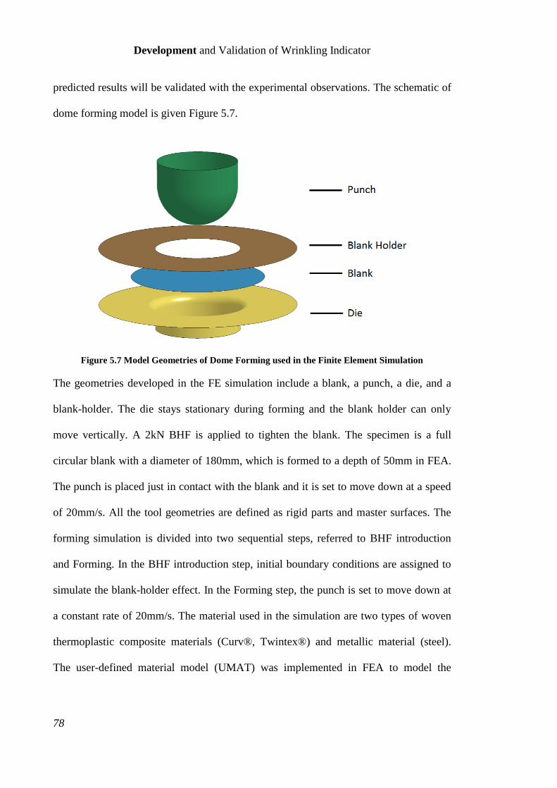
Development and Validation of Wrinkling Indicator
78
predicted results will be validated with the experimental observations. The schematic of
dome forming model is given Figure 5.7.
Figure 5.7 Model Geometries of Dome Forming used in the Finite Element Simulation
The geometries developed in the FE simulation include a blank, a punch, a die, and a
blank-holder. The die stays stationary during forming and the blank holder can only
move vertically. A 2kN BHF is applied to tighten the blank. The specimen is a full
circular blank with a diameter of 180mm, which is formed to a depth of 50mm in FEA.
The punch is placed just in contact with the blank and it is set to move down at a speed
of 20mm/s. All the tool geometries are defined as rigid parts and master surfaces. The
forming simulation is divided into two sequential steps, referred to BHF introduction
and Forming. In the BHF introduction step, initial boundary conditions are assigned to
simulate the blank-holder effect. In the Forming step, the punch is set to move down at
a constant rate of 20mm/s. The material used in the simulation are two types of woven
thermoplastic composite materials (Curv®, Twintex®) and metallic material (steel).
The user-defined material model (UMAT) was implemented in FEA to model the
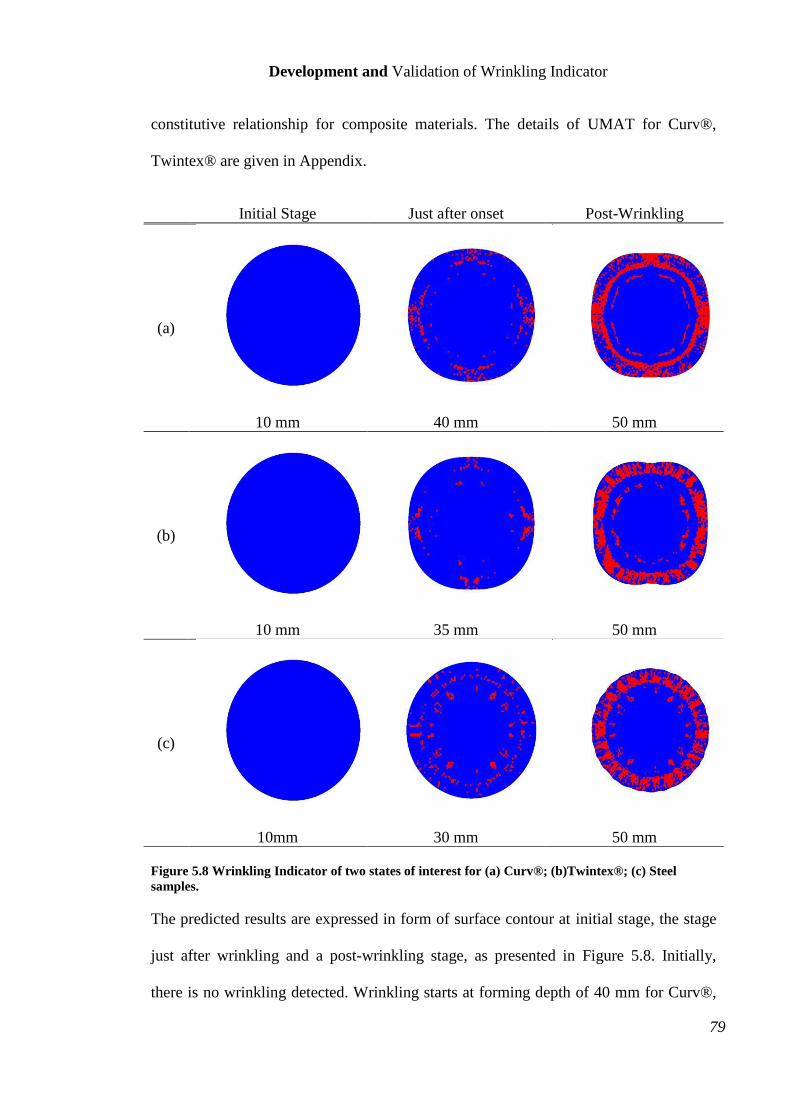
Development and Validation of Wrinkling Indicator
79
constitutive relationship for composite materials. The details of UMAT for Curv®,
Twintex® are given in Appendix.
Initial Stage Just after onset Post-Wrinkling
(a)
10 mm 40 mm 50 mm
(b)
10 mm 35 mm 50 mm
(c)
10mm 30 mm 50 mm
Figure 5.8 Wrinkling Indicator of two states of interest for (a) Curv®; (b)Twintex®; (c) Steel
samples.
The predicted results are expressed in form of surface contour at initial stage, the stage
just after wrinkling and a post-wrinkling stage, as presented in Figure 5.8. Initially,
there is no wrinkling detected. Wrinkling starts at forming depth of 40 mm for Curv®,
Development and Validation of Wrinkling Indicator
80
35mm for Twintex® and 30mm for steel blank. Then, wrinkling grows as the forming
depth increases. When the forming depth reaches 50mm, the predicted result clearly
shows that there is a severe wrinkling occurs on the flange region. For composite
samples, the top view of the shape of the deformed blank appears like a square with
rounded corners. This is due to orthotropic nature of the composite materials caused by
the fibre reinforcement.
Most of the wrinkling in dome forming initiates at the flange regions, which makes
them difficult to observe because the tools (the blank-holder and the die) cover the
flange region during the experiments. For this reason, the predicted results for dome
forming are validated with the formed parts. In dome forming experiments, full circular
blanks with diameter of 180 mm were used. A BHF of 2kN is used and all samples are
formed at a constant punch rate of 20 mm/s to the depth of the onset of wrinkling
suggested by simulation and to the depth of 50mm.
5.4.1 Dome Forming for Curv® Specimens
Figure 5.9 and Figure 5.10 present the predicted results and the formed part of the full
circular Curv® samples. The samples are formed to the depth of 40mm and 50mm.
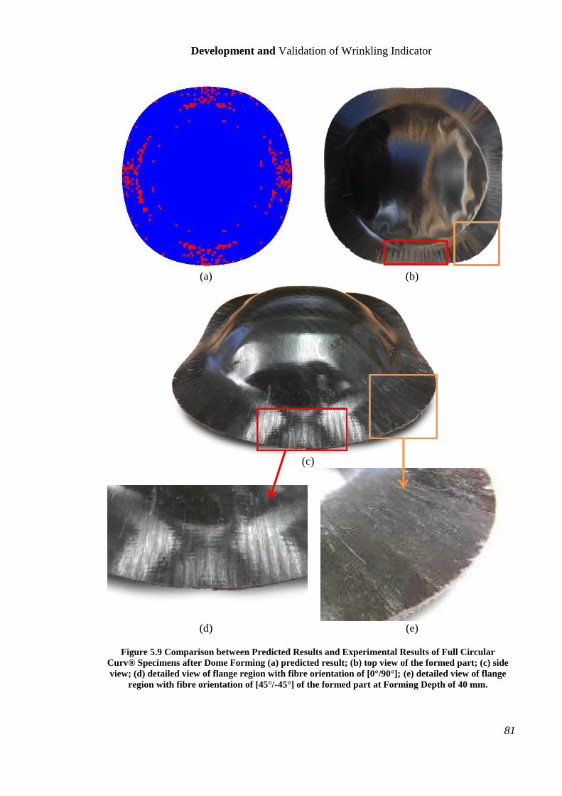
Development and Validation of Wrinkling Indicator
81
(a) (b)
(c)
(d) (e)
Figure 5.9 Comparison between Predicted Results and Experimental Results of Full Circular
Curv® Specimens after Dome Forming (a) predicted result; (b) top view of the formed part; (c) side
view; (d) detailed view of flange region with fibre orientation of [0°/90°]; (e) detailed view of flange
region with fibre orientation of [45°/-45°] of the formed part at Forming Depth of 40 mm.
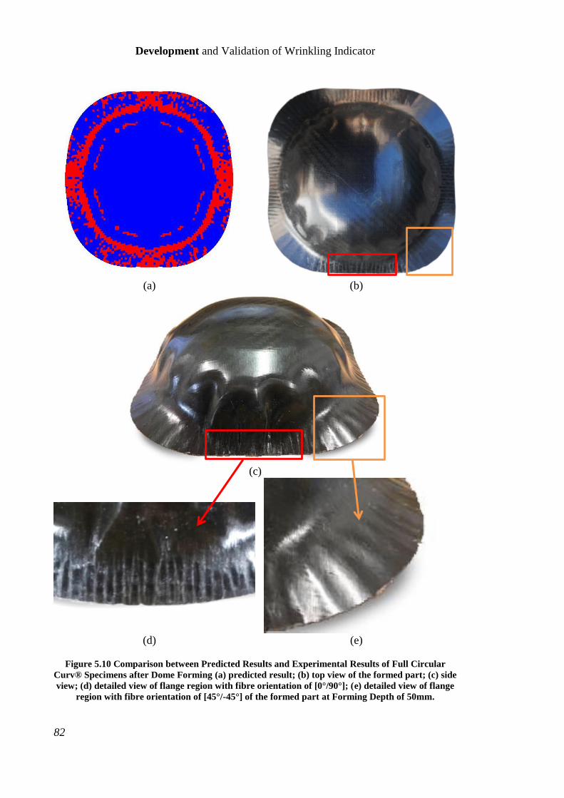
Development and Validation of Wrinkling Indicator
82
(a) (b)
(c)
(d) (e)
Figure 5.10 Comparison between Predicted Results and Experimental Results of Full Circular
Curv® Specimens after Dome Forming (a) predicted result; (b) top view of the formed part; (c) side
view; (d) detailed view of flange region with fibre orientation of [0°/90°]; (e) detailed view of flange
region with fibre orientation of [45°/-45°] of the formed part at Forming Depth of 50mm.
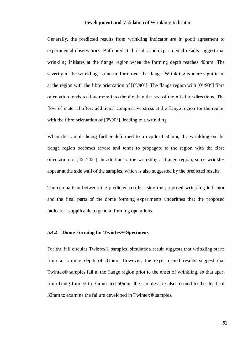
Development and Validation of Wrinkling Indicator
83
Generally, the predicted results from wrinkling indicator are in good agreement to
experimental observations. Both predicted results and experimental results suggest that
wrinkling initiates at the flange region when the forming depth reaches 40mm. The
severity of the wrinkling is non-uniform over the flange. Wrinkling is more significant
at the region with the fibre orientation of [0°/90°]. The flange region with [0°/90°] fibre
orientation tends to flow more into the die than the rest of the off-fibre directions. The
flow of material offers additional compressive stress at the flange region for the region
with the fibre orientation of [0°/90°], leading to a wrinkling.
When the sample being further deformed to a depth of 50mm, the wrinkling on the
flange region becomes severe and tends to propagate to the region with the fibre
orientation of [45°/-45°]. In addition to the wrinkling at flange region, some wrinkles
appear at the side wall of the samples, which is also suggested by the predicted results.
The comparison between the predicted results using the proposed wrinkling indicator
and the final parts of the dome forming experiments underlines that the proposed
indicator is applicable to general forming operations.
5.4.2 Dome Forming for Twintex® Specimens
For the full circular Twintex® samples, simulation result suggests that wrinkling starts
from a forming depth of 35mm. However, the experimental results suggest that
Twintex® samples fail at the flange region prior to the onset of wrinkling, so that apart
from being formed to 35mm and 50mm, the samples are also formed to the depth of
30mm to examine the failure developed in Twintex® samples.
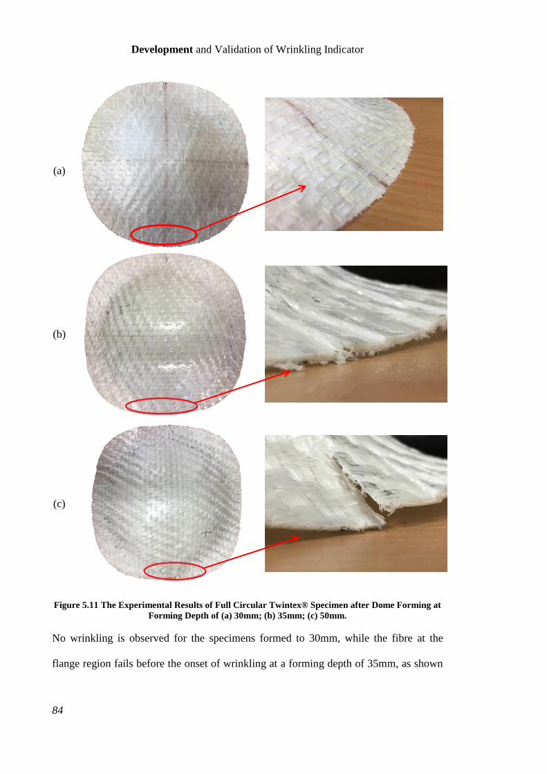
Development and Validation of Wrinkling Indicator
84
(a)
(b)
(c)
Figure 5.11 The Experimental Results of Full Circular Twintex® Specimen after Dome Forming at
Forming Depth of (a) 30mm; (b) 35mm; (c) 50mm.
No wrinkling is observed for the specimens formed to 30mm, while the fibre at the
flange region fails before the onset of wrinkling at a forming depth of 35mm, as shown
Development and Validation of Wrinkling Indicator
85
in Figure 5.11. When the sample was formed to 50mm, the fibre failure then grows
along the radial direction (Figure 5.11). This study focuses only on investigating the
onset of wrinkling and failures, such as fiber fracture, are beyond the scope of this work.
5.4.3 Dome Forming for Steel Specimens
The validity of the proposed indicator is also checked in a sheet metal (steel) dome
forming test, as shown in Figure 5.13. The full circular steel specimen is deformed to
the depth of 30mm and 50mm.
(a) (b)
(c)
Figure 5.12 Comparison between Predicted Results and Experimental Results of Full Circular Steel
Specimen after Dome Forming at Forming Depth of 30 mm (a) predicted result; (b) top view of the
formed part; (c) side view of the formed part.
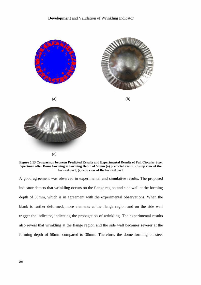
Development and Validation of Wrinkling Indicator
86
(a) (b)
(c)
Figure 5.13 Comparison between Predicted Results and Experimental Results of Full Circular Steel
Specimen after Dome Forming at Forming Depth of 50mm (a) predicted result; (b) top view of the
formed part; (c) side view of the formed part.
A good agreement was observed in experimental and simulative results. The proposed
indicator detects that wrinkling occurs on the flange region and side wall at the forming
depth of 30mm, which is in agreement with the experimental observations. When the
blank is further deformed, more elements at the flange region and on the side wall
trigger the indicator, indicating the propagation of wrinkling. The experimental results
also reveal that wrinkling at the flange region and the side wall becomes severer at the
forming depth of 50mm compared to 30mm. Therefore, the dome forming on steel
Development and Validation of Wrinkling Indicator
87
samples points out that the proposed indicator is capable of predicting the onset and the
growth of wrinkling for metal materials.
5.5 Summary
A wrinkling indicator based on SIR is developed and tested in this chapter. The abrupt
change in SIR only takes place at the onset of wrinkling, but not necessarily at the
wrinkling propagation. To recognize wrinkling at the onset and the growth, the indicator
is defined in such a way that once the onset of wrinkling is detected, the wrinkling
indicator will be turned ON for the following time steps. For this reason, this proposed
wrinkling indicator can detect the onset and the growth of the wrinkling. The
effectiveness of this indicator is validated through Yoshida tests and dome forming tests.
This wrinkling indicator was programmed in MATLAB as a post processing tool from
FEA simulation results. This provides a simulative indicator for onset of wrinkling. By
comparing these results with experimental observations, it is found that the proposed
indicator can predict the region where the wrinkling initiates in different material
systems.

Development and Validation of Wrinkling Indicator
88
Energy Approach of Predicting Wrinkling
89
Chapter 6 Energy Approach of Predicting
Wrinkling
6.1 Introduction
This chapter utilizes the analytical energy method to predict the onset of wrinkling in
Yoshida test. Originally, the analytical energy method was developed to predict the
critical buckling stress. This approach predicts the critical wrinkling load under specific
boundary condition, which describes the overall wrinkling tendency and quantifies the
effect of material properties, boundary conditions and surface deflection at the onset of
wrinkling. In this chapter, this analytical approach is applied at an effective region to
predict the wrinkling instability. The effective region is defined as the region under
compression leading to the localized wrinkling. Since the effective region is the prime
source of the localized wrinkling, the critical wrinkling stress for the effective region
can represent the critical stress for the wrinkling affected region and for the entire
sample.
This chapter will firstly introduce methodology used for the identification of the
effective region and boundary conditions imposed on the effective region. Then, this
method will be implemented in the Yoshida test to estimate the critical stress for
different samples. Finally, a comparison between the predicted, experimental and
simulative results will be presented to validate the usefulness and examine the
limitations of this proposed energy approach.
Energy Approach of Predicting Wrinkling
90
6.2 The Significance of Using Energy Method in Wrinkling Prediction
Though there are numerous attempts in the implementation of energy method into the
wrinkling predication, the methodology used for selecting the wrinkling segment in
these works leads to some difficulties in the critical stress estimation. In literatures, the
typical effective wrinkling region was defined as the segment which is curved into a
half-wave sine curve [33-37]. The width of the effective region is a function of the
wrinkling expansion and the number of waves. In this thesis, a novel approach in the
effective region selection is developed, which is based on the methodology introduced
by Wang and Cao [48]. Wang and Cao suggested that the effective region is the region
under compression leading to the wrinkling at localized region, which is determined
from the simulative stress contour. However, in Wang and Cao’s work [48], there is no
justification on the selection of the effective region and the determination of boundary
condition of the effective region is unclear. In this chapter, FEA results are also
employed in the selection of effective region, but a clear justification on the
determination of effective regions and boundary conditions will be given.
Compared to the conventional methodology for effective region determination
(assuming the segment is curved into specific shape), the calculation procedure for the
critical wrinkling stress in this work is simplified. This is because using the results from
FEA in effective region determination, the effective region determined in this approach
has a constant dimension rather than being a function of the number of waves, so that it
avoids using too many unknowns in the calculation. As a result, using energy approach
associated with this improved effective region selection methodology leads to a faster
Energy Approach of Predicting Wrinkling
91
and simpler approach in the estimation of critical wrinkling stress, compared to the
previous applications in wrinkling predication.
Utilizing energy approach in predicting wrinkling can also provide a direct relationship
between the critical wrinkling stress and material properties, boundary conditions and
geometrical parameters. Having an equation that quantifies the effect of these effective
parameters on the onset of wrinkling is important in the investigation of wrinkling
behaviour. As long as the compressive stress imposed on the effective region is lower
than the estimated critical stress, this region and the entire structure will not exhibit any
wrinkling.
In summary, the combined approach of analytical energy method and numerical method
introduced in this chapter offers a faster and simpler approach in critical wrinkling
stress estimation than the previous applications of energy method.
6.3 Effective Region in Yoshida test
Wang and Cao [48] suggested that the effective region is the dimension undergoing
compression, which is determined from the contour of compressive stress from
simulations. This work stated that the shape of the effective region for Yoshida test is
rectangle, situated at the central of the sample. However, this work failed to justify the
size, shape and location of the effective region and the boundary condition imposed on
this selected region of interest. This section will explain and justify the methodology
used for selecting the effective region and the boundary conditions for the region.
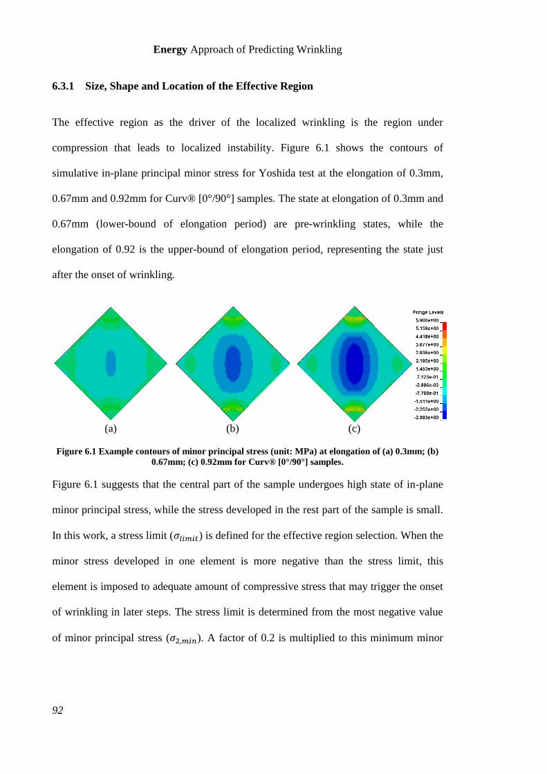
Energy Approach of Predicting Wrinkling
92
6.3.1 Size, Shape and Location of the Effective Region
The effective region as the driver of the localized wrinkling is the region under
compression that leads to localized instability. Figure 6.1 shows the contours of
simulative in-plane principal minor stress for Yoshida test at the elongation of 0.3mm,
0.67mm and 0.92mm for Curv® [0°/90°] samples. The state at elongation of 0.3mm and
0.67mm (lower-bound of elongation period) are pre-wrinkling states, while the
elongation of 0.92 is the upper-bound of elongation period, representing the state just
after the onset of wrinkling.
(a) (b) (c)
Figure 6.1 Example contours of minor principal stress (unit: MPa) at elongation of (a) 0.3mm; (b)
0.67mm; (c) 0.92mm for Curv® [0°/90°] samples.
Figure 6.1 suggests that the central part of the sample undergoes high state of in-plane
minor principal stress, while the stress developed in the rest part of the sample is small.
In this work, a stress limit (𝜎𝑙𝑖𝑚𝑖𝑡) is defined for the effective region selection. When the
minor stress developed in one element is more negative than the stress limit, this
element is imposed to adequate amount of compressive stress that may trigger the onset
of wrinkling in later steps. The stress limit is determined from the most negative value
of minor principal stress (𝜎2,𝑚𝑖𝑛). A factor of 0.2 is multiplied to this minimum minor
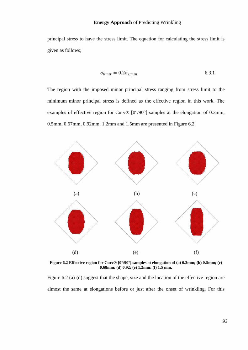
Energy Approach of Predicting Wrinkling
93
principal stress to have the stress limit. The equation for calculating the stress limit is
given as follows;
𝜎𝑙𝑖𝑚𝑖𝑡 = 0.2𝜎2,𝑚𝑖𝑛 6.3.1
The region with the imposed minor principal stress ranging from stress limit to the
minimum minor principal stress is defined as the effective region in this work. The
examples of effective region for Curv® [0°/90°] samples at the elongation of 0.3mm,
0.5mm, 0.67mm, 0.92mm, 1.2mm and 1.5mm are presented in Figure 6.2.
(a) (b) (c)
(d) (e) (f)
Figure 6.2 Effective region for Curv® [0°/90°] samples at elongation of (a) 0.3mm; (b) 0.5mm; (c)
0.68mm; (d) 0.92; (e) 1.2mm; (f) 1.5 mm.
Figure 6.2 (a)-(d) suggest that the shape, size and the location of the effective region are
almost the same at elongations before or just after the onset of wrinkling. For this
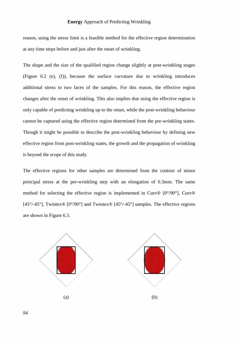
Energy Approach of Predicting Wrinkling
94
reason, using the stress limit is a feasible method for the effective region determination
at any time steps before and just after the onset of wrinkling.
The shape and the size of the qualified region change slightly at post-wrinkling stages
(Figure 6.2 (e), (f)), because the surface curvature due to wrinkling introduces
additional stress to two faces of the samples. For this reason, the effective region
changes after the onset of wrinkling. This also implies that using the effective region is
only capable of predicting wrinkling up to the onset, while the post-wrinkling behaviour
cannot be captured using the effective region determined from the pre-wrinkling states.
Though it might be possible to describe the post-wrinkling behaviour by defining new
effective region from post-wrinkling states, the growth and the propagation of wrinkling
is beyond the scope of this study.
The effective regions for other samples are determined from the contour of minor
principal stress at the pre-wrinkling step with an elongation of 0.3mm. The same
method for selecting the effective region is implemented in Curv® [0°/90°], Curv®
[45°/-45°], Twintex® [0°/90°] and Twintex® [45°/-45°] samples. The effective regions
are shown in Figure 6.3.
(a) (b)
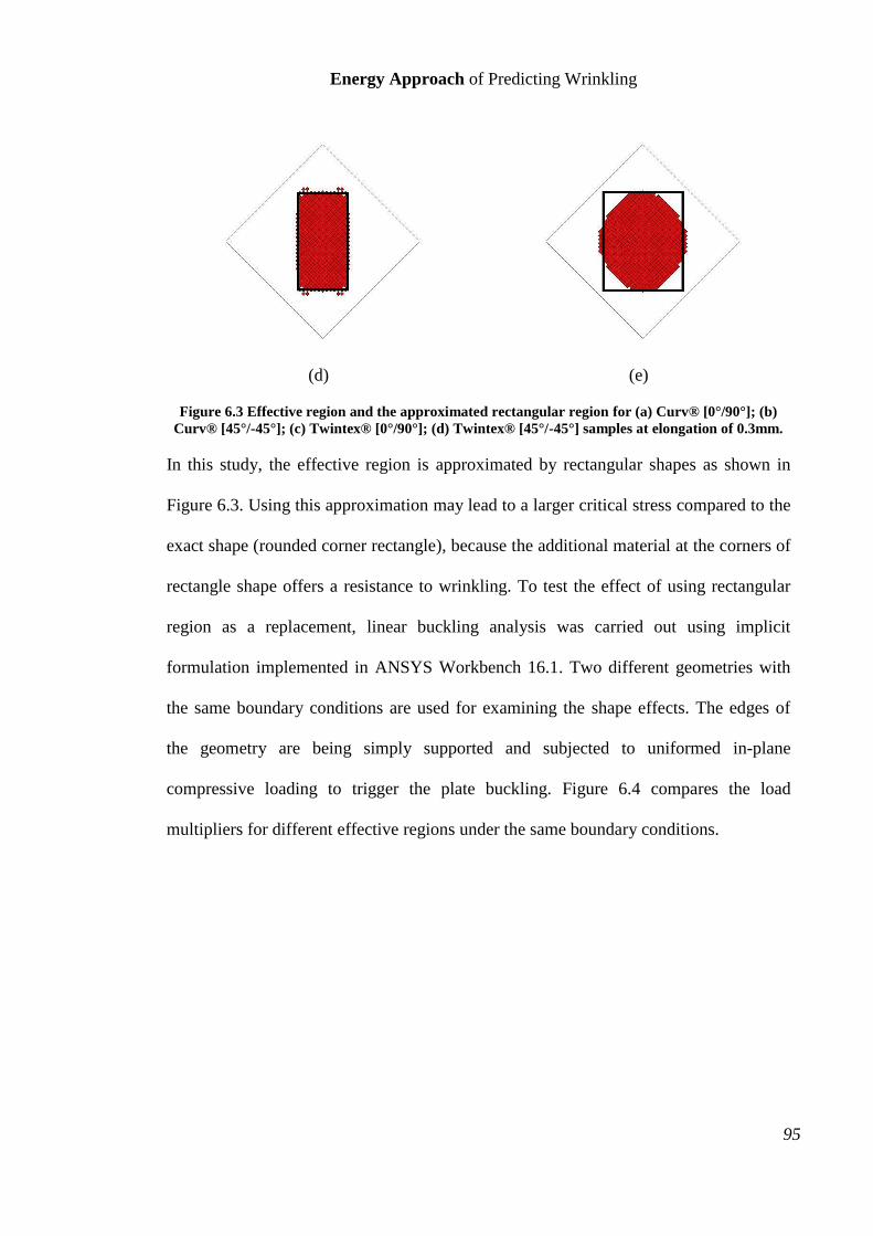
Energy Approach of Predicting Wrinkling
95
(d) (e)
Figure 6.3 Effective region and the approximated rectangular region for (a) Curv® [0°/90°]; (b)
Curv® [45°/-45°]; (c) Twintex® [0°/90°]; (d) Twintex® [45°/-45°] samples at elongation of 0.3mm.
In this study, the effective region is approximated by rectangular shapes as shown in
Figure 6.3. Using this approximation may lead to a larger critical stress compared to the
exact shape (rounded corner rectangle), because the additional material at the corners of
rectangle shape offers a resistance to wrinkling. To test the effect of using rectangular
region as a replacement, linear buckling analysis was carried out using implicit
formulation implemented in ANSYS Workbench 16.1. Two different geometries with
the same boundary conditions are used for examining the shape effects. The edges of
the geometry are being simply supported and subjected to uniformed in-plane
compressive loading to trigger the plate buckling. Figure 6.4 compares the load
multipliers for different effective regions under the same boundary conditions.
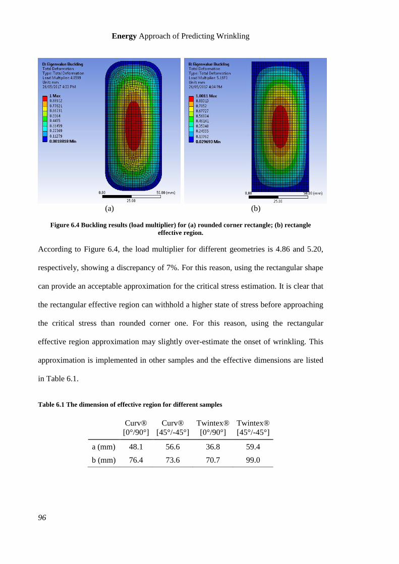
Energy Approach of Predicting Wrinkling
96
(a) (b)
Figure 6.4 Buckling results (load multiplier) for (a) rounded corner rectangle; (b) rectangle
effective region.
According to Figure 6.4, the load multiplier for different geometries is 4.86 and 5.20,
respectively, showing a discrepancy of 7%. For this reason, using the rectangular shape
can provide an acceptable approximation for the critical stress estimation. It is clear that
the rectangular effective region can withhold a higher state of stress before approaching
the critical stress than rounded corner one. For this reason, using the rectangular
effective region approximation may slightly over-estimate the onset of wrinkling. This
approximation is implemented in other samples and the effective dimensions are listed
in Table 6.1.
Table 6.1 The dimension of effective region for different samples
Curv®
[0°/90°]
Curv®
[45°/-45°]
Twintex®
[0°/90°]
Twintex®
[45°/-45°]
a (mm) 48.1 56.6 36.8 59.4
b (mm) 76.4 73.6 70.7 99.0
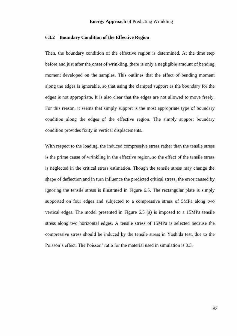
Energy Approach of Predicting Wrinkling
97
6.3.2 Boundary Condition of the Effective Region
Then, the boundary condition of the effective region is determined. At the time step
before and just after the onset of wrinkling, there is only a negligible amount of bending
moment developed on the samples. This outlines that the effect of bending moment
along the edges is ignorable, so that using the clamped support as the boundary for the
edges is not appropriate. It is also clear that the edges are not allowed to move freely.
For this reason, it seems that simply support is the most appropriate type of boundary
condition along the edges of the effective region. The simply support boundary
condition provides fixity in vertical displacements.
With respect to the loading, the induced compressive stress rather than the tensile stress
is the prime cause of wrinkling in the effective region, so the effect of the tensile stress
is neglected in the critical stress estimation. Though the tensile stress may change the
shape of deflection and in turn influence the predicted critical stress, the error caused by
ignoring the tensile stress is illustrated in Figure 6.5. The rectangular plate is simply
supported on four edges and subjected to a compressive stress of 5MPa along two
vertical edges. The model presented in Figure 6.5 (a) is imposed to a 15MPa tensile
stress along two horizontal edges. A tensile stress of 15MPa is selected because the
compressive stress should be induced by the tensile stress in Yoshida test, due to the
Poisson’s effect. The Poisson’ ratio for the material used in simulation is 0.3.
Energy Approach of Predicting Wrinkling
98
(a) (b)
Figure 6.5 Buckling results (load multiplier) for rectangular effective region (a) with a tensile
loading; (b) without tensile loading.
The load multiplier for the rectangular plate with and without a tensile stress is 5.0164
and 5.2154 respectively, so that the critical buckling stress for the plate without a tensile
stress is by 4% higher than the plate under tension. For this reason, it is reasonable to
ignore the tensile effect for the effective region. Ignoring the tensile stress will make the
critical stress estimation slightly higher than the exact value, so that this approximation
again over estimates the wrinkling stress in Yoshida test.
Thus, the wrinkling in the Yoshida test is simplified to the onset of buckling of a
rectangular plate being simply supported along four edges and subjected to a uniform
compressive stress along one pair of edges (𝑥 = 0 𝑎𝑛𝑑 𝑥 = 𝑎), as shown in Figure 6.6.
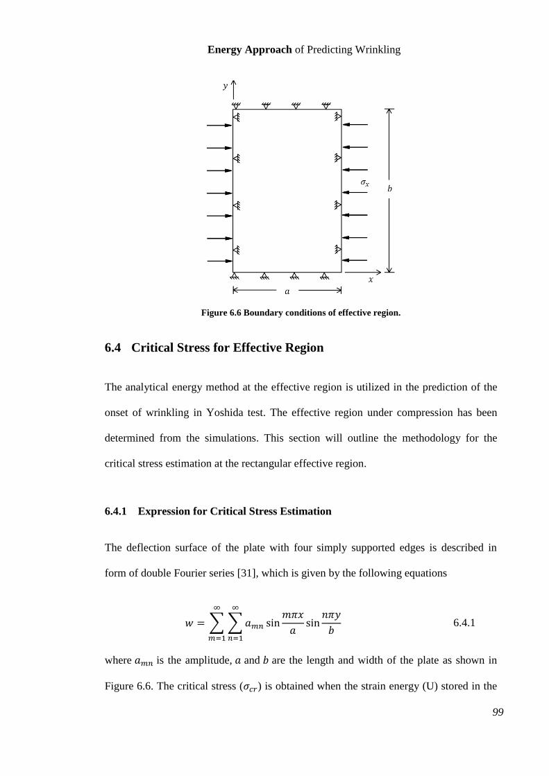
Energy Approach of Predicting Wrinkling
99
Figure 6.6 Boundary conditions of effective region.
6.4 Critical Stress for Effective Region
The analytical energy method at the effective region is utilized in the prediction of the
onset of wrinkling in Yoshida test. The effective region under compression has been
determined from the simulations. This section will outline the methodology for the
critical stress estimation at the rectangular effective region.
6.4.1 Expression for Critical Stress Estimation
The deflection surface of the plate with four simply supported edges is described in
form of double Fourier series [31], which is given by the following equations
𝑤 = ∑ ∑𝑎𝑚𝑛 sin𝑚𝜋𝑥
𝑎sin
𝑛𝜋𝑦
𝑏
∞
𝑛=1
∞
𝑚=1
6.4.1
where 𝑎𝑚𝑛 is the amplitude, 𝑎 and 𝑏 are the length and width of the plate as shown in
Figure 6.6. The critical stress (𝜎𝑐𝑟) is obtained when the strain energy (U) stored in the
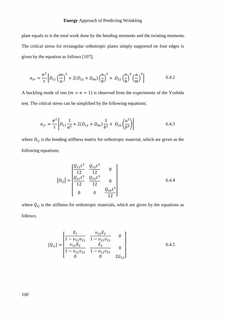
Energy Approach of Predicting Wrinkling
100
plate equals to is the total work done by the bending moments and the twisting moments.
The critical stress for rectangular orthotropic plates simply supported on four edges is
given by the equation as follows [107];
𝜎𝑐𝑟 =𝜋2
𝑡[𝐷11 (
𝑚
𝑎)2
+ 2(𝐷12 + 𝐷66) (𝑛
𝑏)2
+ 𝐷22 (𝑛
𝑏)4
(𝑎
𝑚)2
] 6.4.2
A buckling mode of one (𝑚 = 𝑛 = 1) is observed from the experiments of the Yoshida
test. The critical stress can be simplified by the following equations;
𝜎𝑐𝑟 =𝜋2
𝑡[𝐷11
1
𝑎2+ 2(𝐷12 + 𝐷66)
1
𝑏2+ 𝐷22 (
𝑎2
𝑏4)] 6.4.3
where 𝐷𝑖𝑗 is the bending stiffness matrix for orthotropic material, which are given as the
following equations;
[𝐷𝑖𝑗] =
[ 𝑄11𝑡
3
12
𝑄12𝑡3
120
𝑄21𝑡3
12
𝑄22𝑡3
120
0 0𝑄66𝑡
3
12 ]
6.4.4
where 𝑄𝑖𝑗 is the stiffness for orthotropic materials, which are given by the equations as
follows;
[𝑄𝑖𝑗] =
[
𝐸11 − 𝑣12𝑣21
𝑣12𝐸21 − 𝑣12𝑣21
0
𝑣12𝐸21 − 𝑣12𝑣21
𝐸21 − 𝑣12𝑣21
0
0 0 2𝐺12]
6.4.5
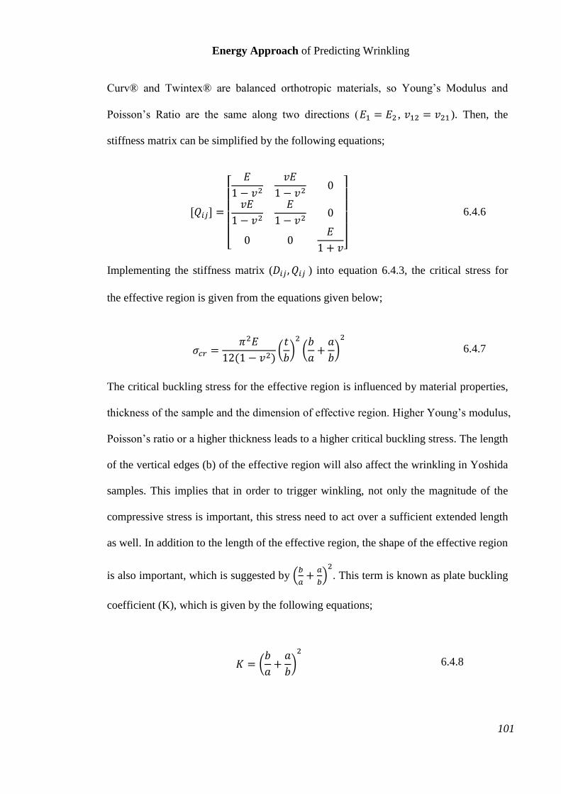
Energy Approach of Predicting Wrinkling
101
Curv® and Twintex® are balanced orthotropic materials, so Young’s Modulus and
Poisson’s Ratio are the same along two directions (𝐸1 = 𝐸2 , 𝑣12 = 𝑣21 ). Then, the
stiffness matrix can be simplified by the following equations;
[𝑄𝑖𝑗] =
[
𝐸
1 − 𝑣2𝑣𝐸
1 − 𝑣20
𝑣𝐸
1 − 𝑣2𝐸
1 − 𝑣20
0 0𝐸
1 + 𝑣]
6.4.6
Implementing the stiffness matrix (𝐷𝑖𝑗 , 𝑄𝑖𝑗 ) into equation 6.4.3, the critical stress for
the effective region is given from the equations given below;
𝜎𝑐𝑟 =𝜋2𝐸
12(1 − 𝑣2)(𝑡
𝑏)2
(𝑏
𝑎+𝑎
𝑏)2
6.4.7
The critical buckling stress for the effective region is influenced by material properties,
thickness of the sample and the dimension of effective region. Higher Young’s modulus,
Poisson’s ratio or a higher thickness leads to a higher critical buckling stress. The length
of the vertical edges (b) of the effective region will also affect the wrinkling in Yoshida
samples. This implies that in order to trigger winkling, not only the magnitude of the
compressive stress is important, this stress need to act over a sufficient extended length
as well. In addition to the length of the effective region, the shape of the effective region
is also important, which is suggested by (𝑏
𝑎+𝑎
𝑏)2
. This term is known as plate buckling
coefficient (K), which is given by the following equations;
𝐾 = (𝑏
𝑎+𝑎
𝑏)2
6.4.8
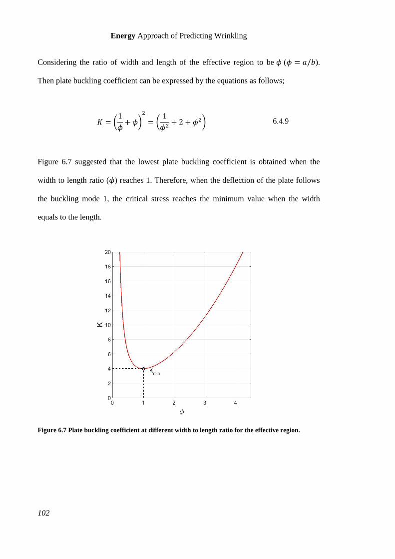
Energy Approach of Predicting Wrinkling
102
Considering the ratio of width and length of the effective region to be 𝜙 (𝜙 = 𝑎/𝑏).
Then plate buckling coefficient can be expressed by the equations as follows;
𝐾 = (1
𝜙+ 𝜙)
2
= (1
𝜙2+ 2 + 𝜙2) 6.4.9
Figure 6.7 suggested that the lowest plate buckling coefficient is obtained when the
width to length ratio (𝜙) reaches 1. Therefore, when the deflection of the plate follows
the buckling mode 1, the critical stress reaches the minimum value when the width
equals to the length.
Figure 6.7 Plate buckling coefficient at different width to length ratio for the effective region.
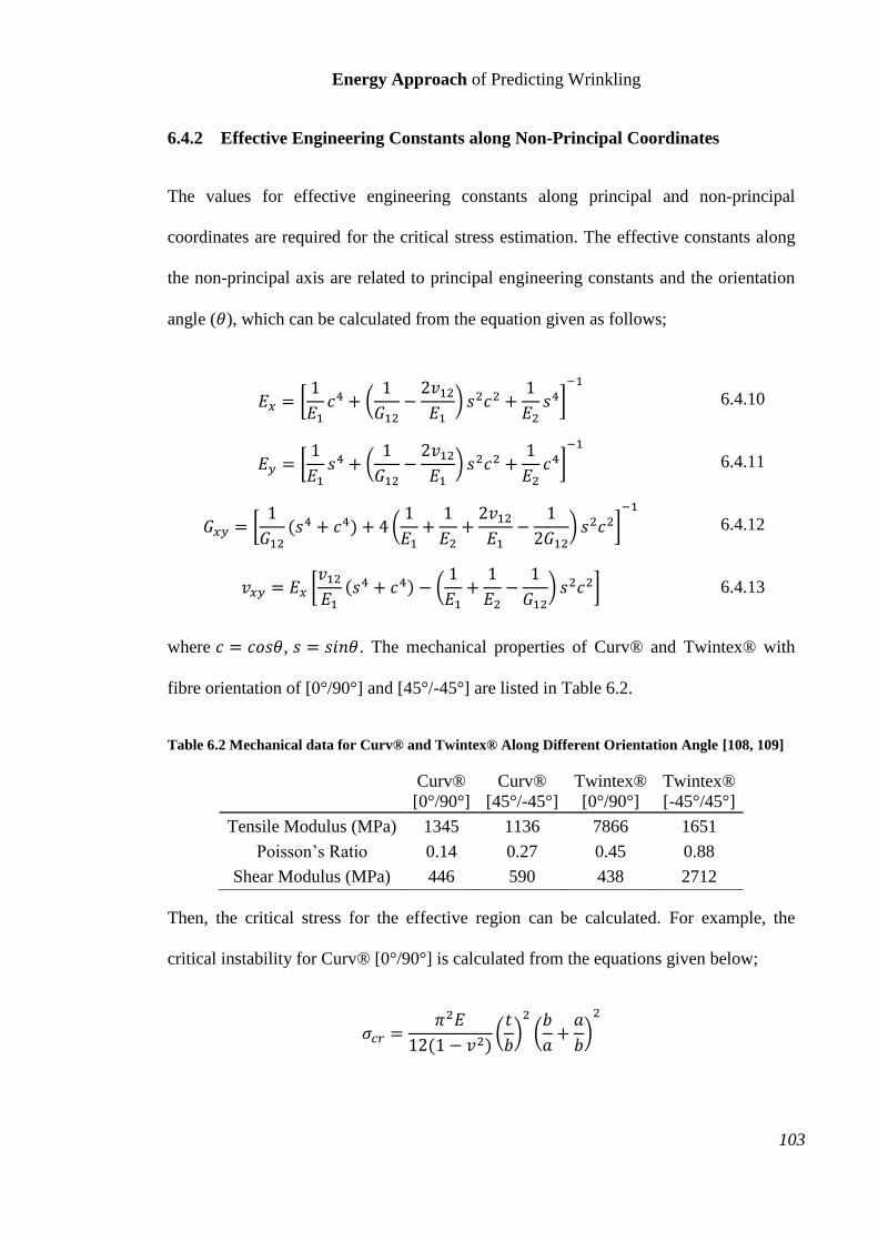
Energy Approach of Predicting Wrinkling
103
6.4.2 Effective Engineering Constants along Non-Principal Coordinates
The values for effective engineering constants along principal and non-principal
coordinates are required for the critical stress estimation. The effective constants along
the non-principal axis are related to principal engineering constants and the orientation
angle (𝜃), which can be calculated from the equation given as follows;
𝐸𝑥 = [1
𝐸1𝑐4 + (
1
𝐺12−2𝑣12𝐸1
) 𝑠2𝑐2 +1
𝐸2𝑠4]
−1
6.4.10
𝐸𝑦 = [1
𝐸1𝑠4 + (
1
𝐺12−2𝑣12𝐸1
) 𝑠2𝑐2 +1
𝐸2𝑐4]
−1
6.4.11
𝐺𝑥𝑦 = [1
𝐺12(𝑠4 + 𝑐4) + 4 (
1
𝐸1+1
𝐸2+2𝑣12𝐸1
−1
2𝐺12) 𝑠2𝑐2]
−1
6.4.12
𝑣𝑥𝑦 = 𝐸𝑥 [𝑣12𝐸1(𝑠4 + 𝑐4) − (
1
𝐸1+1
𝐸2−
1
𝐺12) 𝑠2𝑐2] 6.4.13
where 𝑐 = 𝑐𝑜𝑠𝜃, 𝑠 = 𝑠𝑖𝑛𝜃. The mechanical properties of Curv® and Twintex® with
fibre orientation of [0°/90°] and [45°/-45°] are listed in Table 6.2.
Table 6.2 Mechanical data for Curv® and Twintex® Along Different Orientation Angle [108, 109]
Curv®
[0°/90°]
Curv®
[45°/-45°]
Twintex®
[0°/90°]
Twintex®
[-45°/45°]
Tensile Modulus (MPa) 1345 1136 7866 1651
Poisson’s Ratio 0.14 0.27 0.45 0.88
Shear Modulus (MPa) 446 590 438 2712
Then, the critical stress for the effective region can be calculated. For example, the
critical instability for Curv® [0°/90°] is calculated from the equations given below;
𝜎𝑐𝑟 =𝜋2𝐸
12(1 − 𝑣2)(𝑡
𝑏)2
(𝑏
𝑎+𝑎
𝑏)2
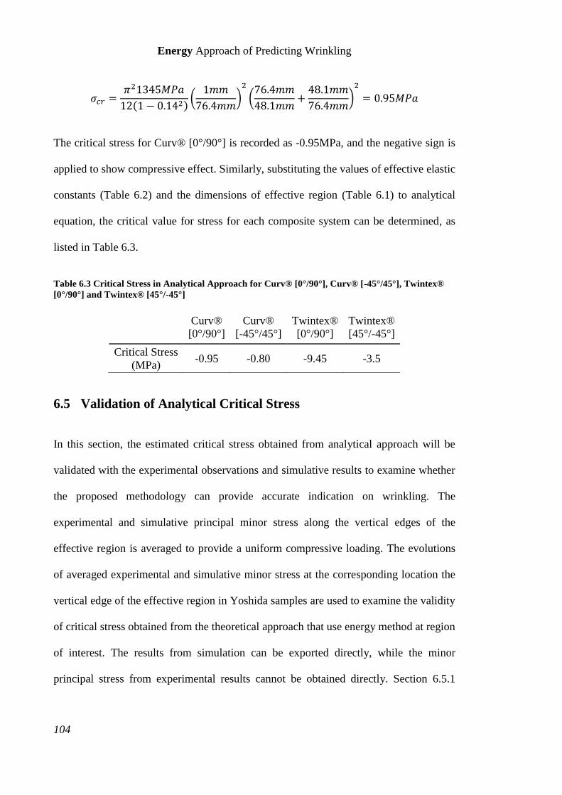
Energy Approach of Predicting Wrinkling
104
𝜎𝑐𝑟 =𝜋21345𝑀𝑃𝑎
12(1 − 0.142)(1𝑚𝑚
76.4𝑚𝑚)2
(76.4𝑚𝑚
48.1𝑚𝑚+48.1𝑚𝑚
76.4𝑚𝑚)2
= 0.95𝑀𝑃𝑎
The critical stress for Curv® [0°/90°] is recorded as -0.95MPa, and the negative sign is
applied to show compressive effect. Similarly, substituting the values of effective elastic
constants (Table 6.2) and the dimensions of effective region (Table 6.1) to analytical
equation, the critical value for stress for each composite system can be determined, as
listed in Table 6.3.
Table 6.3 Critical Stress in Analytical Approach for Curv® [0°/90°], Curv® [-45°/45°], Twintex®
[0°/90°] and Twintex® [45°/-45°]
Curv®
[0°/90°]
Curv®
[-45°/45°]
Twintex®
[0°/90°]
Twintex®
[45°/-45°]
Critical Stress
(MPa) -0.95 -0.80 -9.45 -3.5
6.5 Validation of Analytical Critical Stress
In this section, the estimated critical stress obtained from analytical approach will be
validated with the experimental observations and simulative results to examine whether
the proposed methodology can provide accurate indication on wrinkling. The
experimental and simulative principal minor stress along the vertical edges of the
effective region is averaged to provide a uniform compressive loading. The evolutions
of averaged experimental and simulative minor stress at the corresponding location the
vertical edge of the effective region in Yoshida samples are used to examine the validity
of critical stress obtained from the theoretical approach that use energy method at region
of interest. The results from simulation can be exported directly, while the minor
principal stress from experimental results cannot be obtained directly. Section 6.5.1
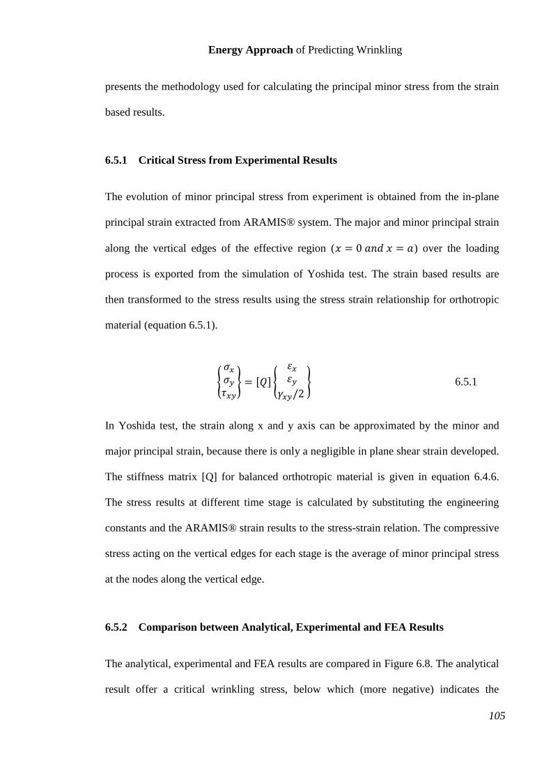
Energy Approach of Predicting Wrinkling
105
presents the methodology used for calculating the principal minor stress from the strain
based results.
6.5.1 Critical Stress from Experimental Results
The evolution of minor principal stress from experiment is obtained from the in-plane
principal strain extracted from ARAMIS® system. The major and minor principal strain
along the vertical edges of the effective region (𝑥 = 0 𝑎𝑛𝑑 𝑥 = 𝑎) over the loading
process is exported from the simulation of Yoshida test. The strain based results are
then transformed to the stress results using the stress strain relationship for orthotropic
material (equation 6.5.1).
{
𝜎𝑥𝜎𝑦𝜏𝑥𝑦
} = [𝑄] {
𝜀𝑥𝜀𝑦
𝛾𝑥𝑦/2 } 6.5.1
In Yoshida test, the strain along x and y axis can be approximated by the minor and
major principal strain, because there is only a negligible in plane shear strain developed.
The stiffness matrix [Q] for balanced orthotropic material is given in equation 6.4.6.
The stress results at different time stage is calculated by substituting the engineering
constants and the ARAMIS® strain results to the stress-strain relation. The compressive
stress acting on the vertical edges for each stage is the average of minor principal stress
at the nodes along the vertical edge.
6.5.2 Comparison between Analytical, Experimental and FEA Results
The analytical, experimental and FEA results are compared in Figure 6.8. The analytical
result offer a critical wrinkling stress, below which (more negative) indicates the
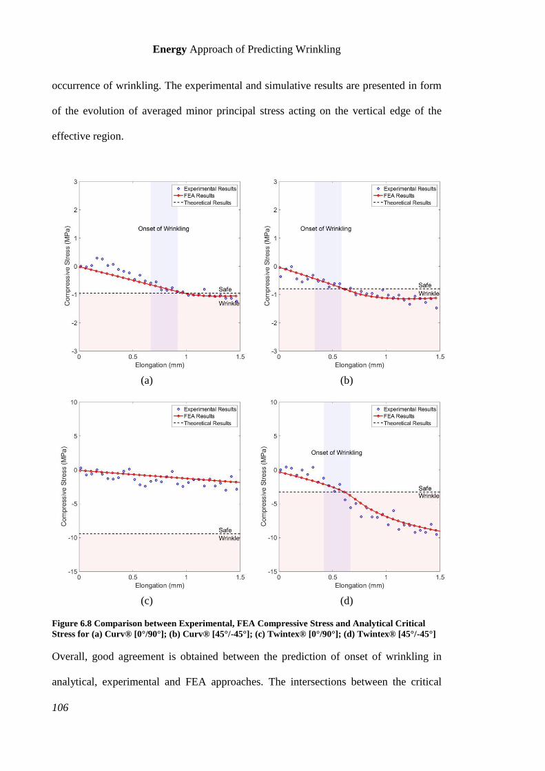
Energy Approach of Predicting Wrinkling
106
occurrence of wrinkling. The experimental and simulative results are presented in form
of the evolution of averaged minor principal stress acting on the vertical edge of the
effective region.
(a) (b)
(c) (d)
Figure 6.8 Comparison between Experimental, FEA Compressive Stress and Analytical Critical
Stress for (a) Curv® [0°/90°]; (b) Curv® [45°/-45°]; (c) Twintex® [0°/90°]; (d) Twintex® [45°/-45°]
Overall, good agreement is obtained between the prediction of onset of wrinkling in
analytical, experimental and FEA approaches. The intersections between the critical
Energy Approach of Predicting Wrinkling
107
wrinkling stress from analytical approach and the stress evolution of experimental and
simulative results illustrate that the onset of wrinkling occurs when the minor principal
stress developed in samples approaches the theoretical critical wrinkling stress. For
wrinkled Curv® [0°/90°], Curv® [45°/-45°] and Twintex® [45°/-45°] samples, the
intersections fall into the elongation region representing the onset of wrinkling observed
in experiments. For Twintex® [0°/90°] samples, the compressive stress from the
experimental and simulative result is much lower than the critical wrinkling stress
estimated from the theoretical method, indicating no wrinkling initiated. These results
indicate that the critical wrinkling stress estimated by the energy method using the
effective region can indicate the onset of wrinkling.
6.6 Summary
In this chapter, the analytical energy method is implemented at an effective region for
the critical wrinkling stress estimation. This effective region is the region under
compression, which is the driver of localized wrinkling; however, there was no clear
definition of the selection of the effective region in the previous studies. This work
introduces a clear methodology for selecting the effective region for Yoshida test, and
this method is likely to be applicable to other wrinkling problems. With a correct
boundary condition assigned to the effective region, the equation for the critical
wrinkling loading can be derived, which quantifies the effect of material properties,
boundary conditions and surface deflection at the onset of wrinkling. Then, the
usefulness of proposed method is validated with the experimental and simulative results
and good agreement is obtained.

Energy Approach of Predicting Wrinkling
108
Conclusion and Recommendations
109
Chapter 7 Conclusion and Recommendations
7.1 Thesis Contribution to knowledge
The approach of using the evolution of the principal strain path to predict the onset of
wrinkling is the fundamental contribution of this study. It was found that the abrupt
change in strain path can indicate the onset of wrinkling. This approach is the first of its
kind in predicting the onset of wrinkling.
SR and SIR are compared for being used as the metric to measure the abrupt change in
strain path. This work clearly demonstrates that current common practise of using SR as
a metric for predicting onset of wrinkling is not robust. The metric of using SIR to
predict the onset of wrinkling can capture more subtle change in strain path, offering
elevated robustness of the indication of the onset of wrinkling. This wrinkling indicator
based on SIR is another contribution of the present work.
A fully automatic wrinkling indicator using the abrupt change in SIR is developed. This
indicator is applicable to predict the onset of wrinkling and the wrinkling propagation in
Yoshida test and dome forming operations. This indicator is also applicable to a variety
of material systems, including but not limit to the composite materials and metallic
materials.
The energy method was used at small wrinkling affected region for the critical
wrinkling stress estimation and good agreement between the simulation and experiment
was obtained. This effective region is defined as the region under compression from the
simulative minor principal stress. The definition of effective region simplifies the usage

Conclusion and Recommendations
110
of energy method compared to conventional energy method application in the literatures.
This work also clarifies a viable methodology for the selection of the size, shape,
orientation and location of effective region, which was not clear in the previous studies.
7.2 Recommendations for future work
This thesis has programmed the wrinkling indicator based on SIR in MATLAB script,
using the information extracted from FEA for predicting wrinkling. In the future, it
would be valuable to develop a user defined loop to implement the indicator in FEA.
The validity of the wrinkling indicator based on SIR is only tested in Yoshida test and
dome forming test. The material systems examined in this work include two fibre
reinforced woven thermoplastic composite material and one metallic material. It seems
to be valuable to further test this indicator to other forming operations and to other
material systems.
The energy approach discussed in Chapter 6 is only applied to Yoshida test. Though a
good agreement is obtained in this study, it is crucial to evaluate the validity of this
approach to other tests. For the test with more complicated geometries, the rectangular
approximation of the shape and the size of the effective region may not valid. In this
case, a two-step implementation can be considered as an alternative for critical stress
estimation. After the identification of the effective region from the primary simulation,
the effective region (irregular) and its boundary conditions can be modelled in FEA to
have the critical wrinkling stress.
Bibliography
111
Chapter 8 Bibliography
[1] Australian Government. (2016). NATIONAL GREENHOUSE ACCOUNTS
FACTORS. Available:
https://www.environment.gov.au/system/files/resources/e30b1895-4870-4a1f-
9b32-3a590de3dddf/files/national-greenhouse-accounts-factors-august-2016.pdf
[2] Climate Action-European Commission. (2017, April). Reducing CO2 emissions
from passenger cars. Available:
https://ec.europa.eu/clima/policies/transport/vehicles/cars_en
[3] S. Birch. (2013). BMW i3, the inside story: what it’s made of, how it’s made.
Available: http://articles.sae.org/12056/
[4] Dry Composites. (2013). BMW i3: first mass produced composite car in
production. Available: http://www.drycomposites.com/bmw-i3-first-mass-
produced-composite-car-in-production/
[5] M. Golzar and M. Poorzeinolabedin, "Prototype fabrication of a composite
automobile body based on integrated structure," The International Journal of
Advanced Manufacturing Technology, vol. 49, pp. 1037-1045, 2010.
[6] B. Lu and N. Wang. (2010). The Boeing 787 Dreamliner, Designing an Aircraft
for the Future. Available: http://www.jyi.org/issue/the-boeing-787-dreamliner-
designing-an-aircraft-for-the-future/
[7] J. Hale. (2006) Boeing 787 from the Ground Up. AERO. Available:
http://www.boeing.com/commercial/aeromagazine/articles/2015_q1/archive.htm
l
[8] P. Brady and M. Brady, "Automotive composites: which way are we going?,"
Reinforced Plastics, vol. 51, pp. 32-35, 2007.
[9] R. Talreja and J. Varna, Modeling Damage, Fatigue and Failure of Composite
Materials: Elsevier, 2015.
[10] A. Derogar and F. Djavanroodi, "Artificial neural network modeling of forming
limit diagram," Materials and Manufacturing Processes, vol. 26, pp. 1415-1422,
2011.
[11] CivilDB. (2011). Buckling Analysis of Tubular Beam Columns. Available:
http://www.civildb.com/buckling-analysis-of-tubular-beam-columns
[12] H. Yang and Y. Lin, "Wrinkling analysis for forming limit of tube bending
processes," Journal of Materials Processing Technology, vol. 152, pp. 363-369,
2004.
Bibliography
112
[13] J. Cao and X. Wang, "An analytical model for plate wrinkling under tri-axial
loading and its application," International Journal of Mechanical Sciences, vol.
42, pp. 617-633, 2000.
[14] J.-B. Kim, D.-Y. Yang, and J. W. Yoon, "Bifurcation Instability of sheet metal
during spring-back," Philosophical magazine, vol. 93, pp. 1914-1935, 2013.
[15] J. Hu, Z. Marciniak, and J. Duncan, Mechanics of sheet metal forming:
Butterworth-Heinemann, 2002.
[16] H. Ameziane-Hassani and K. Neale, "On the analysis of sheet metal wrinkling,"
International journal of mechanical sciences, vol. 33, pp. 13-30, 1991.
[17] Y. Kim and Y. Son, "Study on wrinkling limit diagram of anisotropic sheet
metals," Journal of Materials Processing Technology, vol. 97, pp. 88-94, 2000.
[18] Y. s. Kim, Y. j. Son, and J. y. Park, "Bifurcation analysis of wrinkling formation
for anisotropic sheet," KSME International Journal, vol. 13, pp. 221-228, 1999.
[19] J. Havranek, "Wrinkling limit of tapered pressings," J. Aust. Inst. Met., vol. 20,
pp. 114-119, 1975.
[20] A. Szacinski and P. Thomson, "Investigation of the existence of a wrinkling-
limit curve in plastically-deforming metal sheet," Journal of materials
processing technology, vol. 25, pp. 125-137, 1991.
[21] C. Loganathan and R. Narayanasamy, "Effect of mechanical properties on the
wrinkling behaviour of three different commercially pure aluminium grades
when drawn through conical and tractrix dies," Materials Science and
Engineering: A, vol. 406, pp. 229-253, 2005.
[22] R. Narayanasamy, J. Satheesh, and C. S. Narayanan, "Effect of annealing on
combined forming, fracture and wrinkling limit diagram of Aluminium 5086
alloy sheets," International Journal of Mechanics and Materials in Design, vol.
4, p. 31, 2008.
[23] R. Narayanasamy and C. S. Narayanan, "Forming, fracture and wrinkling limit
diagram for if steel sheets of different thickness," Materials & Design, vol. 29,
pp. 1467-1475, 2008.
[24] R. Narayanasamy, C. Loganathan, and J. Satheesh, "Some study on wrinkling
behaviour of commercially pure aluminium sheet metals of different grades
when drawn through conical and tractrix dies," Materials & Design, vol. 29, pp.
1654-1665, 2008.
[25] H. Li, H. Yang, M. Zhan, and R. Gu, "A new method to accurately obtain
wrinkling limit diagram in NC bending process of thin-walled tube with large
diameter under different loading paths," Journal of Materials Processing
Technology, vol. 177, pp. 192-196, 2006.
Bibliography
113
[26] F. Djavanroodi and A. Derogar, "Experimental and numerical evaluation of
forming limit diagram for Ti6Al4V titanium and Al6061-T6 aluminum alloys
sheets," Materials & Design, vol. 31, pp. 4866-4875, 2010.
[27] N. Akhavan Zanjani, A. Dervaric, and S. Kalyanasundaram, "A Novel Buckling
Indicator using the Correlation Between in-Plane and out-of-Plane
Displacements," 2014.
[28] N. A. Zanjani and S. Kalyanasundaram, "Investigation on the wrinkling limit
diagram of self-reinforced polypropylene woven composite at room
temperature," in Proceedings: the 7th Australasian Congress on Applied
Mechanics (ACAM 7), 9-12 December 2012, the University of Adelaide, North
Terrace Campus/National Committee on Applied Mechanics of Engineers
Australia, 2012, p. 259.
[29] E. Bayraktar, N. Isac, and G. Arnold, "Buckling limit diagrams (BLDs) of
interstitial free steels (IFS): Comparison of experimental and finite element
analysis," Journal of materials processing technology, vol. 164, pp. 1487-1494,
2005.
[30] R. Schleich, C. Albiez, and A. Papaioanu, "Investigation on Simulation of
Buckling of Aluminium Sheet Alloys," in 7th European LS-DYNA Conference,
2009.
[31] H. G. Allen and P. S. Bulson, Background to buckling, 1980.
[32] J. Geckeler, "Plastisches Knicken der Wandung von Hohlzylindern und einige
andere Faltungserscheinungen an Schalen und Blechen," ZAMM‐Journal of
Applied Mathematics and Mechanics/Zeitschrift für Angewandte Mathematik
und Mechanik, vol. 8, pp. 341-352, 1928.
[33] B. W. Senior, "Flange wrinkling in deep-drawing operations," Journal of the
Mechanics and Physics of Solids, vol. 4, pp. 235-246, 1956.
[34] J. Alexander, "An appraisal of the theory of deep drawing," Metallurgical
Reviews, vol. 5, pp. 349-411, 1960.
[35] T. Yu and W. Johnson, "The buckling of annular plates in relation to the deep-
drawing process," International Journal of Mechanical Sciences, vol. 24, pp.
175-188, 1982.
[36] M. Morovvati, B. Mollaei-Dariani, and M. Asadian-Ardakani, "A theoretical,
numerical, and experimental investigation of plastic wrinkling of circular two-
layer sheet metal in the deep drawing," Journal of Materials Processing
Technology, vol. 210, pp. 1738-1747, 2010.
[37] M. R. Morovvati, A. Fatemi, and M. Sadighi, "Experimental and finite element
investigation on wrinkling of circular single layer and two-layer sheet metals in
Bibliography
114
deep drawing process," The International Journal of Advanced Manufacturing
Technology, vol. 54, pp. 113-121, 2011.
[38] L. P. Kollár and G. S. Springer, Mechanics of composite structures: Cambridge
university press, 2003.
[39] A. Agrawal, N. V. Reddy, and P. Dixit, "Determination of optimum process
parameters for wrinkle free products in deep drawing process," Journal of
materials processing technology, vol. 191, pp. 51-54, 2007.
[40] A. Agrawal, N. V. Reddy, and P. Dixit, "Optimal blank shape prediction
considering sheet thickness variation: an upper bound approach," journal of
materials processing technology, vol. 196, pp. 249-258, 2008.
[41] N. Kawai, "Critical Conditions of Wrinkling in Deep Drawing of Sheet Metals:
1 st Report, Fundamentals of Analysis and Results in Case where a Blank-
Holder is not Used," Bulletin of JSME, vol. 4, pp. 169-175, 1961.
[42] K. Zheng, D. J. Politis, J. Lin, and T. A. Dean, "A study on the buckling
behaviour of aluminium alloy sheet in deep drawing with macro-textured
blankholder," International Journal of Mechanical Sciences, vol. 110, pp. 138-
150, 2016.
[43] A. Brosius and A. Mousavi, "Lubricant free deep drawing process by macro
structured tools," CIRP Annals-Manufacturing Technology, vol. 65, pp. 253-256,
2016.
[44] Q. Kong, Z. Yu, Y. Zhao, H. Wang, and Z. Lin, "Theoretical prediction of
flange wrinkling in first-pass conventional spinning of hemispherical part,"
Journal of Materials Processing Technology, vol. 246, pp. 56-68, 2017.
[45] J. Cao and M. Boyce, "Wrinkling behavior of rectangular plates under lateral
constraint," International journal of solids and structures, vol. 34, pp. 153-176,
1997.
[46] X. Wang and J. Cao, "An analytical prediction of flange wrinkling in sheet metal
forming," Journal of Manufacturing Processes, vol. 2, pp. 100-107, 2000.
[47] J. Cao, A. Karafillis, and M. Ostrowski, "Prediction of flange wrinkles in deep
drawing," Studies in applied mechanics, vol. 45, pp. 301-310, 1997.
[48] X. Wang and J. Cao, "On the prediction of side-wall wrinkling in sheet metal
forming processes," International Journal of Mechanical Sciences, vol. 42, pp.
2369-2394, 2000.
[49] J. Cao, "Prediction of plastic wrinkling using the energy method,"
TRANSACTIONS-AMERICAN SOCIETY OF MECHANICAL ENGINEERS
JOURNAL OF APPLIED MECHANICS, vol. 66, pp. 646-652, 1999.
Bibliography
115
[50] H. Lu, H. S. Cheng, J. Cao, and W. K. Liu, "Adaptive enrichment meshfree
simulation and experiment on buckling and post-buckling analysis in sheet metal
forming," Computer Methods in Applied Mechanics and Engineering, vol. 194,
pp. 2569-2590, 2005.
[51] M. A. Shafaat, M. Abbasi, and M. Ketabchi, "Investigation into wall wrinkling
in deep drawing process of conical cups," Journal of Materials Processing
Technology, vol. 211, pp. 1783-1795, 2011.
[52] X. Wang and J. Cao, "Wrinkling limit in tube bending," TRANSACTIONS-
AMERICAN SOCIETY OF MECHANICAL ENGINEERS JOURNAL OF
ENGINEERING MATERIALS AND TECHNOLOGY, vol. 123, pp. 430-435,
2001.
[53] R. F. Gibson, Principles of composite material mechanics: CRC press, 2016.
[54] Fiberforge. (2017, April). Thermoplastic Composite Materials. Available:
http://www.fiberforge.com/thermoplastic-composites/thermoplastic-
composites.php
[55] M. J. Turner, "Stiffness and deflection analysis of complex structures," journal
of the Aeronautical Sciences, 2012.
[56] S. Kalpakjian, S. R. Schmid, and K. V. Sekar, Manufacturing engineering and
technology: Pearson Upper Saddle River, NJ, USA, 2014.
[57] N. Cabrera, "Recyclable all-polypropylene composites: concept, properties and
manufacturing," 2004.
[58] J. Newman. (2015). Woven Fabric; Simple Structures. Available:
https://www.humphriesweaving.co.uk/woven-fabric-structure/
[59] E. Haque. (2015). Comprehensive Study on Twill Weave. Available:
http://textilelearner.blogspot.com.au/2015/06/comprehensive-study-on-twill-
weave.html
[60] textile school. (2017, April). Twill Weaves Available:
http://www.textileschool.com/articles/125/twill-weaves
[61] S. Venkatesan, "Stamp Forming of Composite Materials: An Experimental and
Analytical Study," PhD Thesis, The Australian National University, 2012.
[62] G. Dhatt, E. Lefrançois, and G. Touzot, Finite element method: John Wiley &
Sons, 2012.
[63] L. Martinez. (2014). Thermoset and Thermoplastic Composites; What’s the
Difference? Available: http://www.instron.com.au/en-au/our-company/press-
room/blog/2014/april/thermoset-and-thermoplastic-composites-what-is-the-
difference
Bibliography
116
[64] T. Peijs, "Composites for recyclability," Materials today, vol. 6, pp. 30-35, 2003.
[65] A. N. Netravali and S. Chabba, "Composites get greener," Materials today, vol.
6, pp. 22-29, 2003.
[66] D. Hourston and J. Brysdon, "Degradation of Plastics and Polymers," Shreir's
Corrosion, vol. 3, pp. 2369-2386, 2010.
[67] C. Maier and T. Calafut, Polypropylene: the definitive user's guide and databook:
William Andrew, 1998.
[68] Makeitfrom. (2016). Polyetheretherketone (PEEK). Available:
http://www.makeitfrom.com/material-properties/Polyetheretherketone-PEEK
[69] S. G. Advani and K. T. Hsiao, Manufacturing techniques for polymer matrix
composites (PMCs): Elsevier, 2012.
[70] P. K. Mallick, Fiber-reinforced composites: materials, manufacturing, and
design: CRC press, 2007.
[71] N. Zanjani and S. Kalyanasundaram, "Stretch Forming Simulation of Woven
Composites Based on an Orthotropic Non-Linear Material Model," Journal of
Materials Science and Chemical Engineering, vol. 3, p. 168, 2015.
[72] Á. Kmetty, T. Bárány, and J. Karger-Kocsis, "Self-reinforced polymeric
materials: a review," Progress in Polymer Science, vol. 35, pp. 1288-1310, 2010.
[73] Composite World. (2012). Hockey equipment manufacturer chooses patented
CURV self-reinforced thermoplastic for elite skates. Available:
http://www.compositesworld.com/news/propex-to-supply-curv-composite-
technology-to-bauer-for-hockey-skates
[74] FILMEDIA EVERSPRING. (2016). FILTER FABRIC WEAVE SELECTION.
Available: http://best-filter.com/filter-fabric-weave-selection/
[75] Fibre2fashion. (2017, April). Different Types Of Weaves. Available:
http://www.fibre2fashion.com/industry-article/3343/different-types-of-
weaves?page=1
[76] D. Puglia, J. Biagiotti, and J. Kenny, "A review on natural fibre-based
composites—Part II: Application of natural reinforcements in composite
materials for automotive industry," Journal of Natural Fibers, vol. 1, pp. 23-65,
2005.
[77] B. Alcock, N. Cabrera, N. M. Barkoula, J. Loos, and T. Peijs, "Interfacial
properties of highly oriented coextruded polypropylene tapes for the creation of
recyclable all polypropylene composites," Journal of Applied Polymer Science,
vol. 104, pp. 118-129, 2007.
Bibliography
117
[78] J. Chen, C. Wu, F. Pu, and C. Chiu, "Fabrication and mechanical properties of
self-reinforced poly (ethylene terephthalate) composites," structure, vol. 30, p.
31, 2011.
[79] C. Gao, L. Yu, H. Liu, and L. Chen, "Development of self-reinforced polymer
composites," Progress in Polymer Science, vol. 37, pp. 767-780, 2012.
[80] Owens Corning. (2006). TWINTEX® Glass Fabrics product information.
Available:
http://www.ocvreinforcements.com/pdf/products/Twintex_TPP_09_2008_Rev0.
[81] W. Hufenbach, R. Böhm, M. Thieme, A. Winkler, E. Mäder, J. Rausch, et al.,
"Polypropylene/glass fibre 3D-textile reinforced composites for automotive
applications," Materials & Design, vol. 32, pp. 1468-1476, 2011.
[82] C. Lynam and A. S. Milani, A Guide to Modeling Thermoplastic Composite
Manufacturing Processes, 2015.
[83] B. Choi, O. Diestel, and P. Offermann, "Commingled CF/PEEK hybrid yarns for
use in textile reinforced high performance rotors," in 12th international
conference on composite materials (ICCM), Paris, 1999.
[84] Spe, SPE/ANTEC 1997 Proceedings: CRC Press 1997.
[85] K. Yoshida, "Purpose and Feature of Yoshida Buckling Test," J. Jpn. Soc.
Technol. Plast, vol. 24, pp. 901-903, 1983.
[86] H. Cheng, J. Cao, H. Yao, S. Liu, and B. Kinsey, "Wrinkling behavior of
laminated steel sheets," Journal of Materials Processing Technology, vol. 151,
pp. 133-140, 2004.
[87] A. Szacinski and P. Thomson, "The effect of mechanical properties on the
wrinkling behaviour of sheet materials in the yoshida test," Journal of
mechanical working technology, vol. 10, pp. 87-102, 1984.
[88] A. Mamalis, L. Hatzikonstantis, and Z. Marciniak, "On the Yoshida Buckling
Test of High Strength and Coated Low Carbon Steels," CIRP Annals-
Manufacturing Technology, vol. 36, pp. 185-189, 1987.
[89] J. Kim, J. Yoon, and D. Yang, "Wrinkling initiation and growth in modified
Yoshida buckling test: finite element analysis and experimental comparison,"
International journal of mechanical sciences, vol. 42, pp. 1683-1714, 2000.
[90] N. Akhavan Zanjani and S. Kalyanasundaram, "Wrinkling phenomenon during
uniaxial extension of a woven thermoplastic composite," 2015.
[91] N. Akhavan Zanjani, A. Dervaric, and S. Kalyanasundaram, "A Novel Buckling
Indicator using the Correlation Between in-Plane and out-of-Plane
Displacements," 2014.
Bibliography
118
[92] GOM Optical Measuring Techniques, "Aramis v5. 4. 1 user manual," GOM
mbH, 2005.
[93] GOM Optical Measuring Techniques, "Aramis v6. 1 user manual," GOM mbH,
2009.
[94] GOM Optical Measuring Techniques, "Aramis User information - Hardward-
Sensor Configuration Examples," GOM mbH, 2011.
[95] H. Andersen, J. Casal, A. Dandrieux, B. Debray, V. De Dianous, N. Duijm, et
al., "ARAMIS user guide," The European Commission Community Research,
2004.
[96] J. O. Hallquist, "LS-DYNA theory manual," Livermore software technology
corporation, vol. 3, pp. 25-31, 2006.
[97] O. Zienkiewicz and R. Taylor, "The finite element method, Butterworth
Heinemann," ed: USA, 2000.
[98] J.-B. Kim, D.-Y. Yang, J.-W. Yoon, and F. Barlat, "The effect of plastic
anisotropy on compressive instability in sheet metal forming," International
Journal of Plasticity, vol. 16, pp. 649-676, 2000.
[99] J. O. Hallquist, "LS-DYNA keyword user’s manual," Livermore Software
Technology Corporation, vol. 970, 2007.
[100] A. Haufe, K. Schweizerhof, and P. DuBois, "Properties & Limits: Review of
Shell Element Formulations," Dynamore2013.
[101] B. T. Astrom, Manufacturing of polymer composites: CRC Press, 1997.
[102] ANSYS User's Manual, "Structural analysis guide," ANSYS Inc, 1998.
[103] E. Lindgaard, E. Lund, and K. Rasmussen, "Nonlinear buckling optimization of
composite structures considering “worst” shape imperfections," International
Journal of Solids and Structures, vol. 47, pp. 3186-3202, 2010.
[104] E. Lindgaard and E. Lund, "Nonlinear buckling optimization of composite
structures," Computer methods in applied mechanics and engineering, vol. 199,
pp. 2319-2330, 2010.
[105] N. Kristanič and J. Korelc, "Optimization method for the determination of the
most unfavorable imperfection of structures," Computational Mechanics, vol. 42,
pp. 859-872, 2008.
[106] N. Liu, H. Yang, H. Li, Z. Tao, and X. Hu, "An imperfection-based perturbation
method for plastic wrinkling prediction in tube bending under multi-die
constraints," International Journal of Mechanical Sciences, vol. 98, pp. 178-194,
2015.

Bibliography
119
[107] R. M. Jones, Mechanics of composite materials vol. 193: Scripta Book Company
Washington, DC, 1975.
[108] OCV Reforcements. (2008). TWINTEX® PP GLass Fabrics product
information. Available: http://pdf.nauticexpo.com/pdf/vetrotex-ocv-
reinforcements/twintex-r-pp/27891-12919.html
[109] L. Mosse, "The development of a finite element model for simulating the stamp
forming of fibre-metal laminates.," PhD Thesis, The Australian National
University, 2006.

Bibliography
120
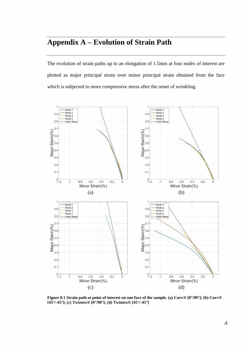
A
Appendix A – Evolution of Strain Path
The evolution of strain paths up to an elongation of 1.5mm at four nodes of interest are
plotted as major principal strain over minor principal strain obtained from the face
which is subjected to more compressive stress after the onset of wrinkling.
(a) (b)
(c) (d)
Figure 8.1 Strain path at point of interest on one face of the sample. (a) Curv® [0°/90°]; (b) Curv®
[45°/-45°]; (c) Twintex® [0°/90°]; (d) Twintex® [45°/-45°]
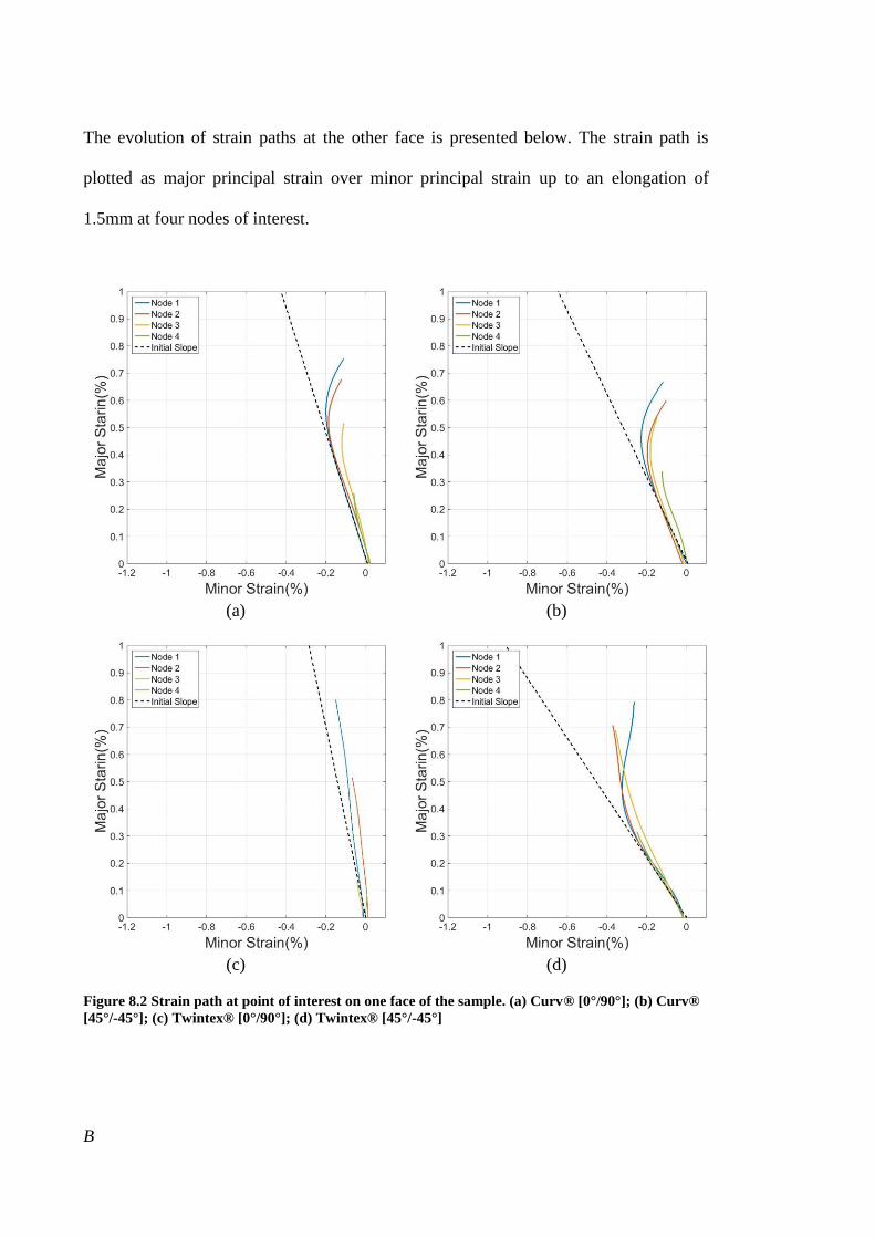
B
The evolution of strain paths at the other face is presented below. The strain path is
plotted as major principal strain over minor principal strain up to an elongation of
1.5mm at four nodes of interest.
(a) (b)
(c) (d)
Figure 8.2 Strain path at point of interest on one face of the sample. (a) Curv® [0°/90°]; (b) Curv®
[45°/-45°]; (c) Twintex® [0°/90°]; (d) Twintex® [45°/-45°]
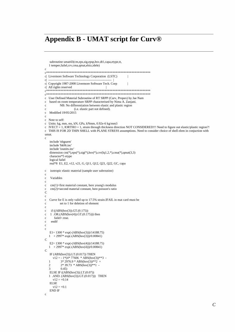
C
Appendix B - UMAT script for Curv®
subroutine umat43(cm,eps,sig,epsp,hsv,dt1,capa,etype,tt, 1 temper,failel,crv,cma,qmat,elsiz,idele)
c
c****************************************************************** c| Livermore Software Technology Corporation (LSTC) |
c| ------------------------------------------------------------ |
c| Copyright 1987-2008 Livermore Software Tech. Corp | c| All rights reserved |
c******************************************************************
c****************************************************************** c User Defined Material Subroutine of RT SRPP (Curv, Propex) by Jae Nam
c based on room temperature SRPP characterised by Nima A. Zanjani.
c NB: No differentiation between elastic and plastic region c (i.e. elastic part not defined).
c Modified 19/05/2015
c c Note to self:
c Units: kg, mm, ms, kN, GPa, kNmm, 0.92e-6 kg/mm3 c IVECT = 1, IORTHO = 1, strain through thickness direction NOT CONSIDERED!!! Need to figure out elastic/plastic region?!
c THIS IS FOR 2D THIN SHELL with PLANE STRESS assumptions. Need to consider choice of shell elem in conjuction with
umat. c
include 'nlqparm'
include 'bk06.inc' include 'iounits.inc'
dimension cm(*),eps(*),sig(*),hsv(*),crv(lq1,2,*),cma(*),qmat(3,3)
character*5 etype logical failel
real*8 E1, E2, v12, v21, G, Q11, Q12, Q21, Q22, GC, capa
c isotropic elastic material (sample user subroutine)
c
c Variables c
c cm(1)=first material constant, here young's modulus
c cm(2)=second material constant, here poisson's ratio C
c
c Curve for E is only valid up to 17.5% strain.IFAIL in mat card must be c set to 1 for deletion of element
c
c if ((ABS(hsv(3)).GT.(0.175)) c 1 .OR.(ABS(hsv(4)).GT.(0.175))) then
c failel=.true.
c endif c
c
E1= 1300 * exp(-(ABS(hsv(3)))/14188.75) 1 + 2997* exp(-(ABS(hsv(3)))/0.00841)
C
E2= 1300 * exp(-(ABS(hsv(4)))/14188.75)
1 + 2997* exp(-(ABS(hsv(4)))/0.00841)
C
IF (ABS(hsv(3)).LT.(0.017)) THEN v12 = - 1*(4* 77606 * ABS(hsv(3))**3 -
1 3* 2976.9 * ABS(hsv(3))**2 +
2 2* 39.73 * ABS(hsv(3))**1 - 3 0.45)
ELSE IF ((ABS(hsv(3)).LT.(0.07))
1 .AND. (ABS(hsv(3)).GT.(0.017))) THEN v12 = +0.14
ELSE
v12 = +0.1 END IF
c
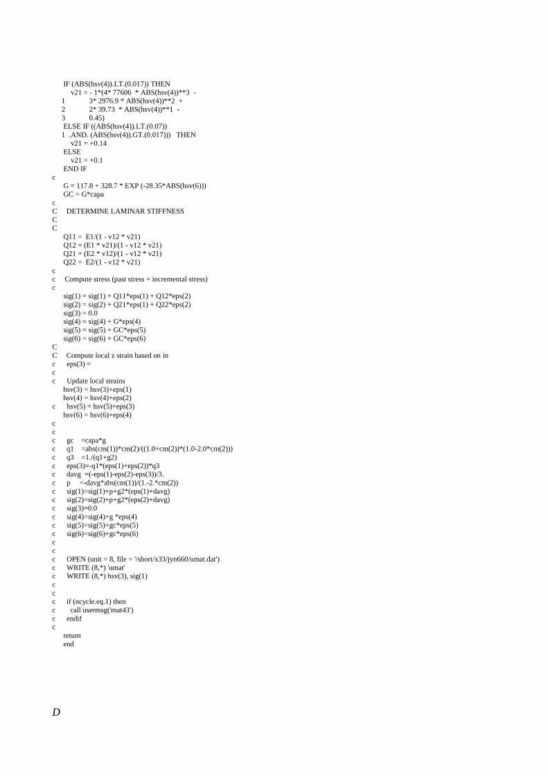
D
IF (ABS(hsv(4)).LT.(0.017)) THEN
v21 = - 1*(4* 77606 * ABS(hsv(4))**3 - 1 3* 2976.9 * ABS(hsv(4))**2 +
2 2* 39.73 * ABS(hsv(4))**1 -
3 0.45) ELSE IF ((ABS(hsv(4)).LT.(0.07))
1 .AND. (ABS(hsv(4)).GT.(0.017))) THEN
v21 = +0.14 ELSE
v21 = +0.1
END IF c
G = 117.8 + 328.7 * EXP (-28.35*ABS(hsv(6)))
GC = G*capa c
C DETERMINE LAMINAR STIFFNESS
C C
Q11 = E1/(1 - v12 * v21)
Q12 = (E1 * v21)/(1 - v12 * v21) Q21 = (E2 * v12)/(1 - v12 * v21)
Q22 = E2/(1 - v12 * v21)
c c Compute stress (past stress + incremental stress)
c sig(1) = sig(1) + Q11*eps(1) + Q12*eps(2)
sig(2) = sig(2) + Q21*eps(1) + Q22*eps(2)
sig(3) = 0.0 sig(4) = sig(4) + G*eps(4)
sig(5) = sig(5) + GC*eps(5)
sig(6) = sig(6) + GC*eps(6) C
C Compute local z strain based on in
c eps(3) = c
c Update local strains
hsv(3) = hsv(3)+eps(1) hsv(4) = hsv(4)+eps(2)
c hsv(5) = hsv(5)+eps(3)
hsv(6) = hsv(6)+eps(4) c
c
c gc =capa*g c q1 =abs(cm(1))*cm(2)/((1.0+cm(2))*(1.0-2.0*cm(2)))
c q3 =1./(q1+g2)
c eps(3)=-q1*(eps(1)+eps(2))*q3 c davg =(-eps(1)-eps(2)-eps(3))/3.
c p =-davg*abs(cm(1))/(1.-2.*cm(2))
c sig(1)=sig(1)+p+g2*(eps(1)+davg) c sig(2)=sig(2)+p+g2*(eps(2)+davg)
c sig(3)=0.0
c sig(4)=sig(4)+g *eps(4) c sig(5)=sig(5)+gc*eps(5)
c sig(6)=sig(6)+gc*eps(6)
c c
c OPEN (unit = 8, file = '/short/x33/jyn660/umat.dat')
c WRITE (8,*) 'umat'
c WRITE (8,*) hsv(3), sig(1)
c
c c if (ncycle.eq.1) then
c call usermsg('mat43')
c endif c
return
end
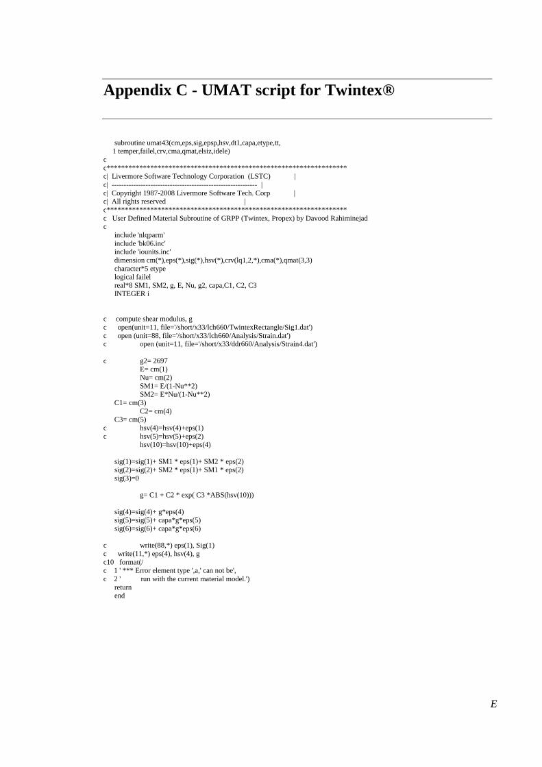
E
Appendix C - UMAT script for Twintex®
subroutine umat43(cm,eps,sig,epsp,hsv,dt1,capa,etype,tt, 1 temper,failel,crv,cma,qmat,elsiz,idele)
c
c****************************************************************** c| Livermore Software Technology Corporation (LSTC) |
c| ------------------------------------------------------------ |
c| Copyright 1987-2008 Livermore Software Tech. Corp | c| All rights reserved |
c******************************************************************
c User Defined Material Subroutine of GRPP (Twintex, Propex) by Davood Rahiminejad c
include 'nlqparm'
include 'bk06.inc' include 'iounits.inc'
dimension cm(*),eps(*),sig(*),hsv(*),crv(lq1,2,*),cma(*),qmat(3,3)
character*5 etype logical failel
real*8 SM1, SM2, g, E, Nu, g2, capa,C1, C2, C3 INTEGER i
c compute shear modulus, g
c open(unit=11, file='/short/x33/lch660/TwintexRectangle/Sig1.dat')
c open (unit=88, file='/short/x33/lch660/Analysis/Strain.dat') c open (unit=11, file='/short/x33/ddr660/Analysis/Strain4.dat')
c g2= 2697 E= cm(1)
Nu= cm(2)
SM1= E/(1-Nu**2) SM2= E*Nu/(1-Nu**2)
C1= cm(3)
C2= cm(4) C3= cm(5)
c hsv(4)=hsv(4)+eps(1)
c hsv(5)=hsv(5)+eps(2) hsv(10)=hsv(10)+eps(4)
sig(1)=sig(1)+ SM1 * eps(1)+ SM2 * eps(2) sig(2)=sig(2)+ SM2 * eps(1)+ SM1 * eps(2)
sig(3)=0
g= C1 + C2 * exp( C3 *ABS(hsv(10)))
sig(4)=sig(4)+ g*eps(4) sig(5)=sig(5)+ capa*g*eps(5)
sig(6)=sig(6)+ capa*g*eps(6)
c write(88,*) eps(1), Sig(1)
c write(11,*) eps(4), hsv(4), g
c10 format(/
c 1 ' *** Error element type ',a,' can not be',
c 2 ' run with the current material model.')
return end