atmosphere

Article

An Investigation of the Differences between theNorth American Dipole and NorthAtlantic Oscillation

Xuejing Zhou 1,3 , Wei Wang 1, Ruiqiang Ding 2,3,*, Jianping Li 2,4, Zhaolu Hou 3 and Wei Xie 1,3

1 College of Atmospheric Science, Chengdu University of Information Technology, and Plateau Atmosphericand Environment Laboratory of Sichuan Province, Chengdu 610225, China; zhouxuejing08@163.com (X.Z.);wei2009@cuit.edu.cn (W.W.); xiewei_11@126.com (W.X.)

2 Laboratory for Regional Oceanography and Numerical Modeling, Qingdao National Laboratory for MarineScience and Technology, Qingdao 266061, China; ljp@bnu.edu.cn

3 State Key Laboratory of Numerical Modeling for Atmospheric Sciences and Geophysical FluidDynamics (LASG), Institute of Atmospheric Physics, Chinese Academy of Sciences, Beijing 100029, China;hzl@lasg.iap.ac.cn

4 College of Global Change and Earth System Sciences (GCESS), Beijing Normal University,Beijing 100875, China

* Correspondence: drq@mail.iap.ac.cn

Received: 21 November 2018; Accepted: 15 January 2019; Published: 1 February 2019�����������������

Abstract: This study examines the differences between the North American dipole (NAD) and theNorth American Oscillation (NAO) in terms of their spatial structure, temporal variations, andclimate impacts. The results indicate that the sea level pressure anomalies associated with the NADare located in more western and southern areas than those associated with the NAO, and that theNAD has its own temporal variability. In addition, the NAD has a greater influence on sea surfacetemperature (SST) and precipitation anomalies in the northern tropical Atlantic (NTA) than the NAOdoes in the North Atlantic. In the tropical Pacific, the NAD tends to be more effective in forcing SSTwarming during spring in the northeastern subtropical Pacific (NESP). This can extend equatorwardto reach the equatorial central Pacific in the autumn, finally leading to a central Pacific (CP)-type ElNiño event. In contrast, the NAO induces only weak SST warming over the NESP, so that a CP-typeEl Niño event does not occur. Additional analysis indicates that the influence of the NAO can pass tothe tropical Pacific only when the NAD and NAO have the same sign, suggesting that the NAD mayserve as an important bridge linking the NAO to El Niño–Southern Oscillation (ENSO).

Keywords: North American dipole (NAD); North Atlantic Oscillation (NAO); central Pacific(CP)-type El Niño

1. Introduction

The North Atlantic Oscillation (NAO) is the dominant mode of atmospheric circulation variabilityover the North Atlantic sector, and it has long been recognized as a large-scale south–north seesawin atmosphere pressure, between the Azores High in the South and the Icelandic Low in the North.A positive (negative) NAO indicates that the intensity of both the Icelandic Low and the Azores Highare simultaneously enhanced (weakened) [1–6]. The NAO occurs throughout the year, but it is mostpronounced during the northern winter [7,8]. A number of previous studies have demonstrated that theNAO has a strong influence on regional weather and climate variation over the northern hemisphere.For instance, the NAO not only directly affects regional distributions of surface temperature andprecipitation over the North Atlantic and its adjacent land areas, including North America, North

Atmosphere 2019, 10, 58; doi:10.3390/atmos10020058 www.mdpi.com/journal/atmosphere

Atmosphere 2019, 10, 58 2 of 13

Africa, and Europe [5,9–13], but also affects East Asia via air–sea interactions [14–16]. Furthermore,many studies have also indicated that the associations of the NAO with Arctic sea ice variability andNorthern Hemisphere ozone are significant [17–21]. In addition, the NAO forces the tripole patternof sea surface temperature (SST) anomalies in the North Atlantic during winter via a change in theair–sea heat flux, as has been described in previous studies [21,22]. The tripole pattern is characterizedby a positive SST anomaly to the east of the United States along 35◦ N, and a negative SST anomaly tothe northeast and southeast respectively [13,23,24]. This tripole pattern is also the leading pattern ofSST variability during winter over the North Atlantic, and has been verified by many observationsand coupled ocean–atmosphere models [25,26].

A recent study by Ding et al. [27] reported that there is a south–north dipole pattern of sea levelpressure (SLP) anomalies over the western tropical North Atlantic and northeastern North America,which they called the North American dipole (NAD). The positive NAD pattern manifests as positiveSLP anomalies in the western tropical North Atlantic, and as negative SLP anomalies over northeasternNorth America. In contrast to the NAO, both the wintertime NAD and NAO have a dipole distributionof SLP anomalies over the North Atlantic, but the activity center of the NAD is more westward and closerto the North Pacific than that of the NAO. As a result, the NAD is more closely related to the centralPacific (CP)-type El Niño, whose maximum positive SST anomalies are located in the central equatorialPacific [28,29]. Ding et al. [27] demonstrated that the wintertime NAD can induce spring SST coolingin the northern tropical Atlantic (NTA; 85◦ W–20◦ E, 0–15◦ N), which in turn affects the developmentof the Pacific meridional mode (PMM) [30] through the subtropical teleconnection mechanism (STM)proposed by Ham et al. [31]. Through the wind-evaporation-SST (WES) feedback [32], the SST warmingassociated with the PMM over the northern subtropical Pacific extends southwestward and reachesthe central equatorial Pacific during summer, finally leading to a CP-type El Niño event. Therefore,the NAD may serve as a unique precursor signal for the CP-type El Niño.

Given that both the NAD and NAO influence the NTA SST, it would be interesting to investigatethe differences between their spatial characteristics, temporal variation, and climatic effects. In aprevious study, Ding et al. [27] presented a preliminary discussion of the differences between the NADand NAO, but these differences are still not fully understood. Therefore, the purpose of this study is toexplore the differences between them in greater depth. The remainder of this paper is organized asfollows: A description of our datasets and methodology is presented in Section 2; Section 3 comparesthe spatial features, temporal variations, and climatic impacts of the NAD and NAO; a summary anddiscussion are provided in Section 4.

2. Data and Methodology

The datasets used in this study were the monthly mean SLP, surface temperature, and surface windobtained from the National Centers for Environmental Prediction–National Center for AtmosphericResearch (NCEP−NCAR) reanalysis datasets, with a horizontal resolution of 2.5◦ × 2.5◦ [33].The precipitation dataset was taken from the NOAA Climate Prediction Center (CPC) Merged Analysisof Precipitation (CMAP), which produces a monthly analysis of global precipitation in which gaugeobservations are merged with precipitation estimates from several satellite-based algorithms (infraredand microwave) at a spatial resolution of 2.5◦ × 2.5◦ [34]. The monthly mean SST data were extractedfrom the National Oceanic and Atmospheric Administration (NOAA) Extended Reconstructed SST,version 3b (ERSSTv3b) dataset [35]. The ERSSTv3b dataset has a 2◦ × 2◦ horizontal resolution andruns from 1854 to the present.

The NAO index (NAOI) used in this paper is defined as the difference between 35◦ N and 65◦

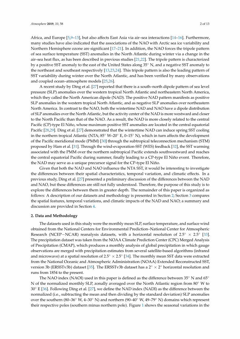
N of the normalized monthly SLP, zonally averaged over the North Atlantic region from 80◦ W to30◦ E [36]. Following Ding et al. [27], we define the NAD index (NADI) as the difference between thenormalized (i.e., subtracting the mean and then dividing by the standard deviation) SLP anomaliesover the southern (80–36◦ W, 4–30◦ N) and northern (90–40◦ W, 49–79◦ N) domains which representtheir respective poles (southern minus northern pole). Figure 1 shows the seasonal variations in the

Atmosphere 2019, 10, 58 3 of 13

standard deviations of the monthly NADI (a) and NAOI (b). Note that both the NAD and NAO exhibittight phase-locking characteristics. They both attain the maximum variance from December to March(DJFM), which is consistent with the results of previous studies [8,37]. Thus, we used the extendedwinter (DJFM) averaged NADI (NAOI) when the NAD (NAO) is most active, instead of the traditionalwinter (DJF) averaged NADI (NAOI). Our calculation also indicated that the difference of the resultsbetween the two NADI (NAOI) is very small (not shown).

We analyzed the period 1979−2016, because SST, surface wind, and precipitation were all availablefor this span. The statistical techniques used in this study were correlation, partial correlation,and composite analysis.

Atmosphere 2019, 10, x FOR PEER REVIEW 3 of 14

their respective poles (southern minus northern pole). Figure 1 shows the seasonal variations in the standard deviations of the monthly NADI (a) and NAOI (b). Note that both the NAD and NAO exhibit tight phase-locking characteristics. They both attain the maximum variance from December to March (DJFM), which is consistent with the results of previous studies [8,37]. Thus, we used the extended winter (DJFM) averaged NADI (NAOI) when the NAD (NAO) is most active, instead of the traditional winter (DJF) averaged NADI (NAOI). Our calculation also indicated that the difference of the results between the two NADI (NAOI) is very small (not shown).

We analyzed the period 1979−2016, because SST, surface wind, and precipitation were all available for this span. The statistical techniques used in this study were correlation, partial correlation, and composite analysis.

Figure 1. (a) Seasonal variations of the standard deviation of the NADI; (b) as (a), but for NAOI.

3. Results

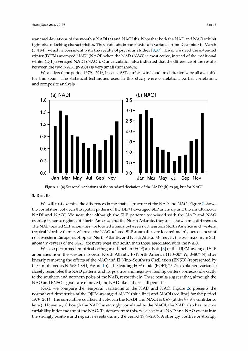
We will first examine the differences in the spatial structure of the NAD and NAO. Figure 2 shows the correlation between the spatial pattern of the DJFM-averaged SLP anomaly and the simultaneous NADI and NAOI. We note that although the SLP patterns associated with the NAD and NAO overlap in some regions of North America and the North Atlantic, they also show some differences. The NAD-related SLP anomalies are located mainly between northeastern North America and western tropical North Atlantic, whereas the NAO-related SLP anomalies are located mainly across most of northwestern Europe, subtropical North Atlantic, and North Africa. Moreover, the two maximum SLP anomaly centers of the NAD are more west and south than those associated with the NAO.

Figure 1. (a) Seasonal variations of the standard deviation of the NADI; (b) as (a), but for NAOI.

3. Results

We will first examine the differences in the spatial structure of the NAD and NAO. Figure 2 showsthe correlation between the spatial pattern of the DJFM-averaged SLP anomaly and the simultaneousNADI and NAOI. We note that although the SLP patterns associated with the NAD and NAOoverlap in some regions of North America and the North Atlantic, they also show some differences.The NAD-related SLP anomalies are located mainly between northeastern North America and westerntropical North Atlantic, whereas the NAO-related SLP anomalies are located mainly across most ofnorthwestern Europe, subtropical North Atlantic, and North Africa. Moreover, the two maximum SLPanomaly centers of the NAD are more west and south than those associated with the NAO.

We also performed empirical orthogonal function (EOF) analysis [3] of the DJFM-averaged SLPanomalies from the western tropical North Atlantic to North America (110–30◦ W, 0–80◦ N) afterlinearly removing the effects of the NAO and El Niño–Southern Oscillation (ENSO) (represented bythe simultaneous Niño3.4 SST; Figure 1b). The leading EOF mode (EOF1; 25.7% explained variance)closely resembles the NAD pattern, and its positive and negative loading centers correspond exactlyto the southern and northern poles of the NAD, respectively. These results suggest that, although theNAO and ENSO signals are removed, the NAD-like pattern still persists.

Next, we compare the temporal variations of the NAD and NAO. Figure 2c presents thenormalized time series of the DJFM-averaged NADI (blue line) and NAOI (red line) for the period1979–2016. The correlation coefficient between the NADI and NAOI is 0.67 (at the 99.9% confidencelevel). However, although the NADI is strongly correlated to the NAOI, the NAD also has its ownvariability independent of the NAO. To demonstrate this, we classify all NAD and NAO events intothe strongly positive and negative events during the period 1979–2016. A strongly positive or strongly

Atmosphere 2019, 10, 58 4 of 13

negative NAD (NAO) event is defined as a year when its index was greater than 1.0 with positivestandard deviation (>1.0) or less than 1.0 with negative standard deviation (<−1.0), while years thatfell outside these criteria were labelled ‘no NAO’ or ‘no NAD’ (Table 1). Only four positive NADevents (1988, 1989, 2006, and 2013) and three negative NAD events (2009, 2010, and 2012) occurredsimultaneously with strong NAO events. The remaining three positive (1985, 1990, and 2002) andfour negative (1980, 1982, 1997, and 2004) NAD events were not accompanied by strong NAO events.In particular, 2002 was a year in which the NADI was 1.2 (one of the strongly positive NAD events),while the NAOI was −0.6. In addition, 1982 was a typical year in which a strongly negative NADevent was accompanied by a strongly positive NAO event (the NADI and NAOI were −1.7 and 1.0,respectively). This result indicates that the fluctuations of the NAD are not completely consistent withthose of the NAO, and that the NAD has its own temporal variability that is independent of the NAO.Atmosphere 2019, 10, x FOR PEER REVIEW 4 of 14

Figure 2. (a) Maps of correlation between the DJFM-averaged SLP anomalies and the simultaneous NADI (blue lines) and NAOI (red lines). The contour interval is 0.1. Only correlations greater than 0.5 are shown; (b) spatial pattern of the first leading EOF mode from North America to the North Atlantic (110–30° W, 0–80° N); (c) time series of the DJFM-averaged NADI (blue line) and NAOI (red line). The horizontal dashed lines indicate ±1 standard deviation. The correlation coefficient (R) between the NADI and NAOI is shown in the lower left corner.

We also performed empirical orthogonal function (EOF) analysis [3] of the DJFM-averaged SLP anomalies from the western tropical North Atlantic to North America (110–30° W, 0–80° N) after linearly removing the effects of the NAO and El Niño–Southern Oscillation (ENSO) (represented by the simultaneous Niño3.4 SST; Figure 1b). The leading EOF mode (EOF1; 25.7% explained variance) closely resembles the NAD pattern, and its positive and negative loading centers correspond exactly to the southern and northern poles of the NAD, respectively. These results suggest that, although the NAO and ENSO signals are removed, the NAD-like pattern still persists.

Next, we compare the temporal variations of the NAD and NAO. Figure 2c presents the normalized time series of the DJFM-averaged NADI (blue line) and NAOI (red line) for the period 1979–2016. The correlation coefficient between the NADI and NAOI is 0.67 (at the 99.9% confidence level). However, although the NADI is strongly correlated to the NAOI, the NAD also has its own variability independent of the NAO. To demonstrate this, we classify all NAD and NAO events into the strongly positive and negative events during the period 1979–2016. A strongly positive or strongly negative NAD (NAO) event is defined as a year when its index was greater than 1.0 with positive standard deviation (>1.0) or less than 1.0 with negative standard deviation (<–1.0), while years that fell outside these criteria were labelled ‘no NAO’ or ‘no NAD’ (Table 1). Only four positive NAD events (1988, 1989, 2006, and 2013) and three negative NAD events (2009, 2010, and 2012) occurred simultaneously with strong NAO events. The remaining three positive (1985, 1990, and 2002) and four negative (1980, 1982, 1997, and 2004) NAD events were not accompanied by strong NAO events. In particular, 2002 was a year in which the NADI was 1.2 (one of the strongly

Figure 2. (a) Maps of correlation between the DJFM-averaged SLP anomalies and the simultaneousNADI (blue lines) and NAOI (red lines). The contour interval is 0.1. Only correlations greater than 0.5are shown; (b) spatial pattern of the first leading EOF mode from North America to the North Atlantic(110–30◦ W, 0–80◦ N); (c) time series of the DJFM-averaged NADI (blue line) and NAOI (red line). Thehorizontal dashed lines indicate ±1 standard deviation. The correlation coefficient (R) between theNADI and NAOI is shown in the lower left corner.

The above analyses show that there are differences in the spatial patterns and temporal variabilityof the NAD and NAO, and these differences may be the cause of their differing climatic impacts.Consequently, we next consider the seasonal evolution of climatic impacts. The maps showing thecorrelation of the three-month-averaged SST, surface wind, and precipitation anomalies with the NADIand NAOI for the December–February (DJF) concurrent with the two indices, and several lead times(March–May: MAM, June–August: JJA, and September–November: SON) are shown in Figure 3. Note thatalthough there are some similarities among the correlation maps, the differences are also obvious.

Atmosphere 2019, 10, 58 5 of 13

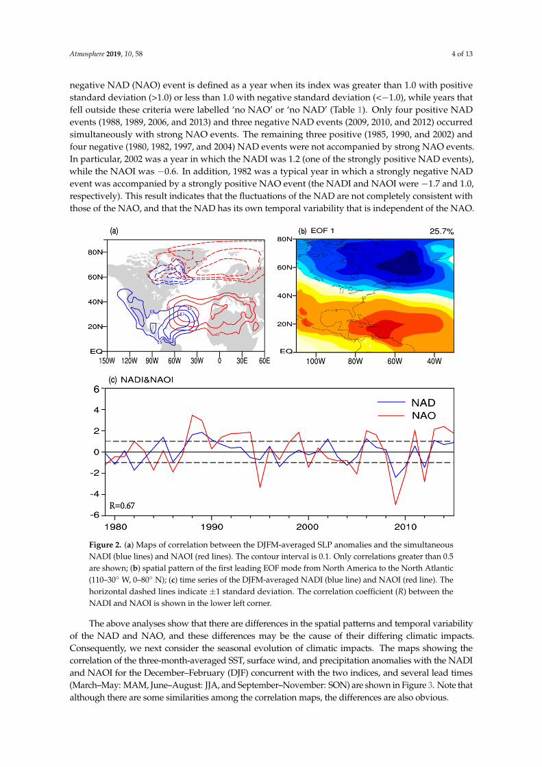
Table 1. Classification of years in which positive (negative) NAD events are or are not simultaneouswith a positive (negative) NAO event during the period 1979–2016 (see text for the definition of theNAD and NAO events).

Type Positive NAD No NAD Negative NAD

Positive NAO 1988, 1989, 2006, 2013 1991, 1992, 1993, 1994, 1999,2007, 2011, 2014, 2015 1982

Negative NAO – 1979, 1984, 1986, 1995, 2000, 2005 2009, 2010, 2012No NAO 1985, 1990, 2002 – 1980, 1997, 2004

Atmosphere 2019, 10, x FOR PEER REVIEW 6 of 14

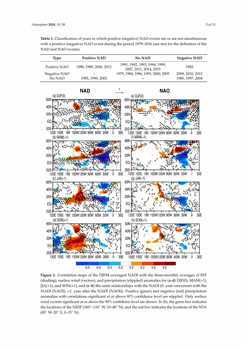
Figure 3. Correlation maps of the DJFM–averaged NADI with the three-monthly averages of SST (shading), surface wind (vectors), and precipitation (stippled) anomalies for (a–d) DJF(0), MAM(+1), JJA(+1), and SON(+1), and (e–h) the same relationships with the NAOI (0: year concurrent with the NADI (NAOI); +1: year after the NADI (NAOI)). Positive (green) and negative (red) precipitation anomalies with correlations significant at or above 90% confidence level are stippled. Only surface wind vectors significant at or above the 90% confidence level are shown. In (b), the green box indicates the locations of the NESP (160°–110° W, 10–40° N), and the red box indicates the locations of the NTA (85° W–20° E, 0–15° N).

In the North Atlantic, both the NAD and NAO can force a tripole-like SST anomaly pattern by changing the latent heat flux in winter (DJF; Figure 3a,e) and spring (MAM; Figure 3b,f). However, there are some differences between their related tripole-like SST anomaly patterns. For example, the NAD has more significant correlations in the western North Atlantic than does the NAO. In particular, the major difference is in the NTA region (indicated by the red box in Figure 3b), where the influence of the NAO on the NTA region is much weaker than that of the NAD. The correlation coefficient (R) between the NADI and the following MAM-averaged NTA SST is −0.64 (significant at the 99.9% confidence level), which is higher than that between the NAOI and the following MAM-averaged NTA SST (R = −0.39; significant at the 95% confidence level; see also Figure 4a). As Ding et al. [26] mentioned, because the southern pole of the NAD is located much farther west and south (i.e., towards the NTA region) than the NAO, the NAD-related surface wind anomalies

Figure 3. Correlation maps of the DJFM–averaged NADI with the three-monthly averages of SST(shading), surface wind (vectors), and precipitation (stippled) anomalies for (a–d) DJF(0), MAM(+1),JJA(+1), and SON(+1), and (e–h) the same relationships with the NAOI (0: year concurrent with theNADI (NAOI); +1: year after the NADI (NAOI)). Positive (green) and negative (red) precipitationanomalies with correlations significant at or above 90% confidence level are stippled. Only surfacewind vectors significant at or above the 90% confidence level are shown. In (b), the green box indicatesthe locations of the NESP (160◦–110◦ W, 10–40◦ N), and the red box indicates the locations of the NTA(85◦ W–20◦ E, 0–15◦ N).

Atmosphere 2019, 10, 58 6 of 13

In the North Atlantic, both the NAD and NAO can force a tripole-like SST anomaly pattern bychanging the latent heat flux in winter (DJF; Figure 3a,e) and spring (MAM; Figure 3b,f). However,there are some differences between their related tripole-like SST anomaly patterns. For example, theNAD has more significant correlations in the western North Atlantic than does the NAO. In particular,the major difference is in the NTA region (indicated by the red box in Figure 3b), where the influenceof the NAO on the NTA region is much weaker than that of the NAD. The correlation coefficient(R) between the NADI and the following MAM-averaged NTA SST is −0.64 (significant at the 99.9%confidence level), which is higher than that between the NAOI and the following MAM-averagedNTA SST (R = −0.39; significant at the 95% confidence level; see also Figure 4a). As Ding et al. [26]mentioned, because the southern pole of the NAD is located much farther west and south (i.e., towardsthe NTA region) than the NAO, the NAD-related surface wind anomalies extend farther to the westand southwest towards the NTA region than those related to the NAO. Therefore, in contrast to theNAO, the NAD has a closer relationship with the NTA SST anomalies.

Atmosphere 2019, 10, x FOR PEER REVIEW 7 of 14

extend farther to the west and southwest towards the NTA region than those related to the NAO. Therefore, in contrast to the NAO, the NAD has a closer relationship with the NTA SST anomalies.

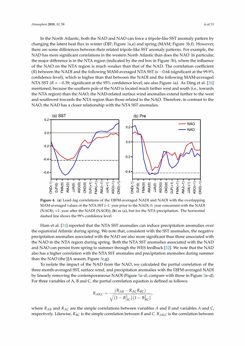
Figure 4. (a) Lead–lag correlations of the DJFM-averaged NADI and NAOI with the overlapping MAM-averaged values of the NTA SST (–1: year prior to the NADI; 0: year concurrent with the NADI (NAOI); +1: year after the NADI (NAOI)); (b) as (a), but for the NTA precipitation. The horizontal dashed line shows the 99% confidence level.

Ham et al. [31] reported that the NTA SST anomalies can induce precipitation anomalies over the equatorial Atlantic during spring. We note that, consistent with the SST anomalies, the negative precipitation anomalies associated with the NAD are also more significant than those associated with the NAO in the NTA region during spring. Both the NTA SST anomalies associated with the NAD and NAO can persist from spring to summer through the WES feedback [32]. We note that the NAD also has a higher correlation with the NTA SST anomalies and precipitation anomalies during summer than the NAO (the JJA season; Figure 3c,g).

To isolate the impact of the NAD from the NAO, we calculated the partial correlation of the three-month-averaged SST, surface wind, and precipitation anomalies with the DJFM-averaged NADI by linearly removing the contemporaneous NAOI (Figure 5a–d; compare with those in Figure 3a–d). For three variables of A, B and C, the partial correlation equation is defined as follows: 𝑅 , = (𝑅 − 𝑅 𝑅 )(1 − 𝑅 )(1 − 𝑅 ), where 𝑅 and 𝑅 are the simple correlations between variables A and B and variables A and C, respectively. Likewise, 𝑅 is the simple correlation between B and C. 𝑅 , is the correlation between two variables, A and B, after removing the effect of another variable, C. Variables A, B, and C in this place can be taken as NADI, SST (or surface wind, precipitation) anomalies, and NAOI.

With the removal of the NAO effect, the tripole-like SST anomaly pattern and precipitation anomalies associated with the NAD still exist in the North Atlantic during spring and summer. In contrast, with the NAD effect removed (Figure 5e–h), the tripole-like SST anomaly pattern associated with the NAO obviously weakens, especially in the NTA region, where significant SST and precipitation anomalies become indistinct. Therefore, the NAD tends to have a greater influence on climate variability in the NTA region than does the NAO.

Figure 4. (a) Lead–lag correlations of the DJFM-averaged NADI and NAOI with the overlappingMAM-averaged values of the NTA SST (–1: year prior to the NADI; 0: year concurrent with the NADI(NAOI); +1: year after the NADI (NAOI)); (b) as (a), but for the NTA precipitation. The horizontaldashed line shows the 99% confidence level.

Ham et al. [31] reported that the NTA SST anomalies can induce precipitation anomalies overthe equatorial Atlantic during spring. We note that, consistent with the SST anomalies, the negativeprecipitation anomalies associated with the NAD are also more significant than those associated withthe NAO in the NTA region during spring. Both the NTA SST anomalies associated with the NADand NAO can persist from spring to summer through the WES feedback [32]. We note that the NADalso has a higher correlation with the NTA SST anomalies and precipitation anomalies during summerthan the NAO (the JJA season; Figure 3c,g).

To isolate the impact of the NAD from the NAO, we calculated the partial correlation of thethree-month-averaged SST, surface wind, and precipitation anomalies with the DJFM-averaged NADIby linearly removing the contemporaneous NAOI (Figure 5a–d; compare with those in Figure 3a–d).For three variables of A, B and C, the partial correlation equation is defined as follows:

RAB,C =(RAB − RACRBC)√(1 − R2

AC)(

1 − R2BC) ,

where RAB and RAC are the simple correlations between variables A and B and variables A and C,respectively. Likewise, RBC is the simple correlation between B and C. RAB,C is the correlation between

Atmosphere 2019, 10, 58 7 of 13

two variables, A and B, after removing the effect of another variable, C. Variables A, B, and C in thisplace can be taken as NADI, SST (or surface wind, precipitation) anomalies, and NAOI.

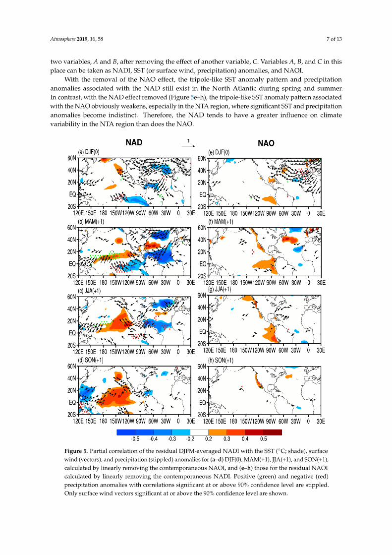
With the removal of the NAO effect, the tripole-like SST anomaly pattern and precipitationanomalies associated with the NAD still exist in the North Atlantic during spring and summer.In contrast, with the NAD effect removed (Figure 5e–h), the tripole-like SST anomaly pattern associatedwith the NAO obviously weakens, especially in the NTA region, where significant SST and precipitationanomalies become indistinct. Therefore, the NAD tends to have a greater influence on climatevariability in the NTA region than does the NAO.

Atmosphere 2019, 10, x FOR PEER REVIEW 8 of 14

Figure 5. Partial correlation of the residual DJFM-averaged NADI with the SST (°C; shade), surface wind (vectors), and precipitation (stippled) anomalies for (a–d) DJF(0), MAM(+1), JJA(+1), and SON(+1), calculated by linearly removing the contemporaneous NAOI, and (e–h) those for the residual NAOI calculated by linearly removing the contemporaneous NADI. Positive (green) and negative (red) precipitation anomalies with correlations significant at or above 90% confidence level are stippled. Only surface wind vectors significant at or above the 90% confidence level are shown.

In addition to the differences in the North Atlantic presented above, there are also some differences in the climatic effects of the NAD and NAO in the tropical Pacific. During spring (Figure 3b), significant positive SST anomalies associated with the NAD develop in the northeastern subtropical Pacific (NESP; 160–110° W, 10–40° N; indicated by the green box in Figure 3b) region. The NESP SST warming associated with the NAD extends equatorward during summer (Figure 3c), and is associated with significant positive precipitation anomalies in the central-eastern equatorial Pacific. During autumn (SON; Figure 3d,h), the SST warming associated with the NAD reaches the equatorial central Pacific, and a marked CP-type El Niño pattern is established. In contrast, weak SST anomalies (not significant at the 90% confidence level) associated with the NAO occur in the NESP region during spring. These weak SST anomalies associated with the NAO do not show

Figure 5. Partial correlation of the residual DJFM-averaged NADI with the SST (◦C; shade), surfacewind (vectors), and precipitation (stippled) anomalies for (a–d) DJF(0), MAM(+1), JJA(+1), and SON(+1),calculated by linearly removing the contemporaneous NAOI, and (e–h) those for the residual NAOIcalculated by linearly removing the contemporaneous NADI. Positive (green) and negative (red)precipitation anomalies with correlations significant at or above 90% confidence level are stippled.Only surface wind vectors significant at or above the 90% confidence level are shown.

Atmosphere 2019, 10, 58 8 of 13

In addition to the differences in the North Atlantic presented above, there are also some differencesin the climatic effects of the NAD and NAO in the tropical Pacific. During spring (Figure 3b), significantpositive SST anomalies associated with the NAD develop in the northeastern subtropical Pacific (NESP;160–110◦ W, 10–40◦ N; indicated by the green box in Figure 3b) region. The NESP SST warmingassociated with the NAD extends equatorward during summer (Figure 3c), and is associated withsignificant positive precipitation anomalies in the central-eastern equatorial Pacific. During autumn(SON; Figure 3d,h), the SST warming associated with the NAD reaches the equatorial central Pacific,and a marked CP-type El Niño pattern is established. In contrast, weak SST anomalies (not significantat the 90% confidence level) associated with the NAO occur in the NESP region during spring. Theseweak SST anomalies associated with the NAO do not show obvious equatorward propagation duringsummer (Figure 3c,g). As a result, the CP-type El Niño pattern associated with the NAO is indistinctduring the following winter. Therefore, we conclude that in contrast to the NAO, the NAD may alsoexert a stronger effect on the tropical Pacific.

There are two possible reasons why the NAD can significantly impact the tropical Pacific.Compared with the NAO, the southern pole of the NAD is much closer to the tropical Pacific. Thus,the NAD has a stronger effect on the NESP SST warming during spring via its associated concurrentanticyclonic flow. On the other hand, the above results have shown that the NAD influences theNTA SST more than the NAO. According to Ham et al. [31], the NTA SST cooling during spring caninduce an anticyclonic flow over the NESP region as a Gill-type Rossby wave [38] response. Therefore,the NAD can exert a stronger effect on the NESP SST warming by influencing the NTA SST. Finally,in contrast to the NAO, the NAD may play a more important role in influencing the occurrence ofCP-type El Niño, owing to its effectiveness at forcing the NESP SST warming.

With the removal of the NAO effect, there are some reductions in the correlations of SST, surfacewind, and precipitation anomalies with the residual NADI in the tropical Pacific (Figure 5a–d),but the NESP SST warming associated with the NAD is still significant during spring (Figure 5c).The CP-type El Niño pattern associated with the NAD can also be seen in the tropical Pacific duringthe following autumn. In contrast, after removing the effect of the NAD (Figure 5e–h), significant SSTand precipitation anomalies associated with the NAO almost disappear in the tropical North Pacific.These results support the idea that the NAD has an important effect on climate change in the NorthAtlantic as well as the tropical Pacific.

To further examine the differences between the NAD and NAO, we classified the NAD and NAOevents into the following three groups: 1) positive (negative) NAD events that are not accompaniedby a positive (negative) NAO event (hereafter positive NAD only or negative NAD only); 2) positive(negative) NAO events that are not accompanied by a positive (negative) NAD event (hereafter positiveNAO only or negative NAO only); and 3) positive (negative) NAD events that are accompanied by apositive (negative) NAO event (hereafter positive NAD–NAO or negative NAD–NAO; as also listed inTable 1).

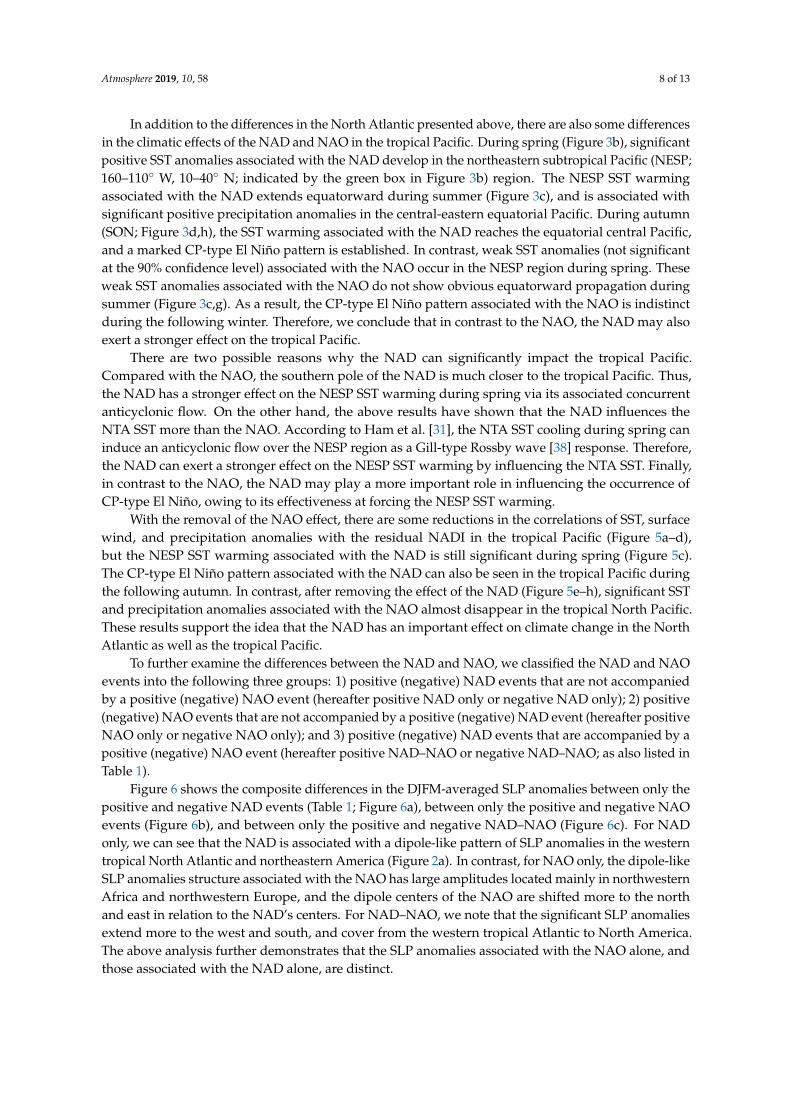
Figure 6 shows the composite differences in the DJFM-averaged SLP anomalies between only thepositive and negative NAD events (Table 1; Figure 6a), between only the positive and negative NAOevents (Figure 6b), and between only the positive and negative NAD–NAO (Figure 6c). For NADonly, we can see that the NAD is associated with a dipole-like pattern of SLP anomalies in the westerntropical North Atlantic and northeastern America (Figure 2a). In contrast, for NAO only, the dipole-likeSLP anomalies structure associated with the NAO has large amplitudes located mainly in northwesternAfrica and northwestern Europe, and the dipole centers of the NAO are shifted more to the northand east in relation to the NAD’s centers. For NAD–NAO, we note that the significant SLP anomaliesextend more to the west and south, and cover from the western tropical Atlantic to North America.The above analysis further demonstrates that the SLP anomalies associated with the NAO alone, andthose associated with the NAD alone, are distinct.

Atmosphere 2019, 10, 58 9 of 13

Atmosphere 2019, 10, x FOR PEER REVIEW 10 of 14

Figure 6. Composite differences of the DJFM-averaged SLP anomalies between (a) positive and negative NAD only, between (b) positive and negative NAO only, and between (c) positive and negative NAD–NAO. Anomalies significant at the 90% confidence level are stippled.

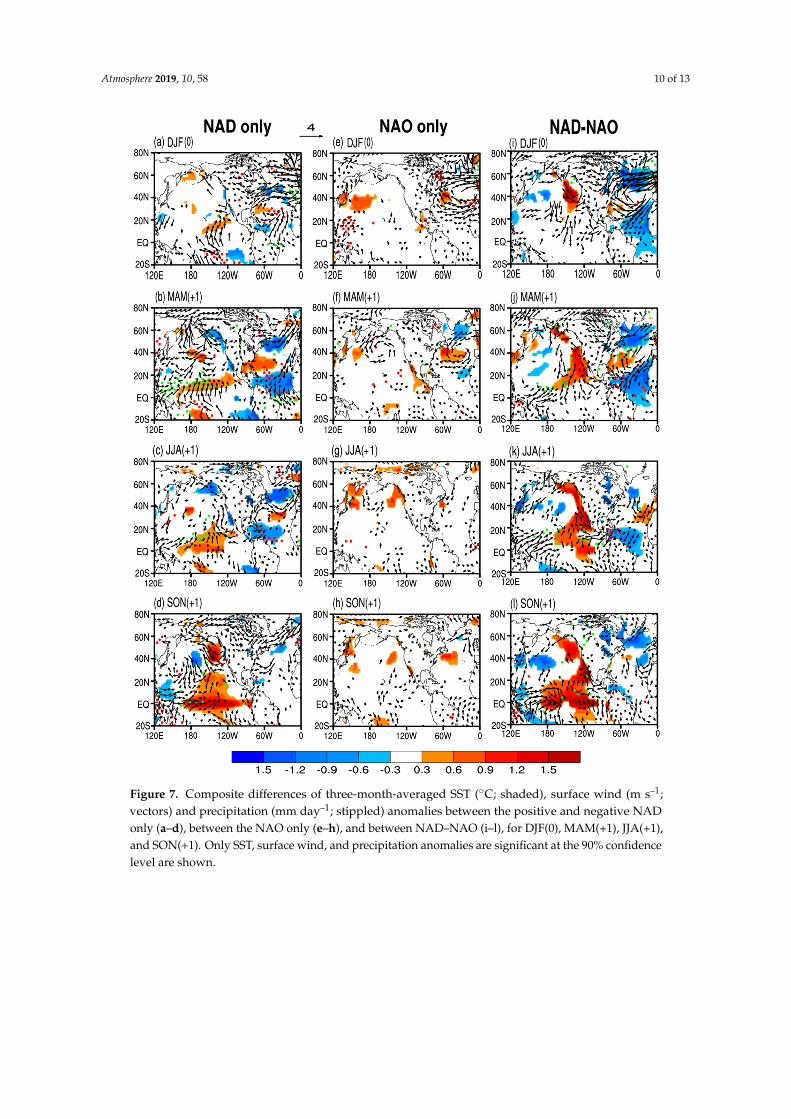
We next examined their climatic impacts by using the composite differences of the three-month-averaged SST, surface wind, and precipitation anomalies for the three groups for DJF, MAM, JJA, and SON (Figure 7). For NAD only, the tripole-like SST pattern during spring in the North Atlantic, and the CP-type El Niño pattern during autumn in the tropical Pacific, remain evident. However, for NAO only, the SST and precipitation anomalies in the North Atlantic and North Pacific are significantly weaker than those for NAD only. These results are consistent with the above analysis (Figure 3a), which suggests that the NAD may exert a stronger climatic effect on the NTA region and the tropical Pacific than the NAO. In addition, we note that the SST, surface wind, and precipitation anomalies in NAD–NAO are closely comparable to the NAD-only scenario, and the large difference between the two groups lies mainly in the tropical Pacific. Unlike the NAD-only class, the NAD–NAO group has stronger SST and precipitation anomalies in the tropical Pacific. These results indicate that the NAO alone has a very weak impact on the tropical Pacific, and the influence on the tropical Pacific will be strengthened when it coincides with the NAD.

Figure 6. Composite differences of the DJFM-averaged SLP anomalies between (a) positive andnegative NAD only, between (b) positive and negative NAO only, and between (c) positive andnegative NAD–NAO. Anomalies significant at the 90% confidence level are stippled.

We next examined their climatic impacts by using the composite differences of thethree-month-averaged SST, surface wind, and precipitation anomalies for the three groups for DJF,MAM, JJA, and SON (Figure 7). For NAD only, the tripole-like SST pattern during spring in theNorth Atlantic, and the CP-type El Niño pattern during autumn in the tropical Pacific, remain evident.However, for NAO only, the SST and precipitation anomalies in the North Atlantic and North Pacificare significantly weaker than those for NAD only. These results are consistent with the above analysis(Figure 3a), which suggests that the NAD may exert a stronger climatic effect on the NTA region andthe tropical Pacific than the NAO. In addition, we note that the SST, surface wind, and precipitationanomalies in NAD–NAO are closely comparable to the NAD-only scenario, and the large differencebetween the two groups lies mainly in the tropical Pacific. Unlike the NAD-only class, the NAD–NAOgroup has stronger SST and precipitation anomalies in the tropical Pacific. These results indicate thatthe NAO alone has a very weak impact on the tropical Pacific, and the influence on the tropical Pacificwill be strengthened when it coincides with the NAD.

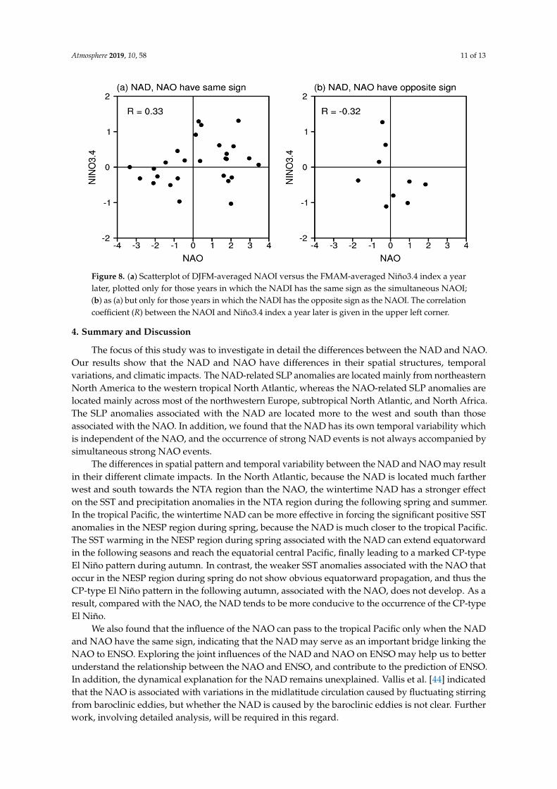
Previous studies indicated that the ENSO had no significant relationship with the NAO; thecorrelation between them is very low [39,40]. Although some studies found that there are moreoccurrences of negative NAD in the late winter during El Niño events, and of positive NAO in LaNiña events, there are still many uncertainties about the relationship between them [41–43]. However,we investigated the joint relationship between the NAD, the NAO, and ENSO through a scatterplotbetween the DJFM-averaged NADI and simultaneous NAOI, for the cases where they have the same(Figure 8a) or opposite (Figure 8b) sign. We note that the correlation between the NAO and Niño3.4indices is 0.33 (significant at the 90% confidence level for the 28 events) when the NADI and the NAOIhave the same sign (Figure 8a), whereas the correlation is −0.32 (not significant at the 90% confidencelevel for the 9 events) when the NADI and the NAOI have the opposite sign (Figure 8b). Therefore, theNAD may serve as a bridge linking the NAO to ENSO, suggesting that we should consider the role ofthe NAD while examining the NAO’s effect on the following ENSO events.

Atmosphere 2019, 10, 58 10 of 13

Atmosphere 2019, 10, x FOR PEER REVIEW 11 of 14

Figure 7. Composite differences of three-month-averaged SST (°C; shaded), surface wind (m s–1; vectors) and precipitation (mm day–1; stippled) anomalies between the positive and negative NAD only (a–d), between the NAO only (e–h), and between NAD–NAO (i–l), for DJF(0), MAM(+1), JJA(+1), and SON(+1). Only SST, surface wind, and precipitation anomalies are significant at the 90% confidence level are shown.

Previous studies indicated that the ENSO had no significant relationship with the NAO; the correlation between them is very low [39,40]. Although some studies found that there are more occurrences of negative NAD in the late winter during El Niño events, and of positive NAO in La Niña events, there are still many uncertainties about the relationship between them [41–43]. However, we investigated the joint relationship between the NAD, the NAO, and ENSO through a scatterplot between the DJFM-averaged NADI and simultaneous NAOI, for the cases where they have the same (Figure 8a) or opposite (Figure 8b) sign. We note that the correlation between the NAO and Niño3.4 indices is 0.33 (significant at the 90% confidence level for the 28 events) when the NADI and the NAOI have the same sign (Figure 8a), whereas the correlation is −0.32 (not significant at the 90% confidence level for the 9 events) when the NADI and the NAOI have the

Figure 7. Composite differences of three-month-averaged SST (◦C; shaded), surface wind (m s–1;vectors) and precipitation (mm day–1; stippled) anomalies between the positive and negative NADonly (a–d), between the NAO only (e–h), and between NAD–NAO (i–l), for DJF(0), MAM(+1), JJA(+1),and SON(+1). Only SST, surface wind, and precipitation anomalies are significant at the 90% confidencelevel are shown.

Atmosphere 2019, 10, 58 11 of 13

Atmosphere 2019, 10, x FOR PEER REVIEW 12 of 14

opposite sign (Figure 8b). Therefore, the NAD may serve as a bridge linking the NAO to ENSO, suggesting that we should consider the role of the NAD while examining the NAO’s effect on the following ENSO events.

Figure 8. (a) Scatterplot of DJFM-averaged NAOI versus the FMAM-averaged Niño3.4 index a year later, plotted only for those years in which the NADI has the same sign as the simultaneous NAOI; (b) as (a) but only for those years in which the NADI has the opposite sign as the NAOI. The correlation coefficient (R) between the NAOI and Niño3.4 index a year later is given in the upper left corner.

4. Summary and Discussion

The focus of this study was to investigate in detail the differences between the NAD and NAO. Our results show that the NAD and NAO have differences in their spatial structures, temporal variations, and climatic impacts. The NAD-related SLP anomalies are located mainly from northeastern North America to the western tropical North Atlantic, whereas the NAO-related SLP anomalies are located mainly across most of the northwestern Europe, subtropical North Atlantic, and North Africa. The SLP anomalies associated with the NAD are located more to the west and south than those associated with the NAO. In addition, we found that the NAD has its own temporal variability which is independent of the NAO, and the occurrence of strong NAD events is not always accompanied by simultaneous strong NAO events.

The differences in spatial pattern and temporal variability between the NAD and NAO may result in their different climate impacts. In the North Atlantic, because the NAD is located much farther west and south towards the NTA region than the NAO, the wintertime NAD has a stronger effect on the SST and precipitation anomalies in the NTA region during the following spring and summer. In the tropical Pacific, the wintertime NAD can be more effective in forcing the significant positive SST anomalies in the NESP region during spring, because the NAD is much closer to the tropical Pacific. The SST warming in the NESP region during spring associated with the NAD can extend equatorward in the following seasons and reach the equatorial central Pacific, finally leading to a marked CP-type El Niño pattern during autumn. In contrast, the weaker SST anomalies associated with the NAO that occur in the NESP region during spring do not show obvious equatorward propagation, and thus the CP-type El Niño pattern in the following autumn, associated with the NAO, does not develop. As a result, compared with the NAO, the NAD tends to be more conducive to the occurrence of the CP-type El Niño.

We also found that the influence of the NAO can pass to the tropical Pacific only when the NAD and NAO have the same sign, indicating that the NAD may serve as an important bridge linking the NAO to ENSO. Exploring the joint influences of the NAD and NAO on ENSO may help us to better understand the relationship between the NAO and ENSO, and contribute to the prediction of ENSO. In addition, the dynamical explanation for the NAD remains unexplained.

Figure 8. (a) Scatterplot of DJFM-averaged NAOI versus the FMAM-averaged Niño3.4 index a yearlater, plotted only for those years in which the NADI has the same sign as the simultaneous NAOI;(b) as (a) but only for those years in which the NADI has the opposite sign as the NAOI. The correlationcoefficient (R) between the NAOI and Niño3.4 index a year later is given in the upper left corner.

4. Summary and Discussion

The focus of this study was to investigate in detail the differences between the NAD and NAO.Our results show that the NAD and NAO have differences in their spatial structures, temporalvariations, and climatic impacts. The NAD-related SLP anomalies are located mainly from northeasternNorth America to the western tropical North Atlantic, whereas the NAO-related SLP anomalies arelocated mainly across most of the northwestern Europe, subtropical North Atlantic, and North Africa.The SLP anomalies associated with the NAD are located more to the west and south than thoseassociated with the NAO. In addition, we found that the NAD has its own temporal variability whichis independent of the NAO, and the occurrence of strong NAD events is not always accompanied bysimultaneous strong NAO events.

The differences in spatial pattern and temporal variability between the NAD and NAO may resultin their different climate impacts. In the North Atlantic, because the NAD is located much fartherwest and south towards the NTA region than the NAO, the wintertime NAD has a stronger effecton the SST and precipitation anomalies in the NTA region during the following spring and summer.In the tropical Pacific, the wintertime NAD can be more effective in forcing the significant positive SSTanomalies in the NESP region during spring, because the NAD is much closer to the tropical Pacific.The SST warming in the NESP region during spring associated with the NAD can extend equatorwardin the following seasons and reach the equatorial central Pacific, finally leading to a marked CP-typeEl Niño pattern during autumn. In contrast, the weaker SST anomalies associated with the NAO thatoccur in the NESP region during spring do not show obvious equatorward propagation, and thus theCP-type El Niño pattern in the following autumn, associated with the NAO, does not develop. As aresult, compared with the NAO, the NAD tends to be more conducive to the occurrence of the CP-typeEl Niño.

We also found that the influence of the NAO can pass to the tropical Pacific only when the NADand NAO have the same sign, indicating that the NAD may serve as an important bridge linking theNAO to ENSO. Exploring the joint influences of the NAD and NAO on ENSO may help us to betterunderstand the relationship between the NAO and ENSO, and contribute to the prediction of ENSO.In addition, the dynamical explanation for the NAD remains unexplained. Vallis et al. [44] indicatedthat the NAO is associated with variations in the midlatitude circulation caused by fluctuating stirringfrom baroclinic eddies, but whether the NAD is caused by the baroclinic eddies is not clear. Furtherwork, involving detailed analysis, will be required in this regard.

Atmosphere 2019, 10, 58 12 of 13

Author Contributions: Conceptualization, R.D. and J.L.; Methodology, R.D., X.Z. and Z.H.; Writing–originaldraft, X.Z. and R.D.; Writing–review and editing, X.Z. and R.D.; Validation, W.W.; Supervision, R.D., W.W., andW.X. All authors contributed to the discussion of the results and have read and approved the final manuscript.

Funding: This research was jointly supported by the 973 project of China (2016YFA0601801), the National Programon Global Change and Air–Sea Interaction (GASI-IPOVAI-06, GASI-IPOVAI-03), and the National Key TechnologyResearch and Development Program of the Ministry of Science and Technology of China (2015BAC03B07).

Conflicts of Interest: The authors declare no conflict of interest.

References

1. Walker, G.; Bliss, E. World weather V. Mem. R. Meteor. Soc. 1932, 4, 53–84.2. Van Loon, H.; Rogers, J. The Seesaw in Winter Temperatures between Greenland and Northern Europe. Part

I: General Description. Mon. Weather Rev. 1978, 106, 296–310. [CrossRef]3. Wallace, J.; Gutzler, D. Teleconnections in the Geopotential Height Field during the Northern Hemisphere

Winter. Mon. Weather Rev. 1981, 109, 784–812. [CrossRef]4. Rogers, J. The association between the North Atlantic Oscillation and the Southern Oscillation in the Northern

Hemisphere. Mon. Weather Rev. 1984, 112, 1999–2015. [CrossRef]5. Hurrell, J. Decadal trends in the North Atlantic Oscillation: Regional temperatures and precipitation. Science

1995, 269, 676–679. [CrossRef] [PubMed]6. Kjellström, E. North Atlantic Oscillation (NAO). In Encyclopedia of Marine Geosciences; Springer:

Berlin/Heidelberg, Germany, 2013; pp. 1–2.7. Barnston, A.; Livezey, R. Classification, Seasonality and Persistence of Low-Frequency Atmospheric

Circulation Patterns. Mon. Weather Rev. 1987, 115, 1083–1126. [CrossRef]8. Rogers, J. Patterns of Low-Frequency Monthly Sea Level Pressure Variability (1899–1986) and Associated

Wave Cyclone Frequencies. J. Clim. 1990, 3, 1364–1379. [CrossRef]9. Lamb, P.; Peppler, R. North Atlantic Oscillation: Concept and an application. Bull. Am. Meteorol. Soc. 1987,

68, 1218–1225. [CrossRef]10. Hurrell, J.; Van, L. Decadal variations associated with the North Atlantic Oscillation. J. Clim. 1997, 36,

301–326. [CrossRef]11. Kushnir, Y. Climatology: Europe’s winter prospects. Nature 1999, 398, 289–291. [CrossRef]12. Greatbatch, R. The North Atlantic Oscillation. Stoch. Environ. Res. Risk Assess. 2000, 14, 213–242. [CrossRef]13. Marshall, J.; Kushnir, Y.; Battisti, D. North Atlantic climate variability: Phenomena, impacts and mechanisms.

J. Clim. 2001, 21, 1863–1898. [CrossRef]14. Wu, B.; Wang, J. Possible impacts of winter Arctic Oscillation on Siberian high, the East Asian winter

monsoon and sea-ice extent. Adv. Atmos. Sci. 2002, 19, 297–320.15. Sung, M.; Kwon, W.; Baek, H.; Boo, K.; Lim, G.; Kug, J. A possible impact of the North Atlantic Oscillation

on the East Asian summer monsoon precipitation. Geophys. Res. Lett. 2006, 33, 493–495. [CrossRef]16. Shao, T.; Zhang, Y. Influence of Winter North Atlantic Oscillation on Spring Precipitation in China.

Plateau Meteorol. 2012, 31, 1225–1233. (In Chinese)17. Kwok, R.; Rothrock, D. Variability of Fram Strait ice flux and North Atlantic Oscillation. J. Geophys. Res.

1999, 104, 5177–5189. [CrossRef]18. Deser, C. On the teleconnectivity of the “Arctic Oscillation”. Geophys. Res. Lett. 2000, 27, 779–782. [CrossRef]19. Appenzeller, C.; Weiss, A.; Staehelin, J. North Atlantic Oscillation modulates total ozone winter trends.

Geophys. Res. Lett. 2000, 27, 1131–1134. [CrossRef]20. Thompson, D. Annular modes in the extratropical circulation. Part II: Trends. J. Clim. 2000, 13, 1018–1036.

[CrossRef]21. Cayan, D. Latent and sensible heat flux anomalies over the Northern Oceans: The connection to monthly

atmospheric circulation. J. Clim. 1992, 5, 354–370. [CrossRef]22. Cayan, D. Latent and Sensible Heat Flux Anomalies over the Northern Oceans: Driving the Sea Surface

Temperature. J. Phys. Oceanogr. 1992, 22, 859–881. [CrossRef]23. Czaja, A.; Frankignoul, C. Observed impact of Atlantic SST anomalies on the North Atlantic Oscillation.

J. Clim. 2002, 15, 606–623. [CrossRef]

Atmosphere 2019, 10, 58 13 of 13

24. Visbeck, M.; Chassignet, E.; Curry, R.; Delworth, T.; Dickson, R.; Krahmann, G. The ocean’s response toNorth Atlantic Oscillation variability. In North Atlantic Oscillation Climatic Significance & Environmental Impact;Hurrell, J., Kushnir, Y., Ottersen, G., Visbeck, M., Eds.; AGU Geophysical Monograph: Washington, DC,USA, 2003; Volume 134, pp. 113–146.

25. Halliwell, G. Simulation of North Atlantic decadal/multidecadal winter SST anomalies driven by basin-scaleatmospheric circulation anomalies. J. Phys. Oceanogr. 1998, 28, 5–21. [CrossRef]

26. Zhou, T.; Zhang, X.; Yu, Y. The North Atlantic Oscillation simulated by versions 2 and 4 of IAP/LASGGOALS Model. Adv. Atmos. Sci. 2000, 17, 601–616.

27. Ding, R.; Li, J.; Tseng, Y.; Yuan, C. Linking a sea level pressure anomaly dipole over North America to thecentral Pacific El Nino. Clim. Dyn. 2017, 49, 1321–1339. [CrossRef]

28. Yu, J.; Kao, H. Decadal changes of ENSO persistence barrier in SST and ocean heat content indices: 1958–2001.J. Geophys. Res. 2007, 112, 125–138. [CrossRef]

29. Kao, H.; Yu, J. Contrasting eastern-Pacific and central-Pacific types of ENSO. J. Clim. 2009, 22, 615–632.[CrossRef]

30. Chiang, J.; Vimont, D. Analogous Pacific and Atlantic meridional modes of tropical atmosphere–oceanvariability. J. Clim. 2004, 17, 4143–4158. [CrossRef]

31. Ham, Y.; Kug, J.; Park, J.; Jin, F. Sea surface temperature in the north tropical Atlantic as a trigger for ElNiño/Southern Oscillation events. Nat. Geosci. 2013, 6, 112–116. [CrossRef]

32. Xie, S.; Philander, S. A coupled ocean–atmosphere model of relevance to the ITCZ in the eastern Pacific.Tellus A 1994, 46, 340–350. [CrossRef]

33. Kalnay, E.; Kanamitsu, M.; Kistler, R. The NCEP/NCAR 40-Year Reanalysis Project. Bull. Am. Meteorol. Soc.1996, 77, 437–472. [CrossRef]

34. Xie, P.; Arkin, P. Global precipitation: A 17-year monthly analysis based on gauge observations, satelliteestimates, and numerical model outputs. Bull. Am. Meteorol. Soc. 1997, 78, 2539–2558. [CrossRef]

35. Smith, T.; Reynolds, R.; Peterson, T.; Lawrimore, J. Improvements to NOAA’s historical merged land–oceansurface temperature analysis (1880–2006). J. Clim. 2008, 21, 2283–2296. [CrossRef]

36. Li, J.; Wang, J. A new North Atlantic Oscillation index and its variability. Adv. Atmos. Sci. 2003, 20, 661–676.37. Portis, D.; Walsh, J.; Hamly, M.; Lamb, P. Seasonality of the North Atlantic Oscillation. J. Clim. 2001, 14,

2069–2078. [CrossRef]38. Gill, A. Some simple solutions for heat-induced tropical circulation. Q. J. Meteorol. Soc. 1980, 106, 447–462.

[CrossRef]39. Quadrelli, R.; Pavan, V.; Molteni, F. Wintertime variability of Mediterranean precipitation and its links with

large-scale circulation anomalies. Clim. Dyn. 2001, 17, 457–466. [CrossRef]40. Wang, C. Atlantic Climate Variability and Its Associated Atmospheric Circulation Cells. J. Clim. 1991, 15,

1516–1536. [CrossRef]41. Li, Y.; Lau, N. Impact of ENSO on the Atmospheric Variability over the North Atlantic in Late Winter-Role of

Transient Eddies. J. Clim. 2012, 25, 320–342. [CrossRef]42. Gouirand, I.; Moron, V. Variability of the impact of El Niño–southern oscillation on sea–level pressure

anomalies over the North Atlantic in January to March (1874–1996). Int. J. Clim. 2003, 23, 1549–1566.[CrossRef]

43. Pozo-Vázquez, D.; Gámiz-Fortis, S.; Tovar-Pescador, J. North Atlantic Winter SLP Anomalies Based on theAutumn ENSO State. J. Clim. 2005, 18, 97–103. [CrossRef]

44. Vallis, G.; Gerber, E.; Kushner, P.; Cash, B. A Mechanism and Simple Dynamical Model of the North AtlanticOscillation and Annular Modes. J. Atmos. 2004, 61, 264–280. [CrossRef]

© 2019 by the authors. Licensee MDPI, Basel, Switzerland. This article is an open accessarticle distributed under the terms and conditions of the Creative Commons Attribution(CC BY) license (http://creativecommons.org/licenses/by/4.0/).