Embed Size (px)
Citation preview
Clemson UniversityTigerPrints
All Dissertations Dissertations
12-2011
An Investigation of the Application of PhaseChange Materials in Practical ThermalManagement SystemsDavid EwingClemson University, [email protected]
Follow this and additional works at: https://tigerprints.clemson.edu/all_dissertations
Part of the Mechanical Engineering Commons
This Dissertation is brought to you for free and open access by the Dissertations at TigerPrints. It has been accepted for inclusion in All Dissertations byan authorized administrator of TigerPrints. For more information, please contact [email protected].
Recommended CitationEwing, David, "An Investigation of the Application of Phase Change Materials in Practical Thermal Management Systems" (2011). AllDissertations. 820.https://tigerprints.clemson.edu/all_dissertations/820

An Investigation of the Application of Phase Change Materials in Practical Thermal Management Systems
A Dissertation Presented to
the Graduate School of Clemson University
In Partial Fulfillment
of the Requirements for the Degree Doctor of Philosophy
Mechanical Engineering
by
David Ewing December 2011
Committee Members: Lin Ma, Committee Chair
Donald Beasley Richard Miller Chenning Tong

ii
Abstract
This work investigates the application of alternative cooling techniques to
thermal management. In the first section, this work presents models and extensive
simulation studies on an alternative cooling strategy based upon phase change materials
(PCMs) for the thermal management system of a LED headlight assembly. These studies
have shown that properly chosen PCMs, when suspended in metal foam matrices,
increased the thermal conductivity of the PCM. The increased thermal conductivity can
enhance the cooling characteristics of a practical thermal management system for a LED
headlight system. To further enhance the advantages of using PCMs, nanoparticle
enhanced fluids (nanofluids) are desirable as an additional source of cooling. The use of
nanofluids motivates the development of a new diagnostic tool for multiphase flows and
a minimization algorithm for analyzing the data. For this purpose, the second section of
this work develops a new technique that is based on wavelength-multiplexed laser
extinction (WMLE) to measure particle sizes in multiphase flows. In the final section of
this work, the simulated algorithm (SA) is investigated for analyzing the data collected in
this work. Specifically, the parallelization of the SA technique is investigated to reduce
the high computational cost associated with the SA algorithm.

iii
Acknowledgements
I owe my deepest gratitude to my supervisor, Dr. Lin Ma, for without his advice
and leadership this work would not be possible. His encouragement, guidance and
support are greatly appreciated. I would also like to thank Drs. Richard Miller, Donald
Beasley and Chenning Tong for serving on my advisory committee.
In addition, I would thank all of my colleagues in Dr. Ma’s group; Dr. Weiwei
Cai, Dr. Yan Zhao, and Xuesong Li. I will always gratefully remember their discussions
of research and other subjects. I would also like to express my gratitude to my colleagues
in the Department of Mechanical Engineering, including Dr. Todd Schweisinger, my
fellow TAs, friends, and the staff. All of these people that I gladly call my friends have
made my life in graduate school much more enjoyable, and I will be eternally grateful for
their professional wisdom and friendship.
Most importantly, I am thankful for the support, both financially as well as
emotionally, that I have received from my parents, sister, and many other friends. This
work would not have been possible without them, and I will always remember the
sacrifices each of them made for me.

iv
Table of Contents
Abstract .............................................................................................................................. ii
Acknowledgements .......................................................................................................... iii
List of Tables ................................................................................................................... vii
List of Figures ................................................................................................................. viii
Chapter 1: Introduction ....................................................................................................1
1.1 Motivation ................................................................................................................1
1.2 Introduction to Phase Change Materials (PCMs) ....................................................3
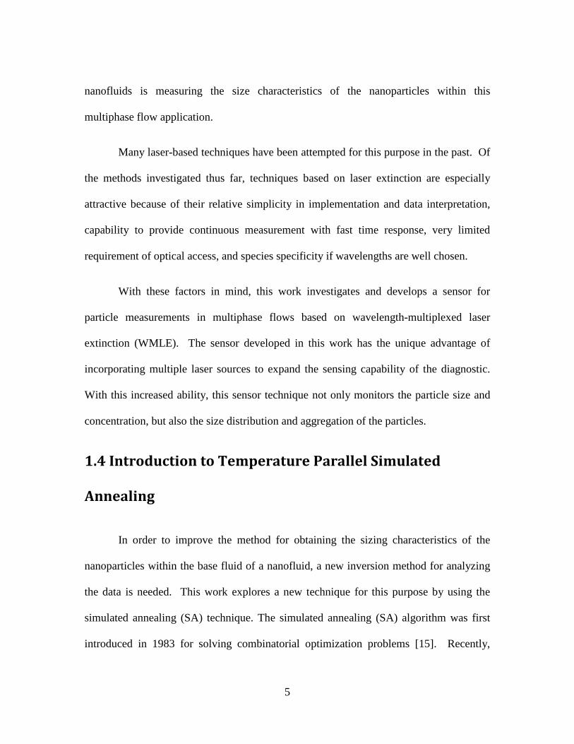
1.3 Introduction to Wavelength-Multiplexed Laser Extinction .....................................4
1.4 Introduction to Temperature Parallel Simulated Annealing ....................................5
1.5 Objectives of Dissertation ........................................................................................7
Chapter 2: Investigation of the Application of Phase Change Materials (PCM) ..........................................................................................................9
2.1 Abstract ....................................................................................................................9
2.2 Nomenclature .........................................................................................................10
2.3 Introduction ............................................................................................................12
2.4 Problem Formulation .............................................................................................14
2.5 The Physical Problem and the PCM Material Properties ......................................17
2.6 Numerical Analysis ................................................................................................20
2.7 Results and Discussion ..........................................................................................20
2.8 Conclusions and Discussion ..................................................................................27

v
Chapter 3: Development of a Sensor for Simultaneous Droplet Size and Vapor Measurement Based on Wavelength-Multiplexed Laser Extinction ...................................................................................29
3.1 Abstract ..................................................................................................................29
3.2 Introduction ............................................................................................................30
3.3 Theory ....................................................................................................................33
3.4 Droplet Measurement.............................................................................................37
3.4.1 Concept ...............................................................................................................37
3.4.2 Selection of Wavelengths ...................................................................................40
3.4.3 General WMLE for Droplet Measurement .........................................................44
3.5 Vapor Concentration Measurement .......................................................................47
3.5.1 Concept ...............................................................................................................47
3.5.2 Selection of Wavelengths ...................................................................................49
3.5.3 Differential Absorption and Wavelength Availability ........................................57
3.6 Summary ................................................................................................................58
3.7 Acknowledgement .................................................................................................58
Chapter 4: Investigation of Temperature Parallel Simulated Annealing for Optimizing Continuous Functions with Application to Hyperspectral Tomography.............................................................59
4.1 Abstract ..................................................................................................................59
4.2 Introduction ............................................................................................................60
4.3 Temperature Parallel Simulated Annealing ...........................................................63
4.4 Determination of Starting and Ending Temperatures ............................................66
4.5 Evaluation of Performance ....................................................................................69
4.6 Evaluation of Computational Cost .........................................................................73

vi
4.7 Preliminary Study of Exchange Frequency ...........................................................77
4.8 Application to Hyperspectral Tomography ...........................................................80
4.9 Summary ................................................................................................................86
4.10 Acknowledgements ..............................................................................................86
4.11 Appendix. Test Functions and Their Properties ..................................................87
Chapter 5: Conclusion .....................................................................................................92
References .........................................................................................................................94
vii
List of Tables
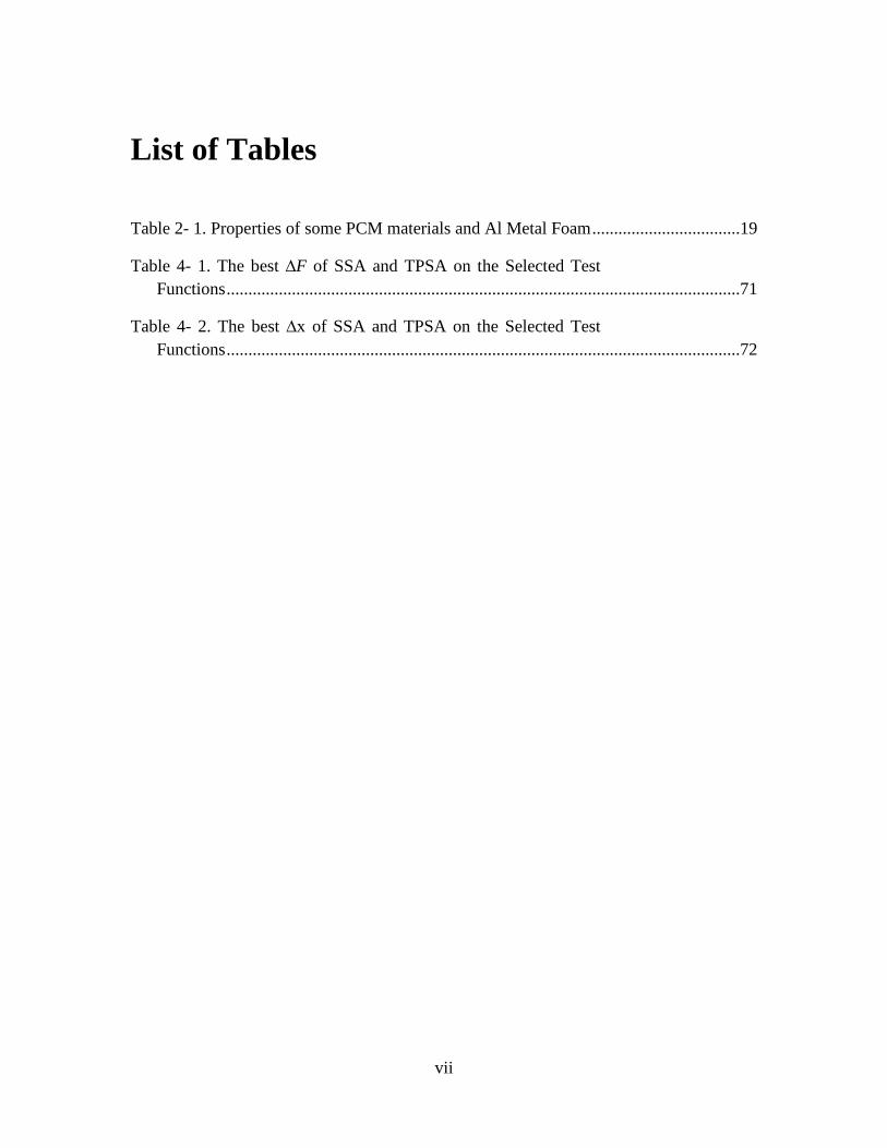
Table 2- 1. Properties of some PCM materials and Al Metal Foam ..................................19
Table 4- 1. The best ∆F of SSA and TPSA on the Selected Test Functions ......................................................................................................................71
Table 4- 2. The best ∆x of SSA and TPSA on the Selected Test Functions ......................................................................................................................72
viii
List of Figures
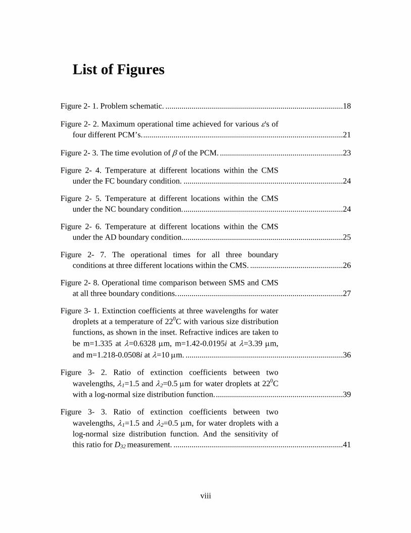
Figure 2- 1. Problem schematic. ........................................................................................18
Figure 2- 2. Maximum operational time achieved for various ε's of four different PCM’s. ...................................................................................................21
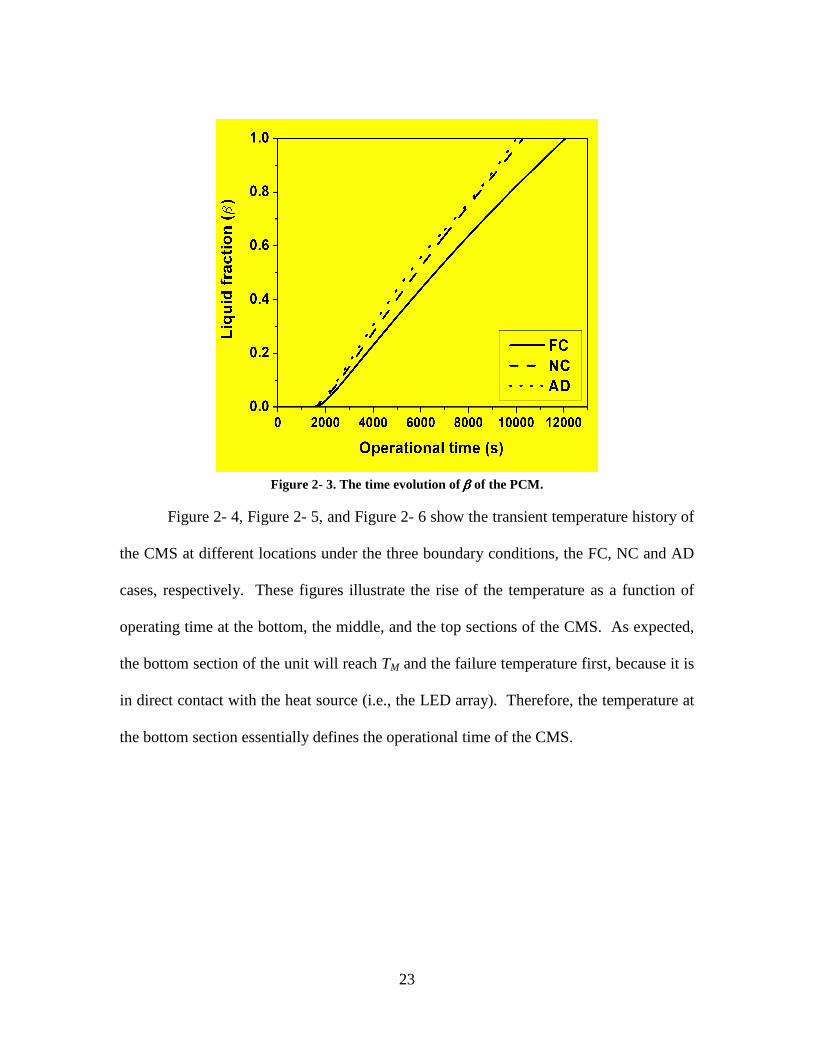
Figure 2- 3. The time evolution of β of the PCM. .............................................................23
Figure 2- 4. Temperature at different locations within the CMS under the FC boundary condition. ...............................................................................24
Figure 2- 5. Temperature at different locations within the CMS under the NC boundary condition. ...............................................................................24
Figure 2- 6. Temperature at different locations within the CMS under the AD boundary condition. ...............................................................................25
Figure 2- 7. The operational times for all three boundary conditions at three different locations within the CMS. ..............................................26
Figure 2- 8. Operational time comparison between SMS and CMS at all three boundary conditions. ..................................................................................27
Figure 3- 1. Extinction coefficients at three wavelengths for water droplets at a temperature of 220C with various size distribution functions, as shown in the inset. Refractive indices are taken to be m=1.335 at λ=0.6328 µm, m=1.42-0.0195i at λ=3.39 µm,
and m=1.218-0.0508i at λ=10 µm. ..............................................................................36
Figure 3- 2. Ratio of extinction coefficients between two wavelengths, λ1=1.5 and λ2=0.5 µm for water droplets at 220C with a log-normal size distribution function. ...............................................................39
Figure 3- 3. Ratio of extinction coefficients between two wavelengths, λ1=1.5 and λ2=0.5 µm, for water droplets with a log-normal size distribution function. And the sensitivity of this ratio for D32 measurement. ....................................................................................41

ix
Figure 3- 4. Ratio of extinction coefficients between two wavelengths (λ1=8.0 and λ2=0.5 µm) and the sensitivity of this ratio for D32 measurement with a log-normal size distribution function. Imaginary and real part of the refractive index at these wavelengths are assumed to change separately in the calculation. ...................................................................................................................44
Figure 3- 5. Schematic of differential absorption strategy for vapor measurement. ...............................................................................................................48
Figure 3- 6. Extinction coefficients for water droplets with different diameters and vapor absorbance from water vapor
from 0.5 to 9 µm at 220C. ............................................................................................50
Figure 3- 7. ∆Q for water droplet with different diameters when λ3
is selected at 5 µm. .......................................................................................................51
Figure 3- 8. Wavelength selection of differential absorption scheme for water with a temperature of 220C, total pressure 1 atm, mole fraction of water vapor 3%, and pathlength of 1cm. ...................................52
Figure 3- 9. Comparison of droplet extinction and vapor absorption at a wavelength of λ3=2.6705 µm for the evaporation process depicted in Figure 3- 10 to evaluate the applicable range of single wavelength scheme for vapor detection. Evaluation performed at a temperature of 220C, pressure 1 atm, and pathlength of 1 cm. ......................................................................................................54
Figure 3- 10. Comparison of differential droplet extinction and vapor absorption between the wavelengths chosen in Figure 3- 9 for the evaporation process depicted in Figure 3- 10 to evaluate the applicable range of the differential absorption scheme for vapor detection. Evaluation performed at a temperature of 220C, pressure 1 atm, and pathlength of 1 cm. ....................................56
Figure 4- 1. Illustration of the TPSA algorithm. ................................................................64
Figure 4- 2. Evolution of ∆F for both the SSA and TPSA algorithms. ...................................................................................................................65
Figure 4- 3. Determination of T0 and TN using the TC-curve. ............................................67

x
Figure 4- 4. Comparison of the SSA and TPSA algorithms on various test functions. ..................................................................................................73
Figure 4- 5. Computational time of the TPSA algorithm as a function of the exchange frequency. ............................................................................74
Figure 4- 6. The relationship between the speedup efficiency and the number of processes used in the TPSA algorithm. ................................................76
Figure 4- 7. Impact of the exchange frequency on the performance of the TPSA algorithm for the fRa10 and fS12 functions. ................................................78
Figure 4- 8. Impact of the exchange frequency on the performance of the TPSA algorithm for the fS4 and fRo5 functions. ...................................................79
Figure 4- 9. The mathematical formulation of the hyperspectral tomography problem. ...................................................................................................80
Figure 4- 10. Comparison of T phantom and reconstruction obtained using the TPSA algorithm. ............................................................................83
Figure 4- 11. Reconstruction obtained using the SSA algorithm in comparison to the phantom and that obtained using the TPSA algorithm. .....................................................................................................................85
Figure 4- 12. A plot of test function fG5 with respect to the first two variables (the other three variables are set to zero). .....................................................87
Figure 4- 13. A plot of test function fRa10 with respect to the first two variables (the other variables are set to zero). .......................................................88
Figure 4- 14. A plot of test function fB2. ............................................................................89
Figure 4- 15. A plot of test function fM5 with respect to the fourth and fifth variables (the first three variables are set to zero). ........................................90
Figure 4- 16. A plot of the fS2 test function. .......................................................................90
Figure 4- 17. A plot of the fR5 test function with respect to its first two variables (other variables are set to zero). ............................................................91
1
Chapter 1: Introduction
1.1 Motivation
The increased power demands in electric vehicles, especially when considering
the vehicles’ components, have hindered the progress of these vehicles. These increased
demands are especially difficult when considering the limited battery power available in
electric vehicles. Considering this limitation, many vehicle manufacturers are seeking to
decrease the overall power demand of each vehicle component, such as by using light
emitting diodes (LEDs) for their headlight systems. However, these new systems require
increased thermal protection, especially in outdoor environments. These increased
cooling needs demand more power for their individual thermal management systems.
Since this power is at a premium in electric vehicles, a method to thermally protect these
headlight systems is desired that requires little to no additional power draw for the
thermal management system. This thermal management system must be capable of
adequately cooling these component systems while maintaining packaging flexibility and
reliable operation in many environments.

2
Therefore, this investigation first explores the concept of adding a phase change
material (PCM) based heat sink for a LED headlight assembly. This strategy will utilize
the PCM’s natural phase change process in order to provide increased thermal protection
for this component, while demanding no additional power from the electric vehicle’s
system.
To further enhance the favorable aspects of this PCM based heat sink, the
application of nanoparticle suspended fluid (nanofluid) strategy is examined in this work.
These nanofluids have been shown in the past to increase the heat transfer capabilities of
the base fluid. The main challenge in accurately modeling this increase is that the sizing
characteristics of these particles must be known. Therefore, a new diagnostic tool is
needed for use in the study of multiphase flows. To address this issue, this work
investigates a new methodology based on laser extinction to detect the sizing
characteristics of particles in a multiphase flow. This methodology uses an optical
process with multiple wavelengths to provide increased information to detect the sizing
characteristics of the particles in multiphase flows.
One of the key issues in this methodology is the inversion process of the data in
order to retrieve the sizing characteristics. Therefore, a new algorithm is desired to solve
the inversion process to retrieve the sizing characteristics correctly. Therefore, the last
portion of this investigation seeks to develop an inversion method based upon the
simulated annealing (SA) algorithm. This inversion method, when implemented in a

3
parallelized fashion, has been shown to be able to solve the problem with high fidelity,
while reducing the normal computational cost of the SA algorithm.
1.2 Introduction to Phase Change Materials (PCMs)
PCMs have been extensively used in many engineering applications, including
building materials for energy storage improvement [1, 2], energy storage systems [1, 2],
electronics cooling systems [3-9], etc. One reason for the attractiveness of PCMs in such
extensive applications is that, due to its latent heat property, a PCM essentially behaves
as a thermal switch [10]. When the operation temperature of the target component
increases to the melting temperature of the PCM, the temperature of the system will
remain essentially steady until the PCM is completely melted. This phase change process
enables the absorption of a large amount of heat without increasing the temperature of the
electronic system being utilized. This process is a major consideration for choosing
PCMs as an alternative cooling technique in this work.
Another important reason why a PCM-based cooling strategy is particularly
attractive is the fact that the implementation of a particular PCM is relatively
straightforward. A PCM can easily be implemented into an existing thermal management
system because the latent heat property of the PCM is a natural process that does not
require any additional energy input from the system. Also, the PCM can be easily
implemented as a simple thermal block into an existing cooling system to provide added
thermal protection of critical components. For these reasons, the thermal properties of an
applicable PCM make it an attractive supplement to factory installed cooling strategies.

4
Of important interest is the role that the thermal conductivity of the PCM plays in
the cooling system’s performance [10]. In particular, organic PCMs exhibit many
qualities needed in component cooling, including high latent heat, non-corrosiveness, etc.
[1, 2, 10], but they also exhibit a prohibitively low thermal conductivity [1, 2, 10] to be
used in practical thermal management systems. To overcome this limitation of low
thermal conductivity, it has been the focus of many recent research efforts, including this
work, to suggest suspending these PCMs in a metal foam matrix [4, 11-14] in order to
increase the effective thermal conductivity of the suspension. In conjunction with the
increase of the thermal conductivity of the PCM based heat sink, an optimization process
for the selection of the optimal porosity of the PCM utilized must be performed that
considers both the increase in thermal conductivity and loss of latent heat of the PCM in
order to provide the maximum operational time in any system. Considering these factors,
this work not only will explore the applicability of using a PCM in a proposed thermal
management system, but also will find the optimal volume fraction of the proposed PCM
to be utilized for an LED lighting system.
1.3 Introduction to Wavelength-Multiplexed Laser
Extinction
To increase the effectiveness of the favorable aspects of PCMs discussed in the
previous section, a strategy implementing nanofluids is also considered because of their
increased heat transfer characteristics. One of the limiting factors in the study of
5
nanofluids is measuring the size characteristics of the nanoparticles within this
multiphase flow application.
Many laser-based techniques have been attempted for this purpose in the past. Of
the methods investigated thus far, techniques based on laser extinction are especially
attractive because of their relative simplicity in implementation and data interpretation,
capability to provide continuous measurement with fast time response, very limited
requirement of optical access, and species specificity if wavelengths are well chosen.
With these factors in mind, this work investigates and develops a sensor for
particle measurements in multiphase flows based on wavelength-multiplexed laser
extinction (WMLE). The sensor developed in this work has the unique advantage of
incorporating multiple laser sources to expand the sensing capability of the diagnostic.
With this increased ability, this sensor technique not only monitors the particle size and
concentration, but also the size distribution and aggregation of the particles.
1.4 Introduction to Temperature Parallel Simulated
Annealing
In order to improve the method for obtaining the sizing characteristics of the
nanoparticles within the base fluid of a nanofluid, a new inversion method for analyzing
the data is needed. This work explores a new technique for this purpose by using the
simulated annealing (SA) technique. The simulated annealing (SA) algorithm was first
introduced in 1983 for solving combinatorial optimization problems [15]. Recently,

6
many research efforts have been devoted to successfully demonstrating its use in solving
both discrete [16, 17] and continuous optimization problems [18-23], revealing several
critical advantages of the use of the SA algorithm over other optimization techniques.
For example, the SA algorithm can optimize complicated problems with a large number
of variables and numerous confusing local minima. In addition, the SA algorithm is
insensitive to the initial guess, which is especially important when no a priori
information about the solution is available. Because of these advantages, the SA
algorithm shows great promise in solving the sizing characteristics of nanoparticles
within a base fluid.
On the other hand, the disadvantages of the SA algorithm are also well-
recognized. One of the primary disadvantages of the SA algorithm is its high
computational cost [20, 23]. Many research efforts have focused on developing variants
of the SA algorithm to reduce the computational cost [24-26] by either optimizing the
annealing schedule [16, 27-30], or by parallelizing the SA algorithm [25, 31-34].
However, the optimization of the annealing schedule is usually problem-dependent [27,
28], and therefore limits the applicability of the results from these efforts. For the
parallelization of the SA algorithm, convergence is not guaranteed, and the maximum
speedup efficiency is very limited [33, 34].
Considering these limitations of the SA algorithm and the subsequent methods to
overcome them, this work studies the application of the temperature parallel simulated
annealing (TPSA) algorithm, which combines the well-established parallel tempering (or
7
replica exchange) method [35, 36] and the SA algorithm [37]. The TPSA algorithm
overcomes the above limitations by theoretically guaranteeing convergence; increasing
the speedup of the parallelization process; and, because the TPSA optimization process
occurs at constant temperature, not requiring an annealing schedule [25, 32, 38].
However, the limiting factor to the application of the TPSA algorithm is the fact
that this algorithm has only been studied primarily on discrete functions in previous
efforts [16, 32, 33, 37, 39]. Therefore, this work conducts a systematic study of the
TPSA algorithm on continuous functions that would be applicable to the purpose of this
work.
1.5 Objectives of Dissertation
The first objective of this work is to explore the application of PCMs to an
existing thermal management system in order to ensure increased thermal protection of a
LED headlight assembly. Our studies have found that the use of specific PCMs shows
promising results in extending the operational time of these components, especially when
used in conjunction with metal foam suspensions in order to increase the thermal
conductivity of the PCM being used. Also, our results have potentially established a
procedure to optimize the volume fraction of the PCM in order to optimize the
operational time.
The next objective of this work is to develop an optical technique combined with
an inversion method applicable to multiphase flow applications in order to obtain the

8
sizing characteristics of nanoparticles within a nanofluid. The development of these two
concepts will enable further understanding of the application of nanofluids to the thermal
management system using PCMs. Our studies have demonstrated that the WMLE
method can effectively measure the size of particles in multiphase environments.
Furthermore, our studies have shown that the implementation of a new inversion
algorithm based upon simulated annealing (SA) in a parallelization environment can
analyze the data obtained accurately under acceptable computational cost.
This work is based upon the work completed and published in three peer-
reviewed journal articles; therefore, the rest of this work is organized as follows. In
Chapter 2, the journal article that explores the application of PCMs to a LED headlight
system is presented. Chapter 3 contains the journal article that pursues the development
of the WMLE method for measuring particle/droplet sizes. Then, Chapter 4 presents the
journal article that develops the TPSA algorithm. The final chapter summarizes the work
that is contained within this dissertation.

9
Chapter 2: Investigation of the
Application of Phase Change Materials
(PCM)
2.1 Abstract
Phase change materials (PCMs) are extensively used in many engineering areas
for thermal management purposes. This paper investigated the application of PCMs for
vehicular systems, especially for the thermal protection of vehicle lighting systems based
on light emitting diodes (LEDs). Lighting systems based on LEDs offer many
advantages, however, also pose a smaller margin of error for thermal management. This
paper analyzed the combined use of PCMs with metal foam for cooling systems. The
cooling performance was studied numerically under different porosity values of the metal
foam, and different boundary conditions. The cooling performance was also compared to
a solid metal sink system (SMS) and was found to offer several distinct cooling
characteristics.

10
2.2 Nomenclature
b = half thickness of bump in hexagonal structure of metal foam
CMS = cooling management system
SMS = solid management system
T = temperature
TM = melting temperature of PCM
TS = solidus temperature of PCM
TL = liquidus temperature of PCM
D = Diameter of CMS and SMS unit
H = height of CMS and SMS unit
h = convective heat transfer
Q = heat added to system
CP = specific heat at constant pressure
CPeff = combined effective specific heat of conductor and PCM
(ρCP)MF = (ρCP) of the metal foam
(ρ�CP)PCM = (ρCP) of the PCM
k = thermal conductivity
kMF = thermal conductivity of the metal foam
ks = thermal conductivity of solid metal foam
kf= thermal conductivity of PCM at its respective solid or liquid phase
kPCM = thermal conductivity of the PCM

11
keff = combined effective thermal conductivity of conductor and PCM
r = area ratio of the solid fiber to void area
href = reference enthalpy
hsens= sensible enthalpy
Tref = reference temperature
L = latent heat
Lf = half length of fiber of metal foam
Sh = source term to correct the latent heat variation during the melting process
∆H = heat of fusion
Htot = total enthalpy of material
∆t = time step
FC = forced convection condition
NC = natural convection condition
AD = Adiabatic condition
Greek Symbols
ρ = density
ρMF = density of the metal foam
ρPCM = density of the PCM
ρeff = effective density
ε = volume fraction of the PCM
β = liquid fraction

12
2.3 Introduction
Phase change materials (PCMs) are extensively used in many engineering
applications. They are used in energy storage systems [40], electronics cooling systems
[41], building materials for energy storage improvement [42], heat exchangers [43], and
many other similar applications. This paper investigated the applications of PCMs for the
thermal management in vehicular systems, especially the thermal management of vehicle
lighting systems based on light emitting diodes (LEDs). Lighting systems based on LEDs
offer many advantages, including improved energy efficiency and potential for weight
reduction. However, such lighting systems also pose a smaller margin of error for
thermal management because LEDs can be permanently damaged if their operation
temperature exceeds a critical temperature. Furthermore, the output power of LEDs
varies significantly with the operation temperature. Therefore, a better thermal
management technique is desired for such light systems.
A cooling management system (CMS) based on PCMs appear very attractive for
this purpose because a PCM essentially behaves as a thermal switch. When the operation
temperature of the lighting systems begins to exceed that of the melting temperature of
the PCM, the temperature of the system stops increasing until the PCM is completely
melted. Therefore, CMS based on PCMs show good promise to tightly control the
temperature of LEDs. But as described above, the operation time of the CMS is
fundamentally limited by the melting time of the PCM, which was a key parameter to be

13
investigated in this study. The investigation was focused on maximizing the operation
time of the CMS while still operating under specified sizing and other restraints.
More specifically, PCMs are characterized by their TM, ∆H, and their TS and TL
(Other properties may need to be considered for specific applications, e.g., ρ, chemical
stability, safety, and flammability [44]). Once the operating temperature of the system
being cooled reaches the TL of the PCM, the PCM begins to melt and stores the thermal
energy that the system releases during this process. The amount of thermal energy that
the PCM can store depends on its ∆H and amount. During the melting process, the PCM
and, therefore, the system temperature remain constant. The duration of the melting
process delays the system from reaching its maximum operational temperature, which
prolongs the operational time of the system where the operational time is defined as the
amount of time it takes for the system to reach its maximum operational temperature.
This operational time gain depends heavily on the PCM mass ratio and the PCM
thermophysical properties k, ρ, ∆H, TM, and CP. The configuration of the unit containing
the PCM, such as the thermal properties and the distribution of a thermal conductivity
enhancer that encapsulates the PCM, also affects the system’s performance [45, 46].
It is known that the PCM’s conductivity plays a very important role in the cooling
system’s performance [45]. Higher conductivity is usually preferred, because it aids in
heat distribution, more uniform PCM melting process, and overall effectiveness of the
CMS. Consequently, a higher conductivity of the PCM would increase the heat transfer
rate and prolong the operational time of the lighting system. However, many PCMs have

14
relatively low conductivity. For example, organic PCMs exhibit relatively low thermal
conductivity, even though they, in comparison with metallic PCMs, are less corrosive,
more readily available, and less costly. In order to improve the overall effective
conductivity of the CMS to leverage the advantages of such organic PCMs, many
researchers suggest filling the PCM into a honeycomb structure or mixing it with metal
foam conductors [46, 47]. However, with a fixed size for the CMS unit, increasing the
effective conductivity of the system will decrease the effective mass of the PCM material.
This, in turn, reduces the heat storage potential of the system, thereby, reducing the
operational time of the lighting system. Hence, this paper analyzed the optimal volume
fraction of the PCM for attaining the maximum operational time at a fixed size for the
CMS unit.
2.4 Problem Formulation
During the phase change process (melting or solidification), the PCM
encapsulated in a porous material, in this case, metal foam (MF), can exist in three states:
solid, liquid, and a two phase mixture. Additionally, the thermal properties of a PCM-
MF matrix are different from the constituent properties. To simplify the mathematical
model, the PCM–MF combination can be treated as a body of uniform equivalent
physical and thermal properties—principally CP, ρ and k of the PCM and MF. The
effective properties of the mixture are calculated based on the volume ratio, ε of the PCM
material in the mixture, as follows:

15
( ) [(1- )( ) ( ) ] /P eff P MF P PCM effC C Cε ρ ρ ρ= + (2.1)
where
=(1- )eff MF PCMρ ε ρ ε ρ+ (2.2)
and as derived in [48],
( )( )( )( )
( )( )( )( )( )
( )( )( )
1
1 3 1
12
2 33
3 2
4 3 3
f
f f s f
f
eff
f f s f
f
f f s f
r b L
k b L k k
r b Lk
k b L k k
b L
k r b L k k
− + + − − = + + − −
+ + −
(2.3)
where b/Lf is given by the following expression
( )2 2 41 2 1
3 3
2 42 1
3 3f
r r rb
Lr
ε
− + + − − + =
− +
(2.4)
Or, in a more simplified yet reasonably accurate form, keff can be calculated as
follows [49]:
=(1- )eff MF PCMk k kε ε+ (2.5)

16
This analysis performed in the paper was based on Equation (2.5). Also, instead
of tracking the liquid-solid front explicitly, the enthalpy-porosity formulation can be used
in this type of application. The two phase zone is treated as a porous zone with porosity
equal to β, the liquid fraction, which is defined in the following Equation (2.6):
0 if
if
1 if
s
ss l
l s
l
T T
T TT T T
T T
T T
β
β
β
= <
−= < <
−
= >
(2.6)
With this definition (also referred to as the lever rule [50]), an enthalpy-porosity
technique can be used for modeling the melting process [46]. The two phase zone is a
region in which β of the PCM lies between 0 and 1, with 1 corresponding to the PCM
being fully melted and 0 corresponding to the PCM being fully solid. The two phase
zone is modeled as a “pseudo" porous medium in which the porosity decreases from 1 to
0 as the material melts. When the material has fully melted in the cell, the porosity
becomes 0.
The enthalpy of the material is computed as the sum of hsens, and ∆H:
tot sensH h H= + ∆
(2.7)
where
ref
T
sens ref pTh h c dT= + ∫
(2.8)

17
The latent heat content of the PCM (a mixture of melted liquid and unmelted
solid), L, can now be written in terms of L and β as follows:
H Lβ∆ = (2.9)
Obviously, the latent heat content, L, varies between zero (for a pure solid) and L (for a
liquid).
For solidification/melting problems, the energy equation can be written as [50]
( ) ( )P hC T t k T Sρ∂ ∂ = ∇ ⋅ ∇ + (2.10)
where Sh is the source term to account for the latent heat variation during the melting
process. It is represented by:
( )hS H tρ= − ∂ ∆ ∂ (2.11)
And ∆H is calculated utilizing the lever rule from Equation (2.6).
Now, temperature can be solved for by the interaction between the energy
equation and the liquid fraction equation.
2.5 The Physical Problem and the PCM Material Properties
The physical problem was defined according to the design constraints of an LED
light system. The heat input from the vehicle’s lighting system was given to be a total of
73.5 W. The maximum permissible temperature of the lighting system was not to exceed

18
90oC and the ambient temperature was given to be 27oC. The problem is assumed to be
conduction-dominated within the CMS unit, thus the internal natural convective heat
transfer effect of the PCM can be neglected.
The geometry of the CMS consisted of a cylindrical container of aluminum
material. The container contains a mixture of a PCM suspended in an aluminum metal
foam. Figure 2- 1 shows the sketch of the CMS unit. The diameter (D) and height (H) of
the domain were 10 cm and 10 cm, respectively.
Three operating conditions were considered in this investigation, by assuming
three different boundary conditions. In the first case the unit is assumed to be fitted
outside the engine-hood, exposed to an ambient temperature of 27oC, and air velocity of
40 kilometers per hour (the average speed of the vehicle). This gave an average
convective heat transfer coefficient of 14 W/m2-K. This case was considered to be the
forced convection (FC) condition.
Figure 2- 1. Problem schematic.
D
H
Q
PCM suspended in metal foam
Line of symmetry
Bottom Middle Top
Al container

19
In the second case the unit is assumed to be installed outside the engine-hood, but
with the vehicle at rest. In this case, the temperature that the unit was exposed to is the
ambient temperature of 27oC. Natural convection would be present in this case,
therefore, a value of h = 5 W/m2-K was then determined. This case was considered to be
the natural convection (NC) condition.
Material ρ [kg/m3] C
P [J/kg-K] ∆H [J/kg] T
M [
oC]
MF: Al 2700 963 - -
PCM: Climsel
C 70 1700 3600 280800 70
PCM: Therma-sorb-175 930 2000 200000 79
PCM: RT80
920 2400 175000 81
PCM: Triacontane
810 2050 251000 65
Table 2- 1. Properties of some PCM materials and Al Metal Foam
Finally, the third case assumed the unit was to be installed under the engine-hood.
The temperature of the environment under the hood (engine temperature) would be
extremely high, much higher than the maximum allowable temperature of the protected
lighting system. Thus, the unit must be completely isolated. This is considered to be the
worst operating condition possible, since the unit is operating without any external
cooling. This case was considered to be the adiabatic (AD) condition.
The thermophysical properties of the PCM and the aluminum metal foam used in
this study are listed in Table 2- 1, and are assumed to remain constant over the entire
temperature range encountered in the operation.

20
2.6 Numerical Analysis
The commercially available software programs Fluent and ANSYS were used to
perform a control-volume-based technique that converts the governing equations into
algebraic equations to be solved. This control-volume technique consisted of integrating
the governing equations about each control-volume, yielding discrete equations that
conserve each quantity on a control-volume basis [51].
A point implicit (Gauss-Seidel) linear equation solver was used in conjunction
with an algebraic multigrid (AMG) method to solve the resultant scalar system of
equations for the dependent variable in each cell.
For transient simulations, the governing equations were discretized in both space
and time. Temporal discretization involved the integration of every term in the
differential equations over a time step ∆t.
A fully implicit integration scheme was used for integration of the unsteady term
(i.e., using “the future time level”). The advantage of the fully implicit scheme is that it
is unconditionally stable with respect to the time step size. A grid-independence study
was carried out to test the sensitivity of the solution to the grid size.
2.7 Results and Discussion
It is very important to select a PCM with a TM that is close to the maximum
allowable temperature of the protected system to attain its best performance [52].

21
According to our survey, the PCMs listed in Table 2- 1 are among the most suitable
organic PCMs which satisfy the above condition for the thermal management of the LED
lighting system.
Use of a different PCM involves a tradeoff among various factors, e.g., the
cooling effectiveness, the operational time, and the thermal protection. For example, as
can be seen, ClimSel C70 clearly has the highest ∆H, k, and (ρCP). However, its TM is too
low when compared with the target protection temperature (90 0C), which will be
overprotective in practice. Thermasorb-175 and RT80 have a much closer TM to that of
the failure temperature of the lighting system. However, these two (along with RT80)
have much lower values for (ρ CP) and ∆H.
Figure 2- 2. Maximum operational time achieved for various εεεε's of four different PCM’s.
In this study, all four PCMs were tested over a range of volume fractions in order
to see which PCM can give the longest operational time for the lighting system. The

22
results of this investigation were plotted in Figure 2- 2. Figure 2- 2 clearly shows that all
four PCM-MF mixtures yield about the same duration of operational time at a volume
fraction of ε = 0.75.
Figure 2- 2 also indicates that ClimSel C70 yielded the longest operational time in
comparison with the rest of PCMs. Therefore, ClimSel C70 was chosen for the rest of
the study to be discussed below.
To illustrate the operation of the CMS more closely, we calculated the liquid
fraction (β) at different operational times. Time zero was defined as the time when the
LEDs were turned on to generate a heat flow (Q) of 73.5 W. Figure 2- 3 shows the
variation of β versus the operational time of the PCM-MF mixture at the three types of
boundary conditions as mentioned above: the forced convection, FC, the natural
convection, NC, and the adiabatic, AD. Figure 2- 3 shows that under all boundary
conditions, the PCM was fully melted after a certain duration of operation under the
given conditions (heat load, driving velocity, geometry of the CMS, etc.). As expected,
the FC boundary conditions corresponded to the longest melting time (~ 12,000 seconds
in this case), which defines the operational time of the CMS. Under the AD boundary
condition, heat transfer out of the system is zero. Thus, the time needed to melt the PCM
was the shortest. It is desirable to prolong the operational time, and one possible strategy
involves using a different geometry of the CMS.
23
Figure 2- 3. The time evolution of ββββ of the PCM.
Figure 2- 4, Figure 2- 5, and Figure 2- 6 show the transient temperature history of
the CMS at different locations under the three boundary conditions, the FC, NC and AD
cases, respectively. These figures illustrate the rise of the temperature as a function of
operating time at the bottom, the middle, and the top sections of the CMS. As expected,
the bottom section of the unit will reach TM and the failure temperature first, because it is
in direct contact with the heat source (i.e., the LED array). Therefore, the temperature at
the bottom section essentially defines the operational time of the CMS.

24
Figure 2- 4. Temperature at different locations within the CMS under the FC boundary condition.
Figure 2- 5. Temperature at different locations within the CMS under the NC boundary condition.

25
Figure 2- 6. Temperature at different locations within the CMS under the AD boundary condition.
Figure 2- 7 summarizes the time at which the critical temperature was reached
under different boundary conditions at different locations. As can be seen, under the FC
condition, the most favorable cooling condition, the bottom section reached the critical
temperature after 13,490 seconds (3.7 hours) of operation; under the NC condition, the
bottom section reached the critical temperature after 11240 seconds (3.1 hours) of
operation; and finally, under the AD boundary condition, after 10790 seconds (2.99
hours) of operation.
Again, one possible approach to prolong the operational time of the CMS
involves varying the geometry of the CMS. Enlarging the size of the CMS represents a
simple, yet effective method. For example, our calculations showed that with a unit size
of 20 cm diameter and 20 cm height, an operational time of 18 hours can be obtained

26
under the FC boundary condition. Research is underway to optimize the operational time
under various geometrical constraints.
Figure 2- 7. The operational times for all three boundary conditions at three different locations
within the CMS.
Lastly, we compared the distinct cooling characteristics between the PCM-based
method and the method based on a solid metal sink system (SMS). Figure 2- 8 compares
the history of temperature rise at the bottom section using the PCM-based method (the
CMS case) and the cooling method based on a solid unit of aluminum (the SMS case). In
this comparison, both the CMS and the SMS cases were assumed to have the same
geometry as defined in Figure 2- 1; and both cases were assumed to operate under the
same conditions as defined previously. As Figure 2- 8 shows, with the SMS system,
temperature increased monotonically until it reached an asymptotic value (corresponding
to the steady state value). In contrast, with the CMS system, temperature first increased
to the melting temperature of the PCM, then remained almost constant around the melting

27
temperature, and finally started increasing again after the PCM was completely melted.
This difference clearly elucidates the functionality of the PCM system as a thermal
switch to tightly control the temperature.
Figure 2- 8. Operational time comparison between SMS and CMS at all three boundary conditions.
2.8 Conclusions and Discussion
The use of PCMs was investigated for the thermal management of LED lighting
systems. The advantages of the PCMs to tightly control temperature below the failure
temperature of the LEDs were clearly illustrated. The performance and limitations of the
PCM-based cooling methods for such applications were examined using extensive
numerical simulations. The use of metal foam significantly improved the cooling
performance, and the optimal MF fraction was determined. The cooling performance
was also compared to a solid metal sink system and was found to offer several distinct
cooling characteristics.

28
Two conclusions can be drawn from this study. First, a well-chosen PCM
provides better control of temperature when compared with a metallic heat sink. Second,
the operational time of the PCM-based method depends sensitively on several factors,
especially the size and geometry of the cooling unit. Research is underway to optimize
the design of PCM-based cooling systems under geometrical constraints.
Current ongoing research involves investigating the performance of the PCM-
based cooling systems under more realistic boundary conditions, and validating the
numerical analysis via experimental tests. In reality, the boundary conditions are
characterized by mixed modes of heat transfer, and transient temperatures. Though the
rigorous is undergoing, many insights can be obtained from the results presented here.
For example, the case with an adiabatic boundary condition represents the worst scenario
under a constant under-hood temperature. When the temperature fluctuates (as long as it
does not exceed the temperature studied here), the operational time will be prolonged. A
prolonged operational time can also be expected when mixed modes of heat transfer are
considered.

29
Chapter 3: Development of a Sensor for
Simultaneous Droplet Size and Vapor
Measurement Based on Wavelength-
Multiplexed Laser Extinction
3.1 Abstract
Multiphase flows involving liquid droplets in association with a gas flow occur in
many industrial and scientific applications. Recent work has demonstrated the feasibility
of using optical techniques based on laser extinction to simultaneously measure vapor
(e.g., vapor concentration and temperature) and droplet properties (e.g., droplet size and
loading). This work introduces the theoretical background for the optimal design of such
laser extinction techniques, which is termed the WMLE (wavelength-multiplexed laser
extinction) technique in this paper. After a brief survey of past work, this paper focuses
on the development of WMLE and presents a systematic methodology to guide the
selection of suitable wavelengths and therefore optimize the performance of WMLE for a

30
specific application. WMLE schemes utilizing wavelengths ranging from 0.5 to 10 µm
are illustrated for droplet size and vapor concentration measurements through an example
of water spray and are found to enable unique and sensitive Sauter mean diameter
measurement in the range of ~1 to 15 µm along with accurate vapor detection. A vapor
detection strategy based on differential absorption is developed to extend accurate vapor
measurement to a significantly wider range of droplet loading and vapor concentration
compared with strategies based on direct fixed-wavelength absorption. Expected
performance of the sensor is modeled for an evaporating spray. This work is expected to
lay the groundwork for implementing optical sensors based on WMLE in a variety of
research and industrial applications involving multi-phase flows.
3.2 Introduction
In many scientific and industrial applications, multiphase problems exist in the
form of liquid droplets in association with a gas flow. The study of vaporization or
condensation of liquid droplets inside a spray is one typical example. In such
applications, it would be desirable to monitor both the vapor and the droplets
simultaneously.
Numerous laser-based techniques have been developed for the separate
characterization of either vapor or droplets. These vapor sensing techniques include laser
Rayleigh scattering [53], spontaneous Raman spectroscopy [53], laser-induced
fluorescence (LIF) [53, 54], spectrally-resolved absorption [55], and others. Droplet
31
measurement techniques include the measurement of Fraunhofer diffraction of laser
radiation by droplets [56], laser phase Doppler anemometry [57], laser extinction [58,
59], and wavelength-multiplexed laser extinction [60]. Each technique has its own
advantages and disadvantages and is useful for a certain domain of applications.
However, these techniques are generally not transferable to the simultaneous
monitoring of both vapor and droplet properties. Some vapor sensing techniques based on
elastic scattering such as the Rayleigh scattering technique or LIF can be extended to
measure both vapor and droplets. However, usually the scattering from droplets greatly
exceeds that from the vapor, therefore, jeopardizing or even prohibiting an accurate vapor
measurement. Similar reasoning precludes the direct combination of one vapor and one
droplet measurement technique discussed above for simultaneous vapor and droplet
measurements. Furthermore, different techniques usually have different temporal and
spatial resolution, and some of the techniques may require wide optical access, so that
practical implementation becomes difficult.
Despite these challenges, a few laser-based diagnostic techniques have been
attempted for simultaneous characterization of vapor and droplets. Laser Induced
Exciplex Fluorescence (LIEF) developed by Melton [61] allowed two-dimensional
imaging of vapor and droplets simultaneously under limited conditions. Besides
implementation difficulties, however, the LIEF signal is difficult to quantify, and
quenching from oxygen limits most of the LIEF applications to nitrogen environments
[53]. For more quantitative and realistic applications, Chraplyvy and Tishkoff [62, 63]

32
proposed and applied a method based on a two-wavelength laser extinction strategy to
measure vapor concentration and droplet volume fraction simultaneously in an
evaporating fuel spray. This technique requires an independent droplet size distribution
(or droplet size in the case of mono-dispersed droplets) measurement, and the dynamic
range of measurements offered by this technique was limited.
Of the methods investigated thus far, techniques based on laser extinction are
especially attractive owing to their relative simplicity in implementation and data
interpretation, capability to provide continuous measurement with fast time response,
very limited requirement of optical access, and species specificity if wavelengths are well
chosen. This paper describes the development of a sensor for simultaneous droplet and
vapor measurement based on wavelength-multiplexed laser extinction (WMLE). The first
unique feature of this sensor involves the incorporation of laser sources at an arbitrary
number of wavelengths to expand sensing capability of the diagnostic to more quantities
besides vapor concentration and droplet volume fraction. The second unique feature
involves a vapor sensing technique modified from spectrally-resolved absorption, namely
differential absorption, to significantly improve the detection limit of vapor sensing.
Experimental demonstration and application of the sensor have been reported elsewhere
[64, 65]. Here we describe the sensing strategy and analyze the sensor performance.
Systematic methodologies are developed to guide the selection of wavelengths to achieve
optimized performance for both vapor and droplets measurement, and expected
performance is modeled for an evaporating spray.

33
3.3 Theory
When a collimated light beam at wavelength λ is incident upon a mixture of vapor
and droplets, the transmitted beam intensity (It) is related to the incident beam intensity
(I0) by
0( ) /
exp[ ( )] exp[ ( )]
exp[ ( ) ] exp[ ( )]
t
vapor drops
drops
T I I
X P L
λ
τ λ τ λ
α λ τ λ
=
= − ⋅ −
= − ⋅ ⋅ ⋅ ⋅ −
(3.1)
where:
T(λ) = the optical transmittance at wavelength λ
τvapor(λ) = the vapor absorbance
τdrops(λ) = the droplet extinction
α(λ) = the absorption coefficient of vapor (cm-1·atm-1)
X = the vapor mole fraction
P = the total (mixture) pressure along the pathlength (atm)
L = the pathlength (cm)
From light scattering theory [66], extinction by a collection of monodisperse
spherical droplets is related to the number density and size of the droplets in the
following equation
2
( / , )4drops n
DC Q D m L
πτ π λ= ⋅ ⋅ ⋅ (3.2)

34
where:
Cn = the number density of the droplets (cm-3)
D = diameter of the droplets (cm)
Q(πD/λ,m) = the extinction coefficient of a droplet with diameter D at
wavelength λ
m = the complex refractive index of the droplets at wavelength λ
Q(πD/λ,m) is a complex function of the incident wavelength and droplet diameter
and calculation of Q(πD/λ,m) requires numerical methods, except in some special cases.
This work uses a Mie scattering algorithm described in [67] to compute the droplet
extinction coefficients. In the case of a collection of poly-dispersed droplets, Equation
(3.2) needs to be modified as
2
0
( / , ) ( )4drops nC L Q D m f D D dDπ
τ π λ∞
= ∫ (3.3)
where f(D) is the droplet size distribution function defined such that 0
( ) 1f D d D∞
=∫ ,
and f(D)dD represents the probability that a droplet has diameter between D and D+dD.
Due to the lack of fundamental mechanism or model to build droplet size distribution
functions theoretically, various distribution functions have been used based on
probability analysis or empirical observations. A log-normal function, defined as
following, is one of the most commonly used distribution functions:

35
22
1 1( ) exp[ (ln ln ) ]
2(ln )2 lnCMf D D D
D σπ σ= − ⋅ − (3.4)
In this equation, σ represents the standard deviation of the distribution
(distribution width); and DCM the count median diameter, which means 50% of the
droplets in the distribution have diameter smaller than DCM and 50% larger than DCM.
In many calculations and applications, it is convenient to restrict the work to
averaged parameters instead of using the complete size distribution function. Based on
f(D), many statistical parameters about the droplet distribution can be defined. Two
useful parameters, the mean scattering coefficient ( )Q and the Sauter Mean Diameter
(D32), are defined as following
2
0
2
0
( / , ) ( )
( )
Q D m f D D dDQ
f D D dD
π λ∞
∞= ∫∫
(3.5)
3
032
2
0
( )
( )
f D D dDD
f D D dD
∞
∞= ∫∫
(3.6)
Obviously, for a given droplet distribution, Q depends on the incident wavelength
and some characteristic diameter of the droplets. D32 is used as such a characteristic
diameter in this paper and this dependence is denoted as 32( / , )Q D Dπ λ . Figure 3- 1
provides some example calculations to show the variations of Q (for mono-dispersed
droplets) and Q (for poly-dispersed droplets) with droplet size at three wavelengths for
water droplets. In the case of poly-dispersed droplets, size distribution functions are taken

36
to be the log-normal function defined in Equation (3.4) with different distribution widths,
as illustrated in the insert of Figure 3- 1. Refractive indices used in the calculations
shown in Figure 3- 1 are from measurements made in [68, 69]. An important observation
is that the positions of principal maxima of the extinction coefficient curve display only a
weak dependence on the width (σ) of the log-normal distribution functions. Furthermore,
a weak dependence on the distribution functions is found both in our work and in studies
elsewhere [58], especially when the distribution width (characterized by the standard
deviation of the distribution function) is large. Also, note the insensitivity of extinction
coefficients to distribution width at a wavelength of 10 µm.
Figure 3- 1. Extinction coefficients at three wavelengths for water droplets at a temperature of 220C
with various size distribution functions, as shown in the inset. Refractive indices are taken to be m=1.335 at λλλλ=0.6328 µµµµm, m=1.42-0.0195i at λλλλ=3.39 µµµµm, and m=1.218-0.0508i at λλλλ=10 µµµµm.
Finally, by introducing a new parameter, the droplet volume fraction CV, Equation
(3.2) and (3.3) can be transformed into the following forms

37
3 ( / , )
2V
drop
C Q D m L
D
π λτ = for mono-dispersed droplets (3.7)
and
32
32
3 ( / , )
2V
drop
C Q D m L
D
π λτ = for poly-dispersed droplets (3.8)
where CV is defined as the volume fraction occupied by liquid droplets along the
pathlength, and can be calculated by the following equations
3
6V nC C Dπ
= ⋅ for mono-dispersed droplets (3.9)
and
3
0( )
6V nC C D f D dDπ∞
= ∫ for poly-dispersed droplets (3.10)
3.4 Droplet Measurement
3.4.1 Concept
At wavelengths where vapor does not absorb (i.e. α(λ) = 0), the optical
transmittance is only due to droplet extinction and is given by
( ) exp[ ( )]dropsT λ τ λ= − (3.11)

38
where τdrops(λ) is given by Equation (3.7) or (3.8).
Transmittance measurement at one wavelength is not sufficient to extract droplet
information because of the multiple unknowns (Cn and D) in Equation (3.11). If
transmittance measurements are performed at multiple wavelengths (e.g. λ1 and λ2), then
from Equation (3.7) and (3.8) we obtain
1 1
2 2
( ) ( / , )
( ) ( / , )drops
drops
Q D mR
Q D m
τ λ π λτ λ π λ
= = for mono-dispersed droplets (3.12)*
and
1 32 1
2 32 2
( ) ( / , )
( ) ( / , )drops
drops
Q D mR
Q D m
τ λ π λτ λ π λ
= = for poly-dispersed droplets (3.13)*
Equations (3.12) and (3.13) state that the ratio of measured extinction at
wavelength λ1 and λ2 only depends on droplet size (or size distribution function) and
equals the ratio of extinction coefficients (R) at these wavelengths. Theoretically, by
measuring the ratio of extinction at multiple wavelengths and solving Equation (3.12) or
(3.13), the droplet size or size distribution function can be inferred. Figure 3- 2 provides
an example calculation of the ratio of extinction coefficients (R) at two wavelengths
(λ1=1.5 and λ2 =0.5 µm for water droplets to illustrate this concept. For instance, if the
ratio of extinction at λ1=1.5 and λ2=0.5 µm is measured to be 0.8, then solving Equation
(3.13) will yield D32 ~ 1.6 µm for the given droplets, as shown graphically in Figure 3- 2.
* Due to symmetry, λ1>λ2 is assumed for the discussions of droplet size measurement in this work.

39
After droplet size or distribution function is determined, other quantities of the spray,
such as the droplet number density (Cn) and droplet volume fraction (CV), can be
determined by the absolute value of the laser extinction measured at either wavelength.
Figure 3- 2. Ratio of extinction coefficients between two wavelengths, λλλλ1=1.5 and λλλλ2=0.5 µµµµm for water
droplets at 220C with a log-normal size distribution function.
Variations of this technique have been previously developed and employed using
two [59, 70, 71] or three wavelengths [72] ranging from 0.3 to 3.4 µm. These studies
achieved droplet size measurement ranges within 0.2<D32<4 µm. The continuing
development of laser sources and related wavelength-multiplexing technologies in recent
years renders it feasible to extend this scheme to include a larger number of multiplexed
laser sources spanning a wider range of wavelengths. Consequently we contemplate the
potential advantages of this extension, for example, to achieve more sensitive droplet size
determinations over a wider range.

40
3.4.2 Selection of Wavelengths
Obviously, it is most desirable to measure the size distribution function for a
complete description of the collection of droplets. However, it would be also
advantageous to develop a method to guide the selection of wavelengths for optimized
droplet size measurement based on a mean diameter of the droplets, rather than the size
distribution function. Moreover, under some cases, droplet size can be measured with
reasonable accuracy without detailed knowledge about the distribution function [59].
Therefore, this section discusses the selection of wavelengths based on D32 to achieve
optimized droplet size measurement for a known distribution function.
Three quantitative criteria to define “optimized droplet size measurement” at
selected wavelengths are first developed from the observations made in Figure 3- 2:
Criterion A. For each combination of two wavelengths, the ratio of extinction
coefficients (R) is monotonic only over a certain range of droplet diameter (D32) and the
lower limit of this range is denoted by minAD and upper limit max
AD as shown in Figure 3- 3.
The lower limit ( minAD ) is zero and upper limit (max
AD ) about 3.2 µm for the combination
of λ1=1.5 and λ2=0.5 µm for the water droplets specified in Figure 3- 2. For a D32 outside
this range, this combination of two wavelengths becomes insufficient to provide a unique
determination of D32. Criterion A requires that the selected wavelengths provide unique
determination of droplet size over the range of droplet size to be measured.

41
Figure 3- 3. Ratio of extinction coefficients between two wavelengths, λλλλ1=1.5 and λλλλ2=0.5 µµµµm, for water droplets with a log-normal size distribution function. And the sensitivity of this ratio for D32
measurement.
Criterion B . For each combination of two wavelengths, the ratio of extinction
coefficients (R) is only sensitive to droplet diameter (D32) over a certain range of D32. As
for the calculation shown in Figure 3- 2, R remains virtually unchanged for the range of
D32 near maxAD and/or greater than 6 µm. Obviously, insensitivity of R to D32 is not
desirable for droplet size measurement. Criterion B requires that the selected wavelengths
provide sensitive determination of droplet size over the range of droplet sizes to be
measured.
In this work, sensitivity of droplet sizing (S) is quantified by the following
equation:

42
32 32
/| |
/
dR RS
dD D= (3.14)
A large S implies that a small proportional change in D32 results in large
proportional change in R; therefore, sensitive determination of D32 is enabled. The
sensitivity for the wavelength combination described in Figure 3- 2 is calculated in
Figure 3- 3. Different applications may require different levels of sensitivity. Here we
define a minimum sensitivity of unity (S=1) for the purpose of this discussion.
Consequently, a combination of two wavelengths is considered unacceptable over the
range of D32, where S of this combination is less than unity, and the upper limit of this
range is denoted by maxBD as shown in Fig. 3. Calculations in Figure 3- 3 show a max
BD of
about 2.2 µm for the wavelength combination used in Figure 3- 2.
Criterion C . For each combination of two wavelengths, the ratio of extinction
coefficients (R) is very small over a certain range of D32. Based on Equation (3.12) or
(3.13), very small R implies either very strong or very weak extinction at one of the
wavelengths. However, both very strong extinction and very weak extinction impair
signal to noise ratio (SNR) of the measurement. A transmittance (It/I0) between 0.4 and
0.9 is recommended for optimum extinction measurement [73]. Based on this
recommendation and Equation (3.1), the optimum R for droplet sizing should lie between
0.1 and 10. Criterion C requires that the ratio of extinction coefficients at the selected
wavelengths be between 0.1 to 10 to ensure optimum SNR over the range of droplet size
to be measured. This criterion usually imposes a lower limit on the applicable range of a
43
combination of two wavelengths (under the assumption that λ1>λ2 in Equation (3.12) and
(3.13)) and this limit is denoted by minCD as shown in Figure 3- 3.
More detailed discussion of these criteria can be found in [60]. Based on these
three criteria, a method is developed to select the minimum number of wavelengths for
droplet size distribution measurement. As an example application of these criteria and the
wavelength selection method, here we describe the design of sensor to measurement the
D32 of water aerosols following the lognormal distribution as defined in Equation (3.4)
using wavelengths in the range from 0.25 to 10 µm. Forty wavelengths uniformly spaced
between 0.25 and 10 µm (the spacing is 0.25 µm) are considered. The Mie extinction
coefficient at each wavelength is calculated using the refractive index of water at 220C
provided in [68, 69]. Then, the mean extinction coefficients are calculated for a given
distribution, specified by a distribution width, σ, and a counter median diameter, DCM
(or equivalently a Sauter Mean Diameter, D32). All the possible ratios formed from these
mean extinction coefficients are then examined against the three criteria described above
to select the optimized wavelengths. Five wavelengths, 0.25, 0.5, 1.5, 4.0 and 10 µm, are
selected for 0.7<D32<12 µm and 1.2 <σ<1.6, where a σ of 1.2 corresponds to a very
narrow distribution and a σ of 1.6 to a dispersed distribution spanning more than one
decade. Therefore, a WMLE scheme composed of these wavelengths will enable
sensitive and unique determination of the mean droplet size over a wide range of
distributions.

44
3.4.3 General WMLE for Droplet Measurement
Although the analysis in the preceding section is based on water droplets with a
specific size distribution function, extension of the major conclusions obtained from this
analysis to other droplet systems is straightforward.
First. we consider the extension to droplets with other distribution functions. The
conclusions obtained regarding each criterion are not sensitive to size distribution
functions, because the analysis depends primarily on the locations of principal maxima of
the extinction coefficient curves, which are relatively insensitive to droplet size
distribution functions as discussed in Figure 3- 1.
Figure 3- 4. Ratio of extinction coefficients between two wavelengths (λλλλ1=8.0 and λλλλ2=0.5 µµµµm) and the sensitivity of this ratio for D32 measurement with a log-normal size distribution function. Imaginary and real part of the refractive index at these wavelengths are assumed to change separately in the
calculation.
Second we consider the extension to other droplets than water, for example
hydrocarbon fuel droplets or even composite fuel droplets. This consideration is

45
essentially the consideration of the dependence of the above conclusions on the refractive
indices of the droplets at the selected wavelengths. Our calculations show that the
locations of principal maxima of the extinction coefficient curves have a weak
dependence on the imaginary part of the refractive index but a strong dependence on the
real part of the refractive index. At wavelengths where the imaginary part of the
refractive index is not very large, the effect of imaginary part is negligible. Figure 3- 4
presents some example calculations to illustrate this analysis. In Figure 3- 4, the ratio of
mean extinction coefficient between 0.5 and 8 µm are calculated assuming different
imaginary and real parts of the refractive index. Figure 3- 4 shows that a 25% decrease in
the imaginary part of the refractive index has negligible impact on R and S and,
consequently has negligible impact on the applicable range of this wavelength
combination for droplet size measurement. However, a small increase in the real part of
the refractive index causes obvious shifts of the principal maxima of the extinction
coefficients toward smaller D32, and, consequently, the ratios of the extinction
coefficients will behave monotonically over a narrower D32 range, and vice versa. Figure
3- 4 illustrates this strong dependence by showing that a 5% decrease in the real part of
the refractive index results in substantial change in R and S. In this case, the real part of
the refractive index is decreased. Therefore, the range in which R behaves monotonically
is widened as expected. On the contrary, adoption of the scheme designed for water
droplets at the end of section 3.2 to droplets with a real part of the refractive index larger
than that for water droplets (e.g., heptane or decane droplets) will result in a narrower

46
applicable range of D32. More wavelengths can be added to maintain the same D32
measurement range.
Finally, we consider the extension to droplets with different temperatures. The
influence of temperature on wavelength selection derives from the variation of refractive
index with temperature of the droplets. Therefore, a similar analysis made in the above
paragraph applies here except that an increase in droplet temperature usually causes a
decrease in the real part of the refractive index. Therefore, adoption of the scheme
designed for water droplets at a temperature of 220C at the end of section 3.2 will yield a
wider applicable range of D32 at a higher temperature, as illustrated by the calculations
shown in Figure 3- 4 with decreased real part of the refractive index.
In summary, this section has described a strategy based on WMLE for droplet
size measurement and investigated the optimum wavelength selection in a spectral range
from 0.25 to 10 µm. An arbitrary number of wavelengths over wider spectral range can
be incorporated into the WMLE scheme to achieve simultaneous measurement of
multiple quantities in wider droplet size ranges.
The current availability of laser sources in a wide spectral range from deep UV (~
100 nm) to far IR (~1 mm) facilitates consideration of a general WMLE concept. For
example, a large group of gas lasers operate across the wavelength range from about 100
nm to 1 mm. One of the most commonly used devices in this group, the He-Ne laser,
generates wavelengths such as 0.5435, 0.6328, 1.152, and 3.391 µm. Another gas laser
based on the CO2 molecule lases between a wavelength range from 9.2 to 11.4 µm and

47
from 4.6 to 5.8 µm when frequency-doubled. Therefore, the He-Ne and CO2 lasers can
provide the wavelengths shown in Figure 3- 1. Another group of lasers, the
semiconductor lasers, provide wavelengths ranging from about 600 nm to 30 µm;
especially in the spectrum from 0.6 to 1.7 µm, the semiconductor lasers can generate
virtually any wavelength. Hence the 0.63 µm wavelength used in Figure 3- 1 can
alternatively be provided by a semiconductor laser. Being wavelength tunable, many of
the semiconductor lasers can be employed to provide the desired wavelength and avoid
interference vapor absorption. Besides the gas and semiconductor lasers, other common
laser devices commercially available include solid-state and dye lasers whose output
wavelengths range from about 200 nm to 3.9 mm and about 300 to 750 nm respectively.
These laser devices provide a great many wavelengths in a wide spectral range and will
significantly enhance the development of the WMLE technique.
3.5 Vapor Concentration Measurement
3.5.1 Concept
Theoretically, after the contribution from droplet extinction is known from the
droplet measurement, the vapor concentration could be obtained from the measurement
of extinction at a wavelength where vapor absorbs [62, 63, 74]. However, the accuracy of
this method is jeopardized when the contribution from droplet extinction is larger than
that from vapor absorption (i.e., τdrops > τvapor) even when τvapor itself is large enough to
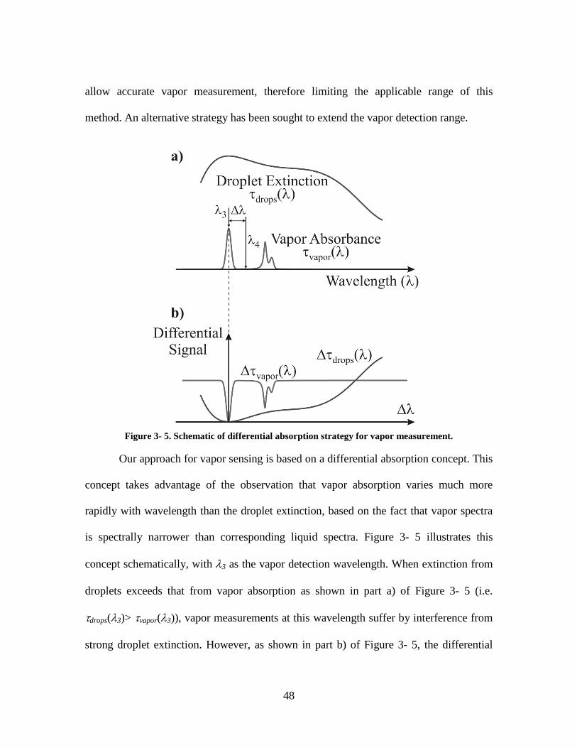
48
allow accurate vapor measurement, therefore limiting the applicable range of this
method. An alternative strategy has been sought to extend the vapor detection range.
Figure 3- 5. Schematic of differential absorption strategy for vapor measurement.
Our approach for vapor sensing is based on a differential absorption concept. This
concept takes advantage of the observation that vapor absorption varies much more
rapidly with wavelength than the droplet extinction, based on the fact that vapor spectra
is spectrally narrower than corresponding liquid spectra. Figure 3- 5 illustrates this
concept schematically, with λ3 as the vapor detection wavelength. When extinction from
droplets exceeds that from vapor absorption as shown in part a) of Figure 3- 5 (i.e.
τdrops(λ3)> τvapor(λ3)), vapor measurements at this wavelength suffer by interference from
strong droplet extinction. However, as shown in part b) of Figure 3- 5, the differential

49
vapor absorption between λ3 and another wavelength λ4 (defined as ∆τvapor = |τvapor(λ3) -
τvapor(λ4)|), can be comparable or larger than the differential droplet extinction (defined as
∆τdrops = |τdrops(λ3) - τdrops(λ4)|), therefore extending accurate vapor detection into a wider
dynamic range.
3.5.2 Selection of Wavelengths
Obviously the selection of wavelengths (λ3 and λ4) to optimize vapor detection
depends on the spectra of the specific vapor and liquid under consideration. This section
again uses water as an example to illustrate a methodology for wavelength selection, but
the approach is also applicable to other vapor and liquid systems.
We first examine the dependence of differential droplet extinction (∆τdrops) on
selected wavelengths (λ3 and λ4) with the goal of minimizing differential droplet
extinction. Substitution of Equation (3.7) (from mono-dispersed droplets) into the
definition of ∆τdrops yields
3 43 | ( , ) ( , ) | 3
2 2V V
drops
C Q D Q D L C LQ
D D
λ λτ
−∆ = = ⋅∆ (3.15)
Therefore the dependence of ∆τdrops on selected wavelengths is equivalent to the
dependence of ∆Q (i.e. the differential extinction coefficient) on selected wavelengths.
Figure 3- 6 shows the droplet extinction coefficient and vapor absorption over
wavelength in a spectral range from 0.5 to 9 µm for water vapor and droplets with two

50
diameters, using the liquid spectra data of water measured in [68, 69]; and the vapor
spectra is simulated using HITRAN 2004. Note the relative slow variation of extinction
coefficient compared to that of vapor with wavelength, as mentioned before. Examination
of ∆Q at different combinations of λ3 and λ4 within this spectral range shows a general
profile of ∆Q similar to that shown in Figure 3- 7, where λ3 is chosen to be 5 µm.
Figure 3- 6. Extinction coefficients for water droplets with different diameters and vapor absorbance
from water vapor from 0.5 to 9 µµµµm at 220C.
Figure 3- 7 reveals that multiple combinations of wavelengths can be applied to
achieve small ∆Q for a given droplet diameter. For example, for a droplet diameter of 6
µm and a λ3 of 5 µm, either a λ4 near 5 or 3 µm results in small ∆Q. These wavelength
combinations can be divided into two categories. The first category is a combination of
two wavelengths close to each other (i.e. λ3 = 5 µm and λ4 close to 5 µm in the above
example), and the second is a combination of two wavelengths well separated from each
other (i.e. λ3 = 5 µm and λ4 close to 3 µm in the above example). However, the second

51
category of wavelength combinations is only applicable to cases with small droplet size
changes. As shown in Figure 3- 7, when droplet diameter changes from 6 to 3 µm, ∆Q
increases by a large amount if λ4 is well separated from λ3, while small ∆Q is maintained
if λ4 is close to λ3. Mathematical considerations of the dependence of Q on droplet size
and wavelength validate the generalization of above observations. Therefore, in general,
wavelengths for vapor measurement by differential absorption must be close to each
other for applications with varying droplet size.
Figure 3- 7. ∆∆∆∆Q for water droplet with different diameters when λλλλ3 is selected at 5 µµµµm.
Next, we consider the dependence of differential vapor absorption (∆τvapor) on
selected wavelengths (λ3 and λ4) with the goal of maximizing differential vapor
absorption. Apparently, maximum differential absorption is achieved by selecting one
wavelength (e.g. λ3) where the strongest vapor absorption occurs and another wavelength
(e.g. λ4) where the weakest vapor absorption occurs over the entire spectral range of

52
interest. For the example of water as shown in Figure 3- 6, one wavelength (λ3) can be at
a vapor absorption peak near 2.7 or 5.9 µm. Part a) of Figure 3- 8 shows the selection of
λ3 at 2.6705 µm, where maximum vapor absorbance occurs in the 2.5 to 3.0 µm spectral
range. For the case with varying droplet size, which is of major interest to this work, the
second wavelength (λ4) must be close to λ3. Part b) of Figure 3- 8 shows water vapor
spectra in the vicinity of 2.6705 µm. In principle, a λ4 chosen to be as close to λ3 as
possible provided that vapor does not absorb at this wavelength can minimize ∆τdrops
while maintaining maximum ∆τvapor. A λ4 of 2.6720 µm as shown in part b) of Figure 3-
8 is an example of such a choice. But in practice, other considerations such as avoiding
interference from pressure broadening of the vapor spectra, may encourage a different
selection of λ4, for example, 2.6818 µm as shown.
Figure 3- 8. Wavelength selection of differential absorption scheme for water with a temperature of
220C, total pressure 1 atm, mole fraction of water vapor 3%, and pathlength of 1cm.
Finally, we evaluate the applicable range of the above differential scheme for
water vapor detection in an evaporating spray. Here we consider a system of water
aerosols bathed in an inert gas undergoing uniform evaporation at constant pressure (1

53
atm) and temperature (220C), as a simplified model of the aerosol evaporation behind
shock waves [64]. The system starts at time=0 with all droplets at diameter D0, droplet
volume fraction CV0, and no vapor. As time progresses, the diameter of the droplets (D)
and the droplet volume fraction (CV) decreases due to evaporation and, consequently, the
mole fraction of water vapor in the system increases. The differential scheme designed
above with λ3 at 2.6705 and λ4 at 2.6818 µm is applied to monitor vapor concentration.
Comparison between ∆τdrops and ∆τvapor during the evaporation process provides an
evaluation of the applicable range of this vapor sensing scheme in terms of droplet size
(D), droplet loading (CV), and mole fraction of vapor. This work uses the range where
∆τvapor exceeds ∆τdrops to quantify the applicable range of the differential absorption
scheme.
This comparison is complicated because it depends on both initial droplet
diameter (D0) and droplet volume fraction (CV0). Comparison at some representative
initial diameter is therefore used to provide an insight into the applicable range of the
differential absorption scheme. One such representative diameter can be obtained by
seeking a diameter to maximize differential droplet extinction (∆τdrops) in Equation (3.18)
for a given combination of differential absorption wavelengths. This initial diameter,
denoted as max0D , results in maximum ∆τdrops at time=0 in the evaporation process.
Furthermore, both mathematical considerations and numerical computations reveal that
other initial diameters will yield similar or smaller ∆τdrops during the entire evaporation
process compared to that yielded atmax0D . Therefore, comparison between ∆τdrops and

54
∆τvapor at max0D provides a lower limit of the applicable range of the differential
absorption, i.e. the applicable range for other initial droplet diameters will be similar or
wider than that evaluated at max0D . For the differential scheme shown in Figure 3- 8 (λ3 at
2.6705 and λ4 at 2.6818 µm), max0D is found to be 5.1 µm. Therefore, the range where
∆τvapor exceeds ∆τdrops evaluated at max0D =5.1 µm represents a lower limit of the
applicable range of this differential absorption scheme, and this scheme can be applied
for vapor detection in a wider range at other D0’s .
Figure 3- 9. Comparison of droplet extinction and vapor absorption at a wavelength of λλλλ3=2.6705 µµµµm
for the evaporation process depicted in Figure 3- 10 to evaluate the applicable range of single wavelength scheme for vapor detection. Evaluation performed at a temperature of 220C, pressure 1
atm, and pathlength of 1 cm.
Vapor absorption and droplet extinction at a single wavelength (λ3=2.6705 µm)
are first calculated in Figure 3- 9 for a few initial droplet volume fractions at D0=5.1 µm.
Note a CV0 of 19.36 ppm (parts per million) corresponds to the case that the saturated

55
water vapor pressure at the given temperature is reached when all the droplets in the
system are evaporated. Therefore, at a CV0 higher than 19.36 ppm (for example 40 ppm),
the saturated water vapor pressure is reached when the droplets are only partially
evaporated (about 50% evaporated in the example of CV0=40 ppm), and vapor absorption
becomes a constant afterwards. Figure 3- 9 suggests that accurate vapor measurement by
single wavelength is jeopardized by large droplet extinction interference for some range
of droplet volume fraction while vapor absorption itself is strong enough to allow
accurate vapor measurement. For example, for the case when CV0=40 ppm, after about
10% of the droplets are evaporated, the vapor absorbance reaches about 10% and
accurate vapor detection can be readily performed at this absorbance level. However,
droplet extinction imposes significant interference on vapor detection because τdrops
exceeds τvapor by almost a factor of three at this stage of evaporation as shown in Figure
3- 9. Once at least 22% of the droplet volume evaporates (i.e. CV/CV0<78%), τvapor starts
to exceed τdrops, and this single wavelength detection scheme becomes applicable
afterwards by the definition in this work.
The differential absorption strategy extends the vapor measurement into the range
where strong interference from droplet extinction impairs the utility of single wavelength
detection. Figure 3- 10 shows the comparison between ∆τdrops and ∆τvapor when the
differential scheme (λ3 at 2.6705 and λ4 at 2.6820 µm) is applied to the evaporating
process described above. Obviously, ∆τvapor starts to exceed ∆τdrops much earlier in the
process than τvapor starts to exceed τdrops in Figure 3- 9, therefore, a wider domain of

56
accurate vapor detection is achieved using differential absorption. In the case shown in
Figure 3- 10, vapor detection is limited by the magnitude of vapor absorption itself, not
by interference from droplet extinction as in the case of Figure 3- 9. For example, for the
case when CV0=40 ppm, after about 2% of the droplets are evaporated (i.e. CV/CV0<98%),
vapor absorbance starts to exceed droplet extinction and, therefore, the differential
absorption scheme becomes applicable for vapor detection afterward. Although
differential vapor absorbance is low (~1.5%) because the vapor concentration is low at
this stage of evaporation, stronger differential signal can be achieved by utilizing a longer
pathlength. Note that a D0 of 3.0 µm results in smaller ∆τdrops than that from a D0 of 5.1
µm, as expected. Also note that the applicable range of differential absorption is not
strongly sensitive to normalized droplet volume fraction (i.e. CV/CV0) from Figure 3- 10.
Figure 3- 10. Comparison of differential droplet extinction and vapor absorption between the
wavelengths chosen in Figure 3- 9 for the evaporation process depicted in Figure 3- 10 to evaluate the applicable range of the differential absorption scheme for vapor detection. Evaluation performed at
a temperature of 220C, pressure 1 atm, and pathlength of 1 cm.
57
3.5.3 Differential Absorption and Wavelength Availability
Discussions in Section 3.5.2 are based on the assumption that light sources are
available at any wavelength to allow the utilization of the strongest differential vapor
absorption. Although the strongest differential vapor absorption cannot be always
accessed in practice due to the lack of light sources at proper wavelengths, it can be
shown that differential absorption always extends vapor detection into wider domain
compared with the single wavelength technique. Major conclusions about wavelength
selection are transferable to other droplet/vapor systems than water and the methodology
demonstrated above can be used evaluate the applicable range of specific differential
absorption scheme. For example, currently there are no convenient and economical laser
devices to provide the wavelengths near 2.67 µm shown in Figure 3- 8, but diode laser
sources are readily available to access the absorption spectra by water vapor near 1.39
µm, where the strongest absorption of the υ1+υ3 band of water vapor occurs. Though the
absorption from water vapor near 1.39 µm is weaker than that near 2.67 µm by about an
order of magnitude, a differential absorption scheme based on the absorption features
near 1.39 µm still enables ∆τvapor to start to exceed ∆τdrops in an early stage of evaporation
in the process described above and, therefore, allows accurate vapor detection in a wide
range of droplet loading and vapor concentration.

58
3.6 Summary
Design criteria and methods are developed for selecting the optimum wavelengths
for simultaneous droplet size and vapor concentration in sprays. These criteria and
methods are applied to the design of a sensor for water aerosols and water vapor
measurements. The expected performance of the sensor is simulated for an evaporating
spray containing both droplet and vapor to support application for temporally-resolved
measurements. These results demonstrated that the new sensing technique significantly
extends the applicable range of extinction and absorption methods, in terms of the range
of the droplet size, number density of the droplets, and concentration of the vapor. This
work provides a systematical summary of the theory for simultaneously measuring
droplet/vapor based on laser extinction, and is expected to lay the groundwork for
implementing optical sensors based on WMLE in a variety of research and industrial
applications involving multi-phase flows.
3.7 Acknowledgement
Part of this research was conducted under the advisory of Professor Ronald K.
Hanson at Stanford University. I want to thank Professor Hanson for his guidance and
support during the course of this work.
59
Chapter 4: Investigation of Temperature
Parallel Simulated Annealing for
Optimizing Continuous Functions with
Application to Hyperspectral
Tomography
4.1 Abstract
The simulated annealing (SA) algorithm is a well-established optimization
technique which has found applications in many research areas. However, the SA
algorithm is limited in its application due to the high computational cost and the
difficulties in determining the annealing schedule. This paper demonstrates that the
temperature parallel simulated annealing (TPSA) algorithm, a parallel implementation of
the SA algorithm, shows great promise to overcome these limitations when applied to
continuous functions. The TPSA algorithm greatly reduces the computational time due
to its parallel nature, and avoids the determination of the annealing schedule by fixing the
temperatures during the annealing process. The main contributions of this paper are

60
threefold. First, this paper explains a simple and effective way to determine the
temperatures by applying the concept of critical temperature (TC). Second, this paper
presents systematic tests of the TPSA algorithm on various continuous functions,
demonstrating comparable performance as well-established sequential SA algorithms.
Third, this paper demonstrates the application of the TPSA algorithm on a difficult
practical inverse problem, namely the hyperspectral tomography problem. The results
and conclusions presented in this work provide are expected to be useful for the further
development and expanded applications of the TPSA algorithm.
4.2 Introduction
The simulated annealing (SA) algorithm was first introduced in 1983 for solving
combinatorial optimization problems [15]. Since then, it has been extensively studied,
with successful demonstrations of its use for both discrete [16, 17] and continuous
optimization problems [18-23]. These past research efforts have shown several critical
advantages of the SA algorithm over other optimization techniques. For example, it can
optimize complicated problems with a large number of variables and numerous confusing
local minima. In addition, the SA algorithm is insensitive to the initial guess, which is
especially important when no a priori information about the solutions is available.
On the other hand, the disadvantages of the SA algorithm are also well-
recognized. One of the primary disadvantages of the SA algorithm is its high
computational cost [20, 23]. Many research efforts that have focused on developing
variants of the SA algorithm to reduce the computational cost [24-26] can be divided into
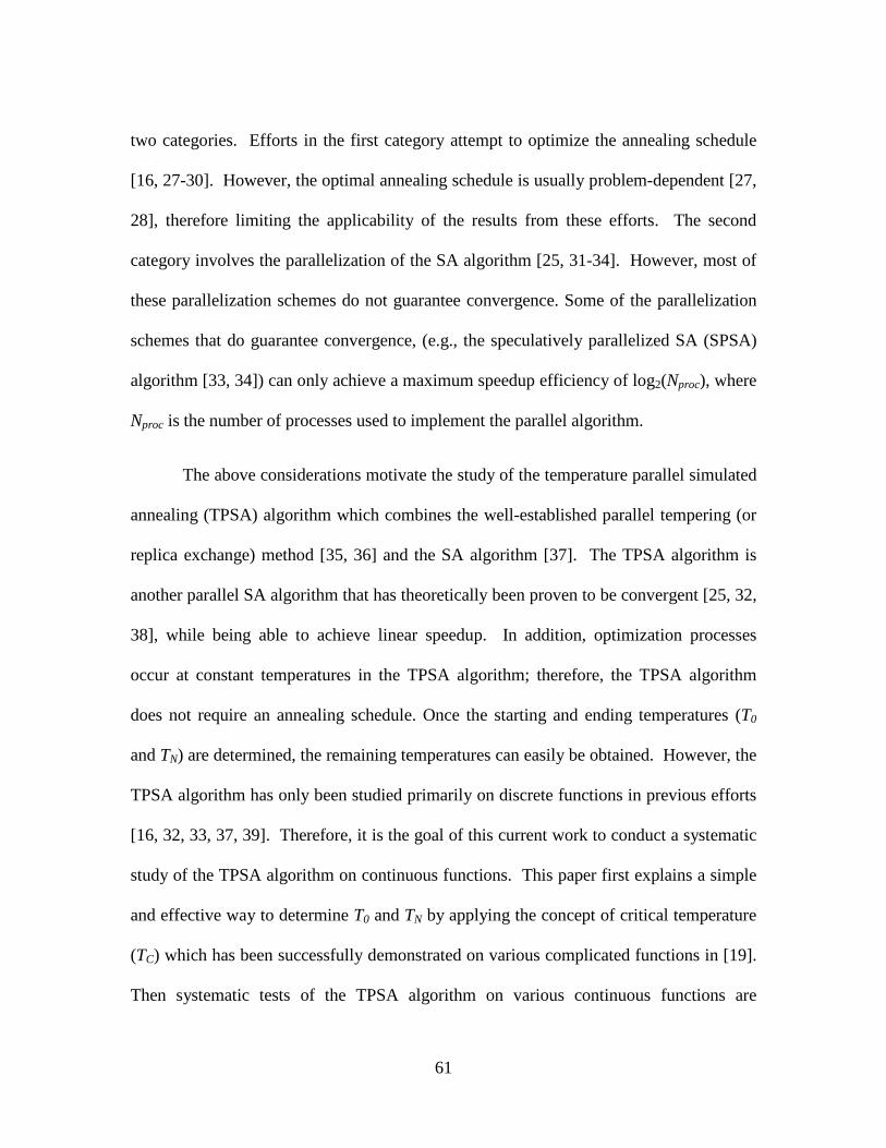
61
two categories. Efforts in the first category attempt to optimize the annealing schedule
[16, 27-30]. However, the optimal annealing schedule is usually problem-dependent [27,
28], therefore limiting the applicability of the results from these efforts. The second
category involves the parallelization of the SA algorithm [25, 31-34]. However, most of
these parallelization schemes do not guarantee convergence. Some of the parallelization
schemes that do guarantee convergence, (e.g., the speculatively parallelized SA (SPSA)
algorithm [33, 34]) can only achieve a maximum speedup efficiency of log2(Nproc), where
Nproc is the number of processes used to implement the parallel algorithm.
The above considerations motivate the study of the temperature parallel simulated
annealing (TPSA) algorithm which combines the well-established parallel tempering (or
replica exchange) method [35, 36] and the SA algorithm [37]. The TPSA algorithm is
another parallel SA algorithm that has theoretically been proven to be convergent [25, 32,
38], while being able to achieve linear speedup. In addition, optimization processes
occur at constant temperatures in the TPSA algorithm; therefore, the TPSA algorithm
does not require an annealing schedule. Once the starting and ending temperatures (T0
and TN) are determined, the remaining temperatures can easily be obtained. However, the
TPSA algorithm has only been studied primarily on discrete functions in previous efforts
[16, 32, 33, 37, 39]. Therefore, it is the goal of this current work to conduct a systematic
study of the TPSA algorithm on continuous functions. This paper first explains a simple
and effective way to determine T0 and TN by applying the concept of critical temperature
(TC) which has been successfully demonstrated on various complicated functions in [19].
Then systematic tests of the TPSA algorithm on various continuous functions are

62
reported, demonstrating comparable performance as well-established sequential SA
algorithms.
The above studies are directly motivated by a practical application, in which a so-
called hyperspectral tomography problem is desired to be solved efficiently to obtain in
situ measurements of the temperature and concentration of chemical species [8, 9].
Therefore, the application of the TPSA algorithm developed in this paper was also
applied to solve the hyperspectral problem, illustrating its usefulness and potential for
practical applications.
The remainder of this paper is organized as follows. Section 4.3 provides a
detailed introduction to the TPSA algorithm. Section 4.4 discusses the determination of
the T0 and TN using the concept of TC, while Sections 4.5 and 4.6 evaluate the
performance of the TPSA algorithm in terms of accuracy and computational time.
Section 4.7 discusses the impact of other parameters important to the TPSA algorithm,
including the relationship between the speedup efficiency and the number of processes
(Nproc), and the effects of the exchange frequency (EF). Section 4.8 describes the
application of the TPSA algorithm to a practical problem, where the TPSA algorithm was
applied to perform tomographic inversion of hyperspectral measurements. Finally,
Section 4.9 summarizes the paper.

63
4.3 Temperature Parallel Simulated Annealing
The TPSA algorithm, a parallel implementation of the SA algorithm, offers two
advantages over sequential SA algorithms: 1) the determination of the annealing schedule
can be avoided by fixing the temperatures as constant throughout the optimization
process, and 2) a reduction in computational time can be achieved. Note that under the
context of the SA algorithm, the term “temperature” represents a parameter used in the
algorithm, to be differentiated from the physical temperature to be measured in the
hyperspectral tomography technique later in Section 4.8 of the paper.
The mechanism of the TPSA algorithm has been explained elsewhere under the
context of combinatorial optimization [16, 32], and is illustrated in Figure 4- 1 and briefly
summarized here. First, N+1 temperatures (T0 to TN) are generated and dispatched to
N+1 processes. Then, each process performs an optimization procedure using a
sequential SA algorithm with the assigned temperature fixed as constant. Here, a well-
established sequential SA algorithm described in [20] is used. After a pre-set number of
iterations on each process, the processes with adjacent temperatures (labeled as T and T’
in Figure 4- 1) exchange their optimal solutions as shown in Figure 4- 1. The exchange
occurs at a probability p as defined in Figure 4- 1. If the solution at the higher
temperature exhibits a smaller function value than that of the lower temperature, the
solutions are always exchanged. Otherwise, the solutions will be exchanged with a
probability less than 1. The specific value of the probability is determined by the

64
temperature difference between T and T’ (labeled as ∆T) and the difference in the
functional values (labeled as ∆f).
Figure 4- 1. Illustration of the TPSA algorithm.
This procedure of exchanging solutions starts from the processes with the two
highest temperatures and proceed to those with the two lowest temperatures. Therefore,
the downward direction of the exchange tends to concentrate the solutions with smaller
function values at lower temperatures, where further reduction in function values is more
likely to occur and to converge. However, meanwhile, it also becomes less likely to
escape local minima at lower temperatures. This issue is solved by the upward direction
of the exchange, where the local minima at lower temperatures can be transferred to
higher temperatures, allowing the TPSA algorithm to escape the local minima and find
the global minimum.
One important parameter involved in the above procedure is the frequency of the
exchange, EF. This paper defines the EF as follows:

65
1adjstep
EFN
= (4.1)
where adjstepN is the number of the step-length adjustments before each solution exchange.
See [20] for more details about the adjustment of the step-length in the sequential SA.
This paper defines the following quantity, ∆F, to quantify the performance of
optimization:
globalF F F∆ = − (4.2)
where F is the minimum value of the target function obtained, and Fglobal the global
minimum of the target function. Obviously, a ∆F of zero means the algorithm has found
the global minimum; and a smaller ∆F means the algorithm has approached a solution
that is closer to the global minimum.
Figure 4- 2. Evolution of ∆F for both the SSA and TPSA algorithms.
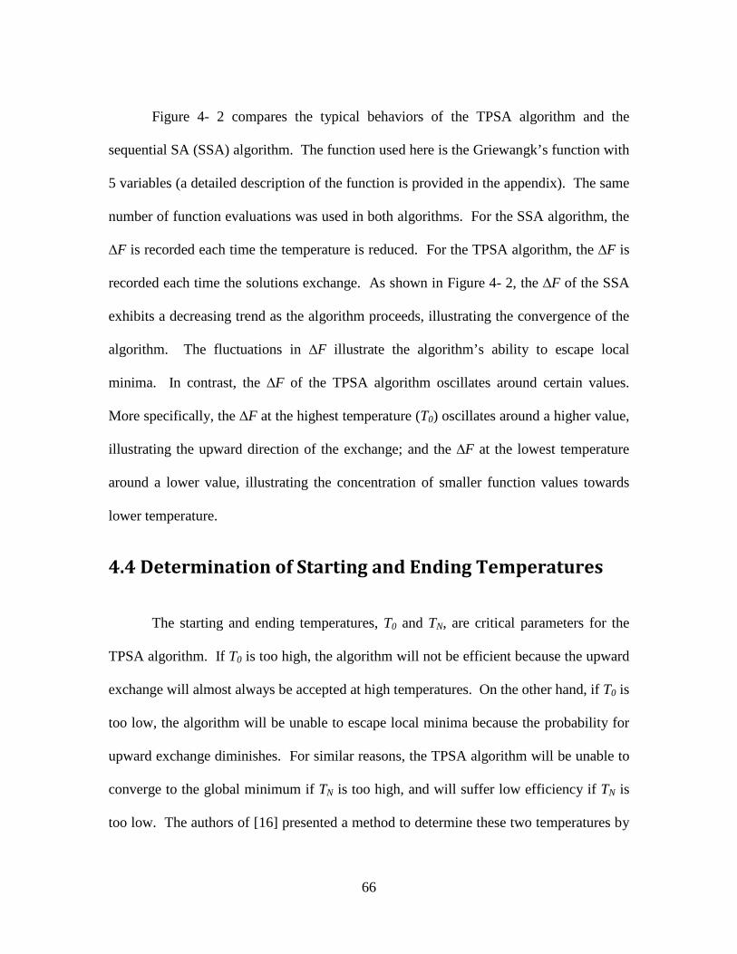
66
Figure 4- 2 compares the typical behaviors of the TPSA algorithm and the
sequential SA (SSA) algorithm. The function used here is the Griewangk’s function with
5 variables (a detailed description of the function is provided in the appendix). The same
number of function evaluations was used in both algorithms. For the SSA algorithm, the
∆F is recorded each time the temperature is reduced. For the TPSA algorithm, the ∆F is
recorded each time the solutions exchange. As shown in Figure 4- 2, the ∆F of the SSA
exhibits a decreasing trend as the algorithm proceeds, illustrating the convergence of the
algorithm. The fluctuations in ∆F illustrate the algorithm’s ability to escape local
minima. In contrast, the ∆F of the TPSA algorithm oscillates around certain values.
More specifically, the ∆F at the highest temperature (T0) oscillates around a higher value,
illustrating the upward direction of the exchange; and the ∆F at the lowest temperature
around a lower value, illustrating the concentration of smaller function values towards
lower temperature.
4.4 Determination of Starting and Ending Temperatures
The starting and ending temperatures, T0 and TN, are critical parameters for the
TPSA algorithm. If T0 is too high, the algorithm will not be efficient because the upward
exchange will almost always be accepted at high temperatures. On the other hand, if T0 is
too low, the algorithm will be unable to escape local minima because the probability for
upward exchange diminishes. For similar reasons, the TPSA algorithm will be unable to
converge to the global minimum if TN is too high, and will suffer low efficiency if TN is
too low. The authors of [16] presented a method to determine these two temperatures by

67
utilizing the Genetic Algorithm (GA). The authors tested their method on combinatorial
problems [16] and observed encouraging results. However, it has been noted that
incorporating the GA further complicates the optimization algorithm by requiring
elaborate parameter tuning [75]. Other authors suggested adaptive T0 and TN by
maintaining empirically determined acceptance ratio [76], which also complicates the
implementation of the algorithm. This work, therefore, seeks an alternative simple
approach to determine the T0 and TN.
Figure 4- 3. Determination of T0 and TN using the TC-curve.

68
The critical temperature, TC, is an important and useful concept in the SA
algorithm. It has been found that the SA algorithm explores the searching space more
efficiently at TC than at other temperatures [27, 29, 30]. A recent work has examined the
application of TC in minimizing continuous functions using sequential SA algorithms
[19]. Here, we found that the use of TC is also effective in determining the starting and
ending temperatures for the TPSA algorithm. As to be discussed in Sections 4.5 and 4.6,
using the starting and ending temperatures determined by TC, the TPSA algorithm
provides comparable performance to well established SSA algorithms.
Figure 4- 3 illustrates the concept of TC, using the Schewefel’s function with 4
variables, which is denoted as fS4. A detailed description of this function and the method
to generate the results shown here can be found in [19]. Briefly, the SSA algorithm was
conducted independently at 10 constant temperatures ranging from ~10-5 to ~106. At
each temperature, 10 cases were performed and the mean value and standard deviation
(std) of the ∆F’s were recorded. The top panel of Figure 4- 3 shows the mean value of
the ∆F’s with the error bar representing the std of the ∆F’s, while the bottom panel shows
the std. The results shown in Figure 4- 3 clearly illustrate that the SA algorithm exhibits
three distinct behaviors at different temperature regions. First, when the temperature is
high (>105), the output from the algorithm is characterized by a large ∆F and std. The
reason for this behavior is that when the temperature is sufficiently high, the SA
algorithm essentially samples the function randomly, resulting in high ∆F and std.
Second, when the temperature is sufficiently low (<100), the algorithm essentially
samples the local minima of the function randomly because the algorithm cannot escape a

69
local minimum once the algorithm enters one, resulting in high ∆F and std again. Third,
in the temperature range of ~ 102 to 104, the results are characterized by both small ∆F
and std. This paper names the temperature at which the smallest std of ∆F’s occurs as TC
(TC~103 for the fS4 function), and the curve shown in the lower panel of Figure 4- 3 the
TC-curve. It has been shown that, in the region near TC, the SA algorithm has a high
probability of locating the global minimum for various problems with complicated
energy landscapes as demonstrated in [19].
Here, we use the TC-curve generated as described above to determine the starting and
ending temperatures for the TPSA algorithms. Specifically, the starting and ending
temperatures are chosen to be the temperature immediately higher and lower than TC,
respectively, as shown on the TC-curve. The effectiveness of this simple scheme will be
demonstrated in Sections 4.5 and 4.6.
4.5 Evaluation of Performance
To evaluate the performance of the TPSA algorithm and the effectiveness of the
scheme for determining T0 and TN, a TPSA algorithm was implemented in FORTRAN 90
and compared to a well-established SSA algorithm [20]. Note that there are also other
variations of the SSA algorithms [10, 11], and it would be interesting to examine which
SSA algorithm is optimal for parallelizing under the TPSA scheme. However, such an
examination is out of the scope of this current work, and merits a full-length paper by
itself. Therefore, in this work, we chose to work with a well established SSA algorithm

70
[6]. In the SSA, a relative change of function values (εSA=10-6) during two consecutive
temperature reductions was used as the termination criterion. Two measures were taken
to make the results comparable. First, both algorithms are performed using the same
number of function evaluations. More specifically, the SSA algorithm was run using the
parameters recommended in [20] and the aforementioned stop criteria of εSA=10-6 was
implemented. Upon the termination of the SSA algorithm, the number of evaluations of
the target function was recorded. Then the same number of function evaluations was
assigned evenly across all the processes used in the TPSA algorithm. The TPSA
algorithm was terminated when the number of function evaluations at each process
reached its assigned quota. Second, a local search was performed at the end of the SSA
and TPSA algorithms. The local search guarantees that the global minimum will be
found if either algorithm can locate a solution near the global minimum. The local search
used the quasi-Newton method with the termination criterion set as εLocal=10-8, where
εLocal is the relative change of function values between two consecutive function
evaluations. The computational cost of the local search was less than 1% of SA
evaluations in both the SSA and TPSA algorithms.
The comparisons were made on various functions, each representing a unique
optimization challenge. For example, the Michalewicz's function with 10 variables (fM10)
has a global minimum hidden in a deep narrow valley buried among 10! (~3.6×10⁶) local
minima, and the Schwefel's function (fS8) function has a global minimum far from the
local minima. More details about these test functions can be found in the appendix of
[19] and also in the appendix of this paper.

71
Number of Function
Evaluations SSA
TPSA TPSA TPSA
(EF=1)
(EF=6.25×10⁻²)
(EF=3.91×10⁻³)
fB2 1.60 X 10⁴ 1.00 X 10⁻¹⁶ 1.00 X 10⁻¹⁶ 1.00 X 10⁻¹⁶ 1.00 X 10⁻¹⁶
fG5 1.25 X 10⁶ 2.91 X 10⁻¹⁴ 1.00 X 10⁻¹⁶ 1.00 X 10⁻¹⁶ 9.86 X 10⁻³
fM2 2.00 X 10⁵ 2.60 X 10⁻¹³ 5.11 X 10⁻¹⁴ 3.76 X 10⁻¹³ 4.22 X 10⁻¹³
fM5 1.00 X 10⁶ 2.70 X 10⁻¹¹ 4.36 X 10⁻¹² 4.76 X 10⁻¹² 4.73 X 10⁻¹²
fM10 2.00 X 10⁶ 1.14 X 10⁻¹³ 2.74 X 10⁻¹¹ 2.74 X 10⁻¹¹ 1.45 X 10⁻¹¹
fRa1
0 2.50 X 10⁶ 6.48 X 10⁻¹² 1.00 X 10⁻¹⁶ 8.88 X 10⁻¹⁵ 9.95 X 10⁻¹
fRo5 1.10 X 10⁶ 1.69 X 10⁻¹¹ 2.67 X 10⁻¹⁰ 3.13 X 10⁻¹¹ 1.18 X 10⁻¹⁰
fS4 1.00 X 10⁶ 7.40 X 10⁻³ 5.51 X 10⁻¹² 5.29 X 10⁻¹² 5.51 X 10⁻¹²
fS8 1.20 X 10⁶ 2.98 X 100 1.07 X 10⁻¹¹ 1.01 X 10⁻¹¹ 1.08 X 10⁻¹¹
fS12 2.32 X 10⁶ 8.11 X 10⁻¹¹ 1.61 X 10⁻¹¹ 1.68 X 10⁻¹¹ 1.73 X 10⁻¹¹
Table 4- 1. The best ∆F of SSA and TPSA on the Selected Test Functions
To compare the SSA and TPSA algorithms, a TC-curve was generated for each of
the test functions, from which the T0 and TN for the TPSA algorithm and the initial
temperature for the SSA algorithm were determined. All computations were performed
on two Dell workstations with dual Intel Xeon quad-core processors (X5482, 3.2 GHz).
A set of results is listed in Table 4- 1 and Table 4- 2, and plotted in Figure 4- 4. The
results are presented in terms of ∆F as defined before and also in terms of ∆x as defined
below to quantify the distance between the solution obtained and the true solution at the
global minimum:

72
globalx x x∆ = − (4.3)
where x is the solution obtained from the SSA or TPSA algorithm, and xglobal is the
solution at the global minimum. For each function, 30 runs were performed using either
the SSA or TPSA algorithm, with different random seeds. The best results from these 30
runs were selected and listed in Table 4- 1 and Table 4- 2, and also plotted in Figure 4- 4
for better visualization. The results from the TPSA algorithm are reported at three
different EF’s to illustrate the effects of exchange frequency.
Number of Function
Evaluations SSA
TPSA TPSA TPSA
(EF=1) (EF=6.25×10⁻²) (EF=3.91×10⁻³)
fB2 1.60 X 10⁴ 3.06 X 10⁻¹⁰ 9.20 X 10⁻¹⁰ 4.35 X 10⁻¹⁰ 7.54 X 10⁻¹⁰
fG5 1.25 X 10⁶ 3.41 X 10⁻⁸ 2.93 X 10⁻⁹ 1.69 X 10⁻⁹ 6.28 X 100
fM2 2.00 X 10⁵ 6.55 X 10⁻⁸ 4.53 X 10⁻⁸ 6.17 X 10⁻⁸ 5.75 X 10⁻⁸
fM5 1.00 X 10⁶ 2.43 X 10⁻⁷ 9.91 X 10⁻⁸ 1.63 X 10⁻⁷ 1.50 X 10⁻⁷
fM10 2.00 X 10⁶ 1.86 X 10⁻⁶ 2.63 X 10⁻⁷ 2.63 X 10⁻⁷ 2.42 X 10⁻⁷
fRa10 2.50 X 10⁶ 7.43 X 10⁻⁶ 1.20 X 10⁻¹⁰ 7.19 X 10⁻¹¹ 9.95 X 10⁻¹
fRo5 1.10 X 10⁶ 1.18 X 10⁻⁵ 2.51 X 10⁻⁵ 8.87 X 10⁻⁶ 2.01 X 10⁻⁵
fS4 1.00 X 10⁶ 5.44 X 100 7.16 X 10⁻⁷ 3.45 X 10⁻⁶ 3.94 X 10⁻⁶
fS8 1.20 X 10⁶ 1.72 X 100 1.61 X 10⁻⁶ 1.54 X 10⁻⁶ 3.04 X 10⁻⁶
fS12 2.32 X 10⁶ 4.82 X 10⁻⁷ 4.19 X 10⁻⁶ 8.20 X 10⁻⁶ 1.00 X 10⁻⁵
Table 4- 2. The best ∆x of SSA and TPSA on the Selected Test Functions
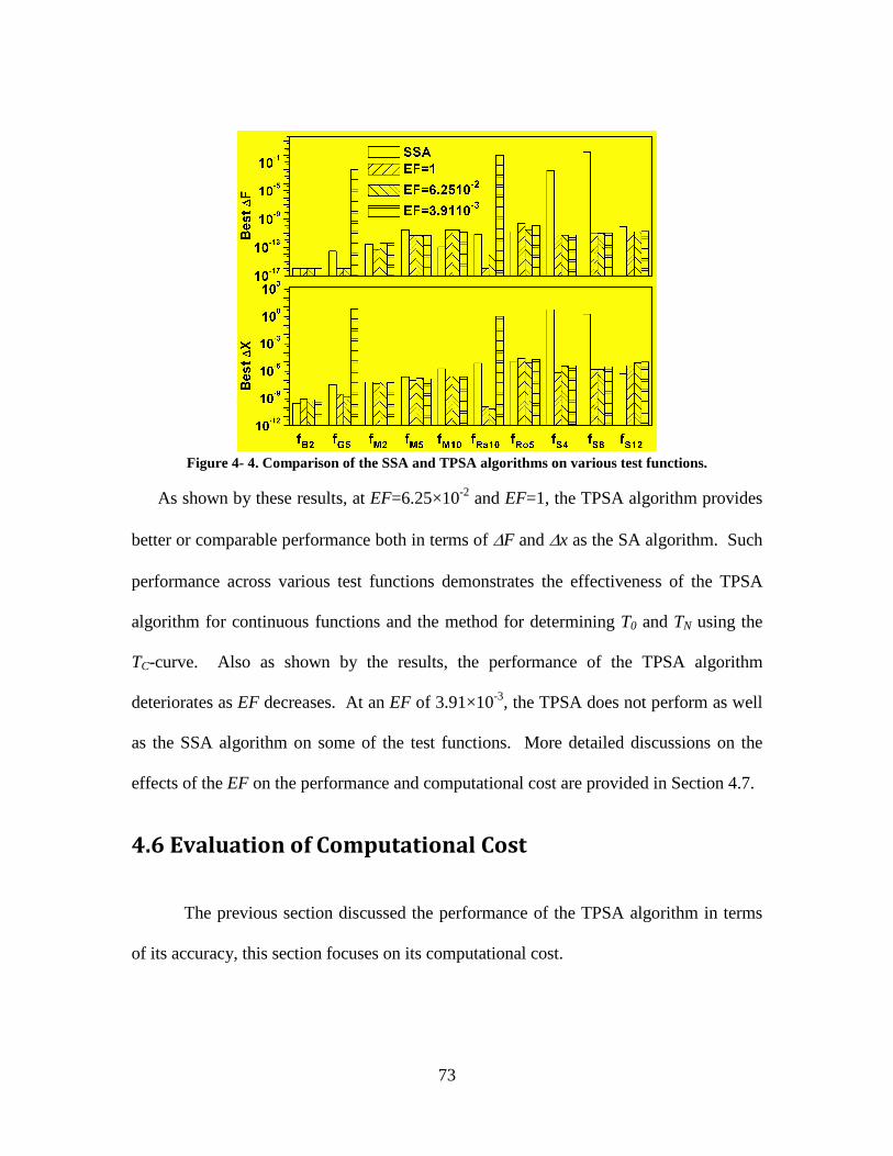
73
Figure 4- 4. Comparison of the SSA and TPSA algorithms on various test functions.
As shown by these results, at EF=6.25×10⁻² and EF=1, the TPSA algorithm provides
better or comparable performance both in terms of ∆F and ∆x as the SA algorithm. Such
performance across various test functions demonstrates the effectiveness of the TPSA
algorithm for continuous functions and the method for determining T0 and TN using the
TC-curve. Also as shown by the results, the performance of the TPSA algorithm
deteriorates as EF decreases. At an EF of 3.91×10⁻³, the TPSA does not perform as well
as the SSA algorithm on some of the test functions. More detailed discussions on the
effects of the EF on the performance and computational cost are provided in Section 4.7.
4.6 Evaluation of Computational Cost
The previous section discussed the performance of the TPSA algorithm in terms
of its accuracy, this section focuses on its computational cost.

74
Figure 4- 5. Computational time of the TPSA algorithm as a function of the exchange frequency.
First, the effects of EF on the computational cost were examined. Figure 4- 5
illustrates the impact of the EF on the computational time of the TPSA algorithm. The
TPSA algorithms at various EF’s ranging from ~10-2 to 1 are implemented using 16
processes and applied to 3 test functions, and the actual computational time (the wall-
clock time) was recorded and plotted in Figure 4- 5. The same number of functions
evaluations was (as determined by the method described at the beginning of Section 4.5)
performed at each EF for each test function. As illustrated by these results, the
computational time increases as EF increases, due to the computational overhead
involved in evaluating the exchange criteria and in exchanging information between
different processes. At an EF=1, the actual computational time was about 3× more than
that at an EF=6.25×10⁻²; and the benefits of such increased computational time were the
improved performance as shown in Table 4- 1 and Table 4- 2. These computational
times were also compared with the time when EF was set to zero. When EF=0, the

75
TPSA algorithm essentially reduces to a series of classic Metropolis algorithms, each
running at a fixed temperature. The computational time in this case represents the time
for actually evaluating the functions (i.e., without evaluating the exchange criterion and
without communication between the processes). These times were shown on Figure 4- 5
by the straight lines labeled EF=0. The difference between the computational times at
various EF’s and that at EF=0 represents the computational overhead in the TPSA
algorithm due to exchanges.
Second, the effects of the number of processes (Nproc) on the computational cost
were examined. Ideally, the computational time should exhibit a linear or super-linear
dependence on Nproc. Here, to quantify the speedup efficiency of the TPSA algorithm,
the following parameter (Φ) is defined:
Computational time of SSA
(Computational time of TPSA) procNΦ =
⋅ (4.4)
where all the times are wall-clock time. Clearly, Φ indicates the efficiency of the parallel
algorithm: Φ=1 means a linear speedup, Φ>1 a super-linear speedup, and Φ<1 stands for
a sub-linear speedup. Figure 4- 6 shows the relationship between Φ and Nproc at different
EF’s for two test functions. The TPSA algorithm was implemented on various numbers
of processes ranging from 2 to 64. At each Nproc, 30 test runs were conducted. The points
in the figure represent the mean value of Φ for these 30 cases and the error bars the std.
As Figure 4- 6 shows, the std is generally quite small (too small to be visible in many
cases shown here), evidencing the repeatability of the runs.
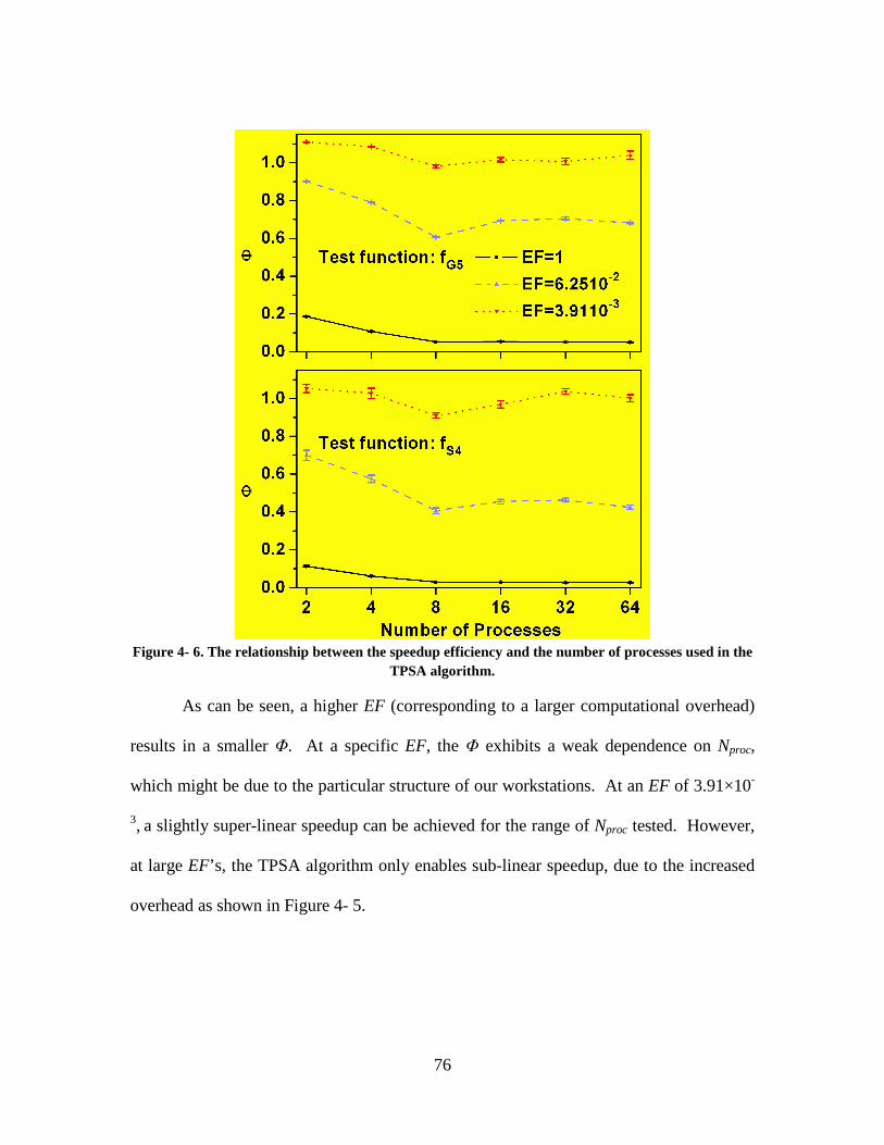
76
Figure 4- 6. The relationship between the speedup efficiency and the number of processes used in the
TPSA algorithm.
As can be seen, a higher EF (corresponding to a larger computational overhead)
results in a smaller Φ. At a specific EF, the Φ exhibits a weak dependence on Nproc,
which might be due to the particular structure of our workstations. At an EF of 3.91×10-
3, a slightly super-linear speedup can be achieved for the range of Nproc tested. However,
at large EF’s, the TPSA algorithm only enables sub-linear speedup, due to the increased
overhead as shown in Figure 4- 5.

77
4.7 Preliminary Study of Exchange Frequency
The results reported in Sections 4.5 and 4.6 suggest that TPSA provides better
performance at larger EF, at the cost of increased computational time. Therefore, it is
highly desirable to have some insight into optimizing the tradeoff between the
performance and computational time. Previous studies on such optimization have
focused on discrete functions [16, 32], and have shown that the performance of the TPSA
algorithm becomes insensitive to EF after a certain value. Here, we examined the
dependence of the TPSA’s performance on EF for continuous functions, and found that
the pattern of the dependence is more complicated than for discrete functions.
Two representative patterns were selected and shown in Figure 4- 7 and Figure 4-
8. In these figures, the TPSA algorithm was implemented on 16 processes to minimize
various test functions, and 30 cases were run on each test function. The mean and std
(represented by the error bar) of the ∆F obtained for these 30 cases were shown here.
Figure 4- 7 shows the “normal” patterns, i.e., the performance of the TPSA improves as
EF increases for the test functions shown in Figure 4- 7. This pattern is what one would
intuitively expect: the algorithm should locate the global minimum more accurately if
information across at different processes is exchanged more frequently. In contrast, the
patterns shown in Figure 4- 8 are “abnormal”, where the performance shows a weak or
even fluctuating dependence on EF. As the top panel of Figure 4- 8 shows, for the fS4
function, the performance (again measured in terms of ∆F and its std) fluctuates with EF;
and the bottom panel of Figure 4- 8 shows a weak dependence for the fRo5 function.

78
Figure 4- 7. Impact of the exchange frequency on the performance of the TPSA algorithm for the
fRa10 and fS12 functions.
Though the dependence of TPSA’s performance on EF is complicated as
discussed above and remains as on ongoing research direction, several preliminary
observations can be made for optimizing the tradeoff between performance and
computational cost. First, an EF larger than 6.25×10⁻² already provided comparable
performance to the SSA algorithm as shown in Table 4- 1 and Table 4- 2, and in Figure
4- 4. Also, TPSA’s performance at an EF of 6.25×10⁻² is only worse than at an EF of 1
marginally. Second, as Figure 4- 5 shows, the computational time at EF=1 is about 3×

79
more than that at EF~10-3 due to the increased computational overhead. Such overhead
will decrease (relative to the computational time for evaluating the target function) when
the target function becomes more expensive to evaluate, and many target functions in
practice are considerably more expensive to evaluate than the test functions used here.
Therefore, using an EF=1 might be a feasible practical strategy for many applications.
Our results agree with the conclusion of [77], which also suggests low exchange
frequency.
Figure 4- 8. Impact of the exchange frequency on the performance of the TPSA algorithm for the fS4
and fRo5 functions.

80
4.8 Application to Hyperspectral Tomography
This section describes the application of the TPSA developed above in a so-called
hyperspectral tomography (HT) problem. The goal of the HT problem is to image the
distribution of the property of a chemical species (e..g, temperature or concentration)
using of line-of-sight-integrated absorption measurements at various wavelengths. The
HT problem is highly nonlinear and computationally intensive [4, 8, 9]. Thus there is a
strong motivation to parallelize the solution of the HT problem, so that it can be solved
quickly for in situ analysis.
Figure 4- 9. The mathematical formulation of the hyperspectral tomography problem.
The mathematical background and experimental demonstration of the HT
problem has been detailed in [4, 8] and [9], respectively. A brief summary is provided
here for convenience. The configuration of the HT problem is illustrated in Figure 4- 9.
A hyperspectral laser beam (i.e., a laser beam that scans a wide wavelength range) is
directed along the line of sight, denoted by l, to probe the domain of interest as shown in
the left. Absorption by the target species will attenuate the probe laser beam, and the
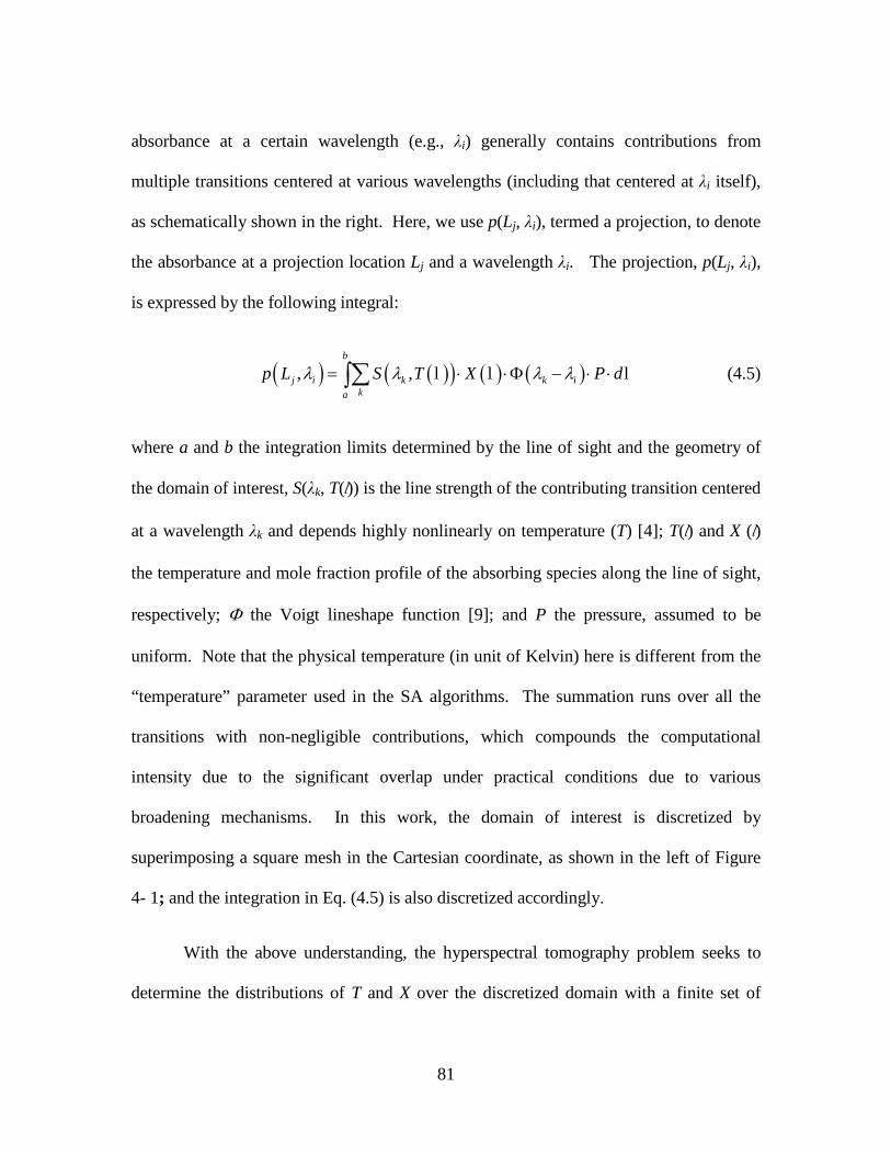
81
absorbance at a certain wavelength (e.g., λi) generally contains contributions from
multiple transitions centered at various wavelengths (including that centered at λi itself),
as schematically shown in the right. Here, we use p(Lj, λi), termed a projection, to denote
the absorbance at a projection location Lj and a wavelength λi. The projection, p(Lj, λi),
is expressed by the following integral:
( ) ( )( ) ( ) ( ), ,b
j i k k ika
p L S T X P dλ λ λ λ= ⋅ ⋅Φ − ⋅ ⋅∑∫ l l l (4.5)
where a and b the integration limits determined by the line of sight and the geometry of
the domain of interest, S(λk, T(l)) is the line strength of the contributing transition centered
at a wavelength λk and depends highly nonlinearly on temperature (T) [4]; T(l) and X (l)
the temperature and mole fraction profile of the absorbing species along the line of sight,
respectively; Φ the Voigt lineshape function [9]; and P the pressure, assumed to be
uniform. Note that the physical temperature (in unit of Kelvin) here is different from the
“temperature” parameter used in the SA algorithms. The summation runs over all the
transitions with non-negligible contributions, which compounds the computational
intensity due to the significant overlap under practical conditions due to various
broadening mechanisms. In this work, the domain of interest is discretized by
superimposing a square mesh in the Cartesian coordinate, as shown in the left of Figure
4- 1; and the integration in Eq. (4.5) is also discretized accordingly.
With the above understanding, the hyperspectral tomography problem seeks to
determine the distributions of T and X over the discretized domain with a finite set of
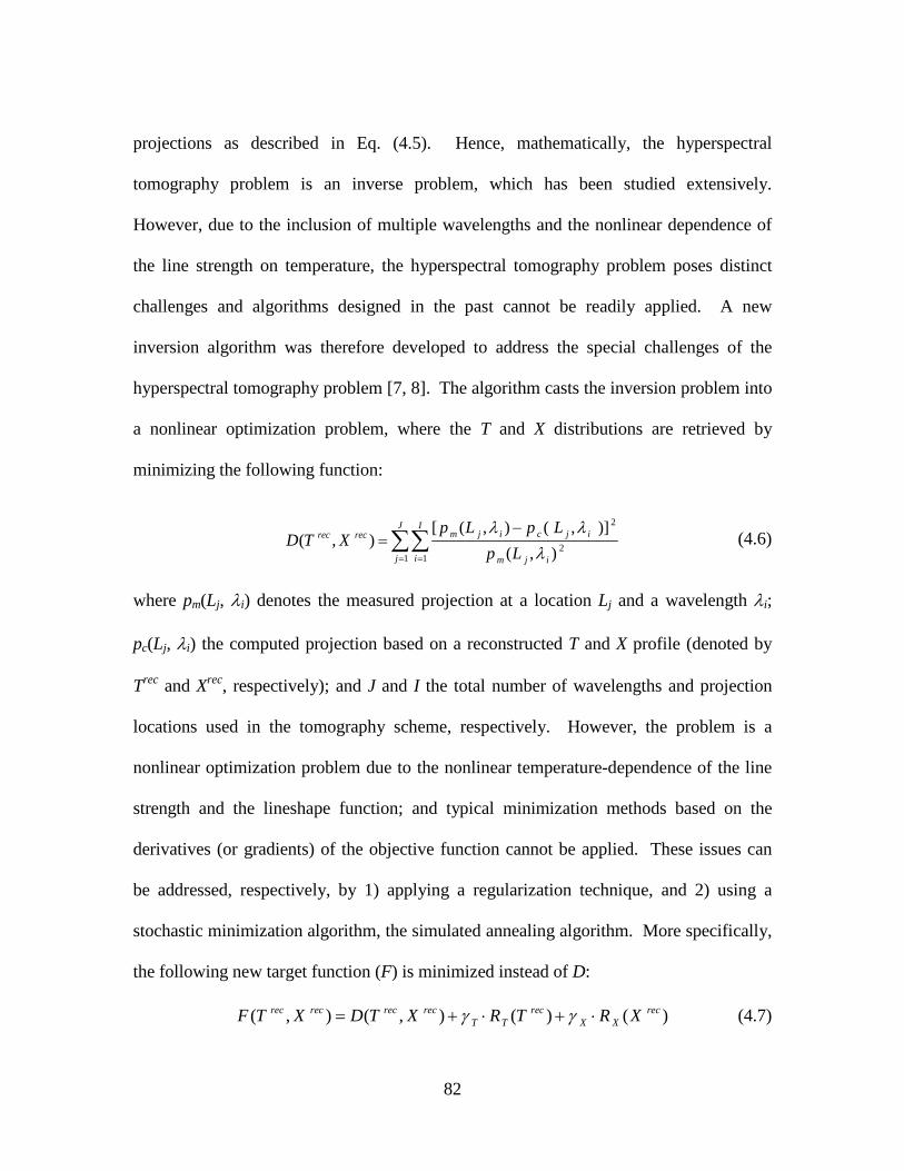
82
projections as described in Eq. (4.5). Hence, mathematically, the hyperspectral
tomography problem is an inverse problem, which has been studied extensively.
However, due to the inclusion of multiple wavelengths and the nonlinear dependence of
the line strength on temperature, the hyperspectral tomography problem poses distinct
challenges and algorithms designed in the past cannot be readily applied. A new
inversion algorithm was therefore developed to address the special challenges of the
hyperspectral tomography problem [7, 8]. The algorithm casts the inversion problem into
a nonlinear optimization problem, where the T and X distributions are retrieved by
minimizing the following function:
2
21 1
[ ( , ) ( , )]( , )
( , )
J Im j i c j irec rec
j i m j i
p L p LD T X
p L
λ λ
λ= =
−= ∑∑
(4.6)
where pm(Lj, λi) denotes the measured projection at a location Lj and a wavelength λi;
pc(Lj, λi) the computed projection based on a reconstructed T and X profile (denoted by
Trec and Xrec, respectively); and J and I the total number of wavelengths and projection
locations used in the tomography scheme, respectively. However, the problem is a
nonlinear optimization problem due to the nonlinear temperature-dependence of the line
strength and the lineshape function; and typical minimization methods based on the
derivatives (or gradients) of the objective function cannot be applied. These issues can
be addressed, respectively, by 1) applying a regularization technique, and 2) using a
stochastic minimization algorithm, the simulated annealing algorithm. More specifically,
the following new target function (F) is minimized instead of D:
( , ) ( , ) ( ) ( )rec rec rec rec rec recT T X XF T X D T X R T R Xγ γ= + ⋅ + ⋅ (4.7)

83
where RT and RX are the regularization factors for temperature and concentration,
respectively; γT and γX are positive constants (regularization parameters) to scale the
magnitude of RT and RX properly such that they do not dominate the D(Trec, Xrec) term.
The master function, F, is then minimized using the simulated annealing algorithm; and
finally, the solution of the minimization problem described in Eq. (4.7) provides the
tomographic reconstruction of the T and X distributions.
Figure 4- 10. Comparison of T phantom and reconstruction obtained using the TPSA algorithm.
Here, we applied the TPSA algorithm to the HT problem, demonstrating its
comparable performance to previous techniques at reduced computational time. The left
panel of Figure 4- 10 shows an example T phantom used in the study. The phantoms
were generated over a 10-by-10 square grid by superimposing two Gaussian peaks on a
paraboloid to simulate a representative multi-modal and asymmetric temperature
distribution of H2O in practical combustion devices. Other distribution phantoms have
been tested and the results obtained are similar to those obtained with the phantoms
shown here. A hypothetical HT sensor with 20 beams is applied to probe the
distributions, with 10 beams probing in the horizontal direction and the other 10 in the
vertical direction. Each beam contains 10 wavelengths, probing 10 different transitions of

84
H2O. A set of simulated projections was then generated according to Eq. (4.5), and the
TPSA algorithm was applied to solve the HT problem by minimizing Eq, (4.7). A
reconstructed T distribution is shown in the mid panel, and the difference between the
reconstruction and the phantom shown in the right panel. The inversion was performed
on the Dell workstation with two Intel Xeon quad-core processors (X5482, 3.2 GHz) and
eight processes was applied in the TPSA algorithm. We chose to conduct this study on
such a workstation instead of on a large number of processors because the primary object
is to examine whether it is feasible to process hyperspectral tomography data in situ on a
small workstation or a PC. According to our computational experiments, the HT problem
depends weakly on EF and the EF used here was chosen to be 0.125, considering the fact
that the computation of the target function in Eq. (4.7) is considerably more costly than
the exchange overhead. As these results show, the TPSA algorithm yielded
reconstructions with high fidelity. In the example results shown here, the reconstruction
error was within -40 K to 60 K and the overall reconstruction error was 1.56% (defined
as error relative to the phantom averaged over all grids).
In comparison, Fig. 11 shows an example reconstruction using the sequential SSA
algorithm [8]. The left panel shows the reconstruction, the mid panel shows the
difference relative to the phantom, and the right panel shows the difference relative to the
results obtained by the TPSA algorithm shown in Fig. 10. The overall reconstruction
error was 1.59% in this case. The results in Fig. 10 and Fig. 11 demonstrated that the
TPSA algorithm can achieve comparable reconstruction fidelity as the SSA algorithm.

85
Figure 4- 11. Reconstruction obtained using the SSA algorithm in comparison to the phantom and
that obtained using the TPSA algorithm.
Solving this example problem using the sequential SA algorithm required 430
seconds (~ 7 minutes) of computation time, and 102 seconds (~ 1.7 minutes) using the
TPSA algorithm, representing around 4× reduction in computational time. The
computation costs approximately scales linearly with the number of grids (i.e., a 20×20
case will require 4× more computation time than the 10×10 case). A 10×10 case
represents a typical current hyperspectral tomography application because of two
considerations. First, a 10×10 discretization is already sufficient for many practical
applications; and second, a finer discretization poses implementation difficulty in practice
in terms of optical access, laser power availability, etc. The processing time also varies
approximately linearly with the number of wavelengths used, and the specific
configuration of the workstation. A 1.7-minute processing time in our current study
shows good promising of the TPSA for in situ analysis of HT measurements in many
practical applications.

86
4.9 Summary
To summarize, this paper provides a systematic investigation of the TPSA
algorithm on continuous functions, with application to a practical problem where
tomographic reconstruction of a chemical species is obtained using hyperspectral
absorption measurements. Two aspects of the algorithm were considered. First, this
work developed a simple and effective way to determine the starting and ending
temperatures for TPSA using the critical temperature. Second, this work conducted an
extensive comparison of the TPSA algorithm against a well-established sequential SA
algorithm, and demonstrated that comparable performance can be achieved. The results
show that the TPSA algorithm is a reliable method which can achieve comparable
performance to the SSA algorithm while greatly reducing the computational time.
Implications of these findings are discussed under the context of the hyperspectral
tomography problem. This work is expected to lay the groundwork for further
development of the TPSA algorithm, and for its expanded applications.
4.10 Acknowledgements
Special thanks are due to Barbara Ramirez for her assistance in preparing the
manuscript.
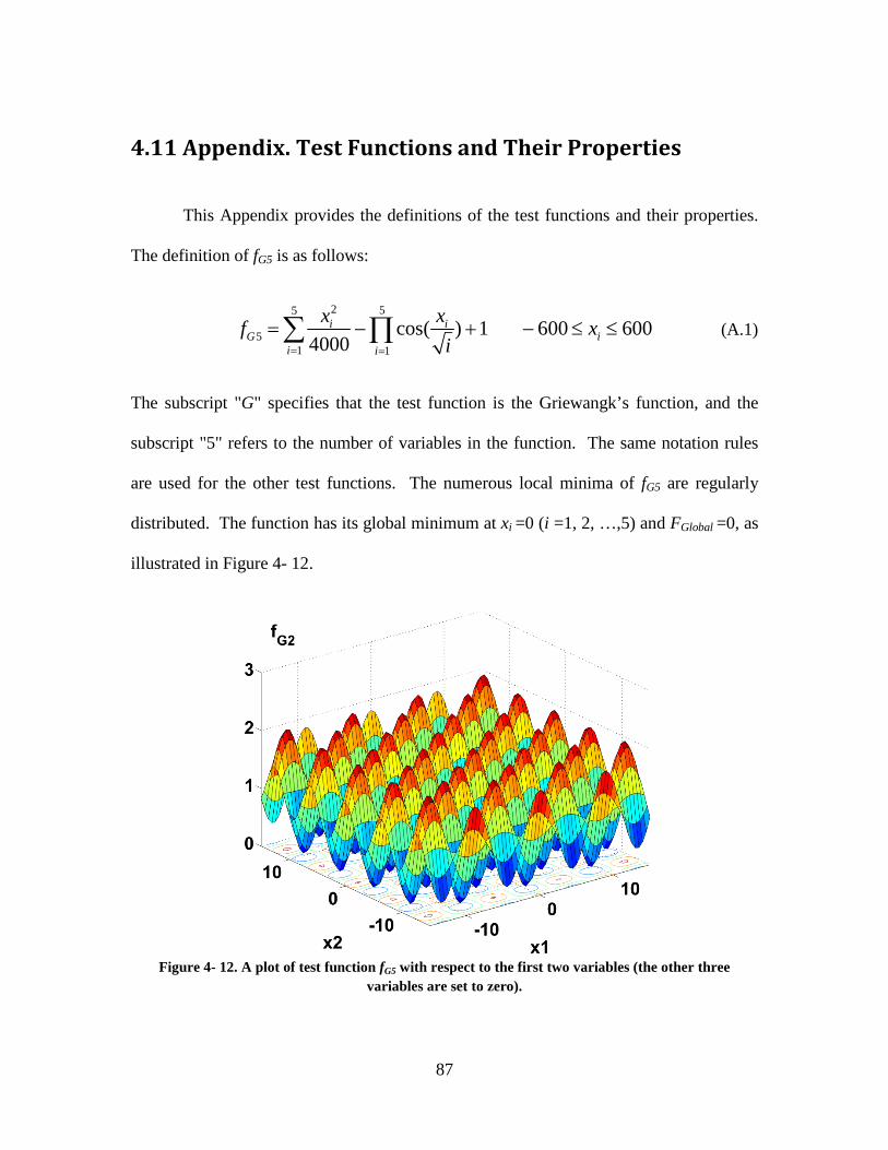
87
4.11 Appendix. Test Functions and Their Properties
This Appendix provides the definitions of the test functions and their properties.
The definition of fG5 is as follows:
2 55
51 1
cos( ) 1 600 6004000
i iG i
i i
x xf x
i= =
= − + − ≤ ≤∑ ∏ (A.1)
The subscript "G" specifies that the test function is the Griewangk’s function, and the
subscript "5" refers to the number of variables in the function. The same notation rules
are used for the other test functions. The numerous local minima of fG5 are regularly
distributed. The function has its global minimum at xi =0 (i =1, 2, …,5) and FGlobal =0, as
illustrated in Figure 4- 12.
Figure 4- 12. A plot of test function fG5 with respect to the first two variables (the other three
variables are set to zero).

88
The definition of fRa10 is as follows:
10
210
1
100 ( 10 cos(2 )) 5.12 5.12Ra i i ii
f x x xπ=
= + − ⋅ ⋅ ⋅ − ≤ ≤∑ (A.2)
The function has its global minimum at xi =0 (i =1, 2, …, 10) and FGlobal =0. This
function shares similar features with fG5, whose local minima are regularly distributed, as
illustrated in Figure 4- 13.
Figure 4- 13. A plot of test function fRa10 with respect to the first two variables (the other variables
are set to zero).
The next function, fB2, is defined as:
2 22 1 2 1 2 1 22 0.3cos(3 ) 0.4cos(4 ) 0.7 -1 , 1Bf x x x x x xπ π= + − − + ≤ ≤ (A.3)
The global minimum of fB2 is at (0, 0) and FGlobal =0. Figure 4- 14 shows a plot of test
function fB2, illustrating the many irregularly distributed local minima.

89
Figure 4- 14. A plot of test function fB2.
The Michalewicz’s function with n variables is defined as:
2
2
1
sin [sin( )] 0n
miMn i i
i
i xf x x π
π=
⋅= − ≤ ≤∑ (A.4)
This function has a global minimum hidden in a deep narrow valley buried among n!
local minima. The parameter m defines the sharpness of the valley containing the global
minimum. Figure 4- 15 shows an example of the Michalewicz’s function with five
variables (n=5) with the first three variables set to zero), illustrating the large number of
local minima and the steepness of the global minimum.

90
Figure 4- 15. A plot of test function fM5 with respect to the fourth and fifth variables (the first three variables are set to zero).
The Schwefel’s function with n variables is defined as:
1
sin 500 500n
Sn i i ii
f x x x=
= − ⋅ − ≤ ≤∑ (A.5)
This function has its global minimum at xi =420.9687 (i =1, 2, …, n) and FGlobal =-
418.9829·n. This function is characterized by a large number of local minima, which are
widely separated from each other, as illustrated by the plot in Figure 4- 16 shows (n=2).
Figure 4- 16. A plot of the fS2 test function.

91
The last test function is the Rosenbrock’s function (also known as the Banana
function) with 5 variables. The Rosenbrock’s function with n variables is defined as:
1
2 2 21
1
100 ( ) (1 ) 2.048 2.048n
Ron i i i ii
f x x x x−
+=
= ⋅ − + − − ≤ ≤∑ (A.6)
This function features a global minimum that is hidden inside a long and twisted flat
valley. Finding the valley is trivial, however, navigating through the valley and locating
the exact location of the global minimum is challenging. This function has a global
minimum at xi =1 (i =1, 2, …, 5) and FGlobal =0. Figure 4- 17 shows a plot of the function
with two variables, illustrating the shape and flatness of the valley, inside which the
global minimum is located.
Figure 4- 17. A plot of the fR5 test function with respect to its first two variables (other variables are set to zero).
92
Chapter 5: Conclusion
In this final chapter, the results from this work are summarized from the studies of
the application of PCMs, the development of a measurement technique for particles in
multiphase environments, and the application of the TPSA algorithm to the data analysis.
The latter two developments are expected to increase the understanding of the influence
that nanoparticle sizing has on the thermal enhancements of nanofluids.
This work first investigated the practical application of selected phase change
materials (PCMs) to a practical thermal management system for a LED headlight
assembly. The major challenge was the fact that these organic PCMs, while possessing
favorable latent heat properties, possessed very low thermal conductivities that would
render any practical application of these materials not feasible. However, with the
emergence of metal foams which can suspend these PCMs, the effective thermal
conductivity can be increased to a level that is practical in a thermal management system.
It is very clear that, for the system studied, PCMs show great promise in protecting the
LED headlight system. PCMs provide delayed time to reach the failure temperature of
these components and are easily integrated into this system without requiring additional
energy input. Finally, an optimization process found the optimal volume fraction of the
PCM that maximizes the operational time of the LED headlight assembly. These results
should not only prove the applicability of using PCMs to protect the studied LED

93
headlight system, but also demonstrate the applicability of using PCMs in many other
systems needing enhanced thermal protection.
Next, in order to enhance the favorable characteristics of the PCM based thermal
management system, this work investigated methods to measure the size of nanoparticles
within a nanofluid in order to understand the effect that sizing has on the nanofluid. This
study focused on developing a method to be applied to the multiphase flow problem of
detecting the size of particles within a multiphase environment. The expected
performance of the sensor is simulated.
Finally, this work endeavored to improve the inversion algorithm of the data by
increasing the fidelity of solution while decreasing the computational time, which should
prove valuable to the study of nanofluids. This work developed a new method based on
simulated annealing for analyzing the data in a parallelized fashion (TPSA). By
conducting an extensive comparison of the TPSA algorithm against a well-established
sequential simulated annealing (SSA) algorithm, this work demonstrated that comparable
performance can be achieved with reduced computation time. The results showed that
the TPSA algorithm is a reliable method which can achieve comparable performance to
the SSA algorithm while greatly reducing the computational time. Results of the TPSA
algorithm given by this work are expected to lay the groundwork for further development
of the detection of nanoparticles sizing characteristics in a nanofluid.

94
References
1. A. Pasupathy, R. Velraj, and R. V. Seeniraj, "Phase change material-based building architecture for thermal management in residential and commercial establishments," Renewable & Sustainable Energy Reviews 12, 39-64 (2008).
2. M. M. Farid, A. M. Khudhair, S. A. K. Razack, and S. Al-Hallaj, "A review on phase change energy storage: materials and applications," Energy Conversion and Management 45, 1597-1615 (2004).
3. D. L. Vrable, and K. L. Yerkes, "A thermal management concept for more electric aircraft power system applications," SAE Technical Paper Series 981289, 1-6 (1998).
4. S. A. Khateeb, M. M. Farid, J. R. Selman, and S. Al-Hallaj, "Design and simulation of a lithium-ion battery with a phase change material thermal management system for an electric scooter," Journal of Power Sources 128, 292-307 (2004).
5. R. Kandasamy, X. Q. Wang, and A. S. Mujumdar, "Transient cooling of electronics using phase change material (PCM)-based heat sinks," Applied Thermal Engineering 28, 1047-1057 (2008).
6. P. Gauche, and X. Weiran, "Modeling phase change material in electronics using CFD - a case study," in 2000 International Conference on High-Density Interconnect and Systems Packaging, 402-407 (2000).
7. S. Krishnan, and S. V. Garimella, "Analysis of a phase change energy storage system for pulsed power dissipation," IEEE Transactions on Components and Packaging Technologies 27, 191-199 (2004).
8. S. Krishnan, J. Y. Murthy, and S. V. Garimella, "Analysis of solid-liquid phase change under pulsed heating," Journal of Heat Transfer-Transactions of the ASME 129, 395-400 (2007).
9. D. W. Yoo, and Y. K. Joshi, "Energy efficient thermal management of electronic components using solid-liquid phase change materials," IEEE Transactions on Device and Materials Reliability 4, 641-649 (2004).
10. T. Aldoss, D. J. Ewing, Y. Zhao, and L. Ma, "Numerical investigation of phase change materials for thermal management systems," SAE Technical Paper Series, (2009).

95
11. A. S. Fleischer, R. D. Weinstein, and T. Kopec, "Analysis of transient thermal management characteristics of PCM with an embedded carbon heat sink," in The Tenth Intersociety Conference on Thermal and Thermomechanical Phenomena in Electronics Systems, (2006), pp. 1265-1268.
12. S. T. Hong, and D. R. Herling, "Open-cell aluminum foams filled with phase change materials as compact heat sinks," Scripta Materialia 55, 887-890 (2006).
13. P. A. E. Vallejos, and C. Duston, "Carbon foam filled with phase change materials for passive temperature management," in COMSOL Multiphysics Users (2005).
14. V. V. Kulish, and J. L. Lage, "Diffusion within a porous medium with randomly distributed heat sinks," International Journal of Heat and Mass Transfer 43, 3481-3496 (2000).
15. S. Kirkpatrick, C. D. Gelatt Jr, and M. P. Vecchi, "Optimization by simulated annealing," Science 220, 671-680 (1983).
16. M. Miki, T. Hiroyasu, J. Wako, and T. Yoshida, "Adaptive temperature schedule determined by genetic algorithm for parallel simulated annealing," in The 2003 Congress Evolutionary Computation, 459-466 (2003).
17. E. L. Piccolomini, and F. Zama, "The conjugate gradient regularization method in computed tomography problems," Applied Mathematics and Computation 102, 87-99 (1999).
18. W. Cai, D. J. Ewing, and L. Ma, "Application of simulated annealing for multispectral tomography," Computer Physics Communications 179, 250-255 (2008).
19. W. Cai, and L. Ma, "Applications of critical temperature in minimizing functions of continuous variables with simulated annealing algorithm," Computer Physics Communications 181, 11-16 (2010).
20. A. Corana, M. Marchesi, C. Martini, and S. Ridella, "Minimizing multimodal functions of continuous variables with the “simulated annealing” algorithm," ACM Transactions on Mathematical Software (TOMS) 13, 262-280 (1987).
21. L. Ma, and W. Cai, "Numerical investigation of hyperspectral tomography for simultaneous temperature and concentration imaging," Applied Optics 47, 3751-3759 (2008).
22. L. Ma, W. Cai, A. W. Caswell, T. Kraetschmer, S. T. Sanders, S. Roy, and J. R. Gord, "Tomographic imaging of temperature and chemical species based on hyperspectral absorption spectroscopy," Optics Express 17, 8602-8613 (2009).

96
23. W. H. Press, B. P. Flannery, S. A. Teukolsky, and W. T. Vetterling, Numerical Recipes (Cambridge University Press, 2007).
24. L. Ingber, "Very fast simulated re-annealing," Mathematical and Computer Modelling 12, 967-973 (1989).
25. S. W. Mahfoud, and D. E. Goldberg, "Parallel recombinative simulated annealing: A genetic algorithm," Parallel Computing 21, 1-28 (1995).
26. I. G. Tsoulos, and I. E. Lagaris, "Genanneal: Genetically modified simulated annealing," Computer Physics Communications 174, 846-851 (2006).
27. A. Basu, and L. N. Frazer, "Rapid determination of the critical temperature in simulated annealing inversion," Science 249, 1409-1412 (1990).
28. W. Ben-Ameur, "Computing the initial temperature of simulated annealing," Computational Optimization and Applications 29, 369-385 (2004).
29. H. Cohn, and M. Fielding, "Simulated annealing: Searching for an optimal temperature schedule," SIAM Journal on Optimization 9, 779-802 (1999).
30. M. Fielding, "Simulated annealing with an optimal fixed temperature," SIAM Journal on Optimization 11, 289-307 (2000).
31. J. P. B. Leite, and B. H. V. Topping, "Parallel simulated annealing for structural optimization," Computers & Structures 73, 545-564 (1999).
32. M. Miki, T. Hiroyasu, M. Kasai, K. Ono, and T. Jitta, "Temperature parallel simulated annealing with adaptive neighborhood for continuous optimization problem," International Journal of Computational Intelligence and Applications, 149-154 (2002).
33. A. Sohn, "Parallel n-ary speculative computation of simulated annealing," IEEE Transactions on Parallel and Distributed Systems 6, 997-1005 (1995).
34. E. E. Witte, R. D. Chamberlain, and M. A. Franklin, "Parallel simulated annealing using speculative computation," IEEE Transactions on Parallel and Distributed Systems 2, 483-494 (1991).
35. C. J. Geyer, and E. A. Thompson, "Annealing Markov chain Monte Carlo with applications to ancestral inference," Journal of the American Statistical Association 90, 909-920 (1995).
36. U. H. E. Hansmann, "Effective way for determination of multicanonical weights," Physical Review E 56, 6200-6203 (1997).

97
37. Y. Li, V. A. Protopopescu, N. Arnold, X. Zhang, and A. Gorin, "Hybrid parallel tempering and simulated annealing method," Applied Mathematics and Computation 212, 216-228 (2009).
38. K. Kimura, and K. Taki, "Time-homogeneous parallel annealing algorithm," in Proceedings of the 13th IMACS World Congress on Computation and Applied Mathematics, (1991).
39. D. E. Goldberg, Genetic Algorithms in Search, Optimization, and Machine Learning (Addison-Wesley Reading, Menlo Park, 1989).
40. A. Sari, and K. Kaygusuz, "Thermal energy storage system using stearic acid as a phase change material," Solar Energy 71, 365-376 (2001).
41. K. Cho, and M. Choi, "Experimental study on the application of paraffin slurry to high density electronic package cooling," Heat and Mass Transfer 36, 29-36 (2000).
42. X. M. Fang, and Z. G. Zhang, "A novel montmorillonite-based composite phase change material and its applications in thermal storage building materials," Energy and Buildings 38, 377-380 (2006).
43. Z. L. Liu, Z. Y. Wang, and C. F. Ma, "An experimental study on the heat transfer characteristics of a heat pipe heat exchanger with latent heat storage. Part II: simultaneous charging/discharging modes," Energy Conversion and Management 47, 967-991 (2006).
44. I. O. Salyer, and A. K. Sircar, "A review of phase change materials research for thermal energy storage in heating and cooling applications at the University of Dayton from 1982 to 1996," International Journal of Global Energy Issues 9, 183-198 (1997).
45. R. Akhilesh, A. Narasimhan, and C. Balaji, "Method to improve geometry for heat transfer enhancement in PCM composite heat sinks," International Journal of Heat and Mass Transfer 48, 2759-2770 (2005).
46. R. H. Henze, and J. A. C. Humphrey, "Enhanced heat-conduction in phase-change thermal-energy storage devices," International Journal of Heat and Mass Transfer 24, 459-474 (1981).
47. V. V. Calmidi, and R. L. Mahajan, "The effective thermal conductivity of high porosity fibrous metal foams," Journal of Heat Transfer 121, 466-471 (1999).
48. Y. K. Joshi, and D. Pal, "Application of Phase Change Materials to Thermal Control of Electronic Modules: A Computational Study," in Proceedings of the International Packaging Conference 10, (1995).

98
49. M. Kaviany, Principles of Heat Transfer in Porous Media (Pringer-Verlag, 1995).
50. A. D. Brent, V. R. Voller, and K. J. Reid, "Enthalpy-porosity technique for modeling convection-diffusion phase-change - application to the melting of a pure metal," Numerical Heat Transfer 13, 297-318 (1988).
51. S. Patankar, Numerical Heat Transfer and Fluid Flow (Hemisphere, 1980).
52. K. Peippo, P. Kauranen, and P. D. Lund, "A multicomponent PCM wall optimized for passive solar heating," Energy and Buildings 17, 259-270 (1991).
53. H. Zhao, and N. Ladommatos, "Optical diagnostics for soot and temperature measurement in diesel engines," Progress in Energy and Combustion Science 24, 221-255 (1998).
54. M. C. Thurber, and R. K. Hanson, "Simultaneous imaging of temperature and mole fraction using acetone planar laser-induced fluorescence," Experiments in Fluids 30, 93-101 (2001).
55. L. Ma, S. T. Sanders, J. B. Jeffries, and R. K. Hanson, "Monitoring and control of a pulse detonation engine using a diode-laser fuel concentration and temperature sensor," Proceedings of the Combustion Institute 29, 161-166 (2003).
56. J. B. Swithenbank, J. M. Beer, D. S. Taylor, D. Abbot, and G. C. McCreath, "A laser diagnostic technique for the measurement of droplet and particle size distribution," in 14th AIAA Aerospace Sciences Meeting, (1976).
57. W. D. Bachalo, and M. J. Houser, "Phase/doppler spray analyzer for simultaneous measurements of drop size and velocity distributions," Optical Engineering 23, 583-590 (1984).
58. R. A. Dobbins, and G. S. Jizmagia, "Optical scattering cross sections for polydispersions of dielectric spheres," Journal of the Optical Society of America 56, 1345-1349 (1966).
59. R. A. Dobbins, and G. S. Jizmagia, "Particle size measurements based on use of mean scattering cross sections," Journal of the Optical Society of America 56, 1351-1352 (1966).
60. L. Ma, and R. K. Hanson, "Measurement of aerosol size distribution functions by wavelength-multiplexed laser extinction," Applied Physics B-Lasers and Optics 81, 567-576 (2005).

99
61. L. A. Melton, A. M. Murray, and J. F. Verdieck, "Multiple parameter fuel spray analysis using Exciplex visualization: temperature, vapor/liquid concentrations, and oxygen pressure," in Proceedings of the Combustion Institute, (1985).
62. A. C. Chraplyvy, "Nonintrusive measurements of vapor concentrations inside sprays," Applied Optics 20, 2620-2624 (1981).
63. J. M. Tishkoff, D. C. Hammond, and A. C. Chraplyvy, "Diagnostic measurements of fuel spray dispersion," Transactions of the ASME. Journal of Fluids Engineering 104, 313-317 (1982).
64. T. C. Hanson, D. F. Davidson, and R. K. Hanson, "Shock tube measurements of water and n-dodecane droplet evaporation behind shock waves," in Proceedings of the 43rd Aerospace Sciences Meeting, AIAA-2005-0350, (2005).
65. T. C. Hanson, "The development of a facility and diagnostics for studying shock-induced behavior in micron-sized aerosols," Ph.D. Thesis, Stanford University, Stanford, CA., (2005).
66. C. F. Bohren, and D. R. Huffman, Absorption and Scattering of Light by Small Particles (Wiley-Interscience, 1983).
67. N. C. Wickramasinghe, Light Scattering Functions for Small Particles, with Applications in Astronomy (Adam Hilger, 1991).
68. G. M. Hale, and M. R. Querry, "Optical constants of water in the 200-nm to 200- mu m wavelength region," Applied Optics 12, 555-563 (1973).
69. L. Kou, D. Labrie, and P. Chylek, "Refractive indices of water and ice in the 0.65- to 2.5- µm spectral range," Applied Optics 32, 3531-3540 (1993).
70. P. C. Ariessohn, S. A. Self, and R. H. Eustis, "Two-wavelength laser transmissometer for measurements of the mean size and concentration of coal ash droplets in combustion flows," Applied Optics 19, 3775-3781 (1980).
71. N. L. Swanson, B.D. Billard, and T.L. Gennaro, "Limits of optical transmission measurements with application to particle sizing techniques," Applied Optics 38, 5887-5893 (1999).
72. K. L. Cashdollar, C. K. Lee, and J. M. Singer, "Three-wavelength light transmission technique to measure smoke particle size and concentration," Applied Optics 18, 1763-1769 (1979).
73. X. S. Cai, G. Zheng, and N. N. Wang, "A new dependent model for particle sizing with light extinction," Journal of Aerosol Science 26, 685-688 (1995).

100
74. E. Winklhofer, and A. Plimon, "Monitoring of hydrocarbon fuel-air mixtures by means of a light extinction technique in optically accessed research engines," Optical Engineering 30, 1262-1268 (1991).
75. K. Deb, and S. Agrawal, "Understanding interactions among genetic algorithm parameters," Foundations of Genetic Algorithms 5, 265-286 (1999).
76. A. Kone, and D. A. Kofke, "Selection of temperature intervals for parallel-tempering simulations," The Journal of Chemical Physics 122, 206101 (2005).
77. A. Schug, and W. Wenzel, "All-atom folding of the TRP-cage protein with an adpative parallel tempering method," Europhysics Letters 67, 307 (2004).

![phase change materials - Home - Home | BEopt Group07... · Phase Phase change Phase change materials a phase is a set of ... Phase change diagram. ... Naphthalene 80[4,11] 147.7[4,11]](https://img.pdfslide.us/doc/110x75/5aacf7167f8b9ac55c8dae8a/phase-change-materials-home-home-beopt-group07phase-phase-change-phase.jpg)