An investigation of pari-mutuel type options: the case of HuRLOs

Abstract: HuRLOs (Hurricane Risk Landfall Options) are quasi-binary options designed to hedge hur-

ricane risks in the Atlantic region of the U.S. The payoff of this option depends both on a risky event and

on the number of active options in the market, in a pari-mutuel setup similar to that of horse races. This

paper investigates strategic issues inherent to holding such options. To this end we simulate the operations

of the HuRLO market assuming rational but myopic investors. Our experiments show that the investment

strategies of players may have a significant impact on the expected utility of all players. Specifically, the

order, sequence and packaging of transactions has a non-trivial impact on the price paid and on the number

of options held by players. This makes the calculation of the "true" value of a HuRLOs, not to mention their

optimal purchase, a very complex problem. This difficulty in to calculate and purchase optimally HuRLOs

may explain the current lack of market interest for this type of insurance contract. Another reason may be

the 10 year lull in hurricanes making landfall in the United States.

JEL Classification: G22.

Keywords: Catastrophe insurance, Option pricing, Insurance and Capital market simulation, Financial

innovation, Risk sharing.

2

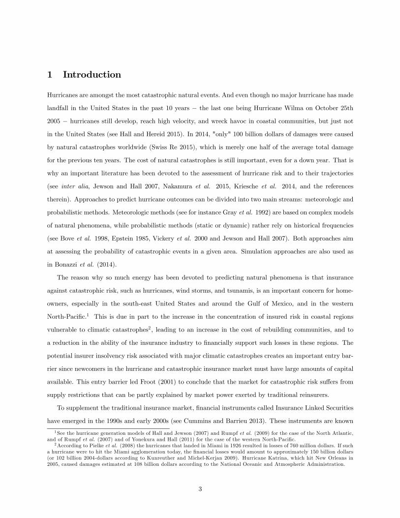
1 Introduction

Hurricanes are amongst the most catastrophic natural events. And even though no major hurricane has made

landfall in the United States in the past 10 years − the last one being Hurricane Wilma on October 25th2005 − hurricanes still develop, reach high velocity, and wreck havoc in coastal communities, but just notin the United States (see Hall and Hereid 2015). In 2014, "only" 100 billion dollars of damages were caused

by natural catastrophes worldwide (Swiss Re 2015), which is merely one half of the average total damage

for the previous ten years. The cost of natural catastrophes is still important, even for a down year. That is

why an important literature has been devoted to the assessment of hurricane risk and to their trajectories

(see inter alia, Jewson and Hall 2007, Nakamura et al. 2015, Kriesche et al. 2014, and the references

therein). Approaches to predict hurricane outcomes can be divided into two main streams: meteorologic and

probabilistic methods. Meteorologic methods (see for instance Gray et al. 1992) are based on complex models

of natural phenomena, while probabilistic methods (static or dynamic) rather rely on historical frequencies

(see Bove et al. 1998, Epstein 1985, Vickery et al. 2000 and Jewson and Hall 2007). Both approaches aim

at assessing the probability of catastrophic events in a given area. Simulation approaches are also used as

in Bonazzi et al. (2014).

The reason why so much energy has been devoted to predicting natural phenomena is that insurance

against catastrophic risk, such as hurricanes, wind storms, and tsunamis, is an important concern for home-

owners, especially in the south-east United States and around the Gulf of Mexico, and in the western

North-Pacific.1 This is due in part to the increase in the concentration of insured risk in coastal regions

vulnerable to climatic catastrophes2, leading to an increase in the cost of rebuilding communities, and to

a reduction in the ability of the insurance industry to financially support such losses in these regions. The

potential insurer insolvency risk associated with major climatic catastrophes creates an important entry bar-

rier since newcomers in the hurricane and catastrophic insurance market must have large amounts of capital

available. This entry barrier led Froot (2001) to conclude that the market for catastrophic risk suffers from

supply restrictions that can be partly explained by market power exerted by traditional reinsurers.

To supplement the traditional insurance market, financial instruments called Insurance Linked Securities

have emerged in the 1990s and early 2000s (see Cummins and Barrieu 2013). These instruments are known

1See the hurricane generation models of Hall and Jewson (2007) and Rumpf et al. (2009) for the case of the North Atlantic,

and of Rumpf et al. (2007) and of Yonekura and Hall (2011) for the case of the western North-Pacific.2According to Pielke et al. (2008) the hurricanes that landed in Miami in 1926 resulted in losses of 760 million dollars. If such

a hurricane were to hit the Miami agglomeration today, the financial losses would amount to approximately 150 billion dollars

(or 102 billion 2004-dollars according to Kunreuther and Michel-Kerjan 2009). Hurricane Katrina, which hit New Orleans in

2005, caused damages estimated at 108 billion dollars according to the National Oceanic and Atmospheric Administration.

3

as catastrophe options and catastrophe bonds, industry loss warranties, and sidecars (see Ramella and

Madeiros 2007). In contrast to traditional insurance contracts, they can be designed in a way to have very

low moral hazard and credit risk. Such interesting design features come, however, at the cost of increasing

the instruments’ basis risk (Doherty 1997). One of these new instruments is the HuRLO (Hurricane Risk

Landfall Option), launched in 2008 by Weather Risk Solutions (WRS). These options allow investors to take

positions on hurricane landfall in a similar way as in pari-mutuel3 first-by-the-post horse race betting. While

the interest in catastrophe bonds and other insurance linked securities has been growing steadily (Cummins

2008, 2012), the literature on the hurricane risk market itself is not extensive. Using data from the Hurricane

Futures Market, Kelly et al. (2012) study the traders’ perception and the trading dynamics according to

available information on hurricane risk. They conclude that relative-demand pricing is consistent with a

Bayesian update of beliefs according to information released by various official meteorological centers.

The objective of this paper is to analyze the operation of the HuRLO market by modelling the decisions

of rational risk-averse decision makers who want to hedge against catastrophic losses. Using the HuRLO as a

motivating example, Ou-Yang (2010) and Ou-Yang and Doherty (2011) compare pari-mutuel and traditional

insurance for risk-averse expected utility maximizing hedgers. They compute the optimal dynamic hedge of a

single agent in an economy where the decisions of the other players are assumed to be exogenous. Moreover,

they examine the properties of the equilibrium on that market when agents and risks are symmetrical. They

find that a pari-mutuel mechanism leads to under-insurance. They also find that pari-mutuel setting can

be advantageous when transaction costs of traditional insurance are high and when information asymmetry

problems are rampant.

With respect to HuRLOs in particular, Wilks (2010) describes their market structure, and the mecha-

nism and the adaptive algorithm used to price the options. He shows that the proposed price adjustment

mechanism converges rapidly to the market participants’ beliefs about the outcome probabilities. Meyer et

al. (2008, 2014) study the behavior of participants in an experiment of a simulated hypothetical hurricane

season, during which they are allowed to trade in both primary and secondary HuRLO markets, looking

for potential bias traditionally observed in pari-mutuel betting. They find that market prices converge to

efficient levels and that biases are not significant at the aggregate level. It therefore seems that HuRLOs

should be a perfect additional tool for hedging catastrophic loss in the Southeast United States, and in the

3The pari-mutuel mechanism was invented by Pierre Oller in 1865 in order to limit the profit of bookmarkers who were

then controlling the betting industry in France. Since 2002, many investment banks have used a pari-mutuel mechanism for

wagering on various economic statistics; odds on these statistics have been shown to be efficient forecasts of their future values

(Gürkaynak and Wolfers 2006). The pari-mutuel market microstructure is analyzed by Lange and Economides (2005) who show

the existence of a unique price equilibrium and find many advantages of pari-mutuel over the traditional exchange mechanism.

A pari-mutuel auction system for capital markets is proposed in Baron and Lange (2007).

4

state of Florida in particular.

Our contribution to the literature is two-fold: first, we examine the effectiveness of pari-mutuel insurance,

as in Ou-Yang and Doherty (2011), but in a more realistic setting, with dynamic trading, price updating,

and strategic interactions between market participants. In addition, unlike Meyer et al. (2008, 2014), our

model involves agents characterized by concave utility functions acting optimally, albeit possibly with limited

foresight.

The HuRLO market provides investors with the opportunity to hedge against, or speculate on, the risk

that a specific region in the Gulf of Mexico and on the East Coast of the U.S. will be the first to be hit by

a hurricane (or that no hurricane will make landfall in the continental United States) during a year. Many

characteristics of HuRLOs distinguish them from traditional insurance, including the fact that the payment

received neither depends on an individual’s financial loss (or lack thereof), nor on the price paid for such

protection. And because of the pari-mutuel setting, HuRLOs have characteristics that distinguish them from

standard derivatives such as: 1-the absence of counterparty and liquidity risk; 2-the absence of an underlying

traded asset; and 3-a market demand-based payoff function.

HuRLOs are interesting for both hedging and speculating purposes. On the hedging side, HuRLOs could

be useful to agents (individuals, firms or otherwise) that own assets in hurricane-prone and thus vulnerable

areas. Speculators could also participate in that market by taking advantage of differences in market-based

and objective landfall probabilities. As a competitor for traditional reinsurance products, HuRLOs have

important merits since the risk is limited to the invested capital, no counterparty is needed to assume the

position opposite to what the insurer/reinsurer desires, and there is essentially no need for a probability or

a loss appraisal since the payoff depends on market-wide factors that all but eliminate adverse selection and

moral hazard issues.

Despite such advantages and the HuRLOs’ complementarity with other forms of natural catastrophic

event hedging instruments, the market for HuRLOs has not taken off. Table 1 provides basic statistics of the

market for HuRLOs in 2009, the first (and only) year of that market’s operation where no hurricane made

landfall in the United States (thus the winning option being the "null" option). According to the Weather

Risk Solution web4 site, HuRLOs are not presently available for exchange trading.

Given the particular price formation mechanism in the HuRLO market, one interesting question is the

possible presence of strategic issues: when buying HuRLO for insurance purposes, should one place a single

order, or buy options sequentially? Should one be the first to trade, or wait to observe the trades of

4www.weatherrisksolutions.com (last visited in January 2016).

5

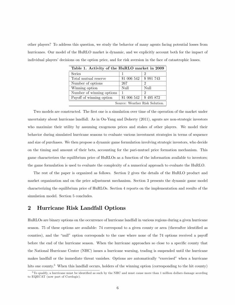
other players? To address this question, we study the behavior of many agents facing potential losses from

hurricanes. Our model of the HuRLO market is dynamic, and we explicitly account both for the impact of

individual players’ decisions on the option price, and for risk aversion in the face of catastrophic losses.

Table 1. Activity of the HuRLO market in 2009

Series 1 2

Total mutual reserve $1 006 542 $ 991 743

Number of options 267 2

Winning option Null Null

Number of winning options 1 2

Payoff of winning option $1 006 542 $ 495 872

Source: Weather Risk Solution.

Two models are constructed. The first one is a simulation over time of the operation of the market under

uncertainty about hurricane landfall. As in Ou-Yang and Doherty (2011), agents are non-strategic investors

who maximize their utility by assuming exogenous prices and stakes of other players. We model their

behavior during simulated hurricane seasons to evaluate various investment strategies in terms of sequence

and size of purchases. We then propose a dynamic game formulation involving strategic investors, who decide

on the timing and amount of their bets, accounting for the pari-mutuel price formation mechanism. This

game characterizes the equilibrium price of HuRLOs as a function of the information available to investors;

the game formulation is used to evaluate the complexity of a numerical approach to evaluate the HuRLO.

The rest of the paper is organized as follows. Section 2 gives the details of the HuRLO product and

market organization and on the price adjustment mechanism. Section 3 presents the dynamic game model

characterizing the equilibrium price of HuRLOs. Section 4 reports on the implementation and results of the

simulation model. Section 5 concludes.

2 Hurricane Risk Landfall Options

HuRLOs are binary options on the occurrence of hurricane landfall in various regions during a given hurricane

season. 75 of these options are available: 74 correspond to a given county or area (thereafter identified as

counties), and the “null” option corresponds to the case where none of the 74 options received a payoff

before the end of the hurricane season. When the hurricane approaches so close to a specific county that

the National Hurricane Center (NHC) issues a hurricane warning, trading is suspended until the hurricane

makes landfall or the immediate threat vanishes. Options are automatically “exercised” when a hurricane

hits one county.5 When this landfall occurs, holders of the winning option (corresponding to the hit county)

5To qualify, a hurricane must be identified as such by the NHC and must cause more than 1 million dollars damage acording

to EQECAT (now part of Corelogic).

6

receive a payoff (i.e., the option matures in-the-money) while holders of all the other options receive nothing

(options mature out-of-the-money). At the end of the season, the holders of the null option of all the series

that have not yet materialized receive a payoff, while all the other options are worthless (since risk pools

are separated for different series, payoffs of the null option differ across series). When a hurricane hits two

counties, it is considered as a second hurricane if the contact points are more than 150 nautical miles apart.

HuRLOs are priced to reflect market demand. This contrasts with classical pari-mutuel settings where

the price of a claim is constant and independent of the demand for a given position. When the outcome is

realized, the total mutual reserve6 is shared equally among the owners of the winning claim, irrespective of

the price they paid for their option. Thus, if at a given date we observe the market price () of option ,

the total mutual reserve (), and that options of type were purchased in the primary market, then

the payoff of a stake if outcome is realized (), the (decimal) odds of outcome (), and the implied

market probability () are given by:

=

=

P

=

=

=P

=1

In a classic pari-mutuel setting, the corresponding , , and values are obtained by fixing = for

all so that = P

and =

.

Each HuRLO series is “seeded” by a financial institution who buys an equal number of each option (say

1), at a price that reflects the historical probabilities of the possible outcomes (see the Table in Appendix A

for a summary of the historical probabilities in the United States7). As options are bought on the primary

market, prices adjust dynamically to the collective trading of market participant, reflecting the relative

demand for the various options. As a result, when an order for a block of identical options is executed,

the price of each option in the block is increasing, while the prices of all the other options are decreasing,

reflecting the increasing total relative demand for this option.

This dynamic adjustment mechanism is not taken into account in Ou-Yang and Doherty (2011) who are

solving a static optimization problem for a single agent, under perfect information on odds across all areas.

Accordingly, they model the decision problem faced by an individual who “places his stake at the end of

the wagering period after all other participants have placed their stakes.” Assuming a stake of dollars in

6 In fact, a “take” (seeding fees) is deducted by WRS from the mutual reserve.7 Source: Klotzbach and Gray (undated ) downloaded on 28 January 2016 from http://www.e-

transit.org/hurricane/welcome.html

7

option when the mutual reserve is and the total stakes on outcome placed by other participants is

, the payoff to the agent becomes

() =

µ +

+

¶if outcome is realized. In other words, in a static world, all the mutual reserve is shared according to

the amount wagered rather than to the number of options held since the price of each option is constant

so that = . This yields an analytical characterization of the optimal stake using first-order optimality

conditions.

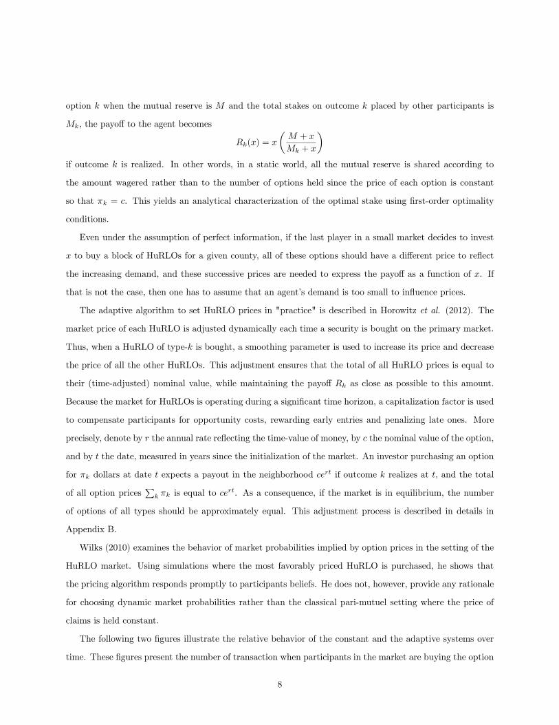
Even under the assumption of perfect information, if the last player in a small market decides to invest

to buy a block of HuRLOs for a given county, all of these options should have a different price to reflect

the increasing demand, and these successive prices are needed to express the payoff as a function of . If

that is not the case, then one has to assume that an agent’s demand is too small to influence prices.

The adaptive algorithm to set HuRLO prices in "practice" is described in Horowitz et al. (2012). The

market price of each HuRLO is adjusted dynamically each time a security is bought on the primary market.

Thus, when a HuRLO of type- is bought, a smoothing parameter is used to increase its price and decrease

the price of all the other HuRLOs. This adjustment ensures that the total of all HuRLO prices is equal to

their (time-adjusted) nominal value, while maintaining the payoff as close as possible to this amount.

Because the market for HuRLOs is operating during a significant time horizon, a capitalization factor is used

to compensate participants for opportunity costs, rewarding early entries and penalizing late ones. More

precisely, denote by the annual rate reflecting the time-value of money, by the nominal value of the option,

and by the date, measured in years since the initialization of the market. An investor purchasing an option

for dollars at date expects a payout in the neighborhood if outcome realizes at , and the total

of all option pricesP

is equal to . As a consequence, if the market is in equilibrium, the number

of options of all types should be approximately equal. This adjustment process is described in details in

Appendix B.

Wilks (2010) examines the behavior of market probabilities implied by option prices in the setting of the

HuRLO market. Using simulations where the most favorably priced HuRLO is purchased, he shows that

the pricing algorithm responds promptly to participants beliefs. He does not, however, provide any rationale

for choosing dynamic market probabilities rather than the classical pari-mutuel setting where the price of

claims is held constant.

The following two figures illustrate the relative behavior of the constant and the adaptive systems over

time. These figures present the number of transaction when participants in the market are buying the option

8

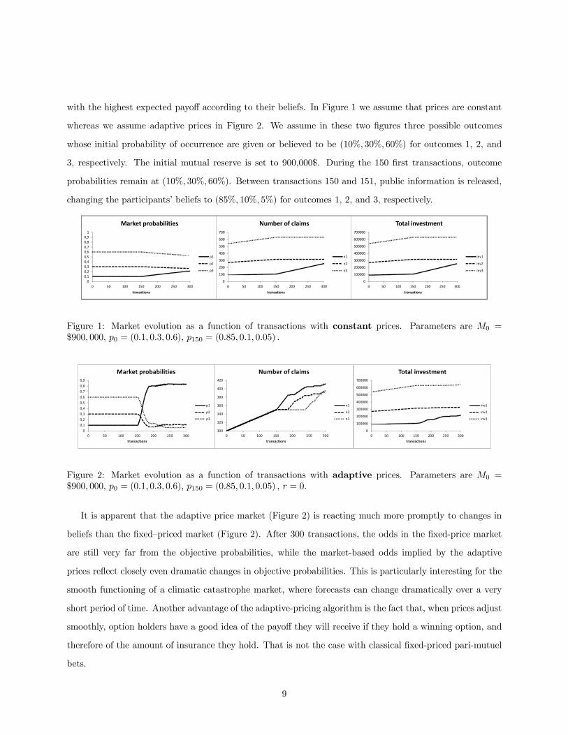
with the highest expected payoff according to their beliefs. In Figure 1 we assume that prices are constant

whereas we assume adaptive prices in Figure 2. We assume in these two figures three possible outcomes

whose initial probability of occurrence are given or believed to be (10% 30% 60%) for outcomes 1, 2, and

3, respectively. The initial mutual reserve is set to 900,000$. During the 150 first transactions, outcome

probabilities remain at (10% 30% 60%). Between transactions 150 and 151, public information is released,

changing the participants’ beliefs to (85% 10% 5%) for outcomes 1, 2, and 3, respectively.

0

0,1

0,2

0,3

0,4

0,5

0,6

0,7

0,8

0,9

1

0 50 100 150 200 250 300

transations

Market probabilities

p1

p2

p3

0

100

200

300

400

500

600

700

0 50 100 150 200 250 300

transations

Number of claims

n1

n2

n3

0

100000

200000

300000

400000

500000

600000

700000

0 50 100 150 200 250 300

transations

Total investment

inv1

inv2

inv3

Figure 1: Market evolution as a function of transactions with constant prices. Parameters are 0 =

$900 000, 0 = (01 03 06) 150 = (085 01 005)

0

0,1

0,2

0,3

0,4

0,5

0,6

0,7

0,8

0,9

0 50 100 150 200 250 300

transactions

Market probabilities

p1

p2

p3

300

320

340

360

380

400

420

0 50 100 150 200 250 300

transactions

Number of claims

n1

n2

n3

0

100000

200000

300000

400000

500000

600000

700000

0 50 100 150 200 250 300

transactions

Total investment

inv1

inv2

inv3

Figure 2: Market evolution as a function of transactions with adaptive prices. Parameters are 0 =

$900 000, 0 = (01 03 06) 150 = (085 01 005) = 0

It is apparent that the adaptive price market (Figure 2) is reacting much more promptly to changes in

beliefs than the fixed—priced market (Figure 2). After 300 transactions, the odds in the fixed-price market

are still very far from the objective probabilities, while the market-based odds implied by the adaptive

prices reflect closely even dramatic changes in objective probabilities. This is particularly interesting for the

smooth functioning of a climatic catastrophe market, where forecasts can change dramatically over a very

short period of time. Another advantage of the adaptive-pricing algorithm is the fact that, when prices adjust

smoothly, option holders have a good idea of the payoff they will receive if they hold a winning option, and

therefore of the amount of insurance they hold. That is not the case with classical fixed-priced pari-mutuel

bets.

9

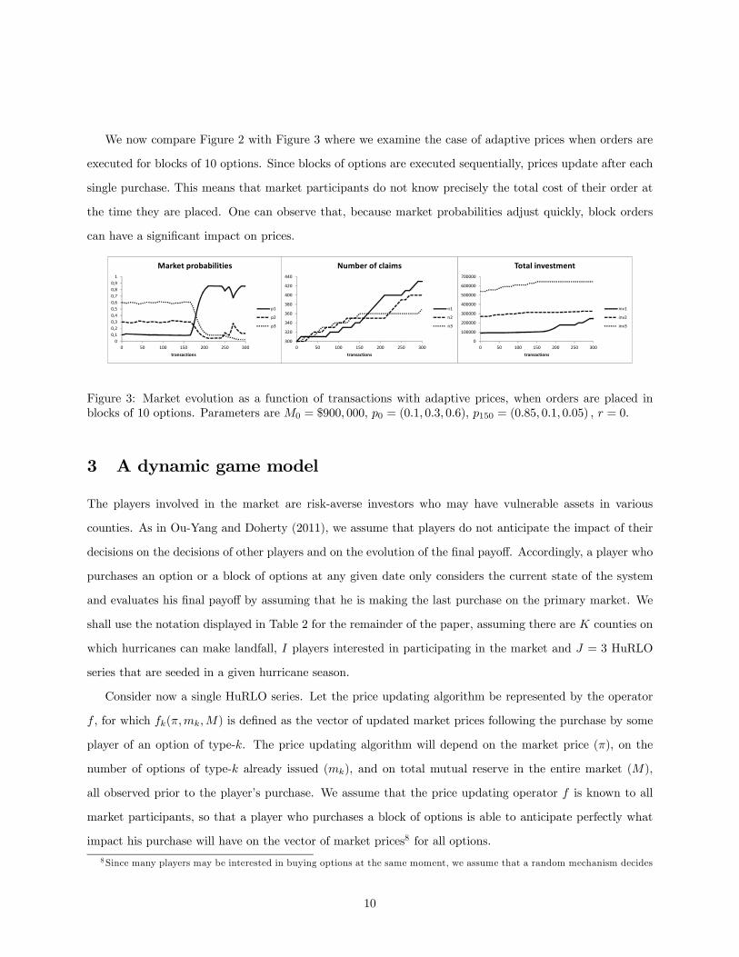
We now compare Figure 2 with Figure 3 where we examine the case of adaptive prices when orders are

executed for blocks of 10 options. Since blocks of options are executed sequentially, prices update after each

single purchase. This means that market participants do not know precisely the total cost of their order at

the time they are placed. One can observe that, because market probabilities adjust quickly, block orders

can have a significant impact on prices.

0

0,1

0,2

0,3

0,4

0,5

0,6

0,7

0,8

0,9

1

0 50 100 150 200 250 300

transactions

Market probabilities

p1

p2

p3

300

320

340

360

380

400

420

440

0 50 100 150 200 250 300

transactions

Number of claims

n1

n2

n3

0

100000

200000

300000

400000

500000

600000

700000

0 50 100 150 200 250 300

transactions

Total investment

inv1

inv2

inv3

Figure 3: Market evolution as a function of transactions with adaptive prices, when orders are placed in

blocks of 10 options. Parameters are 0 = $900 000, 0 = (01 03 06) 150 = (085 01 005) = 0

3 A dynamic game model

The players involved in the market are risk-averse investors who may have vulnerable assets in various

counties. As in Ou-Yang and Doherty (2011), we assume that players do not anticipate the impact of their

decisions on the decisions of other players and on the evolution of the final payoff. Accordingly, a player who

purchases an option or a block of options at any given date only considers the current state of the system

and evaluates his final payoff by assuming that he is making the last purchase on the primary market. We

shall use the notation displayed in Table 2 for the remainder of the paper, assuming there are counties on

which hurricanes can make landfall, players interested in participating in the market and = 3 HuRLO

series that are seeded in a given hurricane season.

Consider now a single HuRLO series. Let the price updating algorithm be represented by the operator

, for which () is defined as the vector of updated market prices following the purchase by some

player of an option of type-. The price updating algorithm will depend on the market price (), on the

number of options of type- already issued (), and on total mutual reserve in the entire market (),

all observed prior to the player’s purchase. We assume that the price updating operator is known to all

market participants, so that a player who purchases a block of options is able to anticipate perfectly what

impact his purchase will have on the vector of market prices8 for all options.

8Since many players may be interested in buying options at the same moment, we assume that a random mechanism decides

10

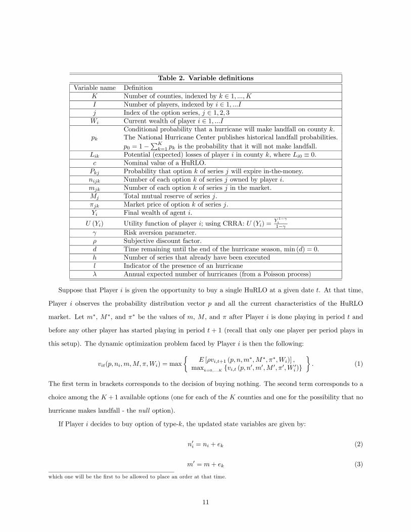
Table 2. Variable definitions

Variable name Definition

Number of counties, indexed by ∈ 1 Number of players, indexed by ∈ 1 Index of the option series, ∈ 1 2 3 Current wealth of player ∈ 1

Conditional probability that a hurricane will make landfall on county .

The National Hurricane Center publishes historical landfall probabilities.

0 = 1−P

=1 is the probability that it will not make landfall.

Potential (expected) losses of player in county , where 0 ≡ 0 Nominal value of a HuRLO.

Probability that option of series will expire in-the-money.

Number of each option of series owned by player .

Number of each option of series in the market.

Total mutual reserve of series .

Market price of option of series .

Final wealth of agent .

() Utility function of player ; using CRRA: () =1−

1− Risk aversion parameter.

Subjective discount factor.

Time remaining until the end of the hurricane season, min () = 0.

Number of series that already have been executed

Indicator of the presence of an hurricane

Annual expected number of hurricanes (from a Poisson process)

Suppose that Player is given the opportunity to buy a single HuRLO at a given date . At that time,

Player observes the probability distribution vector and all the current characteristics of the HuRLO

market. Let ∗, ∗, and ∗ be the values of , , and after Player is done playing in period and

before any other player has started playing in period + 1 (recall that only one player per period plays in

this setup). The dynamic optimization problem faced by Player is then the following:

( ) = max

½ [+1 (

∗∗ ∗)]

max=0

{ ( 00 0 0 0 )}

¾ (1)

The first term in brackets corresponds to the decision of buying nothing. The second term corresponds to a

choice among the +1 available options (one for each of the counties and one for the possibility that no

hurricane makes landfall - the null option).

If Player decides to buy option of type-, the updated state variables are given by:

0 = + (2)

0 = + (3)

which one will be the first to be allowed to place an order at that time.

11

0 = + · (4)

0 = () (5)

0 = − · (6)

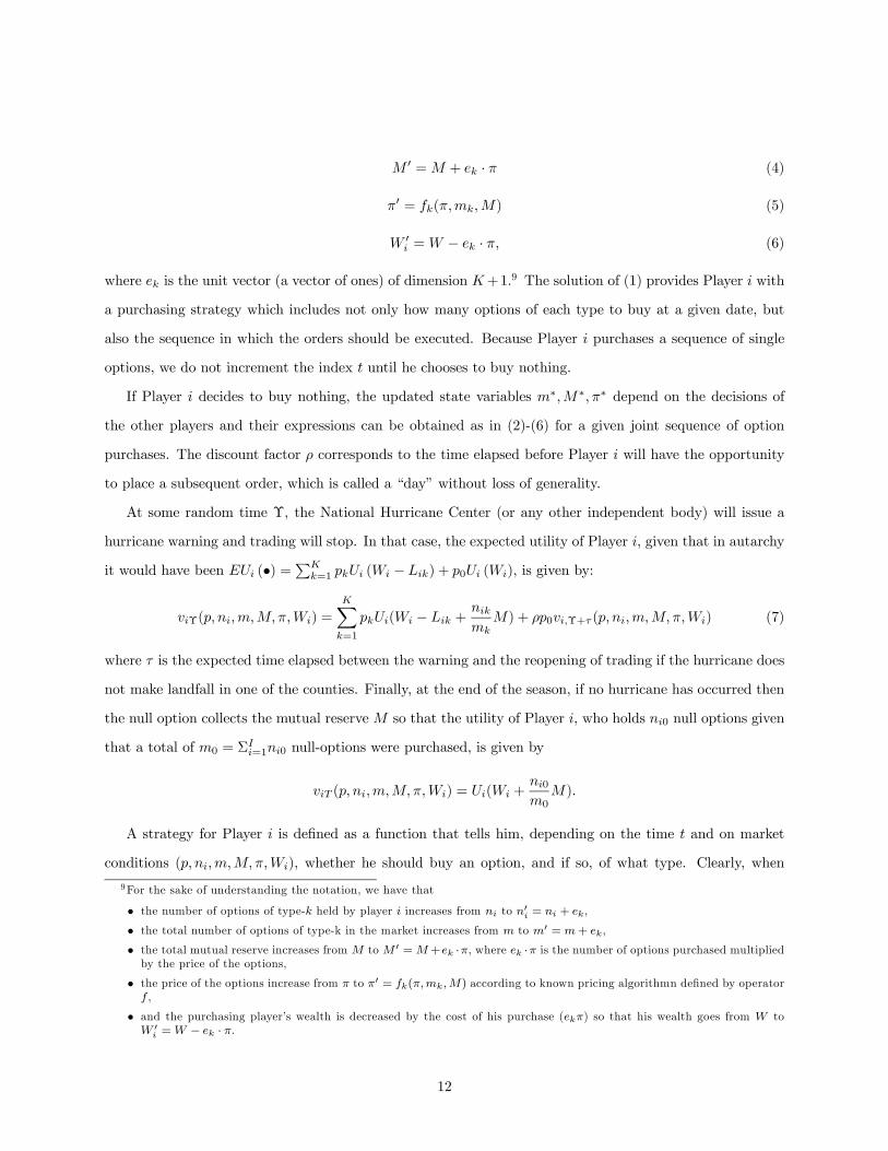
where is the unit vector (a vector of ones) of dimension +1.9 The solution of (1) provides Player with

a purchasing strategy which includes not only how many options of each type to buy at a given date, but

also the sequence in which the orders should be executed. Because Player purchases a sequence of single

options, we do not increment the index until he chooses to buy nothing.

If Player decides to buy nothing, the updated state variables ∗∗ ∗ depend on the decisions of

the other players and their expressions can be obtained as in (2)-(6) for a given joint sequence of option

purchases. The discount factor corresponds to the time elapsed before Player will have the opportunity

to place a subsequent order, which is called a “day” without loss of generality.

At some random time Υ, the National Hurricane Center (or any other independent body) will issue a

hurricane warning and trading will stop. In that case, the expected utility of Player , given that in autarchy

it would have been (•) =P

=1 ( − ) + 0 (), is given by:

Υ( ) =

X=1

( − +

) + 0Υ+ ( ) (7)

where is the expected time elapsed between the warning and the reopening of trading if the hurricane does

not make landfall in one of the counties. Finally, at the end of the season, if no hurricane has occurred then

the null option collects the mutual reserve so that the utility of Player , who holds 0 null options given

that a total of 0 = Σ=10 null-options were purchased, is given by

( ) = ( +0

0

)

A strategy for Player is defined as a function that tells him, depending on the time and on market

conditions ( ), whether he should buy an option, and if so, of what type. Clearly, when

9For the sake of understanding the notation, we have that

• the number of options of type- held by player increases from to 0 = + ,

• the total number of options of type-k in the market increases from to 0 = + ,

• the total mutual reserve increases from to 0 =+ ·, where · is the number of options purchased multipliedby the price of the options,

• the price of the options increase from to 0 = () according to known pricing algorithmn defined by operator

,

• and the purchasing player’s wealth is decreased by the cost of his purchase () so that his wealth goes from to

0 = − · .

12

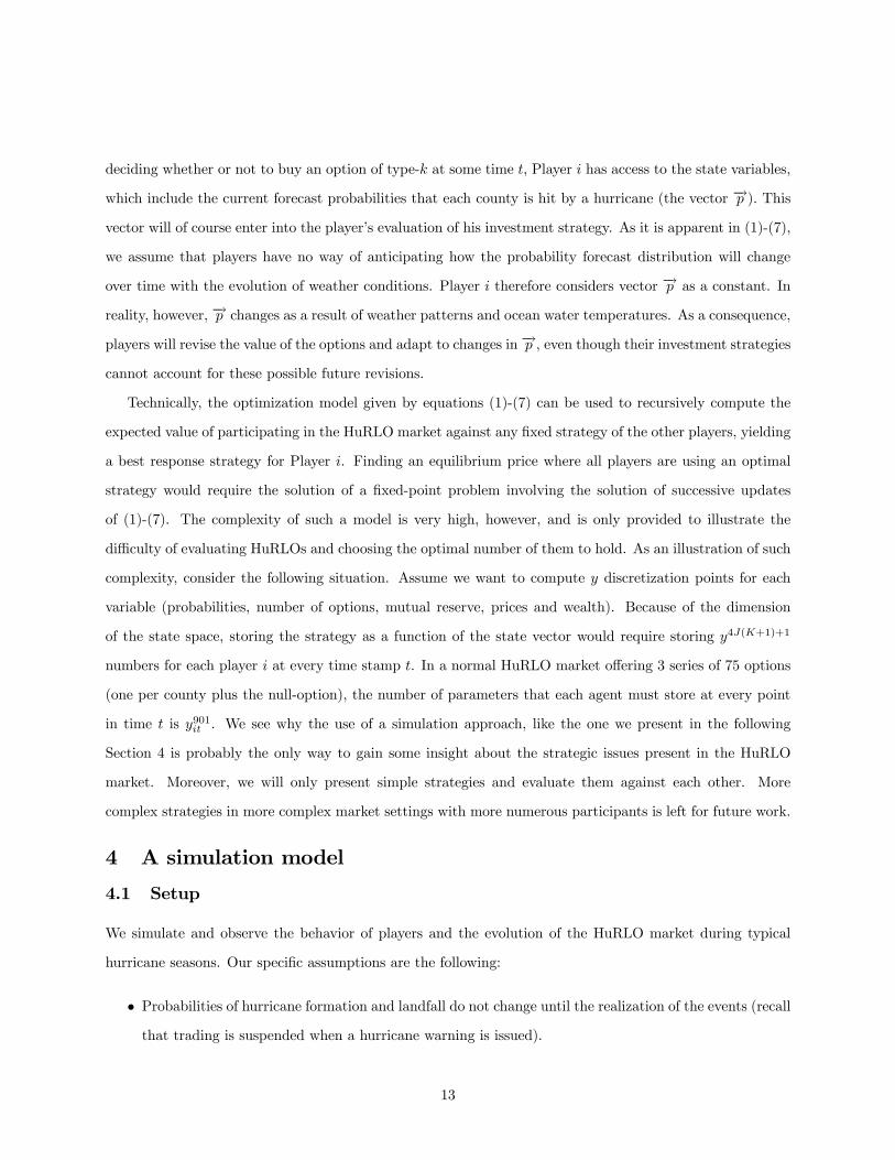
deciding whether or not to buy an option of type- at some time Player has access to the state variables,

which include the current forecast probabilities that each county is hit by a hurricane (the vector −→ ). Thisvector will of course enter into the player’s evaluation of his investment strategy. As it is apparent in (1)-(7),

we assume that players have no way of anticipating how the probability forecast distribution will change

over time with the evolution of weather conditions. Player therefore considers vector −→ as a constant. In

reality, however, −→ changes as a result of weather patterns and ocean water temperatures. As a consequence,players will revise the value of the options and adapt to changes in −→ , even though their investment strategiescannot account for these possible future revisions.

Technically, the optimization model given by equations (1)-(7) can be used to recursively compute the

expected value of participating in the HuRLO market against any fixed strategy of the other players, yielding

a best response strategy for Player . Finding an equilibrium price where all players are using an optimal

strategy would require the solution of a fixed-point problem involving the solution of successive updates

of (1)-(7). The complexity of such a model is very high, however, and is only provided to illustrate the

difficulty of evaluating HuRLOs and choosing the optimal number of them to hold. As an illustration of such

complexity, consider the following situation. Assume we want to compute discretization points for each

variable (probabilities, number of options, mutual reserve, prices and wealth). Because of the dimension

of the state space, storing the strategy as a function of the state vector would require storing 4(+1)+1

numbers for each player at every time stamp . In a normal HuRLO market offering 3 series of 75 options

(one per county plus the null-option), the number of parameters that each agent must store at every point

in time is 901 . We see why the use of a simulation approach, like the one we present in the following

Section 4 is probably the only way to gain some insight about the strategic issues present in the HuRLO

market. Moreover, we will only present simple strategies and evaluate them against each other. More

complex strategies in more complex market settings with more numerous participants is left for future work.

4 A simulation model

4.1 Setup

We simulate and observe the behavior of players and the evolution of the HuRLO market during typical

hurricane seasons. Our specific assumptions are the following:

• Probabilities of hurricane formation and landfall do not change until the realization of the events (recallthat trading is suspended when a hurricane warning is issued).

13

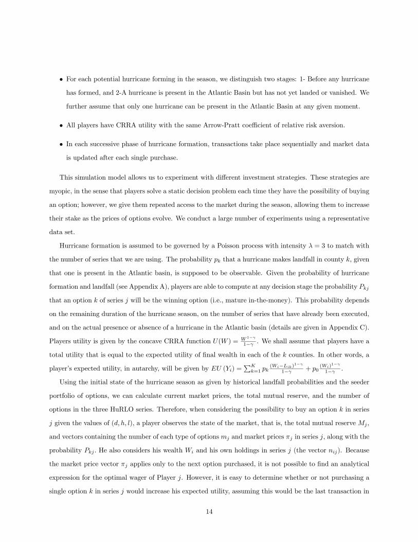
• For each potential hurricane forming in the season, we distinguish two stages: 1- Before any hurricanehas formed, and 2-A hurricane is present in the Atlantic Basin but has not yet landed or vanished. We

further assume that only one hurricane can be present in the Atlantic Basin at any given moment.

• All players have CRRA utility with the same Arrow-Pratt coefficient of relative risk aversion.

• In each successive phase of hurricane formation, transactions take place sequentially and market datais updated after each single purchase.

This simulation model allows us to experiment with different investment strategies. These strategies are

myopic, in the sense that players solve a static decision problem each time they have the possibility of buying

an option; however, we give them repeated access to the market during the season, allowing them to increase

their stake as the prices of options evolve. We conduct a large number of experiments using a representative

data set.

Hurricane formation is assumed to be governed by a Poisson process with intensity = 3 to match with

the number of series that we are using. The probability that a hurricane makes landfall in county , given

that one is present in the Atlantic basin, is supposed to be observable. Given the probability of hurricane

formation and landfall (see Appendix A), players are able to compute at any decision stage the probability

that an option of series will be the winning option (i.e., mature in-the-money). This probability depends

on the remaining duration of the hurricane season, on the number of series that have already been executed,

and on the actual presence or absence of a hurricane in the Atlantic basin (details are given in Appendix C).

Players utility is given by the concave CRRA function ( ) = 1−1− . We shall assume that players have a

total utility that is equal to the expected utility of final wealth in each of the counties. In other words, a

player’s expected utility, in autarchy, will be given by () =P

=1 (−)1−

1− + 0()

1−

1− .

Using the initial state of the hurricane season as given by historical landfall probabilities and the seeder

portfolio of options, we can calculate current market prices, the total mutual reserve, and the number of

options in the three HuRLO series. Therefore, when considering the possibility to buy an option in series

given the values of ( ), a player observes the state of the market, that is, the total mutual reserve

and vectors containing the number of each type of options and market prices in series , along with the

probability He also considers his wealth and his own holdings in series (the vector ). Because

the market price vector applies only to the next option purchased, it is not possible to find an analytical

expression for the optimal wager of Player . However, it is easy to determine whether or not purchasing a

single option in series would increase his expected utility, assuming this would be the last transaction in

14

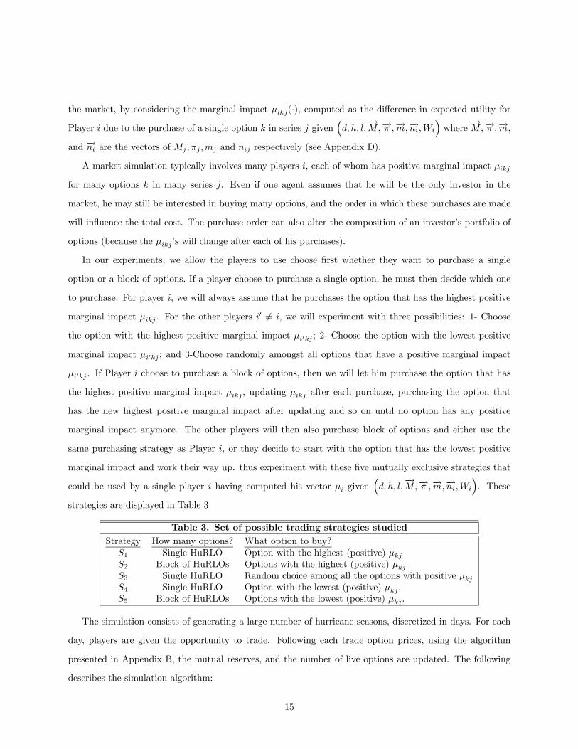
the market, by considering the marginal impact (·), computed as the difference in expected utility forPlayer due to the purchase of a single option in series given

³

−→−→ −→−→

´where

−→−→ −→

and −→ are the vectors of and respectively (see Appendix D).

A market simulation typically involves many players , each of whom has positive marginal impact

for many options in many series . Even if one agent assumes that he will be the only investor in the

market, he may still be interested in buying many options, and the order in which these purchases are made

will influence the total cost. The purchase order can also alter the composition of an investor’s portfolio of

options (because the ’s will change after each of his purchases).

In our experiments, we allow the players to use choose first whether they want to purchase a single

option or a block of options. If a player choose to purchase a single option, he must then decide which one

to purchase. For player , we will always assume that he purchases the option that has the highest positive

marginal impact . For the other players 0 6= , we will experiment with three possibilities: 1- Choose

the option with the highest positive marginal impact 0 ; 2- Choose the option with the lowest positive

marginal impact 0 ; and 3-Choose randomly amongst all options that have a positive marginal impact

0 . If Player choose to purchase a block of options, then we will let him purchase the option that has

the highest positive marginal impact , updating after each purchase, purchasing the option that

has the new highest positive marginal impact after updating and so on until no option has any positive

marginal impact anymore. The other players will then also purchase block of options and either use the

same purchasing strategy as Player , or they decide to start with the option that has the lowest positive

marginal impact and work their way up. thus experiment with these five mutually exclusive strategies that

could be used by a single player having computed his vector given³

−→−→ −→−→

´. These

strategies are displayed in Table 3

Table 3. Set of possible trading strategies studied

Strategy How many options? What option to buy?

1 Single HuRLO Option with the highest (positive) 2 Block of HuRLOs Options with the highest (positive) 3 Single HuRLO Random choice among all the options with positive 4 Single HuRLO Option with the lowest (positive)

5 Block of HuRLOs Options with the lowest (positive)

The simulation consists of generating a large number of hurricane seasons, discretized in days. For each

day, players are given the opportunity to trade. Following each trade option prices, using the algorithm

presented in Appendix B, the mutual reserves, and the number of live options are updated. The following

describes the simulation algorithm:

15

Algorithm

1. Read parameters and initialize the market using , yielding 0 and 0. Initialize the options held by

all players to 0 = 0 for = 1 and = 0 Set = 1, = 0 and = 0

2. Using the hurricane model, generate hurricane dates, durations and outcomes during the hurricane

season.

3. Compute probabilities at ( ) and select randomly an ordering O of the players.

4. For = 1

(a) Determine the purchase order for Player O() according to his strategy

(b) For each transaction by Player O(), update market variables

(c) When purchase order of Player O() is completed, set = + 1.

5. If = 0 stop. Otherwise, update and according to the hurricane scenario realization. Set =

− 1365 and go to 3.

4.2 General results from the simulations

We present the evolution of the market under various scenarios about the strategies used by the players. We

thus report representative results obtained with a model involving 4 players, 4 counties at risk for a hurricane

landfall, and 3 option series. The HuRLO market is initialized with an initial mutual reserve of $1,000,000

used to purchase an equal number of each options at prices set to what can be viewed as historical landfall

probabilities. For the sake of the simulation, these landfall probabilities are set to 1 = 02 2 = 015

3 = 025 4 = 022. The complement, which corresponds to the probability that a given hurricane does not

make landfall is given by 0 = 1 − Σ4=1 = 018, assumed constant over the hurricane year. Parameter

values are = 1000 = 0 and = 05 and a seeding fee of 3% is taken from the mutual reserve at a

settlement date. Results are based on 200 repetitions of the simulation algorithm.

We conducted five experiments using the same simulation data (200 trials) to assess whether the HuRLO-

purchasing strategies have any significant impact on the market as a whole. In experiments 1 and 2 all

players use the same strategy, while in experiments 3, 4, and 5, Player 1 is using a different strategy

than the others. Table 4 presents the set of experiments as a function of the set of possible trading situations

presented in Table 3.

16

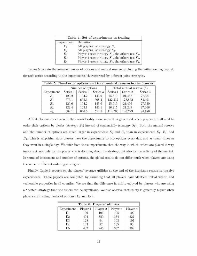
Table 4. Set of experiments in trading

Experiment Definition

1 All players use strategy 1.

2 All players use strategy 2.

3 Player 1 uses strategy 1, the others use 3.

4 Player 1 uses strategy 1, the others use 4.

5 Player 1 uses strategy 2, the others use 5.

Tables 5 contain the average number of options and mutual reserve, excluding the initial seeding capital,

for each series according to the experiments, characterized by different joint strategies.

Table 5: Number of options and total mutual reserve in the 3 series

Number of options Total mutual reserve ($)

Experiment Series 1 Series 2 Series 3 Series 1 Series 2 Series 3

1 120.2 104.2 143.9 25,810 21,467 27,381

2 676.1 655.6 508.4 122,337 128,852 84,491

3 120.6 104.2 145.6 25,919 21,456 27,630

4 122.4 103.1 143.1 26,315 21,249 27,266

5 682.1 646.6 512.5 114,766 126,723 84,786

A first obvious conclusion is that considerably more interest is generated when players are allowed to

order their options by blocks (strategy 2) instead of sequentially (strategy 1). Both the mutual reserve

and the number of options are much larger in experiments 2 and 5 than in experiments 1, 3, and

4. This is surprising since players have the opportunity to buy options every day, and as many times as

they want in a single day. We infer from these experiments that the way in which orders are placed is very

important, not only for the player who is deciding about his strategy, but also for the activity of the market.

In terms of investment and number of options, the global results do not differ much when players are using

the same or different ordering strategies.

Finally, Table 6 reports on the players’ average utilities at the end of the hurricane season in the five

experiments. These payoffs are computed by assuming that all players have identical initial wealth and

vulnerable properties in all counties. We see that the difference in utility enjoyed by players who are using

a “better” strategy than the others can be significant. We also observe that utility is generally higher when

players are trading blocks of options (2 and 5).

Table 6: Players’ utilities

Experiment Player 1 Player 2 Player 3 Player 4

E1 109 106 105 109

E2 404 359 334 327

E3 128 94 103 107

E4 143 92 105 90

E5 402 246 337 399

17

From these experiments, we can conclude that, if one decides to participate in the HuRLO market, the

timing and ordering of his option purchases is important, even when all players are myopic. Finding the best

response to fixed strategies of other players, or the equilibrium strategy in a market populated by rational

farsighted players may however be a very difficult problem, as we show in the next section.

4.3 One example

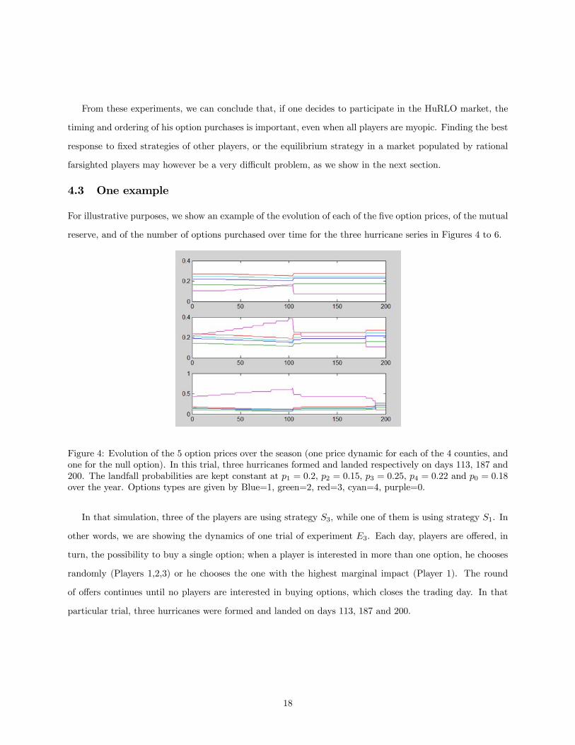
For illustrative purposes, we show an example of the evolution of each of the five option prices, of the mutual

reserve, and of the number of options purchased over time for the three hurricane series in Figures 4 to 6.

Figure 4: Evolution of the 5 option prices over the season (one price dynamic for each of the 4 counties, and

one for the null option). In this trial, three hurricanes formed and landed respectively on days 113, 187 and

200. The landfall probabilities are kept constant at 1 = 02 2 = 015 3 = 025 4 = 022 and 0 = 018

over the year. Options types are given by Blue=1, green=2, red=3, cyan=4, purple=0.

In that simulation, three of the players are using strategy 3, while one of them is using strategy 1. In

other words, we are showing the dynamics of one trial of experiment 3. Each day, players are offered, in

turn, the possibility to buy a single option; when a player is interested in more than one option, he chooses

randomly (Players 1,2,3) or he chooses the one with the highest marginal impact (Player 1). The round

of offers continues until no players are interested in buying options, which closes the trading day. In that

particular trial, three hurricanes were formed and landed on days 113, 187 and 200.

18

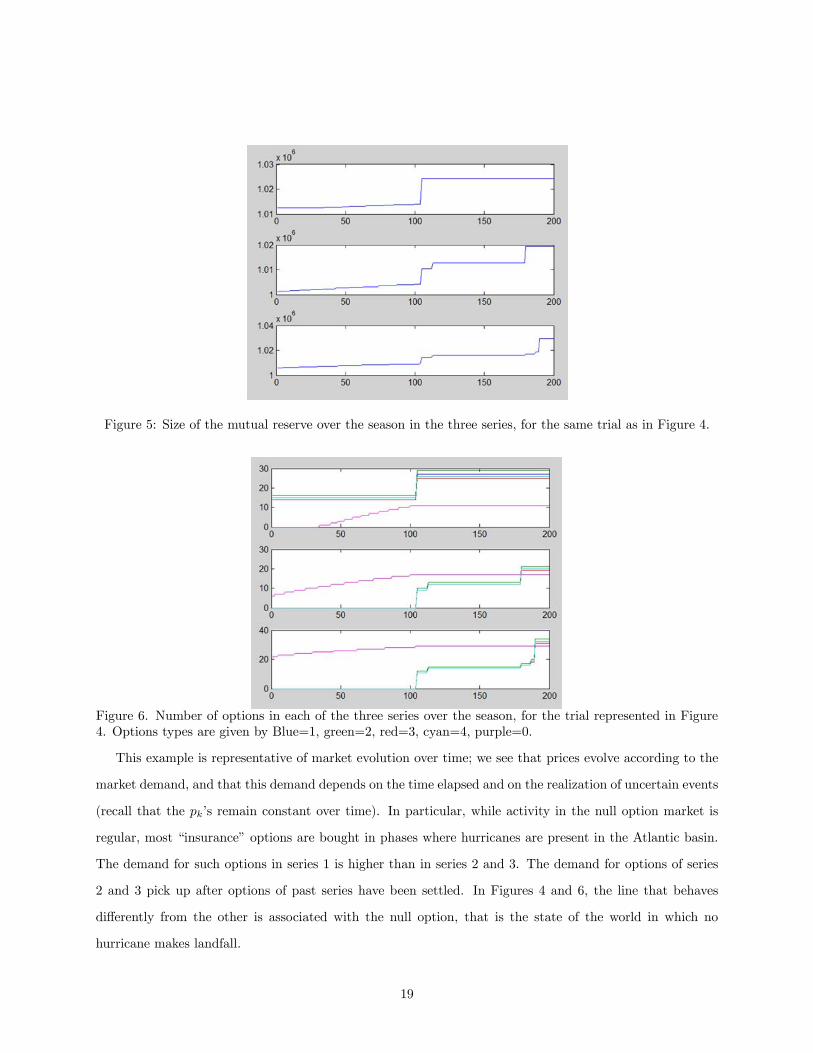
Figure 5: Size of the mutual reserve over the season in the three series, for the same trial as in Figure 4.

Figure 6. Number of options in each of the three series over the season, for the trial represented in Figure

4. Options types are given by Blue=1, green=2, red=3, cyan=4, purple=0.

This example is representative of market evolution over time; we see that prices evolve according to the

market demand, and that this demand depends on the time elapsed and on the realization of uncertain events

(recall that the ’s remain constant over time). In particular, while activity in the null option market is

regular, most “insurance” options are bought in phases where hurricanes are present in the Atlantic basin.

The demand for such options in series 1 is higher than in series 2 and 3. The demand for options of series

2 and 3 pick up after options of past series have been settled. In Figures 4 and 6, the line that behaves

differently from the other is associated with the null option, that is the state of the world in which no

hurricane makes landfall.

19

5 Conclusion

Pari-mutuel insurance have several merits with respect to insurance markets as pointed out by Ou-Yang

and Doherty (2011). In particular pari-mutuel insurance should be an interesting alternative to traditional

insurance when the latter has high transaction costs, is too expensive, and is plagued with informational

problems, or when it is simply not available. With respect to the Florida catastrophic and weather risk

market, the development of such an alternative to traditional insurance products would appear to have a

high potential. One could even imagine that the Florida market would be ready for the introduction of such

a risk management tool that is neither plagued by moral hazard nor adverse selection problems. Moreover, in

an active HuRLO market insurers would bear no counterparty or default risk, and they do not need to invest

in further loss and cost appraisals. That is why it was natural to think, in 2008 when such a market was

introduced, that HuRLOs would perform well in Florida. Unfortunately, HuRLOs are not pure pari-mutuel

insurance products since the payoff of the option does not depend directly on the amount wagered.

The aim of this paper was to investigate whether there are strategic issues when a player decides to invest

in HuRLOs. We showed that the order, sequence, and packaging of transactions have non-trivial impacts on

the price paid and on the number of options held by players. This highlights a major drawback of HuRLOs as

an insurance product, that is, HuRLOs are very difficult to evaluate and to purchase optimally. In addition,

it is important to note that speculators are really needed for the HuRLO market to work. Indeed, if the only

options bought correspond to counties where the hurricane risk is high, then there is a real possibility that

properties in these counties will be under-insured. In the limit, if there is only one county where hurricanes

can strike, then without speculators buying the null option, there is no insurance at all because what the

investors will recover will be exactly what they put in the pool.

As a last remark, we would like to point out that we did not consider the choice between buying insurance

or buying options in the sense that we assume that the only available hedge against losses are the HuRLOs.

Also, we did not examine in our simulations whether market participants would prefer to acquire other types

of securities; we assumed that investors could only buy HuRLOs, and they would do so whenever it would

increase their expected utility. The choice between traditional and pari-mutuel insurance may be simplified

somewhat if one assumes that the payoff of a winning option should be near its par value in a well-functioning

market. However, the question of how and when to buy pari-mutuel insurance remains open.

20

6 Appendices

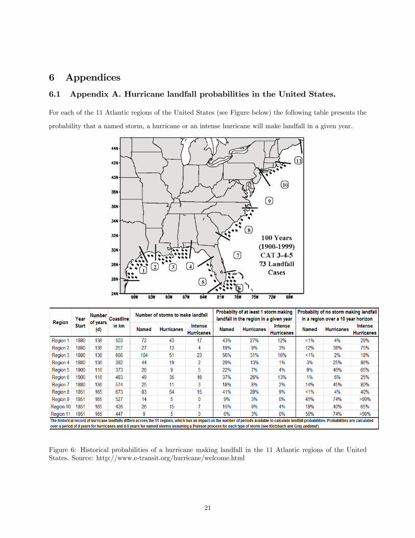
6.1 Appendix A. Hurricane landfall probabilities in the United States.

For each of the 11 Atlantic regions of the United States (see Figure below) the following table presents the

probability that a named storm, a hurricane or an intense hurricane will make landfall in a given year.

Figure 6: Historical probabilities of a hurricane making landfall in the 11 Atlantic regions of the United

States. Source: http://www.e-transit.org/hurricane/welcome.html

21

Under a Poisson distribution, the probability that at least one storm makes landfall is given by the

complement probability that no storm makes landfall: 1− (0) = 1− 1

, where is the number of named

storms or hurricanes or intense hurricane to make landfall in that particular region over a span of years

according to historical records. Historical records differ by region, which has an impact on the number of

hurricanes and named storms that have been recorded; the impact on the empirical probability of a storm

making landfall should be small, however.

22

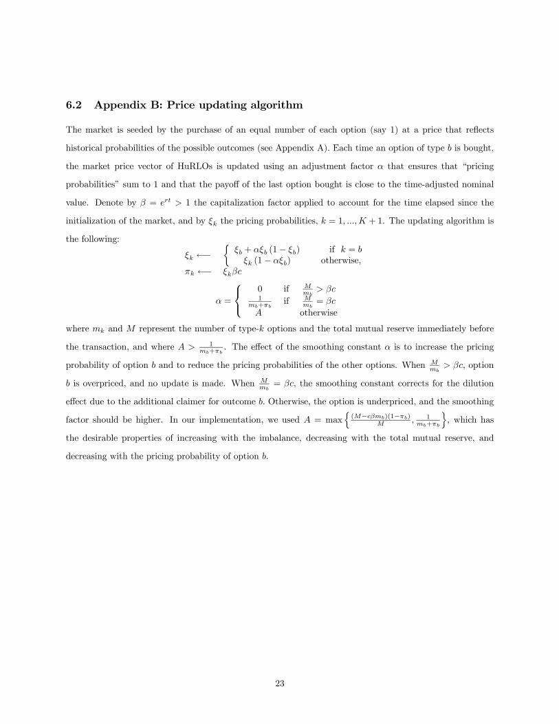
6.2 Appendix B: Price updating algorithm

The market is seeded by the purchase of an equal number of each option (say 1) at a price that reflects

historical probabilities of the possible outcomes (see Appendix A). Each time an option of type is bought,

the market price vector of HuRLOs is updated using an adjustment factor that ensures that “pricing

probabilities” sum to 1 and that the payoff of the last option bought is close to the time-adjusted nominal

value. Denote by = 1 the capitalization factor applied to account for the time elapsed since the

initialization of the market, and by the pricing probabilities, = 1 + 1. The updating algorithm is

the following:

←−½

+ (1− )

(1− )

if =

otherwise,

←−

=

⎧⎨⎩0 if

1+

if =

otherwise

where and represent the number of type- options and the total mutual reserve immediately before

the transaction, and where 1+

. The effect of the smoothing constant is to increase the pricing

probability of option and to reduce the pricing probabilities of the other options. When

, option

is overpriced, and no update is made. When

= , the smoothing constant corrects for the dilution

effect due to the additional claimer for outcome Otherwise, the option is underpriced, and the smoothing

factor should be higher. In our implementation, we used = maxn(−)(1−)

1+

o, which has

the desirable properties of increasing with the imbalance, decreasing with the total mutual reserve, and

decreasing with the pricing probability of option .

23

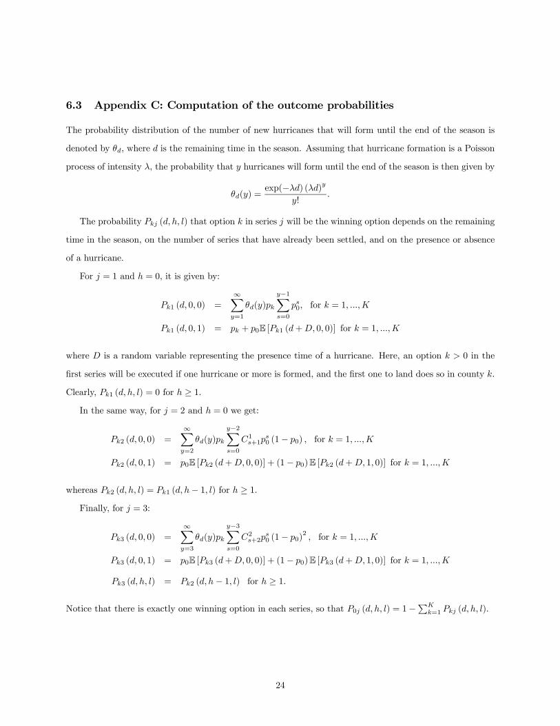
6.3 Appendix C: Computation of the outcome probabilities

The probability distribution of the number of new hurricanes that will form until the end of the season is

denoted by where is the remaining time in the season. Assuming that hurricane formation is a Poisson

process of intensity , the probability that hurricanes will form until the end of the season is then given by

() =exp(−) ()

!

The probability ( ) that option in series will be the winning option depends on the remaining

time in the season, on the number of series that have already been settled, and on the presence or absence

of a hurricane.

For = 1 and = 0, it is given by:

1 ( 0 0) =

∞X=1

()

−1X=0

0 for = 1

1 ( 0 1) = + 0E [1 (+ 0 0)] for = 1

where is a random variable representing the presence time of a hurricane. Here, an option 0 in the

first series will be executed if one hurricane or more is formed, and the first one to land does so in county .

Clearly, 1 ( ) = 0 for ≥ 1In the same way, for = 2 and = 0 we get:

2 ( 0 0) =

∞X=2

()

−2X=0

1+10 (1− 0) for = 1

2 ( 0 1) = 0E [2 (+ 0 0)] + (1− 0)E [2 (+ 1 0)] for = 1

whereas 2 ( ) = 1 ( − 1 ) for ≥ 1Finally, for = 3:

3 ( 0 0) =

∞X=3

()

−3X=0

2+20 (1− 0)

2 for = 1

3 ( 0 1) = 0E [3 (+ 0 0)] + (1− 0)E [3 (+ 1 0)] for = 1

3 ( ) = 2 ( − 1 ) for ≥ 1

Notice that there is exactly one winning option in each series, so that 0 ( ) = 1−P

=1 ( ).

24

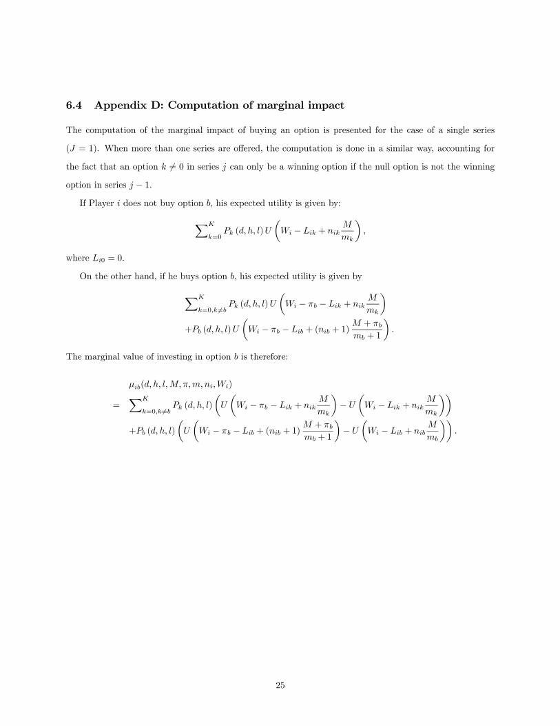
6.4 Appendix D: Computation of marginal impact

The computation of the marginal impact of buying an option is presented for the case of a single series

( = 1). When more than one series are offered, the computation is done in a similar way, accounting for

the fact that an option 6= 0 in series can only be a winning option if the null option is not the winningoption in series − 1If Player does not buy option , his expected utility is given by:

X

=0 ( )

µ − +

¶

where 0 = 0.

On the other hand, if he buys option his expected utility is given by

X

=0 6= ( )

µ − − +

¶+ ( )

µ − − + ( + 1)

+

+ 1

¶

The marginal value of investing in option is therefore:

( )

=X

=0 6= ( )

µ

µ − − +

¶−

µ − +

¶¶+ ( )

µ

µ − − + ( + 1)

+

+ 1

¶−

µ − +

¶¶

25

7 References

1. Baron, K. and J. Lange (2007). Parimutuel applications in finance: new markets for new risks, Palgrave

Macmillan.

2. Bonazzi, A., A.L. Dobbin, J.K. Turner, P.S. Wilson, C. Mitas, and E. Bellone (2014). A Simulation

Approach for Estimating Hurricane Risk over a 5-yr Horizon. Weather, Climate and Society, 6: 77-90.

3. Bove, M.C., J.B. Elsner, C.W. Landsea, X. Niu, and J.J. O’Brien (1998). Effect of El Nino of U.S.

Landfalling Hurricanes, Revisited. Bulletin of American Meteorological Society 79 : 2477-2482.

4. Cummins, J. D. (2008). CAT Bonds and Other Risk-Linked Securities: State of the Market and Recent

Developments. Risk Management and Insurance Review 11(1) : 23-47.

5. Cummins, J. D. (2012). CAT bonds and other risk-linked securities: Product design and evolution of

the market. The Geneva Reports 39.

6. Cummis, J.D. and P. Barrieu (2013). , In G. Dionne (Ed.) The Handbook of Insurance.

7. Epstein, E. S. (1985). Statistical Inference and Prediction in Climatology : A Bayesian Approach.

Meteorological Monographs 42 : 199.

8. Doherty, N. A. (1997). Financial innovation in the management of catastrophe risk. Journal of Applied

Corporate Finance 10(3) : 84-95.

9. Froot, K. A. (2001). The market for catastrophe risk: a clinical examination. Journal of Financial

Economics 60(2) : 529-571.

10. Gray, W. M., C.W. Landsea, P.W. Mielke, and K.J. Berry (1992). Prediction Atlantic Seasonal

Hurricane Activity 6-11 Months in Advance. Weather and Forecasting 7 : 440-455.

11. Gürkynak, R. and J. Wolfers (2006). Macroeconomic Derivatives : An Initial Analysis of Market-Based

Macro Forecasts, Uncertainty, and Risk. Working Paper 11929,National Bureau of Economic Research.

12. Hall, T.M. and K. Hereid (2015). The frequency and duration of U.S. hurricane droughts. Geophysical

Research Letters, 42: 3482-3485.

13. Hall, T.M. and S. Jewson (2007). Statistical modelling of North Atlantic tropical cyclone tracks. Tellus

59A(4): 486—498

26

14. Horowitz, K.A., A.L. Bequillard, A.P. Nyren, P.E. Protter, and D.S. Wilks (2012). U.S. Patent No.

8,266,042. Washington, DC: U.S. Patent and Trademark Office.

15. Jewson, S. and T.M. Hall (2007). Comparison of Local and Basin-Wide Methods for Risk Assessment

of Tropical Cyclone Landfall. Journal of Applied Meteorology and Climatology 47(2) : 361-367.

16. Kelly, D. L., D. Letson, F. Nelson, D.S. Nolan & D. Solís (2012). Evolution of subjective hurricane risk

perceptions: A Bayesian approach. Journal of Economic Behavior & Organization 81(2) : 644-663.

17. Klotzbach, P. andW. Gray (undated). United States Landfall Probability. http://www.e-transit.org/hurricane/welcome

last acccessed 28 january 2016.

18. Kriesche, B., H. Weindl, A. Smolka & V. Schmidt (2014). Stochastic simulation model for tropical

cyclone tracks with special emphasis on landfall behavior. Natural Hazards 73: 335—353

19. Kunreuther, H. and E. Michel-Kerjan (2009).

20. Lange, J. and N. Economides (2005). A Parimutuel Market Microstructure for Contingent Claims.

Journal of European Financial Management 11(1) : 25-49.

21. Meyer, R. J., M. Horowitz, D. S. Wilks, and K. A. Horowitz (2008). A Mutualized Risk Market with

Endogenous Prices, with Application to U.S. Landfalling Hurricanes. Working Paper 2008-12-08, Risk

Management and Decision Processes Center, The Wharton School of the University of Pennsylvania.

22. Meyer, R. J., M. Horowitz, D. S. Wilks, and K.A. Horowitz (2014). A Novel Financial Market For

Mitigating Hurricane Risk. II. Empirical Validation. Weather, Climate, and Society 6: 318—330.

23. Nakamura, J., U. Lall, Y. Kushnir, and B. Rajagopalan (2015): HITS: Hurricane Intensity and Track

Simulator with North Atlantic Ocean Applications for Risk Assessment. Journal of Applied Meteorol-

ogy and Climatology 54: 1620—1636.

24. Ou Yang, C. (2010). Managing Catastrophic Risk by Alternative Risk Transfer Instruments. University

of Pennsylvania Publicly accessible Dissertations 220, http://repository.upenn.edu/edissertations/220

25. Ou-Yang, C. and N. Doherty (2011). Parimutuel Insurance for Hedging against Catastrophic Risk,

Wharton School Working Paper # 2011-08.

26. Pielke Jr, R.A., J. Gratz, C.W. Landsea, D. Collins, M.A. Saunders, and R. Musulin (2008). Normalized

hurricane damage in the United States: 1900—2005. Natural Hazards Review 9(1) : 29-42.

27

27. Ramella and Madeiros (2007)

28. Rumpf J, H. Weindl, P. Höppe, E. Rauch, and V. Schmidt (2007). Stochastic modelling of tropical

cyclone tracks. Mathematical Methods of Operations Research 66(3): 475—490.

29. Rumpf J, H. Weindl, P. Höppe, E. Rauch, and V. Schmidt (2009). Tropical cyclone hazard assessment

using modelbased track simulation. Natural Hazards 48(3): 383—398.

30. SwissRe (2015). Natural catastrophes and man-made disasters in 2014: convective and winter storms

generate most losses. Sigma 2/2015, 47 pages.

31. Vickery, P. J., P. Skerlj, and L. Twisdale (2000). Simulation of Hurricane Risk in the US Using an

Empirical Track Model. Journal of Structuring Engineering 126(10) : 1222-1237.

32. Weather Risk Solutions (2013)http://www.weatherrisksolutions.com/about_us.php (January 2016).

33. Wilks, D.S. (2010). A novel financial market structure for mitigating hurricane risk. Proceedings of the

20th Conference on Probability and Statistics in the Atmospheric Sciences.

34. Yonekura E, and T.M. Hall (2011). A statistical model of tropical cyclone tracks in the western North

Pacific with ENSO-dependent cyclogenesis. Journal of Applied Meteorology and Climatology 50(8):

1725—1739

28