Embed Size (px)
Citation preview
Economics Discussion Paper Series EDP-1321
An Investigation of Oil Curse in OECD and Non-OECD Oil Exporting Economies Using
Green Measures of Income
Natina Yaduma Mika Kortelainen
Ada Wossink
October 2013
Economics School of Social Sciences
The University of Manchester Manchester M13 9PL
An Investigation of Oil Curse in OECD and Non-OECD Oil Exporting
Economies Using Green Measures of Income
Natina Yaduma1, Mika Kortelainen2 and Ada Wossink3
2013
Abstract
Empirical studies investigating the natural resource curse theory mostly employ cross-country and
panel regression techniques subject to endogeneity bias. Also, most of these studies employ GDP in
its aggregate or per-capita terms as the outcome variable in their analyses. However, the use of GDP
measures of income for resource curse investigations does not portray the true incomes of resource
intensive economies. Standard national accounts treat natural resource rents as a positive
contribution to income without making a corresponding adjustment for the value of depleted
natural resource stock. This treatment, inconsistent with green national accounting, leads to a
positive bias in the national income computations of resource rich economies. This paper deviates
from most empirical studies in the literature by using the Arellano-Bond difference GMM method in
investigating the oil curse in OECD and Non-OECD oil exporting economies. We test the robustness
of the curse in the predominantly used measures of national income, GDP, by investigating the
theme in genuine income measures of economic output as well. We employ two alternative
measures of resource intensity in our explorations: the share of oil rents in GDP and per-capita oil
reserves. Our results provide evidence of the curse in Non-OECD countries employing aggregate and
per-capita measures of genuine income. On the other hand, we find oil abundance to be a blessing
rather than a curse to the OECD countries in our sample.
JEL Classification: Q32, Q56.
Keywords: natural resource curse, GDP, genuine income, difference GMM, Hartwick rule.
1 Economics Discipline Area, School of Social Sciences, The University of Manchester, M13 9PL,
Manchester, UK. Email: [email protected] 2 Government Institute for Economic Research (VATT), P.O.Box 1279, 00101 Helsinki, Finland. Email:
[email protected] 3 Economics Discipline Area, School of Social Sciences, The University of Manchester, M13 9PL,
Manchester, UK. Email: [email protected]
1
1. Introduction
Classical economic reasoning considers vast natural resource endowments as a driver for
economic development. Sustainably managed natural resource rents could provide the finance
needed for the development of various productive assets. However, a relatively new literature
pioneered by Sachs and Warner (1995) assigns a somewhat paradoxical role to natural resource
abundance, especially for economies richly endowed with exhaustible natural resources. This
literature informs that resource scarce economies often outperform their resource rich counterparts
with higher growth rates, thus, natural resource abundance inhibits growth. The paradoxical idea
suggesting a shift from the classical conception of the growth enhancing effect of rich natural
resource endowments is termed the ‘Resource Curse’ theory. The literature ascribes the Dutch
disease, terms of trade effect, poor quality of institutions, civil conflict, rent seeking and corruption
as likely mediums through which resource abundance hinders growth (see for instance Boos and
Holm-Muller, 2012; Brunnschweiler and Bulte, 2008; Alexeev and Conrad, 2009).
As with most theoretical postulations, the resource curse theory spurred a considerable
volume of empirical studies with the objective of validating the propositions raised by its authors. A
great deal of studies exploring the subject employs the growth rate of real GDP in its aggregate or
per-capita terms as the indicator of economic progress. The choice of these income indicators
ensues from the format in which traditional national accounts presents information on aggregate
economic activity. However, the use of GDP measures in resource curse investigations is
questionable for two main reasons. First, it treats the depreciation of physical capital during the
accounting year as a positive contribution to national income.4 Thus, net domestic or net national
product is a better measure of income as it correctly adjusts for physical capital depreciation. Second
and more importantly, GDP measures of output do not portray the ‘true incomes’ of resource
intensive economies as standard national income accounting procedures are inconsistent with green
4 The popularity of GDP measurements without correcting for this depreciation might be attributed to
the following: first, there is no straightforward and objective accounting method of computing physical capital
depreciation; secondly, the incorporation of this depreciation estimate into national income accounting does
not considerably alter the GDP estimates for most countries thereby leading to very little and quite often
negligible bias in GDP accounting (see for instance, Neumayer, 2004).
We distinguish between four types of capital: (a) Natural Capital – ecosystem, mineral, oil and gas
resources and scenic views amongst others. (b) Human Capital – learned skills, health, and education amongst
others. (c) Physical Capital – plant and machinery, buildings, roads and other productive infrastructure. (d)
Intellectual Capital – a society’s culture and institutions not necessarily embodied in people and
infrastructures, for instance, legal structures that pave way for an efficient utilisation of the other forms of
capital. These can further be categorised into two major groups; natural and man-made capital, the latter
consisting of human, physical and intellectual capital.
2
accounting procedures.5 The former system of national accounts treats natural resource rents as a
positive contribution to GDP without making a corresponding adjustment to the depleted natural
capital stock. This accounting method fails to consider that the depletion of a natural resource stock
is essentially the liquidation of an asset, thus, natural resource extraction should not be treated as a
positive contribution to GDP (Hamilton and Clemens, 1999). Therefore, an accounting procedure
consistent with sustainability requires a prudential treatment of natural capital depletion in national
income accounts; this should net the sum of the value of natural resources extracted (and any
external costs associated with extraction) from the rents. Such an adjustment could considerably
reduce GDP estimates especially for resource intensive economies (Neumayer, 2004).
The adjustment of traditional national income measures to green income measures is
inextricably linked to sustainability considerations. Conceptualising sustainability as non-declining
capital stock, production possibilities, welfare or consumption overtime, Hartwick (1977) prescribed
that natural resource rents must be profitably invested in other forms of capital for development to
be sustainable. This prescription, generally referred to as the ‘Hartwick Rule’, is considered the rule
of thumb for sustainable development especially for economies with an intensive extraction of
exhaustible natural resources (Solow, 1986). Conceptually, the Hartwick rule may be more applicable
to the non-declining capital stock notion of sustainability but the prescription is not far-fetched from
the other notions as well. A non-declining capital base serves as the bedrock for non-declining
production opportunities, welfare and consumption. Thus, sustainability entails a judicious
management of an economy’s capital stock ensuring that this remains at least constant overtime.
Strict adherence to the Hartwick rule is paramount to achieving sustainable development. It is
pertinent to note that our discussion of sustainability in this paper connotes the weak but not the
strong form of sustainable development, where natural capital is almost perfectly substitutable with
man-made capital. Strong sustainability assumes only limited substitution possibilities between the
two forms of capital. We concentrate on the former in presenting a simple analysis of the
relationship between the resource curse and sustainable development using green measures of
income.
Given this background, our paper contributes to the existing empirical literature on the
resource curse in three ways. First, we investigate the curse for the most important energy resource;
crude oil. Aside the prominent role played by crude oil as an important source of energy in a great
deal of economic activities, our emphasis on this resource is not far-fetched given that it is the most
articulated to be associated with the curse (see for instance, Bjorvatn et al., 2012; Neumayer, 2004;
5 It is worth noting that our mention of the term “resource intensity” implies countries with a relatively
high share of natural resource rents in GDP.
3
Frankel, 2010). We investigate the oil curse for major OECD and Non-OECD oil producing countries.
Second, diverging from a vast majority of the empirical literature, we complement our analysis of
the curse by investigating a two-fold relationship; we investigate the (traditional) relationship
between standard measures of economic output and oil intensity on one hand, and, the relationship
between measures of sustainable development and oil intensity on the other hand. We employ the
World Bank’s green measure of income – the genuine income – as our indicator of sustainable
development. Genuine income is computationally defined as GNI less physical and natural capital
depreciation.6 It is worth noting that our paper is not the first to use this green measure of income
for investigating the curse. To our knowledge, Neumayer (2004) is probably the first and only paper
to directly employ genuine income in investigating the curse. While our paper follows Neumayer
(2004) in investigating whether or not the curse holds for genuine income measures, we employ two
competing measures of resource intensity to test the robustness of our findings. Thus, we explore
the curse using both the share of oil rents in GDP and per-capita oil reserves as the measures of
resource intensity in our explorations. The two measures effectively translate to measures of oil
dependence and abundance, respectively. The former is analogous to Neumayer (2004) and a wide
range of other studies in the resource curse literature, for instance, Bjorvatn et al. 2012; Dietz and
Neumayer 2012; Sala-i-Martin and Subramanian, 2003. The latter is in line with Brunnschweiler and
Bulte (2008) who argue for the use of stock-based measures in resource curse investigations.
Third, our paper contributes to the existing empirical literature by applying the Arellano-
Bond generalised method of moments (GMM) technique. Earlier resource curse studies often relied
on cross-country regressions and panel econometric methods (especially fixed and random effects
methods) for their investigations (see for instance Papyrakis and Gerlagh, 2004; and Neumayer,
2004). These estimation techniques are prone to endogeneity problems thereby generating
considerable scepticism on the findings arising from the use of the methods. A primary source of
endogeneity from these estimation techniques is automatically generated from the traditional
dependent variable used for the investigations, GDP. Income follows a dynamic process where its
contemporaneous observations are partly determined by their past realisations. Again, the
autoregressive term (usually defined as lagged income in growth regressions) is systematically
correlated with the errors thereby violating the OLS Gauss-Markov assumption of zero conditional
mean.7 Hence, this leads to endogeneity in resource curse models. The same problem ensues in the
presence of simultaneity, a situation where there is bi-directional causality between one or more
6 Genuine income is termed adjusted net national income in the World Bank’s books (see the World
Bank, 2011, 2012). 7 This assumption posits that the errors have an expected value of zero conditional on the regressors
(see for instance Wooldridge, 2008).
4
regressors and the dependent variable in a model. This is particularly the case where the most
commonly used measure of resource intensity, share of natural resource rents in GDP, is already
scaled by an income metric thereby automatically generating simultaneity with the income based
dependent variable. We follow Dietz et al. (2007) and Bjorvatn et al. (2012) in addressing this
problem by employing the Arellano and Bond (1991) difference GMM approach for our estimations.
The method generates a set of (weakly) exogenous regressors by instrumenting endogenous
variables with their lags (see Roodman, 2009; Arellano and Bond, 1991).
The rest of the paper is organised as follows. Section two reviews literature on the use of a
savings parallel of genuine income, the genuine savings measure, in assessing sustainability. Section
three presents the method and data for our estimations. The fourth section discusses the results,
and, the final section is dedicated to concluding remarks.
2. A Literature Survey of the Links between Genuine Savings,
Genuine Income and the Resource Curse in Assessments of
Sustainable Development
The objective of attaining non-declining wealth overtime essentially makes sustainability a
choice between present consumption and building a healthy capital base for the future generation
through strategic investments. Strict adherence to the Hartwick rule prescribing the investment of
natural resource rents in man-made capital is conceived a substantial step towards sustainability of
resource intensive economies (see for instance Solow, 1992; Hartwick, 2009). Satisfying this rule
therefore revolves around savings and investment decisions undertaken by resource rich economies.
As in GDP accounting, empirical resource curse assessments of the links between savings and
sustainable development are also not free from a major computational criticism. Traditional national
income accounts measures do not include natural capital depreciation in computations of economic
savings. For instance, an economy’s net savings is conventionally estimated by deducting only the
depreciation of physical capital from gross savings estimates. As savings is an economy’s source of
investment, and investment in turn determines the future productive base, a more accurate
estimate of savings that takes into consideration the depletion of natural resources is required for
better accounting and planning purposes. Thus, an assessment of a country’s performance towards
achieving sustainable development requires the use of green savings measures; a measure
incorporating natural capital depreciation and external costs of economic activity into savings
5
estimates of national income accounts. Amongst other reasons, this led the World Bank (1997) to
introduce the Genuine Savings measure.8 Analytically, consistently positive genuine savings
estimates indicate development may be sustainable.9 Conversely, consistently negative genuine
savings rates imply an unsustainable development path resulting in a decline in society’s wealth
overtime. This indicator is more widely employed than genuine income in assessing countries’
sustainable states. Thus, the ensuing discussion reviews a collection of studies largely employing
genuine savings indicator for sustainability assessments of oil rich countries in particular.
Kellenberg (1996) applied the genuine savings measure in investigating Ecuador’s
sustainability from 1970 to 2004. Using standard savings computations for the investigated period,
Ecuador’s savings rate was consistently more than 20 percent, with a peak of slightly greater than 30
percent in the early 1990s. However, an inclusion of Ecuador’s oil extraction and environmental
damages for estimating its genuine savings moves the true savings rate very close to zero or even
negative in some years. This implies that a shift from conventional savings calculation to genuine
savings may lead to a considerable decline in the true savings rate of resource rich countries, as in
the case of Ecuador. Ecuador had negative genuine savings rates from 1974-1990. Further, the study
found that a good proportion of the rents garnered from the exploitation of Ecuador’s oil resources
(especially in the 1970s and 1980s) has not been profitably invested in man-made capital but used to
increase consumption through various subsidy and tax-reduction policies. This finding essentially
translates to the resource curse, thus, implying an unsustainable management of Ecuador’s oil rents
when true measures of savings, and probably income, are incorporated in analysing its management
of oil rents.
Similarly, Hamilton et al. (2006) developed a Hartwick rule counterfactual framework to
investigate the amount of physical capital resource rich countries would have accumulated by 2000
if these countries had followed the Hartwick prescription since 1970. The study employed data on
investments, income and resources rents from the World Bank for its computations and analyses.
Concentrating on the results for two countries principally cited as suffering from the oil curse,
Nigeria and Venezuela, the study finds that the countries could have accumulated five and four
8 Again, it is worth noting that genuine savings is presented as adjusted net savings in the World Bank’s
publications and dataset. This measure is scaled by GDP thereby giving a ratio. The ratio is further transformed
into a percentage called genuine savings rate. Hence, the mention of genuine savings in this article translates
to genuine savings rate and vice-versa. 9 Caution must be applied in making sustainability inferences arising from positive genuine savings
rates. Positive genuine savings may not always imply a sustainable development outcome as there are certain
methodological shortcomings in genuine savings computations. Also, there are likely complications arising
from the uncertain effects of population growth and technical changes on genuine savings (see Arrow et al.,
2004, for more details).
6
times as much produced capital respectively if they had satisfied the Hartwick rule. By implication,
these countries have spent a significant amount of their oil rents on other avenues, especially
boosting current consumption, other than accumulating physical or human capital.10
Further, the
paper suggests that if Nigeria had adhered to the Hartwick rule since 1970, oil exports would not
have been as relevant as it is in the Nigerian economy today, with likely beneficial impacts on
policies diversifying the economy to other sectors.
Additionally, Hamilton and Clemens (1999) computed empirical estimates of genuine savings
rates for a wide range of countries from 1970 to 1993. The authors conceived genuine savings as net
savings plus investments in human capital less the value of natural capital depreciation and
environmental depletion. Largely employing data from the World Bank, the study finds persistently
negative genuine savings rates for a good proportion of developing countries. Not surprisingly, the
study finds negative genuine savings rate for the major oil producing developing countries in the
sample; for example, Bolivia, Ecuador, Trinidad and Tobago, Venezuela, Algeria, Bahrain, Iran
(Islamic Rep. of), Saudi Arabia, Syrian Arab Republic, and Nigeria amongst others. The authors
indicate that persistently negative genuine savings rates must eventually lead to declining wellbeing
overtime. Thus, they suggest that the link between genuine savings rates and sustainability implies
there is a wide range of policy interventions needed to attain a sustainable allocation of resource
rents, from the macroeconomic to the purely environmental.
An enquiry into probable policy measures that could be used for a sustainable management
of natural resource rents led Atkinson and Hamilton (2003) to investigate the links between resource
curse, economic growth, genuine savings and governance in a sample of 91 countries (from different
regions of the world). Applying cross-country regressions to a dataset spanning from 1980-1995
largely obtained from the World Bank, the paper regressed growth rate of GDP per-capita on initial
income (measured as 1980 GDP per-capita) to capture conditional convergence,11
resource
abundance (conceived as the share of mineral, energy and forest resources rents in GDP), a measure
of human capital (captured by average years of educational attainment of people over 25 years) and
binary variables to control for regional factors amongst other explanatory variables. The paper finds
evidence of the curse; a ten percent increase in resource abundance reduces the growth rate of GDP
by about 0.5 percent ceteris paribus. To provide an understanding of the probable underlying factors
explaining the curse, the authors interact the resource variable with three policy variables; share of
10
Closely tied to this consumption pattern is an example cited by Carbonnier and Wagner (2011)
suggesting that the construction of lavish presidential palaces and government houses often characteristic of
resource rich countries may have contributed to GDP but not to sustainable development. 11
Conditional convergence is a general idea in growth regressions that a country will enjoy faster
growth rates the further it is from its steady-state output (Barro and Sala-i-Martin, 1995).
7
government investment in GDP, share of government consumption in GDP, and share of public
sector wages and salaries in government expenditure. Most importantly, this investigation found
that resource abundant countries with a high share of government consumption in GDP on average
have lower growth rates. A further analysis found that resource rich countries that have suffered
from the curse are primarily those with low or negative genuine savings rates. Thus, the paper
recommends a shift from the dissipation of resource rents from financing current consumption to
prudent investments in man-made capital as a key policy action towards avoiding the curse. This
should gear resource intensive economies towards sustainable development.
Moreover, Dietz et al. (2007) investigated whether improving the quality of political and
bureaucratic institutions mitigates the growth impairing effect of resource dependence. The paper
employed the commonly used fixed effects estimation method complemented by the Arellano-Bond
difference GMM technique to capture the dynamic process of the outcome variable – genuine
savings – and correct for probable endogeneity. However, the endogeneity concerns embedded in
the former method led the study to draw its major findings and conclusions from the results
produced by the latter. To investigate the role of improved institutions in mitigating the curse, the
authors regressed genuine savings rate on its lagged term, a variable capturing resource dependence
(share of fossil fuels and mineral exports in total exports), measures of institutional quality (lack of
corruption, bureaucratic quality and rule of law), and an interaction between resource dependence
and institutional quality amongst other regressors. Most importantly, the paper’s two-step
difference GMM estimation finds evidence of the curse in genuine savings. However, this curse is
mitigated by the positive effect of the interaction between resource intensity and low levels of
corruption. In other words, the growth mitigating effect of resource dependence on genuine savings
is reduced with lower levels of corruption. In a similar study, Barbier (2010) confirmed that
corruption plays a greater role than resource dependence in explaining the inability of resource
intensive countries (especially sub-Saharan African countries) to prudently invest natural resource
rents into man-made capital. Thus, the papers suggest the adoption of anti-corruption measures by
resource rich economies as a way of escaping the curse. Such measures could also play a vital role in
promoting a transition from an unsustainable to a sustainable investment of resource rents.
Also, Arrow et al. (2012) presented and applied a framework for analysing whether a given
economy satisfies a predefined criterion for sustainability. In addition to the World Bank’s inclusion
of natural resource depletion and environmental externality in adjusting for savings and income, this
paper incorporated human capital, technical changes and population growth in their adjustments for
analysing sustainability. The authors define sustainable development as an increase in the potential
8
wellbeing of the average person across generations. Investigating the sustainability of five
economies – US, China, India, Brazil and Venezuela – between 1995 to 2000, the paper finds that all
the countries satisfy the sustainability criterion, with an exception of Venezuela. Venezuela falls
short of this criterion primarily due to its vast exploitation of oil resources and negative total factor
productivity growth. The study also finds that investment in human capital is the key contributor to
the increases in per-capita wealth experienced by the US and India. In China, investment in
reproducible capital is the key driver to the growth in per-capita wealth.
Finally, a need for the use of green national income measures in investigating the resource
curse prompted Neumayer (2004) to explore whether or not the curse holds for growth in genuine
income. If so, is the growth impairing effect of resource intensity over or underestimated by
erroneously examining the growth in GDP? Employing cross-country growth regressions over a large
group of countries covering the period 1970-1998, the paper regressed the average annual growth
rate of GDP on initial GDP per-capita, natural resource intensity (defined as share of exports of
primary products – agricultural, minerals and energy products – in GNP), a measure of trade
openness, rule of law and external terms of trade amongst other regressors. Interestingly, the
investigation found evidence of the curse for both measures of genuine income and GDP growth
rates, thereby, reinforcing the resource curse theory. For instance, one of the models used in
comparing the effect of resource intensity on GDP and genuine income growth rates found that a
ten percent increase in resource intensity leads to a 0.56 and a 0.50 percent fall in the former and
latter measures of income respectively. Interestingly, the paper further finds that the growth
impairing effect of natural resource intensity is slightly weaker in terms of growth in genuine income
than growth in GDP in all models estimated. However, there is inconclusive evidence on the equality
of coefficients of the effect of resource intensity on the two measures of income employed as tests
confirm a difference of coefficients in some of the models at the 10 percent level but not at the 5
percent level. This paper is particularly relevant to our investigations as it spurred an interest for the
use of green income measures in contributing to the resource curse literature.
9
3. Econometric Specification
3.1 Oil Curse Model
We employ a dynamic panel growth regression model in our investigation of the oil curse.
This follows Solow’s (1956) idea of conditional convergence in incomes; implying growth depends on
the initial stock of capital thus richer economies (with a stronger capital base) should grow slower
than poorer ones, ceteris paribus. In the empirical growth literature, initial capital stock is measured
by lagged income (see for instance Barro, 2003). Amongst other explanatory variables, the
dependent variable also depends on its own past realisations, thus explaining the dynamic nature of
the framework. Even where the estimates of the lagged dependent variable may not be of direct
interest as in our application, allowing for dynamics in the underlying process may be crucial for
obtaining consistent estimates of other parameters (Bond, 2002). However, dynamic panel models
are by construction embedded with econometric problems of omitted variable bias and
endogeneity. We apply the GMM procedure initialised by Holtz-Eakin et al. (1988) and further
developed by Arellano and Bond (1991) to control for these econometric problems. The method is
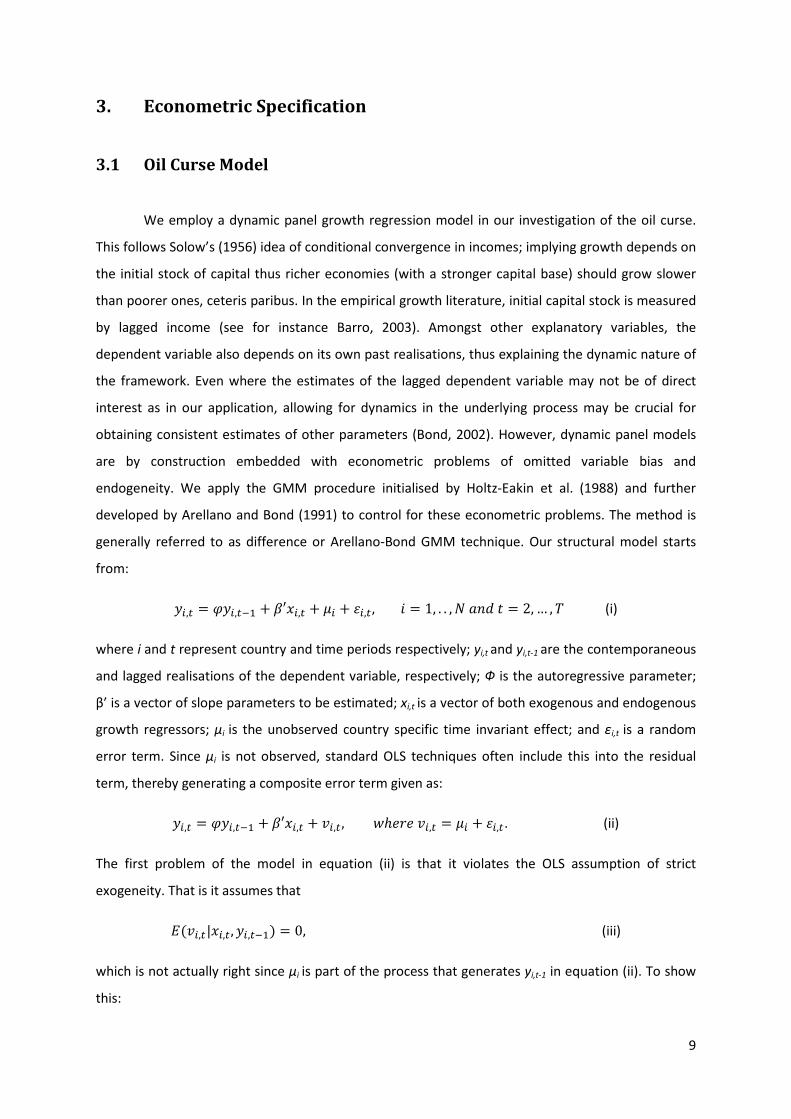
generally referred to as difference or Arellano-Bond GMM technique. Our structural model starts
from:
��,� = ���,��� + ′��,� + � + ��,�,� = 1, . . , ����� = 2,… , � (i)
where i and t represent country and time periods respectively; yi,t and yi,t-1 are the contemporaneous
and lagged realisations of the dependent variable, respectively; Ф is the autoregressive parameter;
β’ is a vector of slope parameters to be estimated; xi,t is a vector of both exogenous and endogenous
growth regressors; µi is the unobserved country specific time invariant effect; and εi,t is a random
error term. Since µi is not observed, standard OLS techniques often include this into the residual
term, thereby generating a composite error term given as:
��,� = ���,��� + ′��,� + ��,�,�ℎ�����,� = � + ��,�. (ii)
The first problem of the model in equation (ii) is that it violates the OLS assumption of strict
exogeneity. That is it assumes that
(��,�|��,�, ��,���) = 0, (iii)
which is not actually right since µi is part of the process that generates yi,t-1 in equation (ii). To show
this:
10
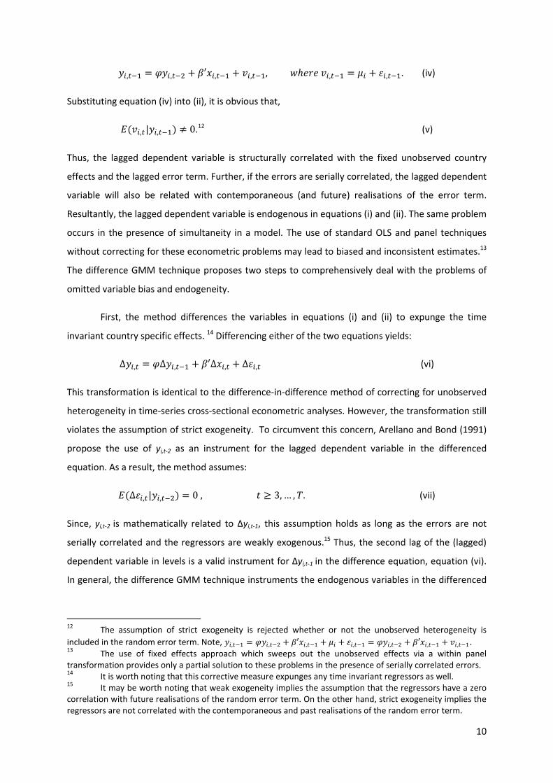
��,��� = ���,��% + ′��,��� + ��,���,�ℎ�����,��� = � + ��,���. (iv)
Substituting equation (iv) into (ii), it is obvious that,
(��,�|��,���) ≠ 0.12
(v)
Thus, the lagged dependent variable is structurally correlated with the fixed unobserved country
effects and the lagged error term. Further, if the errors are serially correlated, the lagged dependent
variable will also be related with contemporaneous (and future) realisations of the error term.
Resultantly, the lagged dependent variable is endogenous in equations (i) and (ii). The same problem
occurs in the presence of simultaneity in a model. The use of standard OLS and panel techniques
without correcting for these econometric problems may lead to biased and inconsistent estimates.13
The difference GMM technique proposes two steps to comprehensively deal with the problems of
omitted variable bias and endogeneity.
First, the method differences the variables in equations (i) and (ii) to expunge the time
invariant country specific effects. 14
Differencing either of the two equations yields:
∆��,� = �∆��,��� + ′∆��,� + ∆��,� (vi)
This transformation is identical to the difference-in-difference method of correcting for unobserved
heterogeneity in time-series cross-sectional econometric analyses. However, the transformation still
violates the assumption of strict exogeneity. To circumvent this concern, Arellano and Bond (1991)
propose the use of yi,t-2 as an instrument for the lagged dependent variable in the differenced
equation. As a result, the method assumes:
(∆��,�|��,��%) = 0,� ≥ 3,… , �. (vii)
Since, yi,t-2 is mathematically related to Δyi,t-1, this assumption holds as long as the errors are not
serially correlated and the regressors are weakly exogenous.15
Thus, the second lag of the (lagged)
dependent variable in levels is a valid instrument for Δyi,t-1 in the difference equation, equation (vi).
In general, the difference GMM technique instruments the endogenous variables in the differenced
12
The assumption of strict exogeneity is rejected whether or not the unobserved heterogeneity is
included in the random error term. Note, ��,��� = ���,��% + ′��,��� + � + ��,��� = ���,��% + ′��,��� + ��,���. 13
The use of fixed effects approach which sweeps out the unobserved effects via a within panel
transformation provides only a partial solution to these problems in the presence of serially correlated errors. 14
It is worth noting that this corrective measure expunges any time invariant regressors as well. 15
It may be worth noting that weak exogeneity implies the assumption that the regressors have a zero
correlation with future realisations of the random error term. On the other hand, strict exogeneity implies the
regressors are not correlated with the contemporaneous and past realisations of the random error term.
11
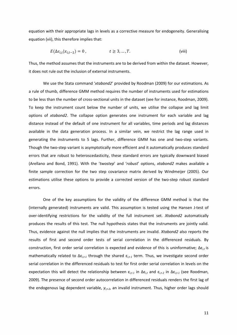
equation with their appropriate lags in levels as a corrective measure for endogeneity. Generalising
equation (vii), this therefore implies that:
(∆��,�|��,��%) = 0,� ≥ 3,… , �. (viii)
Thus, the method assumes that the instruments are to be derived from within the dataset. However,
it does not rule out the inclusion of external instruments.
We use the Stata command ‘xtabond2’ provided by Roodman (2009) for our estimations. As
a rule of thumb, difference GMM method requires the number of instruments used for estimations
to be less than the number of cross-sectional units in the dataset (see for instance, Roodman, 2009).
To keep the instrument count below the number of units, we utilise the collapse and lag limit
options of xtabond2. The collapse option generates one instrument for each variable and lag
distance instead of the default of one instrument for all variables, time periods and lag distances
available in the data generation process. In a similar vein, we restrict the lag range used in
generating the instruments to 5 lags. Further, difference GMM has one and two-step variants.
Though the two-step variant is asymptotically more efficient and it automatically produces standard
errors that are robust to heteroscedasticity, these standard errors are typically downward biased
(Arellano and Bond, 1991). With the ‘twostep’ and ‘robust’ options, xtabond2 makes available a
finite sample correction for the two step covariance matrix derived by Windmeijer (2005). Our
estimations utilise these options to provide a corrected version of the two-step robust standard
errors.
One of the key assumptions for the validity of the difference GMM method is that the
(internally generated) instruments are valid. This assumption is tested using the Hansen J-test of
over-identifying restrictions for the validity of the full instrument set. Xtabond2 automatically
produces the results of this test. The null hypothesis states that the instruments are jointly valid.
Thus, evidence against the null implies that the instruments are invalid. Xtabond2 also reports the
results of first and second order tests of serial correlation in the differenced residuals. By
construction, first order serial correlation is expected and evidence of this is uninformative; Δεi,t is
mathematically related to Δεi,t-1 through the shared εi,t-1 term. Thus, we investigate second order
serial correlation in the differenced residuals to test for first order serial correlation in levels on the
expectation this will detect the relationship between εi,t-1 in Δεi,t and εi,t-2 in Δεi,t-1 (see Roodman,
2009). The presence of second order autocorrelation in differenced residuals renders the first lag of
the endogenous lag dependent variable, yi,t-2, an invalid instrument. Thus, higher order lags should
12
be considered as instruments. A satisfaction of the Hansen and serial correlation diagnostic tests
gives credence to the adequacy of our instruments.
3.2 Explanatory Variables and Data Description
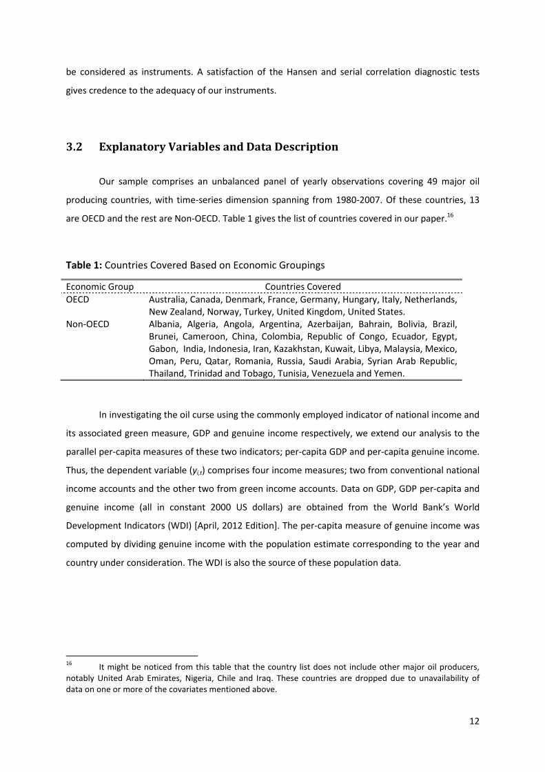
Our sample comprises an unbalanced panel of yearly observations covering 49 major oil
producing countries, with time-series dimension spanning from 1980-2007. Of these countries, 13
are OECD and the rest are Non-OECD. Table 1 gives the list of countries covered in our paper.16
Table 1: Countries Covered Based on Economic Groupings
Economic Group Countries Covered
OECD Australia, Canada, Denmark, France, Germany, Hungary, Italy, Netherlands,
New Zealand, Norway, Turkey, United Kingdom, United States.
Non-OECD Albania, Algeria, Angola, Argentina, Azerbaijan, Bahrain, Bolivia, Brazil,
Brunei, Cameroon, China, Colombia, Republic of Congo, Ecuador, Egypt,
Gabon, India, Indonesia, Iran, Kazakhstan, Kuwait, Libya, Malaysia, Mexico,
Oman, Peru, Qatar, Romania, Russia, Saudi Arabia, Syrian Arab Republic,
Thailand, Trinidad and Tobago, Tunisia, Venezuela and Yemen.
In investigating the oil curse using the commonly employed indicator of national income and
its associated green measure, GDP and genuine income respectively, we extend our analysis to the
parallel per-capita measures of these two indicators; per-capita GDP and per-capita genuine income.
Thus, the dependent variable (yi,t) comprises four income measures; two from conventional national
income accounts and the other two from green income accounts. Data on GDP, GDP per-capita and
genuine income (all in constant 2000 US dollars) are obtained from the World Bank’s World
Development Indicators (WDI) [April, 2012 Edition]. The per-capita measure of genuine income was
computed by dividing genuine income with the population estimate corresponding to the year and
country under consideration. The WDI is also the source of these population data.
16
It might be noticed from this table that the country list does not include other major oil producers,
notably United Arab Emirates, Nigeria, Chile and Iraq. These countries are dropped due to unavailability of
data on one or more of the covariates mentioned above.
13
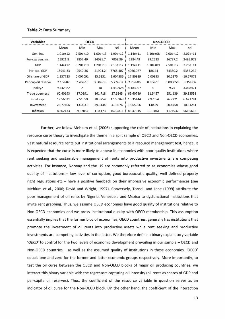
Table 2: Data Summary
Variables OECD Non-OECD
Mean Min Max sd Mean Min Max sd
Gen. inc. 1.01e+12 2.50e+10 1.00e+13 1.90e+12 1.14e+11 3.10e+08 2.00e+12 2.07e+11
Per-cap gen. inc. 15921.8 2857.49 34081.7 7009.39 2284.49 99.2533 16737.2 2495.973
GDP 1.14e+12 3.20e+10 1.20e+13 2.13e+12 1.19e+11 1.70e+09 2.50e+12 2.26e+11
Per-cap. GDP 18941.33 2540.36 41904.2 8768.407 4066.077 186.44 34380.2 5355.232
Oil share of GDP 1.357723 0.007091 15.6331 2.604386 17.80939 0.00893 80.2375 16.67073
Per-cap oil reserve 2.16e-07 7.20e-10 3.50e-06 5.77e-07 2.79e-06 8.80e-10 0.000059 8.35e-06
ipolity2 9.442982 2 10 1.439928 4.183007 0 9.75 3.028421
Trade openness 60.40693 17.0891 161.718 27.6245 69.60739 11.5457 251.139 39.83551
Govt exp. 19.56031 7.51559 28.3754 4.155963 15.35444 2.97554 76.2221 6.621791
Investment 25.77406 13.0931 39.3144 4.13076 18.65066 1.8459 60.4758 10.51251
Inflation 8.862133 -9.62854 110.173 16.32811 85.47915 -11.6861 11749.6 561.5613
Further, we follow Mehlum et al. (2006) supporting the role of institutions in explaining the
resource curse theory to investigate the theme in a split sample of OECD and Non-OECD economies.
Vast natural resource rents put institutional arrangements to a resource management test, hence, it
is expected that the curse is more likely to appear in economies with poor quality institutions where
rent seeking and sustainable management of rents into productive investments are competing
activities. For instance, Norway and the US are commonly referred to as economies whose good
quality of institutions – low level of corruption, good bureaucratic quality, well defined property
right regulations etc – have a positive feedback on their impressive economic performances (see
Mehlum et al., 2006; David and Wright, 1997). Conversely, Tornell and Lane (1999) attribute the
poor management of oil rents by Nigeria, Venezuela and Mexico to dysfunctional institutions that
invite rent grabbing. Thus, we assume OECD economies have good quality of institutions relative to
Non-OECD economies and we proxy institutional quality with OECD membership. This assumption
essentially implies that the former bloc of economies, OECD countries, generally has institutions that
promote the investment of oil rents into productive assets while rent seeking and productive
investments are competing activities in the latter. We therefore define a binary explanatory variable
’OECD’ to control for the two levels of economic development prevailing in our sample – OECD and
Non-OECD countries – as well as the assumed quality of institutions in these economies. ‘OECD’
equals one and zero for the former and latter economic groups respectively. More importantly, to
test the oil curse between the OECD and Non-OECD blocks of major oil producing countries, we
interact this binary variable with the regressors capturing oil intensity (oil rents as shares of GDP and
per-capita oil reserves). Thus, the coefficient of the resource variable in question serves as an
indicator of oil curse for the Non-OECD block. On the other hand, the coefficient of the interaction
14
term gives the slope differential of the curse between the two groups.17
Data on resource rents as
shares of GDP and proved crude oil reserves (in billion barrels) are obtained from the World Bank’s
WDI and US Energy Information Administration, respectively. The per-capita measure of oil reserves
is obtained by dividing the total reserves by the population figures obtained from the World Bank’s
WDI (April, 2012 Edition).18
Consistent with the growth literature, other controls include trade openness defined as sum
of imports and exports as a percentage of GDP; government expenditure (a proxy for government
size and distortions in the economy) defined as general government final consumption expenditure
as a percentage of GDP; investment defined as domestic investments as a percentage of GDP;
inflation rate (to capture macroeconomic instability) defined as inflation in consumer prices (annual
percentage); and a democracy index ‘ipolity2’ ranging from 0 to 10, with lower and higher values
indicating least and most democratic economies respectively (see for instance, Bjorvatn et al., 2012;
Brunnschweiler and Bulte, 2008; Carbonnier and Wagner, 2011). Investment and ipolity2 are
obtained from the University of Gothenburg Quality of Government Standard Dataset available at
http://www.qog.pol.gu.se/data/. The other variables are obtained from the World Bank’s WDI (April,
2012 Edition). Hence, in addition to the lagged dependent variable arising from the dynamic nature
of our data generation process, our set of covariates includes the two key variables measuring oil
intensity – oil rents as shares of GDP and per-capita oil reserves, – the OECD binary variable and its
interactions with the resource variables, ipolity2, trade openness, government expenditure,
investment and inflation rate. We treat all of these variables as endogenous. Thus, we generate
instruments for them as standard in the Arellano-Bond GMM method using all their available lags for
each time period in levels (see Roodman, 2009). However, we restrict the lag-range to 5 lags to avoid
instrument proliferation as previously alluded to.19
All of the variables used for the estimations (both right and left hand side) are measured in
logs, with the exception of inflation rate. Table 2 provides summary statistics for the variables
17
It is worth noting that the difference transformation adopted by the difference GMM procedure, as
explained in equation (vi), sweeps out the OECD binary variable (in level) as it is time invariant. However, the
time varying interaction term remains. We are particularly interested in the coefficient of the interaction term
capturing the curse differential between the OECD and Non-OECD economies instead of the coefficient of the
OECD binary variable merely capturing the difference in intercepts between the two groups. The latter
coefficient might be important if the model was meant for predictive reasons but this is not the case in this
paper. 18
Oil reserves data are obtained from http://www.eia.gov/. 19
Virtually all the covariates have a GDP or population metric. Thus, it is very probable that there is bi-
directional causality between each of the control variables and the dependent variables. This informs our
choice for treating all the right hand side variables as endogenous. Even if any of the variables was exogenous,
there should not be any bias arising from this assumption as long as the instruments applied for these
variables are related to the variables they stand for and they satisfy the diagnostic tests.
15
employed for the paper’s estimations, separated by the two economic groups covered. The table
presents the mean, standard deviation (sd), minimum and maximum values of the variables. From
the table, it is not surprising that the OECD group has a relatively higher mean genuine income and
GDP estimates (in both aggregate and per-capita terms) than the Non-OECD group. Conversely, the
OECD bloc has a relatively lower mean estimate of oil rents as a share of GDP than the Non-OECD
bloc; 1.36 percent compared to 17.81 percent for the former and latter, respectively. Also, the Non-
OECD group has a much higher mean per-capita oil reserve estimate than its OECD counterparts –
2,790 barrels compared to 216 barrels.20
Further, the OECD bloc has a remarkably higher degree of
democratisation and macroeconomic stability (measured by the mean values of ipolity2 and
inflation) than the Non-OECD bloc. In fact, the latter bloc has a below average democratisation score
and a very high macroeconomic instability.
20
Note crude oil reserves are measured in billion barrels.
16
Table 3: Results of Arellano-Bond Two-step Dynamic Panel GMM Estimations (Windmeijer’s Robust and Corrected Standard Errors in
Parenthesis)
NB: AR(1) and AR(2) test p-values are the reported p-values for the first and second order tests of serial correlation in the differenced residuals.
*, ** and *** denote significance at the one, five and ten percent levels respectively.
Dependent Variables
ln(GDP) ln(Gen Inc.) ln(GDP) ln(Gen. Inc.) ln(GDP Per-cap) ln(Gen. Inc. Per-cap) ln(GDP Per-cap) ln(Gen. Inc. Per-cap)
[1a] [1b] [2a] [2b] [3a] [3b] [4a] [4b]
Explanatory Variables:
lagged dependent variable 1.0178*
(0.0297)
0.9993*
(0.0763)
1.0232*
(0.0331)
0.9752*
(0.0546)
1.0018*
(0.0435)
0.9140*
(0.0927)
0.9868*
(0.0506)
0.9561*
(0.0995)
ln(oil share of GDP) -0.0071
(0.0217)
-0.0734**
(0.0336)
– – -0.0119
(0.0239)
-0.0864**
(0.0407)
– –
ln(oil share of GDP) *OECD 0.0142
(0.0240)
0.0968**
(0.0427)
– – 0.0137
(0.0263)
0.0936**
(0.0467)
– –
ln(per-capita oil reserves) – – -0.0269
(0.0447)
-0.1540**
(0.0815)
– – -0.0441
(0.0390)
-0.2024***
(0.1030)
ln(per-capita oil reserves) *OECD – – 0.0617
(0.0571)
0.2112**
(0.1010)
– – 0.0755
(0.0506)
0.2766***
(0.1531)
ln(ipolity2) 0.0009
(0.0364)
0.0126
(0.0685)
-0.0025
(0.0319)
0.0386
(0.0633)
0.0016
(0.0398)
0.0349
(0.0620)
0.0093
(0.0242)
0.0402
(0.0588)
ln(trade openness) 0.0012
(0.0374)
0.0051
(0.1115)
0.0157
(0.0478)
0.0685
(0.0695)
0.0285
(0.0452)
0.1005
(0.1049)
0.0658
(0.0445)
0.0889
(0.0796)
ln(govt. exp. as shares of GDP) -0.0870***
(0.0507)
-0.1876*
(0.0514)
-0.1027*
(0.0323)
-0.1608*
(0.0525)
-0.1261*
(0.0420)
-0.1739*
(0.0630)
-0.0786***
(0.0406)
-0.1361**
(0.0609)
ln(investment as shares of GDP) 0.0613**
(0.0270)
0.2245*
(0.0450)
0.0463
(0.0300)
0.1967*
(0.0558)
0.0624**
(0.0273)
0.2361*
(0.0442)
0.0531**
(0.0254)
0.2200*
(0.0552)
inflation -0.000021**
(0.000011)
-5.62e-06
(8.90e-06)
-0.000016**
(7.79e-06)
-7.38e-06
(9.12e-06)
-0.000021***
(0.000011)
-3.42e-06
(8.99e-06)
-0.000016**
(7.53e-06)
-6.60e-06
(9.06e-06)
No. of Obs 982 890 963 872 979 890 962 872
No. of Groups 49 44 49 44 49 44 49 44
No. of Instruments 40 40 40 40 40 40 40 40
AR(1) Test P-Value 0.000 0.007 0.000 0.002 0.000 0.008 0.000 0.003
AR(2) Test P-Value 0.373 0.306 0.280 0.689 0.285 0.329 0.397 0.805
Hansen P-Value 0.194 0.186 0.111 0.364 0.151 0.200 0.187 0.439
17
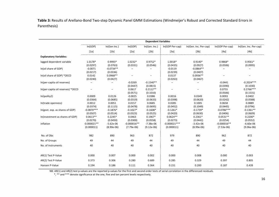
4. Results and Discussions
Table 3 presents the results of the Arellano-Bond difference GMM estimations. The table is
divided into two sections. The first section employs the aggregate measures of GDP and genuine
income as its left hand side variables. Then, the alternating pair of columns labelled ‘a’ and ‘b’
denote the use of GDP and genuine income as the dependent variables, respectively. Also, the first
and last sets of columns in this section, ‘[1a] and [1b]’ and ‘[2a] and [2b]’, employ oil rents as shares
of GDP and per-capita oil reserves as their measures of oil intensity respectively. The second section
of the table presents an analogous representation of the results using the per-capita measures of
GDP and genuine income as its dependent variables. In the table, the prefix before variable names
“ln” indicates natural log of the variables. Further, the bottom of the table presents: (a) the number
of observations, groups and instruments used in the estimation of all models ([1a], [1b],…,[ 4b]); (b)
the p-values for the first and second order tests of serial correlation in the differenced residuals; (c)
the Hansen test of over-identifying restrictions examining the joint validity of instruments.
Concentrating on the most important variables to our investigation, the results in the first
section of the table employing the aggregate measures of GDP and genuine income as its
regressands (models [1a], [1b], [2a], and [2b]) show evidence of an inverse relationship between
income and the resource variables irrespective of the indicator of oil intensity considered. Foremost,
the coefficients of oil share of GDP and per-capita oil reserve variables in models [1a] and [2a] show
that a ten percent increase in oil intensity of the Non-OECD bloc leads to a 0.07 percent and 0.27
percent decrease in GDP, respectively. Analogously, the results in [1b] and [2b] show that a ten
percent increase in oil rents as a share of GDP and per-capita oil reserves leads to a 0.73 percent and
1.54 percent decrease in genuine income of the Non-OECD group, respectively. These findings
therefore suggest an existence of the curse in the Non-OECD bloc of oil producing economies. Also,
the results indicate that the curse may be stronger for the genuine income measure of sustainable
economic progress relative to the GDP indicator. However, it is worth noting that our finding of a
negative association between oil intensity and income whilst employing the GDP indicator is not
backed by statistical tests of significance, thus, making the curse somewhat inconclusive for this
standard measure of income. Nevertheless, an appraisal of the results arising from the use of the
genuine income measure for the estimations still indicates that the Non-OECD oil producing
countries have not been successful in investing their oil rents in other forms of capital. Conversely,
oil resources are a blessing to the OECD oil producing countries. The coefficients of the variables
capturing the oil curse differential between the OECD and Non-OECD groups (that is, the interaction
18
terms between oil intensity variables and OECD binary variable) are positive and they offset the
negative slope for the Non-OECD group. In particular, the significant interaction terms given by
models [1b] and [2b] show that a ten percent increase in oil share of GDP and per-capita oil reserves
leads to a 0.23 percent and 0.57 percent increase in the genuine incomes of the OECD bloc,
respectively.21
The resource and interaction variables in these models – [1b] and [2b] – are jointly
significant at the five and ten percent levels respectively. Thus, the OECD bloc experiences an ‘oil
blessing’ using genuine income measures in appraising their management of oil rents. These
countries may be classified as sustainable as they have satisfied the Hartwick rule whilst extracting
their oil resources.
Similar results are obtained in the second section of the table employing the per-capita
measures of GDP and genuine income as its left hand side variables. Again, the negative correlation
between oil intensity and income is validated for both measures of income. Models [3a] and [4a]
indicate that a ten percent increase in oil rents as a share of GDP and per-capita oil reserves is
associated with a 0.12 and 0.44 percent fall in per-capita GDP of the Non-OECD oil exporting
countries, respectively. The corresponding models employing green measures of per-capita income
show that a ten percent increase in oil share of GDP and per-capita oil reserves leads to a 0.86 and
2.02 percent decrease in per-capita genuine income of the Non-OECD group, respectively. Once
more, it may seem that this negative association is stronger for per-capita measure of genuine
income relative to per-capita GDP indicator but we refrain from making such a conclusion as the
results for the latter indicator of income are not statistically significant. Thus, as in aggregate
genuine income, the oil curse is confirmed in per-capita genuine income also. Conversely, oil rents is
reconfirmed to be a blessing to the OECD bloc employing the per-capita measure of genuine income
in evaluating their adherence to the Hartwick rule. The interaction terms in models [3b] and [4b]
indicate that a ten percent increase in oil rents as shares of GDP and per-capita oil reserves leads to
a 0.07 percent and 0.74 percent rise in the per-capita genuine incomes of the OECD bloc,
respectively. Also, an F-test of joint significance indicates that the resource and interaction variables
in model [3b] are jointly significant at the ten percent level. In model [4b], a joint test on the
resource and interaction variables confirms they are marginally insignificant at the ten percent level
but the two variables are individually significant at the ten percent level.
Our confirmation of the oil curse in genuine income but not GDP indicators of economic
output is in line with earlier studies that have explored the natural resource curse theory. Mickesell
21
The marginal effects of these two indicators of resource intensity for the OECD bloc are obtained by
summing the slope of the resource variable under consideration with the slope of its corresponding interaction
term.
19
(1997) suggested that if GDP was adjusted for natural capital depreciation, the curse would be
stronger in adjusted income. Also, we explored suggestions in the literature review section of the
paper that Ecuador, Nigeria and Venezuela may be suffering from the oil curse as these economies
dissipate a good proportion of their oil rents on boosting consumption through various subsidy and
tax reduction policies (see Kellenberg, 1996; Hamilton et al., 2006). In line with these suggestions,
Atkinson and Hamilton (2003) recommend a shift from the dissipation of resource rents for financing
current consumption to prudent investments in man-made capital as one of the avenues of avoiding
the curse. This recommendation conforms to the Hartwick rule for sustainable management of
natural resource rents. Thus, our paper provides additional evidence to the suggestion that if the
unsustainable component of income was adjusted for natural capital depreciation, then the oil curse
in genuine income may be stronger than the curse in GDP in the presence of a significant evidence of
the curse in the latter. A reliance on our finding of a statistically insignificant negative association
between GDP and oil intensity may generate suggestions that the curse may not be a serious
resource management issue that requires concerted effort for the implementation of policies aimed
at achieving sustainable resource management. On the other hand, our finding of the curse in
adjusted measures of income indicates the gravity of natural resource mis-management in Non-
OECD economies thereby providing signals for the need of appropriate measures to sustainably
manage natural resource rents in these economies.
A further appraisal of the results in table 3 leads to two important findings. First, the curse is
stronger for the per-capita measure of genuine income relative to the aggregate indicator given a
measure of resource intensity used in the investigations. For instance, a comparison of models [1b]
and [3b] employing oil share of GDP as their measure of oil intensity shows the curse to be weaker in
the former model using an aggregate measure of genuine income as its dependent variable; the
resource variable turns up an impairing elasticity of 0.07 percent in [1b] compared to 0.09 percent in
[3b]. A comparison of [2b] and [4b] amounts to the same finding using per-capita oil reserves as the
measure of oil intensity.22
Speculatively, this result may be an indication that the relatively high
population growth rates usually recorded by developing countries might be an obstacle to their
sustainable development. And as such, it suggests that population control measures may be an
avenue of achieving sustainability in these countries. Second, we find the curse to be stronger for
per-capita oil reserves measure of oil intensity relative to share of oil rents in GDP given an indicator
of genuine income employed for the exploration. For example, a comparison of the elasticities of oil
rents as shares of GDP in model [1b] and per-capita oil reserves in [2b] shows the former model to
22
This also applies to the aggregate and per-capita measures of GDP but we do not pay much attention
to this given that the ascertained growth impairing effects of resource intensity are not significant.
20
have a weaker impairing effect on genuine income than the latter; 0.07 percent in [1b] compared to
0.15 percent in [2b]. The same finding applies to a comparison of [3b] and [4b] employing per-capita
genuine income as their outcome variable.23
Despite the estimates of the lagged dependent variable not being particularly important to
our investigations, these autoregressive parameters are significant and approximately 1.0 in all
models. This implies the outcome variables (aggregate and per-capita measures of GDP and genuine
income) are highly persistent with a high predictive power; essentially, the contemporaneous values
of the dependent variables are highly dependent on their past realisations, thus, justifying the
adoption of a dynamic framework in our analyses. Additionally, we find government expenditure as
shares of GDP and inflation to exert a negative effect on both aggregate and per-capita measures of
GDP and genuine income while investment as shares of GDP exerts a positive effect on the outcome
variables. These findings are consistent with the following: Barro (1991), Bjorvatn et al. (2012) and
Afonso and Furceri (2010) find that government size exerts a negative effect on growth,24
and,
Neumayer (2004) and Bjorvatn et al. (2012) find investment to exert a positive effect on growth. The
other regressors capturing the degree of democratisation and trade openness generally turn up a
positive effect on the outcome variables but this relationship is not significant.
Finally, the results in the bottom of the table indicate that our estimations satisfy the
specification tests of the Arellano-Bond difference GMM method. First, the number of instruments is
less than the number of groups in all models. Second, as it is expected, the p-values of AR(1) indicate
the presence of first order serial correlation in the differenced residuals. However, the AR(2) p-
values reject this serial correlation for the second order form. Thus, the residuals in the levels
equation are not serially correlated. Thirdly, the Hansen test of joint validity of instruments fails to
23
It is worth noting that our investigation of the curse employs the levels but not the growth rates of
the dependent variables. However, employing the growth rates of the variables only affects the magnitudes of
the effects of the explanatory variables and the major findings of the paper remain unchanged. Essentially, the
following results remain unchanged using the growth rates of the variables: there is still inconclusive evidence
of the curse in GDP and per-capita GDP as the negative slopes of the resource variables are not significant; the
oil curse and blessing in aggregate and per-capita genuine income is still confirmed for Non-OECD and OECD
economies respectively; the curse is stronger in per-capita relative to aggregate genuine income; and the curse
is stronger in per-capita oil reserves relative to share of oil rents in GDP. 24
It is worth noting that there is no consensus on the effect of government size on growth in the
development economics literature. Inasmuch as there are ‘negative proponents’ of this effect, there are
‘positive proponents’ as well. The former argue that a larger government size crowds out private investment
and leads to economic inefficiencies thereby inhibiting growth. However, we do not delve much on this debate
in this paper given that government size is not one of our major variables of interest.
21
reject the null hypothesis that the set of instruments employed for the estimations are valid. Thus,
the instruments generated are adequate for the estimations.25
5. Concluding Remarks
The conception of the resource curse theory generated a considerable change in the
classical reasoning that vast natural resource endowments serve as a driver for economic progress.
Instead, the theory prescribed a paradoxical role for natural resource abundance; economies with
vast natural resource endowments, particularly exhaustible resources, often record lower growth
rates than resource scarce economies. Obviously, this is not an all-embracing theory as there are a
few exempt countries that have successfully converted their natural resource rents into considerable
levels of economic development. Norway and Botswana are prime examples of countries that have
successfully converted their oil and diamond rents into remarkable levels of economic progress.
Contrary to the paradoxical term ‘resource curse’, these countries experience a ‘resource blessing’.
On the other hand, Venezuela and Nigeria are often cited as prime victims of the oil curse. These
countries have been unable to satisfy the Hartwick rule in managing their oil rents.
Existing studies investigating the curse mostly employ cross-country and panel growth
regressions for their analyses. As these techniques are subject to endogeneity concerns, the use of
alternative methods that correct these problems is needed. Also, a significant amount of these
studies regress an income measure, GDP in its aggregate or per-capita terms, on a measure of
resource intensity (particularly the share of natural resource rents in GDP) and other factors that are
thought to affect economic growth. However, the use of standard GDP measures for investigating
the curse does not depict the true incomes of resource intensive economies. Traditional national
income accounts records rents from natural resource extraction as a positive contribution to income
without making a corresponding correction for the value of depleted natural resource stock. This
system of national accounts is inconsistent with green accounting practices and it leads to a positive
bias in the national income computations of resource intensive economies. Thus, this shortcoming of
25
It is worth mentioning that this test marginally rejects the null at the ten percent level in model [2a].
Extending the restricted lag limits for this model from five to six lags turns up a Hansen p-value of 0.223. This
brings the instrument count to 48, which is still below the number of groups, 49. At the same time, the
coefficients in the model remain largely unchanged but the investment variable now becomes significant at
the ten percent level.
22
standard income measures requires the application of greener and more sustainable measures of
national income in resource curse explorations.
We employ the Arellano-Bond dynamic panel difference GMM method to control for
endogeneity in our investigations of the oil curse in major OECD and Non-OECD oil producing
economies. In addition to investigating the curse in standard income measures (GDP and per-capita
GDP), we explore the curse in genuine income measures as well. Also, our investigation employs two
competing measures of resource intensity: share of oil rents in GDP and per-capita oil reserves. We
confirm the oil curse in Non-OECD countries employing both aggregate and per-capita measures of
genuine income. However, the curse is stronger in the per-capita measure of genuine income. Given
that aggregate genuine income is scaled by population estimates to arrive at its corresponding per-
capita measure, this finding generates a speculation that the relatively high population growth rates
usually recorded by developing countries may be a medium through which resource abundance
translates to lower economic progress. Further, we find the curse to be stronger for the per-capita
oil reserves measure of oil intensity. Again, this reiterates the speculation of high population growth
rates in oil rich Non-OECD countries to be growth impairing. There is considerable evidence in the
literature that resource intensive countries have been unable to escape the curse due to the
conspicuous consumption pattern, high corruption and rent seeking associated with vast natural
resource endowments. Thus, a good blend of sound investment decisions (to satisfy the Hartwick
rule), population control and anti-corruption measures by the Non-OECD countries should generate
impetus for escaping the curse. Though we find a negative association between oil intensity and GDP
measures of economic performance, this correlation remains inconclusive as the results are not
statistically significant. Conversely, we find the two measures of oil intensity considered (share oil
rents in GDP and per-capita oil reserves) to exert a positive effect on the genuine incomes of OECD
oil producing economies. Thus, the OECD countries experience an ‘oil blessing’ and they may be
classified as sustainable based on the management of their oil rents.
This paper is restrictive in its coverage of natural resources in the investigations. Though our
focus on oil is dictated by an objective to explore the oil curse, future studies could investigate the
curse for other mineral, agricultural or forest resources. Also, the analysis could be extended by
employing the genuine savings (and probably other green measures of income) for the
investigations. Another important area of further research is the likely mechanisms explaining the
curse, especially the role of political and bureaucratic factors (level of corruption, rule of law, quality
of institutions, property rights enforcement etc). A deeper insight into these mechanisms could
provide a basis for recommending the most important policies needed to escape the curse.
23
References
Afonso, A. and Furceri, D. (2010). “Government Size, Composition, Volatility and Economic Growth.”
European Journal of Political Economy 26(4): 517-532.
Alexeev, M. and Conrad, R. (2009). “The Elusive Curse of Oil.” The Review of Economics and
Statistics, 91(3): 586-598.
Arrellano, M. and Bond, S. (1991). “Some Tests of Specification for Panel Data: Monte Carlo Evidence
and an Application to Employment Equations.” Review of Economic Studies, 58(2): 277-297.
Arrow, K.; Dasgupta, P.; Goulder, L.; Daily, G.; Ehrlich, P.; Heal, G.; Levin, S.; Maler, K.; Schneider, S.;
Starrett, D. and Walker, B. (2004) “Are We Consuming too Much?” Journal of Economic
Perspectives, 18(3): 147-172.
Arrow, K.; Dasgupta, P.; Goulder, L.; Mumford, K. and Oleson, K. (2012). “Sustainability and the
Measurement of Wealth.” Environment and Development Economics, 17(3): 317-353.
Atkinson, G. and Hamilton, K. (2003). “Savings, Growth and the Resource Curse Hypothesis.” World
Development, 31(11)1793-1807.
Barbier, E. (2010). “Corruption and the Political Economy of Resource-Based Development: A
Comparison of Asia and sub-Saharan Africa.” Environmental and Resource Economics,
46(4):511-537
Barro, O. (1991). “Economic Growth in a Cross Section of Countries.” Quaterly Journal of Economics,
106(2):407-443.
Barro, R. (2003). “Determinants of Economic Growth in a Panel of Countries.” Analysis of Economics
and Finance, 4():231-274
Barro, R. and Sala-i-Martin, X. (1995). Economic Growth. McGraw Hill, New York.
Bjorvatn, K.; Farzanegan, M. and Schneider, F. (2012). “Resource Curse and Power Balance: Evidence
from Oil-Rich Countries.” World Development, 40(7): 1308-1316.
Bond, Stephen. (2002). Dynamic Panel Data Models: A Guide to Micro Data Methods and Practice.
The Institute for Fiscal Studies, Department of Economics, UCL. Cemmap Working Paper
CWP09/02
Boos, A. and Holm-Muller, K. (2012) “A Theoretical Review of the Relationship between the
Resource Curse and Genuine Savings as an Indicator of ‘Weak’ Sustainability.” Natural
Resources Forum, 36:145-159.
Brunnschweiler, C. and Bulte, E. (2008). “The Resource Curse Revisited: A Tale of Paradoxes and Red
Herrings.” Journal of Environmental Economics and Management, 55:248-264.
Carbonnier, G.; Wagner, N. and Brugger, F. (2011). Oil, Gas and Minerals: The Impact of Resource-
Dependence and Governance on Sustainable Development. The Center on Conflict,
24
Development and Peacebuilding (CCDP) Working Paper. Available at
http://graduateinstitute.ch/webdav/site/ccdp/shared/6305/Working_Paper_8_Web%20versi
on%202.pdf
David, P., and Wright, G. (1997). “Increasing Returns and the Genesis of American Resource
Abundance.” Industrial and Corporate Change, 6(2): 233-245.
Dietz, S.; Neumayer, E. and De Soysa, I. (2007). “Corruption, the Resource Curse and Genuine
Savings.” Environment and Development Economics, 12(1):33-53.
Frankel, J. (2010). The Natural Resource Curse: A Survey. NBER Working Paper No. 15836. Available
online at http://www.nber.org/papers/w15836
Hamilton, K. and Clemens, M. (1999). “Genuine Savings Rates in Developing Countries.” The World
Bank Economic Review, 12(2): 333-356.
Hamilton, K.; Ruta, G. and Tajibaeva, L. (2006). “Capital Accumulation and Resource Depletion: A
Hartwick Rule Counterfactual.” Environmental and Resource Economics, 34(4): 517-533.
Hartwick, M. (1977). “Intergenerational Equity and the Investing of Rents from Exhaustible
Resources.” American Economic Review, 67(5): 972-974.
Hartwick, M. (2009). “What Would Solow Say?” Journal of Natural Resource Policy Research, 1(1):
91-96
Holtz-Eakin, D.; Newey, W. and Rosen, S. (1988). “Estimating Vector Autoregressions with Panel
Data.” Econometrica, 56(6): 1371-1395
Kellenberg, J. (1996) Accounting for Natural Resources in Ecuador; Contrasting Methodologies,
Conflicting Results. Washington D.C, World Bank.
Mehlum, H.; Moene, K. and Torvik, R. (2006). “Institutions and the Resource Curse.” The Economic
Journal, 116(508): 1-20.
Mickesell, F. (1997). “Explaining the Resource Curse, with Special Reference to Mineral-Exporting
Countries.” In: Neumayer, E. (2004). “Does the ‘Resource Curse’ Hold for Growth in Genuine
Income as Well?” World Development, 32(10): 1627-1640.
Neumayer, E. (2004). “Does the ‘Resource Curse’ Hold for Growth in Genuine Income as
Well.” World Development, 32(10): 1627-1640.
Roodman, David. (2009) “How to do Xtabond2: An Introduction to Difference and System GMM in
Stata.” Stata Journal, 9(1): 86-136.
Papyrakis, E. and Gerlagh, R. (2004) “The Resource Curse Hypothesis and its Transmission Channels.”
Journal of Comparative Economics, 32(1):181-193.
Sachs, J. and Warner, A. (1995). Natural Resource Abundance and Economic Growth. NBER Working
Paper, No. 5398.
25
Sala-i-Martin, X. and Subramanian, A. (2003). Addressing the Natural Resource: An Illustration from
Nigeria. NBER Working Paper, No. 9804.
Solow, R. (1956). “A Contribution to the theory of Economic Growth.” Quarterly Journal of
Economics, 70(1): 65-94.
Solow, R. (1986). “On the Intergenerational Allocation of Natural Resources.” Scandinavian Journal
of Economics, 88(1): 141-149.
Solow, R. (1992). “Sustainability; An Economists Perspective” in Stavins, R. (2005). Economics of the
Environment – Selected Readings. W. W. New York, NY, Norton and Company.
Tornell, A. and Lane, P. (1999). “The Voracity Effect.” American Economic Review, 89(1): 22-46.
Windmeijer, F. (2005). “A Finite Sample Correction for the Variance of Linear Efficient Two-step
GMM Estimators.” Journal of Econometrics, 126(1):25-51.
Wooldridge, J. (2008). Introductory Econometrics: A Modern Approach. Thomson, South-Western.
World Bank. (1997). Expanding the Measure of Wealth. The World Bank, Washington, D.C.
World Bank. (2011). The Changing Wealth of Nations. Measuring Sustainable Development in the
New Millenium. The World Bank, Washington, D.C.
World Bank (2012). World Development Indicators, April 2012 Edition. Available via
http://web.worldbank.org/