An Investigation of Atmospheric Mercury Deposition

to Bay Area Storm Runoff: a Pilot Study

Sarah Rothenberg, Lester McKee, Don Yee, Alicia Gilbreath, Michelle Lent

February 20, 2008

1. Introduction to atmospheric mercury

2. Methods

3. ResultsA. Dry deposition ratesB. Wet deposition rates

4. Summary

Overview of presentation

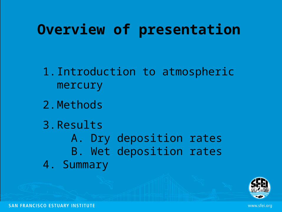
Atmospheric Mercury (Hg)

1. Sources (Mason et al., 1994)

Anthropogenic (80%)

Natural (20%)

2. Speciation and Residence Time (Lindberg et al., 2007)

Gaseous Elemental Hg (Hgo): ~ 1 year

Reactive Gaseous Hg (RGM): minutes-weeks

Particulate Hg (Hgp): minutes-weeks

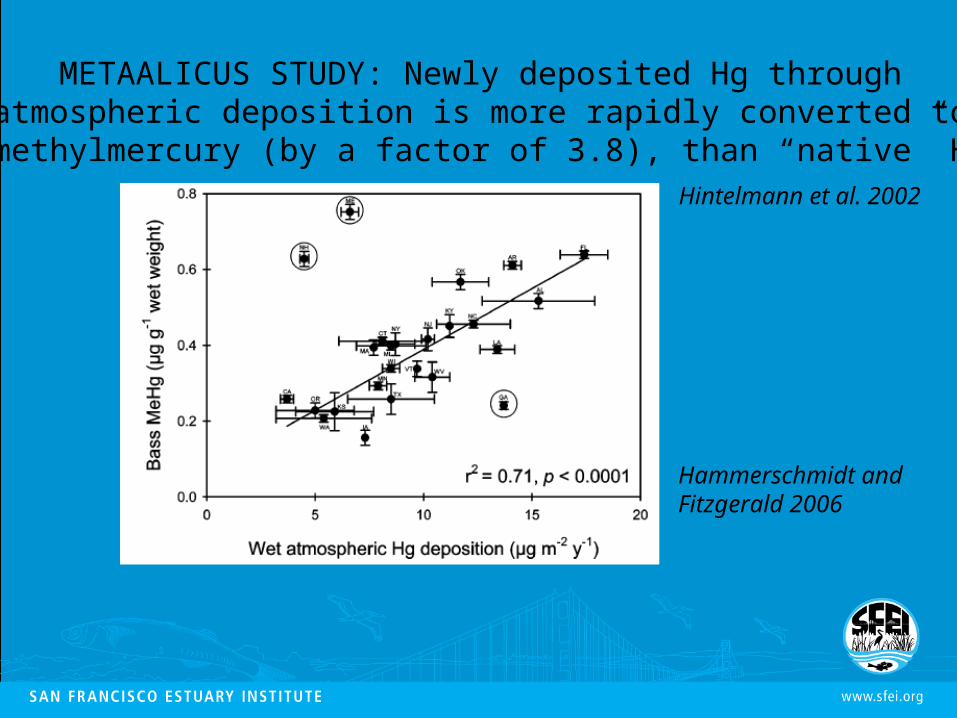
Hintelmann et al. 2002

METAALICUS STUDY: Newly deposited Hg through atmospheric deposition is more rapidly converted to methylmercury (by a factor of 3.8), than “native” Hg

Hammerschmidt and Fitzgerald 2006

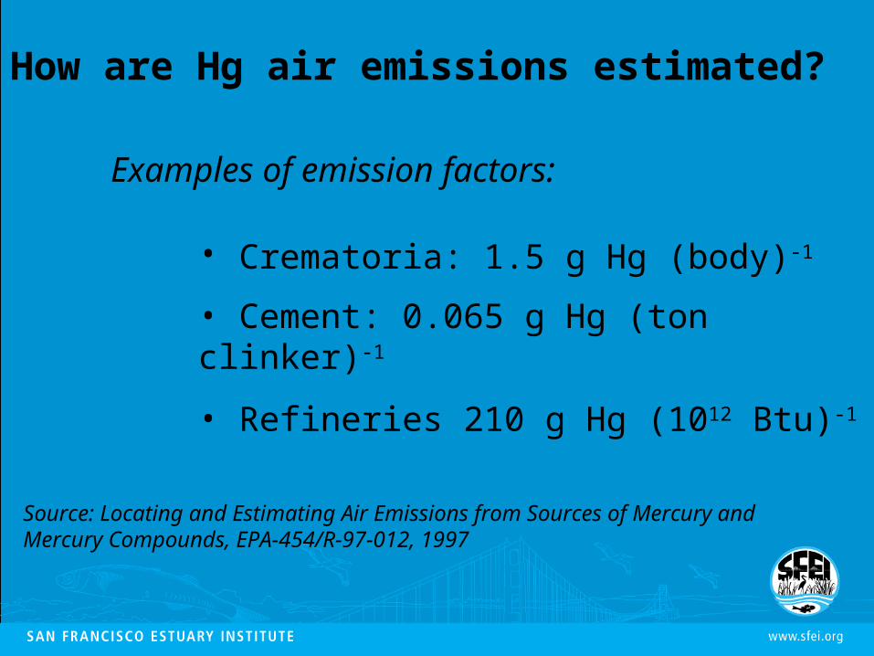
Examples of emission factors:

• Crematoria: 1.5 g Hg (body)-1

• Cement: 0.065 g Hg (ton clinker)-1

• Refineries 210 g Hg (1012 Btu)-1

Source: Locating and Estimating Air Emissions from Sources of Mercury and Mercury Compounds, EPA-454/R-97-012, 1997

How are Hg air emissions estimated?

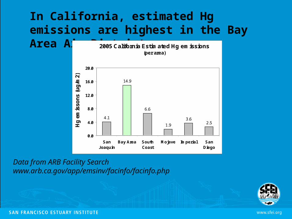
In California, estimated Hg emissions are highest in the Bay Area Air District.

Data from ARB Facility Searchwww.arb.ca.gov/app/emsinv/facinfo/facinfo.php

2005 California Estimated Hg emissions (per area)

4.1

14.9

6.6

1.9

3.62.5

0.0

4.0

8.0

12.0

16.0

20.0

SanJoaquin

Bay Area SouthCoast

Mojave Imperial SanDiego

Hg

em

isso

ns

(ug

/m2)

Data from ARB Facility Searchwww.arb.ca.gov/app/emsinv/facinfo/facinfo.php

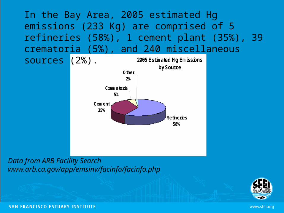
2005 Estimated Hg Emissions by Source

Refineries58%

Cement35%

Crematoria5%

Other2%

In the Bay Area, 2005 estimated Hg emissions (233 Kg) are comprised of 5 refineries (58%), 1 cement plant (35%), 39 crematoria (5%), and 240 miscellaneous sources (2%).

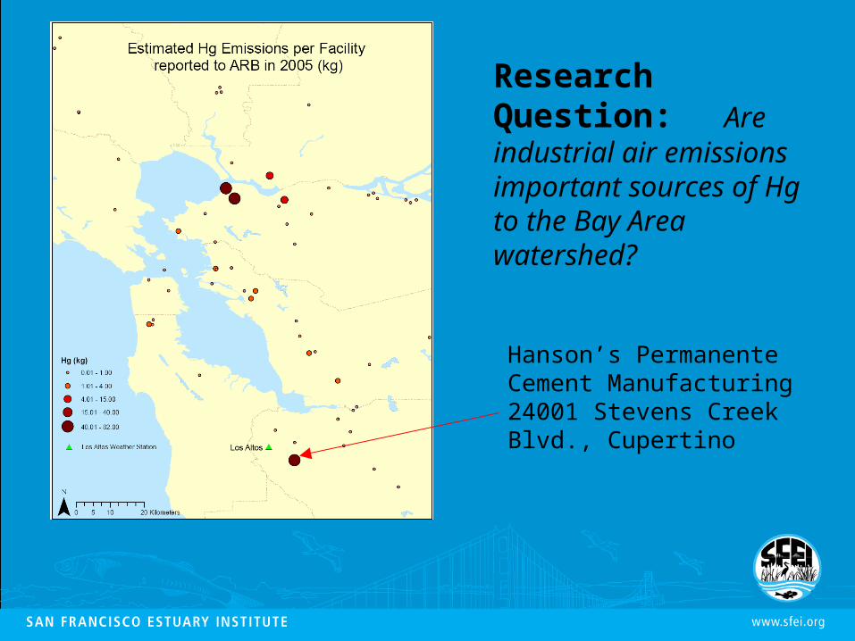
Hanson’s Permanente Cement Manufacturing24001 Stevens Creek Blvd., Cupertino

Research Question: Are industrial air emissions important sources of Hg to the Bay Area watershed?

Methods1. Dry deposition rate:

Tekran® 2537A/1130/1135

Calculate flux (Laurier et al., 2003, Lyman et al., 2007)

Compare results between 3 sites

2. Wet deposition rate:

Mercury Deposition Network collectors

Calculate flux

Compare results from 3 sites

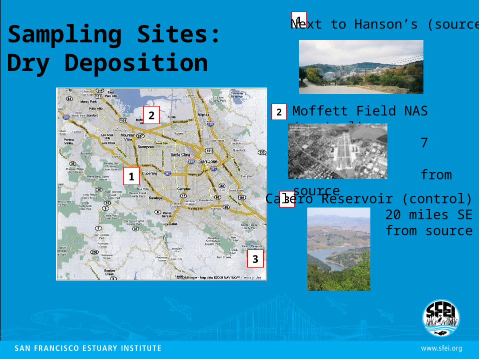
1 Next to Hanson’s (source)

1

Sampling Sites: Dry Deposition

3

2 Moffett Field NAS (control) 7 miles N from source

Calero Reservoir (control) 20 miles SE from source

3

2

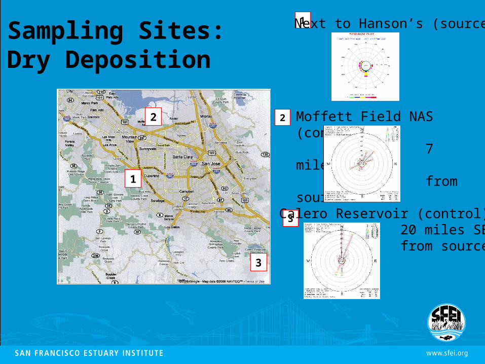
1 Next to Hanson’s (source)

1

Sampling Sites: Dry Deposition

3

2 Moffett Field NAS (control) 7 miles N from source

Calero Reservoir (control) 20 miles SE from source

3

2

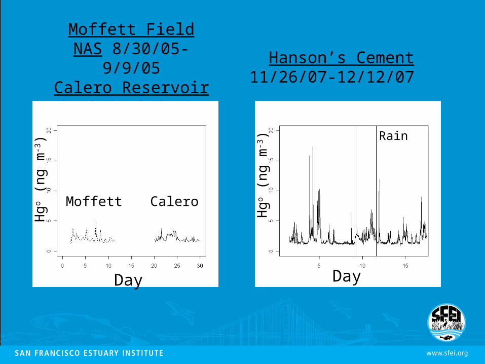
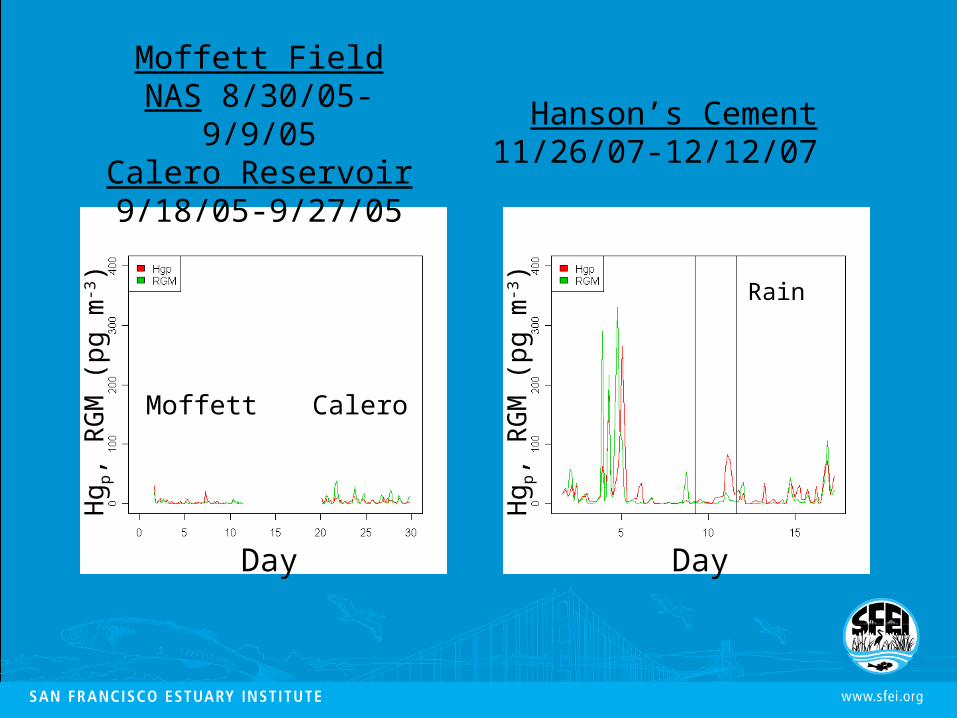
Moffett Field NAS 8/30/05-9/9/05

Calero Reservoir9/18/05-9/27/05

Hanson’s Cement11/26/07-12/12/07

DayH

go (

ng

m-3) Rain

Hg

o (

ng

m-3)

Day

Moffett Calero

Moffett Field NAS 8/30/05-9/9/05

Calero Reservoir9/18/05-9/27/05

Hanson’s Cement11/26/07-12/12/07

Hg p

, RG

M (

pg

m-3)

Moffett Calero

Day Day

Hg p

, RG

M (

pg

m-3) Rain

Hgo n(ng m-3)

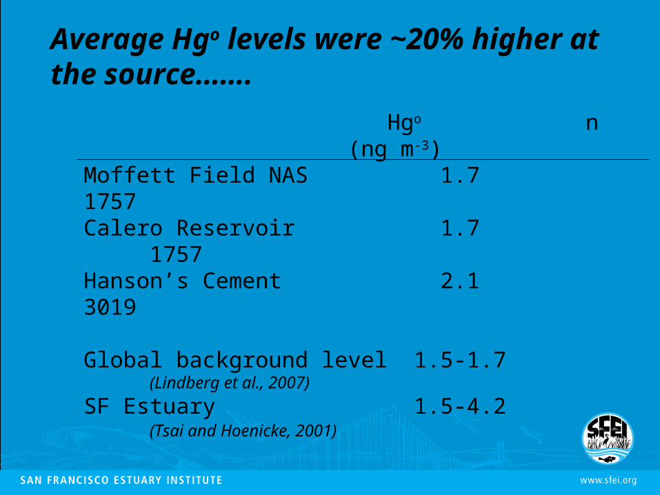
Moffett Field NAS 1.7 1757Calero Reservoir 1.7 1757Hanson’s Cement 2.1 3019

Global background level 1.5-1.7 (Lindberg et al., 2007)

SF Estuary 1.5-4.2(Tsai and Hoenicke, 2001)

Average Hgo levels were ~20% higher at the source…….

Hgp RGM n(pg m-3) (pg m-3)

Moffett Field NAS 3.1 1.8 76Calero Reservoir 4.4 6.3 76Hanson’s Cement 20 18 111

……while average Hgp and RGM levels were 6-10 times higher at the source

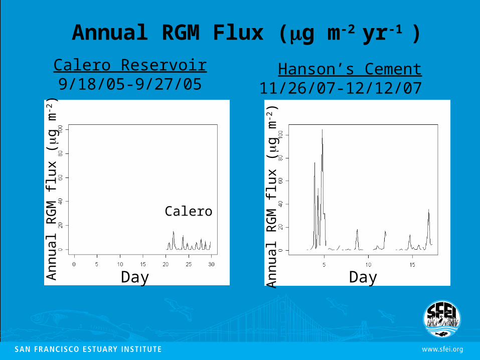
Calero Reservoir9/18/05-9/27/05

Hanson’s Cement11/26/07-12/12/07

An

nua

l RG

M fl

ux

(g

m-2)

An

nua

l RG

M fl

ux

(g

m-2)

Day Day

Calero

Annual RGM Flux (g m-2 yr-1 )

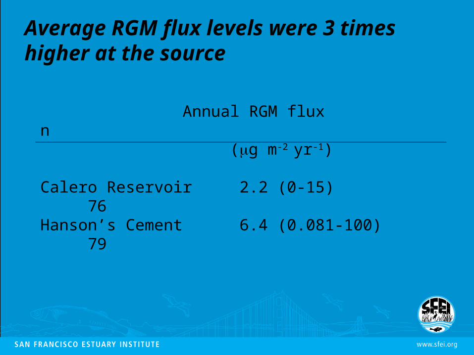
Annual RGM flux n (g m-2 yr-1)

Calero Reservoir 2.2 (0-15) 76

Hanson’s Cement 6.4 (0.081-100) 79

Average RGM flux levels were 3 times higher at the source

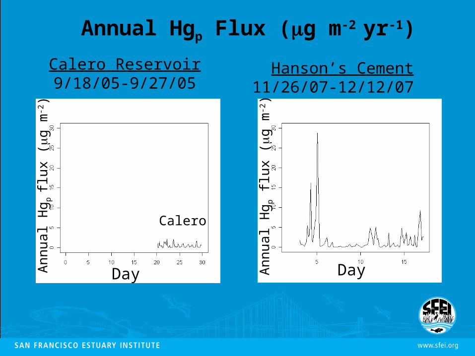
Calero Reservoir9/18/05-9/27/05

Hanson’s Cement11/26/07-12/12/07

An

nua

l Hg p

flu

x (

g m

-2)

An

nua

l Hg

p fl

ux

(g

m-2)

Day Day

Calero

Annual Hgp Flux (g m-2 yr-1)

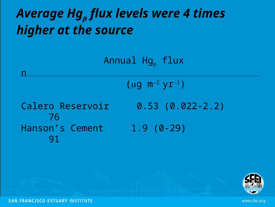
Annual Hgp flux n (g m-2 yr-1)

Calero Reservoir 0.53 (0.022-2.2) 76

Hanson’s Cement 1.9 (0-29) 91

Average Hgp flux levels were 4 times higher at the source

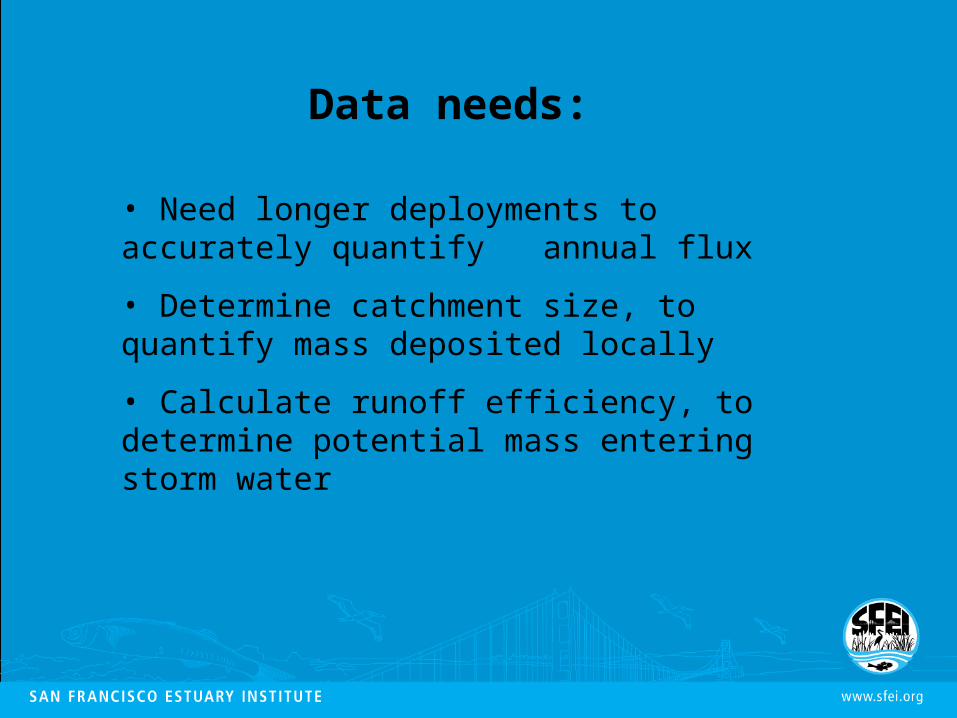
• Need longer deployments to accurately quantify annual flux

• Determine catchment size, to quantify mass deposited locally

• Calculate runoff efficiency, to determine potential mass entering storm water

Data needs:

1 Next to Hanson’s (source)

1

Sampling Sites: Wet Deposition

2

4 Moffett Field NAS (control) 7 miles N from source

De Anza College (control)2.2 miles E from source

2

4

3

3 Stevens Creek Park (control)1.5 miles S from source

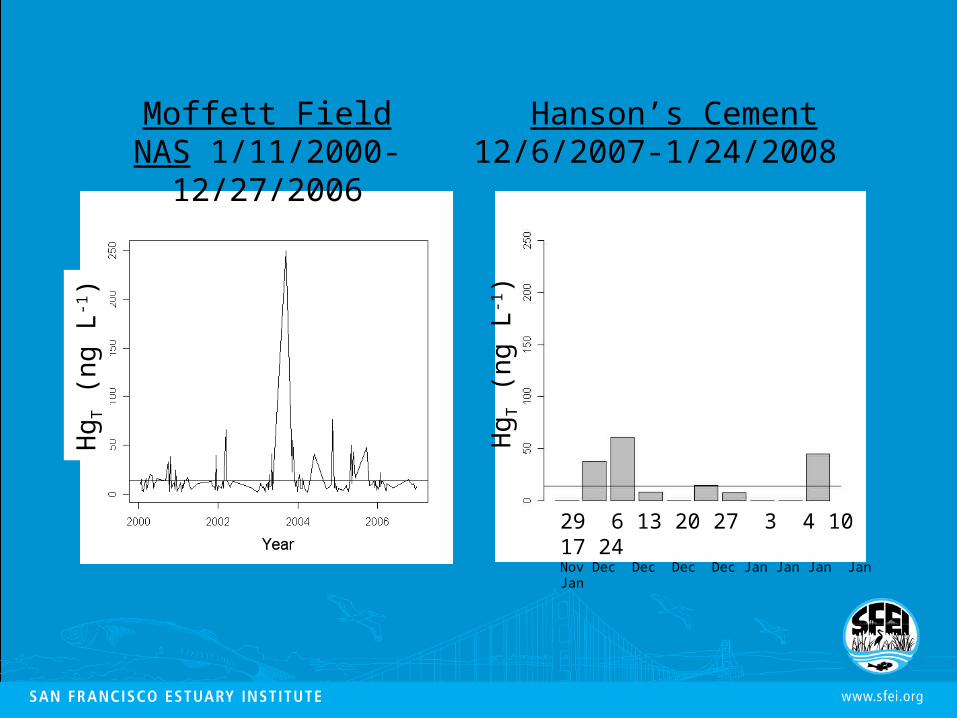
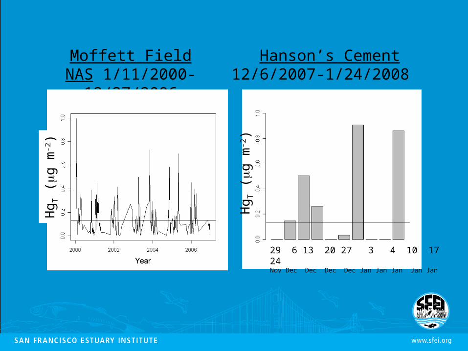
Moffett Field NAS 1/11/2000-12/27/2006

Hanson’s Cement12/6/2007-1/24/2008

Hg T

(n

g L-1

)29 6 13 20 27 3 4 10 17 24Nov Dec Dec Dec Dec Jan Jan Jan Jan Jan

Hg T

(n

g L-1

)

Moffett Field NAS 1/11/2000-12/27/2006

Hanson’s Cement12/6/2007-1/24/2008

Hg

T (g

m-2)

29 6 13 20 27 3 4 10 17 24Nov Dec Dec Dec Dec Jan Jan Jan Jan Jan

Hg

T (g

m-2)

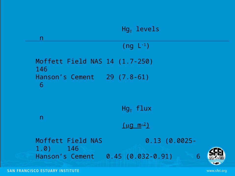
HgT levels n (ng L-1)

Moffett Field NAS 14 (1.7-250) 146

Hanson’s Cement 29 (7.8-61) 6

HgT flux n (g m-2)

Moffett Field NAS 0.13 (0.0025-1.0) 146

Hanson’s Cement 0.45 (0.032-0.91) 6

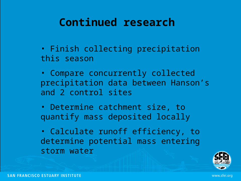
• Finish collecting precipitation this season

• Compare concurrently collected precipitation data between Hanson’s and 2 control sites

• Determine catchment size, to quantify mass deposited locally

• Calculate runoff efficiency, to determine potential mass entering storm water

Continued research

Many thanks to:

De Anza College, Environmental Studies Program, Julie Philips, Pat Cornely

Andy Lincoff, Peter Husby, and Greg Nagle from EPA, Region IX for providing Tekran support

Steve Lindberg, Mae Gustin, Eric Prestbo, and Mark Marvin-DiPasquale for their helpful advice

This study was funded through Proposition 13.

Brooks Rand, LLC for all laboratory analyses

Thank you!