AN INVESTIGATION INTO THE POWER CONSUMPTION EFFICIENCY AT A BASE METAL

REFINERY

Alzaan du Toit

In partial fulfillment of

Master of Science in Engineering (Electric Power and Energy Systems)

School of Engineering College of Agriculture, Engineering and Science

University of KwaZulu-Natal

October 2012

Examiner’s Copy Supervisor: Professor N.M. Ijumba Co-supervisor: Dr. I.G. Boake

ii

As the candidate’s Supervisor I agree/do not agree to the submission of this dissertation. Signed: ______________________________ Date: _________________

Professor N.M. Ijumba

DECLARATION

I, Alzaan du Toit declare that

(i) The research reported in this dissertation, except where otherwise indicated, is my original work.

(ii) This dissertation has not been submitted for any degree or examination at any other university.

(iii) This dissertation does not contain other persons’ data, pictures, graphs or other information, unless specifically acknowledged as being sourced from other persons.

(iv) This dissertation does not contain other persons’ writing, unless specifically

acknowledged as being sourced from other researchers. Where other written sources have been quoted, then: a) their words have been re-written but the general information attributed to them has been referenced; b) where their exact words have been used, their writing has been placed inside quotation marks, and referenced.

(v) Where I have reproduced a publication of which I am an author, co-author or editor, I have indicated in detail which part of the publication was actually written by myself alone and have fully referenced such publications.

(vi) This dissertation does not contain text, graphics or tables copied and pasted from the Internet, unless specifically acknowledged, and the source being detailed in the dissertation and in the References sections.

Signed: ________________________________ Date: __________________

iii

ACKNOWLEDGEMENTS

The author would like to express his gratitude to the following persons:

My supervisor, Professor Ijumba, for his guidance and support.

My co-supervisor, Dr. Boake, for his assistance with refinement of the study.

My wife, Cecilia, and children who perpetually supported me for the duration of this

study.

iv

ABSTRACT

The addressed topic is to investigate the power distribution at a base metal refinery and to

identify the potential improvement in power consumption efficiency. The work included in this

study revealed that the power consumption efficiency at the evaluated base metal refinery can

be improved.

The significance of this study relates to Eskom’s tariff increases and directive to mining and

large industrial companies to reduce their power consumption as well as the recent incremental

increase in power tariffs. Base metal refineries are substantial power consumers and will be

required to evaluate the efficiency of their base metal production.

A load study was conducted at a base metal refinery in order to determine the current power

consumption at the various process areas. The measurements obtained from the load study

formed the basis for calculations to determine the potential efficiency improvement. The load

study revealed that the electro-winning area contributes to the majority of the power consumed

(52% of total apparent power) at the refinery. The potential improvement in efficiency at the

electro-winning process area was identified by means of evaluating the rectifier and rectifier

transformer power consumption. Methods and technologies for the reduction in power

consumption was consequently evaluated and quantified.

The potential reduction in conductor losses by converting from global power factor correction to

localised power factor correction for the major plant areas was furthermore identified as an area

of potential efficiency improvement and consequently evaluated.

The improvement in motor efficiency across the base metal refinery was identified by means of

comparing the efficiency and power factor of high efficiency motors to that of the standard

efficiency motors installed at the refinery.

The work included in this study reveals that an improvement in power consumption efficiency

is achievable at the evaluated base metal refinery. An efficiency improvement of 1.785% (real

power reduction of 2.07%) can be achieved by implementing localised power factor correction

and high efficiency motors. An average efficiency improvement of 1.282% (total real power

reduction of 2.78%) can be achieved with the additional implementation of specialised, high

efficiency rectifier transformer designs.

v

The implementation of localised power factor correction as well as high efficiency motors was

identified as short term efficiency improvement projects. A financial study was conducted in

order to determine the cost and payback period associated with the reduction in real power

consumption for implementation of the recommended efficiency improvement projects. The

payback period, required to achieve an average efficiency improvement of 1.785%, was

calculated to be approximately 4 years. The initial capital investment required to implement the

efficiency improvement projects is about R22.5 million. The monthly electricity utility bill

savings associated with the efficiency improvement projects is approximately R455,000.

vi

NOMENCLATURE

A Conductor cross-sectional area m2

E Standard electrode potential under non-standard conditions V

oE Standard electrode potential under standard conditions V

F Faraday constant J/V.mol

tF Nett cash flow for a variable period ZAR

1aI Rectifier primary fundamental line current A

dI Rectifier DC output current A

lI Conductor current A

primaryI Transformer primary winding current A

ondaryI sec Transformer secondary winding current A

L Conductor length m

conductorL Conductor length measured as part of the load study m

sL Source inductance H

n Number of moles transferred -

P Three phase absorbed power W

copperP Transformer winding power losses W

coreP Motor core power losses W

fwP Motor friction and winding power losses W

inP Motor input power W

lossP Total motor power losses W

outP Motor output power W

outP Transformer output power W

rotorP Motor rotor power losses W

statorP Motor stator winding power losses W

strayP Motor stray power losses W

PF Thryristor rectifier power factor -

studyloadPF Power factor as measured during the load study -

Q Reaction quotient -

vii

R Gas constant J/K.mol

windingR Winding resistance Ω

primaryR Transformer primary winding resistance Ω

ondaryRsec Transformer secondary winding resistance Ω

S Apparent power VA

studyloadS Apparent power as measured during the load study VA

T Variable temperature K

0T Reference temperature K

u Thyristor commutation interval rad

LLV Rectifier primary line voltage V

llV Conductor line voltage V

dV Rectifier DC output voltage V

conductorZ Conductor impedance Ω/km

GREEK SYMBOLS

α Thyristor firing angle rad

α Temperature coefficient of resistivity K-1

η Efficiency %

dirη Motor efficiency calculated by the direct method -

indirη Motor efficiency calculated by the indirect method -

π Constant, the ratio of a circle's circumference to its diameter -

ρ Variable resistivity Ωm

0ρ Reference resistivity Ωm

ω Angular velocity rad/s

viii

LIST OF ABBREVIATIONS

BJT Bipolar junction transistor

BMR Base Metal Refinery

DC Direct current

FFT Fast fourier transform

IE International efficiency

IEC International Electrotechnical Commission

IGBT Insulated gate bipolar transistor

IGCT Integrated gate commutated thyristors

IRR Internal rate of return

MOSFET Metal-oxide-semiconductor field effect transistor

NERSA National Energy Regulator of South Africa

NRS National Rationalized Specifications

PF Power factor

PFC Power factor correction

PGM Precious group metals

PMR Precious metal refinery

PWM Pulse-width modulation

RWW Howard and Jeremy Wood

SARS South African Revenue Service

SCR Semiconductor-controlled rectifier

TCO Total cost of ownership

THD Total harmonic distortion

VAT Value added tax

WEG Werner, Eggon and Geraldo

ix

TABLE OF CONTENTS TABLE OF CONTENTS ix

LIST OF TABLES xi

LIST OF FIGURES xii

CHAPTER 1: INTRODUCTION AND BACKGROUND 1

1.1 Introduction 1 1.2 Research problem 3 1.3 Research questions 3 1.4 Research objective 3 1.5 Hypothesis 3 1.6 Importance of this study 3 1.7 Outline of dissertation 4 CHAPTER 2: LITERATURE REVIEW 5

2.1 Base metal production and average power demand 5 2.2 Power consumption efficiency case studies 5 2.3 BMR operation background 7 2.4 High current rectifiers 10 2.4.1 Thyristor phase-controlled rectifiers 10 2.4.2 IGBT chopper-rectifiers 11 2.4.3 IGCT rectifiers 13 2.5 Transformer efficiency 13 2.5.1 Transformer design 14 2.5.2 Effect of non-linear loads 14 2.6 Motor efficiency 15 2.6.1 Determining motor efficiency 15 2.6.2 High efficiency motor cost 16 2.7 Conclusion 16 CHAPTER 3: METHODOLOGY 18

3.1 Introduction 18 3.2 Load study 19 3.3 Electro-winning rectifiers and transformers 21 3.3.1 System description 21

3.3.2 Temperature rise 23 3.3.3 Rectifier power factor 25 3.3.4 Harmonics 26

3.4 Motor efficiency 28 3.5 Localised power factor correction 28 3.6 Cost 30 3.6.1 Local power factor correction 31

3.6.1.1 Quotation 31 3.6.1.2 Parameters 31

3.6.2 Motor replacement 32 3.6.2.1 Quotation 32 3.6.2.2 Parameters 32

3.6.3 Combined evaluation 32

x

CHAPTER 4: RESULTS AND EVALUATION 34

4.1 Load study 34 4.2 Electro-winning 35 4.2.1 Rectifier and rectifier transformers 36

4.2.1.1 Temperature rise 36 4.2.1.1(a) Results 36

4.2.1.1(b) Evaluation 38 4.2.1.2 Rectifier power factor 39

4.2.1.1(a) Results 39 4.2.1.1(b) Evaluation 41

4.2.1.3 Harmonics 41 4.2.1.3(a) Results 41

4.2.1.3(b) Evaluation 41 4.3 Motor efficiency 42 4.3.1 Results 42

4.3.2 Evaluation 45 4.4 Localised power factor correction 47 4.4.1 Results 47

4.4.2 Evaluation 51 4.5 Cost 51 4.5.1 Local power factor correction 51

4.5.1.1 Quotation 51 4.5.1.2 Monthly electricity utility bill breakdown 50 4.5.1.3 Payback period 50

4.5.2 Motor replacement 51 4.5.2.1 Quotation 51 4.5.2.2 Monthly electricity utility bill breakdown 51 4.5.2.3 Payback period 51

4.5.3 Combined 52 4.5.3.1 Monthly electricity utility bill breakdown 52 4.5.3.2 Payback period 52

4.6 Synopsis 53 CHAPTER 5: CONCLUSION 55

5.1 Summary of the work 55 5.2 Summary of the results 55 5.3 Proposals for future work 58

CHAPTER 6: REFERENCES 59

xi

LIST OF TABLES

Table 2-1: Energy and average power required to manufacture base metals 5

Table 2-2: Total base metal production and average power demand 5

Table 2-3: Efficiency comparison between thyristor and IGBT rectifier systems 12

Table 3-1: Transformer parameters utilised for the calculation of transformer efficiency 23

Table 3-2: Rectifier constant parameters utilised for the calculation of rectifier power

factor 26

Table 3-3: Summary of voltage harmonic limits as per NRS 48-2 27

Table 3-4: Harmonic content with harmonic filter in operation 27

Table 3-5: Electricity utility bill parameters considering local power factor correction

implemented 32

Table 3-6: Electricity utility bill parameters considering high efficiency motor

implementation 32

Table 3-7: Electricity utility bill parameters considering local power factor correction

and high efficiency motor implementation 33

Table 4-1: Load study results 34

Table 4-2: Influence of temperature variation on transformer efficiency 38

Table 4-3: Rectifier power factor at variable firing angles 40

Table 4-4: Motor efficiency comparison 42

Table 4-5: Motor power factor comparison 44

Table 4-6: Power distribution breakdown including conductor losses 48

Table 4-7: Power factor correction quotation breakdown 49

Table 4-8: Monthly utility bill with localised power factor correction implemented 50

Table 4-9: Monthly utility bill with high efficiency motors implemented 51

Table 4-10: Monthly utility bill with high efficiency motors and localised power

factor correction implemented 52

Table 4-11: Summary of results 53

xii

LIST OF FIGURES

Figure 1-1: Eskom total supply capacity and peak demand 2

Figure 2-1: Process flow diagram of a typical base metal refinery 7

Figure 2-2: Electrochemical process illustrating the electrolytic refining of copper 9

Figure 2-3: Efficiency versus rated output voltage 12

Figure 3-1: Simplified single line diagram illustrating load study measuring points 20

Figure 3-2: Single line presentations of power distribution to the main electro-winning

process 22

Figure 4-1: Power distribution breakdown 35

Figure 4-2: Resistivity versus temperature curve for copper 37

Figure 4-3: Influence of temperature variation on transformer efficiency 37

1

CHAPTER 1: INTRODUCTION AND BACKGROUND

1.1 Introduction

Metals are divided into base metals (copper, lead, zinc and nickel) and precious metals (iridium,

osmium, palladium, platinum, rhodium, and ruthenium). First stage processing of metals

generally occurs directly after being recovered from ore deposits. The metals are then further

processed into a marketable product at base metal refineries (BMR) and precious metal

refineries (PMR). The growing demand for base metals resulted in numerous capital and

expansion projects at base metal refineries in recent years. The growth in base metal refineries

contributed to significant additional power demand world wide. Electro-winning metal

production has increased by 100% world wide between 1998 and 2008 (Aqueveque, Burgos and

Wiechmann, 2008). South Africa is ranked within the top ten base metal producers in the world

contributing 2.5% to the total nickel produced (Indexmundi, 2012). Copper is the largest base

metal produced in terms of volume with 16 million tonnes produced world wide in 2010 (World

Maps, 2012).

A typical base metal refinery with nickel as main product requires an average power demand of

33MW in order to produce 37kt nickel per annum (Intex, 2007). The 2010 average base metal

power demand was 17GW globally of which included a local demand of 113MW (see Section

2.1).

The significance of this study further relates to Eskom’s tariff increases and directive to mining

and large industrial companies to reduce their power consumption as well as the recent

incremental increase in power tariffs. Base metal refineries are substantial power consumers and

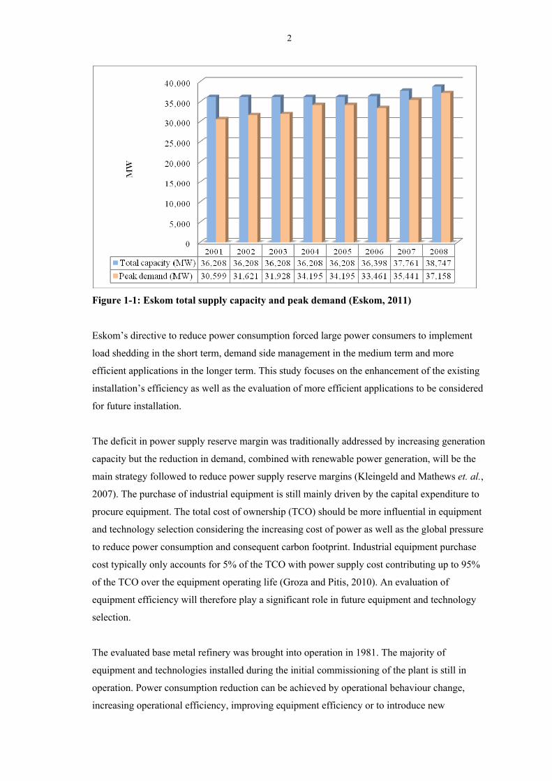
therefore contributed to the rapid depletion of South Africa’s surplus power capacity. Figure 1-1

illustrates a comparison between Eskom’s total supply capacity and peak demand between 2001

and 2008. The annual decrease in reserve margin is evident from the figure.

2

Figure 1-1: Eskom total supply capacity and peak demand (Eskom, 2011)

Eskom’s directive to reduce power consumption forced large power consumers to implement

load shedding in the short term, demand side management in the medium term and more

efficient applications in the longer term. This study focuses on the enhancement of the existing

installation’s efficiency as well as the evaluation of more efficient applications to be considered

for future installation.

The deficit in power supply reserve margin was traditionally addressed by increasing generation

capacity but the reduction in demand, combined with renewable power generation, will be the

main strategy followed to reduce power supply reserve margins (Kleingeld and Mathews et. al.,

2007). The purchase of industrial equipment is still mainly driven by the capital expenditure to

procure equipment. The total cost of ownership (TCO) should be more influential in equipment

and technology selection considering the increasing cost of power as well as the global pressure

to reduce power consumption and consequent carbon footprint. Industrial equipment purchase

cost typically only accounts for 5% of the TCO with power supply cost contributing up to 95%

of the TCO over the equipment operating life (Groza and Pitis, 2010). An evaluation of

equipment efficiency will therefore play a significant role in future equipment and technology

selection.

The evaluated base metal refinery was brought into operation in 1981. The majority of

equipment and technologies installed during the initial commissioning of the plant is still in

operation. Power consumption reduction can be achieved by operational behaviour change,

increasing operational efficiency, improving equipment efficiency or to introduce new

3

technologies (Capehart, Kennedy and Turner, 2008). The highest potential saving will be

achieved by improving equipment efficiency as well as introducing new, improved efficiency,

technologies considering the age of the existing equipment.

1.2 Research problem

Research of base metal refinery related process and electro-plating has been conducted in the

past but research in the field of power consumption efficiency at base metal refineries is very

limited. The potential for the improvement in power consumption efficiency as well as the cost

associated with the improvement has subsequently been identified as gaps.

1.3 Research questions

Can power be consumed more efficiently at a base metal refinery by means of reducing

the total absorbed real power consumption?

Is it financially viable to implement technologies, identified as part of this study, in

order to improve the power consumption efficiency at a base metal refinery?

1.4 Research objective

The objective of this study is to review the potential improvement in power consumption

efficiency at a base metal refinery from an electrical power distribution perspective and to

determine the cost associated with the potential improvement in efficiency.

1.5 Hypothesis

The reduction of real power consumption can lead to the improvement of overall plant

efficiency at a base metal refinery.

1.6 Importance of this study

This study is important because it evaluates and quantifies the potential reduction in real power

consumption at base metal refineries, in the absence of any other studies in this regard. The

perpetual increase in Eskom’s power tariffs puts increasing pressure on companies to reduce

their operating cost. The work included in this study identifies the areas and value of potential

4

operating cost savings by means of improving power consumption efficiency at base metal

refineries.

1.7 Outline of dissertation

Chapter 1 provides an introduction to the dissertation and the background to the research

problem.

Chapter 2 provides a review of the literature.

Chapter 3 provides the methodology followed to determine the power consumption efficiency

for the electro-winning area, motors and localised power factor correction. This chapter

furthermore presents the methodology followed to determine the cost associated with localised

power correction and motor replacement.

Chapter 4 present the results of the work described in Chapter 3.

Chapter 5 summarises this dissertation and provides recommendations for future research.

5

CHAPTER 2: LITERATURE REVIEW

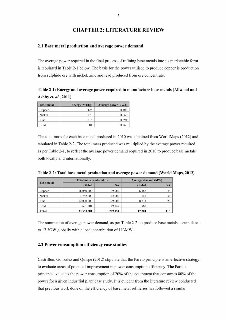
2.1 Base metal production and average power demand

The average power required in the final process of refining base metals into its marketable form

is tabulated in Table 2-1 below. The basis for the power utilised to produce copper is production

from sulphide ore with nickel, zinc and lead produced from ore concentrate.

Table 2-1: Energy and average power required to manufacture base metals (Allwood and

Ashby et. al., 2011)

Base metal Energy (MJ/kg) Average power (kW/t)

Copper 125 0.402

Nickel 270 0.868

Zinc 216 0.694

Lead 81 0.260

The total mass for each base metal produced in 2010 was obtained from WorldMaps (2012) and

tabulated in Table 2-2. The total mass produced was multiplied by the average power required,

as per Table 2-1, to reflect the average power demand required in 2010 to produce base metals

both locally and internationally.

Table 2-2: Total base metal production and average power demand (World Maps, 2012)

Base metal Total mass produced (t) Average demand (MW)

Global SA Global SA

Copper 16,080,000 109,000 6,462 44

Nickel 1,782,000 42,000 1,547 36

Zinc 12,000,000 29,002 8,333 20

Lead 3,691,301 49,149 961 13

Total 33,553,301 229,151 17,304 113

The summation of average power demand, as per Table 2-2, to produce base metals accumulates

to 17.3GW globally with a local contribution of 113MW.

2.2 Power consumption efficiency case studies

Castrillon, Gonzalez and Quispe (2012) stipulate that the Pareto principle is an effective strategy

to evaluate areas of potential improvement in power consumption efficiency. The Pareto

principle evaluates the power consumption of 20% of the equipment that consumes 80% of the

power for a given industrial plant case study. It is evident from the literature review conducted

that previous work done on the efficiency of base metal refineries has followed a similar

6

principle of focussing on a few areas that have the highest power consumption and will

consequently have the highest power savings should the efficiency of that specific area be

improved.

Aqueveque, Wiechmann and Burgos (2008) has identified the electro-winning area as the

process with the highest power demand at base metal refineries and therefore focussed on the

efficiency improvement of the transformers and rectifiers supplying power to the electro-wining

process. See Section 2.5 for an evaluation of the different rectifier technologies and a

comparison of their efficiency.

An evaluation of the process and energy efficiency in Chile at a copper mineral processing plant

was conducted by Bergh and Lo´pez et. al. (2010). The objective of the study was to perform

and evaluation of the potential abatement of carbon emissions. The authors focussed their study

on the milling area of the plant but also performed a high level evaluation of the electro-winning

area within the facility. The electro-winning area consisted of two copper cell lines operating

independently. The cell lines were fed by a 12 pulse thyristor controlled rectifier system with a

name plate rating of 13MW each. The authors evaluated a strategy of optimising transformer tap

settings, improving the rectifier operating power factor as well as the implementation of

harmonic filters. The authors achieved a combined efficiency improvement of 1.5%

implementing the proposed strategies.

A literature review of power consumption efficiency in other industries were furthermore

evaluated due to the limited research previously conducted to evaluate the power consumption

efficiency at base metal refineries from an electrical power distribution perspective. Castrillon,

Gonzalez and Quispe (2012) performed an energy efficiency evaluation and subsequent

implementation, of the efficiency improvement strategies, at a cement production plant in

Columbia. The authors identified the upgrade of the existing standard efficiency motors to high

efficiency motors as the area with highest potential efficiency improvement (0.81%) followed

by the implementation of higher efficiency lighting and air-conditioning systems (0.16%) as

well as the implementation of variable speed drives on clinker cooler motors (0.09%). The total

efficiency improvement of 1.06% resulted in a saving of 2.1 kWh per tonne cement produced.

The replacement of standard efficiency motors with high efficiency motors is the quickest

strategy for industries to improve their overall efficiency and reduce operating cost considering

that motors contribute approximately 70% to the total power consumed in the industrial sector

(Steyn, 2011). See Section 2.6 for further evaluation of motor efficiency and how it influences

this study. A study was performed by Chat-uthai, Kedsoi and Phumiphak (2005) in order to

7

compare the existing, standard efficiency motors, with high efficiency motors at an industrial

facility in Thailand. The authors used vendor nameplate efficiencies as basis for their evaluation

to achieve an average efficiency improvement of 2.58%.

2.3 BMR operation background

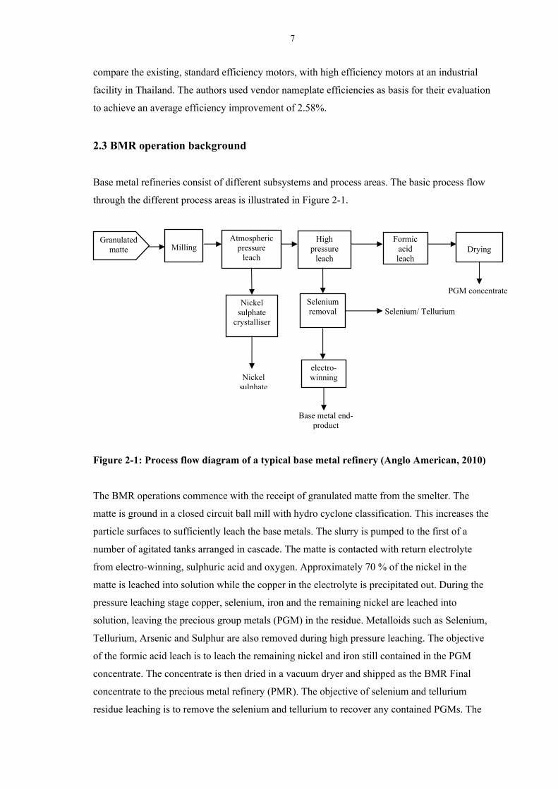
Base metal refineries consist of different subsystems and process areas. The basic process flow

through the different process areas is illustrated in Figure 2-1.

Figure 2-1: Process flow diagram of a typical base metal refinery (Anglo American, 2010)

The BMR operations commence with the receipt of granulated matte from the smelter. The

matte is ground in a closed circuit ball mill with hydro cyclone classification. This increases the

particle surfaces to sufficiently leach the base metals. The slurry is pumped to the first of a

number of agitated tanks arranged in cascade. The matte is contacted with return electrolyte

from electro-winning, sulphuric acid and oxygen. Approximately 70 % of the nickel in the

matte is leached into solution while the copper in the electrolyte is precipitated out. During the

pressure leaching stage copper, selenium, iron and the remaining nickel are leached into

solution, leaving the precious group metals (PGM) in the residue. Metalloids such as Selenium,

Tellurium, Arsenic and Sulphur are also removed during high pressure leaching. The objective

of the formic acid leach is to leach the remaining nickel and iron still contained in the PGM

concentrate. The concentrate is then dried in a vacuum dryer and shipped as the BMR Final

concentrate to the precious metal refinery (PMR). The objective of selenium and tellurium

residue leaching is to remove the selenium and tellurium to recover any contained PGMs. The

Milling

Atmospheric pressure

leach

High pressure

leach

Nickel sulphate

crystalliser

Nickel sulphate

Selenium removal Selenium/ Tellurium

electro- winning

Base metal end- product

Formic acid leach

Drying

PGM concentrate

Granulated matte

8

filtered solution from the atmospheric leach is pumped into a draft tube evaporative crystallizer

for water removal. Either nickel sulphate or sodium sulphate, depending on the type of process,

is then crystallized and dried. Sodium sulphate is sold to other industries for the production of

paper, soap, detergents and glass according to Mineral Information Institute (1998). The

electrolyte solution from the selenium and tellurium removal section is circulated through a

large number of electrolyte cells where the copper in solution is deposited onto stainless steel

(copper electro-winning) or titanium (nickel electro-winning) cathodes. The spent electrolyte is

then pumped back to the atmospheric and pressure leach circuits.

The electrochemical processes that occur during the electro-winning process form the basis for

the requirement of rectifiers and associated equipment. The copper electrochemical process is

therefore discussed below.

Electrolyte is pumped through cells containing anodes and cathodes. A positive direct current

(DC) is injected into the anode and a negative DC current is injected into the cathode. The

potential difference across the anode and cathode is determined by the reduction potential of the

electrochemical reaction. The electrolyte is typically a solution containing copper sulphate and

sulphuric acid as described by Kotz and Treichel (1999).

The basic reactions associated with copper electro-winning is described by Kotz and Treichel

(1999) as

Cu2+ (aq) + 2e- ⎯→⎯ Cu (s), (2.1)

where copper ions are reduced to solid copper on the cathode starter plates. The electrolysis of

water and oxygen at the anode is illustrated as

2H2O ⎯→⎯ 4H+ + 2O2 + 4e-. (2.2)

The net reaction may then be represented as follows:

CuSO4 + H2O ⎯→⎯ Cu + ½O + H2SO4. (2.3)

A graphical presentation of the copper electrolysis process is shown in Figure 2-2.

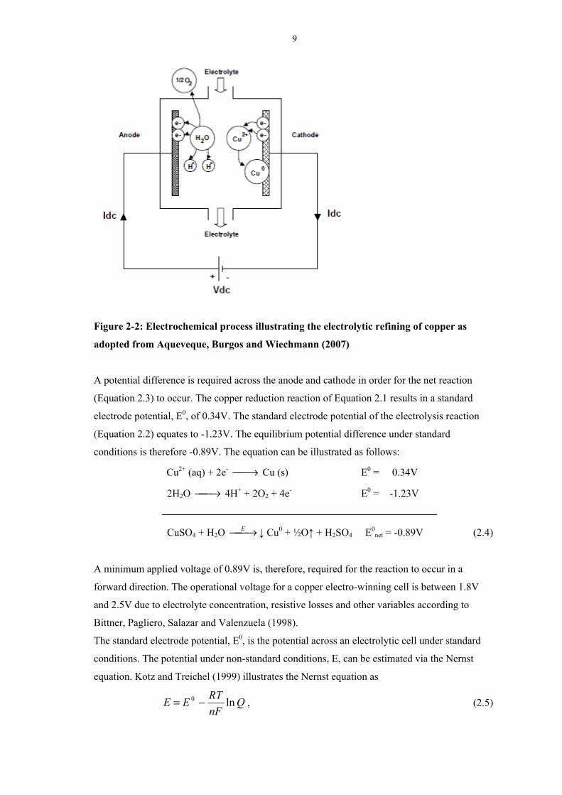
9

Figure 2-2: Electrochemical process illustrating the electrolytic refining of copper as

adopted from Aqueveque, Burgos and Wiechmann (2007)

A potential difference is required across the anode and cathode in order for the net reaction

(Equation 2.3) to occur. The copper reduction reaction of Equation 2.1 results in a standard

electrode potential, E0, of 0.34V. The standard electrode potential of the electrolysis reaction

(Equation 2.2) equates to -1.23V. The equilibrium potential difference under standard

conditions is therefore -0.89V. The equation can be illustrated as follows:

Cu2+ (aq) + 2e- ⎯→⎯ Cu (s) E0 = 0.34V

2H2O ⎯→⎯ 4H+ + 2O2 + 4e- E0 = -1.23V

CuSO4 + H2O ⎯→⎯E ↓ Cu0 + ½O↑ + H2SO4 E0net = -0.89V (2.4)

A minimum applied voltage of 0.89V is, therefore, required for the reaction to occur in a

forward direction. The operational voltage for a copper electro-winning cell is between 1.8V

and 2.5V due to electrolyte concentration, resistive losses and other variables according to

Bittner, Pagliero, Salazar and Valenzuela (1998).

The standard electrode potential, E0, is the potential across an electrolytic cell under standard

conditions. The potential under non-standard conditions, E, can be estimated via the Nernst

equation. Kotz and Treichel (1999) illustrates the Nernst equation as

QnF

RTEE ln0 −= , (2.5)

10

where R is the gas constant (8.314510 J/K.mol), F the Faraday constant (9.6485309 x 104

J/V.mol), n the number of moles of electrons transferred and Q the reaction quotient. The

practical Nerst equation used in chemical applications can be illustrated as

CatQn

VEE 00 25ln

0257.0−= , (2.6)

when the temperature is 298 K.

The potential difference across each cell is summated for the number of cells in series.

The total potential difference determines the rectifier output voltage rating. The voltage

at which an electro-winning rectifier operates determines the system efficiency as

further discussed in Section 2.5 below.

2.4 High current rectifiers

High current rectifiers fulfil a significant role in this study as

Semi-conductor components associated with high current rectifiers require special

characteristics to entertain high voltage blocking as well as high current carrying capacity.

Currently, there are mainly two technologies used for high current rectification, Thyristor-

controlled rectifiers and insulated gate bipolar transistor (IGBT) controlled rectifiers, as

described by Rodriguez, Pontt et.al. (2005). A third technology, integrated gate commutated

thyristors (IGCT), has recently been introduced as an alternative to the latter and the former.

The implementation of the above mentioned technologies in industrial high-current rectifiers is

discussed below.

2.4.1 Thyristor phase-controlled rectifiers

Thyristors, also known as semiconductor-controlled rectifiers (SCRs), were developed in 1957

and are still the solid state-power device with the highest power capability (Mohan, Undeland

and Robbins, 2003).

The thyristor is still the solid state-power device of choice due to its high efficiency, high

reliability, relatively low cost compared to other technologies and good load current control

(Rodriguez, Pontt et.al., 2005). Industries implementing large current rectifiers require stability

and minimal down time. The thyristor rectifier is a mature and proven technology and,

therefore, still remains the device of choice.

11

Thyristor rectifiers generate a substantial amount of current harmonics during pulse-width

modulation (PWM). Harmonic filters can be installed for harmonic compensation.

The latter does, however, add additional capital cost and components to the installation.

Thyristor rectifiers have significantly poor power factors which directly results in the generation

of a large reactive power component. Power factor correction (PFC) filters can be installed to

compensate for the poor power factor of thyristor rectifiers. Thyristor rectifiers produce higher

ripple currents than IGBTs. The electro-winning process is not especially sensitive to ripple

currents and does therefore not require further DC smoothing (Anglo American, 2010).

2.4.2 IGBT chopper-rectifiers

The IGBT was developed by combining the best qualities of the BJT (bipolar junction

transistor) and MOSFET (Metal-oxide-semiconductor field effect transistor) technologies

(Mohan, Undeland and Robbins, 2003). The BJT has lower conduction losses but longer

switching times. MOSFETs have higher conduction losses with shorter switching times. The

result of combining BJTs and MOSFETs on the same silicon wafer resulted in a device with fast

switching times and low conduction losses.

The chopper-rectifier contains a three phase diode rectifier that feeds a chopper circuit whose

output is then connected to a load. The chopper-rectifier provides a fast and dynamic current

response to load changes. The fast response of the chopper-rectifier allows for the fast detection

and bypassing of short-circuit currents. The chopper-rectifier maintains a high power factor

even if connected to dynamic loads (Rodriguez, Pontt et.al., 2005). IGBTs have higher

converter losses compared to thyristors. The chopper-rectifier system, however, proves to be

more efficient than thyristor phase-controlled systems for applications operating at a higher

voltage range (Scaini and Veerkamp, 2001). Figure 2-3 illustrates the relationship between

efficiency and DC output voltage for typical IGBT chopper rectifier systems as well as thyristor

rectifier systems for comparison. The figure furthermore illustrates that the two evaluated

rectifier systems’ efficiency difference reduces as the DC output voltage increase.

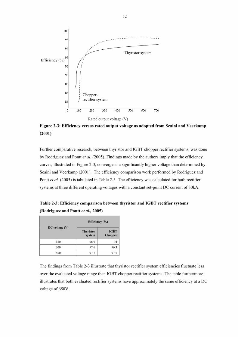
12

Figure 2-3: Efficiency versus rated output voltage as adopted from Scaini and Veerkamp

(2001)

Further comparative research, between thyristor and IGBT chopper rectifier systems, was done

by Rodriguez and Pontt et.al. (2005). Findings made by the authors imply that the efficiency

curves, illustrated in Figure 2-3, converge at a significantly higher voltage than determined by

Scaini and Veerkamp (2001). The efficiency comparison work performed by Rodriguez and

Pontt et.al. (2005) is tabulated in Table 2-3. The efficiency was calculated for both rectifier

systems at three different operating voltages with a constant set-point DC current of 30kA.

Table 2-3: Efficiency comparison between thyristor and IGBT rectifier systems

(Rodriguez and Pontt et.al., 2005)

DC voltage (V)

Efficiency (%)

Thyristor system

IGBT Chopper

150 96.9 94

300 97.6 96.3

650 97.7 97.5

The findings from Table 2-3 illustrate that thyristor rectifier system efficiencies fluctuate less

over the evaluated voltage range than IGBT chopper rectifier systems. The table furthermore

illustrates that both evaluated rectifier systems have approximately the same efficiency at a DC

voltage of 650V.

Rated output voltage (V)

Efficiency (%)

Thyristor system

Chopper-rectifier system

13

It can be concluded, from, that there is a negligible difference between thyristor and IGBT

chopper rectifier system efficiencies at DC output voltages beyond 650V.

2.4.3 IGCT rectifiers

The implementation of IGCTs in industrial rectifiers is one of the latest technologies to be

considered as alternative to IGBTs and thyristors. The IGCT rectifier will most likely consist of

a parallel unregulated diode set followed by a three-level DC/DC converter in order to make

maximum use of the IGCT switching capacity (Yongsug and Steimer, 2009). The rectifier

topology described above shows promising signs of a high power, compact design,

comparatively lower cost and more efficient future electro-winning rectifier alternative.

Lan and Li et.al. (2010) performed a simulation of the proposed IGCT rectifier producing a DC

output of 2.5kA at 5kV. The results of the simulation reflect an efficiency of 98.46%. The

output current is significantly lower in the simulation than a typical electro-winning application

with the simulation voltage at the same order of magnitude higher.

Current research indicates that IGCT rectifier efficiency will be comparable to that of thyristor

rectifiers. IGCT rectifiers do, however, have an advantage over thyristor rectifiers since they

will operate at a constant power factor with constant harmonic distortion across a wide

operating range (Yongsug and Steimer, 2009). The reliability and maintainability of IGCT

rectifiers will have to be proven for high power industrial applications for a number of years to

come before it will be recognised as viable power converter technology.

2.5 Transformer efficiency

The transformers feeding rectifiers forms an integral part of the efficiency evaluation of the

electro-winning process. The operating characteristics of rectifiers directly influence the

efficiency of the up-stream transformers feeding the rectifiers. An evaluation of transformer

efficiency is therefore included in this study.

Damnjanovic and Feruson (2004) describe transformer losses as load losses and excitation

losses. Load losses include winding losses and stray losses. Excitation losses, also known as no-

load losses, include eddy current and hysteresis losses.

Winding losses are generally substantially higher than core losses in rectifier transformers as a

result of the flux density being restricted by its saturation value (Breslin, Hurley and Wolfle,

14

1998). Excitation losses are constant for a given applied voltage. Load losses do, however,

fluctuate with the change in load current (Baranowski and Benna et.al., 1996).

2.5.1 Transformer design

Transformers can be designed to operate more efficiently. Transformer manufacturers do not

generally design transformers with efficiency as the most important parameter due to the

additional cost associated with high efficiency transformers.

Liquid cooled transformers can be designed with lower losses than dry type transformers. The

main contributing factor is more available space for the potential increase in winding diameter

and number of turns in liquid cooled transformers (Crouse, Haggerty and Malone, 1998).

Load losses as well as excitation losses can be reduced by implementing high efficiency design

principles and material selection. Excitation losses can be reduced by up to 50% using high

grade amorphous metal as apposed to general transformer core steel (Crouse, Haggerty and

Malone, 1998). Load losses can be improved by reducing conductor current density, optimal

distribution of windings to reduce eddy currents and optimising shield design to minimise stray

losses. The conductor shape can furthermore be optimally designed to reduce the skin effect

(Crouse, Haggerty and Malone, 1998).

The typical transformer life expectancy generally equals that of the original life of plant built.

This extensive life expectancy warrants an evaluation of the specific application’s life-cycle cost

although transformer efficiencies are generally high. Crouse, Haggerty and Malone (1996)

performed life-cycle cost evaluations for lower and higher efficiency transformers. The result of

the latter study motivates the higher capital expenditure of higher efficiency transformers

considering the favourable internal rate of return (IRR) over the transformer operating life.

2.5.2 Effect of non-linear loads

The effect of non-linear loads, such as thyristor rectifiers, has an impact on transformer

efficiency. Voltage harmonics influence excitation losses and current harmonics influence load

losses. Voltage harmonics have negligible impact on the transformer excitation losses

considering that excitation losses are generally less than 10% of the winding losses

(Damnjanovic and Feruson, 2004). Non-linear loads influence stray losses caused by eddy

currents (Damnjanovic and Feruson, 2004). Each transformer’s design parameters differ but

15

eddy currents and stray losses can account for up to 0.05% of the transformer nameplate rating

(Baranowski and Benna et.al., 1996).

The influence of current harmonics is much higher in low voltage distribution systems than for

medium voltage applications. The effect of non-linear loads on transformers, specifically

designed with harmonic content in mind, have a lower influence on the transformer overall

efficiency.

The eddy currents and stray losses associated with non-linear loads are contributing factors to

rectifier transformer temperature rise but will not have a profound impact on rectifier

transformer efficiency, due the optimisation of modern transformer design where the losses

associated with non-linear loads are minimised (Baranowski and Benna et.al., 1996).

2.6 Motor efficiency

It is estimated that more than 40% of all power generated world wide are consumed by motors

and approximately 87% of the motors are three phase induction motors (Liu, Tai and Yu, 2011).

The evaluation of induction motor efficiency therefore forms an important part of this study and

is further discussed below.

2.6.1 Determining motor efficiency

Two general methods for determining motor efficiency are used. The methods are known as the

direct and indirect methods and are defined below.

The direct method for determining induction motor efficiency is (Agamloh, 2009)

in

outdir P

P=η , (2.7)

where Pout is the motor output power and Pin the motor input power. The indirect method for

determining induction motor efficiency is (Agamloh, 2009)

in

lossinindir P

PP −=η , (2.8)

where Ploss represents the total motor losses and is determined by (Agamloh, 2009)

strayrotorstatorfwcoreloss PPPPPP ++++= , (2.9)

where Pcore is the is core losses, Pcore the motor friction and winding losses, Pfw the winding and

friction losses, Pstator the stator conductor losses and Pstray the remaining stray losses which are

16

generally empirically determined and dependant on operating conditions. The methodology

used by motor suppliers to determine motor efficiencies is generally dependant on the relevant

standards their products adhere to.

Motor manufacturers are continuously performing research and development of more efficient

motor designs. Induction motor efficiency can be improved by increasing stator winding

diameter, reducing the air gap between rotor and stator, increasing the rotor and stator core

length as well as the use of cast copper as apposed to aluminium rotors (Liu, Tai and Yu, 2011).

2.6.2 High efficiency motor cost

High efficiency motors are more expensive than standard efficiency motors. A capital

expenditure premium of R2,550 is generally payable per 1% improvement in efficiency (Groza

and Pitis, 2010). The main reason for the cost premium is the higher manufacturing cost of high

efficiency motors. High efficiency induction motors typically require 15% more aluminium,

20% more copper and 35% more iron to fabricate than standard efficiency motors according to

Boglietti and Cavagnino et.al. (2004).

The additional cost associated with the procurement of high efficiency motors is justified by the

reduction in power consumption and the consequent reduction in operating cost. High efficiency

motors furthermore have lower maintenance cost and increased operating life (Boglietti,

Cavagnino et.al., 2004). A life-cycle cost analysis must be performed for specific applications

in order to quantify the benefit of high efficiency versus standard efficiency motors. The power

cost of a typical 4kW standard efficiency motor is 27 times more than its original purchase cost

(Braun, 1993). The purchase cost of the 4kW standard efficiency motor is approximately

R2,870 which will result in a power cost of R77,490 over the operating life of the motor.

2.7 Conclusion

An average power demand of 17.3GW is required to produce base metals globally and 113MW

locally. The high power demand warrants an investigation into the potential improvement in

energy efficiency of the base metal production industry.

The literature review has revealed that limited research has previously been conducted on the

power consumption efficiency at base metal refineries. Previous work has mainly focussed on

the electro-winning process. The transformers and rectifiers supplying power to the electro-

17

winning process have been identified as the foremost areas for potential efficiency

improvement.

This literature review has furthermore revealed that three phase induction motors are generally

the primary contributors towards the industry’s total power consumption. An evaluation of the

potential efficiency improvement of the base metal refinery motors will therefore be included in

this study.

18

CHAPTER 3: METHODOLOGY

3.1 Introduction

An evaluation of the power consumption efficiency at the BMR commenced with a load study

as basis. A review of the load distribution pattern is required to identify the process areas that

have the highest power demand. Efficiency improvement of the process areas with the highest

power demand will produce the most significant reduction in real power consumption, as

identified in the literature review. The load study methodology is based on measurement of

power flow to individual process plant areas followed by an evaluation of the load distribution.

The load study revealed that the electro-winning process area contributes to 52% of the total

apparent power demand and three phase induction motors consumes 36% of the total apparent

power. The Pareto principle, as discussed in Section 2.2, was therefore applied in selecting the

latter two areas as main focus for this study.

The transformers and rectifiers supplying the electrochemical process have been identified, in

the literature review and load study, as the main focus areas in the electro-winning area for this

study.

The literature review revealed that rectifier semiconductor technology is the most significant

factor influencing rectifier efficiency. The literature review furthermore revealed that the two

proven technologies suitable for high current electro-winning applications do not differ

significantly as far as efficiency is concerned. The study therefore simulates, by means of

calculation and using the existing rectifier parameters as input, the rectifier operation to evaluate

the parameters that could influence the efficiency of the rectification process. The parameters

were subsequently compared with field measurements for verification purposes.

The influence that harmonics, generated by the existing rectifiers, has on the efficiency of power

transfer between the distribution network and the electro-winning process is furthermore

evaluated. The literature review identified that harmonic content directly influence eddy

currents and stray losses, which subsequently influence rectifier transformer operating

temperature and efficiency. An evaluation of the fluctuation in transformer efficiency associated

with temperature rise has therefore been evaluated. The methodology followed a calculated

approach using the existing transformer parameters and measured rectifier load parameters as

basis.

19

The potential improvement in motor efficiency was determined by comparing the efficiency of

the existing standard efficiency motors to that of high efficiency motors. A calculated approach

was followed using motor manufacturer efficiency ratings for high efficiency motors in

comparison with the efficiencies of the existing standard efficiency motors.

The potential improvement in power factor, identified as part of this study, motivated an

investigation into the potential efficiency improvement associated with the improvement in

power factor for the BMR distribution network. A calculated approach was followed by means

of comparing conductor losses, with and without, localised power factor correction

implemented.

The capital expenditure cost associated with the implementation of localised power factor

correction and high efficiency motors were determined by obtaining budget quotations from

vendors. A calculated approach was followed to determine the monthly savings. The monthly

cost saving was determined by developing an Eskom utility bill, with and without, the

efficiency improvements implemented.

3.2 Load study

The load study conducted at the evaluated base metal refinery was performed by measuring the

apparent power as well as power factor for the individual process areas. The apparent power

was measured in order to develop a distribution comparison between the different plant areas.

The power distribution was used to determine the areas with the highest power demand which

will ultimately form core of this study.

Measurements were taken three times at the BMR in order to ensure that process surges and

equipment, which are switched off for maintenance purposes, do not distort the load study

results. Measurements were therefore also taken over a three hour period to obtain an average

result with the effect of process surges minimised. The three measurements were taken on

different days within a two week period. The CT measurement points of the load study are

illustrated in the simplified single diagram, Figure 3-1. The measurement points were selected

in close proximity to cable CT test blocks and busbar VT test blocks in order to perform the

measurements in the individual circuit breaker control panels.

A Merlin Gerin PM800 (serial number: 63230-500-224A1) power meter was used to obtain the

results illustrated in Table 4-1. The power meter was connected to the 6600/110V busbar VTs

20

and feeder circuit breaker CTs within the base metal refinery’s main consumer substation. A

summary of the load study results is discussed in Section 4.1.

Figure 3-1: Simplified singe line diagram illustrating load study measuring points

l j

l

6 .6kV Eskom

Supply 1

Copper EW Copper EW Trans fOl'lnl! Trans fOl'lnl!

Copper Service Areas 1 2

Q Measu~poirds

X~ Process Service Areas 3

6 .6.kV Eskom

Supply2

6 .6kV Eskom

Supply3

1

21

3.3 Electro-winning rectifiers and transformers

The methodology followed for the evaluation of the efficiency for different aspects of the

electro-winning process is discussed in this section. The results of the measurements and

calculations associated the electro-wining process area are discussed in Section 4.2.

3.3.1 System description

The evaluated base metal refinery has three electro-winning cell line sets operating

simultaneously. A simplified single line presentation of the three electro-winning operation sets

is reflected in Figure 3-2. The circuit comprises of two rectifier transformers feeding a thyristor-

controlled rectifier in a twelve-pulse configuration. The transformer, rectifier and cell line

ratings are illustrated in Figure 3-2. The rectifier provides a significantly large DC output that is

suitable for the required electrolytic process. The rectifier maintains a set-point DC current that

is adjustable in accordance with the process requirements for optimal plating. The rectifier DC

voltage is dependant on the number of electro-winning cells included in the circuit. Table 3-1

represents the transformer parameters utilised for performing calculations in this section.

22

Figure 3-2: Singe line presentations of power distribution to the main electro-winning

processes

1

0 Measuringpoints

208EW cells

31V/cell

0 Measuringpoints

6.6kV 2000A

Transfonn er2

6.6kV 2000A

CopperEW Transfonn er2

0 Measuringpoints

6.6kV 2000A

Transfonn er4

23

3.3.2 Temperature rise

The transformer temperature rise has a significant impact on the resistivity of transformer

windings. The increase in winding resistivity increases the winding losses of a transformer

which consequently contributes to the reduction in transformer efficiency. The literature review

concluded that eddy currents and stray losses have an insignificant contribution towards modern

rectifier transformer efficiency and is therefore not included in the evaluation.

The efficiency variation associated with transformer temperature rise was determined by means

of empirical calculations. The existing transformer parameters were used as basis for

calculations. The transformer parameters utilised to calculate the values obtained in Table 4-2

are tabulated in Table 3-1.

Table 3-1: Transformer parameters utilised for the calculation of transformer efficiency

Parameter Value

Rated apparent power (S) 9.2MVA

Winding losses (Pcopper) @ 20°C 141kW

Core losses (Ptx-core) 9.4kW

Primary voltage 6.6kV

Secondary voltage 630V

The influence of temperature rise on the six rectifier transformers, as discussed in Section

4.2.1.1, was determined by using Equation 3.4 for incremental winding temperatures between

20°C and 300°C. The transformer losses were determined using Equations 7, 8 and 9 as well as

the transformer parameters tabulated in Table 3-1. The equations used to obtain the transformer

efficiency at the different temperature intervals are described below.

Halliday, Resnick, and Walker (2001) describes the variation in resistivity with temperature as

)( 000 TT −=− αρρρ , (3.1)

where T0 is a selected reference temperature and ρ0 is the resistivity at that temperature. The

resistivity, ρ, can then be determined at different temperatures, T. The temperature coefficient of

resistivity, α , was experimentally determined to provide a suitable coefficient for temperatures

in a chosen range.

Equation 3.1 is utilised to determine the resistivity of copper at various temperatures. The

reference temperature, T0, is selected to be 293.15K (20°C) and the resistivity of copper at room

temperature is 1.69 x 10-1Ωm. Halliday, Resnick, and Walker (2001) describes the temperature

coefficient of resistivity, α, to be 4.3 x 10-3 K-1 at room temperature.

24

Figure 4-2 illustrates that there is a linear relationship between the temperature rise and

resistivity of copper. The resistivity of copper can then be used to determine the transformer

winding resistance as (Halliday, Resnick, and Walker, 2001)

A

LRwinding ρ= , (3.2)

where Rwinding represents resistance and ρ, resistivity. The conductor length is represented by L

and conductor cross-sectional area by A. The transformer conductor length and cross-sectional

area will remain constant which means that the transformer winding resistance is directly

proportional to the copper resistivity at a given temperature. The latter relationship is used in the

table illustrated by Figure 4-2 to determine the variation in transformer resistance with

temperature.

The copper winding losses was determined by (Cathey, 2001)

ondaryondaryprimaryprimarycopper RIRIP sec2sec

2 += . (3.3)

The variation in resistance therefore has a directly proportional influence on copper winding

losses for a constant load.

Table 4-2 tabulates the increase in copper winding losses with the increase in resistivity. The

transformer efficiency percentage is then calculated by (Cathey, 2001)

lossesP

P

out

out

+=

100η , (3.4)

where the losses include both, winding and core losses. Equation 3.4 was consequently used to

determine the efficiency for the transformer operating at 70°C and at 110°C as discussed in

Section 4.2.1.1(b). The difference in efficiency between the two calculated efficiencies results in

the potential transformer efficiency improvement .Figure 4-3 illustrates the variation in

transformer efficiency with temperature rise as obtained from Table 4-2. The efficiency

calculation takes the influence of varying load losses associated with temperature rise into

consideration. Stray losses are regarded as negligible for the purpose of the calculation. The

calculation furthermore employs constant eddy current and hysteresis losses with the variation

in load losses.

25

3.3.3 Rectifier power factor

Industrial rectifiers are the principal contributors to a low power factor at base metal refineries.

Significant cost penalties accompany a low power factor. The latter motivates the capital

expenditure for the implementation of power factor correction equipment.

The rectifier power factor was calculated for the rectifier operating at firing angles between 0

and 180 degrees. The existing thyristor rectifier parameters, as per Table 3-2, were used as the

basis for the power factor calculations. The calculated power factor values were validated by

measuring the rectifier input power factor under normal operating conditions.

The results of the following power factor calculations are discussed in Section 4.2.1.2.

Mohan, Undeland and Robbins (2003) describe the power factor of a three phase thyristor

rectifier as

)(cos3

uPF += απ

, (3.5)

where α represents the thyristor firing angle, or delay angle, and u the commutation interval.

The commutation interval is introduced by the network impedance supplying power to the

rectifier.

The commutation interval, in radians, is obtained by

α

ωsin2

2

LL

ds

V

ILu = , (3.6)

where Ls represents the source inductance, Id the rectifier DC output current and VLL the line

voltage on the primary side of the rectifier (Mohan, Undeland and Robbins, 2003).

Mohan, Undeland and Robbins (2003) furthermore recommend that the minimum source

inductance for rectifier applications be calculated by

1305.0

a

LLs

I

VL ≥ω , (3.7)

where Ia1 represents the rectifier primary fundamental line current. The fundamental line current

fluctuates with the change in rectifier output voltage and current set point.

26

The rectifier power factor is then calculated by producing a constant DC current at variable

firing angles and variable output voltage. The DC output voltage of the rectifier at variable

firing angles is then calculated by

ds

LLd IL

VVπωα

π3

cos23 −= . (3.8)

The DC output voltage was calculated in order to verify the results of the calculations above

with field measurements.

Table 3-2: Rectifier constant parameters utilised for the calculation of rectifier power

factor

Parameter Value

Input voltage (VLL) 629.8V

Output DC current (Id) 18kA

The rectifier parameters in Table 3-2 were included in the variables of Equations 11 to 14 in

order to produce the power factors illustrated in Table 4-3.

The variation in power factor with variation in firing angle is illustrated in Table 4-3. The power

factor is calculated with and without taking the commutation angle into consideration in order to

illustrate the influence of source inductance on the thyristor rectifier power factor. Variable DC

output voltages are produced by varying the thyristor firing angles while maintaining a constant

DC output current.

3.3.4 Harmonics

The methodology for calculating the potential reduction in harmonic content injected into the

local distribution network is discussed below.

The THD was determined for the existing rectifier set during normal operation without a

harmonic filter connected to the local distribution network. The THD with a suitable harmonic

filter connected to the local distribution network was furthermore determined. The difference

between the latter and the former was calculated as the potential reduction in THD.

The harmonic content that rectifiers inject into a distribution network is regulated by the

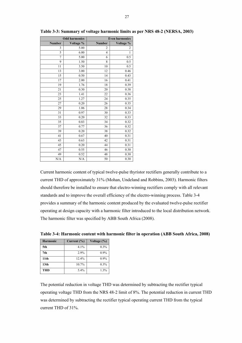
National Rationalized Specifications (NRS). Voltage harmonic content in terms of NRS 48-2 is

summarised in Table 3-3. NRS 48-2 furthermore stipulates that the total voltage harmonic

distortion must not exceed 8% for the first fourteen harmonics.

27

Table 3-3: Summary of voltage harmonic limits as per NRS 48-2 (NERSA, 2003)

Odd harmonics Even harmonics

Number Voltage % Number Voltage %

3 5.00 2 2

5 6.00 4 1

7 5.00 6 0.5

9 1.50 8 0.5

11 3.50 10 0.5

13 3.00 12 0.46

15 0.50 14 0.43

17 2.00 16 0.41

19 1.76 18 0.39

21 0.30 20 0.38

23 1.41 22 0.36

25 1.27 24 0.35

27 0.20 26 0.35

29 1.06 28 0.34

31 0.97 30 0.33

33 0.20 32 0.33

35 0.83 34 0.32

37 0.77 36 0.32

39 0.20 38 0.32

41 0.67 40 0.31

43 0.63 42 0.31

45 0.20 44 0.31

47 0.55 46 0.30

49 0.52 48 0.30

N/A N/A 50 0.30

Current harmonic content of typical twelve-pulse thyristor rectifiers generally contribute to a

current THD of approximately 31% (Mohan, Undeland and Robbins, 2003). Harmonic filters

should therefore be installed to ensure that electro-winning rectifiers comply with all relevant

standards and to improve the overall efficiency of the electro-winning process. Table 3-4

provides a summary of the harmonic content produced by the evaluated twelve-pulse rectifier

operating at design capacity with a harmonic filter introduced to the local distribution network.

The harmonic filter was specified by ABB South Africa (2008).

Table 3-4: Harmonic content with harmonic filter in operation (ABB South Africa, 2008)

Harmonic Current (%) Voltage (%)

5th 4.1% 0.3%

7th 2.9% 0.9%

11th 12.4% 0.9%

13th 10.7% 0.3%

THD 5.4% 1.3%

The potential reduction in voltage THD was determined by subtracting the rectifier typical

operating voltage THD from the NRS 48-2 limit of 8%. The potential reduction in current THD

was determined by subtracting the rectifier typical operating current THD from the typical

current THD of 31%.

28

The evaluation of the rectifier harmonic content as described above is discussed in Section

4.2.1.3.

3.4 Motor efficiency

Motors contribute to a significant portion of the base metal refinery load distribution. The

methodology followed for the analysis of the base metal refinery motor efficiency is discussed

in this section. The results and evaluation of the results are discussed in Section 4.3.

An evaluation of all the motors at the base metal refinery was conducted. All the motors and

their mechanical output power ratings were listed per plant area. The motor efficiencies and

power factors were obtained from the manufacturer data sheets for operation at 50%, 75% and

100% of full load capacity. The difference in power factor and efficiency between the existing

standard efficiency and high efficiency motors were calculated.

IEC60034-30:2008 classifies International Efficiency (IE1: standard efficiency; IE2: high

efficiency; IE3: premium efficiency) for motors.

The motors included in a leach plant as well as impurity removal motor control centre are

illustrated in Table 4-4 and Table 4-5. The motors presented in Table 4-4 and Table 4-5

accounts for approximately 8.3% of the total motors evaluated at the base metal refinery. WEG

motor manufacturer’s efficiencies were utilised to conduct the efficiency and power factor

comparison study in Table 4-4 and Table 4-5 respectively (WEG, 2009). All motors evaluated

are squirrel cage induction motors.

The total standard efficiency motor input power was calculated using the average motor

efficiency and output power as input to Equation 2.7. The calculation was repeated for high

efficiency motors. The difference in high and standard efficiency motor input power was

consequently calculated as the total potential reduction in real power consumption.

3.5 Localised power factor correction

The potential reduction in conductor losses, associated with the implementation of localised as

apposed to global power factor correction, was evaluated.

29

An evaluation of the existing conductor types, diameters and distances was conducted and a

cable schedule developed. The conductor impedance was calculated for the distribution to each

satellite substation. Conductor impedance base values were obtained from Aberdare (2010).

The conductor losses were calculated between the main consumer substation and satellite

substations of the major evaluated process areas. The conductor losses were firstly calculated

for the refinery operating at the load study power factor values, utilising the existing overall

plant power factor correction. The conductor losses were secondly determined for the scenario

where power factor correction is implemented at the satellite substations. The difference in

conductor losses, as determined above, was calculated for each conductor set and tabulated in

Section 4.4.

Conductor losses were determined by utilising the first half of Equation 3.3. The conductor

current was calculated by (Cathey, 2001)

studyloadll

lPFV

PI

3= , (3.9)

where P represents the three-phase absorbed power, Vll the line voltage and PFload study the power

factor.

The absorbed power and line voltage are constant for each calculation with the power factor the

variable. A power factor of 0.98 was utilised for the corrected power factor at satellite

substations. An average power factor of 0.98 is typically achieved when implementing local

power factor correction (ABB South Africa, 2008).

The efficiency improvement associated with the reduction in conductor losses was determined

by using Equation 2.8. The efficiency was firstly calculated with the average power factor as per

the load study and secondly with the improved power factor as 0.98. The difference in

efficiency between the two scenarios was calculated as the potential efficiency improvement.

The input power and losses obtained from Table 4-6 were used as input to Equation 2.8.

The results of the conductor losses, as described above, are illustrated and discussed in Section

4.4.

30

3.6 Cost

The methodology followed to determine the cost associated with the potential reduction in real

power consumption is discussed below. The results of the cost calculations are discussed in

Section 4.5.

A scope of work was developed and issued to vendors. Budget quotations were consequently

received from the vendors to perform the work as specified.

A quotation was obtained to install local power factor correction at satellite substations in order

to achieve the efficiency improvement as discussed in Section 4.2.1.2. A quotation was

furthermore obtained to replace the existing standard efficiency motors with high efficiency

motors in order to achieve the efficiency improvement as discussed in Section 4.3. The cost

associated with the potential reduction in rectifier transformer losses was not evaluated. The

rectifier transformer design optimisation is a specialised evaluation and not included in this

study.

The monthly Eskom electricity utility bill was calculated for the existing operation. The utility

bill was furthermore structured and calculated for the following three scenarios:

Local power factor correction implemented and the associated reduction in power

consumption reflected.

All standard efficiency motors replaced with high efficiency motors and the associated

reduction in power consumption reflected.

The combined reduction in power consumption associated with the implementation of

the work listed above.

The calculated monthly utility bill was used to determine the payback period for each of the

three scenarios above. The payback period was calculated by (Blank and Tarquin, 2002)

00

≥=

n

ttF , (3.10)

where Ft represents the net cash flow for each monthly period, t. The iterative calculation of

Equation 3.10 was repeated until the initial investment was recovered through the monthly

savings. Equation 3.10 does not take maintenance cost, timing of cash flow or the time value of

money into account. It is, however, an appropriate method considering the short investment

payback period of this study. The payback calculation reflects a conservative result considering

the lower maintenance cost of high efficiency motors in particular.

31

The evaluated base metal refinery is classified as an Eskom key customer and has a Megaflex

contract. The electricity utility bill breakdown is therefore structured in line with the Eskom

Megaflex tariff break down (Eskom, 2012). All costs exclude value added tax (VAT). Both,

Eskom and the BMR, are registered for VAT with the South African Revenue Service (SARS).

Eskom therefore excludes VAT from the BMR electricity utility bill. The monthly seasonal

based active power charge was based on 50% consumption during peak season and 50% during

off-peak season. The basis for determining the electricity utility bill and associated cost,

applicable specific to the three scenarios, are further discussed below.

An average real power consumption tariff was used for determining the active power charge.

The real power consumption, as determined by the load study, was used as the average real

power consumption for the BMR over the billing period. The tabulated real power values, in

Sections 3.6.1 and 3.6.2, were then used to calculate energy consumption for the 31 day billing

period. The improved efficiency columns were calculated by subtracting the efficiency

improvement results (see Table 4-11) from the load study results.

3.6.1 Local power factor correction

3.6.1.1 Quotation

The scope of work associated with the implementation of localised power factor correction was

developed and issued to RWW Engineering for quotation. The load study results and satellite

substation descriptions formed the basis of the scope of work. The quotation included the supply

and installation of all power factor correction equipment and associated switchgear. The

quotation base date is 22/02/2012. The quotation breakdown is tabulated in Section 4.5.1.1.

3.6.1.2 Parameters

The parameters used as input to the electricity utility bill, considering the improved power

factor and associated reduction in losses, are tabulated in Table 3-5 below.

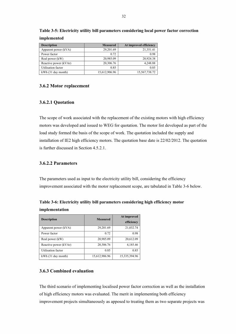
32

Table 3-5: Electricity utility bill parameters considering local power factor correction

implemented

Description Measured At improved efficiency

Apparent power (kVA) 29,201.69 21,351.41

Power factor 0.72 0.98

Real power (kW) 20,985.09 20,924.38

Reactive power (kVAr) 20,306.76 4,248.88

Utilisation factor 0.85 0.85

kWh (31 day month) 15,612,906.96 15,567,738.72

3.6.2 Motor replacement

3.6.2.1 Quotation

The scope of work associated with the replacement of the existing motors with high efficiency

motors was developed and issued to WEG for quotation. The motor list developed as part of the

load study formed the basis of the scope of work. The quotation included the supply and

installation of IE2 high efficiency motors. The quotation base date is 22/02/2012. The quotation

is further discussed in Section 4.5.2.1.

3.6.2.2 Parameters

The parameters used as input to the electricity utility bill, considering the efficiency

improvement associated with the motor replacement scope, are tabulated in Table 3-6 below.

Table 3-6: Electricity utility bill parameters considering high efficiency motor

implementation

Description Measured At improved

efficiency

Apparent power (kVA) 29,201.69 21,032.74

Power factor 0.72 0.98

Real power (kW) 20,985.09 20,612.09

Reactive power (kVAr) 20,306.76 4,185.46

Utilisation factor 0.85 0.85

kWh (31 day month) 15,612,906.96 15,335,394.96

3.6.3 Combined evaluation

The third scenario of implementing localised power factor correction as well as the installation

of high efficiency motors was evaluated. The merit in implementing both efficiency

improvement projects simultaneously as apposed to treating them as two separate projects was

33

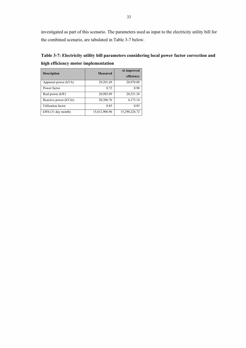
investigated as part of this scenario. The parameters used as input to the electricity utility bill for

the combined scenario, are tabulated in Table 3-7 below.

Table 3-7: Electricity utility bill parameters considering local power factor correction and

high efficiency motor implementation

Description Measured At improved

efficiency

Apparent power (kVA) 29,201.69 20,970.80

Power factor 0.72 0.98

Real power (kW) 20,985.09 20,551.38

Reactive power (kVAr) 20,306.76 4,173.14

Utilisation factor 0.85 0.85

kWh (31 day month) 15,612,906.96 15,290,226.72

34

CHAPTER 4: RESULTS AND EVALUATION

The following sections describe the results of measurements and analysis of data collected at the

electro-winning process area of the evaluated base metal refinery. The methodology of the

results obtained in this chapter is described in Chapter 3.

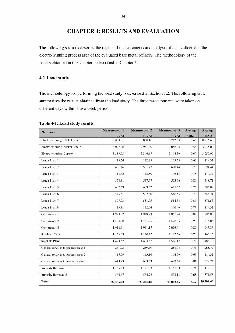
4.1 Load study

The methodology for performing the load study is described in Section 3.2. The following table

summarises the results obtained from the load study. The three measurements were taken on

different days within a two week period.

Table 4-1: Load study results

Plant area Measurement 1

(kVA)

Measurement 2

(kVA)

Measurement 3

(kVA)

Average

PF (p.u.)

Average

(kVA)

Electro-winning: Nickel Line 1 9,008.71 9,038.16 8,702.93 0.65 8,916.60

Electro-winning: Nickel Line 2 3,027.36 2,961.20 3,056.44 0.58 3,015.00

Electro-winning: Copper 3,289.03 3,346.67 3,114.30 0.69 3,250.00

Leach Plant 1 116.74 112.83 113.38 0.66 114.32

Leach Plant 2 601.16 571.72 610.44 0.75 594.44

Leach Plant 3 113.52 113.30 116.13 0.73 114.32

Leach Plant 4 554.81 537.67 553.66 0.80 548.71

Leach Plant 5 692.59 699.52 665.57 0.75 685.89

Leach Plant 6 546.81 532.80 566.53 0.72 548.71

Leach Plant 7 577.93 581.95 554.84 0.84 571.58

Leach Plant 8 113.91 112.64 116.40 0.79 114.32

Compressor 1 1,920.22 1,918.23 1,851.94 0.88 1,896.80

Compressor 2 1,534.38 1,481.25 1,528.86 0.90 1,514.83

Compressor 3 1,912.91 1,911.17 2,006.01 0.89 1,943.36

Scrubber Plant 1,156.69 1,110.22 1,162.56 0.70 1,143.15

Sulphate Plant 1,478.62 1,473.52 1,506.17 0.72 1,486.10

General services to process areas 1 281.93 289.39 286.04 0.73 285.79

General services to process areas 2 115.79 113.16 114.00 0.67 114.32

General services to process areas 3 619.93 623.63 642.64 0.94 628.73

Impurity Removal 1 1,156.73 1,121.23 1,151.50 0.74 1,143.15

Impurity Removal 2 566.67 554.92 593.13 0.65 571.58

Total 29,386.43 29,205.18 29,013.46 N/A 29,201.69

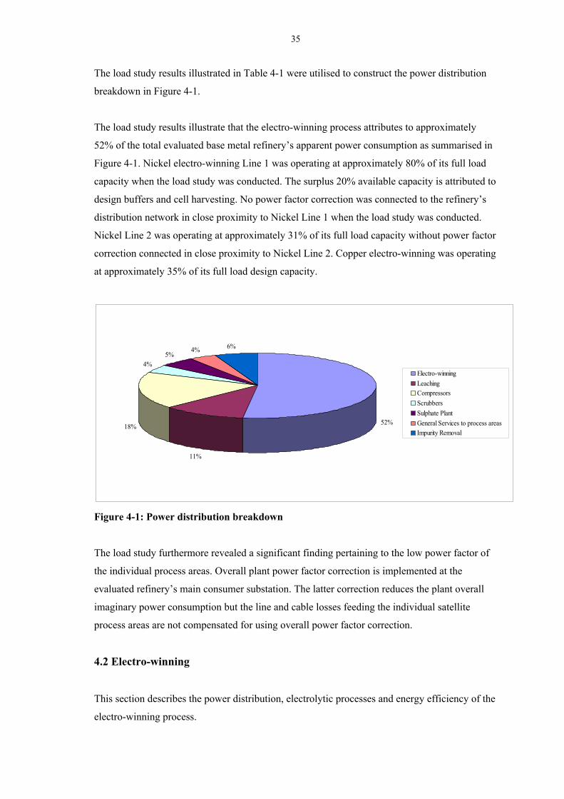
35

The load study results illustrated in Table 4-1 were utilised to construct the power distribution

breakdown in Figure 4-1.

The load study results illustrate that the electro-winning process attributes to approximately

52% of the total evaluated base metal refinery’s apparent power consumption as summarised in

Figure 4-1. Nickel electro-winning Line 1 was operating at approximately 80% of its full load

capacity when the load study was conducted. The surplus 20% available capacity is attributed to

design buffers and cell harvesting. No power factor correction was connected to the refinery’s

distribution network in close proximity to Nickel Line 1 when the load study was conducted.

Nickel Line 2 was operating at approximately 31% of its full load capacity without power factor

correction connected in close proximity to Nickel Line 2. Copper electro-winning was operating

at approximately 35% of its full load design capacity.

52%

11%

18%

4%5%

4% 6%

Electro-winning

LeachingCompressors

Scrubbers

Sulphate Plant

General Services to process areasImpurity Removal

Figure 4-1: Power distribution breakdown

The load study furthermore revealed a significant finding pertaining to the low power factor of

the individual process areas. Overall plant power factor correction is implemented at the

evaluated refinery’s main consumer substation. The latter correction reduces the plant overall

imaginary power consumption but the line and cable losses feeding the individual satellite

process areas are not compensated for using overall power factor correction.

4.2 Electro-winning

This section describes the power distribution, electrolytic processes and energy efficiency of the

electro-winning process.

36

Apparent and real power measurements were taken at a base metal refinery for each individual

process area. The measurements revealed that the electro-winning process attributes to

approximately 52% of the total apparent power of the base metal refinery on average without

taking process surges into account. The improvement in energy efficiency of the electro-

winning process will therefore result in a substantial percentile improvement for the base metal

refinery.

Copper and nickel electro-winning process operation are based on similar principles. The power

distribution to nickel and copper electro-winning circuits will remain similar except for the

rectifier DC output requirements. Different process solutions are used in the two electrolytic

processes. The materials used for anode and cathode manufacturing furthermore differ which in

turn result in different cell potentials.

4.2.1 Rectifier and rectifier transformers

This section summarises the results of the measurements and calculations performed in order to

determine the rectifier and associated transformer efficiency at different operating levels. This

section furthermore analyses the influence that certain parameters have on the efficiency of the

rectifiers and associated transformers.

4.2.1.1 Temperature rise

The influence of temperature rise on the evaluated transformers’ efficiency was determined as

per Section 3.3.2. The transformer efficiency was calculated for a range of transformer winding

temperatures. The winding resistivity and resistance were calculated at each set-point

temperature. The winding losses were subsequently calculated and then used to determine the

transformer efficiency for a given temperature. The results and evaluation of the results are

described in this section. All six transformers have the same ratings. The temperature rise

calculations were therefore performed for one transformer only and considered equal for the

other five transformers.

4.2.1.1(a) Results

Equation 3.1 was used to determine the fluctuation in resistivity with temperature rise. The

result is shown in Figure 4-2 below. The results from Equation 3.1 were used in Equation 3.2 to

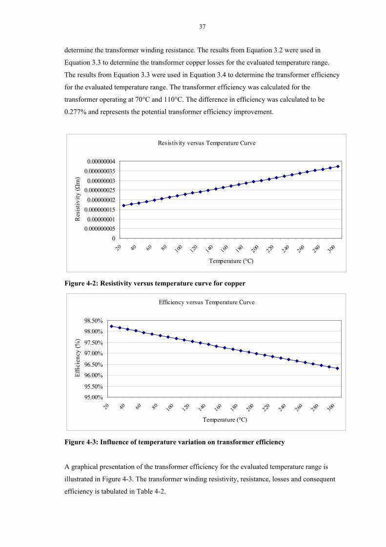
37

determine the transformer winding resistance. The results from Equation 3.2 were used in

Equation 3.3 to determine the transformer copper losses for the evaluated temperature range.

The results from Equation 3.3 were used in Equation 3.4 to determine the transformer efficiency

for the evaluated temperature range. The transformer efficiency was calculated for the

transformer operating at 70°C and 110°C. The difference in efficiency was calculated to be

0.277% and represents the potential transformer efficiency improvement.

Resistivity versus Temperature Curve

0

0.000000005

0.00000001

0.000000015

0.00000002

0.000000025

0.00000003

0.000000035

0.00000004

20 40 60 80100 120 140 160 180 200 220 240 260 280 300

Temperature (°C)

Res

isti

vity

(Ωm

)

Figure 4-2: Resistivity versus temperature curve for copper

Efficiency versus Temperature Curve

95.00%

95.50%

96.00%

96.50%

97.00%

97.50%

98.00%

98.50%

20 40 60 80100 120 140 160 180 200 220 240 260 280 300

Temperature (°C)

Eff

icie

ncy

(%)

Figure 4-3: Influence of temperature variation on transformer efficiency

A graphical presentation of the transformer efficiency for the evaluated temperature range is

illustrated in Figure 4-3. The transformer winding resistivity, resistance, losses and consequent

efficiency is tabulated in Table 4-2.

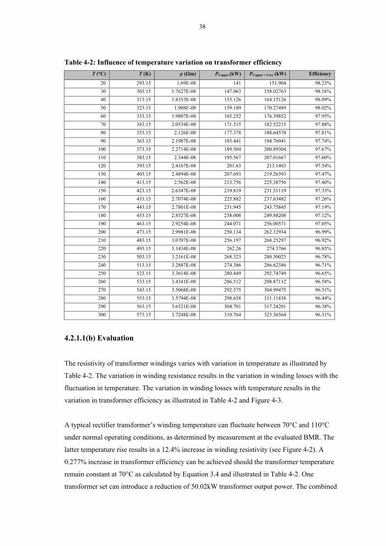
38

Table 4-2: Influence of temperature variation on transformer efficiency

T (°C) T (K) ρ (Ωm) PCopper (kW) PCopper + Core (kW) Efficiency

20 293.15 1.69E-08 141 151.904 98.23%

30 303.15 1.7627E-08 147.063 158.02763 98.16%

40 313.15 1.8353E-08 153.126 164.15126 98.09%

50 323.15 1.908E-08 159.189 170.27489 98.02%

60 333.15 1.9807E-08 165.252 176.39852 97.95%

70 343.15 2.0534E-08 171.315 182.52215 97.88%

80 353.15 2.126E-08 177.378 188.64578 97.81%

90 363.15 2.1987E-08 183.441 194.76941 97.74%

100 373.15 2.2714E-08 189.504 200.89304 97.67%

110 383.15 2.344E-08 195.567 207.01667 97.60%

120 393.15 2.4167E-08 201.63 213.1403 97.54%

130 403.15 2.4894E-08 207.693 219.26393 97.47%

140 413.15 2.562E-08 213.756 225.38756 97.40%

150 423.15 2.6347E-08 219.819 231.51119 97.33%

160 433.15 2.7074E-08 225.882 237.63482 97.26%

170 443.15 2.7801E-08 231.945 243.75845 97.19%

180 453.15 2.8527E-08 238.008 249.88208 97.12%

190 463.15 2.9254E-08 244.071 256.00571 97.05%

200 473.15 2.9981E-08 250.134 262.12934 96.99%

210 483.15 3.0707E-08 256.197 268.25297 96.92%

220 493.15 3.1434E-08 262.26 274.3766 96.85%

230 503.15 3.2161E-08 268.323 280.50023 96.78%

240 513.15 3.2887E-08 274.386 286.62386 96.71%

250 523.15 3.3614E-08 280.449 292.74749 96.65%

260 533.15 3.4341E-08 286.512 298.87112 96.58%

270 543.15 3.5068E-08 292.575 304.99475 96.51%

280 553.15 3.5794E-08 298.638 311.11838 96.44%

290 563.15 3.6521E-08 304.701 317.24201 96.38%

300 573.15 3.7248E-08 310.764 323.36564 96.31%

4.2.1.1(b) Evaluation

The resistivity of transformer windings varies with variation in temperature as illustrated by

Table 4-2. The variation in winding resistance results in the variation in winding losses with the

fluctuation in temperature. The variation in winding losses with temperature results in the

variation in transformer efficiency as illustrated in Table 4-2 and Figure 4-3.

A typical rectifier transformer’s winding temperature can fluctuate between 70°C and 110°C

under normal operating conditions, as determined by measurement at the evaluated BMR. The

latter temperature rise results in a 12.4% increase in winding resistivity (see Figure 4-2). A

0.277% increase in transformer efficiency can be achieved should the transformer temperature

remain constant at 70°C as calculated by Equation 3.4 and illustrated in Table 4-2. One

transformer set can introduce a reduction of 50.02kW transformer output power. The combined

39

potential reduction in transformer output power is therefore 150.06kW with an associated

efficiency improvement of 0.277%.

The thermodynamic design of the transformer must be optimised in combination with forced

cooling techniques in order to reduce the transformer temperature rise. The efficiency

improvement, as calculated above, does not take additional cooling power requirements into

consideration. The development of a new higher efficiency transformer will result in new

transformer parameters and consequently influence the transformer efficiency calculations

above. A detailed transformer design will have to be conducted before the actual effect of

cooling losses on the overall transformer efficiency can be evaluated.

4.2.1.2 Rectifier power factor

The methodology for calculating the rectifier input power factor at different firing angles is

discussed in Section 3.3.3. The results and evaluation of the result are discussed below.

4.2.1.2(a) Results

Equation 3.5 was used to calculate the power factor, Equation 3.6 for the commutation interval,

Equation 3.7 for the rectifier input inductance and Equation 3.8 for the rectifier DC output

voltage. The results are of the latter calculations at different firing angles are tabulated in Table

4-3.

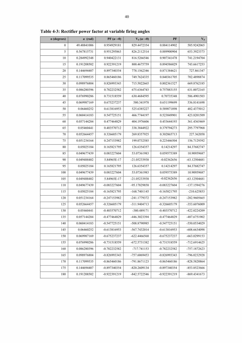
40

Table 4-3: Rectifier power factor at variable firing angles

α (degrees) u (rad) PF (u→0) Vd (u→0) PF Vd

0 49.48841006 0.954929181 829.4472354 0.884114902 585.9242065

5 0.567815731 0.951295863 826.2112514 0.889900904 653.3923373

10 0.284992348 0.940422131 816.5266546 0.907341478 741.2194704

15 0.191208502 0.922391219 800.4675759 0.894586029 743.6617253

20 0.144694407 0.897340354 778.1562346 0.871384621 727.861347

25 0.117099535 0.865460186 749.7624335 0.840361705 702.4898874

30 0.098976804 0.826993343 715.5022665 0.802361527 669.8762185

35 0.086280396 0.782232582 675.6364743 0.757883155 631.0072165

40 0.076990286 0.731518559 630.4684595 0.70735348 586.4901503

45 0.069987169 0.675237237 580.341978 0.651199699 536.8141698

50 0.06460252 0.613816953 525.6385227 0.589871898 482.4375012

55 0.060414183 0.547725151 466.7744197 0.523849901 423.8201509

60 0.057144284 0.477464829 404.1976606 0.453644193 361.4365469

65 0.05460441 0.403570712 338.3844922 0.379794273 295.7797968

70 0.052664457 0.326605179 269.8357925 0.302865713 227.362058

75 0.051234164 0.247153982 199.0732585 0.223446504 156.7129392

80 0.05025184 0.165821795 126.6354357 0.14214297 84.37682747

85 0.049677439 0.083227604 53.07361983 0.059575389 10.90959687

90 0.049488402 5.84965E-17 -21.05233938 -0.02362656 -63.12504681

95 0.05025184 0.165821795 126.6354357 0.14214297 84.37682747

100 0.049677439 0.083227604 53.07361983 0.059575389 10.90959687

105 0.049488402 5.84965E-17 -21.05233938 -0.02362656 -63.12504681

110 0.049677439 -0.083227604 -95.17829858 -0.083227604 -137.1594276

115 0.05025184 -0.165821795 -168.7401145 -0.165821795 -210.625853

120 0.051234164 -0.247153982 -241.1779372 -0.247153982 -282.9605665

125 0.052664457 -0.326605179 -311.9404713 -0.326605179 -353.6076009

130 0.05460441 -0.403570712 -380.489171 -0.403570712 -422.0224209

135 0.057144284 -0.477464829 -446.3023394 -0.477464829 -487.6751902

140 0.060414183 -0.547725151 -508.8790985 -0.547725151 -550.0534029

145 0.06460252 -0.613816953 -567.7432014 -0.613816953 -608.6634098

150 0.069987169 -0.675237237 -622.4466568 -0.675237237 -663.0299153

155 0.076990286 -0.731518559 -672.5731382 -0.731518559 -712.6914625

160 0.086280396 -0.782232582 -717.741153 -0.782232582 -757.1872623

165 0.098976804 -0.826993343 -757.6069453 -0.826993343 -796.0232928

170 0.117099535 -0.865460186 -791.8671123 -0.865460186 -828.5820864

175 0.144694407 -0.897340354 -820.2609134 -0.897340354 -853.8523666

180 0.191208502 -0.922391219 -842.5722546 -0.922391219 -869.4341673

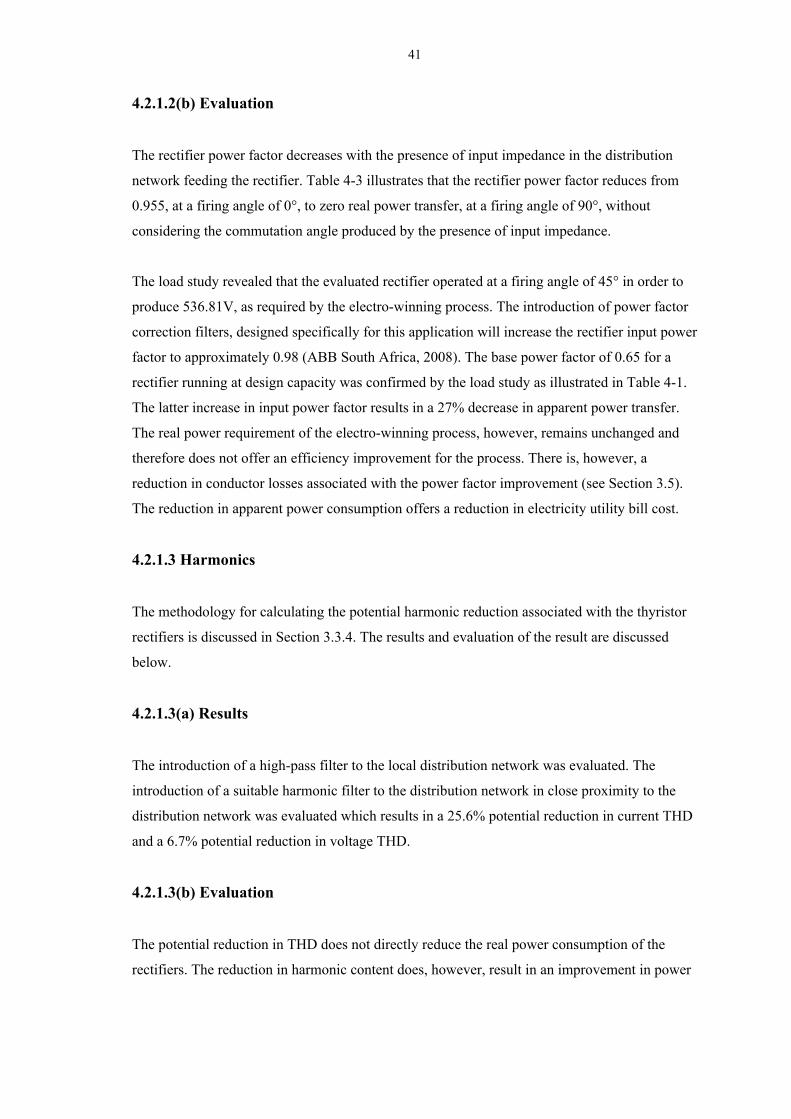
41

4.2.1.2(b) Evaluation

The rectifier power factor decreases with the presence of input impedance in the distribution

network feeding the rectifier. Table 4-3 illustrates that the rectifier power factor reduces from

0.955, at a firing angle of 0°, to zero real power transfer, at a firing angle of 90°, without

considering the commutation angle produced by the presence of input impedance.

The load study revealed that the evaluated rectifier operated at a firing angle of 45° in order to

produce 536.81V, as required by the electro-winning process. The introduction of power factor

correction filters, designed specifically for this application will increase the rectifier input power

factor to approximately 0.98 (ABB South Africa, 2008). The base power factor of 0.65 for a

rectifier running at design capacity was confirmed by the load study as illustrated in Table 4-1.

The latter increase in input power factor results in a 27% decrease in apparent power transfer.

The real power requirement of the electro-winning process, however, remains unchanged and

therefore does not offer an efficiency improvement for the process. There is, however, a

reduction in conductor losses associated with the power factor improvement (see Section 3.5).

The reduction in apparent power consumption offers a reduction in electricity utility bill cost.

4.2.1.3 Harmonics

The methodology for calculating the potential harmonic reduction associated with the thyristor

rectifiers is discussed in Section 3.3.4. The results and evaluation of the result are discussed

below.

4.2.1.3(a) Results

The introduction of a high-pass filter to the local distribution network was evaluated. The

introduction of a suitable harmonic filter to the distribution network in close proximity to the

distribution network was evaluated which results in a 25.6% potential reduction in current THD

and a 6.7% potential reduction in voltage THD.

4.2.1.3(b) Evaluation

The potential reduction in THD does not directly reduce the real power consumption of the

rectifiers. The reduction in harmonic content does, however, result in an improvement in power

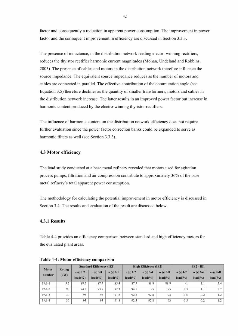
42

factor and consequently a reduction in apparent power consumption. The improvement in power

factor and the consequent improvement in efficiency are discussed in Section 3.3.3.

The presence of inductance, in the distribution network feeding electro-winning rectifiers,

reduces the thyistor rectifier harmonic current magnitudes (Mohan, Undeland and Robbins,

2003). The presence of cables and motors in the distribution network therefore influence the

source impedance. The equivalent source impedance reduces as the number of motors and

cables are connected in parallel. The effective contribution of the commutation angle (see

Equation 3.5) therefore declines as the quantity of smaller transformers, motors and cables in

the distribution network increase. The latter results in an improved power factor but increase in

harmonic content produced by the electro-winning thyristor rectifiers.

The influence of harmonic content on the distribution network efficiency does not require

further evaluation since the power factor correction banks could be expanded to serve as

harmonic filters as well (see Section 3.3.3).

4.3 Motor efficiency

The load study conducted at a base metal refinery revealed that motors used for agitation,

process pumps, filtration and air compression contribute to approximately 36% of the base

metal refinery’s total apparent power consumption.

The methodology for calculating the potential improvement in motor efficiency is discussed in

Section 3.4. The results and evaluation of the result are discussed below.

4.3.1 Results

Table 4-4 provides an efficiency comparison between standard and high efficiency motors for

the evaluated plant areas.

Table 4-4: Motor efficiency comparison

Motor

number

Rating

(kW)

Standard Efficiency (IE1) High Efficiency (IE2) IE2 - IE1

n @ 1/2

load(%)

n @ 3/4

load(%)

n @ full

load(%)

n @ 1/2

load(%)

n @ 3/4

load(%)

n @ full

load(%)

n @ 1/2

load(%)

n @ 3/4

load(%)

n @ full

load(%)

PA1-1 5.5 88.5 87.7 85.4 87.5 88.8 88.8 -1 1.1 3.4

PA1-2 90 94.2 93.9 92.3 94.5 95 95 0.3 1.1 2.7

PA1-3 30 93 93 91.8 92.5 92.8 93 -0.5 -0.2 1.2

PA1-4 30 93 93 91.8 92.5 92.8 93 -0.5 -0.2 1.2

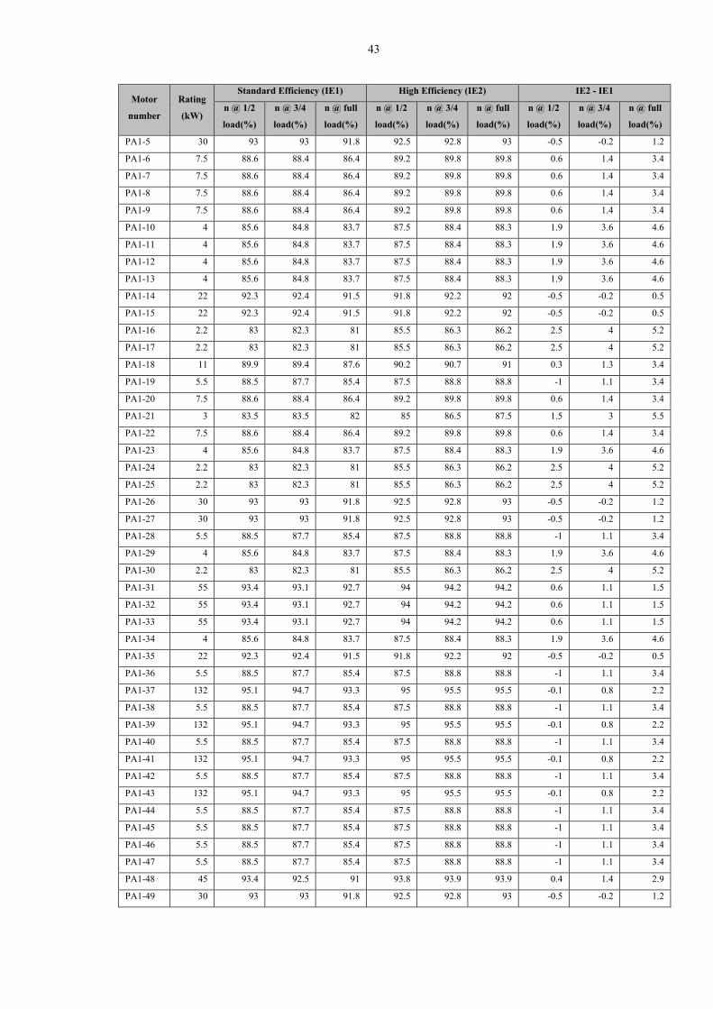
43

Motor

number

Rating

(kW)

Standard Efficiency (IE1) High Efficiency (IE2) IE2 - IE1

n @ 1/2

load(%)

n @ 3/4

load(%)

n @ full

load(%)

n @ 1/2

load(%)

n @ 3/4

load(%)

n @ full

load(%)

n @ 1/2

load(%)

n @ 3/4

load(%)

n @ full

load(%)

PA1-5 30 93 93 91.8 92.5 92.8 93 -0.5 -0.2 1.2

PA1-6 7.5 88.6 88.4 86.4 89.2 89.8 89.8 0.6 1.4 3.4

PA1-7 7.5 88.6 88.4 86.4 89.2 89.8 89.8 0.6 1.4 3.4

PA1-8 7.5 88.6 88.4 86.4 89.2 89.8 89.8 0.6 1.4 3.4

PA1-9 7.5 88.6 88.4 86.4 89.2 89.8 89.8 0.6 1.4 3.4

PA1-10 4 85.6 84.8 83.7 87.5 88.4 88.3 1.9 3.6 4.6

PA1-11 4 85.6 84.8 83.7 87.5 88.4 88.3 1.9 3.6 4.6

PA1-12 4 85.6 84.8 83.7 87.5 88.4 88.3 1.9 3.6 4.6

PA1-13 4 85.6 84.8 83.7 87.5 88.4 88.3 1.9 3.6 4.6

PA1-14 22 92.3 92.4 91.5 91.8 92.2 92 -0.5 -0.2 0.5

PA1-15 22 92.3 92.4 91.5 91.8 92.2 92 -0.5 -0.2 0.5

PA1-16 2.2 83 82.3 81 85.5 86.3 86.2 2.5 4 5.2

PA1-17 2.2 83 82.3 81 85.5 86.3 86.2 2.5 4 5.2

PA1-18 11 89.9 89.4 87.6 90.2 90.7 91 0.3 1.3 3.4

PA1-19 5.5 88.5 87.7 85.4 87.5 88.8 88.8 -1 1.1 3.4

PA1-20 7.5 88.6 88.4 86.4 89.2 89.8 89.8 0.6 1.4 3.4

PA1-21 3 83.5 83.5 82 85 86.5 87.5 1.5 3 5.5

PA1-22 7.5 88.6 88.4 86.4 89.2 89.8 89.8 0.6 1.4 3.4

PA1-23 4 85.6 84.8 83.7 87.5 88.4 88.3 1.9 3.6 4.6

PA1-24 2.2 83 82.3 81 85.5 86.3 86.2 2.5 4 5.2

PA1-25 2.2 83 82.3 81 85.5 86.3 86.2 2.5 4 5.2

PA1-26 30 93 93 91.8 92.5 92.8 93 -0.5 -0.2 1.2

PA1-27 30 93 93 91.8 92.5 92.8 93 -0.5 -0.2 1.2

PA1-28 5.5 88.5 87.7 85.4 87.5 88.8 88.8 -1 1.1 3.4

PA1-29 4 85.6 84.8 83.7 87.5 88.4 88.3 1.9 3.6 4.6

PA1-30 2.2 83 82.3 81 85.5 86.3 86.2 2.5 4 5.2

PA1-31 55 93.4 93.1 92.7 94 94.2 94.2 0.6 1.1 1.5

PA1-32 55 93.4 93.1 92.7 94 94.2 94.2 0.6 1.1 1.5

PA1-33 55 93.4 93.1 92.7 94 94.2 94.2 0.6 1.1 1.5

PA1-34 4 85.6 84.8 83.7 87.5 88.4 88.3 1.9 3.6 4.6

PA1-35 22 92.3 92.4 91.5 91.8 92.2 92 -0.5 -0.2 0.5

PA1-36 5.5 88.5 87.7 85.4 87.5 88.8 88.8 -1 1.1 3.4

PA1-37 132 95.1 94.7 93.3 95 95.5 95.5 -0.1 0.8 2.2

PA1-38 5.5 88.5 87.7 85.4 87.5 88.8 88.8 -1 1.1 3.4

PA1-39 132 95.1 94.7 93.3 95 95.5 95.5 -0.1 0.8 2.2

PA1-40 5.5 88.5 87.7 85.4 87.5 88.8 88.8 -1 1.1 3.4

PA1-41 132 95.1 94.7 93.3 95 95.5 95.5 -0.1 0.8 2.2

PA1-42 5.5 88.5 87.7 85.4 87.5 88.8 88.8 -1 1.1 3.4

PA1-43 132 95.1 94.7 93.3 95 95.5 95.5 -0.1 0.8 2.2

PA1-44 5.5 88.5 87.7 85.4 87.5 88.8 88.8 -1 1.1 3.4

PA1-45 5.5 88.5 87.7 85.4 87.5 88.8 88.8 -1 1.1 3.4

PA1-46 5.5 88.5 87.7 85.4 87.5 88.8 88.8 -1 1.1 3.4

PA1-47 5.5 88.5 87.7 85.4 87.5 88.8 88.8 -1 1.1 3.4

PA1-48 45 93.4 92.5 91 93.8 93.9 93.9 0.4 1.4 2.9

PA1-49 30 93 93 91.8 92.5 92.8 93 -0.5 -0.2 1.2

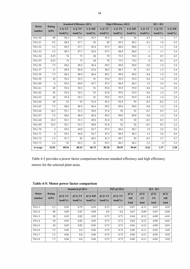
44

Motor

number

Rating

(kW)

Standard Efficiency (IE1) High Efficiency (IE2) IE2 - IE1

n @ 1/2

load(%)

n @ 3/4

load(%)

n @ full

load(%)

n @ 1/2

load(%)

n @ 3/4

load(%)

n @ full

load(%)

n @ 1/2

load(%)

n @ 3/4

load(%)

n @ full

load(%)

PA1-50 90 94.2 93.9 92.3 94.5 95 95 0.3 1.1 2.7

PA1-51 9.2 88.8 87.7 85 89 89.5 89.5 0.2 1.8 4.5

PA1-52 5.5 88.5 87.7 85.4 87.5 88.8 88.8 -1 1.1 3.4

PA1-53 5.5 88.5 87.7 85.4 87.5 88.8 88.8 -1 1.1 3.4

PA1-54 0.25 74 73 68 70 73.5 74.5 -4 0.5 6.5

PA1-55 0.25 74 73 68 70 73.5 74.5 -4 0.5 6.5

PA1-56 7.5 88.6 88.4 86.4 89.2 89.8 89.8 0.6 1.4 3.4

PA1-57 11 89.9 89.4 87.6 90.2 90.7 91 0.3 1.3 3.4

PA1-58 7.5 88.6 88.4 86.4 89.2 89.8 89.8 0.6 1.4 3.4

PA1-59 45 93.4 92.5 91 93.8 93.9 93.9 0.4 1.4 2.9

PA1-60 4 85.6 84.8 83.7 87.5 88.4 88.3 1.9 3.6 4.6

PA1-61 45 93.4 92.5 91 93.8 93.9 93.9 0.4 1.4 2.9

PA1-62 45 93.4 92.5 91 93.8 93.9 93.9 0.4 1.4 2.9

PA1-63 45 93.4 92.5 91 93.8 93.9 93.9 0.4 1.4 2.9

PA1-64 30 93 93 91.8 92.5 92.8 93 -0.5 -0.2 1.2

PA1-65 7.5 88.6 88.4 86.4 89.2 89.8 89.8 0.6 1.4 3.4

PA1-66 18.5 92.1 91.5 89.8 91.8 92 92 -0.3 0.5 2.2

PA1-67 7.5 88.6 88.4 86.4 89.2 89.8 89.8 0.6 1.4 3.4

PA1-68 18.5 92.1 91.5 89.8 91.8 92 92 -0.3 0.5 2.2

PA1-69 18.5 92.1 91.5 89.8 91.8 92 92 -0.3 0.5 2.2

PA1-70 4 85.6 84.8 83.7 87.5 88.4 88.3 1.9 3.6 4.6

PA1-71 4 85.6 84.8 83.7 87.5 88.4 88.3 1.9 3.6 4.6

PA1-72 1.5 81.7 82 80.3 81.5 84.7 85 -0.2 2.7 4.7

PA1-73 2.2 83 82.3 81 85.5 86.3 86.2 2.5 4 5.2

Average 22.81 88.94 88.42 86.75 89.20 89.99 90.04 0.26 1.57 3.28

Table 4-5 provides a power factor comparison between standard efficiency and high efficiency

motors for the selected plant areas.

Table 4-5: Motor power factor comparison

Motor

number

Rating

(kW)

Standard pf (IE1) PEP pf (IE2) IE2 - IE1

pf @ 1/2

load(%)

pf @ 3/4

load(%)

pf @ full

load(%)

pf @ 1/2

load(%)

pf @ 3/4

load(%)

pf @

full

load

pf @

1/2

load

pf @

3/4

load

pf @

full

load

PA1-1 5.5 0.85 0.79 0.85 0.72 0.72 0.87 -0.13 -0.07 0.02

PA1-2 90 0.89 0.87 0.89 0.8 0.8 0.87 -0.09 -0.07 -0.02

PA1-3 30 0.85 0.82 0.85 0.73 0.73 0.84 -0.12 -0.09 -0.01

PA1-4 30 0.85 0.82 0.85 0.73 0.73 0.84 -0.12 -0.09 -0.01

PA1-5 30 0.85 0.82 0.85 0.73 0.73 0.84 -0.12 -0.09 -0.01

PA1-6 7.5 0.86 0.8 0.86 0.75 0.75 0.88 -0.11 -0.05 0.02

PA1-7 7.5 0.86 0.8 0.86 0.75 0.75 0.88 -0.11 -0.05 0.02

PA1-8 7.5 0.86 0.8 0.86 0.75 0.75 0.88 -0.11 -0.05 0.02

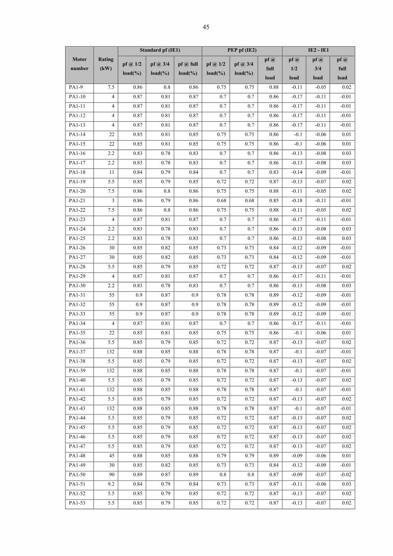
45

Motor

number

Rating

(kW)

Standard pf (IE1) PEP pf (IE2) IE2 - IE1

pf @ 1/2

load(%)

pf @ 3/4

load(%)

pf @ full

load(%)

pf @ 1/2

load(%)

pf @ 3/4

load(%)

pf @

full

load

pf @

1/2

load

pf @

3/4

load

pf @

full

load

PA1-9 7.5 0.86 0.8 0.86 0.75 0.75 0.88 -0.11 -0.05 0.02

PA1-10 4 0.87 0.81 0.87 0.7 0.7 0.86 -0.17 -0.11 -0.01

PA1-11 4 0.87 0.81 0.87 0.7 0.7 0.86 -0.17 -0.11 -0.01

PA1-12 4 0.87 0.81 0.87 0.7 0.7 0.86 -0.17 -0.11 -0.01

PA1-13 4 0.87 0.81 0.87 0.7 0.7 0.86 -0.17 -0.11 -0.01

PA1-14 22 0.85 0.81 0.85 0.75 0.75 0.86 -0.1 -0.06 0.01

PA1-15 22 0.85 0.81 0.85 0.75 0.75 0.86 -0.1 -0.06 0.01

PA1-16 2.2 0.83 0.78 0.83 0.7 0.7 0.86 -0.13 -0.08 0.03

PA1-17 2.2 0.83 0.78 0.83 0.7 0.7 0.86 -0.13 -0.08 0.03

PA1-18 11 0.84 0.79 0.84 0.7 0.7 0.83 -0.14 -0.09 -0.01

PA1-19 5.5 0.85 0.79 0.85 0.72 0.72 0.87 -0.13 -0.07 0.02

PA1-20 7.5 0.86 0.8 0.86 0.75 0.75 0.88 -0.11 -0.05 0.02

PA1-21 3 0.86 0.79 0.86 0.68 0.68 0.85 -0.18 -0.11 -0.01

PA1-22 7.5 0.86 0.8 0.86 0.75 0.75 0.88 -0.11 -0.05 0.02

PA1-23 4 0.87 0.81 0.87 0.7 0.7 0.86 -0.17 -0.11 -0.01

PA1-24 2.2 0.83 0.78 0.83 0.7 0.7 0.86 -0.13 -0.08 0.03

PA1-25 2.2 0.83 0.78 0.83 0.7 0.7 0.86 -0.13 -0.08 0.03

PA1-26 30 0.85 0.82 0.85 0.73 0.73 0.84 -0.12 -0.09 -0.01

PA1-27 30 0.85 0.82 0.85 0.73 0.73 0.84 -0.12 -0.09 -0.01

PA1-28 5.5 0.85 0.79 0.85 0.72 0.72 0.87 -0.13 -0.07 0.02

PA1-29 4 0.87 0.81 0.87 0.7 0.7 0.86 -0.17 -0.11 -0.01

PA1-30 2.2 0.83 0.78 0.83 0.7 0.7 0.86 -0.13 -0.08 0.03

PA1-31 55 0.9 0.87 0.9 0.78 0.78 0.89 -0.12 -0.09 -0.01

PA1-32 55 0.9 0.87 0.9 0.78 0.78 0.89 -0.12 -0.09 -0.01

PA1-33 55 0.9 0.87 0.9 0.78 0.78 0.89 -0.12 -0.09 -0.01

PA1-34 4 0.87 0.81 0.87 0.7 0.7 0.86 -0.17 -0.11 -0.01

PA1-35 22 0.85 0.81 0.85 0.75 0.75 0.86 -0.1 -0.06 0.01

PA1-36 5.5 0.85 0.79 0.85 0.72 0.72 0.87 -0.13 -0.07 0.02

PA1-37 132 0.88 0.85 0.88 0.78 0.78 0.87 -0.1 -0.07 -0.01

PA1-38 5.5 0.85 0.79 0.85 0.72 0.72 0.87 -0.13 -0.07 0.02

PA1-39 132 0.88 0.85 0.88 0.78 0.78 0.87 -0.1 -0.07 -0.01

PA1-40 5.5 0.85 0.79 0.85 0.72 0.72 0.87 -0.13 -0.07 0.02

PA1-41 132 0.88 0.85 0.88 0.78 0.78 0.87 -0.1 -0.07 -0.01

PA1-42 5.5 0.85 0.79 0.85 0.72 0.72 0.87 -0.13 -0.07 0.02

PA1-43 132 0.88 0.85 0.88 0.78 0.78 0.87 -0.1 -0.07 -0.01

PA1-44 5.5 0.85 0.79 0.85 0.72 0.72 0.87 -0.13 -0.07 0.02

PA1-45 5.5 0.85 0.79 0.85 0.72 0.72 0.87 -0.13 -0.07 0.02

PA1-46 5.5 0.85 0.79 0.85 0.72 0.72 0.87 -0.13 -0.07 0.02

PA1-47 5.5 0.85 0.79 0.85 0.72 0.72 0.87 -0.13 -0.07 0.02

PA1-48 45 0.88 0.85 0.88 0.79 0.79 0.89 -0.09 -0.06 0.01

PA1-49 30 0.85 0.82 0.85 0.73 0.73 0.84 -0.12 -0.09 -0.01

PA1-50 90 0.89 0.87 0.89 0.8 0.8 0.87 -0.09 -0.07 -0.02

PA1-51 9.2 0.84 0.79 0.84 0.73 0.73 0.87 -0.11 -0.06 0.03

PA1-52 5.5 0.85 0.79 0.85 0.72 0.72 0.87 -0.13 -0.07 0.02

PA1-53 5.5 0.85 0.79 0.85 0.72 0.72 0.87 -0.13 -0.07 0.02

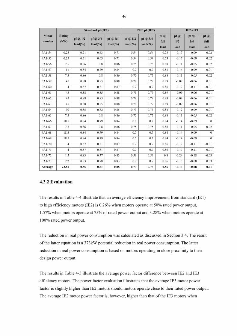
46

Motor

number

Rating

(kW)

Standard pf (IE1) PEP pf (IE2) IE2 - IE1

pf @ 1/2

load(%)

pf @ 3/4

load(%)

pf @ full

load(%)

pf @ 1/2

load(%)

pf @ 3/4

load(%)

pf @

full

load

pf @

1/2

load

pf @

3/4

load

pf @

full

load

PA1-54 0.25 0.71 0.63 0.71 0.54 0.54 0.73 -0.17 -0.09 0.02

PA1-55 0.25 0.71 0.63 0.71 0.54 0.54 0.73 -0.17 -0.09 0.02

PA1-56 7.5 0.86 0.8 0.86 0.75 0.75 0.88 -0.11 -0.05 0.02

PA1-57 11 0.84 0.79 0.84 0.7 0.7 0.83 -0.14 -0.09 -0.01

PA1-58 7.5 0.86 0.8 0.86 0.75 0.75 0.88 -0.11 -0.05 0.02

PA1-59 45 0.88 0.85 0.88 0.79 0.79 0.89 -0.09 -0.06 0.01

PA1-60 4 0.87 0.81 0.87 0.7 0.7 0.86 -0.17 -0.11 -0.01

PA1-61 45 0.88 0.85 0.88 0.79 0.79 0.89 -0.09 -0.06 0.01

PA1-62 45 0.88 0.85 0.88 0.79 0.79 0.89 -0.09 -0.06 0.01

PA1-63 45 0.88 0.85 0.88 0.79 0.79 0.89 -0.09 -0.06 0.01

PA1-64 30 0.85 0.82 0.85 0.73 0.73 0.84 -0.12 -0.09 -0.01

PA1-65 7.5 0.86 0.8 0.86 0.75 0.75 0.88 -0.11 -0.05 0.02

PA1-66 18.5 0.84 0.79 0.84 0.7 0.7 0.84 -0.14 -0.09 0

PA1-67 7.5 0.86 0.8 0.86 0.75 0.75 0.88 -0.11 -0.05 0.02

PA1-68 18.5 0.84 0.79 0.84 0.7 0.7 0.84 -0.14 -0.09 0

PA1-69 18.5 0.84 0.79 0.84 0.7 0.7 0.84 -0.14 -0.09 0

PA1-70 4 0.87 0.81 0.87 0.7 0.7 0.86 -0.17 -0.11 -0.01

PA1-71 4 0.87 0.81 0.87 0.7 0.7 0.86 -0.17 -0.11 -0.01

PA1-72 1.5 0.83 0.77 0.83 0.59 0.59 0.8 -0.24 -0.18 -0.03

PA1-73 2.2 0.83 0.78 0.83 0.7 0.7 0.86 -0.13 -0.08 0.03

Average 22.81 0.85 0.81 0.85 0.73 0.73 0.86 -0.13 -0.08 0.01

4.3.2 Evaluation

The results in Table 4-4 illustrate that an average efficiency improvement, from standard (IE1)

to high efficiency motors (IE2) is 0.26% when motors operate at 50% rated power output,

1.57% when motors operate at 75% of rated power output and 3.28% when motors operate at

100% rated power output.

The reduction in real power consumption was calculated as discussed in Section 3.4. The result

of the latter equation is a 373kW potential reduction in real power consumption. The latter

reduction in real power consumption is based on motors operating in close proximity to their

design power output.

The results in Table 4-5 illustrate the average power factor difference between IE2 and IE3

efficiency motors. The power factor evaluation illustrates that the average IE3 motor power

factor is slightly higher than IE2 motors should motors operate close to their rated power output.

The average IE2 motor power factor is, however, higher than that of the IE3 motors when

47

operating below full load design capacity. The latter finding highlights the importance of correct

motor specification when installing high efficiency motors.

4.4 Localised power factor correction

4.4.1 Results

The results of the conductor loss calculations, as discussed in Section 3.5, are illustrated below.

The following table summarises the conductor losses for the individual process areas.

The results of the conductor losses in Table 4-6 formed the basis in determining the efficiency

improvement associated with the implementation of localised power factor correction.

The total reduction in conductor losses are 60.71kW (see Table 4-6).

The conductor efficiency, associated with the load study power factor, was determined using

Equation 2.8. The losses of 133.2kW and input power of 20,985.09kW was used as input to

determine an efficiency of 0.994%.

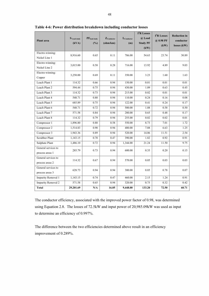
48

Table 4-6: Power distribution breakdown including conductor losses

Plant area S Load study

(kVA)

PFload study

(%)

ZConductor

(ohm/km)

LConductor

(m)

I2R Losses

@ Load

Study PF

(kW)

I2R Losses

@ 0.98 PF

(kW)

Reduction in

conductor

losses (kW)

Electro-winning:

Nickel Line 1 8,916.60 0.65 0.11 786.00 54.63 23.74 30.89

Electro-winning:

Nickel Line 2 3,015.00 0.58 0.28 716.00 13.92 4.89 9.03

Electro-winning:

Copper 3,250.00 0.69 0.11 350.00 3.23 1.60 1.63

Leach Plant 1 114.32 0.66 0.94 150.00 0.01 0.01 0.01

Leach Plant 2 594.44 0.75 0.94 430.00 1.09 0.63 0.45

Leach Plant 3 114.32 0.73 0.94 215.00 0.02 0.01 0.01

Leach Plant 4 548.71 0.80 0.94 110.00 0.24 0.16 0.08

Leach Plant 5 685.89 0.75 0.94 122.00 0.41 0.24 0.17

Leach Plant 6 548.71 0.72 0.94 500.00 1.08 0.58 0.50

Leach Plant 7 571.58 0.84 0.94 280.00 0.65 0.48 0.17

Leach Plant 8 114.32 0.79 0.94 255.00 0.02 0.02 0.01

Compressor 1 1,896.80 0.88 0.58 550.00 8.73 7.01 1.72

Compressor 2 1,514.83 0.90 0.94 480.00 7.88 6.63 1.25

Compressor 3 1,943.36 0.89 0.94 520.00 14.06 11.51 2.54

Scrubber Plant 1,143.15 0.70 0.47 390.00 1.82 0.92 0.91

Sulphate Plant 1,486.10 0.72 0.94 1,344.00 21.24 11.50 9.75

General services to

process areas 1 285.79 0.73 0.94 600.00 0.35 0.20 0.15

General services to

process areas 2 114.32 0.67 0.94 570.00 0.05 0.03 0.03

General services to

process areas 3 628.73 0.94 0.94 300.00 0.85 0.78 0.07

Impurity Removal 1 1,143.15 0.74 0.47 460.00 2.15 1.24 0.91

Impurity Removal 2 571.58 0.65 0.94 320.00 0.75 0.32 0.42

Total 29,201.69 N/A 16.05 9,448.00 133.20 72.50 60.71

The conductor efficiency, associated with the improved power factor of 0.98, was determined

using Equation 2.8. The losses of 72.5kW and input power of 20,985.09kW was used as input

to determine an efficiency of 0.997%.

The difference between the two efficiencies determined above result in an efficiency

improvement of 0.289%.

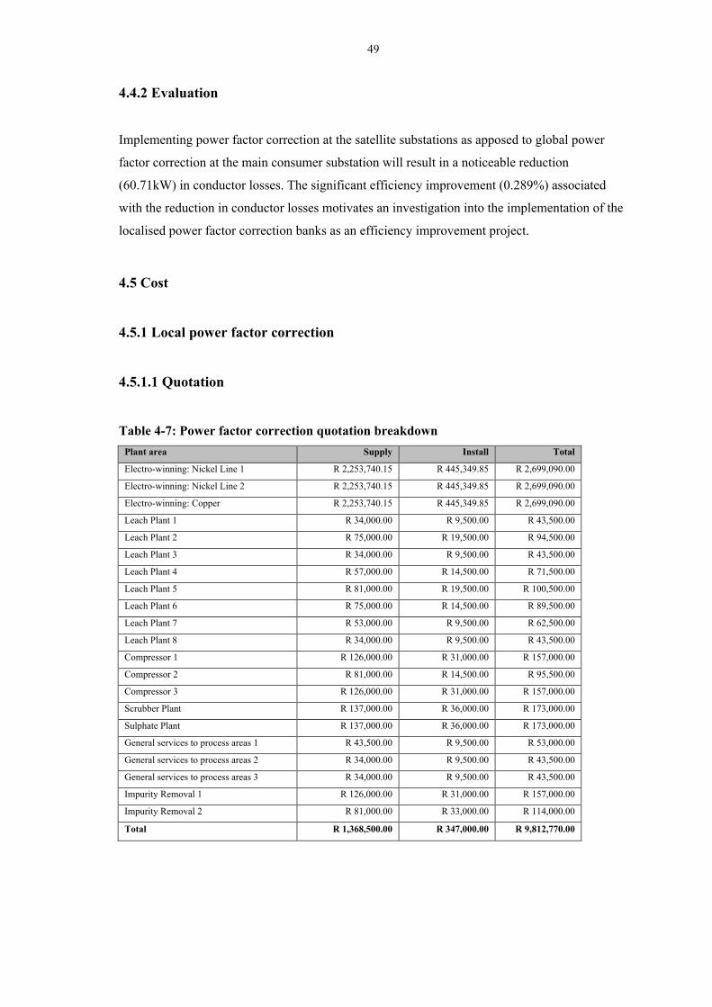
49

4.4.2 Evaluation

Implementing power factor correction at the satellite substations as apposed to global power

factor correction at the main consumer substation will result in a noticeable reduction

(60.71kW) in conductor losses. The significant efficiency improvement (0.289%) associated

with the reduction in conductor losses motivates an investigation into the implementation of the

localised power factor correction banks as an efficiency improvement project.

4.5 Cost

4.5.1 Local power factor correction

4.5.1.1 Quotation

Table 4-7: Power factor correction quotation breakdown

Plant area Supply Install Total

Electro-winning: Nickel Line 1 R 2,253,740.15 R 445,349.85 R 2,699,090.00

Electro-winning: Nickel Line 2 R 2,253,740.15 R 445,349.85 R 2,699,090.00

Electro-winning: Copper R 2,253,740.15 R 445,349.85 R 2,699,090.00

Leach Plant 1 R 34,000.00 R 9,500.00 R 43,500.00

Leach Plant 2 R 75,000.00 R 19,500.00 R 94,500.00

Leach Plant 3 R 34,000.00 R 9,500.00 R 43,500.00

Leach Plant 4 R 57,000.00 R 14,500.00 R 71,500.00

Leach Plant 5 R 81,000.00 R 19,500.00 R 100,500.00

Leach Plant 6 R 75,000.00 R 14,500.00 R 89,500.00

Leach Plant 7 R 53,000.00 R 9,500.00 R 62,500.00

Leach Plant 8 R 34,000.00 R 9,500.00 R 43,500.00

Compressor 1 R 126,000.00 R 31,000.00 R 157,000.00

Compressor 2 R 81,000.00 R 14,500.00 R 95,500.00

Compressor 3 R 126,000.00 R 31,000.00 R 157,000.00

Scrubber Plant R 137,000.00 R 36,000.00 R 173,000.00

Sulphate Plant R 137,000.00 R 36,000.00 R 173,000.00

General services to process areas 1 R 43,500.00 R 9,500.00 R 53,000.00

General services to process areas 2 R 34,000.00 R 9,500.00 R 43,500.00

General services to process areas 3 R 34,000.00 R 9,500.00 R 43,500.00

Impurity Removal 1 R 126,000.00 R 31,000.00 R 157,000.00

Impurity Removal 2 R 81,000.00 R 33,000.00 R 114,000.00

Total R 1,368,500.00 R 347,000.00 R 9,812,770.00

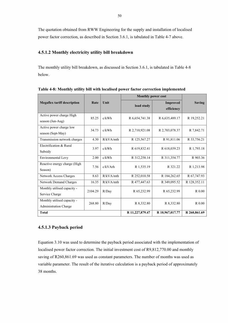
50

The quotation obtained from RWW Engineering for the supply and installation of localised

power factor correction, as described in Section 3.6.1, is tabulated in Table 4-7 above.

4.5.1.2 Monthly electricity utility bill breakdown

The monthly utility bill breakdown, as discussed in Section 3.6.1, is tabulated in Table 4-8

below.

Table 4-8: Monthly utility bill with localised power factor correction implemented

Megaflex tariff description Rate Unit

Monthly power cost

Saving load study

Improved

efficiency

Active power charge High

season (Jun-Aug) 85.25 c/kWh R 6,654,741.38 R 6,635,489.17 R 19,252.21

Active power charge low

season (Sept-May) 34.73 c/kWh R 2,710,921.08 R 2,703,078.37 R 7,842.71

Transmission network charges 4.30 R/kVA/mth R 125,567.27 R 91,811.06 R 33,756.21

Electrification & Rural

Subsidy 3.97 c/kWh R 619,832.41 R 618,039.23 R 1,793.18

Environmental Levy 2.00 c/kWh R 312,258.14 R 311,354.77 R 903.36

Reactive energy charge (High

Season) 7.56 c/kVArh R 1,535.19 R 321.22 R 1,213.98

Network Access Charges 8.63 R/kVA/mth R 252,010.58 R 184,262.65 R 67,747.93

Network Demand Charges 16.35 R/kVA/mth R 477,447.63 R 349,095.52 R 128,352.11

Monthly utilised capacity -

Service Charge 2104.29 R/Day R 65,232.99 R 65,232.99 R 0.00

Monthly utilised capacity -

Administration Charge 268.80 R/Day R 8,332.80 R 8,332.80 R 0.00

Total R 11,227,879.47 R 10,967,017.77 R 260,861.69

4.5.1.3 Payback period

Equation 3.10 was used to determine the payback period associated with the implementation of

localised power factor correction. The initial investment cost of R9,812,770.00 and monthly

saving of R260,861.69 was used as constant parameters. The number of months was used as

variable parameter. The result of the iterative calculation is a payback period of approximately

38 months.

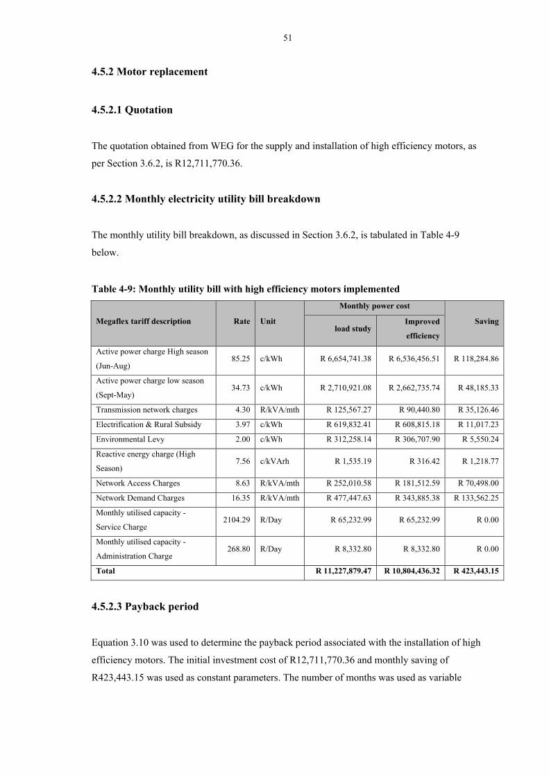
51

4.5.2 Motor replacement

4.5.2.1 Quotation

The quotation obtained from WEG for the supply and installation of high efficiency motors, as

per Section 3.6.2, is R12,711,770.36.

4.5.2.2 Monthly electricity utility bill breakdown

The monthly utility bill breakdown, as discussed in Section 3.6.2, is tabulated in Table 4-9

below.

Table 4-9: Monthly utility bill with high efficiency motors implemented

Megaflex tariff description Rate Unit

Monthly power cost

Saving load study

Improved

efficiency

Active power charge High season

(Jun-Aug) 85.25 c/kWh R 6,654,741.38 R 6,536,456.51 R 118,284.86

Active power charge low season

(Sept-May) 34.73 c/kWh R 2,710,921.08 R 2,662,735.74 R 48,185.33

Transmission network charges 4.30 R/kVA/mth R 125,567.27 R 90,440.80 R 35,126.46

Electrification & Rural Subsidy 3.97 c/kWh R 619,832.41 R 608,815.18 R 11,017.23

Environmental Levy 2.00 c/kWh R 312,258.14 R 306,707.90 R 5,550.24

Reactive energy charge (High

Season) 7.56 c/kVArh R 1,535.19 R 316.42 R 1,218.77

Network Access Charges 8.63 R/kVA/mth R 252,010.58 R 181,512.59 R 70,498.00

Network Demand Charges 16.35 R/kVA/mth R 477,447.63 R 343,885.38 R 133,562.25

Monthly utilised capacity -

Service Charge 2104.29 R/Day R 65,232.99 R 65,232.99 R 0.00

Monthly utilised capacity -

Administration Charge 268.80 R/Day R 8,332.80 R 8,332.80 R 0.00

Total R 11,227,879.47 R 10,804,436.32 R 423,443.15

4.5.2.3 Payback period

Equation 3.10 was used to determine the payback period associated with the installation of high

efficiency motors. The initial investment cost of R12,711,770.36 and monthly saving of

R423,443.15 was used as constant parameters. The number of months was used as variable

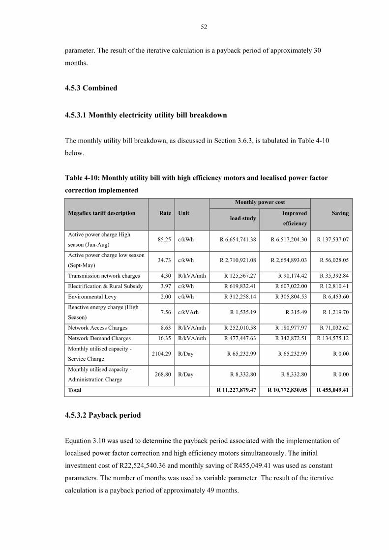
52

parameter. The result of the iterative calculation is a payback period of approximately 30

months.

4.5.3 Combined

4.5.3.1 Monthly electricity utility bill breakdown

The monthly utility bill breakdown, as discussed in Section 3.6.3, is tabulated in Table 4-10

below.

Table 4-10: Monthly utility bill with high efficiency motors and localised power factor

correction implemented

Megaflex tariff description Rate Unit

Monthly power cost

Saving load study

Improved

efficiency

Active power charge High

season (Jun-Aug) 85.25 c/kWh R 6,654,741.38 R 6,517,204.30 R 137,537.07

Active power charge low season

(Sept-May) 34.73 c/kWh R 2,710,921.08 R 2,654,893.03 R 56,028.05

Transmission network charges 4.30 R/kVA/mth R 125,567.27 R 90,174.42 R 35,392.84

Electrification & Rural Subsidy 3.97 c/kWh R 619,832.41 R 607,022.00 R 12,810.41

Environmental Levy 2.00 c/kWh R 312,258.14 R 305,804.53 R 6,453.60

Reactive energy charge (High

Season) 7.56 c/kVArh R 1,535.19 R 315.49 R 1,219.70

Network Access Charges 8.63 R/kVA/mth R 252,010.58 R 180,977.97 R 71,032.62

Network Demand Charges 16.35 R/kVA/mth R 477,447.63 R 342,872.51 R 134,575.12

Monthly utilised capacity -

Service Charge 2104.29 R/Day R 65,232.99 R 65,232.99 R 0.00

Monthly utilised capacity -

Administration Charge 268.80 R/Day R 8,332.80 R 8,332.80 R 0.00

Total R 11,227,879.47 R 10,772,830.05 R 455,049.41

4.5.3.2 Payback period

Equation 3.10 was used to determine the payback period associated with the implementation of

localised power factor correction and high efficiency motors simultaneously. The initial

investment cost of R22,524,540.36 and monthly saving of R455,049.41 was used as constant

parameters. The number of months was used as variable parameter. The result of the iterative

calculation is a payback period of approximately 49 months.

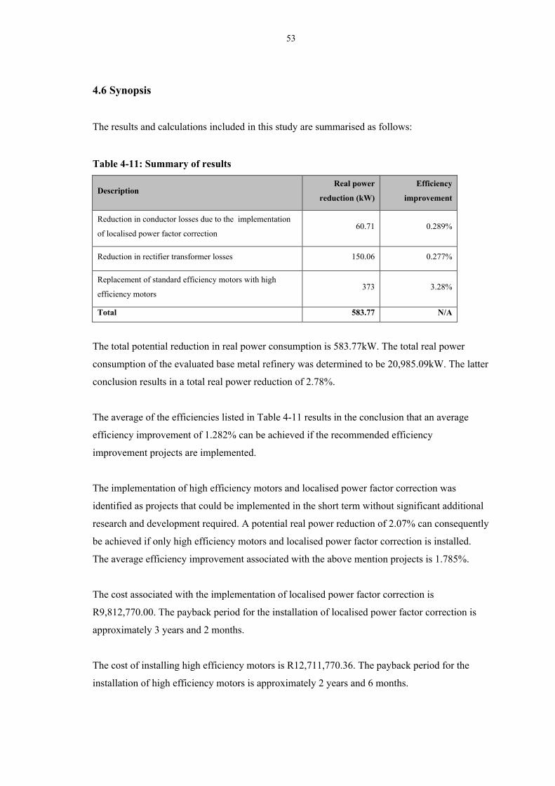
53

4.6 Synopsis

The results and calculations included in this study are summarised as follows:

Table 4-11: Summary of results

Description Real power

reduction (kW)

Efficiency

improvement

Reduction in conductor losses due to the implementation

of localised power factor correction 60.71 0.289%

Reduction in rectifier transformer losses 150.06 0.277%

Replacement of standard efficiency motors with high

efficiency motors 373 3.28%

Total 583.77 N/A

The total potential reduction in real power consumption is 583.77kW. The total real power

consumption of the evaluated base metal refinery was determined to be 20,985.09kW. The latter

conclusion results in a total real power reduction of 2.78%.

The average of the efficiencies listed in Table 4-11 results in the conclusion that an average

efficiency improvement of 1.282% can be achieved if the recommended efficiency

improvement projects are implemented.

The implementation of high efficiency motors and localised power factor correction was

identified as projects that could be implemented in the short term without significant additional

research and development required. A potential real power reduction of 2.07% can consequently

be achieved if only high efficiency motors and localised power factor correction is installed.

The average efficiency improvement associated with the above mention projects is 1.785%.

The cost associated with the implementation of localised power factor correction is

R9,812,770.00. The payback period for the installation of localised power factor correction is

approximately 3 years and 2 months.

The cost of installing high efficiency motors is R12,711,770.36. The payback period for the

installation of high efficiency motors is approximately 2 years and 6 months.

54

The cost associated with the implementation of localised power factor correction as well high

efficiency motors is R22,524,540.36. The monthly electricity utility bill savings associated with

the efficiency improvement projects is R455,049.41. The resultant payback period for the

installation of localised power factor correction as well as high efficiency motors is

approximately 4 years and 1 month.

55

CHAPTER 5: CONCLUSION

A summary of the work, summary of results obtained and suggestion for future work is

discussed in this section.

5.1 Summary of the work

The following list provides a summary of the work done during the project.

A literature review of the technologies as well as efficiencies of a base metal refinery’s

main process areas was conducted.

Power distribution to the various base metal refinery process areas was analysed by

means of a load study. The implemented electro-winning technologies were furthermore

evaluated.

Numerous calculations were performed in order to investigate the efficiency of the

electro-winning and distribution to other areas.

The potential reduction in real power consumption was evaluated as means to improve

efficiency.

The real power reduction was quantified and efficiency improvement projects

recommended.

A financial analysis was performed in order to determine the cost and payback period

associated the implementation of the recommended efficiency improvement projects.

5.2 Summary of results

An evaluation of the load study delivered the first results of this work. A power distribution

breakdown followed the load study. The power distribution breakdown shows that the electro-

winning process contributes 52% of the total base metal refinery apparent power consumption.

The load study furthermore revealed that motor loads contribute 36% of the total apparent

power consumption. The electro-winning area efficiency as well as motor efficiencies therefore

formed the basis of this study.

The efficiency of the rectifier transformers associated with the electro-winning process was

evaluated. The fluctuation in transformer efficiency with winding temperature rise was

identified as an area for potential efficiency improvement and consequently evaluated. An

efficiency improvement of 0.277% can be achieved by limiting the transformer winding

56

temperature rise to 70°C. The total potential reduction in real power consumption summates to

150.06kW for the three transformer sets. Specialised transformer design principles should be

implemented to further evaluate the potential efficiency improvement as well as the consequent

design and manufacturing implications.

The electro-winning area primarily includes rectifiers, rectifier transformers, and an electrolysis

process. The power factor and harmonic distortion produced by the thyristor rectifiers were

evaluated. The introduction of power factor correction filters to the distribution network feeding

the electro-winning process will result in a 27% reduction in apparent power. The real power

requirement for the electro-winning process, however, remains unchanged and therefore does

not offer an efficiency improvement. The increased power factor does, however, realise a

reduction in conductor losses and electricity utility bill cost.

The electro-winning process was evaluated and areas for potential efficiency improvement were

identified. A detailed evaluation of process related efficiency is not included in the scope of this

study. Areas of potential process related efficiency improvement were, however, noted during

this study, discussed and recommended for future evaluation. The influence of stray currents in

the electro-winning process was identified as an area for potential efficiency improvement.

Methods to minimise and monitor stray currents were discussed. The influence of plating

efficiency was identified as another area for potential efficiency improvement. The plating

efficiency of base metals is primarily determined by the electrolyte metal-ion concentration. A

concentrated study of the relevant electrolysis process is required to quantify the potential

improvement in plating efficiency. The influence of busbar losses was identified as an area for

potential efficiency improvement. Busbar losses are mainly determined by the conductor

quality, resistivity and cross sectional area and conductor length. A detailed evaluation of the

specific busbar specification and installation is required to quantify the potential efficiency

improvement of the existing and future busbar installations.

The motor efficiency at the base metal refinery was evaluated. The use of high efficiency

motors as apposed to standard efficiency motors result in an average efficiency improvement of

3.28%. The efficiency improvement results in 373kW reduction in real power consumption

when motors operate at full rated power. Operating motors at reduced voltages when not

operating at full rated power, can compensated for the reduced load and consequently increase

the motor efficiency.

Implementing power factor correction at the satellite substations as apposed to overall power

factor correction at the main consumer substation was evaluated. Implementing power factor

57

correction at the satellite substations will result in a efficiency improvement of 0.289%. The

latter efficiency improvement results in a 60.71kW reduction in conductor losses.

The introduction of a harmonic filter to the local distribution network was evaluated. The

introduction of a harmonic filter results in a potential 25.6% reduction in current THD and a

6.7% potential reduction in voltage THD per rectifier. The potential reduction in THD does not

directly reduce the real power consumption of the rectifiers. The reduction in harmonic content

does, however, result in an improvement in power factor and consequently a reduction in

apparent power consumption. The recommended power factor correction banks can be

expanded to act as harmonic filters as well as power factor correction banks.

The work included in this study reveals that an improvement in power consumption efficiency

is achievable at the evaluated base metal refinery. An average efficiency improvement of

1.785%, realising a reduction in real power consumption of 2.07%, can be achieved by

implementing localised power factor correction and high efficiency motors. An average

efficiency improvement of 1.282% can be achieved with the additional implementation of

specialised, high-efficiency rectifier transformer designs. A total real power reduction of 2.78%

is associated with the 1.282% efficiency improvement.

The implementation of localised power factor correction as well as high efficiency motors was

identified as short term efficiency improvement projects. A financial study was performed to

evaluate the cost associated with the recommended projects. The effect of the reduced power

consumption on the refinery’s monthly electricity utility bill was evaluated. The payback period

for the implementation of the recommended projects was consequently calculated. The

approximate payback period for the implementation of local power factor correction was

calculated to be 3 years and 2 months. The implementation of high efficiency motors will have

an approximate payback period of 2 years and 6 months. The benefit of installing both

recommended efficiency improvement studies simultaneously was furthermore evaluated. A

combined cost of R22,524,540.36 is required to obtain a real power reduction of 2.07%. The

approximate payback period was calculated to be 4 years and 1 month. The implementation of

the efficiency improvement projects as mentioned above is therefore highly recommended

considering that the operating life expectancy of a typical base metal refinery exceeds thirty

years.

58

5.3 Proposals for future work

Further investigation into the specialised field of rectifier transformer efficiency can be

conducted in order to determine further potential efficiency improvement opportunities.

A concentrated analysis of the electro-winning process efficiency can be conducted. Stray

currents, plating efficiency and busbar losses will have an influence on the overall efficiency of

the electro-winning process area.

An efficiency analysis of the other process areas within a base metal refinery can be conducted.

The areas include the milling, autoclave, boiler, heat exchange and filters.

A financial model based on the electricity utility bill and plant wide power consumption can be

developed. The model could be used for cash flow purposes to predict future electricity cost and

to motivate the implementation of efficiency improvement projects.

59

CHAPTER 6: REFERENCES

ABB South Africa [20 August 2008]. Personal communication. Rectifier power factor and

harmonic generation data.

Aberdare [2010]. Cable facts and figures catalogue - Aberdare [Online]. Available from:

http://www.aberdare.co.za/facts-figures [Accessed: 17 November 2010].

Agamloh, E.B., 2009. A Comparison of direct and indirect measurement of induction motor

efficiency. IEEE International Electric Machines and Drives Conference publication. No. 1, 36-

42.

Allwood, J., Ashby, M., Gutowski, T.G., Sahni, S., Worrell, E., 2011. The Energy Required to

Produce Materials: Constraints on Energy Intensity Improvements, Parameters of Demand.

Phylisophical transactions of the Royal Society, pre-publication.

Aqueveque, P.E., Burgos, R.P. and Wiechmann, E.P., 2007. Short-Circuit Detection for

Electrolytic Processes Employing Optibar Intercell Bars. IEEE Transactions on

Hydrometallurgy, 7, 1746-1751.

Anglo American [28 August 2010]. Personal communication. BMR operations philosophy and

power demand data.

Aqueveque, P.E., Wiechmann, E.P. and Burgos, R.P., 2008. On the Efficiency and Reliability of

High-current Rectifiers. IEEE Power Electronics Specialists Conference, 1, 4509.

Baranowski, J.F., Benna, S.J., Bishop, M.T., Heath, D., 1996. Evaluating harmonic-induced

transformer heating. IEEE Transactions on PowerDelivery, 11, 305-311.

Bergh, L., Lo´pez, M., Olivares, M., Pontt, J., Robles, H., Rojas, F., Valderrama, W., Yianatos,

J., 2010. Impact of Process and Energy Efficiency in Mineral Processing on Abatement of

Carbon Emissions. IEEE Industry Applications Society Annual Meeting publication. No. 1, 1 –

7.

60

Bittner, R., Pagliero, A., Salazar, A., Valenzuela, M., 1998. Electric Field And Potential

Determination For Electrowinning Cells with bipolar electrodes by finite difference models.

Industry Applications Conference publication No. 3, 1973-1980.

Blank, L., Tarquin, A., 2002. Engineering Economy. 5th ed. McGraw-Hill Conpanies, Inc.

Boglietti, A., Cavagnino, A., Ferraris, L., Luparia, L.G., 2004. Induction motor efficiency

improvements with low additional production costs. Power Electronics, Machines and Drives

(PEMD 2004) Second International Conference publication No. 2, 775-780.

Braun, M., 1993. Increasing the efficiency of induction motors. Electrical Manufacturing & Coil

Winding Conference publication, No. 1, 41-44.

Breslin, J.G., Hurley, W.G., Wolfle, W.H., 1998. Optimized transformer design: Inclusive of

high-frequency effects. IEEE Transactions on Power Electronics, 13, 651-658.

Capehart, B.L., Kennedy, W.J. and Turner, W.C., 2008. Guide to Energy Management. 6th ed.

The Fairmont Press, Inc.

Castrillon, R., Gonzalez, A.J., Quispe, E.C., 2012. Energy efficiency improvement in the

cement industry through energy management. IEEE Cement Industry Technical Conference

publication, No. 53, 1-13.

Cathey, J.J., 2001. Electric Machines. 1st ed. McGraw-Hill Conpanies, Inc.

Chat-uthai, C., Kedsoi, T., Phumiphak, T., 2005. Energy Management Program for Use of

Induction Motors Based on Efficiency Prediction. IEEE TENCON conference publication, No

1, 1-6.

Crouse, J., Haggerty, N.K., Malone, T.P., 1996. Justifying the use of high efficiency

transformers. IEEE Transactions on Industry Applications, 1, 191-199.

Crouse, J., Haggerty, N.K., Malone, T.P., 1998. Applying high efficiency transformers. IEEE

Transactions on Industry Applications, 4, 50-56.

Damnjanovic, A., Feruson, G., 2004. IEEE Power Engineering Society General Meeting

publication, No. 2, 1416-1419.

61

Eskom [2011]. Eskom Integrated report 2011 - Eskom [Online]. Available from:

http://financialresults.co.za/2011/eskom_ar2011/fact_sheets_11.php

[Accessed: 19 September 2012].

Eskom [2012]. Tariffs and charges brochure 2011/2012 - Eskom [Online]. Available from:

http://www.eskom.co.za/live/click.php?u=%2Fcontent%2FTariffbrochure2011.pdf&o=Item%2

B816&v=f2a201 [Accessed: 23 February 2012].

Groza, V.Z., Pitis, C.D., 2010. Using Global Efficiency Concept in selection decisions of

dedicated equipments. IEEE Electric Power and Energy Conference publication, No. 1, 1-6.

Halliday, D., Resnick, R. and Walker, J., 2001. Fundamentals of Physics. 6th ed. John Wiley &

Sons, Inc.

Indexmundi [2012]. Minerals production statistics per country - Indexmundi [Online]. Available

from: http://www.indexmundi.com/minerals [Accessed: 20 September 2012].

Intex [2007]. Mindoro Nickel Project to be Fast Tracked to Produce 60,000 tonnes Nickel per Year – Intex Resources [Online]. Available from: http://www.intexresources.com/news.cfm?id=21 [Accessed: 22 September 2012]

Kotz, J.C. & Treichel, P., 1999. Chemistry and Chemical Reactivity. 4th ed. Saunders College

Publishing.

Kleingeld, M., Mathews, E. H., Pitis, C. D., van Rensburg, E. H., 2007. A new approach to the

efficiency concept in South African industry. Journal of Energy in South Africa, 18, 51 - 63.

Lan, Z., Li, C., Li, Y., Wang, C., Zhu, C., 2010. IEEE Energy Conversion Congress and

Exposition publication, No. 1, 2087-2090.

Liu, J., Liu, Z., Tai, Y., Yu, H., 2011. Efficiency improvement measures analysis of induction

motors. Electrical Machines and Systems International Conference publication, No. 1, 1-4.

Mineral Information Institute [1998]. MII – Sodium sulphate [Online].

Available from: http://www.mii.org/Minerals/photosodiumsulfate.html [Accessed: 16

December 2008].

62

Mohan, N., Undeland, T.M. and Robbins, W.P., 2003. Power electronics: Converters,

applications, and design. 3rd ed. John Wiley & Sons, Inc.

NERSA [2003]. NRS 48-2: Quality of electricity supply – Rationalised User Specification

[Online]. Available from:

http://www.nersa.org.za/Admin/Document/Editor/file/Electricity/IndustryStandards/NRS048%2

0part%202.pdf [Accessed: 2 October 2008].

Rodriguez, J.R., Pontt, J., Silva, C., Wiechmann, E.P., Hammond, P.W., Santucci, F.W.,

Alvarez, R., Musalem, R., Kouro, S., Lezana, P., 2005. Large current rectifiers: State of the art

and future trends. IEEE Transactions on Industrial Electronics, 53, 738-746.

Scaini, V., Veerkamp, W., 2001. Specifying DC chopper systems for electrochemical

applications. IEEE Transactions on Industrial Applications, 37, 941-948.

Steyn, F., 2011. Efficiency Motors and drives for improving energy efficiency. South African

Energy Efficiency Convention publication, No. 1, 1-7.

WEG [2009]. Low Voltage Motors - IEC General Purpose - Motors - Products & Services -

South Africa - WEG [Online]. Available from: http://www.weg.net/za/Products-

Services/Motors/Low-Voltage-Motors-IEC-General-Purpose [Accessed: 4 July 2009].

Wikipedia [28 May 2008]. Matte (Metallurgy) [Online].

Available from: http://en.wikipedia.org/wiki/Matte_(metallurgy) [Accessed: 16 December

2008].

World Maps [2012]. World Mineral Producer – Maps of World [Online]. Available from:

http://www.mapsofworld.com/minerals/ [Accessed: 20 September 2012].

Yongsug, S., Steimer, P, K., 2009. Application of IGCT in High-Power Rectifiers. IEEE

Transactions on Industrial Applications, 45, 1628 - 1636.