An investigation into mathematical modelling of integrated ... · DYRESM CAEDYM as an aquaculture model for an Integrated Biosystems”, Environmental Biotechnology CRC Annual Conference,

AN INVESTIGATION INTO

MATHEMATICAL MODELLING

OF INTEGRATED BIOSYSTEMS

FOR OPERATIONAL CONTROL

AND MANAGEMENT

By

Khalid Shamim

2014

A Thesis Submitted for the Degree of

Doctor of Philosophy

School of Animal & Veterinary Sciences/

School of Chemical Engineering

The University of Adelaide

Australia

i

ABSTRACT

The South Australian Research & Development Institute (SARDI) and the

Environmental Biotechnology Cooperative Research Centre (EBCRC)

undertook a project “Commercial Scale Integrated Biosystems for Organic

Waste and Wastewater Treatment for the Livestock and Food Processing

Industries”, for which this research forms a part. The Integrated Biosystems

(IBS) project laboratory was set up at the Roseworthy campus of The

University of Adelaide, South Australia. The major objective of this project

was to develop an Integrated Biosystems (IBS) on a commercial scale for

the treatment of wastewater by applying the stages of anaerobic digestion

and bioconversion stages involving algae, zooplankton and fish. The IBS

developed could be used in both rural and urban settings for efficient waste

disposal and generation of energy in the process. The overall aim of this

research was to develop a mathematical model of an IBS for operational

control and management.

The objectives of this research were to:

1. Develop a mathematical model for the anaerobic digestion system.

2. Use an existing model to simulate the aquaculture stages of the IBS

and to test its suitability for a commercial scale IBS for effective

control and management.

3. Conduct a sensitivity analysis on the parameters of the aquaculture

model.

4. Develop an automatic calibration program to validate the

aquaculture model with real time field data.

The major contribution from this research was to elucidate the key

parameters required to simulate the integrated IBS model. The data was

collected through a series of rigorous experimentation for both the anaerobic

digestion and aquaculture modules of the IBS. The data obtained was used

to parameterise a coupled anaerobic digestion-hydrodynamic ecological

ii

model. The resulting model adequately simulated key processes within the

IBS, which was further improved with a novel auto calibration algorithm.

The primary contribution of this work has been to develop an automatic

parameter calibration for the aquaculture component of the model.

Parameter calibration in aquaculture models has been time consuming as it

is basically a “trial and error” procedure. This thesis presents a significant

contribution in this area.

A literature review conducted on the models developed for the IBS and

automatic calibration revealed certain gaps in the previous research

conducted, which formed a basis for further work in this PhD study. A

significant proportion of research time was invested in set up, installation

and commissioning of the pilot plant two-stage anaerobic digestion system

and the Integrated Aquaculture (mesocosm) facility. This was done to

understand the mechanism of the IBS. Both the systems were run for a

period of 12 months for data collection. During this time, operational

glitches and troubleshooting provided the researcher an opportunity to

implement engineering skills in the IBS context and understand the

behaviour of this complex system. Batch scale experiments were conducted

in the laboratory for data collection to develop a model for the anaerobic

digestion system using microbial kinetics. The aquaculture model DYRESM

CAEDYM was used to simulate the aquaculture stages of the IBS. The

model source code was altered to run the model for the IBS set up. Real

time field data could not be obtained as the commercial scale IBS was not

constructed due to administrative hurdles which were beyond the

researcher’s control. A sensitivity analysis was conducted on selected

parameters of the model to determine the behaviour of model outputs on

controlled changes to those parameters. Finally an automatic model

calibration and validation program was written in FORTRAN 90 to

automatically validate the model with field data as opposed to the

conventional methods of manual parameter validation. Pseudo field data

was used for demonstration purposes.

iii

The primary contributions from this research have been to assess the

suitability of DYRESM CAEDYM as the modelling software for the

commercial scale IBS, run a sensitivity analysis on selected parameters of

the model and execute an automatic model calibration and validation

program.

The phytoplankton ponds had a domination of cyanobacteria growth for the

maximum part of the year, due to thermal stratification in the summer

months, which otherwise would not happen in an IBS with proper control

and management. There was negligible zooplankton and fish growth due to

diminished chlorophyte concentrations.

Results from similar IBS studies in India and France were used to compare

results with the proposed commercial IBS. The comparative IBS examples

sourced from sites in India and France show that IBS has been successfully

implemented in different parts of the world comprising tools for better

control and management of ponds. The use of mixing (agitation) and

aeration assist in mixing the ponds and the effluent uniformly which

minimises stratification in ponds and thus reduces the growth of

cyanobacteria, and in turn improves the growth of phytoplankton,

zooplankton and fish. The model DYRESM CAEDYM could incorporate

the use of mixers and aeration in the IBS ponds to overcome the problems

of algal crashes in summer.

The sensitivity analysis conducted on the parameters of the model show that

the model results for phytoplankton growth is highly sensitive to those

parameters that directly affect the growth rates e.g. maximum phytoplankton

growth rate, phytoplankton respiration coefficient and phytoplankton

temperature multiplier. The automated calibration routine incorporated a

novel methodology to calibrate and validate DYRESM CAEDYM

automatically without having to manually adjust parameters. This procedure

is a significant improvement over the conventional methodology of

validating the model by “trial and error” which was time consuming and to a

certain extent inaccurate. The simulations ran successfully to validate the

model parameters with the pseudo field data. This calibration program could

iv

be also used to validate other outputs from the model and is a significant

contribution in this research.

The parameters which can be controlled for managing the commercial scale

IBS in an effective way would be parameters related to inflow and outflow

volumes and flow rates of effluent, retention time of the effluent, nutrient

loads, rates of mixing and aeration within the ponds and control of biomass

conversion for primary, secondary and tertiary productions. These

management strategies could also be used to operate an IBS with a variety

of different effluents to its maximum capacity and construct an IBS with

better module design.

The use of automated calibration of parameters has high applicability in the

development of mathematical models for managing the performance of

wastewater recycling technology, which is in high demand in the modern

world in order to reduce the dependence on limited water resources. The

calibration routine developed in this PhD study has demonstrated that for a

complex aquaculture model like DYRESM CAEDYM where manually

validating the parameters is a tedious task, automatic calibration routine

using GLUE methodology is an effective way to validate the model which

minimises the risks of computational errors.

v

STATEMENT OF ORIGINALITY I certify that this work contains no material which has been accepted for the

award of any other degree or diploma in any university or other tertiary

institution and, to the best of my knowledge and belief, contains no material

previously published or written by another person, except where due

reference has been made in the text. In addition, I certify that no part of this

work will, in the future, be used in a submission for any other degree or

diploma in any university or other tertiary institution without the prior

approval of the University of Adelaide and where applicable, any partner

institution responsible for the joint-award of this degree.

I give consent to this copy of my thesis, when deposited in the University

Library, being made available for loan and photocopying, subject to the

provisions of the Copyright Act 1968.

I also give permission for the digital version of my thesis to be made

available on the web, via the University’s digital research repository, the

Library catalogue and also through web search engines, unless permission

has been granted by the University to restrict access for a period of time.

Signed: ……………………………..

KHALID SHAMIM

Dated: ………………………………

vi

ACKNOWLEDGEMENTS I would like to sincerely thank my Principal Supervisor, Professor Martin S

Kumar and Co-Supervisor, Associate Professor David Lewis for their

continuous support and guidance throughout the entire project. I feel

honoured to have been supervised by these outstanding academics and thank

them for their input, encouragement and undivided attention. I would also

like to thank Environmental Biotechnology Cooperative Research Centre

(EBCRC) for awarding me a full postgraduate scholarship, and in particular

I would like to thank Dr. David Garman for his support and giving me an

opportunity to be part of the Project 6 (P6) group, for which this thesis

forms a part.

I would also like to take this opportunity to thank the many people who

assisted me in my research. Firstly, Dr. Stephen Carr for assisting me in

compiling computer programs and setting up simulations on The University

of Adelaide Server; Mr. Paul Harris for guiding me through the anaerobic

digestion process; Mrs. Sandy Wyatt and Mrs. Belinda Rodda for laboratory

support and Mr. Andrew Ward for helping me understand aquaculture

concepts.

I have also had the privilege to collaborate with several interstate and

overseas researchers that gave invaluable suggestions and scope for

exploration of novel ideas. I would like to express my gratitude to Dr. Matt

Hipsey, Dr. Daniel Botelho and Dr. Jason Antenucci from the Centre for

Water Research, University of Western Australia; Dr. Pratap

Pullammanappallil from University of Florida, USA and Mr. Dennis Trolle

from the University of Waikato, New Zealand

Finally I would like to thank my wife Afreen, my parents and my extended

family for their patience and encouragement throughout my PhD studies.

vii

LIST OF PUBLICATIONS Shamim, K., Kumar, M.S., Lewis, D.M., (2014), “Automated Parameter

Estimation and Calibration”, Hydrological Processes (In review).

Shamim, K., Kumar, M.S., Lewis, D.M., (2008), “Development of

DYRESM CAEDYM as an aquaculture model for an Integrated

Biosystems”, Environmental Biotechnology CRC Annual Conference, 8-10

December 2008, Adelaide, Australia (Poster Presentation).

Shamim, K., Kumar, M.S., Lewis, D.M., (2007), “A mathematical model

for the anaerobic digestion of raw piggery effluent”, 11th World Congress on

Anaerobic Digestion, 23-27 September 2007, Brisbane, Australia (Poster

Presentation).

Shamim, K., Kumar, M.S., Pullammanappallil, P., Ho, G (2006),

“Mathematical model development for anaerobic digestion system in an

Integrated Biosystems”, Environmental Biotechnology CRC Annual

Conference, 28-29 November 2006, Sydney, Australia (Poster Presentation).

viii

Table of Contents

1 Introduction ...................................................................................... 1

1.1 Integrated Biosystems .............................................................................................. 1

1.2 IBS Project ................................................................................................................ 4

1.3 Aim of the Research .................................................................................................. 6

1.4 Background .............................................................................................................. 7

1.5 Commercial Scale Integrated Biosystems .................................................................. 9

1.5.1 Anaerobic Digestion ............................................................................................................. 10 1.5.2 Microalgal Ponds ................................................................................................................. 10 1.5.3 Zooplankton and Fish Ponds ................................................................................................ 11

1.6 Organisation of the Thesis ...................................................................................... 12

1.7 Research Program ................................................................................................... 13

2 Literature Review ............................................................................ 14

2.1 Anaerobic Digestion ............................................................................................... 14

2.1.1 Hydrolysis and Fermentation ............................................................................................... 15 2.1.2 Acetogenesis and Homoacetogenesis ................................................................................. 16 2.1.3 Methanogenesis .................................................................................................................. 16

2.2 Mathematical Models in Anaerobic Digestion ......................................................... 19

2.3 Primary and Secondary Production ......................................................................... 22

2.4 Models developed for Primary and Secondary Production ...................................... 24

2.4.1 The Hydrodynamic Model DYRESM ..................................................................................... 24 2.4.2 The Aquatic Ecological Model CAEDYM ............................................................................... 35

2.5 Techniques used in Water Quality Models Calibration ............................................ 47

2.5.1 GLUE .................................................................................................................................... 49

2.6 Summary ................................................................................................................ 52

3 Experimental Methods and Data Collection ..................................... 54

3.1 Introduction ........................................................................................................... 54

3.2 Set up of the Pilot Scale Two-‐Stage Anaerobic Digestion System ............................. 55

ix

3.2.1 Equipment: Reactors and Digesters ..................................................................................... 55 3.2.2 Analytical techniques ........................................................................................................... 57

3.3 Pilot Plant Stage 1 Experiments .............................................................................. 59

3.3.1 Acidogenesis ........................................................................................................................ 59 3.3.2 Methanogenesis .................................................................................................................. 59 3.3.3 Results ................................................................................................................................. 60

3.4 Pilot Plant Stage 2 Experiments .............................................................................. 65

3.4.1 Methods ............................................................................................................................... 65 3.4.2 Results ................................................................................................................................. 67 3.4.3 Conclusions .......................................................................................................................... 80

3.5 Set up of the Pilot Scale Integrated Aquaculture System ......................................... 82

3.6 Bioconversion of piggery effluent to algae (280 L working volume) ......................... 84

3.6.1 Objective .............................................................................................................................. 84 3.6.2 Materials and Methods ....................................................................................................... 84 3.6.3 Results ................................................................................................................................. 85 3.6.4 Key findings .......................................................................................................................... 88

3.7 Bioconversion of piggery effluent to algae (180 L working volume) ......................... 88

3.7.1 Objective .............................................................................................................................. 88 3.7.2 Materials and Methods ....................................................................................................... 89 3.7.3 Results ................................................................................................................................. 89 3.7.4 Key findings .......................................................................................................................... 92

3.8 Lab Scale Anaerobic Digestion Experiments ............................................................ 93

3.8.1 Introduction ......................................................................................................................... 93 3.8.2 Materials & Methods ........................................................................................................... 93

3.9 Conclusions ............................................................................................................ 95

4 Development of an Anaerobic Digestion Model ............................... 97

4.1 Introduction ........................................................................................................... 97

4.2 Methods ................................................................................................................. 98

4.2.1 Development of Model Equations for the Anaerobic Digestion Process ........................... 101

4.3 Results .................................................................................................................. 103

4.3.1 Methane Model ................................................................................................................. 103 4.3.2 TAN Model ......................................................................................................................... 105 4.3.3 P Model .............................................................................................................................. 107

x

4.4 Comparison of model data vs. measured data ...................................................... 108

4.5 Discussion ............................................................................................................. 112

4.6 Further Work ........................................................................................................ 113

5 Modelling Commercial Scale Integrated Biosystems ...................... 115

5.1 Introduction ......................................................................................................... 115

5.1.1 Model Description ............................................................................................................. 117

5.2 Methods ............................................................................................................... 118

5.2.1 Research Site ..................................................................................................................... 118 5.2.2 Alterations to the original source code of DYRESM CAEDYM ............................................ 119 5.2.3 Input Data .......................................................................................................................... 121

5.3 Results .................................................................................................................. 125

5.3.1 Temperature ...................................................................................................................... 125 5.3.2 Phytoplankton growth in algal pond 1 ............................................................................... 126 5.3.3 Phytoplankton growth in algal pond 2 ............................................................................... 130 5.3.4 Zooplankton growth .......................................................................................................... 134 5.3.5 Fish growth ........................................................................................................................ 136

5.4 Discussion ............................................................................................................. 139

5.4.1 Limitations of the model .................................................................................................... 142 5.4.2 Comparison with algal data obtained from Bolivar Wastewater Treatment Plant ........... 143

5.5 Typical Outputs from established IBS .................................................................... 145

5.5.1 Central Institute of Freshwater Aquaculture, India ........................................................... 145 5.5.2 IBS set up in France ............................................................................................................ 147

5.6 Conclusions .......................................................................................................... 149

6 Sensitivity Analysis ........................................................................ 152

6.1 Introduction ......................................................................................................... 152

6.2 Methods ............................................................................................................... 154

6.3 Results .................................................................................................................. 157

6.3.1 Maximum Phytoplankton Growth Rate (Pmax) ................................................................... 157 6.3.2 Phytoplankton Respiration Coefficient (kr) ........................................................................ 158 6.3.3 Phytoplankton Temperature Multiplier (vR) ...................................................................... 159 6.3.4 Minimum Phytoplankton Internal P (IPmin) ........................................................................ 160 6.3.5 Maximum Phytoplankton Internal P (IPmax) ....................................................................... 161

xi

6.3.6 Maximum Rate of Phytoplankton P Uptake (UPmax) .......................................................... 162 6.3.7 Minimum Phytoplankton Internal N (INmin) ....................................................................... 163 6.3.8 Maximum Phytoplankton Internal N (INmax) ...................................................................... 164 6.3.9 Maximum Rate of Phytoplankton N Uptake (UNmax) ......................................................... 165 6.3.10 Half Saturation Constant for Phytoplankton P Uptake (KP) ............................................. 166 6.3.11 Half Saturation Constant for Phytoplankton N Uptake (KN) ............................................ 167 6.3.12 Parameter for initial slope of P-‐I curve (Ik) ...................................................................... 168

6.4 Discussion ............................................................................................................. 169

6.5 Conclusions and Further Work .............................................................................. 171

7 Automated Parameter Estimation and Calibration ........................ 172

7.1 Introduction ......................................................................................................... 172

7.2 Methods ............................................................................................................... 173

7.2.1 Incorporating Monte Carlo and GLUE calibration in DYRESM CAEDYM ............................ 173 7.2.2 Analysis of the auto calibration program .......................................................................... 174 7.2.3 Flowchart of the GLUE program ........................................................................................ 176

7.3 Results .................................................................................................................. 177

7.3.1 GLUE Calibration for Chlorophyte growth ......................................................................... 177 7.3.2 GLUE calibration for Cyanobacteria growth ...................................................................... 181

7.4 Discussion and Conclusions ................................................................................... 184

7.5 Further Work ........................................................................................................ 186

8 Summary and Conclusions ............................................................. 187

8.1 General Discussions and Conclusions .................................................................... 187

8.2 Summary of the Research Results ......................................................................... 187

8.2.1 Laboratory Experiments and Development of Anaerobic Digestion Model ...................... 187 8.2.2 Modelling the Aquaculture Component of the IBS ............................................................ 189 8.2.3 Sensitivity Analysis ............................................................................................................. 191 8.2.4 Automated Parameter Estimation and Calibration ........................................................... 191

8.3 Summary .............................................................................................................. 192

8.4 Recommendations for further studies .................................................................. 192

9 References ..................................................................................... 195

xii

Appendix A Anaerobic Digestion Models .......................................... 219

Appendix B Data from Batch Scale Anaerobic Digestion

Experiments 229

Appendix C DYRESM CAEDYM INPUT FILES ....................................... 233

Appendix D Nutrient Data in the IBS ponds ....................................... 235

Appendix E Program Code for Auto Calibration of DYRESM

CAEDYM 250

Appendix F GLUE Calibration Numerical Outputs .............................. 260

xiii

Table of Figures Figure 1.1 Schematic of material flow within an Integrated Biosystems ............... 3

Figure 1.2 Schematic of the IBS Project ................................................................. 5

Figure 1.3 Flowchart of the IBS process ............................................................... 11

Figure 2.1 Flow Chart of processes in anaerobic digestion

(Pullammanappallil, Chynoweth et al. 2001) ........................................................ 18

Figure 2.2 Schematic Flow Chart of DYRESM (Robson and Hamilton

2004) ...................................................................................................................... 25

Figure 2.3 DYRESM simulation process (Imerito 2007) ..................................... 26

Figure 2.4 Surface energy flux exchanges ............................................................ 29

Figure 2.5 Overview of CAEDYM state variables showing the water

column, benthic and sediment components (Hipsey, Romero et al. 2006) ........... 36

Figure 2.6 Schematic of phytoplankton dynamics within CAEDYM

(Hipsey, Romero et al. 2006) ................................................................................ 38

Figure 2.7 Schematic of zooplankton dynamics within CAEDYM (Hipsey,

Romero et al. 2006) ............................................................................................... 42

Figure 2.8 Schematic of fish dynamics within CAEDYM (Hipsey, Romero

et al. 2006) ............................................................................................................. 46

Figure 3.1 Schematic diagram of the pilot scale anaerobic digestion system ....... 57

Figure 3.2 Thermophilic (stainless steel) digesters in the pilot scale research

facility .................................................................................................................... 58

Figure 3.3 Mesophilic (polybag) digesters in the pilot scale research facility ...... 58

Figure 3.4 pH profile during acidogenesis in T1 and T2 treating piggery

effluent .................................................................................................................. 61

Figure 3.5 Ammonia (TAN) levels in T1 and T2 during acidification of raw

piggery effluent ..................................................................................................... 62

Figure 3.6 Soluble Phosphorus (SP) levels in T1 and T2 during the

acidification of raw piggery effluent ..................................................................... 62

Figure 3.7 Gas production during anaerobic acidification of piggery effluent

in T1 (55 0C) and T2 (38 0C) ................................................................................. 63

Figure 3.8 Gas production during anaerobic digestion of acidified piggery

effluent in polydigesters 1 and 2 operating under ambient conditions .................. 65

xiv

Figure 3.9 pH profile during acidogenesis in reactors T1 and T2 treating raw

piggery effluent ..................................................................................................... 71

Figure 3.10 VFA profile during acidogenesis in reactors T1 and T2 treating

raw piggery effluent .............................................................................................. 72

Figure 3.11 TKN profile during acidogenesis in reactors T1 and T2 treating


Figure 3.12 Ammonia nitrogen profile during acidogenesis in reactors T1

and T2 treating raw piggery effluent ..................................................................... 73

Figure 3.13 TP profile during acidogenesis in reactors T1 and T2 treating


Figure 3.14 SP profile during acidogenesis in reactors T1 and T2 treating


Figure 3.15 Biogas production and methane composition during

acidogenesis in reactors T1 and T2 treating raw piggery effluent ........................ 74

Figure 3.16 pH profile during anaerobic digestion in polydigesters D1, D2,

D3 & D4 treating acidified piggery effluent from the acidogenic reactors ........... 77

Figure 3.17 VFA profile during anaerobic digestion in polydigesters D1,

D2, D3 & D4 treating acidified piggery effluent from the acidogenic

reactors .................................................................................................................. 78

Figure 3.18 TKN profile during digestion in polydigesters D1, D2, D3 & D4

treating acidified piggery effluent from the acidogenic reactors .......................... 78

Figure 3.19 Ammonia profile during digestion in polydigesters D1, D2, D3

& D4 treating acidified piggery effluent from the acidogenic reactors ................ 79

Figure 3.20 Soluble P profile during digestion in polydigesters D1, D2, D3

& D4 treating acidified piggery effluent from the acidogenic reactors ................ 79

Figure 3.21 Biogas production and methane composition during digestion in

polydigesters D1, D2, D3 & D4 treating acidified piggery effluent from the

acidogenic reactors ................................................................................................ 80

Figure 3.22 Schematic diagram of the pilot scale Integrated Aquaculture

System ................................................................................................................... 83

Figure 3.23 Clear Perspex tanks set up at differential heights for micro-algal

culture while blue fibre glass tanks are used for fish culture. These tanks are

part of the indoor integrated aquaculture system (mesocosm) at Roseworthy

Laboratory ............................................................................................................. 83

xv

Figure 3.24 Mean cell density in 280 L algal culture ............................................ 86

Figure 3.25 Mean TAN concentration in 280 L algal culture ............................... 87

Figure 3.26 Mean SP concentration in 280 L algal culture ................................... 87

Figure 3.27 Mean pH in 280 L algal culture ......................................................... 88

Figure 3.28 Mean cell density for 180 L algal culture .......................................... 90

Figure 3.29 Mean TAN for 180 L algal culture .................................................... 91

Figure 3.30 Mean SP for 180 L algal culture ........................................................ 91

Figure 3.31 Mean pH for 180 L algal culture ........................................................ 92

Figure 3.32 Experimental apparatus for the laboratory study of anaerobic

digestion. ............................................................................................................... 95

Figure 4.1 Decrease in COD of the raw piggery effluent ..................................... 98

Figure 4.2 Cumulative methane output ................................................................. 99

Figure 4.3 Increase in TAN of the raw piggery effluent ....................................... 99

Figure 4.4 Increase in soluble P of the raw piggery effluent .............................. 100

Figure 4.5 Scaled/Normalized Plot for Anaerobic Digestion of Piggery

Effluent ................................................................................................................ 101

Figure 4.6 Modelled methane data at 55 0C ........................................................ 104

Figure 4.7 Temperature Response for Growth and Death Rates in CH4

modelling ............................................................................................................. 105

Figure 4.8 Modelled Total Ammonia Nitrogen (TAN) data at 55 0C ................. 106

Figure 4.9 Temperature Response for Growth and Death Rates in TAN

modelling ............................................................................................................. 106

Figure 4.10 Modelled Soluble P data at 55 0C .................................................... 107

Figure 4.11 Temperature Response for Growth and Death Rates in P

modelling ............................................................................................................. 108

Figure 5.1 Schematic of the proposed commercial scale IBS ............................. 119

Figure 5.2 Meteorological data comprising short wave radiation, air

temperature, rainfall, wind speed, cloud cover and vapour pressure

(clockwise, starting from left) ............................................................................. 123

Figure 5.3 Simulated pond temperature (all ponds are the same

temperature) ........................................................................................................ 125

Figure 5.4 Simulated chlorophyte growth in algal pond 1 .................................. 126

Figure 5.5 Simulated cyanobacteria growth in algal pond 1 ............................... 127

Figure 5.6 Simulated freshwater diatoms growth in algal pond 1 ....................... 128

xvi

Figure 5.7 Nutrient Profile in Algal Pond 1 ........................................................ 129

Figure 5.8 Simulated chlorophyte growth in algal pond 2 .................................. 130

Figure 5.9 Simulated cyanobacteria growth in algal pond 2 ............................... 131

Figure 5.10 Simulated fresh water diatoms growth in algal pond 2 .................... 132

Figure 5.11 Nutrient Profile in Algal Pond 2 ...................................................... 133

Figure 5.12 Simulated zooplankton growth in zooplankton pond ...................... 134

Figure 5.13 Nutrient Profile in Zooplankton Pond ............................................. 135

Figure 5.14 Simulated fish growth in fish pond .................................................. 136

Figure 5.15 Simulated zooplankton growth in fish pond .................................... 137

Figure 5.16 Nutrient Profile in Fish Pond ........................................................... 138

Figure 5.17 Algal succession data obtained from Bolivar Wastewater

Treatment Plant ................................................................................................... 144


Treatment Plant for the period 2000 - 2001 ........................................................ 144

Figure 5.19 Diagram of the pilot-scale IBS for recycling swine manure in

France .................................................................................................................. 149

Figure 6.1 Chlorophyll-a response to change in Pmax values .............................. 157

Figure 6.2 Chlorophyll-a response to change in kr values .................................. 158

Figure 6.3 Chlorophyll-a response to change in vR values .................................. 159

Figure 6.4 Chlorophyll-a response to changes in IPmin values ............................ 160

Figure 6.5 Chlorophyll-a response to changes in IPmax values ............................ 161

Figure 6.6 Chlorophyll-a response to changes in UPmax values .......................... 162

Figure 6.7 Chlorophyll-a response to changes in INmin values ........................... 163

Figure 6.8 Chlorophyll-a response to changes in INmax values ........................... 164

Figure 6.9 Chlorophyll-a response to changes in UNmax values ......................... 165

Figure 6.10 Chlorophyll-a response to changes in KP values ............................. 166

Figure 6.11 Chlorophyll-a response to changes in KN values ............................. 167

Figure 6.12 Chlorophyll-a response to changes in Ik values ............................... 168

Figure 7.1 FlowChart of the Monte Carlo & GLUE Calibration script .............. 176

Figure 7.2 Nash Sutcliffe Coefficients for GLUE Calibration ............................ 177

Figure 7.3 Comparison between simulated (model) and field data before

GLUE calibration for chlorophyte growth .......................................................... 179

Figure 7.4 Comparison between simulated (model) and field data after

GLUE calibration for chlorophyte growth .......................................................... 179

xvii

Figure 7.5 Nash – Sutcliffe Coefficients for GLUE calibration for

cyanobacteria growth .......................................................................................... 181


GLUE calibration for cyanobacteria growth ....................................................... 183


GLUE calibration for cyanobacteria growth ....................................................... 183

xviii

List of Tables

Table 2.1 Description of the seven phytoplankton groups configurable

within CAEDYM .................................................................................................. 37

Table 3.1 Effluent characteristics in T1 and T2 .................................................... 60

Table 3.2 Effluent characteristics in the polydigesters operating at ambient

temperature ............................................................................................................ 64

Table 3.3 Performance parameters of acidogenic reactor T1 (38 0C) during

period 1 (Days 1-65) ............................................................................................. 67


period 1 (Days 1-65) ............................................................................................. 67


period 2 (Day 65-112) ........................................................................................... 69


period 2 (Day 65-112) ........................................................................................... 70

Table 3.7 Performance parameters of Polydigesters D1 and D3 (ambient

temperature) during Period 1 (Days 1-65) ............................................................ 75


temperature) during Period 1 (Days 1-65) ............................................................ 75


temperature) during Period 2 (Days 65-112) ....................................................... 76

Table 3.10 Performance parameters of polydigesters D2 and D4 (ambient

temperature) during period 2 (Days 65-112) ......................................................... 76

Table 3.11 Comparison of data between experiments 1 and 2 .............................. 92

Table 3.12 Characteristics of the raw piggery effluent from the Roseworthy

piggery ................................................................................................................... 93

Table 3.13 Characteristics of the raw piggery effluent data .................................. 94

Table 3.14 Data from experiments to be used in IBS model development ........... 96

Table 4.1 Fitted r2 values for CH4 ....................................................................... 103

Table 4.2 Refitted Growth and Death Rates for CH4 with r2 values ................... 103

Table 4.3 Fitted r2 values for TAN ...................................................................... 105

Table 4.4 Refitted Growth and Death Rates for TAN with r2 values .................. 105

Table 4.5 Fitted r2 values for Soluble P .............................................................. 107

xix

Table 4.6 Refitted Growth and Death Rates for Soluble P with r2 values .......... 107

Table 4.7 Comparison of modelled CH4 and measured CH4 data ....................... 109

Table 4.8 Comparison of modelled TAN and measured TAN data .................... 110

Table 4.9 Comparison of modelled P and measured P data ................................ 111

Table 5.1 Nutrient Concentrations in different stages of the IBS ....................... 141

Table 5.2 Nutrient and Plankton outputs from Central Institute of

Freshwater Aquaculture system .......................................................................... 146

Table 6.1 Parameters used in sensitivity analysis (Schladow and Hamilton

1997) .................................................................................................................... 155

Table 6.2 Parameters used in the sensitivity analysis study ................................ 156

Table 6.3 Comparison of percentage variation in input parameter and output

Chl-a .................................................................................................................... 170

Table 7.1 GLUE Calibration results for 10 random simulations ........................ 178

Table 7.2 Numerical Values of the Calibrated Parameters ................................. 180

Table 7.3 GLUE Calibration Results for 10 random simulations ....................... 182

Table 7.4 Numerical Values of the Calibrated Parameters ................................. 184

1

1 Introduction

1.1 Integrated Biosystems

Integrated Biosystems (IBS) connect different food production activities

with other operations such as waste treatment and fuel generation

(Warburton, Ramage et al. 2002). An Integrated Biosystem is a continuous

closed loop or open system comprising of production and consumption

where outputs from one operation become inputs to another. This enables

the reuse of resources and minimises environmental impact.

“Integrare” is a latin verb which means to make whole and to complete by

adding parts or to combine parts into a whole. The concept of IBS is not

new. There has been evidence found on an ancient Egyptian painting of

about 2000B.C. that seems to present an IBS for pond aquaculture where

nutrients in the pond water were used to cultivate flowers, vegetables and

fruits. Other early civilisations, such as those in China and Mexico have also

developed integrated farming systems that are unique to their regions. IBS is

widely practised in China today for the production of food, fuel and

aquaculture species (Zhang 1990).

Examples of different kinds of IBS are described below (Warburton,

Ramage et al. 2002):

1. Simple systems: e.g. livestock manure used directly as a fertiliser in

agriculture.

2. Intermediate systems: e.g. organic waste → compost → agriculture.

3. Closed systems: e.g. livestock manure → fodder crop → feed

→livestock.

4. Fuel generation: e.g. organic waste → biogas.

5. Nutrient stripping and bioconversion: e.g. wastewater effluent from

sewage treatment or livestock is stored into lagoons and used to grow

floating aquatic plants (e.g. duckweed). Duckweed consumes the

nutrients from the effluent and in turn reduces the high nutrient load to a

2

level where the water can be used for crop irrigation. The duckweed is

also harvested and used as feed for livestock and fish.

6. Water reuse: e.g. recycling dams allow the same water to be used for

growing several crops.

7. Industrial by-products: e.g. fermentation of grain (to produce beer,

spirits, biofuels) produces organic residues, heat and carbon dioxide.

The organic residues can be used in aquaculture to increase the

production of cultured fish, the carbon dioxide can be used for aerated

drink production, and both heat and carbon dioxide can be used as a

catalyst to improve growing conditions in hydroponic greenhouses.

8. Settlements: e.g. integration of waste treatment systems with housing

(septic tanks).

The IBS concept consists of three basic principles:

1. Use all the available wastes and organic materials instead of discarding

them.

2. Obtain at least one or more valuable products from the wastes.

3. Develop a closed loop continuous system using organisms through

biological processes for nutrient and wastewater recycling so that the

resources are completely utilised and there is no waste disposal.

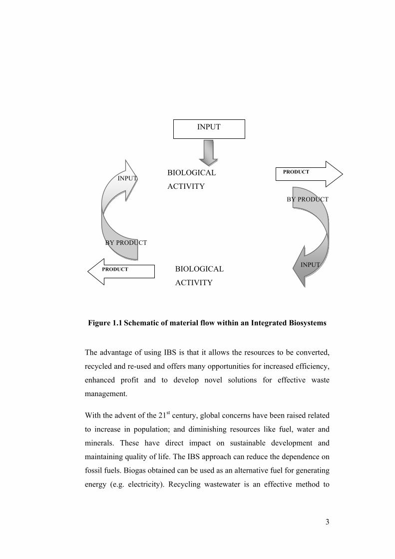
The nutrient and material flows within an IBS are shown in Figure 1.1

summarising the IBS concept discussed previously. The input which is

essentially wastewater effluent enters the IBS process where it is subject to

a first biological process (e.g. microbial activity). As a result of this, a

product and by product are formed. The by product is used as an input to the

subsequent biological process. After the second biological process, a

product and by product are formed. The by product can be recycled back

into the first biological process thus completing a continuous cycle or it can

flow on to further biological processes before completing the loop. At each

stage the product formed can be put to effective use (e.g. energy generation

etc).

3

Figure 1.1 Schematic of material flow within an Integrated Biosystems

The advantage of using IBS is that it allows the resources to be converted,

recycled and re-used and offers many opportunities for increased efficiency,

enhanced profit and to develop novel solutions for effective waste

management.

With the advent of the 21st century, global concerns have been raised related

to increase in population; and diminishing resources like fuel, water and

minerals. These have direct impact on sustainable development and

maintaining quality of life. The IBS approach can reduce the dependence on

fossil fuels. Biogas obtained can be used as an alternative fuel for generating

energy (e.g. electricity). Recycling wastewater is an effective method to

BIOLOGICAL

ACTIVITY

BIOLOGICAL

ACTIVITY

INPUT

PRODUCT

PRODUCT

INPUT

BY PRODUCT

BY PRODUCT

INPUT

4

reuse dwindling water resources and utilise it in aquaculture, agriculture and

horticulture for the benefit of everyone.

The IBS should be flexible enough to be used by both an ordinary farmer

for simple agricultural systems or by a large scale processing industry for

complex systems (e.g. abattoir, winery waste treatment) (Warburton 2001).

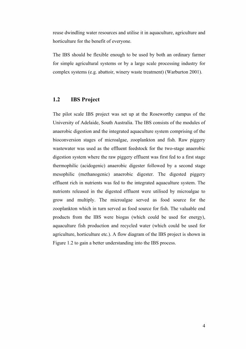
1.2 IBS Project

The pilot scale IBS project was set up at the Roseworthy campus of the

University of Adelaide, South Australia. The IBS consists of the modules of

anaerobic digestion and the integrated aquaculture system comprising of the

bioconversion stages of microalgae, zooplankton and fish. Raw piggery

wastewater was used as the effluent feedstock for the two-stage anaerobic

digestion system where the raw piggery effluent was first fed to a first stage

thermophilic (acidogenic) anaerobic digester followed by a second stage

mesophilic (methanogenic) anaerobic digester. The digested piggery

effluent rich in nutrients was fed to the integrated aquaculture system. The

nutrients released in the digested effluent were utilised by microalgae to

grow and multiply. The microalgae served as food source for the

zooplankton which in turn served as food source for fish. The valuable end

products from the IBS were biogas (which could be used for energy),

aquaculture fish production and recycled water (which could be used for

agriculture, horticulture etc.). A flow diagram of the IBS project is shown in

Figure 1.2 to gain a better understanding into the IBS process.

5

Figure 1.2 Schematic of the IBS Project

LIVESTOCK

(ORGANIC

WASTE)

RECYCLED

WATER

THERMOPHILIC

ANAEROBIC DIGESTION

MESOPHILIC ANAEROBIC

DIGESTION

MICROALGAE

ZOOPLANKTON FISH

BIOGAS

6

1.3 Aim of the Research

The aim of this research was to develop a mathematical model for

Integrated Biosystems (IBS) which could be used as a tool for operational

management and process control and to also investigate the suitability of

aquaculture model DYRESM CAEDYM for modelling an IBS. Previous

modelling studies on IBS have been restricted to modelling the individual

IBS units rather than the whole system.

The major contribution from this research was to elucidate the key

parameters required to simulate the integrated IBS model. The data was

collected through a series of rigorous experimentation for both the anaerobic

digestion and aquaculture modules of the IBS. The data obtained was used

to parameterise a coupled anaerobic digestion-hydrodynamic ecological

model. The resulting model adequately simulated key processes within the

IBS, which was further improved with a novel auto calibration algorithm.

The primary contribution of this work has been to develop an automatic

parameter calibration for the aquaculture component of the model.

Parameter calibration in aquaculture models has been time consuming as it

is basically a “trial and error” procedure. This thesis presents a significant

contribution in this area.

Summarising, the objectives of this PhD research are to

1) Develop a mathematical model for the anaerobic digestion system

using microbial kinetics. The outputs of this model can be used as an

input to the aquaculture model.

2) Use DYRESM CAEDYM as an existing model to test its suitability

for modelling the aquaculture component of the IBS comprising of

bioconversion stages of algae, zooplankton and fish. This model will

be modified to suit the operating conditions and dimensions

(morphometry) of the IBS.

3) Conduct a sensitivity analysis on the modified DYRESM CAEDYM

aquaculture model.

7

4) Develop a computer program for automated calibration and

parameter estimation for the aquaculture model.

1.4 Background

The 21st century has exhibited global concerns related to increasing

population, diminishing fossil energy, water, land resources and higher

levels of pollution. These have multiple effects on sustainable development

and maintaining the quality of life in the future. The IBS approach can

reduce the need for fossil fuel. Biogas technology will play a unique role as

it provides energy, nutrients and better sanitation. Large volumes of biogas

can provide electricity to the grid, local communities and industries

(Mansson 1998; Kranert M. 2000).

Wastewater (effluent) from livestock is not a pollutant necessarily but a

nutrient source which can be recycled. There through integrated farming

practices has been evidence of recycling effluent through agriculture,

horticulture and aquaculture in several Asian countries (Kumar and Crips

2012). Aquaculture is common in many developing countries and has been

adapted as a technology for treatment of wastewater (Islam 1996). Examples

are sewage fed fish culture in Munich, Germany and the “bheries” in

Kolkata, India (Kumar 2002). Integrated farming systems with aquaculture

as a module differ from the traditional extensive and intensive farming

systems as aquaculture is used as a tool for recycling wastewater and

recovering nutrients.

A major concern in the 21st century is environmental pollution from solid

wastes and wastewaters from mega-cities, intensive animal farms and

industries. The ‘waste’ which provides income through producing a

valuable product, in effect, becomes a ‘resource’ (Crips and Kumar 2003).

Nitrogen (N) and phosphorus (P) are resources and their bioavailability can

be optimised through aerobic or anaerobic digestion processes. The process

simply allows recycling the nutrient and water, prevents aquatic pollution

8

and produces valuable end products. The IBS approach can have a

multipurpose role in sustainable environmental protection as it cleans the

environment and can generate products of economic value at the same time.

The amount of wastewater generated has been increasing over the years

with the increase in human population. Large amounts of domestic sewage,

industrial effluents and solid wastes are being generated everyday which has

made treatment difficult. There are different processes of wastewater

treatment e.g. conventional activated sludge and trickling filter methods,

oxidation/waste stabilisation ponds, aerated lagoons and variation in

anaerobic treatment systems (Gopakumar, Ayyappan et al. 2000). However

while most of these are energy-based treatment processes, only a few of

them lead to any resource recovery e.g. root zone treatment, wetland system,

aquatic macrophyte and aquaculture. Knowledge of macrophytes being used

as an effective agent for removing nutrients from wastewater led to the

concept of treatment of domestic sewage through aquaculture. A more

developed process called the Up Flow Anaerobic Sludge Blanket (UASB)

has also been developed (Pearson 1987; Curtis 1992; Pearson 1996).

Wastewater treatment usually involves additional costs (e.g. energy usage).

If the treatment itself produces income, prevents pollution and complies

with the environmental standards, it increases the profitability and the

sustainability of the industry (Williams, Biswas et al. 2007). While treating

the organic waste in the sewage, aquaculture products (fish), aquatic plants

and agricultural products can be produced. The introduction of aquaculture

into the wastewater treatment industry to remove nutrients and release clean

effluent has proved to be successful in many different countries (Edwards

and Pullin 1990). Some examples of these are

• Pig-biogas-duckweed-cassava IBS in Vietnam

• Brewery wastes-duck-insect larvae-aquatic plants-earthworm IBS in

Samoa

• Compost toilet and graywater garden system in Fiji

• St. Petersburg Eco-House, Russia

• Pozo Verde Farm in Colombia

9

• Sewage-duckweed-fish-banana IBS in Bangladesh

• Rice-flower-fish IBS in China

1.5 Commercial Scale Integrated Biosystems

The uniqueness of an IBS is that it is capable of handling large volumes of

wastewater from a variety of industries. Wastewater treatment in an IBS

could be through a series of biological processes complementing each other.

In 2005, the South Australian Research & Development Institute (SARDI)

and the Environmental Biotechnology Cooperative Research Centre

(EBCRC) commenced a project, entitled “Commercial scale integrated

biosystems for organic waste and wastewater treatment for the livestock and

food processing industries”, for which this research forms a part. This

project was proposed to be set up at Roseworthy Campus, The University of

Adelaide, where there is a commercial pig and poultry unit, and

considerable land available.

Raw piggery effluent was chosen as the source of wastewater which is

available from the Roseworthy piggery. Pigs have a high efficiency of food

conversion and are capable of reproducing and sustaining themselves by

feeding on farm wastes and kitchen refuse (Gopakumar, Ayyappan et al.

2000). Pig waste has certain advantages over cow, horse, sheep and goat

waste for aquaculture because pigs have a limited capability to consume

roughage. As a result their excreta contain lesser amounts of cellulose,

hemicellulose and lignin which are difficult to decompose, as these

materials are not a large part of the feed mix for pigs (Flachowsky and

Hennig 1990). These organic compounds form a blanket at the bottom of the

pond, which becomes a maintenance problem. The waste produced by 20–

30 pigs per year is equivalent to 1 tonne of ammonium sulphate supplied to

the soil (Kumar and Sierp 2003).

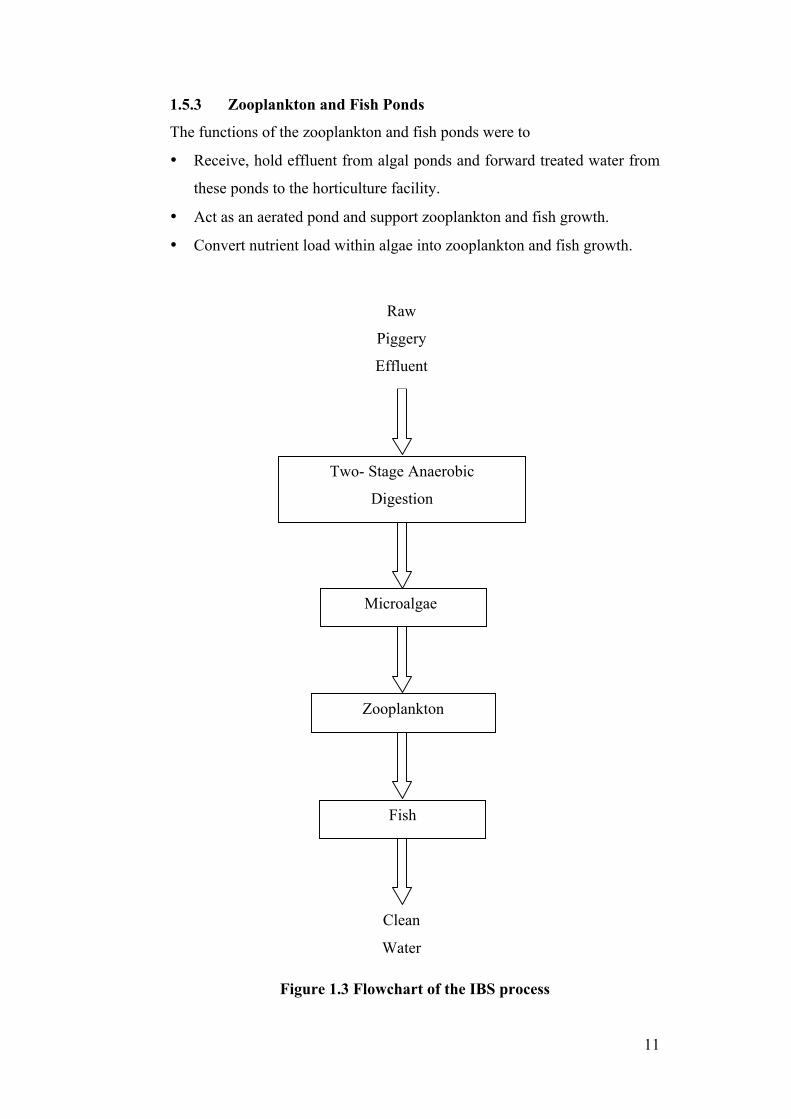
The treatment of raw piggery effluent is planned through the following

stages of an IBS as shown in Figure 1.3.

10

1.5.1 Anaerobic Digestion

Anaerobic digestion of the raw piggery effluent is proposed to be conducted

in two stages. A primary thermophilic treatment conducted at 500 C

acidifies the raw piggery effluent. The purpose of this stage is to kill the

pathogens present. A secondary mesophilic treatment conducted at ambient

temperature generates methane rich biogas and effluent rich in nitrogen (N)

and phosphorus (P) which is in bio available forms to be utilised in culturing

micro algae, zooplankton and fish downstream.

The functions of the anaerobic digesters within the IBS project were to

• Receive, hold and anaerobically digest piggery effluent received from

storage sump;

• Generate biogas rich in methane during the anaerobic digestion process;

• Produce nutrients (N & P) in bioavailable form to be used in subsequent

aquaculture stages of the IBS downstream. N will be present in the form

of total ammonia nitrogen (TAN) (approximately 80% of total nitrogen,

TN) and P will be present in the form of soluble phosphorus (SP)

(approximately 70% of total phosphorus).

1.5.2 Microalgal Ponds

The functions of the algal ponds are to

• Receive and hold effluent from anaerobic digesters and reduce

concentrations of nutrients (N & P) by algal growth.

• Maximise algal growth.

11

1.5.3 Zooplankton and Fish Ponds

The functions of the zooplankton and fish ponds were to

• Receive, hold effluent from algal ponds and forward treated water from

these ponds to the horticulture facility.

• Act as an aerated pond and support zooplankton and fish growth.

• Convert nutrient load within algae into zooplankton and fish growth.

Figure 1.3 Flowchart of the IBS process

Raw

Piggery

Effluent

Two- Stage Anaerobic

Digestion

Microalgae

Zooplankton

Fish

Clean

Water

Raw

Piggery

Effluent

12

1.6 Organisation of the Thesis

A literature review is presented in Chapter 2 which describes different

mathematical models developed for both anaerobic digestion and

aquaculture systems. Chapter 2 provides background knowledge and

presents the research required that motivated this study. An investigation on

the existence of integrated models for the IBS is conducted. The literature

review also provides the different techniques used by researchers to develop

algorithms for automated parameter estimation and calibration in

wastewater modelling.

Chapter 3 presents the experimental methods employed to collect data from

the laboratory scale anaerobic digestion system. Experiments were also

conducted using the pilot scale Integrated Indoor Aquaculture System to

gain a better understanding into the bioconversion capability of microalgae

using anaerobically digested piggery effluent as the wastewater source. In

addition to this, Chapter 3 also describes the procedures employed for set up

and commissioning of the Pilot Scale Anaerobic Digestion and Integrated

Aquaculture Systems required for conducting future experiments on a pilot

plant scale.

The field data collected from the anaerobic digestion experiments were

assessed in Chapter 4 where a mathematical model was developed using

kinetic equations from literature.

Chapter 5 introduces the numerical model DYRESM (DYnamic REservoir

Simulation Model) CAEDYM (Computational Aquatic Ecological and

Dynamic Model) and the subsequent improvements to the source code that

were necessary to model the IBS.

A sensitivity analysis conducted on selected parameters in DYRESM

CAEDYM is presented in Chapter 6.

Chapter 7 describes the development of an algorithm using FORTRAN 90

for automated parameter calibration for the aquaculture model.

13

The thesis is concluded in Chapter 8 with summary and conclusions.

Recommendations and directions for further research are also presented.

1.7 Research Program

The sequence and achievements of the research undertaken is summarised

below.

• Literature Review (Chapter 2).

• Laboratory Work for the Anaerobic Digestion system (Chapter 3).

• Laboratory Work for bioconversion of algae (Chapter 3).

• Data Collection and development of a mathematical model for the

Anaerobic Digestion component of the IBS (Chapter 4).

• Application and modification of the numerical model DYRESM

CAEDYM to model the aquaculture stages of the IBS consisting of

the bioconversion stages of microalgae, zooplankton and fish

(Chapter 5).

• Sensitivity analysis on selected critical parameters in DYRESM

CAEDYM (Chapter 6).

• Development and incorporation of an automated parameter

estimation and calibration script in FORTRAN 90 for calibrating

parameters in DYRESM CAEDYM (Chapter 7).

14

2 Literature Review The main objectives of this research were to

1) develop a simple mathematical model for the anaerobic digestion

system,

2) use numerical modelling techniques to model the aquaculture

component of the IBS using an existing modelling software and to

test its suitability for modelling the IBS,

3) develop an algorithm for automated parameter estimation and

calibration for the aquaculture model.

This chapter is divided into three sections. The first two sections provide a

brief review of the different mathematical models developed for Anaerobic

Digestion, Integrated Aquaculture and the IBS processes. The last section

deals with the parameter calibration technique used for setting up an

automated parameter calibration as part of this PhD Research.

For this particular study these components form part of the IBS.

• Two Stage Anaerobic Digestion

• Bioconversion of algae

• Bioconversion of zooplankton

• Bioconversion of fish

2.1 Anaerobic Digestion

Anaerobic digestion is a complex biochemical process in which organic

compounds are mineralized to biogas, primarily consisting of methane and

carbon dioxide, through a series of reactions mediated by several groups of

micro organisms in the absence of oxygen. Anaerobic digestion has been

used for waste treatment (Chen 1983; Yu, Wilson et al. 1998; Parker 2005;

Lee, Suh et al. 2009; Ramirez, Volcke et al. 2009; Santos, L√≥pez et al.

2010; Appels, Lauwers et al. 2011; Rajagopal, Rousseau et al. 2011; Yu,

Zhao et al. 2012), but at present the focus is also on generating energy from

the method and treating organic, municipal and food processing wastes.

15

2.1.1 Hydrolysis and Fermentation

Hydrolysis is the first step in the anaerobic digestion of most insoluble

organic wastes. It breaks down complex organic compounds (e.g.

carbohydrates, fats and proteins) into their monomers (simple sugars like

glucose). This process of breakdown of complex organic matter is

performed by extracellular enzymes, which are produced by both facultative

and anaerobic bacteria. The monomers produced as a result of hydrolysis

are then fermented to volatile fatty acids (VFA) like acetic, propionic,

butyric, valeric acids and alcohols, CO2, H2 and some lactic acid.

The significance of hydrolysis is that it is considered to be the rate limiting

step during anaerobic digestion of insoluble organic compounds (Eastman

and Ferguson 1981; Noike and Endo 1985; Yasui, Goel et al. 2008). The

rate limiting step or rate determining step (RDS) is the slowest step

occurring in a reaction. Temperature and pH are two factors affecting

hydrolysis. Hydrolysis rate of carbohydrates is generally faster than that of

proteins (Yu and Zheng 2003).

Carbohydrates such as starch and sugars are most commonly hydrolysed by

Bacteriodes, Clostridia, Butyrivibrio, Selemonas, Micrococcus and

Lactobacillus (Huang 1975; Poulsen and Peterson 1985; Budiastuti 2004;

Myint and Nirmalakhandan 2006; Myint, Nirmalakhandan et al. 2006).

Sugars are common energy sources for fermentative microorganisms.

Generally pyruvate is produced during the cell during this breakdown.

Pyruvate is then metabolized primarily to acetate, formate, hydrogen and

carbon dioxide. Other products such as propionate, butyrate, succinate,

ethanol and lactate can also be found (Thauer and Jungermann 1977).

Lactic acid is the most common product in the fermentation of sugars. In

natural fermentation processes homofermentative bacteria such as

Lactobacillus curratus and Lactobacillus plantarum initiate acidification of

the medium according to the following reaction (Lin and Sato 1986)

+− +→ HCHOHCOOCHOHC 22 36126 Eq. 2.1

16

Heterofermentative bacteria such as Lactobacillus buchneri and

Lactobacillus brevis convert glucose according to the following reaction

(Lin and Sato 1986)

+− +++→ HCOOHCHCHCHOHCOOCHOHC 22336126 2 Eq. 2.2

2.1.2 Acetogenesis and Homoacetogenesis

The fermentation products from hydrolysis e.g. propionic and butyric acids

and ethanol need to be converted to a simpler product, i.e. acetic acid before

being utilised by the methanogenic bacteria. The bacteria responsible for

this conversion are known as acetogenic bacteria or hydrogen producing

bacteria (Le Hyaric, Canler et al. 2010; Donoso-Bravo, Mailier et al. 2011;

Madsen, Holm-Nielsen et al. 2011; Salomoni, Caputo et al. 2011; Zhang,

Lee et al. 2011). The common alcohols and fatty acid degrading acetogens

are Acetobacterium, Acetobacter, Syntrophobacter, Syntrophomonas and

some Desulfovibrio species (McInerney and Bryant 1981; Budiastuti 2004).

Another group of acetogens known as H2-acetogenic and homoacetogenic

bacteria convert H2 and CO2 to acetate according to the reaction

OHCOOHCHHCO 2322 242 +→+ Eq. 2.3

Acetobacterium woodee and Clostridium aceticum are bacterial species

capable of performing the above reaction (Budiastuti 2004).

2.1.3 Methanogenesis

Methanogenesis is the final step in anaerobic digestion to produce methane

(CH4) and carbon dioxide (CO2) from acetate and hydrogen produced in

acetogenesis step. In all anaerobic digestion processes, methanogenesis is

carried out by methanogenic bacteria which are sensitive to oxygen and pH

(Zehnder 1978; Taconi, Zappi et al. 2008). Methanosarcina and

Methanotrix are two bacterial groups which can utilise acetic acid and are

found in abundance in anaerobic digesters (Zehnder 1978; Zhang, Lee et al.

2011).

17

There are two types of methanogenic bacteria i.e. aceticlastic methanogens

and H2 utilising methanogens (Zehnder 1978). The function of aceticlastic

methanogenic bacteria is carbon removal and they play an important role in

controlling the pH during the fermentation process by the removal of acetate

to form CO2 and CH4 (Mosey 1983). They are responsible for 60-70% of

methane produced in anaerobic digesters (McInerney and Bryant 1981)

according to the reaction given below

−− +→+ 3423 HCOCHOHCOOCH Eq. 2.4

The H2-utilising methanogenic bacteria are responsible for 30% of the total

methane produced in anaerobic digesters (McInerney and Bryant 1981). The

process involves the reduction of CO2 by H2 (McInerney and Bryant 1981)

according to the reaction

−+− +→++ 3422 34 HCOCHOHHHCO Eq. 2.5

18

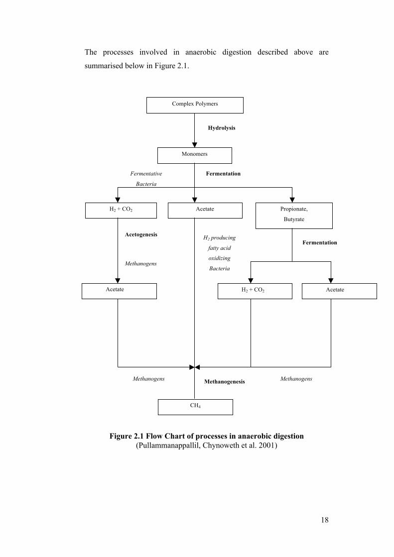
The processes involved in anaerobic digestion described above are

summarised below in Figure 2.1.

Figure 2.1 Flow Chart of processes in anaerobic digestion (Pullammanappallil, Chynoweth et al. 2001)

CH4

Methanogenesis

Acetate H2 + CO2 Acetate

Fermentation Acetogenesis

Complex Polymers

Monomers

H2 + CO2 Acetate Propionate,

Butyrate

Hydrolysis

Fermentation Fermentative

Bacteria

H2 producing

fatty acid

oxidizing

Bacteria Methanogens

Methanogens Methanogens

19

Complex organic compounds are hydrolysed to form simpler polymers

(monomers). The monomers are further broken down into volatile fatty

acids (acetate, propionate, butyrate) and H2 and CO2 by fermentative

bacteria. Methanogenic bacteria further break down the volatile fatty acids

to produce biogas.

Anaerobic digestion is commonly used for effluent and sewage treatment. In

developing countries, farm-based anaerobic digestion systems offer the

potential for cheap, low-cost energy for cooking and lighting facilities.

Anaerobic digestion techniques can help reduce the emission of greenhouse

gasses by replacement of fossil fuels. Improvement in anaerobic digestion

can be accomplished by multiple ways, some of which are optimisation of

the process conditions, pretreatment of input effluent and increase of

process temperature.

2.2 Mathematical Models in Anaerobic Digestion

Understanding and application of anaerobic treatment has made significant

progress in the past 30 years and numerous mathematical models have been

developed (Lyberatos and Skiadas 1999). The complexities of anaerobic

treatment and less experience with the process compared with its aerobic

counterpart are reasons for variations among models and lag in

standardisation of an anaerobic model. A review of previous models was

conducted to examine their applicability and inclusion of the significant

phenomena in anaerobic treatment. Some of the different approaches used

by researchers were:

• Models assuming substrate inhibited Monod kinetics of the

methanogens. e.g. (Graef and Andrews 1974; Hill and Barth 1977);

(Kleinstreuer and Powegha 1982); (Moletta, Verrier et al. 1986);

(Smith, Bordeaux et al. 1988)).

• Models where the influence of pH and volatile fatty acids is taken into

account. e.g. (Hill 1982); (Bryers 1985).

20

• Models where the process is primarily controlled by the hydrogen

concentration in the reactor. e.g. (Mosey 1983); (Pullammanappallil,

Owens et al. 1991); (Costello, Greenfield et al. 1991a); (Costello,

Greenfield et al. 1991b).

• Complex models assuming inhibition of compounds. e.g. (Angelidaki,

Ellegaard et al. 1993); (Siegrist, Renggli et al. 1993).

The first dynamic model for an anaerobic process was developed by

Andrews (Andrews 1969). A major limitation of this model was that the

pH was assumed to be constant. Graef and Andrews (1974) removed this

limitation by considering physico chemical interactions among the liquid,

gas and biological phases. They used the modified version of Monod

kinetics to consider the inhibition of methane formers by non ionised

VFA. It was assumed that the utilisation of acetic acid by methane formers

was rate limiting, as a result their model included only one group of

bacteria. The work of Graef and Andrews (Graef and Andrews 1974) was

considered by Hill and Barth (Hill and Barth 1977) to develop a model to

simulate anaerobic digestion of animal waste. A second bacterial

population was added to consider the VFA production by acid formers and

VFA utilization by methane formers. Particulate hydrolysis was also

incorporated into their model. They further modified the Monod

expression to include inhibition of methane formers by both ammonia and

nitrogen and VFA. Their model predicts general trends of anaerobic

digestion of animal manure.

An extensive model that considered the biological phase of anaerobic

digestion of glucose has been developed (Mosey 1983). Two important

advancements in the model were consideration of

• four populations of bacteria

• role of hydrogen gas in the formation of intermediate products of

acetic, propionic and butyric acids, and in the conversion of

intermediate products of propionate and butyrate into acetic acid.

21

Harper and Pohland (Harper and Pohland 1986) and (Mosey 1983)

indicated that hydrogen concentration in the digester controls the course of

substrate utilisation. Numerous studies on analysis of the thermodynamics

of reactions in anaerobic digestion have been conducted (McInerney and

Bryant 1981), (McInerney and Beaty 1988), (Harper and Pohland 1986)

and (Thauer and Jungermann 1977). The effect of hydrogen partial

pressure on the production of acetic acid, propionic and butyric acids was

determined.

Mosey (Mosey 1983) investigated the regulatory role of hydrogen by

considering the metabolic pathways of the acid forming bacteria. He

developed a comprehensive mathematical model for the utilisation of

glucose via the Embden-Meyerhof pathway, which converts glucose to

pyruvate. Mosey (Mosey 1983) related the relative availability of NAD+

and NADH to ρH2 to develop mathematical expressions that can predict the

relative production of acetic, propionic and butyric acids from the

utilization of glucose.

Mosey (Mosey 1983) also considered the reaction stoichiometries to

determine the regulation factor for each VFA produced from the

biodegradation of carbohydrates, as well as for the utilisation of butyric

and propionic acids.

The work of Mosey (Mosey 1983) was a keystone in the development of

more advanced models. A number of researchers, (Rozzi and Merlini

1985), (Jones 1989) and (Jones & Hall 1989) have developed models,

based on four population model of (Mosey 1983) for the biological phase

and the model of (Graef and Andrews 1974) for the physio chemical

system. These models predict change of individual VFA species, pH, pH2,

and biogas production and composition as a function of time. (Costello,

Greenfield et al. 1991a), (Costello, Greenfield et al. 1991b) developed a

six population model with a major change of introducing lactic acid

bacteria into the model of (Mosey 1983).

22

The mathematical models mentioned above and their respective process

flowcharts are further described in Appendix A.

2.3 Primary and Secondary Production

Aquaculture is an ancient practice for rearing aquatic organisms (Stickney

2000). Algae, zooplankton, molluscs and fish are grown in natural or

experimental designed basins. Phytodepuration is an important practice used

to recover clean water from wastewater for re-use and its characteristic is to

depress eutrophication and pollution (Brix and Scheirup 1989; Di Termini,

Prassone et al. 2011). In this process water to be purified is put in ponds

with specific phytoplankton and plants, which are efficient in uptake of

nutrients, therefore acting as biological filters. As a result they naturally

purify the water.

In the scientific literature a few papers connected with the study of

modelling integrated aquaculture dynamics can be found which could be

due to the aquaculture system’s complexity and the difficulty to adequately

describe them. There are three different approaches to modelling primary

and secondary production of species (Hamilton and Schladow 1997).

1. The most common modelling approach has been exemplified by the

development and application of steady state, input-output models.

Generally nutrient concentrations are calculated from net inputs and

chlorophyll-a concentration is predicted by correlation with the

limiting nutrient, most often phosphorus. Factors that can affect

phytoplankton biomass, such as light, climate, biological interactions

and internal loading of nutrients are not considered. The assumption

that the lake is a continuously mixed system is very restrictive and

only applicable at certain times of the year, if at all. The

shortcomings of such approaches include an inability to make

predictions in the face of varying physical and biological conditions,

and a failure to offer insights into the determinants of changing

water quality (Hamilton and Schladow 1997).

23

2. The second approach referred to as ecological water quality

modelling, specifically addresses many of the biological and

chemical factors that are absent in the simple input-output models.

Such models represent ecological processes by time varying,

interdependent conservation equations, with rate coefficients that

require calibration (Di Toro, O' Connor et al. 1971; Jørgensen,

Kamp-Nielsen et al. 1975; Jørgensen, Mejer et al. 1978; Scavia

1980; Matsuoka, Goda et al. 1986; Miyanaga 1986). The physical

processes of transport and mixing within the water body have

generally been oversimplified. Interactions between physical

processes and the biological and chemical processes described by

these models are poorly represented. The predictive abilities of these

models are compromised (Schladow and Hamilton 1997).

3. The third approach has been the extension of hydrodynamic models

to include water quality components, either by combination with

simple input-output models or more recently with ecological models.

The most common approach for the hydrodynamics has been to use

a one dimensional (1D) model, with retention of variables in the

vertical dimension. Process based hydrodynamic models have also

been identified and reported in literature (Stefan and Ford 1975;

Imberger, Patterson et al. 1978). These have been coupled with

ecological models giving the water quality models MINLAKE

(Riley and Stefan 1988) and CE-QUAL (USCE, 1986) respectively.

The models differ most in the extent to which the individual

processes are described (Schladow and Hamilton 1997).

Hydrodynamic and water quality models have become more abundant and

sophisticated since the early models which were developed in the 1970s

because of an increased demand for better models and an improvement in

the world of computing technology (Jørgensen, Jørgensen et al. 1981;

Jørgensen, Kamp-Nielsen et al. 1986; Jørgensen 1995).

The hydrodynamic models typically fall into one of the two categories; the

first are the relatively simple advective-diffusive models that require little

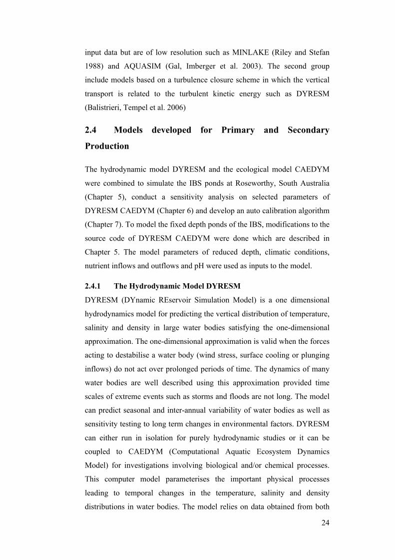
24

input data but are of low resolution such as MINLAKE (Riley and Stefan

1988) and AQUASIM (Gal, Imberger et al. 2003). The second group

include models based on a turbulence closure scheme in which the vertical

transport is related to the turbulent kinetic energy such as DYRESM

(Balistrieri, Tempel et al. 2006)

2.4 Models developed for Primary and Secondary

Production

The hydrodynamic model DYRESM and the ecological model CAEDYM

were combined to simulate the IBS ponds at Roseworthy, South Australia

(Chapter 5), conduct a sensitivity analysis on selected parameters of

DYRESM CAEDYM (Chapter 6) and develop an auto calibration algorithm

(Chapter 7). To model the fixed depth ponds of the IBS, modifications to the

source code of DYRESM CAEDYM were done which are described in

Chapter 5. The model parameters of reduced depth, climatic conditions,

nutrient inflows and outflows and pH were used as inputs to the model.

2.4.1 The Hydrodynamic Model DYRESM

DYRESM (DYnamic REservoir Simulation Model) is a one dimensional

hydrodynamics model for predicting the vertical distribution of temperature,

salinity and density in large water bodies satisfying the one-dimensional

approximation. The one-dimensional approximation is valid when the forces

acting to destabilise a water body (wind stress, surface cooling or plunging

inflows) do not act over prolonged periods of time. The dynamics of many

water bodies are well described using this approximation provided time

scales of extreme events such as storms and floods are not long. The model

can predict seasonal and inter-annual variability of water bodies as well as

sensitivity testing to long term changes in environmental factors. DYRESM

can either run in isolation for purely hydrodynamic studies or it can be

coupled to CAEDYM (Computational Aquatic Ecosystem Dynamics

Model) for investigations involving biological and/or chemical processes.

This computer model parameterises the important physical processes

leading to temporal changes in the temperature, salinity and density

distributions in water bodies. The model relies on data obtained from both

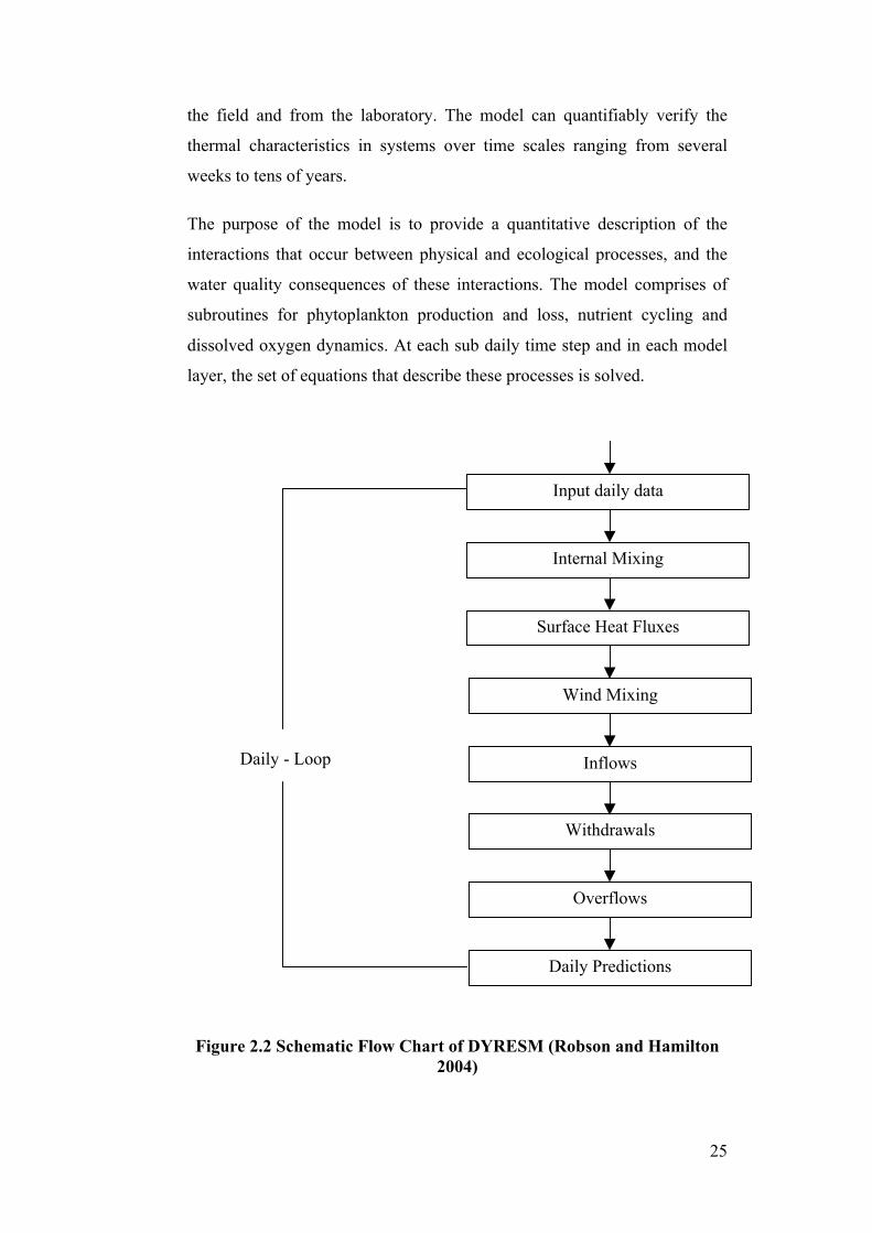
25

the field and from the laboratory. The model can quantifiably verify the

thermal characteristics in systems over time scales ranging from several

weeks to tens of years.

The purpose of the model is to provide a quantitative description of the

interactions that occur between physical and ecological processes, and the

water quality consequences of these interactions. The model comprises of

subroutines for phytoplankton production and loss, nutrient cycling and

dissolved oxygen dynamics. At each sub daily time step and in each model

layer, the set of equations that describe these processes is solved.

Daily - Loop

Figure 2.2 Schematic Flow Chart of DYRESM (Robson and Hamilton 2004)

Input daily data

Internal Mixing

Surface Heat Fluxes

Wind Mixing

Inflows

Withdrawals

Overflows

Daily Predictions

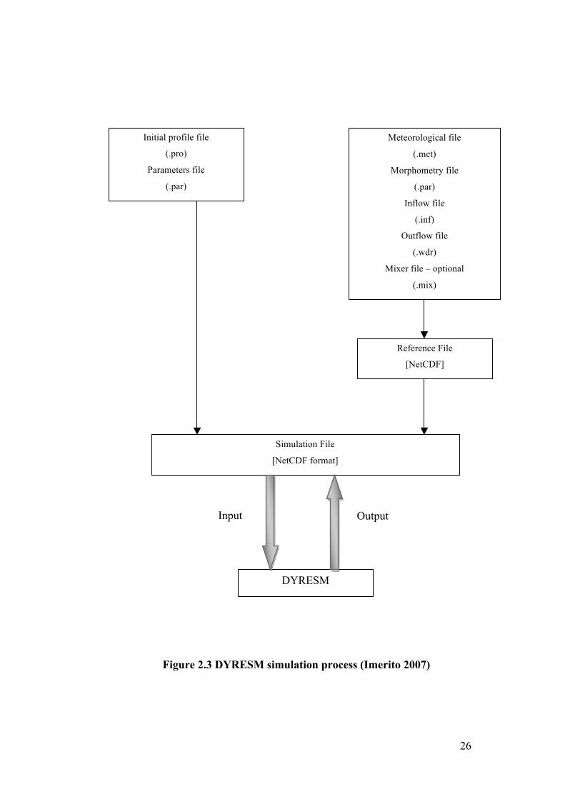
26

Figure 2.3 DYRESM simulation process (Imerito 2007)

Initial profile file

(.pro)

Parameters file

(.par)

Meteorological file

(.met)

Morphometry file

(.par)

Inflow file

(.inf)

Outflow file

(.wdr)

Mixer file – optional

(.mix)

Reference File

[NetCDF]

Simulation File

[NetCDF format]

DYRESM

Input Output

27

Flow chart of the DYRESM process is shown in Figure 2.2 and the

DYRESM simulation process is shown in Figure 2.3. The data from the

DYRESM input files e.g. meteorological, morphometry, inflow, outflow

and artificial mixing (optional) files is stored in a NetCDF reference file,

which along with the initial profile and parameters file forms a simulation

file in NetCDF format. This simulation file forms an input to the DYRESM

program.

DYRESM is based on a Lagrangian layer scheme and the layers are

adjusted to stay within user defined limits. The water body is modelled by a

series of horizontal layers of uniform property but variable thickness. The

layer positions change as inflow, outflow, evaporation and rainfall affect the

stored volume, and layer thicknesses change as the layers are moved

vertically to accommodate volume changes. An advantage of this layer

scheme is that it lends itself to the vertical structure of the water body. The

layers are counted from bottom to top.

Limits are set on the individual layer thicknesses and volumes. The upper

and lower limits are set to ensure that adequate resolution is achieved and

excessive number of layers is not used. To ensure that the layer structure is

stable, the individual layer densities are checked from top down. If the

upper layer density is higher than the layer immediately below, the two

layers are amalgamated and the layer properties conserved by appropriate

governing phenomenon. This process is repeated for all layers.

The density of water varies with the water temperature which causes

thermal stratification in the water body. When the temperature of the water

body decreases, the density usually decreases till the water temperature

reaches 4 0C. When salinity increases the density also increases. The density

of water (kg/m3) in a layer given its temperature (0C), salinity (psu),

pressure (bars) is given by the equation of state for density of salt water

(Imerito 2007).

28

( ) ( )

⎟⎟⎠

⎞⎜⎜⎝

⎛−

=

),,(1

0,,,,

PSTKPSTPST ρ

ρ Eq. 2.6

where ( ) 22/30,, DSCSBSAST +++=ρ Eq. 2.7

where A, B, C and D are polynomial functions of temperature.

To ensure stability of the layer structure, the individual layer densities are

calculated from top to bottom. If the upper layer density is higher than the

immediate layer below, the two layers are mixed and the layer properties are

conserved. This process is repeated for all layers culminating in a stable

structure.

The surface heat, mass and momentum exchange are the primary driving

mechanisms for DYRESM. The majority of the energy for heating, mixing

and stratifying the lake is obtained from these surface exchanges. The

surface exchanges include heating due to short wave radiation penetration

into the lake, and fluxes at the surface due to evaporation, sensible heat (i.e.

convection of heat from the water surface to the atmosphere), long wave

radiation and wind stress.

The density variations occurring in water bodies inhibits vertical motion

while horizontal density variations are minimised by lateral and longitudinal

convection, which occurs at a faster rate than vertical advection. DYRESM

provides a one-dimensional hydrodynamic platform for CAEDYM.

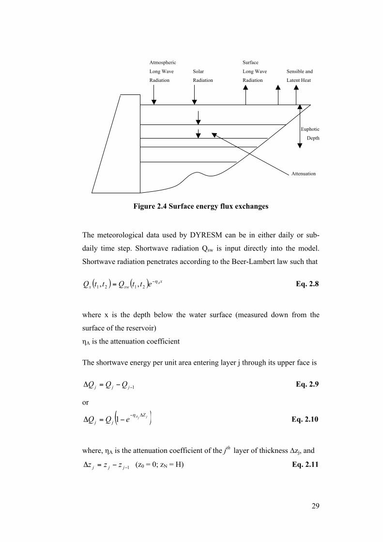
29

Atmospheric Surface

Long Wave Solar Long Wave Sensible and

Radiation Radiation Radiation Latent Heat

Euphotic

Depth

Attenuation

Figure 2.4 Surface energy flux exchanges

The meteorological data used by DYRESM can be in either daily or sub-

daily time step. Shortwave radiation Qsw is input directly into the model.

Shortwave radiation penetrates according to the Beer-Lambert law such that

( ) ( ) xswx

AettQttQ η−= 2121 ,, Eq. 2.8

where x is the depth below the water surface (measured down from the

surface of the reservoir)

ηA is the attenuation coefficient

The shortwave energy per unit area entering layer j through its upper face is

1−−=Δ jjj QQQ Eq. 2.9

or

( )jjA Zjj eQQ Δ−−=Δ

η1 Eq. 2.10

where, ηA is the attenuation coefficient of the jth layer of thickness ∆zj, and

1−−=Δ jjj zzz (z0 = 0; zN = H) Eq. 2.11

30

where, H is the depth of the water.

The penetrative short wave radiation has a wavelength of < 700 nm.

Radiation between 400-700 nm is defined as Photosynthetically Active

Radiation (PAR).

The net longwave radiation can be input into the model as incoming

longwave, net longwave or cloud cover data. The sensible heat loss from

the surface of the water body for the period ∆t can be calculated as (Imerito

2007)

( ) TTTUCCQ SaaPASS Δ−= ρ Eq. 2.12

where, CS is the sensible heat transfer coefficient for wind speed at 10 m

reference height above the water surface ( = 1.3 x 10-3)

ρA is the density of air in kg m-3

CP is the specific heat of air at constant pressure (= 1003 J kg-1K-1)

Ua is the wind speed at the standard reference height of 10 m in ms-1

Temperatures are either both in Celsius or both in Kelvin

The heat loss due to evaporation is given by (Imerito 2007)

( )[ ]⎭⎬⎫

⎩⎨⎧ Δ−= TTeeULC

PQ ssaaEALlh ρ

622.0,0min Eq. 2.13

where, P is the atmospheric pressure in hectopascals,

CL is the latent heat transfer coefficient (=1.3 x 10-3) for wind speed at a

reference height of 10 m,

ρA is the density of air in kg m-3,

LE is the latent heat of evaporation of water (=2.453 x 106 J kg-1),

Ua is the wind speed in ms-1 at a reference height of 10 m,

ea is the vapour pressure of air (hectopascals),

ea is the saturation vapour pressure at the water surface temperature TS

(hectopascals)

31

No condensation effects occurring in the numerical model, hence Qlh ≤ 0.

Thus, the total non penetrative energy density deposited in the surface layer

during the period ∆t is given by

lhswlwpennon QQQQ ++=− Eq. 2.14

The change in mass in the surface layer (layer number N) due to latent heat

flux is calculated as

( )v

NlhN L

AQlhM

−=Δ Eq. 2.15

where, AN is the surface area of the surface layer and LV is the latent heat of

vaporisation of water.

The change in surface layer mass due to rainfall is

( )d

hNNn NtRArainM Δ

=Δ ρ Eq. 2.16

where, Rh is the daily total rainfall in mm,

Nd is the number of seconds in a day

Therefore, the total mass change of the surface layer for the period ∆t is

( ) ( )rainMlhMM nnn Δ+Δ=Δ Eq. 2.17

The current model accounts for changes due to evaporation and

precipitation of pure water.

Surface Layer Mixing in DYRESM is undertaken with three specific

mechanisms: convective overturn, stirring and shear. The kinetic and

potential energies of the individual layers, starting at the surface layer, are

32

used to determine if the adjacent layers will mix. If there is sufficient energy

available, the layers will mix; any excess energy will be used to determine if

subsequent layers will mix. The amalgamation of layers ceases when there

is insufficient energy left, which is carried over to the next time step.

Turbulent Kinetic Energy (TKE) is introduced into the surface mixed layer

(SML) through the following processes:

Convective mixing: twAKE NNpconv Δ= −3*1ρη Eq. 2.18

Wind Stirring: tuAKE NNsstirr Δ= −3*1ρη Eq. 2.19

Shear Mixing: ( )211

1

2 −−

−

+= NN

NN

NNkshear UU

MMMM

KEη Eq. 2.20

where, ηp, ηs and ηk are efficiency coefficients,

ρN is the layer density,

Ai is the layer surface area,

Mi is the layer mass,

Ui is the layer speed,

∆t the model time – step

For water quality simulations using CAEDYM, bottom stress magnitudes

need to be calculated. This requires the epilimnion (top most layer in a

thermally stratified lake) and hypolimnion (dense, bottom layer of water in a

thermally stratified lake) water speeds to be determined, UE, and UH,

respectively. The epilimnion velocity, UE, is equal to the surface layer

velocity, UN, calculated as

( ) tzuU

NN Δ

Δ=

2*

Eq. 2.21

33

The velocity in the hypolimnion is calculated by

HEEHEH

EEH hhUhh

hhUU ≥<

⎩⎨⎧

= ;&; Eq. 2.22

where, hH and hE are the thicknesses of the hypolimnion and epilimnion

respectively.

Using the drag coefficient at the bottom, CD,bottom , the magnitudes of the

bottom stresses for the epilimnion and hypolimnion can be directly

calculated as

2, EEbottomDE UC ρτ = Eq. 2.23

2, HHbottomDH UC ρτ = Eq. 2.24

Inflows into DYRESM may be either surface (e.g. river or stream) or

subsurface (e.g. groundwater or pipe inflow) flows. The inflow to the water

body is modelled by inserting the volume into the layer of equal density,

taking into account the associated entrainment as the inflow passes through

the different layers. The layer structure is set within the limits set by the

user. Outflow occurs by the combination of withdrawals and overflow. The

required quantity of water is removed from the layer adjacent to the outlet.

If the amount of water exceeds the volume of the layer, then water is taken

from successive layers above the outlet until the required volume is

removed from the water column.

DYRESM can model two types of destratification systems-bubble plume

diffusers and surface mechanical mixers. Bubble plume diffusers consist of

a perforated pipe beneath the surface of water, through which compressed

air is pumped. As the air rises through the water column, it entrains fluid

and mixes the water column. DYRESM uses the simple buoyant plume

equations assuming that the plumes are circular and non-interacting.

34

The initial buoyancy flux is calculated as

71.0

⎟⎟⎠

⎞⎜⎜⎝

⎛=

diff

airairdiff PP

QQ Eq. 2.25

where, Qair is the free air flow rate of the compressor,

Pair is the air pressure (usually assumed as 101.3 kPa)

Pdiff is the pressure at the level of the diffuser due to both the atmosphere

and the depth of water,

Qdiff is the diffuser air flow rate.

The initial volumetric flow rate of entrained water is calculated as (Fisher,

List et al. 1979)

3/53/115

6 zBLbQ RPπ

α= Eq. 2.26

where, B is the buoyancy flux (m4s-3),

z is the bottom layer thickness (m),

b1 is a constant (= 4.7 (Fisher, List et al. 1979))

LR is the plume aspect ratio (assumed to be a constant of 0.1),

α is an entrainment coefficient (within the range 0.04-0.14).

The combined buoyancy flux of the air bubbles and entrained water is

calculated as

Pi

Piii QggQB ⎟⎟

⎠

⎞⎜⎜⎝

⎛ −−=

ρρρ

Eq. 2.27

where, ρi is the density of the current layer,

QP is the flow rate of the entrained volume.

The flow rate of the entrained volume in layer I is calculated as

( )1

3/51

3/53/115

6−

+−= − iPiiiRP QzzBLbQ πα Eq. 2.28

35

The development and process parameterisations of DYRESM have been

described extensively in literature (Imberger 1981; Hamilton, Schladow et

al. 1995; Hamilton and Schladow 1997; Schladow and Hamilton 1997;

Imerito 2007).

2.4.2 The Aquatic Ecological Model CAEDYM

CAEDYM (Hipsey, Romero et al. 2006) is an ecological model which

simulates the C, N, P, DO, and Si cycles along with inorganic suspended

solids, phytoplankton, and optional biotic compartments such as

zooplankton, fish, bacteria and others (Figure 2.5). CAEDYM can be linked

to hydrodynamic models like 1D DYRESM (Imerito 2007), DYRIM (a

quasi 2-D Lagrangian river floodplain model) and the 3D ELCOM (Hodges

and Dallimore 2001). The coupling between CAEDYM and the

hydrodynamic driver is dynamic.

Numerous optional biological and other state variables can also be

configured as per the requirements of the user. CAEDYM is more advanced

than traditional N-P-Z models as it can resolve species or group specific

ecological interactions. CAEDYM operates on any sub-daily time step and

is generally run at the same time interval as the hydrodynamic driver. The

user can specify if the same simulation is for freshwater, estuaries or coastal

water.

The major biogeochemical state variables in CAEDYM are given in Figure

2.5. The user can customize the input requirements by using a simple

configuration file. An input file for parameters can also be adjusted without

having to adjust the source code. However changes to the source code might

be required for specific variables of interest to the user.

Consequently CAEDYM was the most appropriate choice for simulating the

phytoplankton, zooplankton fish and nutrient dynamics in the aquaculture

section of the Integrated Biosystems. An extensive description of CAEDYM

can be found in (Hipsey, Romero et al. 2006).

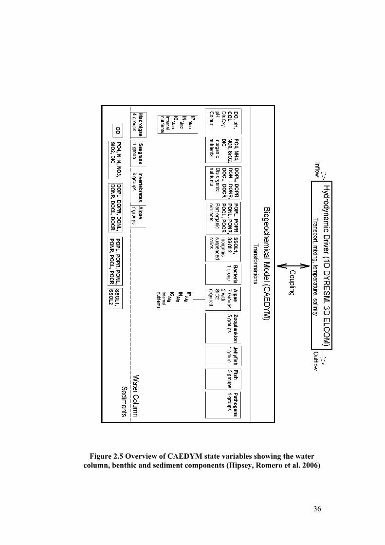
36

Figure 2.5 Overview of CAEDYM state variables showing the water column, benthic and sediment components (Hipsey, Romero et al. 2006)

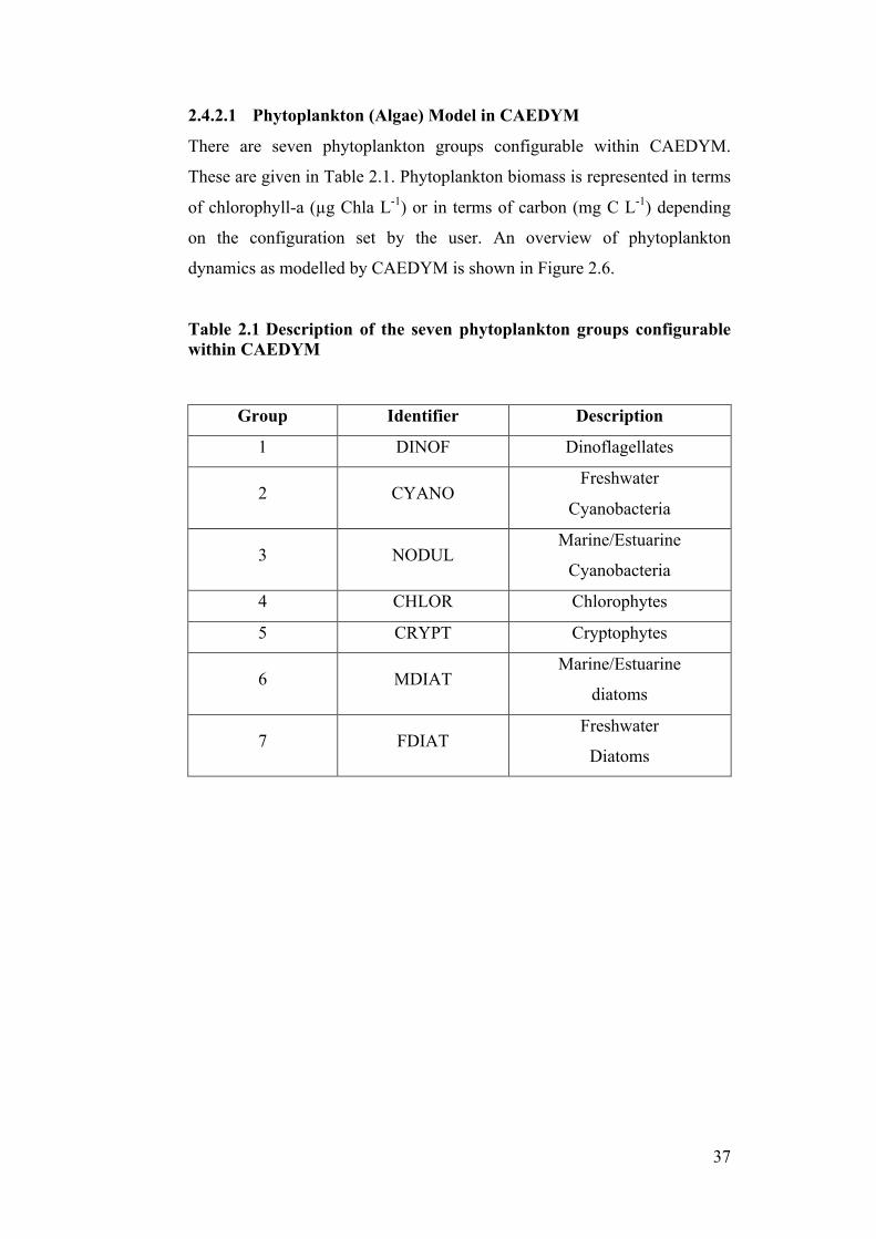
37

2.4.2.1 Phytoplankton (Algae) Model in CAEDYM

There are seven phytoplankton groups configurable within CAEDYM.

These are given in Table 2.1. Phytoplankton biomass is represented in terms

of chlorophyll-a (µg Chla L-1) or in terms of carbon (mg C L-1) depending

on the configuration set by the user. An overview of phytoplankton

dynamics as modelled by CAEDYM is shown in Figure 2.6.

Table 2.1 Description of the seven phytoplankton groups configurable within CAEDYM

Group Identifier Description

1 DINOF Dinoflagellates

2 CYANO Freshwater

Cyanobacteria

3 NODUL Marine/Estuarine

Cyanobacteria

4 CHLOR Chlorophytes

5 CRYPT Cryptophytes

6 MDIAT Marine/Estuarine

diatoms

7 FDIAT Freshwater

Diatoms

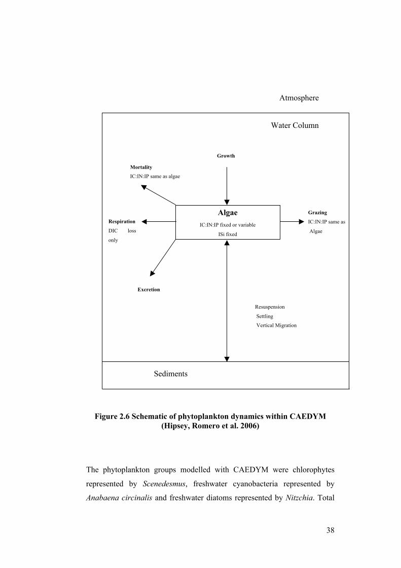
38

Figure 2.6 Schematic of phytoplankton dynamics within CAEDYM (Hipsey, Romero et al. 2006)

The phytoplankton groups modelled with CAEDYM were chlorophytes

represented by Scenedesmus, freshwater cyanobacteria represented by

Anabaena circinalis and freshwater diatoms represented by Nitzchia. Total

Respiration

DIC loss

only

Grazing

IC:IN:IP same as

Algae

Mortality

IC:IN:IP same as algae

Algae

IC:IN:IP fixed or variable

ISi fixed

Atmosphere

Water Column

Sediments

Growth

Resuspension

Settling

Vertical Migration

Excretion

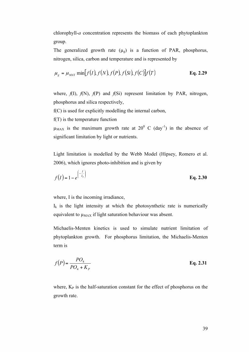
39

chlorophyll-a concentration represents the biomass of each phytoplankton

group.

The generalized growth rate (µg) is a function of PAR, phosphorus,

nitrogen, silica, carbon and temperature and is represented by

( ) ( ) ( ) ( ) ( )[ ] ( )TfCfSifPfNfIfMAXg ,,,,minµµ = Eq. 2.29

where, f(I), f(N), f(P) and f(Si) represent limitation by PAR, nitrogen,

phosphorus and silica respectively,

f(C) is used for explicitly modelling the internal carbon,

f(T) is the temperature function

µMAX is the maximum growth rate at 200 C (day-1) in the absence of

significant limitation by light or nutrients.

Light limitation is modelled by the Webb Model (Hipsey, Romero et al.

2006), which ignores photo-inhibition and is given by

( ) ⎟⎟⎠

⎞⎜⎜⎝

⎛−

−= kII

eIf 1 Eq. 2.30

where, I is the incoming irradiance,

Ik is the light intensity at which the photosynthetic rate is numerically

equivalent to µMAX if light saturation behaviour was absent.

Michaelis-Menten kinetics is used to simulate nutrient limitation of

phytoplankton growth. For phosphorus limitation, the Michaelis-Menten

term is

( )PKPO

POPf+

=4

4 Eq. 2.31

where, KP is the half-saturation constant for the effect of phosphorus on the

growth rate.

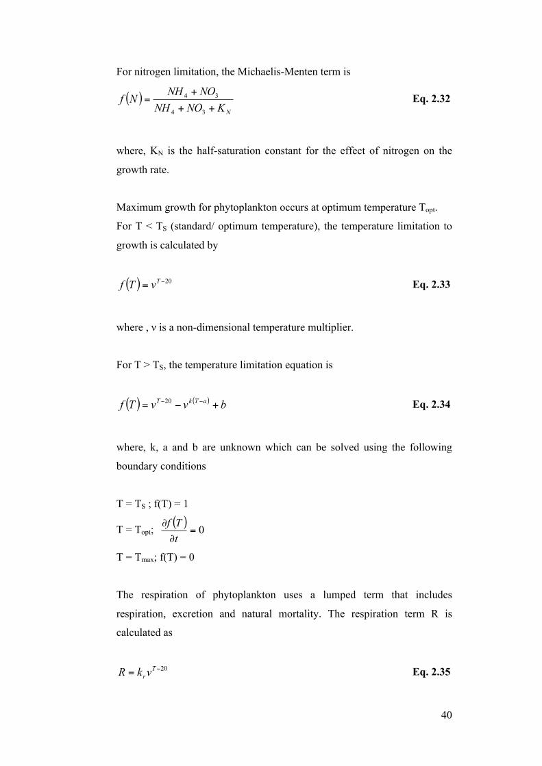
40

For nitrogen limitation, the Michaelis-Menten term is

( )NKNONH

NONHNf

++

+=

34

34 Eq. 2.32

where, KN is the half-saturation constant for the effect of nitrogen on the

growth rate.

Maximum growth for phytoplankton occurs at optimum temperature Topt.

For T < TS (standard/ optimum temperature), the temperature limitation to

growth is calculated by

( ) 20−= TvTf Eq. 2.33

where , ν is a non-dimensional temperature multiplier.

For T > TS, the temperature limitation equation is

( ) ( ) bvvTf aTkT +−= −−20 Eq. 2.34

where, k, a and b are unknown which can be solved using the following

boundary conditions

T = TS ; f(T) = 1

T = Topt; ( ) 0=∂

∂

tTf

T = Tmax; f(T) = 0

The respiration of phytoplankton uses a lumped term that includes

respiration, excretion and natural mortality. The respiration term R is

calculated as

20−= T

rvkR Eq. 2.35

41

where, kr is a respiration rate coefficient.

The environment described for the IBS is freshwater, so there is no

limitation by salinity. The respiration term can be adjusted to account for

grazing. Numerous improvements and changes to the source code were

required for CAEDYM to effectively model the aquaculture stages of the

IBS. These are discussed in detail in Chapter 5.

DYRESM accounts for dissolved oxygen dynamics in the water column

according to the following processes

• Air/ water surface exchange

• Phytoplankton photosynthesis and respiration

• Sediment chemistry

• Nitrification

Atmospheric exchange is based on the model of Wanninkhof (1992) given

by,

( )waterairOO CCkF −=22

Eq. 2.36

where, FO2 is the flux of oxygen across the air – water boundary (g m-2 s-1)

kO2 is the oxygen transfer coefficient (ms-1)

Cwater is the oxygen concentration in the surface waters near the interface

(gm-3)

Cair is the concentration of oxygen in the air phase near the interface (gm-3)

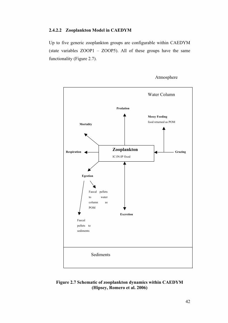
42

2.4.2.2 Zooplankton Model in CAEDYM

Up to five generic zooplankton groups are configurable within CAEDYM

(state variables ZOOP1 – ZOOP5). All of these groups have the same

functionality (Figure 2.7).

Figure 2.7 Schematic of zooplankton dynamics within CAEDYM (Hipsey, Romero et al. 2006)

Grazing

Faecal pellets

to water

column as

POM

Faecal

pellets to

sediments

Respiration

Excretion

Mortality

Egestion

Zooplankton IC:IN:IP fixed

Atmosphere

Water Column

Sediments

Messy Feeding

food returned as POM

Predation

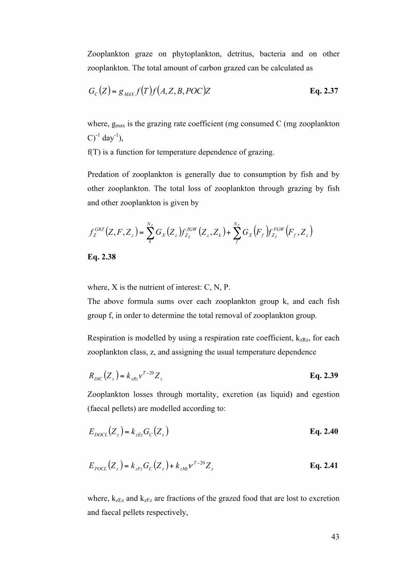
43

Zooplankton graze on phytoplankton, detritus, bacteria and on other

zooplankton. The total amount of carbon grazed can be calculated as

( ) ( ) ( )ZPOCBZAfTfgZG MAXC ,,,= Eq. 2.37

where, gmax is the grazing rate coefficient (mg consumed C (mg zooplankton

C)-1 day-1),

f(T) is a function for temperature dependence of grazing.

Predation of zooplankton is generally due to consumption by fish and by

other zooplankton. The total loss of zooplankton through grazing by fish

and other zooplankton is given by

( ) ( ) ( ) ( ) ( )zfFGWZ

N

ffXkz

ZGWZ

N

kzXz

GRZZ ZFfFGZZfZGZFZf

Z

F

Z

Z

,,,, ∑∑ +=

Eq. 2.38

where, X is the nutrient of interest: C, N, P.

The above formula sums over each zooplankton group k, and each fish

group f, in order to determine the total removal of zooplankton group.

Respiration is modelled by using a respiration rate coefficient, kzRz, for each

zooplankton class, z, and assigning the usual temperature dependence

( ) zT

zRzzDIC ZvkZR 20−= Eq. 2.39

Zooplankton losses through mortality, excretion (as liquid) and egestion

(faecal pellets) are modelled according to:

( ) ( )zCzEzzDOCL ZGkZE = Eq. 2.40

( ) ( ) zT

zMzzCzFzzPOCL ZkZGkZE 20−+= ν Eq. 2.41

where, kzEz and kzFz are fractions of the grazed food that are lost to excretion

and faecal pellets respectively,

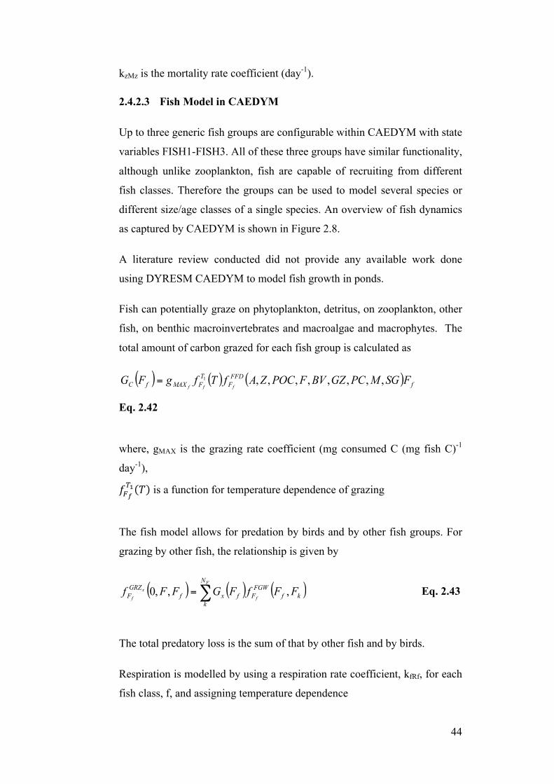
44

kzMz is the mortality rate coefficient (day-1).

2.4.2.3 Fish Model in CAEDYM

Up to three generic fish groups are configurable within CAEDYM with state

variables FISH1-FISH3. All of these three groups have similar functionality,

although unlike zooplankton, fish are capable of recruiting from different

fish classes. Therefore the groups can be used to model several species or

different size/age classes of a single species. An overview of fish dynamics

as captured by CAEDYM is shown in Figure 2.8.

A literature review conducted did not provide any available work done

using DYRESM CAEDYM to model fish growth in ponds.

Fish can potentially graze on phytoplankton, detritus, on zooplankton, other

fish, on benthic macroinvertebrates and macroalgae and macrophytes. The

total amount of carbon grazed for each fish group is calculated as

( ) ( ) ( ) fFFDF

TFMAXfC FSGMPCGZBVFPOCZAfTfgFG

fff,,,,,,,,1=

Eq. 2.42

where, gMAX is the grazing rate coefficient (mg consumed C (mg fish C)-1

day-1),

𝑓!!!! 𝑇 is a function for temperature dependence of grazing

The fish model allows for predation by birds and by other fish groups. For

grazing by other fish, the relationship is given by

( ) ( ) ( )kfFGWFf

N

kxf

GRZF FFfFGFFf

f

Fx

f,,,0 ∑= Eq. 2.43

The total predatory loss is the sum of that by other fish and by birds.

Respiration is modelled by using a respiration rate coefficient, kfRf, for each

fish class, f, and assigning temperature dependence

45

( ) fT

fRffDIC FkFR 20−= ν Eq. 2.44

Fish losses through mortality, excretion and egestion are modelled

according to

( ) ( )fCfEffDOCL FGkFE = Eq. 2.45

EDOCL Ff( ) = k fEfGC Ff( ) Eq. 2.46

( ) ( ) ( )[ ] ( ) fDOff

TfMffCfFffPOCL SfDOfFkFGkFE 120 1++= −ν Eq. 2.47

where, kfEf and kfFf are fractions of the grazed food that are lost to excretion

and faecal pellets respectively,

kfMf is the mortality rate coefficient (day-1).

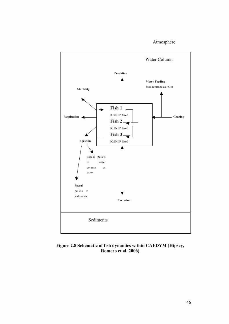
46

Figure 2.8 Schematic of fish dynamics within CAEDYM (Hipsey, Romero et al. 2006)

Grazing

Faecal pellets

to water

column as

POM

Faecal

pellets to

sediments

Respiration

Excretion

Mortality

Messy Feeding

food returned as POM

Predation

Egestion

Fish 1 IC:IN:IP fixed



Atmosphere

Water Column

Sediments

47

2.5 Techniques used in Water Quality Models Calibration

Mathematical model calibration is the process of determining the parameters

appearing in the equations of a model such that results produced by the

model agree closely with a set of measured data, in the context of the

selected objective function(s) (Ostfeld and Salomons 2005). The basic

approach in mathematical calibration is usually the same; an objective

function is designed to measure the agreement between measured (field)

data and the mathematical model simulated data for a particular set of

coefficients chosen by the user. The objective function ensures that small

values represent close agreement. The calibration process, which is a

constrained minimisation technique, adjusts the coefficient values within the

feasible domains to minimise the objective function.

It is an accepted fact that a mathematical model prediction should not be

deterministic, most probable representation, but should also explicitly

include an estimate of uncertainty. Mathematical models are characterised

by a certain degree of uncertainty, which results from both uncertainties in

modelled processes and observation errors, and the structural and numerical

errors of the mathematical model. Good modelling practice requires the

modeller to provide an evaluation of the confidence of the model predictions

(Ratto, Tarantola et al. 2001). This enables the researcher to assess the

uncertainties associated with the outcome (response) of the model itself.

Uncertainty Analysis (UA) and Sensitivity Analysis (SA) are pre requisites

for model building in any field where models are used. Model uncertainty

can be accounted for by the application of parametric uncertainty

methodologies and conditioning model predictions on observations.

Realistic assessment of these various sources of uncertainty is important for

science based decision making and will help direct resources towards model

structural improvements and uncertainty reduction (Blasone, Vrugt et al.

2008).

There has been an increase in number of methods in recent years to derive

meaningful uncertainty bounds on model predictions. Some of the methods

to represent model parameter, state and prediction uncertainty include

48

classical Bayesian (Kuczera and Parent 1998; Thiemann, Trosset et al.

2001; Vrugt, Gupta et al. 2003), pseudo-Bayesian (Beven and Binley 1992;

Freer, Beven et al. 1996), set-theoretic (Klepper, Scholten et al. 1991),

multiple criteria (Gupta, Sorooshian et al. 1998; Yapo, Gupta et al. 1998;

Boyle, Gupta et al. 2000; Madsen 2000; Madsen 2003; Vrugt, Gupta et al.

2003), sequential data assimilation (Moradkhani, Hsu et al. 2005; Vrugt,

Diks et al. 2005) and multi model averaging methods (Georgakakos, Seo et

al. 2004; Vrugt and Robinson 2007). These methods differ in their

assumptions and how the different sources of error are being treated.

Proper calibration and validation of a model require huge amounts of data

representing the various variables of interest. This involves a large number

of model parameters. Therefore, rigorous parameterisation and reduction of

the parameter space are essential to facilitate the calibration process and

make it more robust. Over parameterisation must be avoided to ensure a

higher degree of credibility to the model prediction (Andersen, Refsgaard et

al. 2001).

Refsgaard (1997) suggested assessing the parameter values from field data

as much as possible and fixing spatial patterns of parameters to simplify the

calibration process. Refsgaard (Refsgaard 1997) also suggested reduction in

the dimensionality of the parameter space by means of a sensitivity analysis

on the model output(s). By conducting a sensitivity analysis, the parameters

that do not influence the model response can be identified and fixed to their

prior values (Christiaens and Feyen 2001; Mertens, Madsen et al. 2004;

Muleta and Nicklow 2005). Sonnenborg used a method to decrease the

number of calibration parameters by fixing some of the pre-estimated

parameters by using a simpler model. He used the calibration results found

under steady state conditions to constrain the parameter space of a transient

model (Henriksen, Troldborg et al. 2003; Sonnenborg, Christensen et al.

2003). Refsgaard (1997) also pointed out that not only time validation but

also a multi site validation should be performed. If the model is used with

different discretisation scales, the dependency of the processes on the

different modelling scales should also be tested (Vázquez and Feyen 2007).

49

Data requirements can be an obstacle for a proper model validation because

spatially distributed time series observations of all the variables are rarely

available. This is one of the main reasons for distributed models being

calibrated and validated against discharge data (Andersen, Refsgaard et al.

2001; Engeland, Braud et al. 2006; McMichael, Hope et al. 2006). Madsen

proposed a framework for use of multiple criteria to measure the model

performance, which is crucial in calibration and validation of distributed

models. His method allowed modellers to include the different variables of

interest (multi-variable criteria), their spatial variability (multi-site criteria)

and the different error functions applied for evaluating the performance of

the simulated variables (multi-response criteria) (Madsen 2003). Inspite of

this, there hasn’t been much work done on integrating/ incorporating the

different methods together. Few studies have used multi-variable and multi-

site data to calibrate and validate an integrated, distributed model

(Refsgaard 1997; Madsen 2003; Vázquez and Feyen 2007). The last

component of this project aims at addressing this gap in research by

developing an auto calibration script for DYRESM CAEDYM which is a

multi-variable model presented in Chapter 7.

There are various difficulties in comparing uncertainty analysis techniques

in mathematical modelling of water bodies. Most techniques are different in

their philosophies with respect to parameter distribution, likelihood function

and /or objective function. Different concepts on objective functions lead to

different results depending on whether to maximise or minimise the

objective function. Due to the complexity of mathematical models running

hydrological processes, a higher number of model runs are needed to

calibrate and assess the uncertainty, due to the larger dimensionality of the

parameter space. There is a need to apply more efficient calibration and

uncertainty assessment procedures to minimise the computational burden.

2.5.1 GLUE

The Generalized Likelihood Uncertainty Estimation (GLUE) method

inspired by (Hornberger and Spear 1981) is a method for investigating the

uncertainties in the water resources and environmental modelling (Beven

50

and Binley 1992; Beven 1993). It has been widely studied by researchers

and applied in determining hydrological modelling uncertainty (Vogel,

Batchelder et al. ; Freer, Beven et al. 1996; Aronica, Hankin et al. 1998;

Cameron, Beven et al. 1999; Aronica, Bates et al. 2002; Freer, McMillan et

al. 2004; Montanari 2005; Heidari, Saghafian et al. 2006; Mantovan and

Todini 2006; McMichael, Hope et al. 2006). This method maps the

uncertainty in the modelling process onto the parameter space and operates

within the context of Monte Carlo (MC) analysis coupled with Bayesian

estimation and propagation of uncertainty. The GLUE technique calls for

rejecting the concept of a unique global optimum parameter set within some

particular model structure; instead it recognizes the acceptability within a

model structure of different parameter sets that are similarly good in

producing fit model predictions (Blasone, Vrugt et al. 2008). This concept is

defined as equifinality and is directly addressed by the computation of

different sets of parameters within a pseudo-Bayesian Monte Carlo

framework. The outputs of GLUE procedure are parameter distributions

within the limits of available observational data and associated uncertainty

bounds.

The GLUE methodology has been applied for uncertainty assessment in

environment modelling, including rainfall-runoff modelling (Beven and

Binley 1992; Freer, Beven et al. 1996; Lamb, Beven et al. 1998),

groundwater modelling (Feyen, Beven et al. 2001), unsaturated zone

modelling (Mertens, Madsen et al. 2004), flood inundation modelling

(Pappenberger, Beven et al. 2005; Pappenberger, Beven et al. 2007) and

distributed hydrological modelling (Mertens, Madsen et al. 2004;

McMichael, Hope et al. 2006; Choi and Beven 2007). The reason for GLUE

technique being implemented in different modelling scenarios is explained

by its conceptual simplicity, relative ease of implementation and use, and its

ability to handle different error structures and models without major

modifications to the method itself.

The GLUE procedure is based upon making a large number of runs of a

given model with different sets of factor values chosen randomly. The

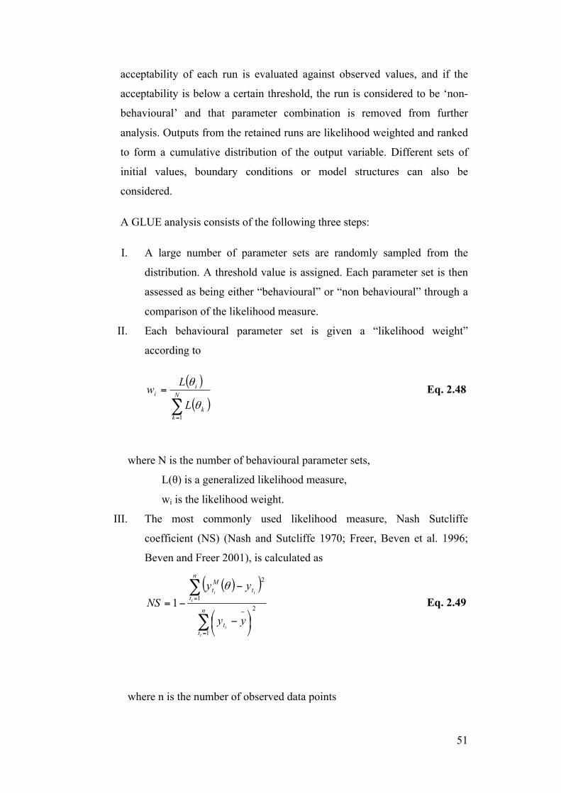
51

acceptability of each run is evaluated against observed values, and if the

acceptability is below a certain threshold, the run is considered to be ‘non-

behavioural’ and that parameter combination is removed from further

analysis. Outputs from the retained runs are likelihood weighted and ranked

to form a cumulative distribution of the output variable. Different sets of

initial values, boundary conditions or model structures can also be

considered.

A GLUE analysis consists of the following three steps:

I. A large number of parameter sets are randomly sampled from the

distribution. A threshold value is assigned. Each parameter set is then

assessed as being either “behavioural” or “non behavioural” through a

comparison of the likelihood measure.

II. Each behavioural parameter set is given a “likelihood weight”

according to

( )

( )∑=

= N

kk

ii

L

Lw

1

θ

θ Eq. 2.48

where N is the number of behavioural parameter sets,

L(θ) is a generalized likelihood measure,

wi is the likelihood weight.

III. The most commonly used likelihood measure, Nash Sutcliffe

coefficient (NS) (Nash and Sutcliffe 1970; Freer, Beven et al. 1996;

Beven and Freer 2001), is calculated as

( )( )

∑

∑

=

−

=

⎟⎠⎞

⎜⎝⎛ −

−

−=n

tt

n

tt

Mt

t

i

i

ii

yy

yyNS

1

21

2

1θ

Eq. 2.49

where n is the number of observed data points

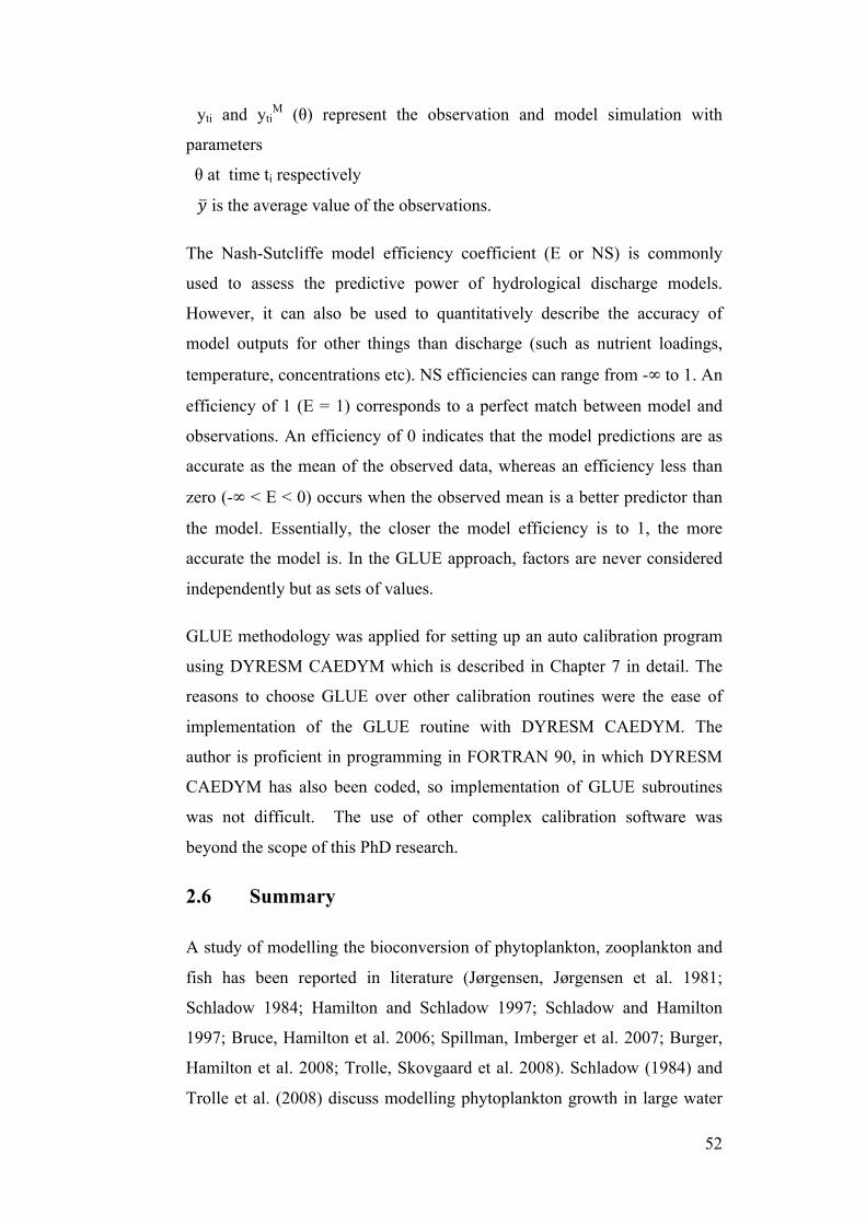
52

yti and ytiM (θ) represent the observation and model simulation with

parameters

θ at time ti respectively

𝑦 is the average value of the observations.

The Nash-Sutcliffe model efficiency coefficient (E or NS) is commonly

used to assess the predictive power of hydrological discharge models.

However, it can also be used to quantitatively describe the accuracy of

model outputs for other things than discharge (such as nutrient loadings,

temperature, concentrations etc). NS efficiencies can range from -∞ to 1. An

efficiency of 1 (E = 1) corresponds to a perfect match between model and

observations. An efficiency of 0 indicates that the model predictions are as

accurate as the mean of the observed data, whereas an efficiency less than

zero (-∞ < E < 0) occurs when the observed mean is a better predictor than

the model. Essentially, the closer the model efficiency is to 1, the more

accurate the model is. In the GLUE approach, factors are never considered

independently but as sets of values.

GLUE methodology was applied for setting up an auto calibration program

using DYRESM CAEDYM which is described in Chapter 7 in detail. The

reasons to choose GLUE over other calibration routines were the ease of

implementation of the GLUE routine with DYRESM CAEDYM. The

author is proficient in programming in FORTRAN 90, in which DYRESM

CAEDYM has also been coded, so implementation of GLUE subroutines

was not difficult. The use of other complex calibration software was

beyond the scope of this PhD research.

2.6 Summary

A study of modelling the bioconversion of phytoplankton, zooplankton and

fish has been reported in literature (Jørgensen, Jørgensen et al. 1981;

Schladow 1984; Hamilton and Schladow 1997; Schladow and Hamilton

1997; Bruce, Hamilton et al. 2006; Spillman, Imberger et al. 2007; Burger,

Hamilton et al. 2008; Trolle, Skovgaard et al. 2008). Schladow (1984) and

Trolle et al. (2008) discuss modelling phytoplankton growth in large water

53

bodies, while Bruce et al. (2006) discloses modelling of zooplankton growth

and nutrient dynamics in lakes. There is minimal literature available for

modelling fish using DYRESM CAEDYM. These models have been

developed in individual water bodies but not as part of an IBS where the

output of effluent from the algal pond forms an input to the zooplankton

pond and an output of effluent from the zooplankton pond forms an input to

the fish pond. The aquaculture model DYRESM CAEDYM has been

applied extensively to ponds of large depth to model phytoplankton,

zooplankton and fish (Schladow and Hamilton 1997; Trolle, Skovgaard et

al. 2008). Application of the DYRESM CAEDYM model to ponds of

shallow depth (~1 m) has not been reported in literature. Modelling of the

IBS ponds of 1m depth reported in this thesis will help close the gap in the

literature.

There is minimal literature available relating use of an auto calibration

routine to calibrate the parameters used in CAEDYM. The conventional

process of “trial and error” of calibrating parameters is tedious and

inefficient. More investigation is required to incorporate an automatic

calibration program into DYRESM CAEDYM to provide an efficient and

effective method of model parameter calibration and validation. This PhD

research will enable the use of a software routine to automatically calibrate

the parameters used in CAEDYM when the simulated data is modelled

against real time data.

54

3 Experimental Methods and Data

Collection

3.1 Introduction

The aim of this PhD research is to develop a mathematical model for a

commercial scale IBS and to test the suitability of DYRESM CAEDYM as

a control and management tool for the IBS. In order to achieve this,

microcosm experiments were conducted to develop further research into the

IBS. A pilot plant anaerobic digestion system and an aquaculture mesocosm

facility were developed which replicated the functioning of an IBS at a

laboratory level. After completing successful trials of the mesocosm facility,

a design of the commercial scale IBS was developed with additional

facilities for research and development. The commercial scale IBS however

could not be constructed at the time this research was conducted due to

certain administrative and financial restrictions which were beyond the

control of the researcher. Therefore experimental data collected from both

the pilot plant and the mesocosm facility (pilot IBS) were used for

developing a model and assessing its suitability for the commercial scale

IBS.

In this Chapter, Stage 1 experiments used for data collection and anaerobic

digestion are reported. The anaerobic digestion experiments were

undertaken to provide data which were the inputs for the development of the

aquaculture model (described in Chapter 5). Approximately 18 months

(from February 2005 – September 2006) were required for the set up and

installation of the two stage anaerobic digestion system and the Integrated

Aquaculture System. These systems were the backbone of the research work

to be discussed in later chapters.

This chapter is organised as follows.

• Section 3.2 describes the set up, installation and commissioning of

the pilot scale two stage anaerobic digestion system.

55

• Section 3.5 discusses the set up and installation of the pilot scale

Integrated Aquaculture system (mesocosm facility) for the

aquaculture stages of the IBS.

• Sections 3.6 and 3.7 describe the experiments conducted for the

bioconversion of algae.

• Finally section 3.8 describes the batch scale anaerobic digestion

experiments which generated data for input into the aquaculture

model.

3.2 Set up of the Pilot Scale Two-Stage Anaerobic

Digestion System

3.2.1 Equipment: Reactors and Digesters

A pilot scale two-stage anaerobic digestion system was set up in the

Breakwell laboratory at the Roseworthy Campus, The University of

Adelaide, South Australia. Active involvement in the construction and set

up of the anaerobic digestion system with the post doctoral researchers was

important as it provided an opportunity to understand the anaerobic

digestion stage of the IBS process. The main objectives of this pilot scale

system were to conduct experiments to maximise throughput of raw piggery

effluent, whilst maintaining high biogas generation.

Parameters measured from the experiments conducted were

• Chemical Oxygen Demand (COD)

• Soluble COD (SCOD)

• Total COD (TCOD)

• Total Kjeldahl Nitrogen (TKN) and Total Ammonia Nitrogen (TAN)

• Total and Soluble Phosphorus (TP, SP)

• Volatile Fatty Acids (VFA)

• Total and Volatile Solids (TS, VS)

• Organic Loading Rate (OLR)

• Biogas composition

56

• Biogas volume

• Temperature

• pH

These parameters were necessary to record as they formed an input to the

anaerobic digestion and aquaculture models. COD, TAN, TP, SP and biogas

volume were used for the development of the anaerobic digestion model

while TAN, SP and pH formed inputs and outputs from the aquaculture

model DYRESM CAEDYM.

The two-stage anaerobic digestion system which comprised a thermophilic

and mesophilic digesters is shown in Figure 3.2 and Figure 3.3.

Thermophilic Digesters: Two 200 L stainless steel tanks were used as

thermophilic digesters for the experiments. A microprocessor based

controller was used to ensure a constant operational temperature in the

reactors. A centrifugal pump was connected to the reactors to enable

pumping of piggery effluent and hourly recirculation of acidifying effluent

within the reactors. In addition, hourly temperatures and gas production in

the reactors were continuously monitored and recorded by a data logger

interfaced with a computer.

Mesophilic Digesters: Four 225 L plug flow type digesters (polydigesters)

were used to further digest the effluent under ambient conditions. These

digesters had an inlet and outlet located at each end for conveying the

influent and effluent respectively. The hourly temperatures and gas

production in the digesters were monitored and recorded hourly using a data

logger.

pH was measured in both digesters using a pH measuring device (Thermo

Scientific, Eutech Instruments, PC 650). Temperature was measured using

RTD thermocouples (Temperature Controls Pty. Ltd.). Gas production in

the digesters was recorded using positive displacement type gas meters

comprising a float switch and solenoid valve.

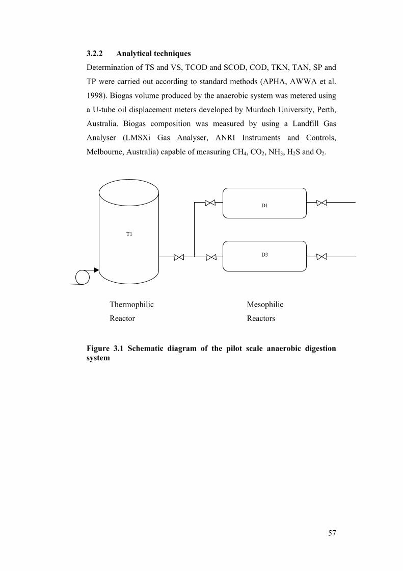
57

3.2.2 Analytical techniques

Determination of TS and VS, TCOD and SCOD, COD, TKN, TAN, SP and

TP were carried out according to standard methods (APHA, AWWA et al.

1998). Biogas volume produced by the anaerobic system was metered using

a U-tube oil displacement meters developed by Murdoch University, Perth,

Australia. Biogas composition was measured by using a Landfill Gas

Analyser (LMSXi Gas Analyser, ANRI Instruments and Controls,

Melbourne, Australia) capable of measuring CH4, CO2, NH3, H2S and O2.

Figure 3.1 Schematic diagram of the pilot scale anaerobic digestion system

T1

D1

D3

Thermophilic

Reactor

Mesophilic

Reactors

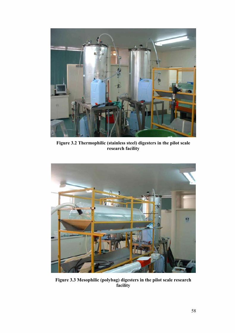
58

Figure 3.2 Thermophilic (stainless steel) digesters in the pilot scale

research facility

Figure 3.3 Mesophilic (polybag) digesters in the pilot scale research facility

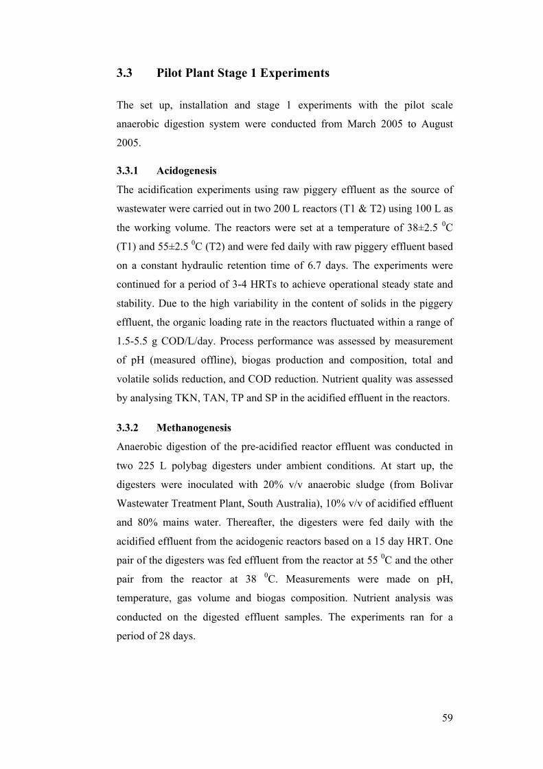
59

3.3 Pilot Plant Stage 1 Experiments

The set up, installation and stage 1 experiments with the pilot scale

anaerobic digestion system were conducted from March 2005 to August

2005.

3.3.1 Acidogenesis

The acidification experiments using raw piggery effluent as the source of

wastewater were carried out in two 200 L reactors (T1 & T2) using 100 L as

the working volume. The reactors were set at a temperature of 38±2.5 0C

(T1) and 55±2.5 0C (T2) and were fed daily with raw piggery effluent based

on a constant hydraulic retention time of 6.7 days. The experiments were

continued for a period of 3-4 HRTs to achieve operational steady state and

stability. Due to the high variability in the content of solids in the piggery

effluent, the organic loading rate in the reactors fluctuated within a range of

1.5-5.5 g COD/L/day. Process performance was assessed by measurement

of pH (measured offline), biogas production and composition, total and

volatile solids reduction, and COD reduction. Nutrient quality was assessed

by analysing TKN, TAN, TP and SP in the acidified effluent in the reactors.

3.3.2 Methanogenesis

Anaerobic digestion of the pre-acidified reactor effluent was conducted in

two 225 L polybag digesters under ambient conditions. At start up, the

digesters were inoculated with 20% v/v anaerobic sludge (from Bolivar

Wastewater Treatment Plant, South Australia), 10% v/v of acidified effluent

and 80% mains water. Thereafter, the digesters were fed daily with the

acidified effluent from the acidogenic reactors based on a 15 day HRT. One

pair of the digesters was fed effluent from the reactor at 55 0C and the other

pair from the reactor at 38 0C. Measurements were made on pH,

temperature, gas volume and biogas composition. Nutrient analysis was

conducted on the digested effluent samples. The experiments ran for a

period of 28 days.

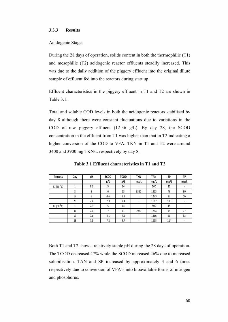
60

3.3.3 Results

Acidogenic Stage:

During the 28 days of operation, solids content in both the thermophilic (T1)

and mesophilic (T2) acidogenic reactor effluents steadily increased. This

was due to the daily addition of the piggery effluent into the original dilute

sample of effluent fed into the reactors during start up.

Effluent characteristics in the piggery effluent in T1 and T2 are shown in

Table 3.1.

Total and soluble COD levels in both the acidogenic reactors stabilised by

day 8 although there were constant fluctuations due to variations in the

COD of raw piggery effluent (12-36 g/L). By day 28, the SCOD

concentration in the effluent from T1 was higher than that in T2 indicating a

higher conversion of the COD to VFA. TKN in T1 and T2 were around

3400 and 3900 mg TKN/L respectively by day 8.

Table 3.1 Effluent characteristics in T1 and T2

Both T1 and T2 show a relatively stable pH during the 28 days of operation.

The TCOD decreased 47% while the SCOD increased 46% due to increased

solubilisation. TAN and SP increased by approximately 3 and 6 times

respectively due to conversion of VFA’s into bioavailable forms of nitrogen

and phosphorus.

Process Day pH SCOD TCOD TKN TAN SP TPg/L g/L mg/L mg/L mg/L mg/L

T1#(55#0C) 1 8.1 5 14 #, 500 15 #,8 8 6 13 3360 1223 46 8017 8 4.6 8.8 #, 1273 27 5628 7.4 7.3 7.4 #, 1667 100 #,

T2#(38#0C) 1 7.9 5 14 #, 500 15 #,8 7.6 7 11 3920 1284 49 7717 7.6 4.1 7.6 #, 1466 50 5328 7.3 7.2 9.7 #, 1658 114 ,#

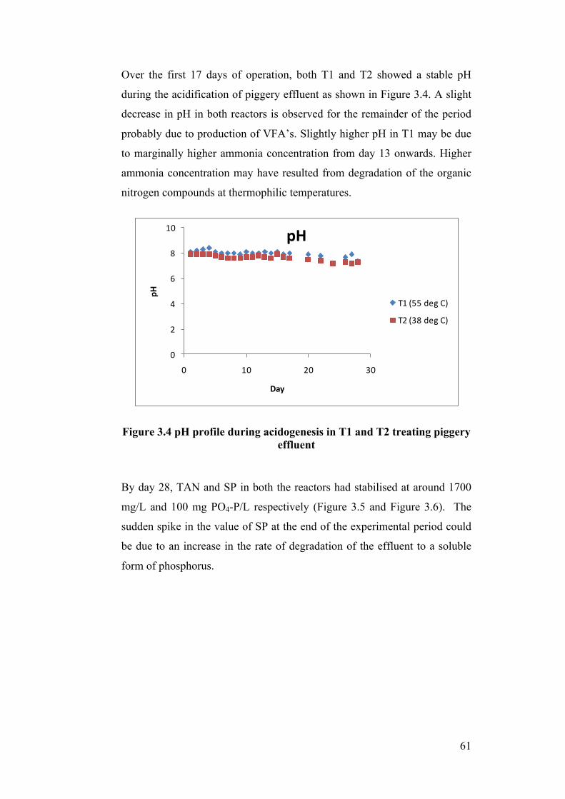
61

Over the first 17 days of operation, both T1 and T2 showed a stable pH

during the acidification of piggery effluent as shown in Figure 3.4. A slight

decrease in pH in both reactors is observed for the remainder of the period

probably due to production of VFA’s. Slightly higher pH in T1 may be due

to marginally higher ammonia concentration from day 13 onwards. Higher

ammonia concentration may have resulted from degradation of the organic

nitrogen compounds at thermophilic temperatures.

Figure 3.4 pH profile during acidogenesis in T1 and T2 treating piggery effluent

By day 28, TAN and SP in both the reactors had stabilised at around 1700

mg/L and 100 mg PO4-P/L respectively (Figure 3.5 and Figure 3.6). The

sudden spike in the value of SP at the end of the experimental period could

be due to an increase in the rate of degradation of the effluent to a soluble

form of phosphorus.

0

2

4

6

8

10

0 10 20 30

pH

Day

pH

T1 (55 deg C)

T2 (38 deg C)

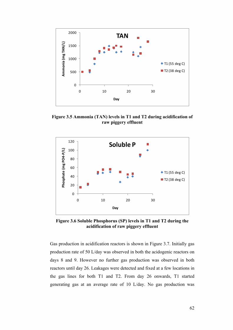
62

Figure 3.5 Ammonia (TAN) levels in T1 and T2 during acidification of raw piggery effluent

Figure 3.6 Soluble Phosphorus (SP) levels in T1 and T2 during the

acidification of raw piggery effluent

Gas production in acidification reactors is shown in Figure 3.7. Initially gas

production rate of 50 L/day was observed in both the acidogenic reactors on

days 8 and 9. However no further gas production was observed in both

reactors until day 26. Leakages were detected and fixed at a few locations in

the gas lines for both T1 and T2. From day 26 onwards, T1 started

generating gas at an average rate of 10 L/day. No gas production was

0

500

1000

1500

2000

0 10 20 30

Ammon

ia (m

g TA

N/L)

Day

TAN

T1 (55 deg C)

T2 (38 deg C)

0

20

40

60

80

100

120

0 10 20 30

Phosph

ate (m

g PO

4-‐P/L)

Day

Soluble P

T1 (55 deg C)

T2 (38 deg C)

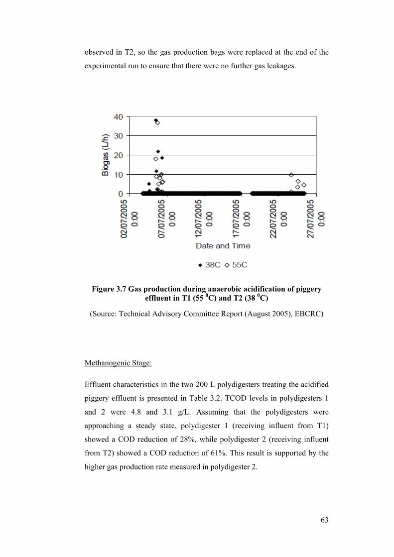
63

observed in T2, so the gas production bags were replaced at the end of the

experimental run to ensure that there were no further gas leakages.

Figure 3.7 Gas production during anaerobic acidification of piggery effluent in T1 (55 0C) and T2 (38 0C)

(Source: Technical Advisory Committee Report (August 2005), EBCRC)

Methanogenic Stage:

Effluent characteristics in the two 200 L polydigesters treating the acidified

piggery effluent is presented in Table 3.2. TCOD levels in polydigesters 1

and 2 were 4.8 and 3.1 g/L. Assuming that the polydigesters were

approaching a steady state, polydigester 1 (receiving influent from T1)

showed a COD reduction of 28%, while polydigester 2 (receiving influent

from T2) showed a COD reduction of 61%. This result is supported by the

higher gas production rate measured in polydigester 2.

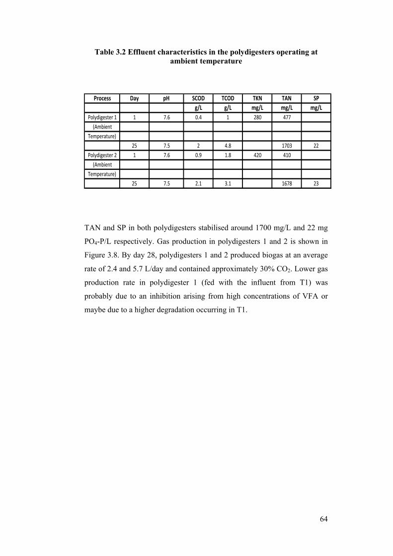
64

Table 3.2 Effluent characteristics in the polydigesters operating at ambient temperature

TAN and SP in both polydigesters stabilised around 1700 mg/L and 22 mg

PO4-P/L respectively. Gas production in polydigesters 1 and 2 is shown in

Figure 3.8. By day 28, polydigesters 1 and 2 produced biogas at an average

rate of 2.4 and 5.7 L/day and contained approximately 30% CO2. Lower gas

production rate in polydigester 1 (fed with the influent from T1) was

probably due to an inhibition arising from high concentrations of VFA or

maybe due to a higher degradation occurring in T1.

Process Day pH SCOD TCOD TKN TAN SPg/L g/L mg/L mg/L mg/L

Polydigester,1 1 7.6 0.4 1 280 477(Ambient

Temperature)25 7.5 2 4.8 1703 22

Polydigester,2 1 7.6 0.9 1.8 420 410(Ambient

Temperature)25 7.5 2.1 3.1 1678 23

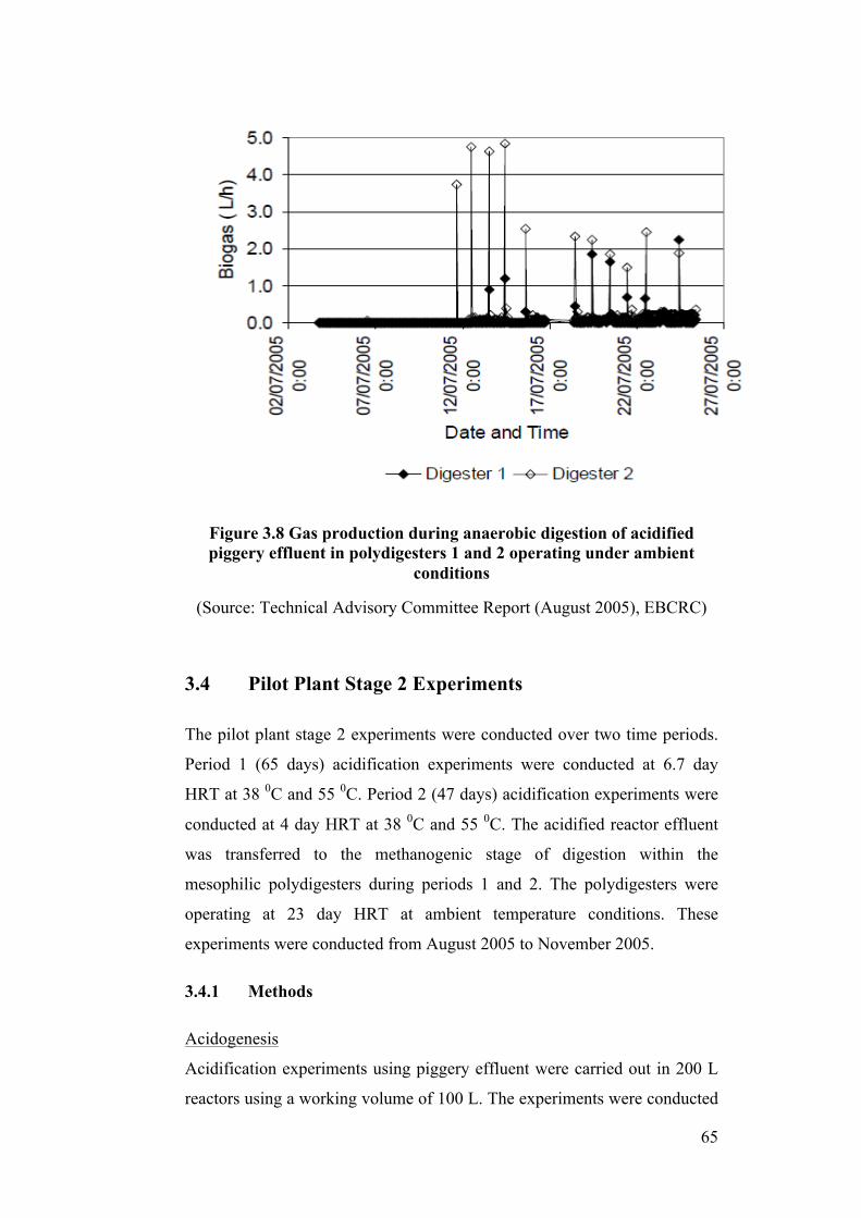
65

Figure 3.8 Gas production during anaerobic digestion of acidified piggery effluent in polydigesters 1 and 2 operating under ambient

conditions

(Source: Technical Advisory Committee Report (August 2005), EBCRC)

3.4 Pilot Plant Stage 2 Experiments

The pilot plant stage 2 experiments were conducted over two time periods.

Period 1 (65 days) acidification experiments were conducted at 6.7 day

HRT at 38 0C and 55 0C. Period 2 (47 days) acidification experiments were

conducted at 4 day HRT at 38 0C and 55 0C. The acidified reactor effluent

was transferred to the methanogenic stage of digestion within the

mesophilic polydigesters during periods 1 and 2. The polydigesters were

operating at 23 day HRT at ambient temperature conditions. These

experiments were conducted from August 2005 to November 2005.

3.4.1 Methods

Acidogenesis

Acidification experiments using piggery effluent were carried out in 200 L

reactors using a working volume of 100 L. The experiments were conducted

66

in the reactors T1 and T2 at 38 ± 2.7 and 55 ± 2.5 0C respectively. Both the

reactors were fed daily with piggery effluent based on a constant HRT. The

experiments were conducted at two HRT; 6.7 and 4 days for a period of up

to 6-8 HRT to obtain a reliable data set. The organic loading rate in the

reactors fluctuated between 0.64-5.44 g COD/L/day due to high variability

in solid and organic content of the raw piggery effluent. Process

performance was assessed by measurement of pH, biogas production

including methane production, solids reduction and COD reduction.

Nutrient quality was assessed by analysing TKN, TAN, SP and TP in the

acidified effluent.

Methanogenesis

Methanogenesis of the acidogenic reactor effluent was conducted in four

225 L polybag digesters (D1, D2, D3 & D4) under ambient conditions. The

digesters were initially started up using anaerobic sludge (source of sludge)

and were fed daily with the effluent from reactors based on a 23 day HRT.

Two of the digesters (D1 and D3) were fed using effluent from the

thermophilic reactor operating at 55 0C (T2) and the remaining two digesters

(D2 and D4) were fed from the mesophilic reactor operating at 38 0C (T1).

Temperature, pH and biogas volume were continuously measured during the

process. Physio-chemical analyses were performed on the digested effluent

samples using a composite sample from each digester. Biogas samples were

analysed using the online gas analyser (Gas Data LMSXi).

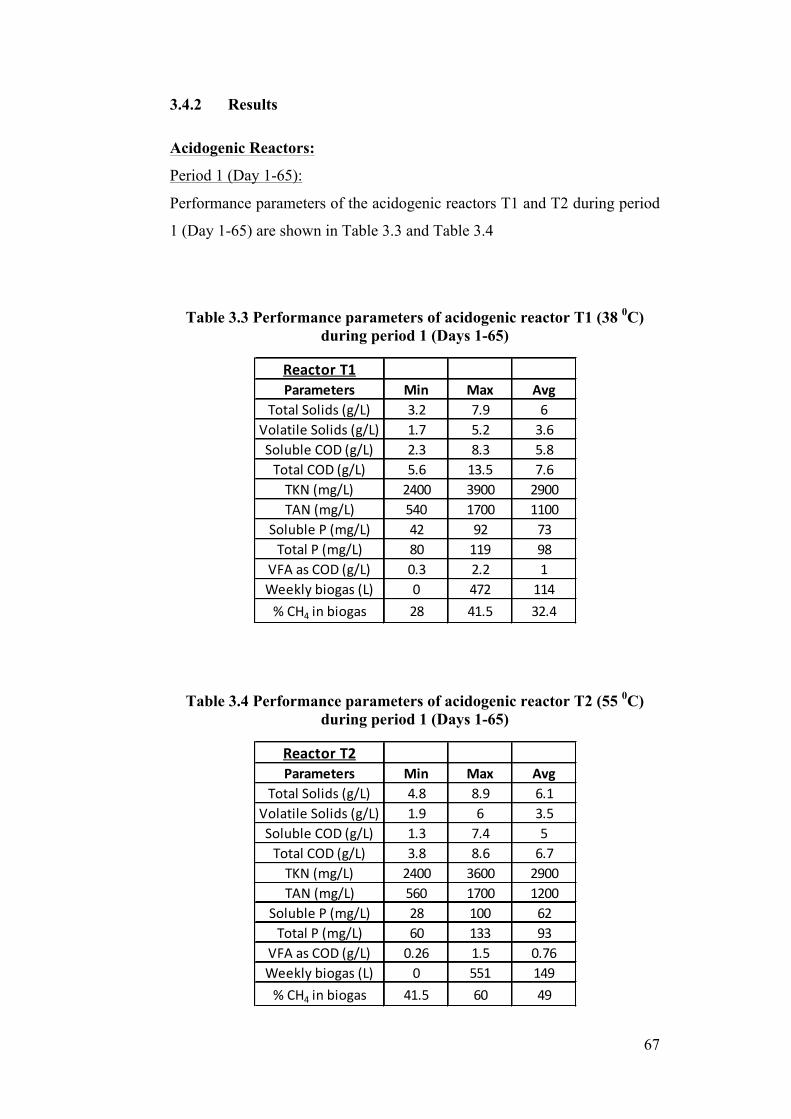
67

3.4.2 Results

Acidogenic Reactors:

Period 1 (Day 1-65):

Performance parameters of the acidogenic reactors T1 and T2 during period

1 (Day 1-65) are shown in Table 3.3 and Table 3.4

Table 3.3 Performance parameters of acidogenic reactor T1 (38 0C) during period 1 (Days 1-65)

Table 3.4 Performance parameters of acidogenic reactor T2 (55 0C) during period 1 (Days 1-65)

Reactor T1Parameters Min Max Avg

Total Solids (g/L) 3.2 7.9 6Volatile Solids (g/L) 1.7 5.2 3.6Soluble COD (g/L) 2.3 8.3 5.8Total COD (g/L) 5.6 13.5 7.6TKN (mg/L) 2400 3900 2900TAN (mg/L) 540 1700 1100

Soluble P (mg/L) 42 92 73Total P (mg/L) 80 119 98

VFA as COD (g/L) 0.3 2.2 1Weekly biogas (L) 0 472 114% CH4 in biogas 28 41.5 32.4


Total Solids (g/L) 4.8 8.9 6.1Volatile Solids (g/L) 1.9 6 3.5Soluble COD (g/L) 1.3 7.4 5Total COD (g/L) 3.8 8.6 6.7TKN (mg/L) 2400 3600 2900TAN (mg/L) 560 1700 1200


VFA as COD (g/L) 0.26 1.5 0.76Weekly biogas (L) 0 551 149% CH4 in biogas 41.5 60 49

68

Performance of the acidification process is measured by the increased

production of VFA’s, as well as solubilisation of organic compounds which

is indicated by an increase in the concentration of soluble COD. During

period 1 (65 day experimental period), both the thermophilic and mesophilic

reactors showed a variable trend in pH during the acidification of the

piggery effluents as shown in Figure 3.9. Initially pH decreased due to

acidification of the effluent, the methanogenic activity following it resulted

in an upward trend in the pH value. The pH increase can be explained by a

drop in the organic loading rate (due to the dilute nature of the raw piggery

effluent) that led to sustained methanogenic activity in both the reactors.

The percentage of soluble COD in both reactors T1 and T2 were 78% and

74% (expressed as a percentage of Total COD in the effluent). Total COD

in the raw piggery effluent was approximately 18.2 g/L of which 68% was

present in the soluble form. The OLR during this period was approximately

2.7 g COD/L/day. Reduction in TCOD and SCOD was calculated to be 53%

and 58% respectively for reactor T1 and 60% and 63% for reactor T2.

VFA levels in reactors T1 and T2 remained around 1 g/L due to VFA’s

being consumed during the process which indicates a stable methanogenic

activity in the reactors as shown in Figure 3.10. The VFA level in both the

reactors reached concentrations over 2 g/L on day 53 due to an increase in

the OLR from 0.64 to 2.4 g COD/L/day over a 2-week period from day 44.

The VFA level then stabilised to below 1 g COD/L/day due to re-

establishment of methanogens even as the OLR remained steady at 2.4 g

COD/L/day.

TKN levels in both reactors reached 2900 mg/L, which was approximately

88% of the TKN level in the raw piggery effluent. TAN levels in reactors

T1 and T2 were 38% and 41% of the TKN in the effluent. Soluble P levels

in reactors T1 and T2 were 74% and 66% of the Total P. Trends of TKN,

TAN and phosphorus in the reactor effluent are shown in Figure 3.11,

Figure 3.12, Figure 3.13 and Figure 3.14.

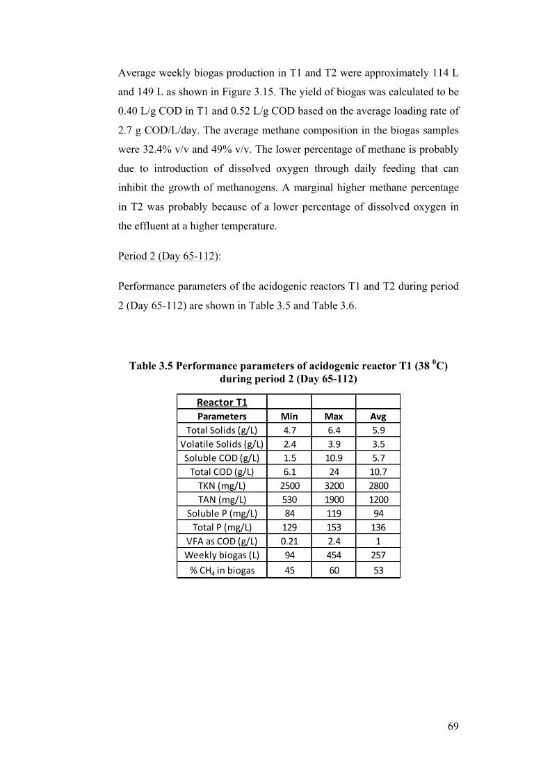
69

Average weekly biogas production in T1 and T2 were approximately 114 L

and 149 L as shown in Figure 3.15. The yield of biogas was calculated to be

0.40 L/g COD in T1 and 0.52 L/g COD based on the average loading rate of

2.7 g COD/L/day. The average methane composition in the biogas samples

were 32.4% v/v and 49% v/v. The lower percentage of methane is probably

due to introduction of dissolved oxygen through daily feeding that can

inhibit the growth of methanogens. A marginal higher methane percentage

in T2 was probably because of a lower percentage of dissolved oxygen in

the effluent at a higher temperature.

Period 2 (Day 65-112):

Performance parameters of the acidogenic reactors T1 and T2 during period

2 (Day 65-112) are shown in Table 3.5 and Table 3.6.

Table 3.5 Performance parameters of acidogenic reactor T1 (38 0C) during period 2 (Day 65-112)


Total Solids (g/L) 4.7 6.4 5.9Volatile Solids (g/L) 2.4 3.9 3.5Soluble COD (g/L) 1.5 10.9 5.7Total COD (g/L) 6.1 24 10.7TKN (mg/L) 2500 3200 2800TAN (mg/L) 530 1900 1200


VFA as COD (g/L) 0.21 2.4 1Weekly biogas (L) 94 454 257% CH4 in biogas 45 60 53

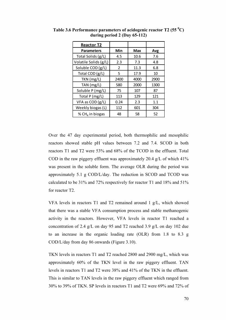
70

Table 3.6 Performance parameters of acidogenic reactor T2 (55 0C) during period 2 (Day 65-112)

Over the 47 day experimental period, both thermophilic and mesophilic

reactors showed stable pH values between 7.2 and 7.4. SCOD in both

reactors T1 and T2 were 53% and 68% of the TCOD in the effluent. Total

COD in the raw piggery effluent was approximately 20.4 g/L of which 41%

was present in the soluble form. The average OLR during the period was

approximately 5.1 g COD/L/day. The reduction in SCOD and TCOD was

calculated to be 31% and 72% respectively for reactor T1 and 18% and 51%

for reactor T2.

VFA levels in reactors T1 and T2 remained around 1 g/L, which showed

that there was a stable VFA consumption process and stable methanogenic

activity in the reactors. However, VFA levels in reactor T1 reached a

concentration of 2.4 g/L on day 95 and T2 reached 3.9 g/L on day 102 due

to an increase in the organic loading rate (OLR) from 1.8 to 8.3 g

COD/L/day from day 86 onwards (Figure 3.10).

TKN levels in reactors T1 and T2 reached 2800 and 2900 mg/L, which was

approximately 60% of the TKN level in the raw piggery effluent. TAN

levels in reactors T1 and T2 were 38% and 41% of the TKN in the effluent.

This is similar to TAN levels in the raw piggery effluent which ranged from

30% to 39% of TKN. SP levels in reactors T1 and T2 were 69% and 72% of


Total Solids (g/L) 4.5 10.6 7.6Volatile Solids (g/L) 2.3 7.3 4.8Soluble COD (g/L) 2 11.3 6.8Total COD (g/L) 5 17.9 10TKN (mg/L) 2400 4000 2900TAN (mg/L) 580 2000 1300


VFA as COD (g/L) 0.24 2.3 1.1Weekly biogas (L) 112 601 304% CH4 in biogas 48 58 52

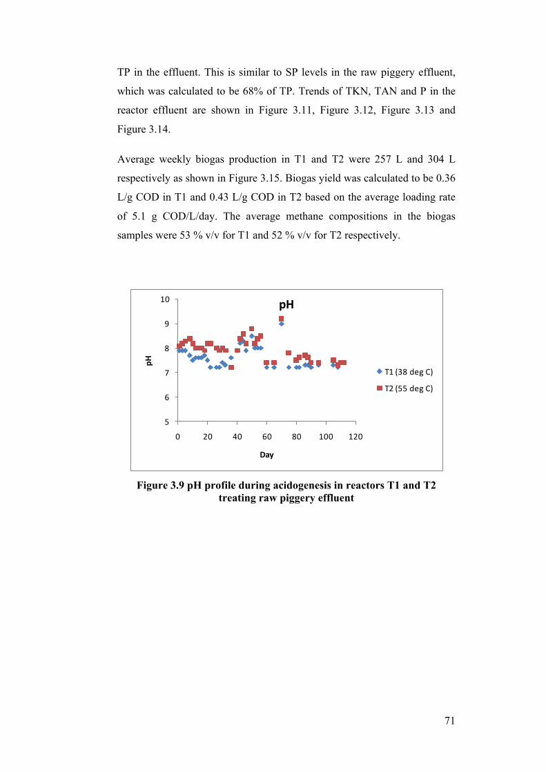
71

TP in the effluent. This is similar to SP levels in the raw piggery effluent,

which was calculated to be 68% of TP. Trends of TKN, TAN and P in the

reactor effluent are shown in Figure 3.11, Figure 3.12, Figure 3.13 and

Figure 3.14.

Average weekly biogas production in T1 and T2 were 257 L and 304 L

respectively as shown in Figure 3.15. Biogas yield was calculated to be 0.36

L/g COD in T1 and 0.43 L/g COD in T2 based on the average loading rate

of 5.1 g COD/L/day. The average methane compositions in the biogas

samples were 53 % v/v for T1 and 52 % v/v for T2 respectively.

Figure 3.9 pH profile during acidogenesis in reactors T1 and T2

treating raw piggery effluent

5

6

7

8

9

10

0 20 40 60 80 100 120

pH

Day

pH

T1 (38 deg C)

T2 (55 deg C)

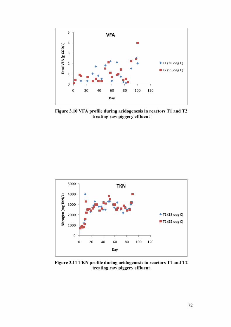
72

Figure 3.10 VFA profile during acidogenesis in reactors T1 and T2


Figure 3.11 TKN profile during acidogenesis in reactors T1 and T2


0

1

2

3

4

5

0 20 40 60 80 100 120

Total V

FA (g COD/

L)

Day

VFA

T1 (38 deg C)

T2 (55 deg C)

0

1000

2000

3000

4000

5000

0 20 40 60 80 100 120

Nitrogen

(mg TKN/L)

Day

TKN

T1 (38 deg C)

T2 (55 deg C)

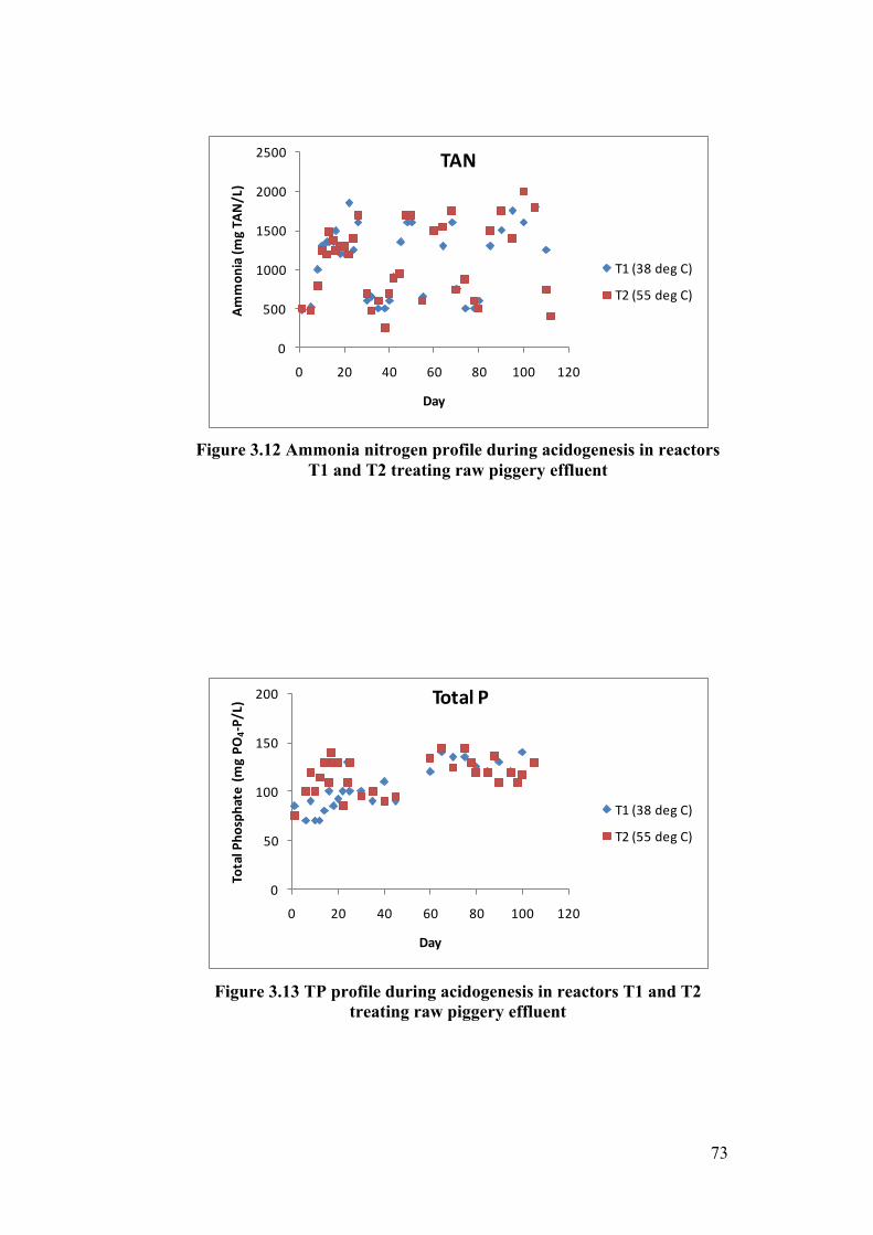
73

Figure 3.12 Ammonia nitrogen profile during acidogenesis in reactors

T1 and T2 treating raw piggery effluent

Figure 3.13 TP profile during acidogenesis in reactors T1 and T2


0

500

1000

1500

2000

2500

0 20 40 60 80 100 120

Ammon

ia (m

g TA

N/L)

Day

TAN

T1 (38 deg C)

T2 (55 deg C)

0

50

100

150

200

0 20 40 60 80 100 120

Total Pho

sphate (m

g PO

4-‐P/L)

Day

Total P

T1 (38 deg C)

T2 (55 deg C)

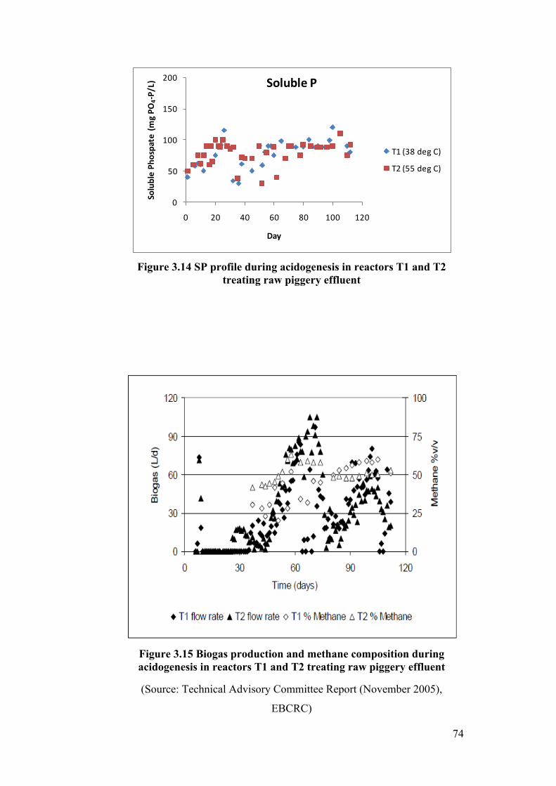
74

Figure 3.14 SP profile during acidogenesis in reactors T1 and T2


Figure 3.15 Biogas production and methane composition during acidogenesis in reactors T1 and T2 treating raw piggery effluent

(Source: Technical Advisory Committee Report (November 2005),

EBCRC)

0

50

100

150

200

0 20 40 60 80 100 120

Soluble Ph

ospate (m

g PO

4-‐P/L)

Day

Soluble P

T1 (38 deg C)

T2 (55 deg C)

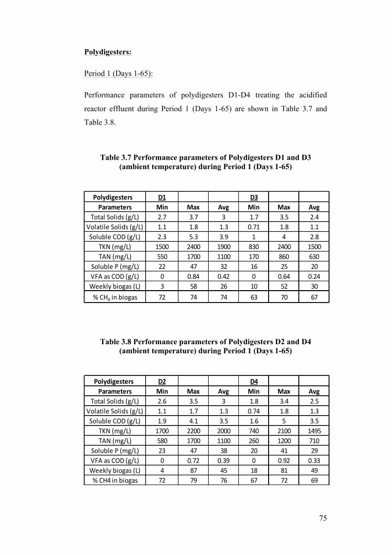
75

Polydigesters:

Period 1 (Days 1-65):

Performance parameters of polydigesters D1-D4 treating the acidified

reactor effluent during Period 1 (Days 1-65) are shown in Table 3.7 and

Table 3.8.

Table 3.7 Performance parameters of Polydigesters D1 and D3 (ambient temperature) during Period 1 (Days 1-65)


Polydigesters D1 D3Parameters Min Max Avg Min Max Avg

Total Solids (g/L) 2.7 3.7 3 1.7 3.5 2.4Volatile Solids (g/L) 1.1 1.8 1.3 0.71 1.8 1.1Soluble COD (g/L) 2.3 5.3 3.9 1 4 2.8

TKN (mg/L) 1500 2400 1900 830 2400 1500TAN (mg/L) 550 1700 1100 170 860 630

Soluble P (mg/L) 22 47 32 16 25 20VFA as COD (g/L) 0 0.84 0.42 0 0.64 0.24Weekly biogas (L) 3 58 26 10 52 30% CH4 in biogas 72 74 74 63 70 67


Total Solids (g/L) 2.6 3.5 3 1.8 3.4 2.5Volatile Solids (g/L) 1.1 1.7 1.3 0.74 1.8 1.3Soluble COD (g/L) 1.9 4.1 3.5 1.6 5 3.5

TKN (mg/L) 1700 2200 2000 740 2100 1495TAN (mg/L) 580 1700 1100 260 1200 710


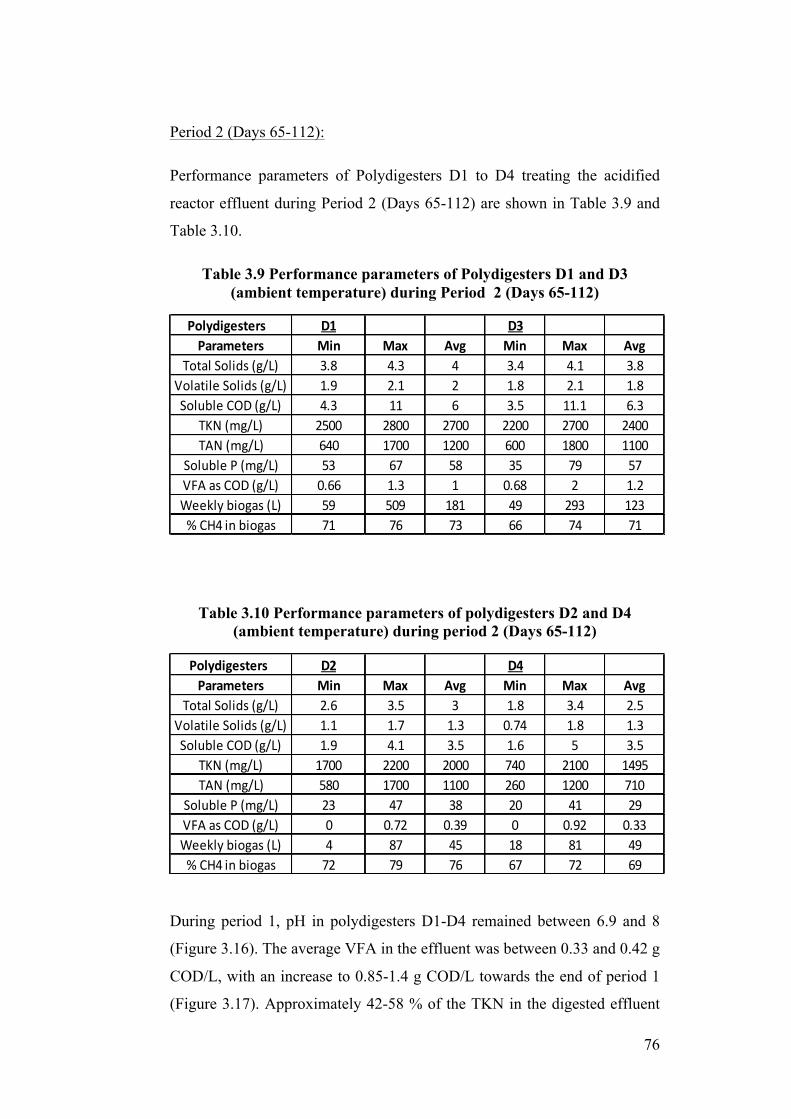
76

Period 2 (Days 65-112):

Performance parameters of Polydigesters D1 to D4 treating the acidified

reactor effluent during Period 2 (Days 65-112) are shown in Table 3.9 and

Table 3.10.


Table 3.10 Performance parameters of polydigesters D2 and D4 (ambient temperature) during period 2 (Days 65-112)

During period 1, pH in polydigesters D1-D4 remained between 6.9 and 8

(Figure 3.16). The average VFA in the effluent was between 0.33 and 0.42 g

COD/L, with an increase to 0.85-1.4 g COD/L towards the end of period 1

(Figure 3.17). Approximately 42-58 % of the TKN in the digested effluent


Total Solids (g/L) 3.8 4.3 4 3.4 4.1 3.8Volatile Solids (g/L) 1.9 2.1 2 1.8 2.1 1.8Soluble COD (g/L) 4.3 11 6 3.5 11.1 6.3

TKN (mg/L) 2500 2800 2700 2200 2700 2400TAN (mg/L) 640 1700 1200 600 1800 1100

Soluble P (mg/L) 53 67 58 35 79 57VFA as COD (g/L) 0.66 1.3 1 0.68 2 1.2Weekly biogas (L) 59 509 181 49 293 123% CH4 in biogas 71 76 73 66 74 71


Total Solids (g/L) 2.6 3.5 3 1.8 3.4 2.5Volatile Solids (g/L) 1.1 1.7 1.3 0.74 1.8 1.3Soluble COD (g/L) 1.9 4.1 3.5 1.6 5 3.5

TKN (mg/L) 1700 2200 2000 740 2100 1495TAN (mg/L) 580 1700 1100 260 1200 710


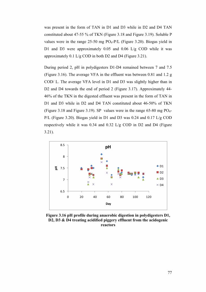
77

was present in the form of TAN in D1 and D3 while in D2 and D4 TAN

constituted about 47-55 % of TKN (Figure 3.18 and Figure 3.19). Soluble P

values were in the range 25-50 mg PO4-P/L (Figure 3.20). Biogas yield in

D1 and D3 were approximately 0.05 and 0.06 L/g COD while it was

approximately 0.1 L/g COD in both D2 and D4 (Figure 3.21).

During period 2, pH in polydigesters D1-D4 remained between 7 and 7.5

(Figure 3.16). The average VFA in the effluent was between 0.81 and 1.2 g

COD/ L. The average VFA level in D1 and D3 was slightly higher than in

D2 and D4 towards the end of period 2 (Figure 3.17). Approximately 44-

46% of the TKN in the digested effluent was present in the form of TAN in

D1 and D3 while in D2 and D4 TAN constituted about 46-50% of TKN

(Figure 3.18 and Figure 3.19). SP values were in the range 65-80 mg PO4-

P/L (Figure 3.20). Biogas yield in D1 and D3 was 0.24 and 0.17 L/g COD

respectively while it was 0.34 and 0.32 L/g COD in D2 and D4 (Figure

3.21).

Figure 3.16 pH profile during anaerobic digestion in polydigesters D1,

D2, D3 & D4 treating acidified piggery effluent from the acidogenic reactors

6.5

7

7.5

8

8.5

0 20 40 60 80 100 120

pH

Day

pH

D1

D2

D3

D4

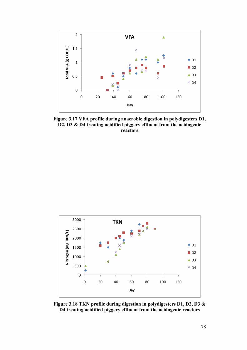
78

Figure 3.17 VFA profile during anaerobic digestion in polydigesters D1,

D2, D3 & D4 treating acidified piggery effluent from the acidogenic reactors

Figure 3.18 TKN profile during digestion in polydigesters D1, D2, D3 &

D4 treating acidified piggery effluent from the acidogenic reactors

0

0.5

1

1.5

2

0 20 40 60 80 100 120

Total V

FA (g COD/

L)

Day

VFA

D1

D2

D3

D4

0

500

1000

1500

2000

2500

3000

0 20 40 60 80 100 120

Nitrogen

(mg TKN/L)

Day

TKN

D1

D2

D3

D4

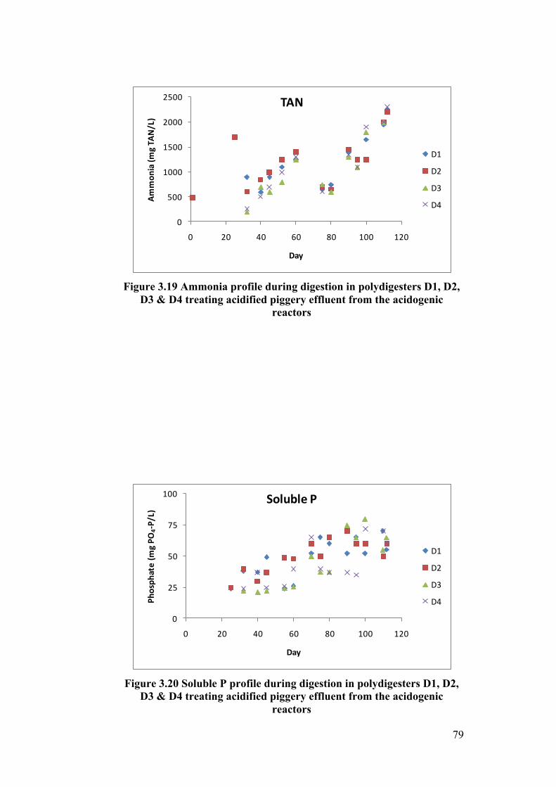
79

Figure 3.19 Ammonia profile during digestion in polydigesters D1, D2,

D3 & D4 treating acidified piggery effluent from the acidogenic reactors

Figure 3.20 Soluble P profile during digestion in polydigesters D1, D2,

D3 & D4 treating acidified piggery effluent from the acidogenic reactors

0

500

1000

1500

2000

2500

0 20 40 60 80 100 120

Ammon

ia (m

g TA

N/L)

Day

TAN

D1

D2

D3

D4

0

25

50

75

100

0 20 40 60 80 100 120

Phosph

ate (m

g PO

4-‐P/L)

Day

Soluble P

D1

D2

D3

D4

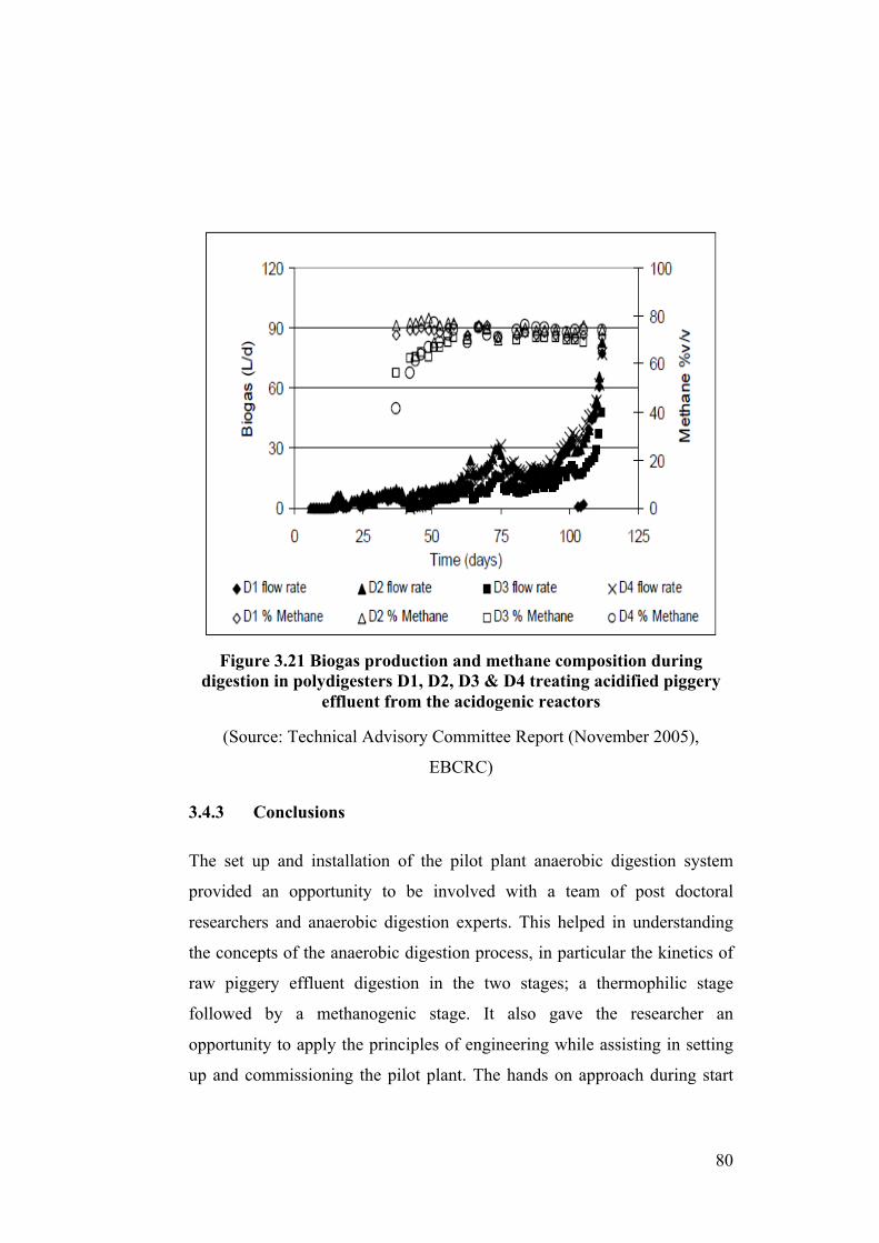
80

Figure 3.21 Biogas production and methane composition during

digestion in polydigesters D1, D2, D3 & D4 treating acidified piggery effluent from the acidogenic reactors

(Source: Technical Advisory Committee Report (November 2005),

EBCRC)

3.4.3 Conclusions

The set up and installation of the pilot plant anaerobic digestion system

provided an opportunity to be involved with a team of post doctoral

researchers and anaerobic digestion experts. This helped in understanding

the concepts of the anaerobic digestion process, in particular the kinetics of

raw piggery effluent digestion in the two stages; a thermophilic stage

followed by a methanogenic stage. It also gave the researcher an

opportunity to apply the principles of engineering while assisting in setting

up and commissioning the pilot plant. The hands on approach during start

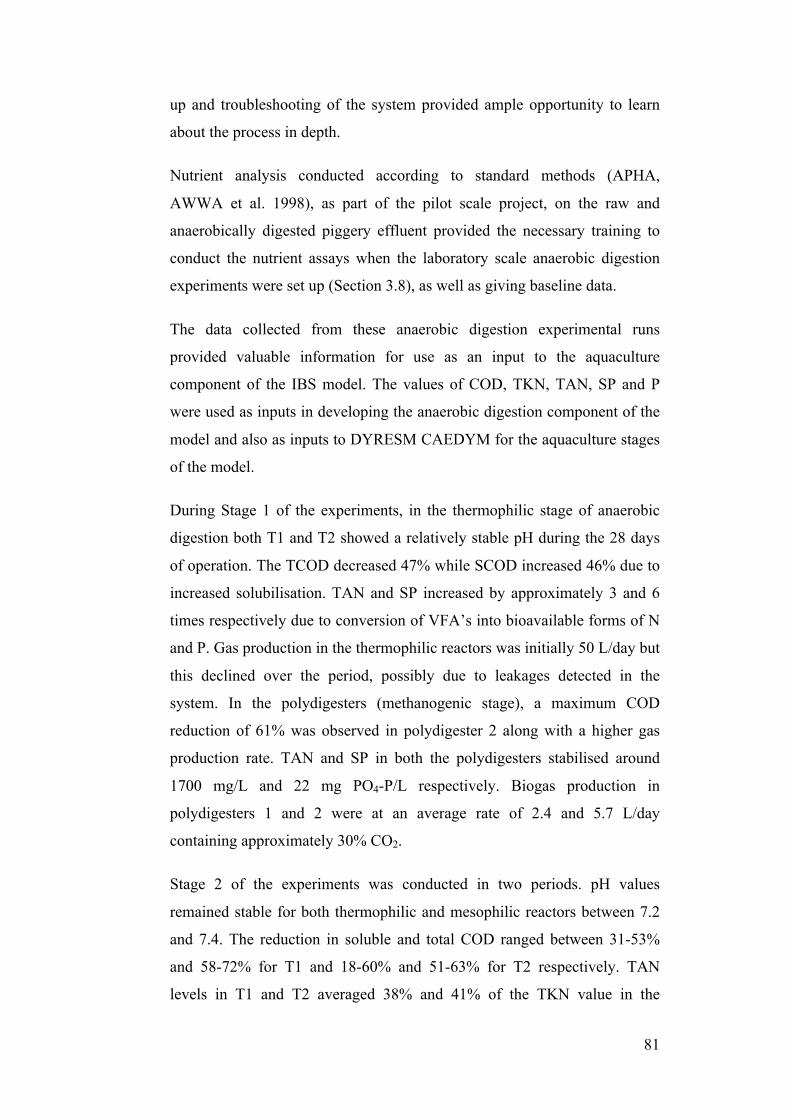
81

up and troubleshooting of the system provided ample opportunity to learn

about the process in depth.

Nutrient analysis conducted according to standard methods (APHA,

AWWA et al. 1998), as part of the pilot scale project, on the raw and

anaerobically digested piggery effluent provided the necessary training to

conduct the nutrient assays when the laboratory scale anaerobic digestion

experiments were set up (Section 3.8), as well as giving baseline data.

The data collected from these anaerobic digestion experimental runs

provided valuable information for use as an input to the aquaculture

component of the IBS model. The values of COD, TKN, TAN, SP and P

were used as inputs in developing the anaerobic digestion component of the

model and also as inputs to DYRESM CAEDYM for the aquaculture stages

of the model.

During Stage 1 of the experiments, in the thermophilic stage of anaerobic

digestion both T1 and T2 showed a relatively stable pH during the 28 days

of operation. The TCOD decreased 47% while SCOD increased 46% due to

increased solubilisation. TAN and SP increased by approximately 3 and 6

times respectively due to conversion of VFA’s into bioavailable forms of N

and P. Gas production in the thermophilic reactors was initially 50 L/day but

this declined over the period, possibly due to leakages detected in the

system. In the polydigesters (methanogenic stage), a maximum COD

reduction of 61% was observed in polydigester 2 along with a higher gas

production rate. TAN and SP in both the polydigesters stabilised around

1700 mg/L and 22 mg PO4-P/L respectively. Biogas production in

polydigesters 1 and 2 were at an average rate of 2.4 and 5.7 L/day

containing approximately 30% CO2.

Stage 2 of the experiments was conducted in two periods. pH values

remained stable for both thermophilic and mesophilic reactors between 7.2

and 7.4. The reduction in soluble and total COD ranged between 31-53%

and 58-72% for T1 and 18-60% and 51-63% for T2 respectively. TAN

levels in T1 and T2 averaged 38% and 41% of the TKN value in the

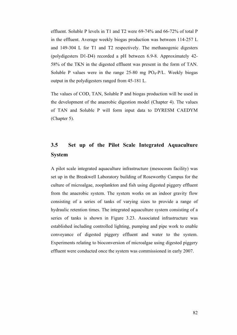
82

effluent. Soluble P levels in T1 and T2 were 69-74% and 66-72% of total P

in the effluent. Average weekly biogas production was between 114-257 L

and 149-304 L for T1 and T2 respectively. The methanogenic digesters

(polydigesters D1-D4) recorded a pH between 6.9-8. Approximately 42-

58% of the TKN in the digested effluent was present in the form of TAN.

Soluble P values were in the range 25-80 mg PO4-P/L. Weekly biogas

output in the polydigesters ranged from 45-181 L.

The values of COD, TAN, Soluble P and biogas production will be used in

the development of the anaerobic digestion model (Chapter 4). The values

of TAN and Soluble P will form input data to DYRESM CAEDYM

(Chapter 5).

3.5 Set up of the Pilot Scale Integrated Aquaculture

System

A pilot scale integrated aquaculture infrastructure (mesocosm facility) was

set up in the Breakwell Laboratory building of Roseworthy Campus for the

culture of microalgae, zooplankton and fish using digested piggery effluent

from the anaerobic system. The system works on an indoor gravity flow

consisting of a series of tanks of varying sizes to provide a range of

hydraulic retention times. The integrated aquaculture system consisting of a

series of tanks is shown in Figure 3.23. Associated infrastructure was

established including controlled lighting, pumping and pipe work to enable

conveyance of digested piggery effluent and water to the system.

Experiments relating to bioconversion of microalgae using digested piggery

effluent were conducted once the system was commissioned in early 2007.

83

Figure 3.22 Schematic diagram of the pilot scale Integrated Aquaculture System

Figure 3.23 Clear Perspex tanks set up at differential heights for micro-algal culture while blue fibre glass tanks are used for fish culture. These tanks are part of the indoor integrated aquaculture system (mesocosm)

at Roseworthy Laboratory

Microalgae

Zooplankton

Fish

Anaerobically digested

piggery effluent

84

3.6 Bioconversion of piggery effluent to algae (280 L

working volume)

3.6.1 Objective

The aim of this experiment was to evaluate the bioconversion of algae

Chlorella sp. at a fixed working volume of 280 L and a nutrient

concentration of 30 mg/L/day of TAN. This was achieved by the addition of

anaerobically digested piggery effluent as the nutrient source. The data of

TAN, SP and pH obtained from these experiments were used to model the

zooplankton component of DYRESM CAEDYM for the IBS model.

3.6.2 Materials and Methods

Three 400 L photo bioreactors were used each with a total working volume

of 280 L. The reactors were filled with 280 L of dechlorinated mains water.

The reactors were inoculated with Chlorella sp. (10%), which was obtained

from the microalgal laboratory at the University of Adelaide. The

experiment was conducted under controlled fluorescent light (45000 Lux)

and 15:9 hours photoperiod (light: dark) at 24 0C. The concentration of

nutrient in the reactors were maintained above 30 mg/L TAN by daily

addition of anaerobically digested piggery effluent. The effluent had a TAN

of 1646 mg/L and soluble orthophosphate of 55.2 mg/L. Samples of culture

were collected daily. The samples were analysed for total algal cell density,

and nutrient concentrations (ammonia and soluble orthophosphate). Nutrient

analysis was conducted according to the APHA et al., Standard Methods

(1998). The cell density was measured using a haemocytometer and a

binocular microscope. Once the cell density reached 2.5 million cells/mL,

the algal culture was diluted to 1.0 million cells/mL by harvesting the algae

and making up the volume to 280 L by addition of dechlorinated water. pH,

temperature and DO were monitored daily. pH was maintained above 9.5 to

minimize risk of infestation by rotifers into the system. The algae removed

from these reactors were used as an inoculum for the start up of three other

algal reactors.

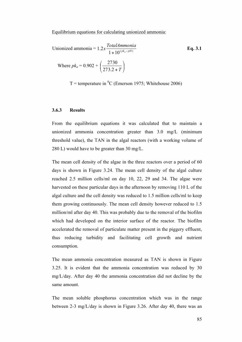
85

Equilibrium equations for calculating unionized ammonia:

Unionized ammonia = )(101

2.1 pHpka

iaTotalAmmonx−+

Eq. 3.1

Where pka = 0.902 + ⎟⎠

⎞⎜⎝

⎛+T2.273

2730

T = temperature in 0C (Emerson 1975; Whitehouse 2006)

3.6.3 Results

From the equilibrium equations it was calculated that to maintain a

unionized ammonia concentration greater than 3.0 mg/L (minimum

threshold value), the TAN in the algal reactors (with a working volume of

280 L) would have to be greater than 30 mg/L.

The mean cell density of the algae in the three reactors over a period of 60

days is shown in Figure 3.24. The mean cell density of the algal culture

reached 2.5 million cells/ml on day 10, 22, 29 and 34. The algae were

harvested on these particular days in the afternoon by removing 110 L of the

algal culture and the cell density was reduced to 1.5 million cells/ml to keep

them growing continuously. The mean cell density however reduced to 1.5

million/ml after day 40. This was probably due to the removal of the biofilm

which had developed on the interior surface of the reactor. The biofilm

accelerated the removal of particulate matter present in the piggery effluent,

thus reducing turbidity and facilitating cell growth and nutrient

consumption.

The mean ammonia concentration measured as TAN is shown in Figure

3.25. It is evident that the ammonia concentration was reduced by 30

mg/L/day. After day 40 the ammonia concentration did not decline by the

same amount.

The mean soluble phosphorus concentration which was in the range

between 2-3 mg/L/day is shown in Figure 3.26. After day 40, there was an

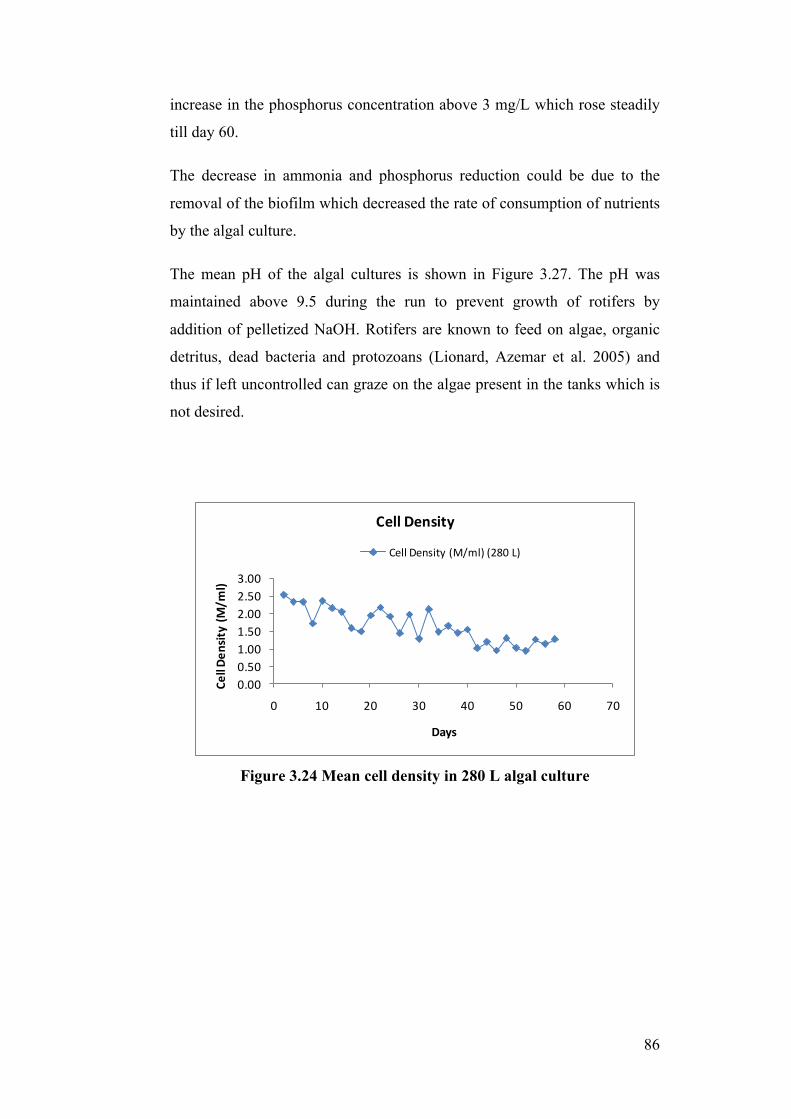
86

increase in the phosphorus concentration above 3 mg/L which rose steadily

till day 60.

The decrease in ammonia and phosphorus reduction could be due to the

removal of the biofilm which decreased the rate of consumption of nutrients

by the algal culture.

The mean pH of the algal cultures is shown in Figure 3.27. The pH was

maintained above 9.5 during the run to prevent growth of rotifers by

addition of pelletized NaOH. Rotifers are known to feed on algae, organic

detritus, dead bacteria and protozoans (Lionard, Azemar et al. 2005) and

thus if left uncontrolled can graze on the algae present in the tanks which is

not desired.

Figure 3.24 Mean cell density in 280 L algal culture

0.000.501.001.502.002.503.00

0 10 20 30 40 50 60 70

Cell D

ensity (M

/ml)

Days

Cell Density

Cell Density (M/ml) (280 L)

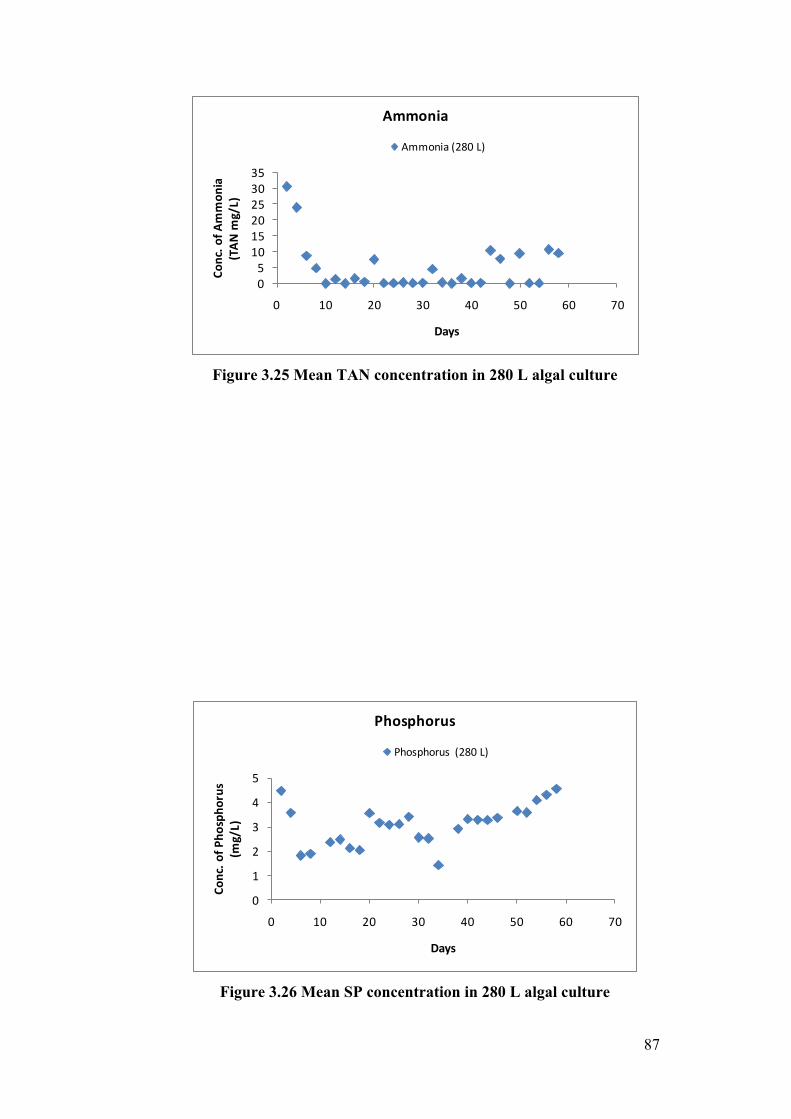
87

Figure 3.25 Mean TAN concentration in 280 L algal culture

Figure 3.26 Mean SP concentration in 280 L algal culture

05101520253035

0 10 20 30 40 50 60 70

Conc. o

f Ammon

ia(TAN

mg/L)

Days

Ammonia

Ammonia (280 L)

0

1

2

3

4

5

0 10 20 30 40 50 60 70

Conc. o

f Pho

spho

rus

(mg/L)

Days

Phosphorus

Phosphorus (280 L)

88

Figure 3.27 Mean pH in 280 L algal culture

3.6.4 Key findings

• The daily average cell production rate was 0.15 million cells/mL.

• The mean nutrient consumption was 30 mg/L/day of TAN over 60

days.

• The pH of the algal culture was maintained above 9.5 and the

unionized ammonia concentration was greater than 3.0 mg/L.

• The experiment was run for 60 days successfully without infestation

by rotifers.

3.7 Bioconversion of piggery effluent to algae (180 L

working volume)

3.7.1 Objective

The aim of this experiment was to evaluate the bioconversion of algae

Chlorella spp. at a fixed working volume of 180 L and at a fixed nutrient

concentration of 30 mg/L/day of TAN by the addition of anaerobically

digested piggery effluent as the nutrient source.

67

89

1011

12

0 10 20 30 40 50 60 70

pH

Days

pH

pH (280 L)

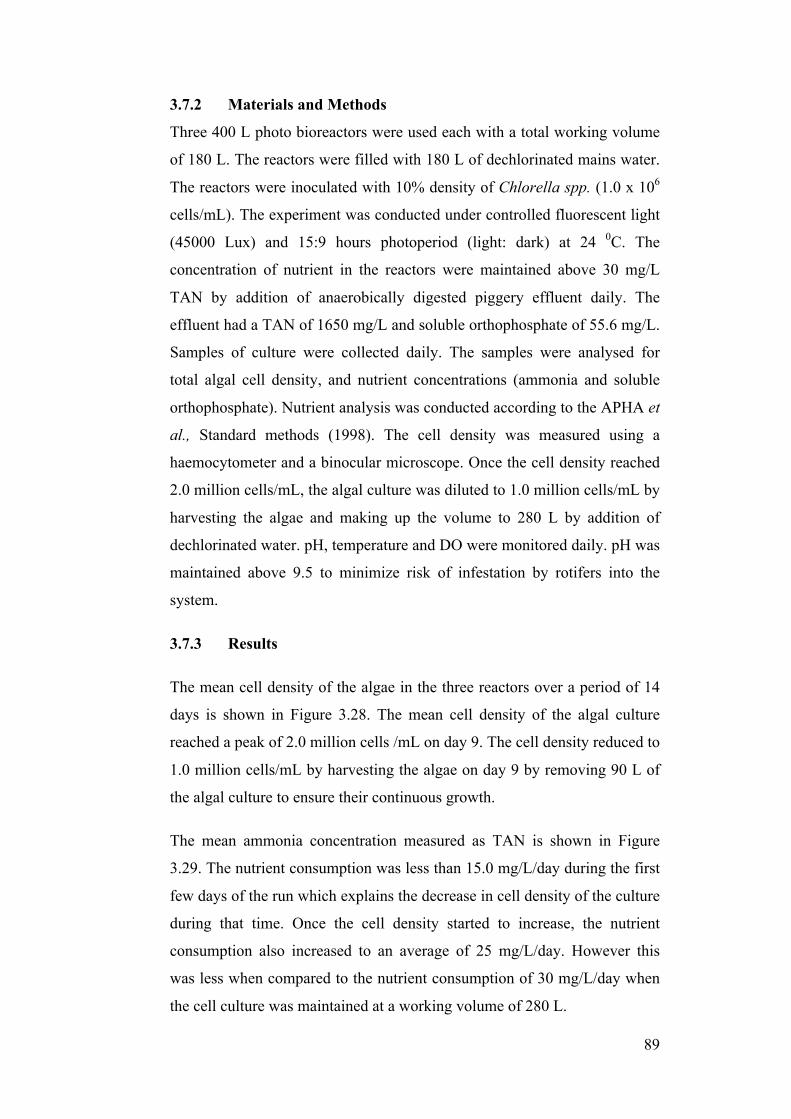
89

3.7.2 Materials and Methods

Three 400 L photo bioreactors were used each with a total working volume

of 180 L. The reactors were filled with 180 L of dechlorinated mains water.

The reactors were inoculated with 10% density of Chlorella spp. (1.0 x 106

cells/mL). The experiment was conducted under controlled fluorescent light

(45000 Lux) and 15:9 hours photoperiod (light: dark) at 24 0C. The

concentration of nutrient in the reactors were maintained above 30 mg/L

TAN by addition of anaerobically digested piggery effluent daily. The

effluent had a TAN of 1650 mg/L and soluble orthophosphate of 55.6 mg/L.

Samples of culture were collected daily. The samples were analysed for

total algal cell density, and nutrient concentrations (ammonia and soluble

orthophosphate). Nutrient analysis was conducted according to the APHA et

al., Standard methods (1998). The cell density was measured using a

haemocytometer and a binocular microscope. Once the cell density reached

2.0 million cells/mL, the algal culture was diluted to 1.0 million cells/mL by

harvesting the algae and making up the volume to 280 L by addition of

dechlorinated water. pH, temperature and DO were monitored daily. pH was

maintained above 9.5 to minimize risk of infestation by rotifers into the

system.

3.7.3 Results

The mean cell density of the algae in the three reactors over a period of 14

days is shown in Figure 3.28. The mean cell density of the algal culture

reached a peak of 2.0 million cells /mL on day 9. The cell density reduced to

1.0 million cells/mL by harvesting the algae on day 9 by removing 90 L of

the algal culture to ensure their continuous growth.

The mean ammonia concentration measured as TAN is shown in Figure

3.29. The nutrient consumption was less than 15.0 mg/L/day during the first

few days of the run which explains the decrease in cell density of the culture

during that time. Once the cell density started to increase, the nutrient

consumption also increased to an average of 25 mg/L/day. However this

was less when compared to the nutrient consumption of 30 mg/L/day when

the cell culture was maintained at a working volume of 280 L.

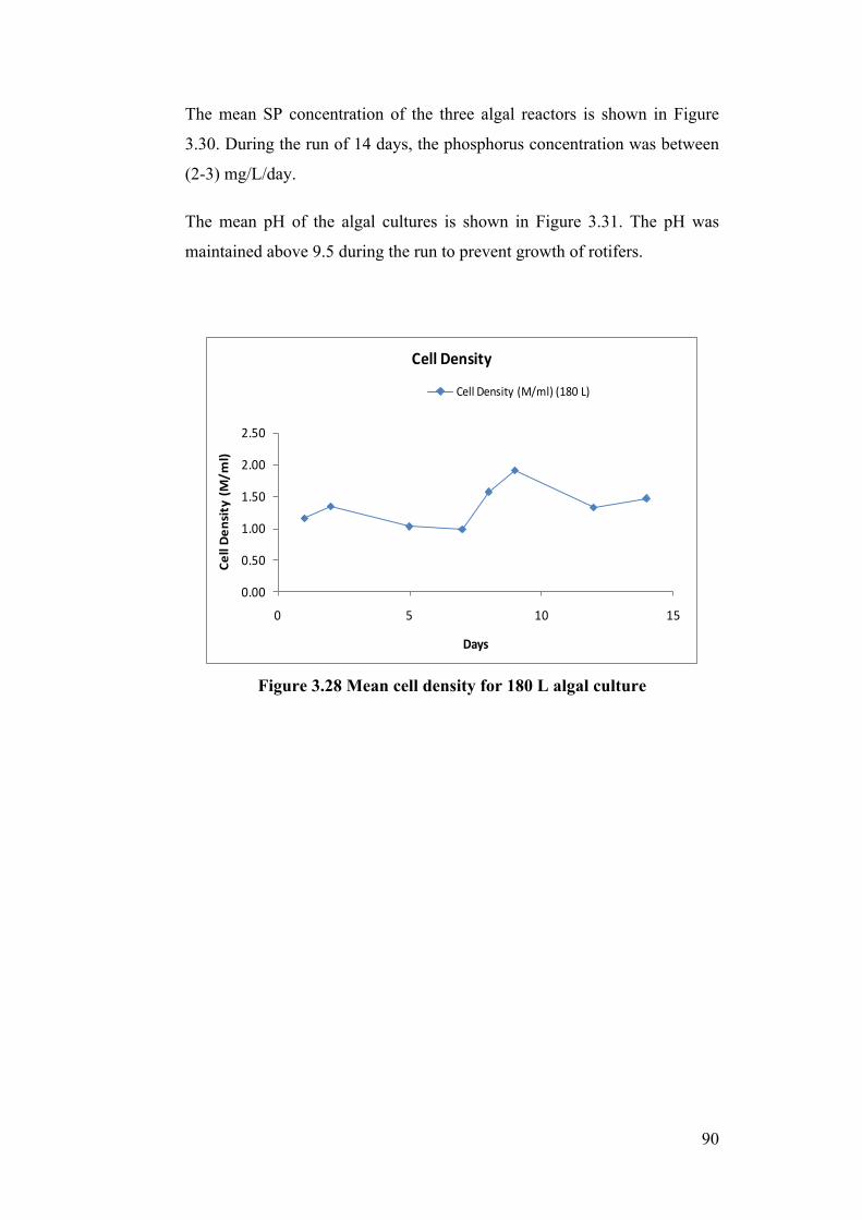
90

The mean SP concentration of the three algal reactors is shown in Figure

3.30. During the run of 14 days, the phosphorus concentration was between

(2-3) mg/L/day.

The mean pH of the algal cultures is shown in Figure 3.31. The pH was

maintained above 9.5 during the run to prevent growth of rotifers.

Figure 3.28 Mean cell density for 180 L algal culture

0.00

0.50

1.00

1.50

2.00

2.50

0 5 10 15

Cell Den

sity (M/m

l)

Days

Cell Density

Cell Density (M/ml) (180 L)

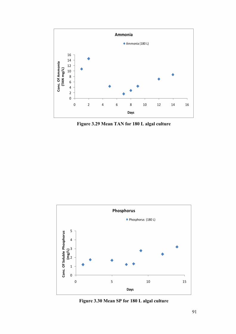
91

Figure 3.29 Mean TAN for 180 L algal culture

Figure 3.30 Mean SP for 180 L algal culture

02468

10121416

0 2 4 6 8 10 12 14 16

Conc. O

f Ammon

ia

(TAN m

g/L)

Days

Ammonia

Ammonia (180 L)

0

1

2

3

4

5

0 5 10 15

Conc. O

f Solub

le Pho

spho

rus

(mg/L)

Days

Phosphorus

Phosphorus (180 L)

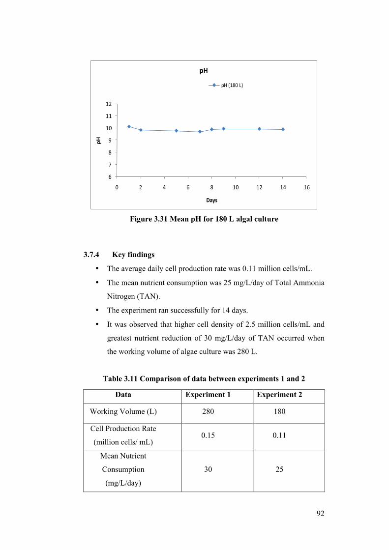
92

Figure 3.31 Mean pH for 180 L algal culture

3.7.4 Key findings

• The average daily cell production rate was 0.11 million cells/mL.

• The mean nutrient consumption was 25 mg/L/day of Total Ammonia

Nitrogen (TAN).

• The experiment ran successfully for 14 days.

• It was observed that higher cell density of 2.5 million cells/mL and

greatest nutrient reduction of 30 mg/L/day of TAN occurred when

the working volume of algae culture was 280 L.

Table 3.11 Comparison of data between experiments 1 and 2

Data Experiment 1 Experiment 2

Working Volume (L) 280 180

Cell Production Rate

(million cells/ mL) 0.15 0.11

Mean Nutrient

Consumption

(mg/L/day)

30 25

6

7

8

9

10

11

12

0 2 4 6 8 10 12 14 16

pH

Days

pH

pH (180 L)

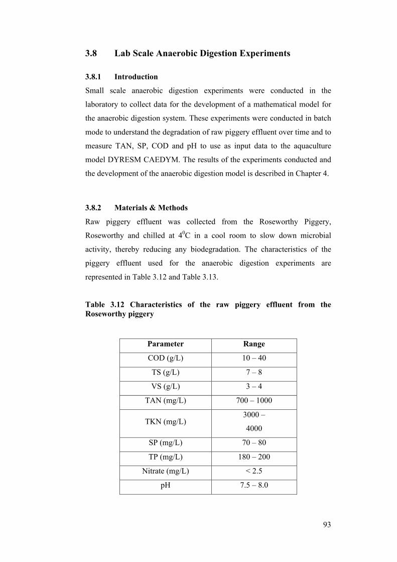
93

3.8 Lab Scale Anaerobic Digestion Experiments

3.8.1 Introduction

Small scale anaerobic digestion experiments were conducted in the

laboratory to collect data for the development of a mathematical model for

the anaerobic digestion system. These experiments were conducted in batch

mode to understand the degradation of raw piggery effluent over time and to

measure TAN, SP, COD and pH to use as input data to the aquaculture

model DYRESM CAEDYM. The results of the experiments conducted and

the development of the anaerobic digestion model is described in Chapter 4.

3.8.2 Materials & Methods

Raw piggery effluent was collected from the Roseworthy Piggery,

Roseworthy and chilled at 40C in a cool room to slow down microbial

activity, thereby reducing any biodegradation. The characteristics of the

piggery effluent used for the anaerobic digestion experiments are

represented in Table 3.12 and Table 3.13.

Table 3.12 Characteristics of the raw piggery effluent from the Roseworthy piggery

Parameter Range

COD (g/L) 10 – 40

TS (g/L) 7 – 8

VS (g/L) 3 – 4

TAN (mg/L) 700 – 1000

TKN (mg/L) 3000 –

4000

SP (mg/L) 70 – 80

TP (mg/L) 180 – 200

Nitrate (mg/L) < 2.5

pH 7.5 – 8.0

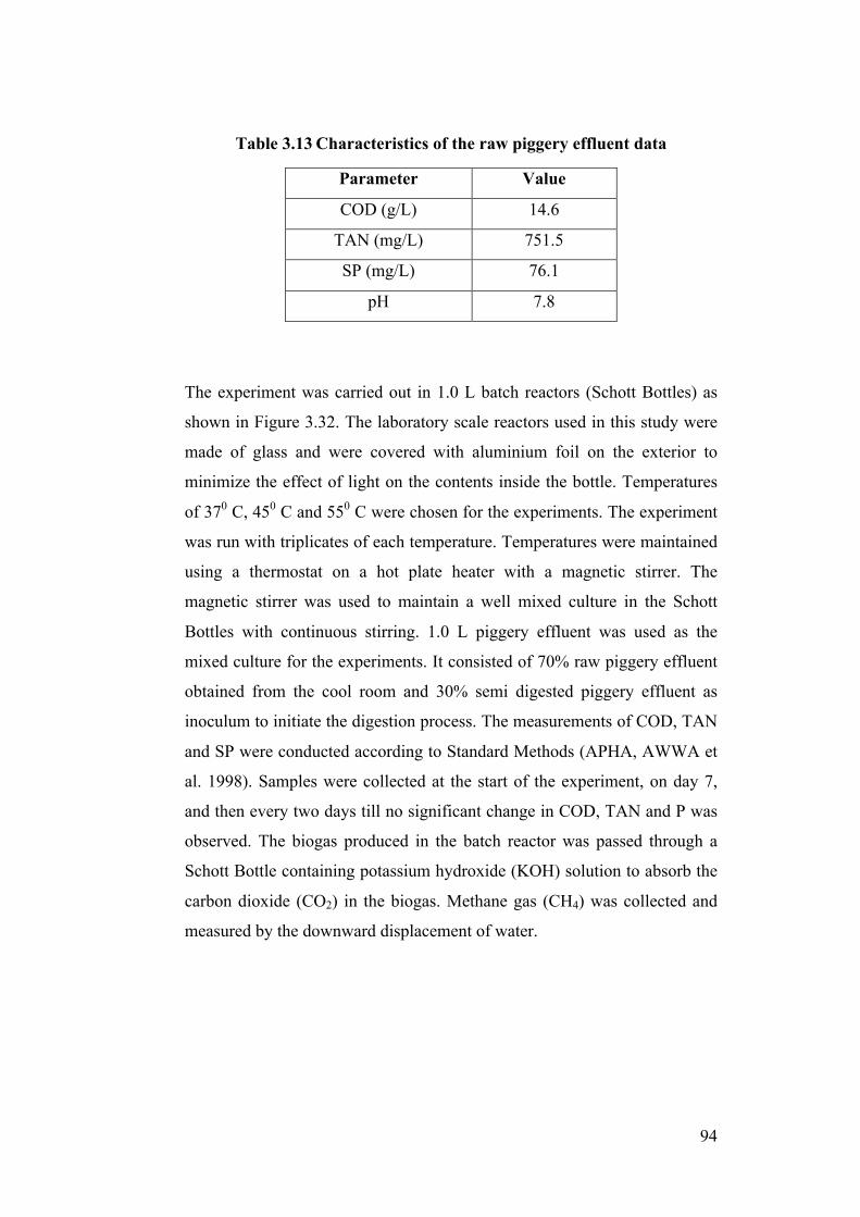
94

Table 3.13 Characteristics of the raw piggery effluent data

Parameter Value

COD (g/L) 14.6

TAN (mg/L) 751.5

SP (mg/L) 76.1

pH 7.8

The experiment was carried out in 1.0 L batch reactors (Schott Bottles) as

shown in Figure 3.32. The laboratory scale reactors used in this study were

made of glass and were covered with aluminium foil on the exterior to

minimize the effect of light on the contents inside the bottle. Temperatures

of 370 C, 450 C and 550 C were chosen for the experiments. The experiment

was run with triplicates of each temperature. Temperatures were maintained

using a thermostat on a hot plate heater with a magnetic stirrer. The

magnetic stirrer was used to maintain a well mixed culture in the Schott

Bottles with continuous stirring. 1.0 L piggery effluent was used as the

mixed culture for the experiments. It consisted of 70% raw piggery effluent

obtained from the cool room and 30% semi digested piggery effluent as

inoculum to initiate the digestion process. The measurements of COD, TAN

and SP were conducted according to Standard Methods (APHA, AWWA et

al. 1998). Samples were collected at the start of the experiment, on day 7,

and then every two days till no significant change in COD, TAN and P was

observed. The biogas produced in the batch reactor was passed through a

Schott Bottle containing potassium hydroxide (KOH) solution to absorb the

carbon dioxide (CO2) in the biogas. Methane gas (CH4) was collected and

measured by the downward displacement of water.

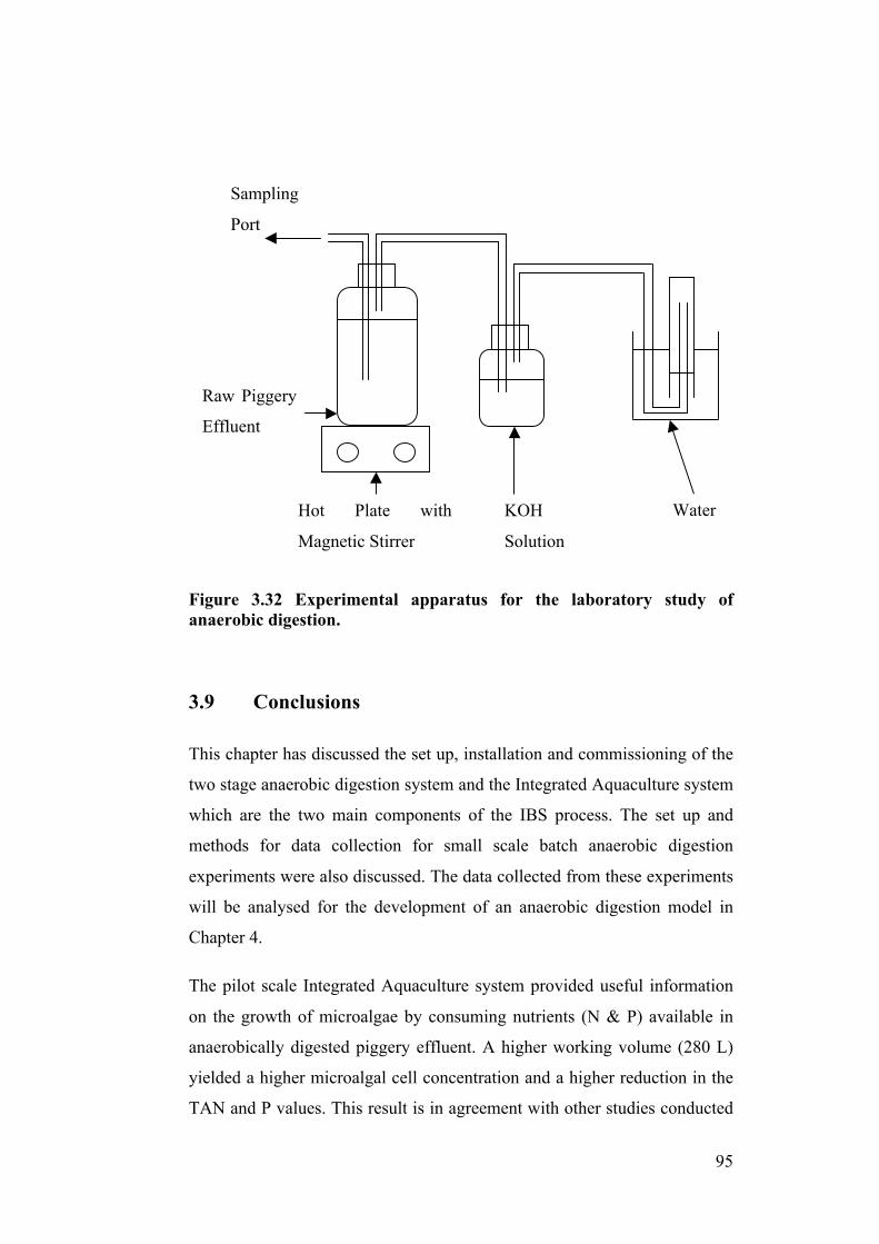
95

Figure 3.32 Experimental apparatus for the laboratory study of anaerobic digestion.

3.9 Conclusions

This chapter has discussed the set up, installation and commissioning of the

two stage anaerobic digestion system and the Integrated Aquaculture system

which are the two main components of the IBS process. The set up and

methods for data collection for small scale batch anaerobic digestion

experiments were also discussed. The data collected from these experiments

will be analysed for the development of an anaerobic digestion model in

Chapter 4.

The pilot scale Integrated Aquaculture system provided useful information

on the growth of microalgae by consuming nutrients (N & P) available in

anaerobically digested piggery effluent. A higher working volume (280 L)

yielded a higher microalgal cell concentration and a higher reduction in the

TAN and P values. This result is in agreement with other studies conducted

Sampling

Port

Raw Piggery

Effluent

KOH

Solution

Hot Plate with

Magnetic Stirrer

Water

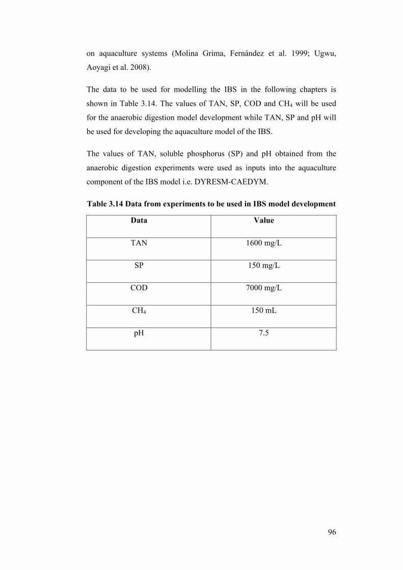
96

on aquaculture systems (Molina Grima, Fernández et al. 1999; Ugwu,

Aoyagi et al. 2008).

The data to be used for modelling the IBS in the following chapters is

shown in Table 3.14. The values of TAN, SP, COD and CH4 will be used

for the anaerobic digestion model development while TAN, SP and pH will

be used for developing the aquaculture model of the IBS.

The values of TAN, soluble phosphorus (SP) and pH obtained from the

anaerobic digestion experiments were used as inputs into the aquaculture

component of the IBS model i.e. DYRESM-CAEDYM.

Table 3.14 Data from experiments to be used in IBS model development

Data Value

TAN 1600 mg/L

SP 150 mg/L

COD 7000 mg/L

CH4 150 mL

pH 7.5

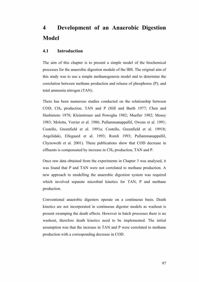
97

4 Development of an Anaerobic Digestion

Model

4.1 Introduction

The aim of this chapter is to present a simple model of the biochemical

processes for the anaerobic digestion module of the IBS. The original aim of

this study was to use a simple methanogenesis model and to determine the

correlation between methane production and release of phosphorus (P); and

total ammonia nitrogen (TAN).

There has been numerous studies conducted on the relationship between

COD, CH4 production, TAN and P (Hill and Barth 1977; Chen and

Hashimoto 1978; Kleinstreuer and Powegha 1982; Mueller 1982; Mosey

1983; Moletta, Verrier et al. 1986; Pullammanappallil, Owens et al. 1991;

Costello, Greenfield et al. 1991a; Costello, Greenfield et al. 1991b;

Angelidaki, Ellegaard et al. 1993; Romli 1993; Pullammanappallil,

Chynoweth et al. 2001). These publications show that COD decrease in

effluents is compensated by increase in CH4 production, TAN and P.

Once raw data obtained from the experiments in Chapter 3 was analysed, it

was found that P and TAN were not correlated to methane production. A

new approach to modelling the anaerobic digestion system was required

which involved separate microbial kinetics for TAN, P and methane

production.

Conventional anaerobic digesters operate on a continuous basis. Death

kinetics are not incorporated in continuous digester models as washout is

present swamping the death effects. However in batch processes there is no

washout, therefore death kinetics need to be implemented. The initial

assumption was that the increase in TAN and P were correlated to methane

production with a corresponding decrease in COD.

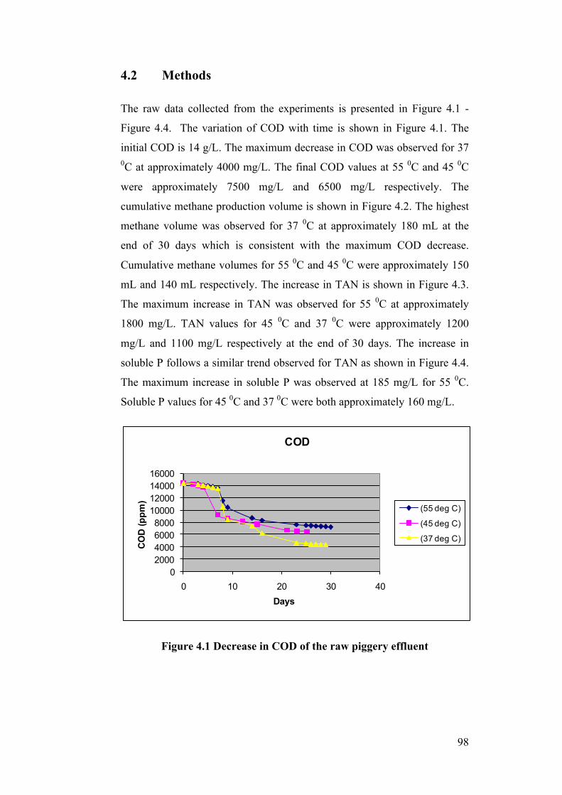
98

4.2 Methods

The raw data collected from the experiments is presented in Figure 4.1 -

Figure 4.4. The variation of COD with time is shown in Figure 4.1. The

initial COD is 14 g/L. The maximum decrease in COD was observed for 37 0C at approximately 4000 mg/L. The final COD values at 55 0C and 45 0C

were approximately 7500 mg/L and 6500 mg/L respectively. The

cumulative methane production volume is shown in Figure 4.2. The highest

methane volume was observed for 37 0C at approximately 180 mL at the

end of 30 days which is consistent with the maximum COD decrease.

Cumulative methane volumes for 55 0C and 45 0C were approximately 150

mL and 140 mL respectively. The increase in TAN is shown in Figure 4.3.

The maximum increase in TAN was observed for 55 0C at approximately

1800 mg/L. TAN values for 45 0C and 37 0C were approximately 1200

mg/L and 1100 mg/L respectively at the end of 30 days. The increase in

soluble P follows a similar trend observed for TAN as shown in Figure 4.4.

The maximum increase in soluble P was observed at 185 mg/L for 55 0C.

Soluble P values for 45 0C and 37 0C were both approximately 160 mg/L.

Figure 4.1 Decrease in COD of the raw piggery effluent

02000400060008000

10000120001400016000

0 10 20 30 40

COD

(ppm

)

Days

COD

(55 deg C)

(45 deg C)

(37 deg C)

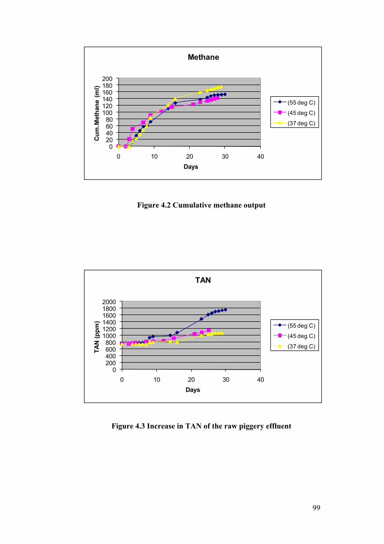
99

Figure 4.2 Cumulative methane output

Figure 4.3 Increase in TAN of the raw piggery effluent

020406080

100120140160180200

0 10 20 30 40

Cum

.Met

hane

(ml)

Days

Methane

(55 deg C)

(45 deg C)

(37 deg C)

0200400600800

100012001400160018002000

0 10 20 30 40

TAN

(ppm

)

Days

TAN

(55 deg C)

(45 deg C)

(37 deg C)

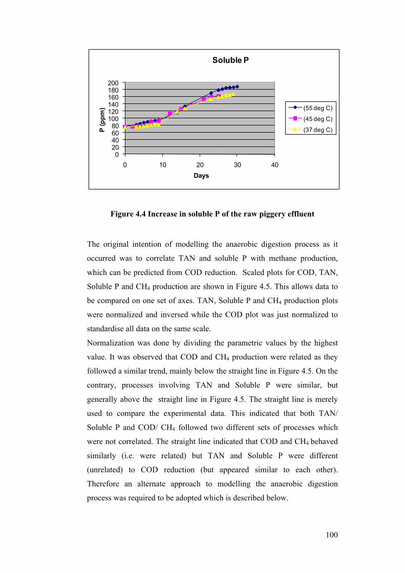
100

Figure 4.4 Increase in soluble P of the raw piggery effluent

The original intention of modelling the anaerobic digestion process as it

occurred was to correlate TAN and soluble P with methane production,

which can be predicted from COD reduction. Scaled plots for COD, TAN,

Soluble P and CH4 production are shown in Figure 4.5. This allows data to

be compared on one set of axes. TAN, Soluble P and CH4 production plots

were normalized and inversed while the COD plot was just normalized to

standardise all data on the same scale.

Normalization was done by dividing the parametric values by the highest

value. It was observed that COD and CH4 production were related as they

followed a similar trend, mainly below the straight line in Figure 4.5. On the

contrary, processes involving TAN and Soluble P were similar, but

generally above the straight line in Figure 4.5. The straight line is merely

used to compare the experimental data. This indicated that both TAN/

Soluble P and COD/ CH4 followed two different sets of processes which

were not correlated. The straight line indicated that COD and CH4 behaved

similarly (i.e. were related) but TAN and Soluble P were different

(unrelated) to COD reduction (but appeared similar to each other).

Therefore an alternate approach to modelling the anaerobic digestion

process was required to be adopted which is described below.

020406080

100120140160180200

0 10 20 30 40

P (p

pm)

Days

Soluble P

(55 deg C)

(45 deg C)

(37 deg C)

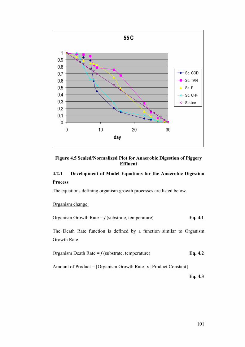
101

Figure 4.5 Scaled/Normalized Plot for Anaerobic Digestion of Piggery Effluent

4.2.1 Development of Model Equations for the Anaerobic Digestion

Process

The equations defining organism growth processes are listed below.

Organism change:

Organism Growth Rate = f (substrate, temperature) Eq. 4.1

The Death Rate function is defined by a function similar to Organism

Growth Rate.

Organism Death Rate = f (substrate, temperature) Eq. 4.2

Amount of Product = [Organism Growth Rate] x [Product Constant]

Eq. 4.3

00.10.20.30.40.50.60.70.80.9

1

0 10 20 30day

55 C

Sc. COD

Sc. TAN

Sc. P

Sc. CH4

StrLine

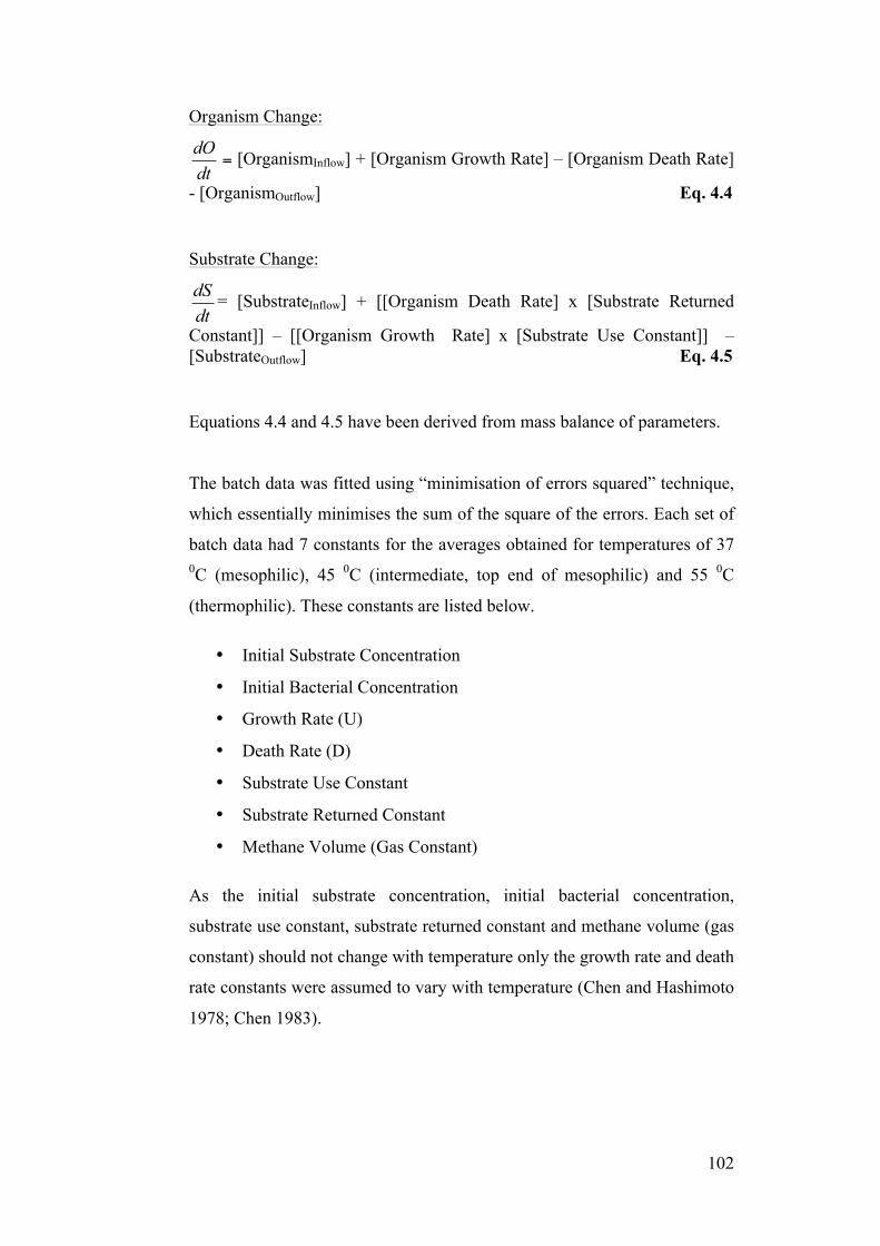
102

Organism Change:

=dtdO

[OrganismInflow] + [Organism Growth Rate] – [Organism Death Rate]

- [OrganismOutflow] Eq. 4.4

Substrate Change:

dtdS = [SubstrateInflow] + [[Organism Death Rate] x [Substrate Returned

Constant]] – [[Organism Growth Rate] x [Substrate Use Constant]] – [SubstrateOutflow] Eq. 4.5

Equations 4.4 and 4.5 have been derived from mass balance of parameters.

The batch data was fitted using “minimisation of errors squared” technique,

which essentially minimises the sum of the square of the errors. Each set of

batch data had 7 constants for the averages obtained for temperatures of 37 0C (mesophilic), 45 0C (intermediate, top end of mesophilic) and 55 0C

(thermophilic). These constants are listed below.

• Initial Substrate Concentration

• Initial Bacterial Concentration

• Growth Rate (U)

• Death Rate (D)

• Substrate Use Constant

• Substrate Returned Constant

• Methane Volume (Gas Constant)

As the initial substrate concentration, initial bacterial concentration,

substrate use constant, substrate returned constant and methane volume (gas

constant) should not change with temperature only the growth rate and death

rate constants were assumed to vary with temperature (Chen and Hashimoto

1978; Chen 1983).

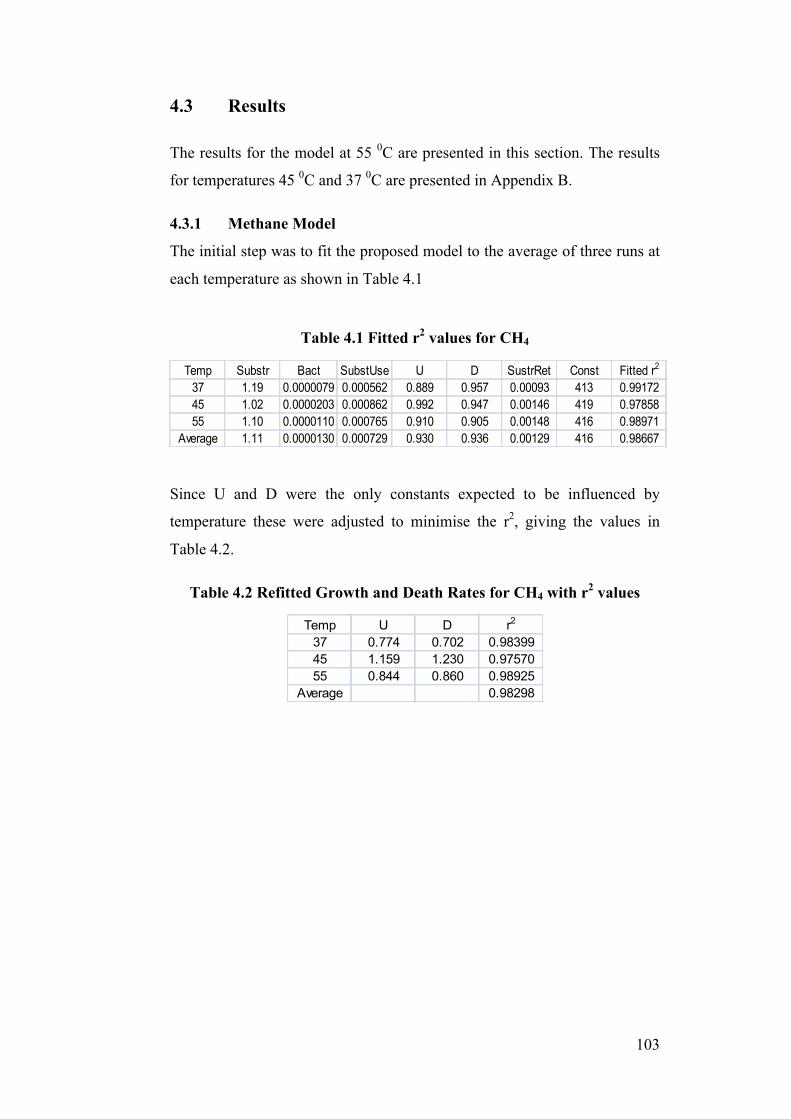
103

4.3 Results

The results for the model at 55 0C are presented in this section. The results

for temperatures 45 0C and 37 0C are presented in Appendix B.

4.3.1 Methane Model

The initial step was to fit the proposed model to the average of three runs at

each temperature as shown in Table 4.1

Table 4.1 Fitted r2 values for CH4

Since U and D were the only constants expected to be influenced by

temperature these were adjusted to minimise the r2, giving the values in

Table 4.2.

Table 4.2 Refitted Growth and Death Rates for CH4 with r2 values

Temp Substr Bact SubstUse U D SustrRet Const Fitted r2

37 1.19 0.0000079 0.000562 0.889 0.957 0.00093 413 0.9917245 1.02 0.0000203 0.000862 0.992 0.947 0.00146 419 0.9785855 1.10 0.0000110 0.000765 0.910 0.905 0.00148 416 0.98971

Average 1.11 0.0000130 0.000729 0.930 0.936 0.00129 416 0.98667

Temp U D r2

37 0.774 0.702 0.9839945 1.159 1.230 0.9757055 0.844 0.860 0.98925

Average 0.98298

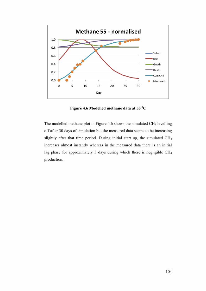
104

Figure 4.6 Modelled methane data at 55 0C

The modelled methane plot in Figure 4.6 shows the simulated CH4 levelling

off after 30 days of simulation but the measured data seems to be increasing

slightly after that time period. During initial start up, the simulated CH4

increases almost instantly whereas in the measured data there is an initial

lag phase for approximately 3 days during which there is negligible CH4

production.

0.0

0.2

0.4

0.6

0.8

1.0

0 5 10 15 20 25 30

Day

Methane 55 -‐ normalised

Substr

Bact

Grwth

Death

Cum CH4

Measured

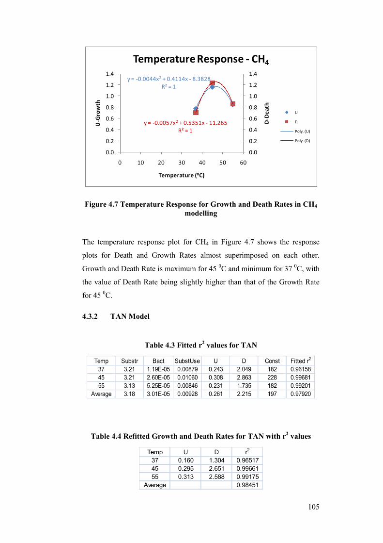
105

Figure 4.7 Temperature Response for Growth and Death Rates in CH4 modelling

The temperature response plot for CH4 in Figure 4.7 shows the response

plots for Death and Growth Rates almost superimposed on each other.

Growth and Death Rate is maximum for 45 0C and minimum for 37 0C, with

the value of Death Rate being slightly higher than that of the Growth Rate

for 45 0C.

4.3.2 TAN Model

Table 4.3 Fitted r2 values for TAN

Table 4.4 Refitted Growth and Death Rates for TAN with r2 values

y = -‐0.0044x2 + 0.4114x -‐ 8.3828R² = 1

y = -‐0.0057x2 + 0.5351x -‐ 11.265R² = 1

0.0

0.2

0.4

0.6

0.8

1.0

1.2

1.4

0.0

0.2

0.4

0.6

0.8

1.0

1.2

1.4

0 10 20 30 40 50 60

D-‐De

ath

U-‐Growth

Temperature (oC)

Temperature Response -‐ CH4

U

D

Poly. (U)

Poly. (D)

Temp Substr Bact SubstUse U D Const Fitted r2

37 3.21 1.19E-05 0.00879 0.243 2.049 182 0.9615845 3.21 2.60E-05 0.01060 0.308 2.863 228 0.9968155 3.13 5.25E-05 0.00846 0.231 1.735 182 0.99201

Average 3.18 3.01E-05 0.00928 0.261 2.215 197 0.97920

Temp U D r2

37 0.160 1.304 0.9651745 0.295 2.651 0.9966155 0.313 2.588 0.99175

Average 0.98451

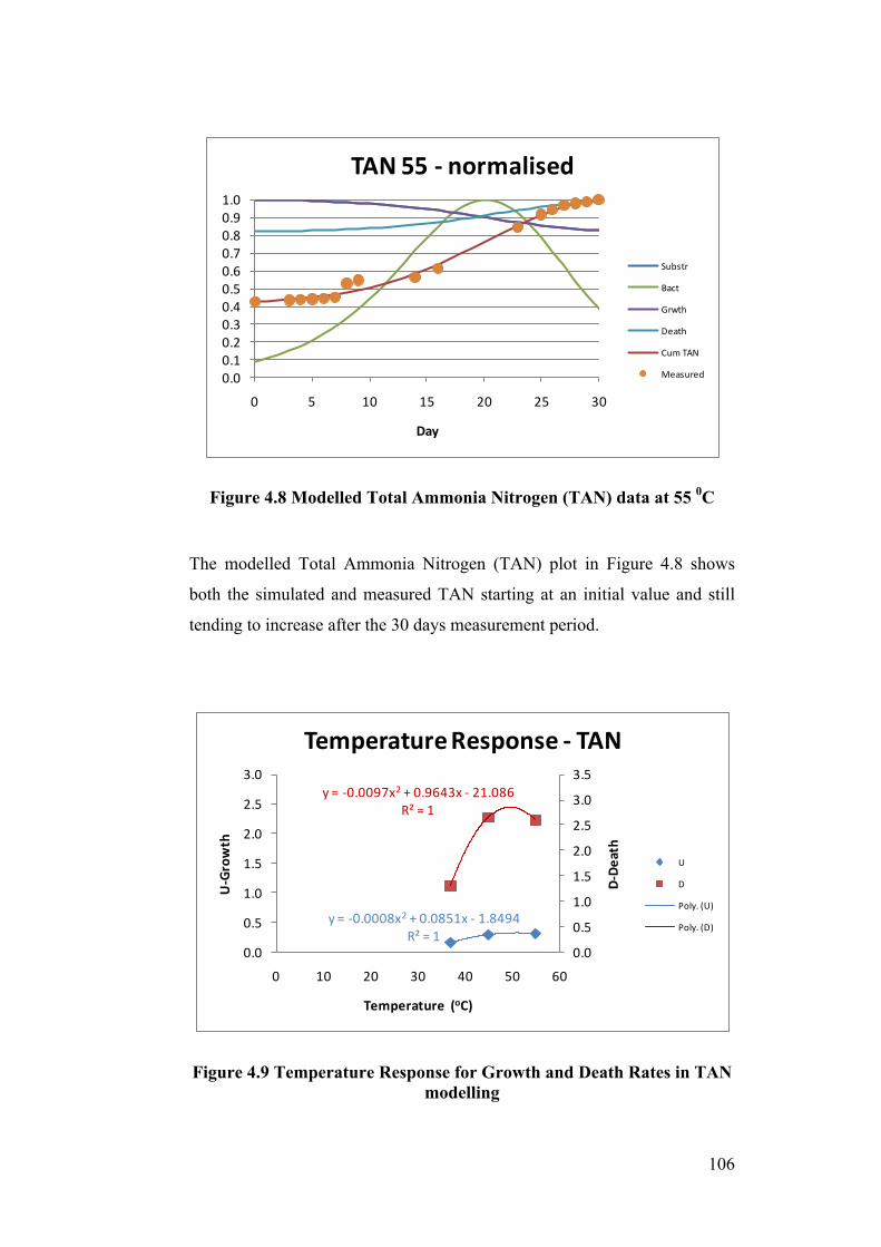
106

Figure 4.8 Modelled Total Ammonia Nitrogen (TAN) data at 55 0C

The modelled Total Ammonia Nitrogen (TAN) plot in Figure 4.8 shows

both the simulated and measured TAN starting at an initial value and still

tending to increase after the 30 days measurement period.

Figure 4.9 Temperature Response for Growth and Death Rates in TAN modelling

0.00.10.20.30.40.50.60.70.80.91.0

0 5 10 15 20 25 30

Day

TAN 55 -‐ normalised

Substr

Bact

Grwth

Death

Cum TAN

Measured

y = -‐0.0008x2 + 0.0851x -‐ 1.8494R² = 1

y = -‐0.0097x2 + 0.9643x -‐ 21.086R² = 1

0.0

0.5

1.0

1.5

2.0

2.5

3.0

3.5

0.0

0.5

1.0

1.5

2.0

2.5

3.0

0 10 20 30 40 50 60

D-‐De

ath

U-‐Growth

Temperature (oC)

Temperature Response -‐ TAN

U

D

Poly. (U)

Poly. (D)

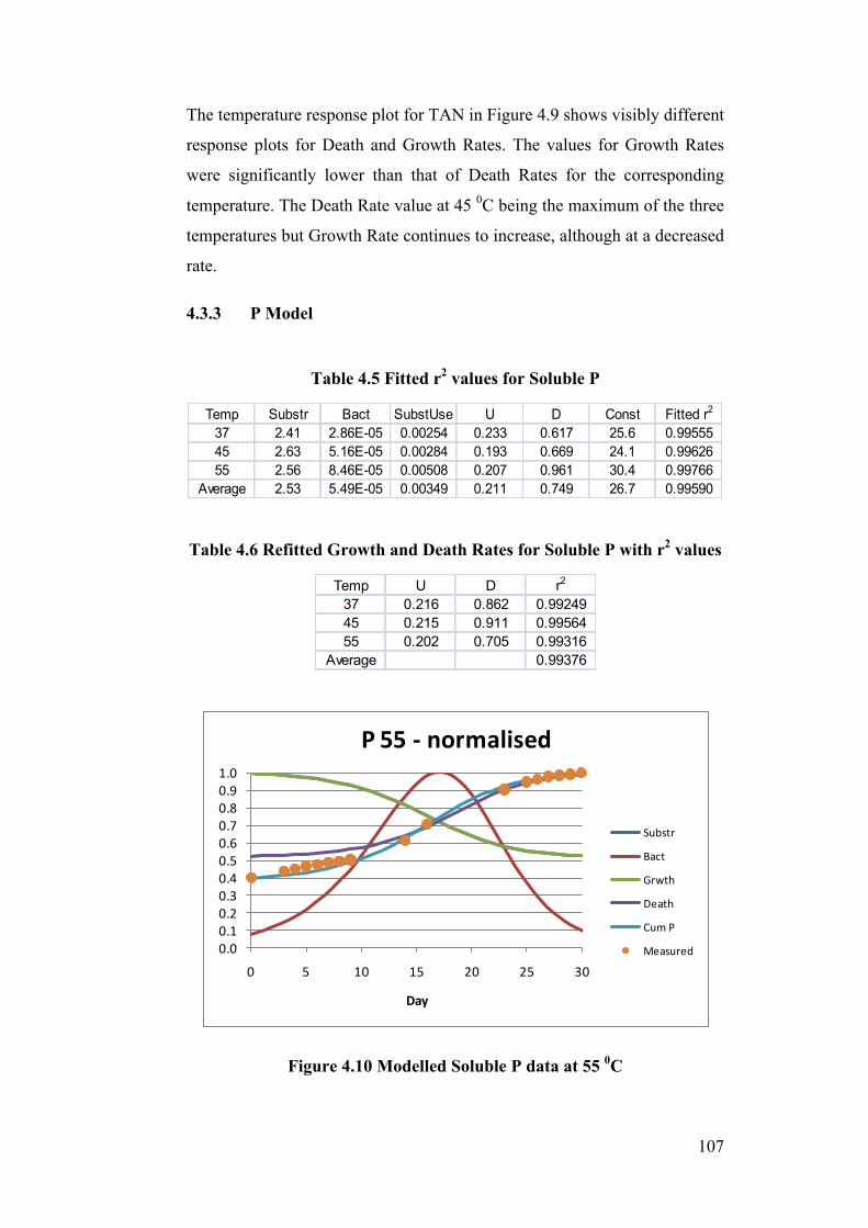
107

The temperature response plot for TAN in Figure 4.9 shows visibly different

response plots for Death and Growth Rates. The values for Growth Rates

were significantly lower than that of Death Rates for the corresponding

temperature. The Death Rate value at 45 0C being the maximum of the three

temperatures but Growth Rate continues to increase, although at a decreased

rate.

4.3.3 P Model

Table 4.5 Fitted r2 values for Soluble P

Table 4.6 Refitted Growth and Death Rates for Soluble P with r2 values

Figure 4.10 Modelled Soluble P data at 55 0C

Temp Substr Bact SubstUse U D Const Fitted r2

37 2.41 2.86E-05 0.00254 0.233 0.617 25.6 0.9955545 2.63 5.16E-05 0.00284 0.193 0.669 24.1 0.9962655 2.56 8.46E-05 0.00508 0.207 0.961 30.4 0.99766

Average 2.53 5.49E-05 0.00349 0.211 0.749 26.7 0.99590

Temp U D r2

37 0.216 0.862 0.9924945 0.215 0.911 0.9956455 0.202 0.705 0.99316

Average 0.99376

0.00.10.20.30.40.50.60.70.80.91.0

0 5 10 15 20 25 30

Day

P 55 -‐ normalised

Substr

Bact

Grwth

Death

Cum P

Measured

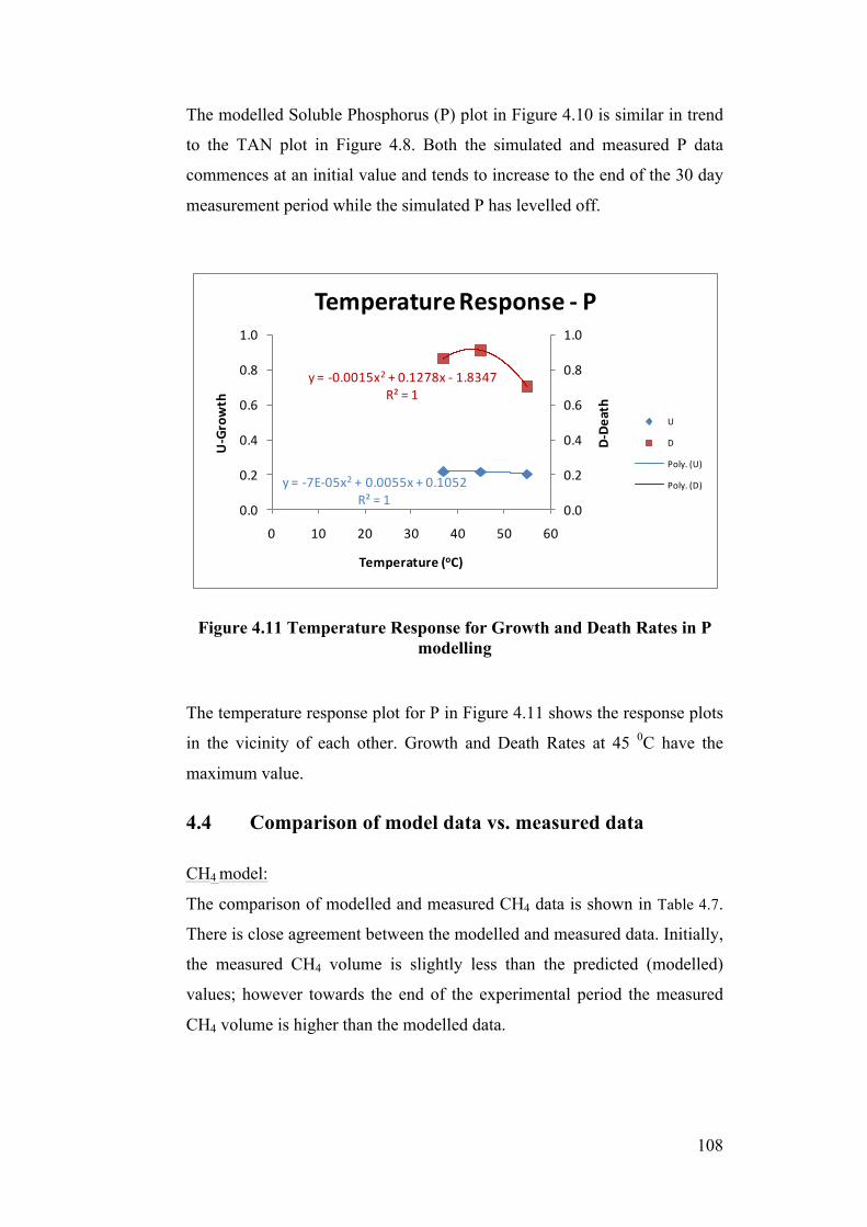
108

The modelled Soluble Phosphorus (P) plot in Figure 4.10 is similar in trend

to the TAN plot in Figure 4.8. Both the simulated and measured P data

commences at an initial value and tends to increase to the end of the 30 day

measurement period while the simulated P has levelled off.

Figure 4.11 Temperature Response for Growth and Death Rates in P modelling

The temperature response plot for P in Figure 4.11 shows the response plots

in the vicinity of each other. Growth and Death Rates at 45 0C have the

maximum value.

4.4 Comparison of model data vs. measured data

CH4 model:

The comparison of modelled and measured CH4 data is shown in Table 4.7.

There is close agreement between the modelled and measured data. Initially,

the measured CH4 volume is slightly less than the predicted (modelled)

values; however towards the end of the experimental period the measured

CH4 volume is higher than the modelled data.

y = -‐7E-‐05x2 + 0.0055x + 0.1052R² = 1

y = -‐0.0015x2 + 0.1278x -‐ 1.8347R² = 1

0.0

0.2

0.4

0.6

0.8

1.0

0.0

0.2

0.4

0.6

0.8

1.0

0 10 20 30 40 50 60

D-‐De

ath

U-‐Growth

Temperature (oC)

Temperature Response -‐ P

U

D

Poly. (U)

Poly. (D)

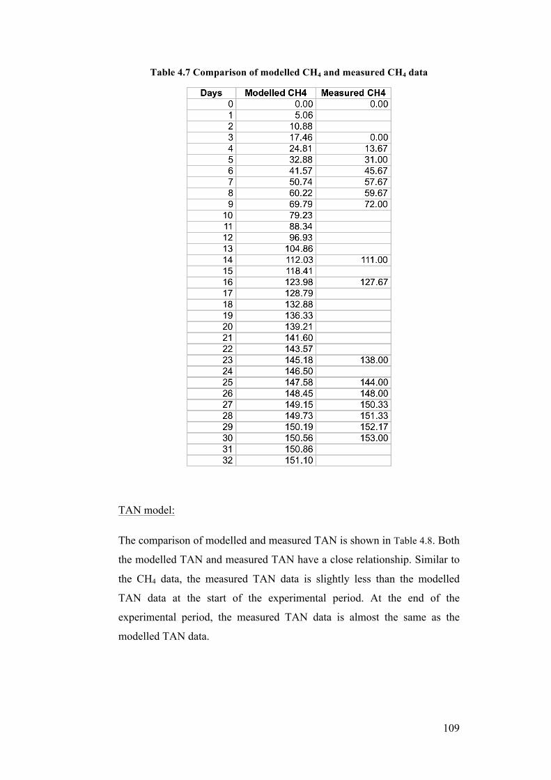
109

Table 4.7 Comparison of modelled CH4 and measured CH4 data

TAN model:

The comparison of modelled and measured TAN is shown in Table 4.8. Both

the modelled TAN and measured TAN have a close relationship. Similar to

the CH4 data, the measured TAN data is slightly less than the modelled

TAN data at the start of the experimental period. At the end of the

experimental period, the measured TAN data is almost the same as the

modelled TAN data.

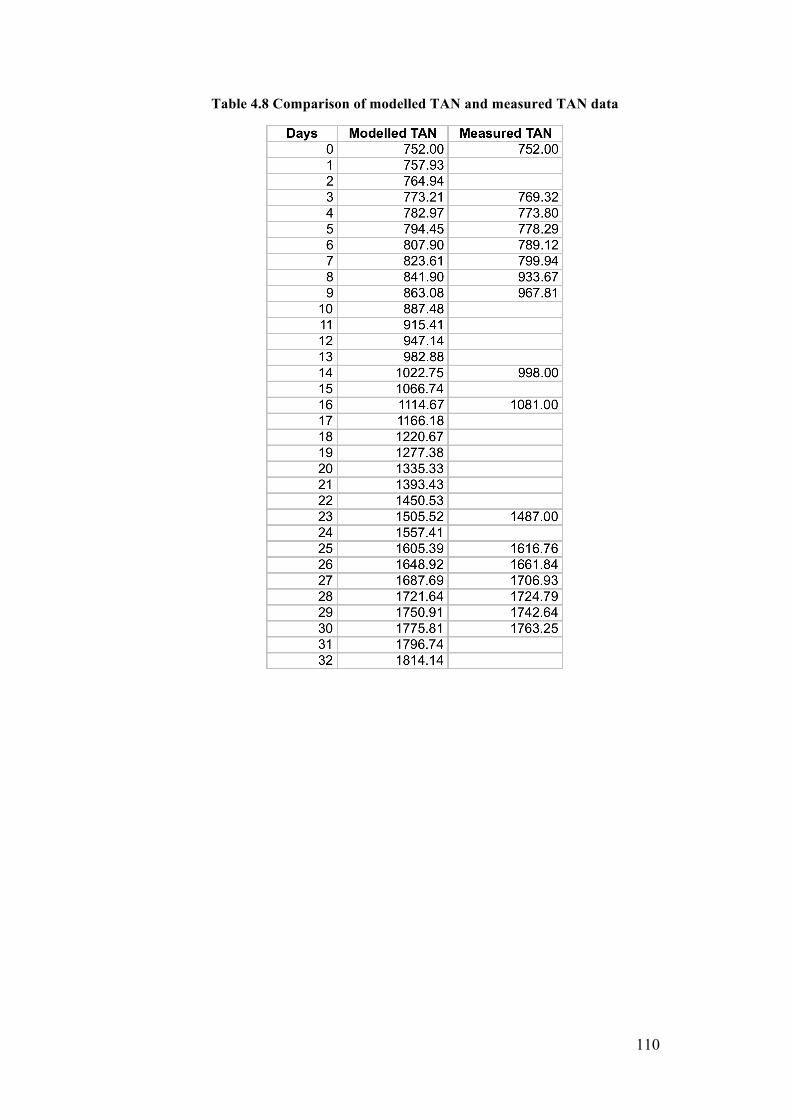
110

Table 4.8 Comparison of modelled TAN and measured TAN data

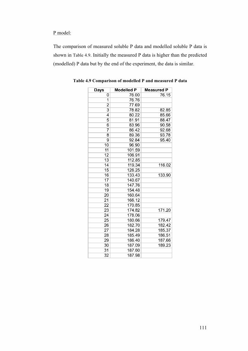
111

P model:

The comparison of measured soluble P data and modelled soluble P data is

shown in Table 4.9. Initially the measured P data is higher than the predicted

(modelled) P data but by the end of the experiment, the data is similar.

Table 4.9 Comparison of modelled P and measured P data

112

4.5 Discussion

The methane model developed in this thesis is markedly different to other

published models (Andrews 1969; Chen and Hashimoto 1978; Hill 1982;

Kleinstreuer and Powegha 1982; Mosey 1983; Moletta, Verrier et al. 1986;

Angelidaki, Ellegaard et al. 1993; Romli 1993; Siegrist, Renggli et al.

1993). These previously published models assume microbial growth as the

limiting step. Microbes grow on substrate and production of biogas in turn is

proportional to the microbial growth on substrates. The initial assumption

that methanogensis was the limiting step in the process appears to be

incorrect. From the results we know that methane production is proportional

to COD reduction. However soluble P and TAN were not proportional to

COD.

The volume of methane obtained was lower than conventional anaerobic

digestion processes. It is known from literature that

1g of COD reduced ~ 0.5 L of CH4 (Chen 1983; (Hill and Barth 1977; Hill

1982)

The average COD reduction in our experimental set up was 7 g. According

to the above equation, approximately 3.5 L of CH4 should be produced but

the average CH4 obtained was approximately 150 mL. This is markedly

lower than the expected value. This could be due to the following reasons.

• One of the reasons for reduced CH4 was leaks in the system.

Considerable volumes of CH4 could have been lost through minute

gaps in the transfer tubes and Schott bottle caps. Approximately 30%

of the methane is estimated to be lost due to leaks in the system.

• Raw piggery effluent obtained from the piggery could have

undergone a significant percentage of anaerobic digestion process

while stored in the piggery sump for 2-3 days before collection.

Therefore only a small part of the COD reduced accounted for the

CH4 production while the remainder must have been transformed

into some other product which we are unaware of at this stage.

113

Further investigation into this was beyond the scope of this PhD

research.

• Presence of other electron acceptors in the system (e.g. oxygen,

sulphate, nitrate, oxidized metals etc) will result in a lower methane

yield because oxidation by bacteria is energetically favoured over

methanogenesis.

The initial lag phase for 3 days during which there was negligible CH4

production could be due to the presence of oxygen in the headspace, which

remained after CO2 was absorbed. The continued production of CH4 even

after 30 days could be due to the fact that some of the less degradable

substances become available as substrates at that time.

A number of differences have been observed in temperature response as

well. Anaerobic digestion microbes normally develop best around human

body temperature (37 0C). Our results indicated that temperature responses

are highest for 45 0C. For CH4, both the growth and death rates peak at

45 0C, growth rate being slightly less than death rate. For soluble P, death

rate peaks at 45 0C, while growth rate is noticeably less than death rate. In

both these cases, the microbes are expiring faster than they are growing. For

TAN death rate peaks at 45 0C, growth rate is almost same as death rate

with growth rate increasing slightly.

4.6 Further Work

This model provides a basis for initiating a mathematical model for the

anaerobic digestion component of the IBS. Further work, listed below,

needs to be done in this area.

• The validity of the model should be checked at different input

concentrations of piggery effluent over a wider range. This could not

be accomplished during this research due to the limited availability

of the pilot scale anaerobic digestion system. It is recommended that

114

the model should be validated against data obtained from the pilot

scale anaerobic digestion system for a period of 2 years at least.

• The model should be applied to the large scale IBS, when it is

constructed.

• The model needs to be validated against different wastes and

effluents. The kinetic constants for these different wastes need to be

determined.

115

5 Modelling Commercial Scale Integrated

Biosystems

5.1 Introduction

A mathematical model was developed for the anaerobic digestion

component of the IBS in Chapter 4. The purpose of the anaerobic digestion

model is to predict the values of total ammonia nitrogen (TAN) and soluble

phosphorus (P) at the end of the anaerobic digestion process of raw piggery

effluent. The values of TAN and P (presented in Chapter 3) form the basis

of input to the dynamic model DYRESM CAEDYM, which is used to

model the aquaculture stages of the IBS which will be discussed in detail in

this chapter.

The aquaculture component of the IBS consists of the bioconversion stages

of phytoplankton, zooplankton and fish. Each stage is able to accept the

input effluent from the previous stage and the nutrient load is effectively

reduced so the wastewater forms an appropriate input to the subsequent

stage. Phytoplankton (microalgae) growth is the first component in the

aquaculture stage of the IBS receiving the anaerobically digested piggery

effluent. The role of the phytoplankton is to utilise the nutrients present in

the wastewater, thereby reducing the percentage of nitrogen and phosphorus

in the piggery effluent. The proposed IBS contains two phytoplankton

ponds. The function of the first pond is to receive the piggery wastewater

which is rich in nutrients (N and P) and initiate a high bioconversion of

algae. The function of the second pond is to further reduce the nutrients in

the wastewater before it is transferred to the zooplankton pond. The second

algal pond, in effect, acts as a buffer so that the nutrient levels in the

wastewater are brought down to a threshold level (< 10 mg/L) acceptable

for the zooplankton to survive. High nutrient level in the wastewater will

cause the zooplankton to die, as they are highly sensitive organisms

(Lampert and Taylor 1985).

116

Zooplankton is the second component in the aquaculture stage of the IBS.

Zooplankton play an important role in water body dynamics, as grazers that

control phytoplankton and bacterial populations, as a food source for higher

trophic levels and in the excretion of dissolved nutrients (Bruce, Hamilton et

al. 2006). Zooplankton grazing on phytoplankton can transfer more than

50% of carbon fixed by algae to higher trophic levels (Scavia 1980).

Zooplankton excretion strongly influences trophic dynamics in ecosystems

by contributing inorganic N and P for primary and bacterial production

(Lehman 1980; Wen and Peters 1994; Gilbert 1998). The factors controlling

zooplankton growth include temperature, zooplankton and phytoplankton

biomass and species composition, internal nutrient ratios and mixing

regimes (Hudson and Taylor 1996; Hudson, Taylor et al. 1999).

In the IBS, the population of zooplankton is critical as this will determine

the bioconversion of algae resulting in reduction of algae and nutrients in

the wastewater. The impact of zooplankton grazing on phytoplankton

biomass and the significance of this impact has been the focus of many

investigations (Hodgkin and Rippingale 1971; Rippingale and Hodgkin

1974a; Rippingale and Hodgkin 1974b; Rippingale and Hodgkin 1977;

Griffiths and Caperon 1979; Stearns, Litaker et al. 1987; Svensson and

Stenson 1991; Cyr and Pace 1992; Rippingale 1994). There has been ample

research conducted on the role of zooplankton in controlling the population

of algae through grazing (Harris 1986; De Melo, France et al. 1992; Boon,

Bunn et al. 1994). There is evidence from past studies that the depletion of

phytoplankton biomass is dependent on the density and size of the

zooplankton grazers (Martin 1970; Gamble 1978; Lampert and Taylor 1985;

Vanni 1987; Turner and Granelli 1992), diurnal variation in zooplankton

feeding rates (McAllister 1971; Mackas and Bohrer 1976; Lampert and

Taylor 1985; Peterson, Painting et al. 1990) and phytoplankton abundance

(Mullin and Brooks 1970; Frost 1972; Reeve and Walter 1977; Ambler

1986; Durbin and Durbin 1992).

Numerous models have previously been used to evaluate different aspects of

zooplankton dynamics in lakes (Scavia 1980; Lunte and Leucke 1990;

117

Krivtsov, Goldspink et al. 2001; Chen, Ji et al. 2002; Hongping and Jianyi

2002; Ji, Chen et al. 2002; Håkanson and Boulion 2003; Rukhovets,

Astrakhantsev et al. 2003; Bruce, Hamilton et al. 2006), reservoirs (Osidele

and Beck 2004; Romero, Antenucci et al. 2004), and estuaries (Griffin,

Herzfeld et al. 2001; Robson and Hamilton 2004). These models range from

simple mass balances to complex simulation tools using a large number of

parameters in hydrodynamic processes (Robson and Hamilton 2004). Some

models provide more detailed information on the spatial and temporal

changes in the nutrients between different trophic levels in a large water

body which is possible with the availability of field or laboratory data.

These models can be used to predict how the fluxes change in response to

the different environmental factors (Bruce, Hamilton et al. 2006)

Fish ponds form the final component in the aquaculture stage of the IBS as

fish are sensitive to nutrient pollution. The function of the fish ponds is to

receive the wastewater from the zooplankton ponds and promote fish

growth by bioconversion of fish utilising the zooplankton and nutrients from

the zooplankton pond, leaving cleaner water which can be reused in the

piggery or other livestock enterprises for flushing or used in other

enterprises like horticulture.

The development of the mathematical model for the aquaculture stage of the

IBS is discussed in detail in the subsequent sections.

5.1.1 Model Description

The dynamic DYRESM CAEDYM model developed at the Centre for

Water Research, University of Western Australia (www.cwr.uwa.edu.au),

which has previously been used for mathematical modelling of water bodies

(Hamilton and Schladow 1997; Bruce, Hamilton et al. 2006; Burger,

Hamilton et al. 2008) was used for this study. DYRESM is a one

dimensional model which resolves around vertical distribution of

temperature, salinity and density in lakes and reservoirs based on a dynamic

Lagrangian structure. It simulates the lake as horizontally uniform layers

that expand and contract in response to heat, mass and momentum

exchanges (Imberger 1981; Gal, Imberger et al. 2003). DYRESM has been

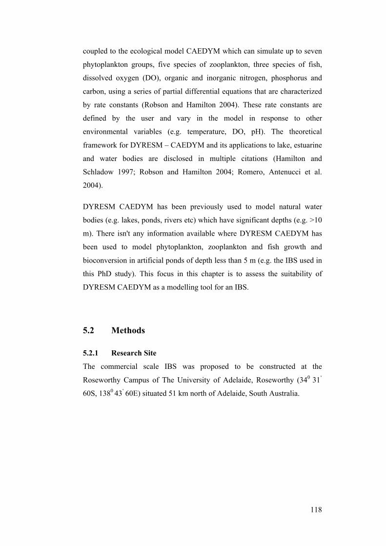
118

coupled to the ecological model CAEDYM which can simulate up to seven

phytoplankton groups, five species of zooplankton, three species of fish,

dissolved oxygen (DO), organic and inorganic nitrogen, phosphorus and

carbon, using a series of partial differential equations that are characterized

by rate constants (Robson and Hamilton 2004). These rate constants are

defined by the user and vary in the model in response to other

environmental variables (e.g. temperature, DO, pH). The theoretical

framework for DYRESM – CAEDYM and its applications to lake, estuarine

and water bodies are disclosed in multiple citations (Hamilton and

Schladow 1997; Robson and Hamilton 2004; Romero, Antenucci et al.

2004).

DYRESM CAEDYM has been previously used to model natural water

bodies (e.g. lakes, ponds, rivers etc) which have significant depths (e.g. >10

m). There isn't any information available where DYRESM CAEDYM has

been used to model phytoplankton, zooplankton and fish growth and

bioconversion in artificial ponds of depth less than 5 m (e.g. the IBS used in

this PhD study). This focus in this chapter is to assess the suitability of

DYRESM CAEDYM as a modelling tool for an IBS.

5.2 Methods

5.2.1 Research Site

The commercial scale IBS was proposed to be constructed at the

Roseworthy Campus of The University of Adelaide, Roseworthy (340 31‘

60S, 1380 43‘ 60E) situated 51 km north of Adelaide, South Australia.

119

Figure 5.1 Schematic of the proposed commercial scale IBS

Experimental data from the pilot scale anaerobic digestion system and

mesocosm aquaculture set up were used as inputs for DYRESM CAEDYM.

These inputs were then used in the model set up for the proposed

commercial scale IBS and it was tested to assess the suitability of DYRESM

CAEDYM as an effective modelling tool for the IBS. The outputs from the

model would then provide guidance for the operational control and

management for the proper functioning of the commercial scale IBS system.

5.2.2 Alterations to the original source code of DYRESM CAEDYM

Application of DYRESM CAEDYM to evaluate aquatic management

strategies have been widely applied to lakes, reservoirs, rivers, estuaries and

coastal zones. These water bodies cover a significant area and have a large

depth. The program for DYRESM CAEDYM is developed in order to

Algae Pond

Zooplankton

Pond

Fish Pond

Anaerobically digested

piggery effluent

Clean

Water

120

succesfully simulate water bodies of depths greater than 5 m. Lake Rotorua,

(area 79 km2, mean depth 10.8 m) is the shallowest water body modelled

using DYRESM CAEDYM reported in literature (Burger, Hamilton et al.

2008).

The ponds proposed to be constructed as part of the IBS had an area of 100

m2 and mean depth 1.0 m. Hence the initial trial simulations crashed as the

model could not successfully run simulations for such a shallow depth.

After discussions with other researchers using the same model, a need to

modify the original source code of DYRESM CAEDYM was identified.

5.2.2.1 Compilation of the source code

During a visit to the Centre for Water Research (CWR), University of

Western Australia (UWA), Perth in November 2007, the source code for the

model was obtained from the UWA researchers. The source code was

compiled and built using Intel Visual FORTRAN 10.1 on Microsoft Visual

Studio 2005 making use of instructions posted on the CWR Model User’s

Forum. The purpose of compilation of the source code was to create an

executable code to run the model. This executable code could be re created

multiple times by altering the source code which would be suitable for

running simulations for the large scale IBS. The new executable code was

evaluated by running the test files to ensure that there was no error in

compilation.

5.2.2.2 Breakpoints

It was observed that the program crashed while executing the subprogram

dyconsts.f90. The dyconsts.f90 file contains parameter constants required to

compile the model simulations successfully.

In the dyconsts.f90 file the following parameters were changed.

• AREA_HT_DELTA_Z: This parameter deals with the z-grid spacing

used for determining the coefficients alpha and beta used to create

piecewise smooth function of area vs. height.

• COEFFS_TBL_DELTA_Z: This parameter deals with the z-grid

spacing used in determining the area height function coefficients.

121

• INTERP_DELTA_Z: This parameter deals with the z-grid spacing used

for interpolating cumulative volumes and layer surface areas.

• MIN_GRID_THICK: This parameter deals with the minimum allowed

grid thickness for surface layer re grid.

These parameters represent the size of the discrete intervals describing the

grid array that relates grid heights to sediment area. Data from the

morphology file and the above mentioned parameters are interpolated

during simulations to produce a finer grid, which can be used in DYRESM

to relate the different layers to a specific sediment area. The formation of

the simulation grid is dependent on the depth of the water body which is to

be simulated. As the depth of the water body is decreased, the value of the

above parameters is also decreased which gives a higher vertical grid

resolution necessary to fit in the shallow depth. This is necessary to run the

simulations successfully.

5.2.3 Input Data

5.2.3.1 Meteorological Data

Meteorological data is one of the key driving forces to run DYRESM

CAEDYM. Daily meteorological data required as input to the DYRESM

CAEDYM model was taken from the Roseworthy Automatic Weather

Station [AWS Bureau of Meteorology Station 023122] situated at the

Roseworthy Campus, The University of Adelaide. Data included short wave

radiation, daily averages of air temperature, total daily rainfall and wind

speed. The closest cloud cover observations were taken at Rosedale, 10 km

to the east. Daily averages of relative humidity (RH) and air temperature

were used to derive the mean daily water vapour pressure input to the model

(Antenucci and Imerito 2002).

The meteorological data input file requires vapour pressure data as one of

the essential input parameters. The meteorological data file obtained from

the Roseworthy AWS had data for relative humidity and air temperature

instead of vapour pressure. Hence vapour pressure was calculated using the

122

formula given in the DYRESM User Science Manual (Imerito 2007). The

details of the equation are given below.

Vapour Pressure Based on Relative Humidity and Air Temperature:

⎥⎥⎦

⎤

⎢⎢⎣

⎡⎟⎟⎠

⎞⎜⎜⎝

⎛+⎟⎟⎠

⎞⎜⎜⎝

⎛

+⎟⎠

⎞⎜⎝

⎛= cbqqahe

D

Da

*303.2exp100

Eq. 5.1 (T.V.A. 1972)

where

• ea = vapour pressure [hPa]

• h = relative humidity of air [%]

• qD = dry bulb air temperature [0C]

and the coefficients for over water calculations are

a = 7.5

b = 237.3

c = 0.7858

Vapour Pressure is one of the inputs in the meteorological file required to

run the DYRESM simulations. Since this data was not available from the

Roseworthy Agricultural Weather Station [AWS Station 023122], the above

formula was used to calculate vapour pressure using relative humidity and

air temperature.

The daily meteorological data collected over a period from 1st June 2006 till

31st May 2007 is presented in Figure 5.2.

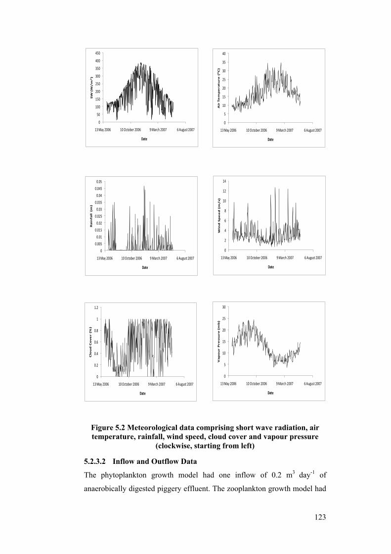
123

Figure 5.2 Meteorological data comprising short wave radiation, air temperature, rainfall, wind speed, cloud cover and vapour pressure

(clockwise, starting from left)

5.2.3.2 Inflow and Outflow Data

The phytoplankton growth model had one inflow of 0.2 m3 day-1 of

anaerobically digested piggery effluent. The zooplankton growth model had

0

50

100

150

200

250

300

350

400

450

13 May 2006 10 October 2006 9 March 2007 6 August 2007

SW (W/m

2)

Date

0

5

10

15

20

25

30

35

40


Air Temperature (0C)

Date

00.0050.010.0150.020.0250.030.0350.040.0450.05


Rainfall (m)

Date

0

2

4

6

8

10

12

14


Wind Speed (m/s)

Date

0

0.2

0.4

0.6

0.8

1

1.2


Cloud Cover (%

)

Date

0

5

10

15

20

25

30


Vapour Pressure (mb)

Date

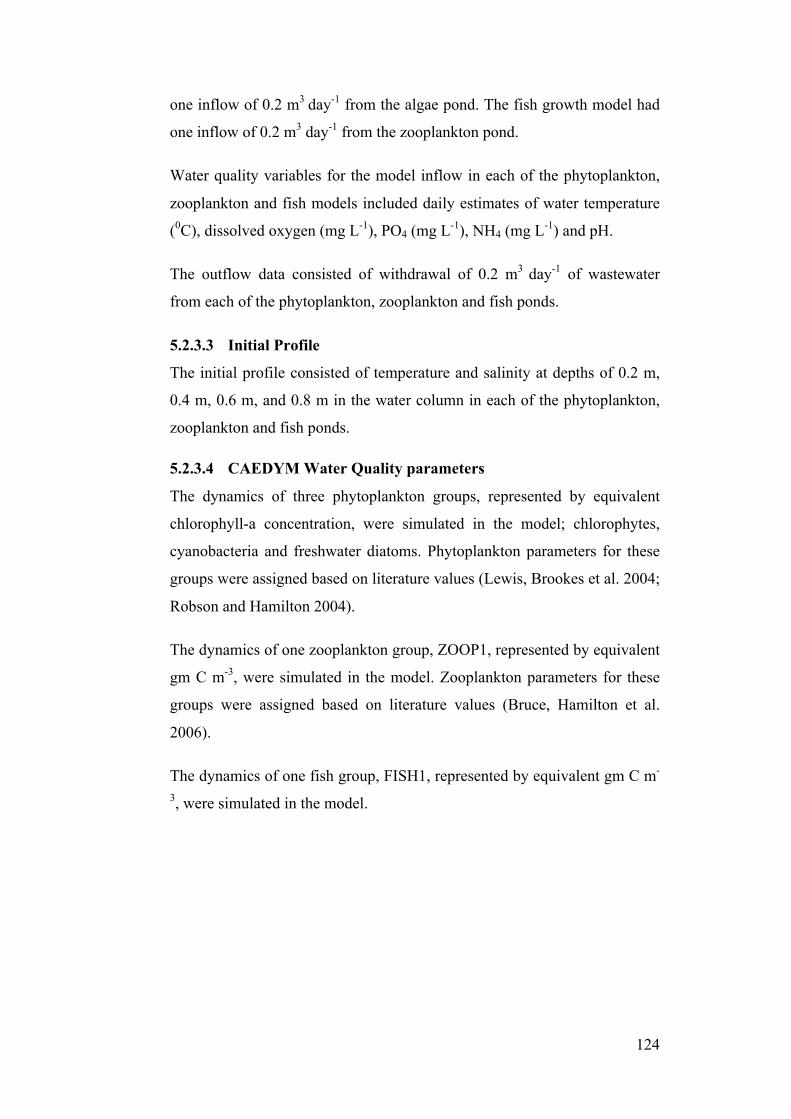
124

one inflow of 0.2 m3 day-1 from the algae pond. The fish growth model had

one inflow of 0.2 m3 day-1 from the zooplankton pond.

Water quality variables for the model inflow in each of the phytoplankton,

zooplankton and fish models included daily estimates of water temperature

(0C), dissolved oxygen (mg L-1), PO4 (mg L-1), NH4 (mg L-1) and pH.

The outflow data consisted of withdrawal of 0.2 m3 day-1 of wastewater

from each of the phytoplankton, zooplankton and fish ponds.

5.2.3.3 Initial Profile

The initial profile consisted of temperature and salinity at depths of 0.2 m,

0.4 m, 0.6 m, and 0.8 m in the water column in each of the phytoplankton,

zooplankton and fish ponds.

5.2.3.4 CAEDYM Water Quality parameters

The dynamics of three phytoplankton groups, represented by equivalent

chlorophyll-a concentration, were simulated in the model; chlorophytes,

cyanobacteria and freshwater diatoms. Phytoplankton parameters for these

groups were assigned based on literature values (Lewis, Brookes et al. 2004;

Robson and Hamilton 2004).

The dynamics of one zooplankton group, ZOOP1, represented by equivalent

gm C m-3, were simulated in the model. Zooplankton parameters for these

groups were assigned based on literature values (Bruce, Hamilton et al.

2006).

The dynamics of one fish group, FISH1, represented by equivalent gm C m-

3, were simulated in the model.

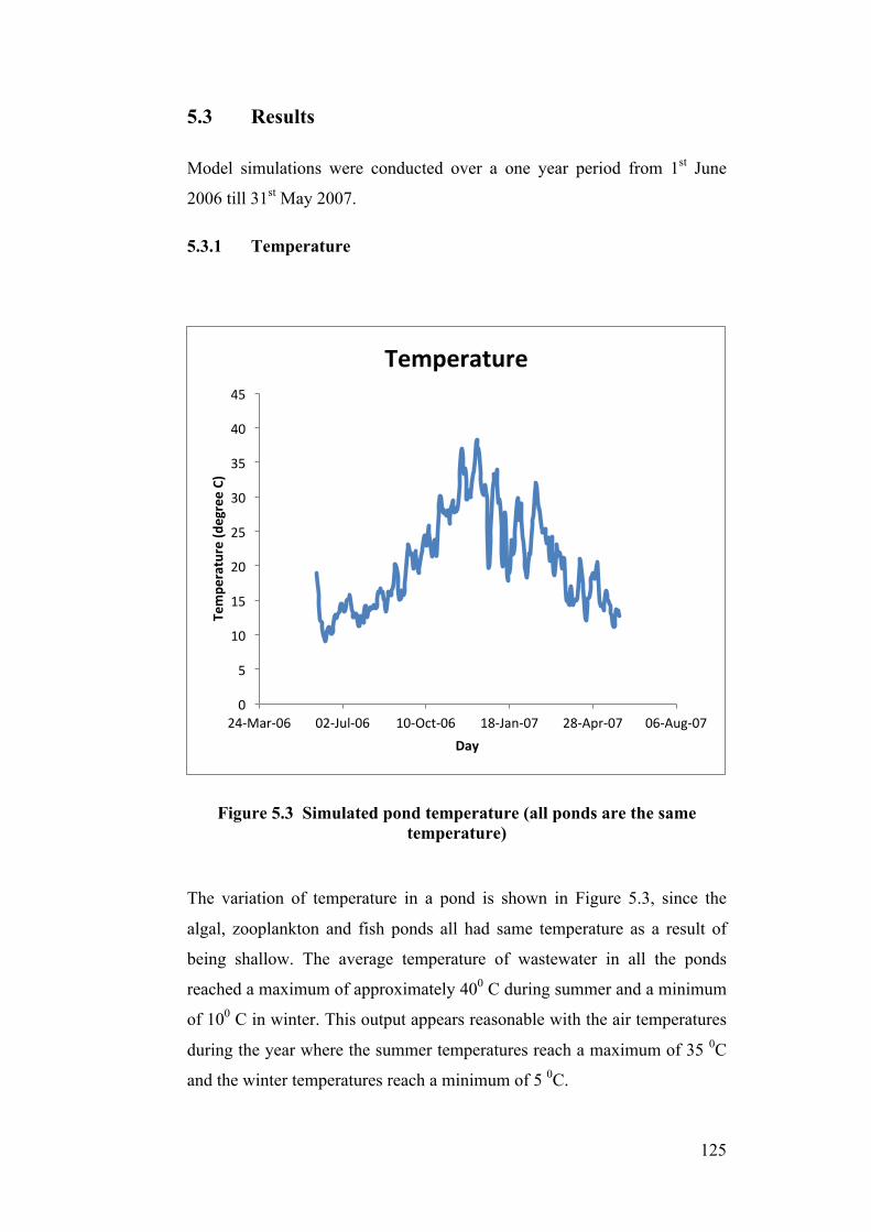
125

5.3 Results

Model simulations were conducted over a one year period from 1st June

2006 till 31st May 2007.

5.3.1 Temperature

Figure 5.3 Simulated pond temperature (all ponds are the same temperature)

The variation of temperature in a pond is shown in Figure 5.3, since the

algal, zooplankton and fish ponds all had same temperature as a result of

being shallow. The average temperature of wastewater in all the ponds

reached a maximum of approximately 400 C during summer and a minimum

of 100 C in winter. This output appears reasonable with the air temperatures

during the year where the summer temperatures reach a maximum of 35 0C

and the winter temperatures reach a minimum of 5 0C.

0

5

10

15

20

25

30

35

40

45

24-‐Mar-‐06 02-‐Jul-‐06 10-‐Oct-‐06 18-‐Jan-‐07 28-‐Apr-‐07 06-‐Aug-‐07

Tempe

rature (d

egree C)

Day

Temperature

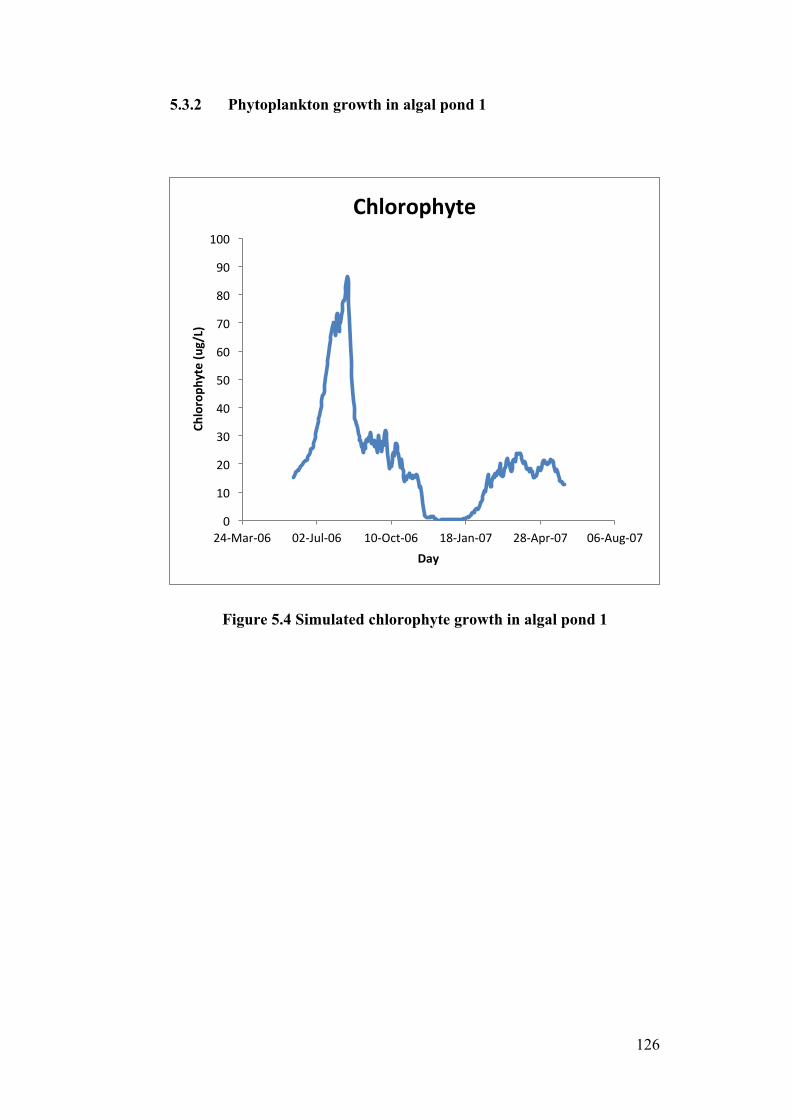
126

5.3.2 Phytoplankton growth in algal pond 1

Figure 5.4 Simulated chlorophyte growth in algal pond 1

0

10

20

30

40

50

60

70

80

90

100


Chloroph

yte (ug/L)

Day

Chlorophyte

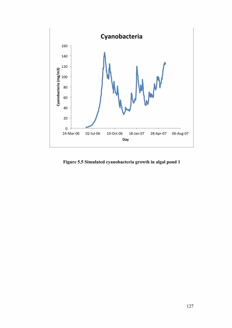
127

Figure 5.5 Simulated cyanobacteria growth in algal pond 1

0

20

40

60

80

100

120

140

160


Cyan

obacteria

(mg/m3)

Day

Cyanobacteria

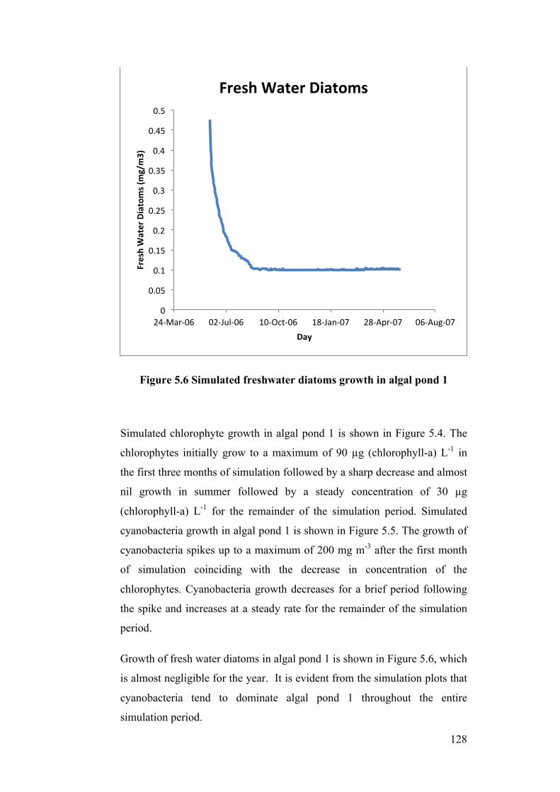
128

Figure 5.6 Simulated freshwater diatoms growth in algal pond 1

Simulated chlorophyte growth in algal pond 1 is shown in Figure 5.4. The

chlorophytes initially grow to a maximum of 90 µg (chlorophyll-a) L-1 in

the first three months of simulation followed by a sharp decrease and almost

nil growth in summer followed by a steady concentration of 30 µg

(chlorophyll-a) L-1 for the remainder of the simulation period. Simulated

cyanobacteria growth in algal pond 1 is shown in Figure 5.5. The growth of

cyanobacteria spikes up to a maximum of 200 mg m-3 after the first month

of simulation coinciding with the decrease in concentration of the

chlorophytes. Cyanobacteria growth decreases for a brief period following

the spike and increases at a steady rate for the remainder of the simulation

period.

Growth of fresh water diatoms in algal pond 1 is shown in Figure 5.6, which

is almost negligible for the year. It is evident from the simulation plots that

cyanobacteria tend to dominate algal pond 1 throughout the entire

simulation period.

0

0.05

0.1

0.15

0.2

0.25

0.3

0.35

0.4

0.45

0.5


Fresh Water Diatoms (mg/m3)

Day

Fresh Water Diatoms

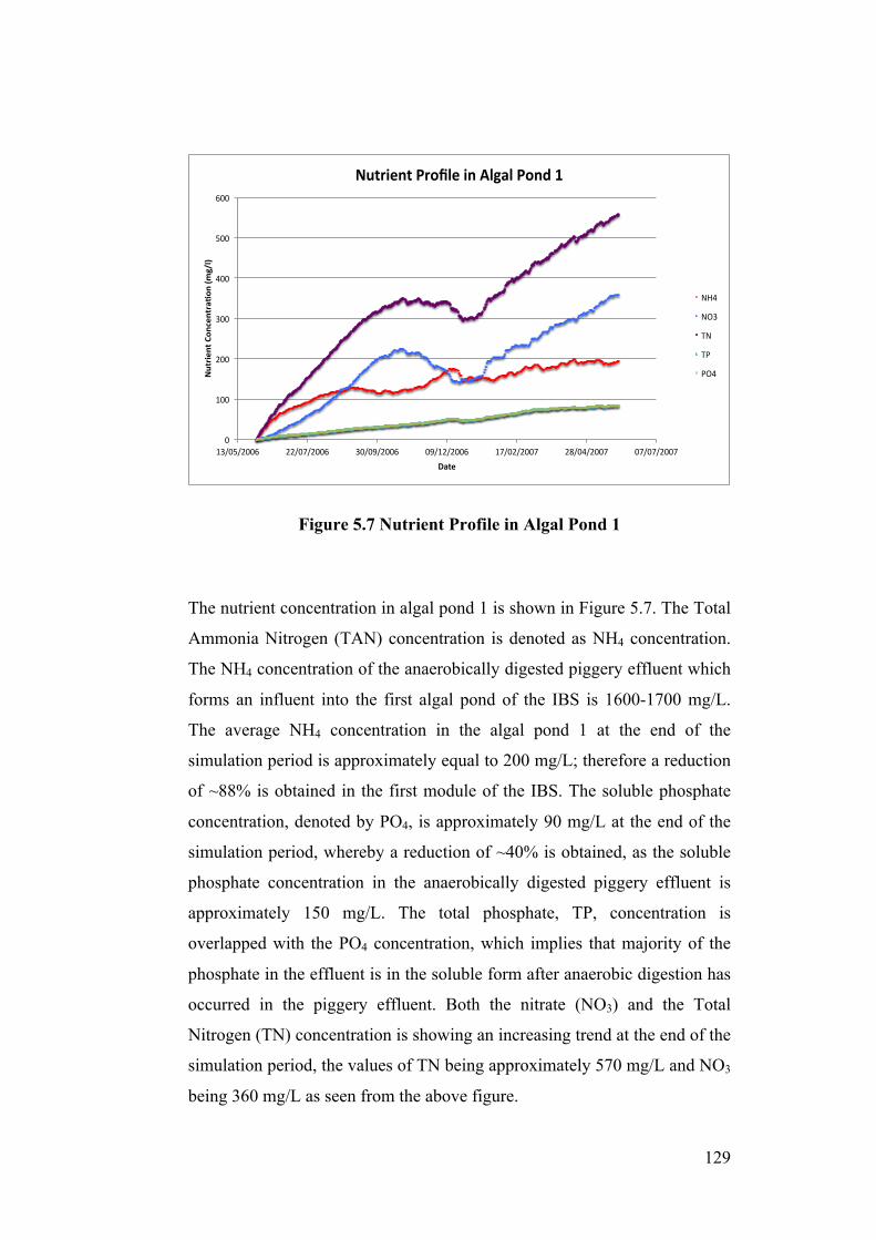
129

Figure 5.7 Nutrient Profile in Algal Pond 1

The nutrient concentration in algal pond 1 is shown in Figure 5.7. The Total

Ammonia Nitrogen (TAN) concentration is denoted as NH4 concentration.

The NH4 concentration of the anaerobically digested piggery effluent which

forms an influent into the first algal pond of the IBS is 1600-1700 mg/L.

The average NH4 concentration in the algal pond 1 at the end of the

simulation period is approximately equal to 200 mg/L; therefore a reduction

of ~88% is obtained in the first module of the IBS. The soluble phosphate

concentration, denoted by PO4, is approximately 90 mg/L at the end of the

simulation period, whereby a reduction of ~40% is obtained, as the soluble

phosphate concentration in the anaerobically digested piggery effluent is

approximately 150 mg/L. The total phosphate, TP, concentration is

overlapped with the PO4 concentration, which implies that majority of the

phosphate in the effluent is in the soluble form after anaerobic digestion has

occurred in the piggery effluent. Both the nitrate (NO3) and the Total

Nitrogen (TN) concentration is showing an increasing trend at the end of the

simulation period, the values of TN being approximately 570 mg/L and NO3

being 360 mg/L as seen from the above figure.

0"

100"

200"

300"

400"

500"

600"

13/05/2006" 22/07/2006" 30/09/2006" 09/12/2006" 17/02/2007" 28/04/2007" 07/07/2007"

Nutrie

nt(Con

centra-o

n((m

g/l)(

Date(

Nutrient(Profile(in(Algal(Pond(1(

NH4"

NO3"

TN"

TP"

PO4"

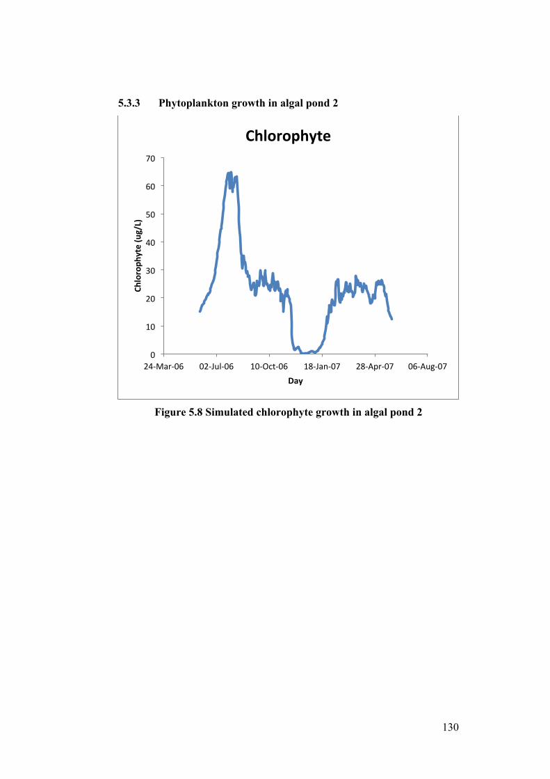
130

5.3.3 Phytoplankton growth in algal pond 2

Figure 5.8 Simulated chlorophyte growth in algal pond 2

0

10

20

30

40

50

60

70


Chloroph

yte (ug/L)

Day

Chlorophyte

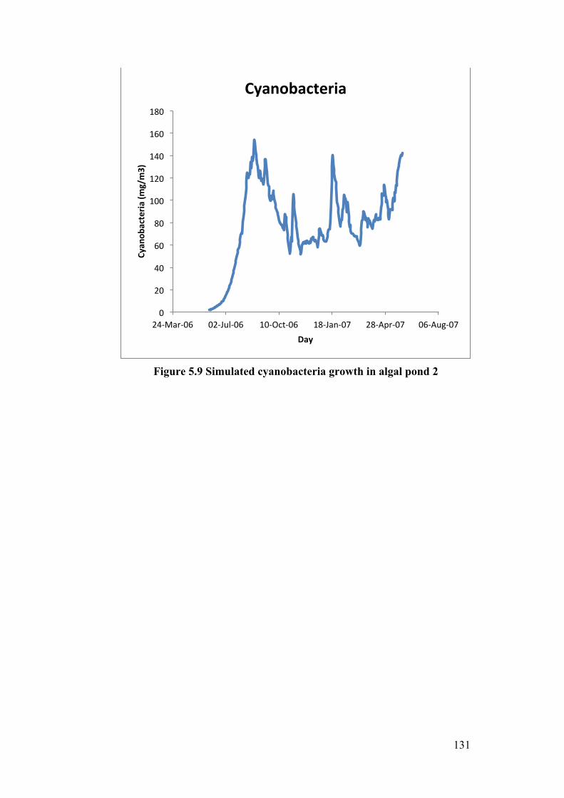
131

Figure 5.9 Simulated cyanobacteria growth in algal pond 2

0

20

40

60

80

100

120

140

160

180


Cyan

obacteria

(mg/m3)

Day

Cyanobacteria

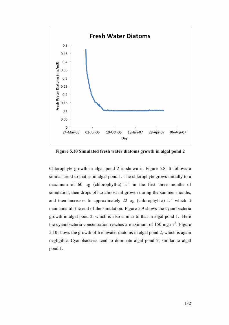
132

Figure 5.10 Simulated fresh water diatoms growth in algal pond 2

Chlorophyte growth in algal pond 2 is shown in Figure 5.8. It follows a

similar trend to that as in algal pond 1. The chlorophyte grows initially to a

maximum of 60 µg (chlorophyll-a) L-1 in the first three months of

simulation, then drops off to almost nil growth during the summer months,

and then increases to approximately 22 µg (chlorophyll-a) L-1 which it

maintains till the end of the simulation. Figure 5.9 shows the cyanobacteria

growth in algal pond 2, which is also similar to that in algal pond 1. Here

the cyanobacteria concentration reaches a maximum of 150 mg m-3. Figure

5.10 shows the growth of freshwater diatoms in algal pond 2, which is again

negligible. Cyanobacteria tend to dominate algal pond 2, similar to algal

pond 1.

0

0.05

0.1

0.15

0.2

0.25

0.3

0.35

0.4

0.45

0.5


Fresh Water Diatoms (mg/m3)

Day

Fresh Water Diatoms

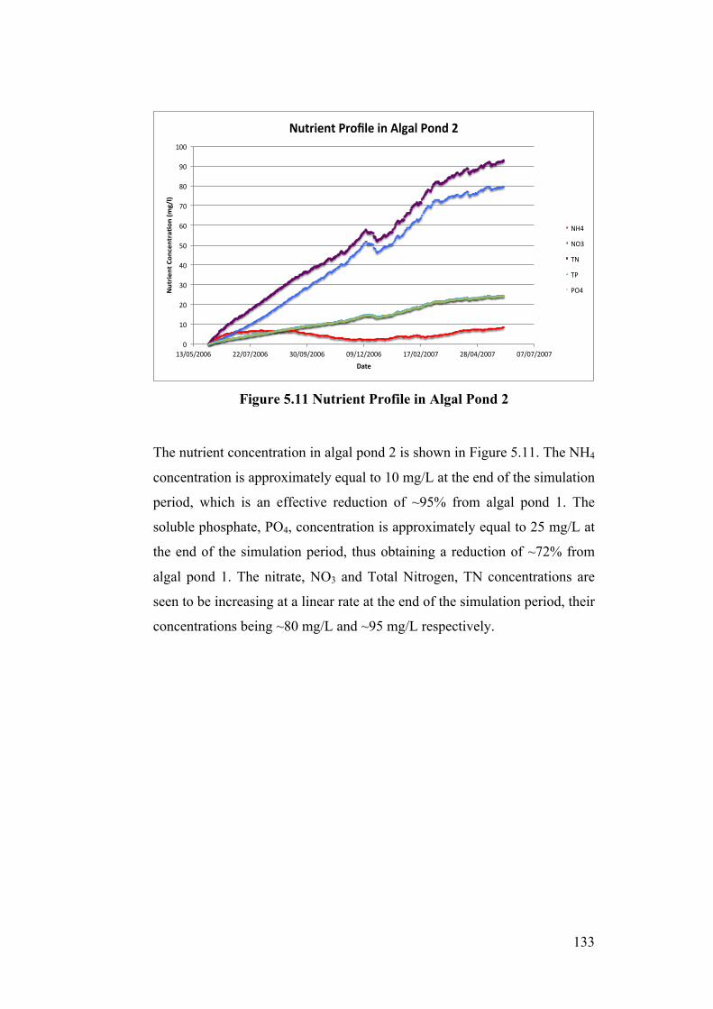
133

Figure 5.11 Nutrient Profile in Algal Pond 2

The nutrient concentration in algal pond 2 is shown in Figure 5.11. The NH4

concentration is approximately equal to 10 mg/L at the end of the simulation

period, which is an effective reduction of ~95% from algal pond 1. The

soluble phosphate, PO4, concentration is approximately equal to 25 mg/L at

the end of the simulation period, thus obtaining a reduction of ~72% from

algal pond 1. The nitrate, NO3 and Total Nitrogen, TN concentrations are

seen to be increasing at a linear rate at the end of the simulation period, their

concentrations being ~80 mg/L and ~95 mg/L respectively.

0"

10"

20"

30"

40"

50"

60"

70"

80"

90"

100"

13/05/2006" 22/07/2006" 30/09/2006" 09/12/2006" 17/02/2007" 28/04/2007" 07/07/2007"

Nutrie

nt(Con

centra-o

n((m

g/l)(

Date(

Nutrient(Profile(in(Algal(Pond(2(

NH4"

NO3"

TN"

TP"

PO4"

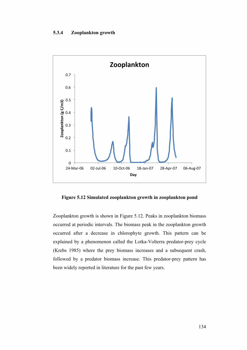
134

5.3.4 Zooplankton growth

Figure 5.12 Simulated zooplankton growth in zooplankton pond

Zooplankton growth is shown in Figure 5.12. Peaks in zooplankton biomass

occurred at periodic intervals. The biomass peak in the zooplankton growth

occurred after a decrease in chlorophyte growth. This pattern can be

explained by a phenomenon called the Lotka-Volterra predator-prey cycle

(Krebs 1985) where the prey biomass increases and a subsequent crash,

followed by a predator biomass increase. This predator-prey pattern has

been widely reported in literature for the past few years.

0

0.1

0.2

0.3

0.4

0.5

0.6

0.7


Zoop

lank

ton (g C/m

3)

Day

Zooplankton

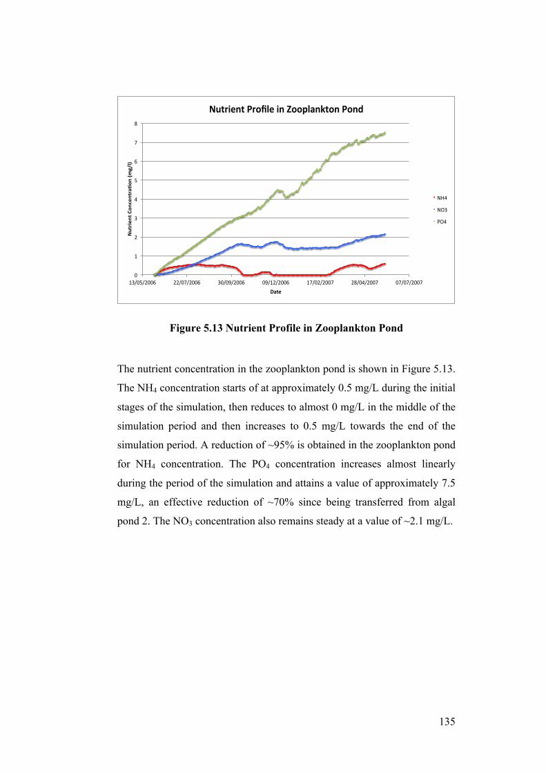
135

Figure 5.13 Nutrient Profile in Zooplankton Pond

The nutrient concentration in the zooplankton pond is shown in Figure 5.13.

The NH4 concentration starts of at approximately 0.5 mg/L during the initial

stages of the simulation, then reduces to almost 0 mg/L in the middle of the

simulation period and then increases to 0.5 mg/L towards the end of the

simulation period. A reduction of ~95% is obtained in the zooplankton pond

for NH4 concentration. The PO4 concentration increases almost linearly

during the period of the simulation and attains a value of approximately 7.5

mg/L, an effective reduction of ~70% since being transferred from algal

pond 2. The NO3 concentration also remains steady at a value of ~2.1 mg/L.

0"

1"

2"

3"

4"

5"

6"

7"

8"

13/05/2006" 22/07/2006" 30/09/2006" 09/12/2006" 17/02/2007" 28/04/2007" 07/07/2007"

Nutrie

nt(Con

centra-o

n((m

g/l)(

Date(

Nutrient(Profile(in(Zooplankton(Pond(

NH4"

NO3"

PO4"

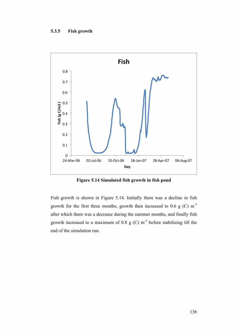
136

5.3.5 Fish growth

Figure 5.14 Simulated fish growth in fish pond

Fish growth is shown in Figure 5.14. Initially there was a decline in fish

growth for the first three months; growth then increased to 0.6 g (C) m-3

after which there was a decrease during the summer months, and finally fish

growth increased to a maximum of 0.8 g (C) m-3 before stabilizing till the

end of the simulation run.

0

0.1

0.2

0.3

0.4

0.5

0.6

0.7

0.8


Fish (g C/m

3 )

Day

Fish

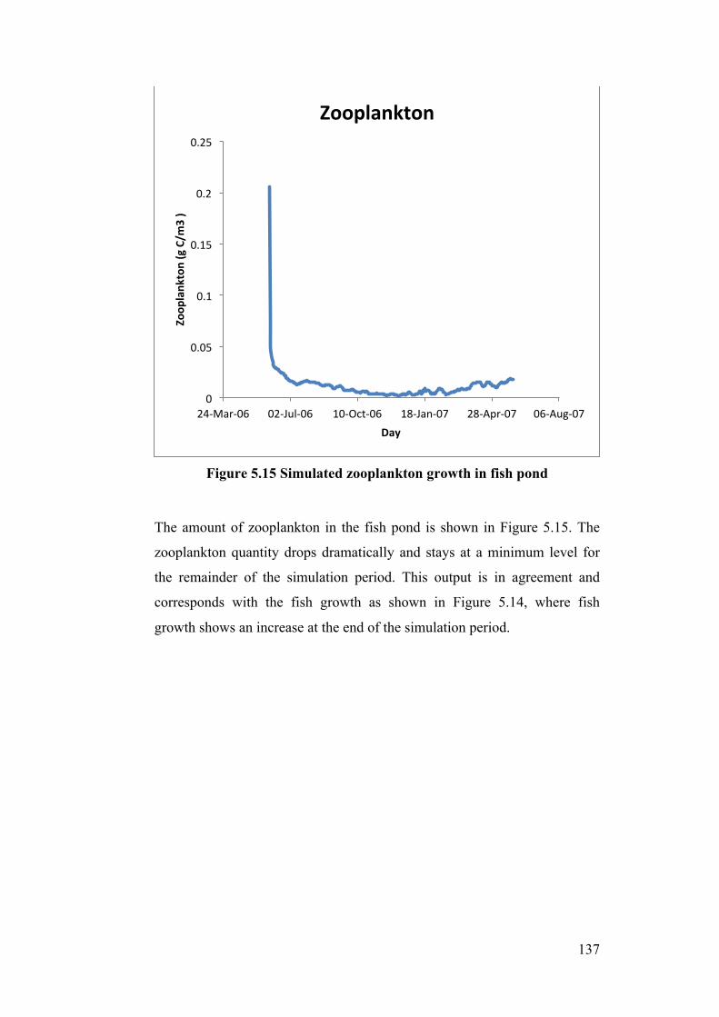
137

Figure 5.15 Simulated zooplankton growth in fish pond

The amount of zooplankton in the fish pond is shown in Figure 5.15. The

zooplankton quantity drops dramatically and stays at a minimum level for

the remainder of the simulation period. This output is in agreement and

corresponds with the fish growth as shown in Figure 5.14, where fish

growth shows an increase at the end of the simulation period.

0

0.05

0.1

0.15

0.2

0.25


Zoop

lank

ton (g C/m

3 )

Day

Zooplankton

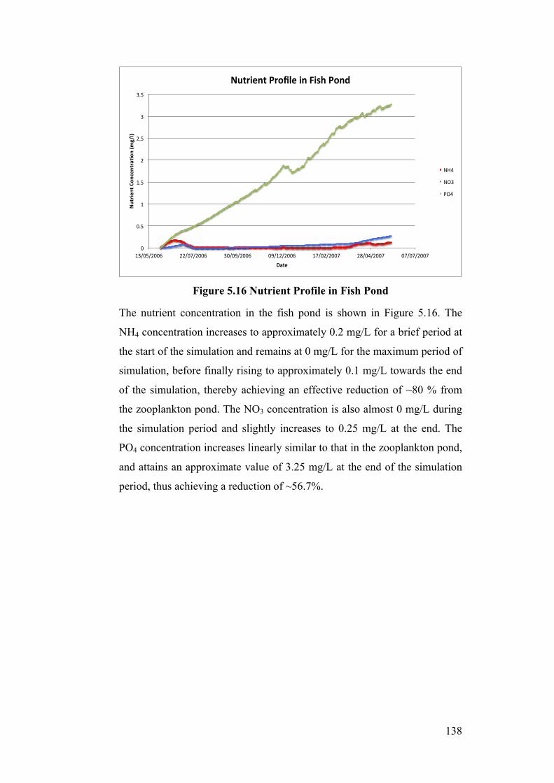
138

Figure 5.16 Nutrient Profile in Fish Pond

The nutrient concentration in the fish pond is shown in Figure 5.16. The

NH4 concentration increases to approximately 0.2 mg/L for a brief period at

the start of the simulation and remains at 0 mg/L for the maximum period of

simulation, before finally rising to approximately 0.1 mg/L towards the end

of the simulation, thereby achieving an effective reduction of ~80 % from

the zooplankton pond. The NO3 concentration is also almost 0 mg/L during

the simulation period and slightly increases to 0.25 mg/L at the end. The

PO4 concentration increases linearly similar to that in the zooplankton pond,

and attains an approximate value of 3.25 mg/L at the end of the simulation

period, thus achieving a reduction of ~56.7%.

0"

0.5"

1"

1.5"

2"

2.5"

3"

3.5"

13/05/2006" 22/07/2006" 30/09/2006" 09/12/2006" 17/02/2007" 28/04/2007" 07/07/2007"

Nutrie

nt(Con

centra-o

n((m

g/l)(

Date(

Nutrient(Profile(in(Fish(Pond(

NH4"

NO3"

PO4"

139

5.4 Discussion

The hydrodynamic and ecological modelling software DYRESM CAEDYM

has been extensively applied to model phytoplankton, zooplankton and fish

growth in water bodies having large depths and surface areas especially

reservoirs, lakes, estuaries and ponds. This study reported in Chapter 5 has

applied the model to simulate phytoplankton, zooplankton and fish growth

in artificially made shallow ponds with a mean depth of 1.0 m. The

parameters used in the source code of the model were altered to successfully

run the model for the IBS ponds. This is a significant achievement in

modelling water bodies of depth <5 m using DYRESM CAEDYM which

has not been done before. The simulated data obtained from this modelling

exercise is based on data obtained from pilot scale and mesocosm

experiments. The model does not incorporate any control management

measures. However the results obtained from this modelling study would

help us in deciding the required management and control measures which

need to be incorporated in order to obtain favourable results.

The phytoplankton, zooplankton and fish growth was simulated using

weather data for the period 1st June 2006 to 31st May 2007. A year’s worth

of meteorological data was used to obtain credible model outputs. The pilot

scale and mesocosm experiments were conducted in extremely temperature

controlled environments. The meterological data provided seasonal

variation input into the model for simulating the IBS which is exposed to

ambient conditions.

The growth of chlorophyte (Chlorella) occurred during the start of the

simulation period in June 2006 but declined as the simulation period

progressed. Chlorophytes reached a maximum concentration of 90 µg (chl-

a) L-1 and 60 µg (chl-a) L-1 in the first and second algal ponds respectively.

The decrease in chlorophyte growth is dominated by cyanobacteria. During

the summer period, there is practically negligible growth of chlorophytes.

The growth of cyanobacteria (Anabaena circinalis) occurs during periods

when there is permanent stratification, which normally does not occur in

140

commercial IBS with effective management and control measures in place.

It is evident from Figure 5.5 that the growth of cyanobacteria occurs during

late spring and summer when there is high insolation. The cyanobacteria

concentration reaches a maximum of 200 mg m-3 and 150 mg m-3 in the first

and second algal ponds respectively. The cyanobacteria concentration

remains constant for the rest of the simulation period.

Cyanobacteria have a higher affinity for nitrogen and phosphorus than other

photosynthetic organisms and can fix atmospheric nitrogen (Boon, Bunn et

al. 1994; Bergman, Gallon et al. 1997; Mur, Skulberg et al. 1999; Ute 2003;

Fiore, Neilan et al. 2005; Hense and Beckmann 2006; Marino and Howarth

2009; Hense and Burchard 2010; Jonathan P 2011; Paerl, Xu et al. 2011).

Cyanobacteria have a growth rate less than that of green algae; however, at

very low light intensities their growth rate is higher. When the turbidity of

the water body is high or at low CO2/ high pH, they have a better chance of

out-competing other species in the water environment, especially when the

concentrations of nitrogen and phosphorus is limited (Mur, Skulberg et al.

1999). Cyanobacteria synthesise and secrete large quantities of

polysaccharides from their cells. This protective coating enables them to

withstand stress brought about by lack of water and high temperatures.

Available phosphorus appears to be a critical factor to stimulate rapid

growth of cyanobacteria during the summer months. Cyanobacteria often

exploit a combination of these features to dominate the water body

(Kardinaal and Visser 2005). Cyanobacterial blooms can flood the water

environment with the biotoxins which they produce. These toxins modify

zooplankton communities and interfere with the development of fish.

Freshwater diatom growth in the IBS ponds was almost negligible. In open

water bodies, the condition that causes the diatom blooms to end is a lack of

silicon. Unlike other nutrients, this is the only major requirement of diatoms

so it is not regenerated in the plankton ecosystem as efficiently as nitrogen

or phosphorus. As the nutrients (N and P) decline along gradients, silicon is

usually the first to be diminished (followed by N and P) (Egge and Aksnes

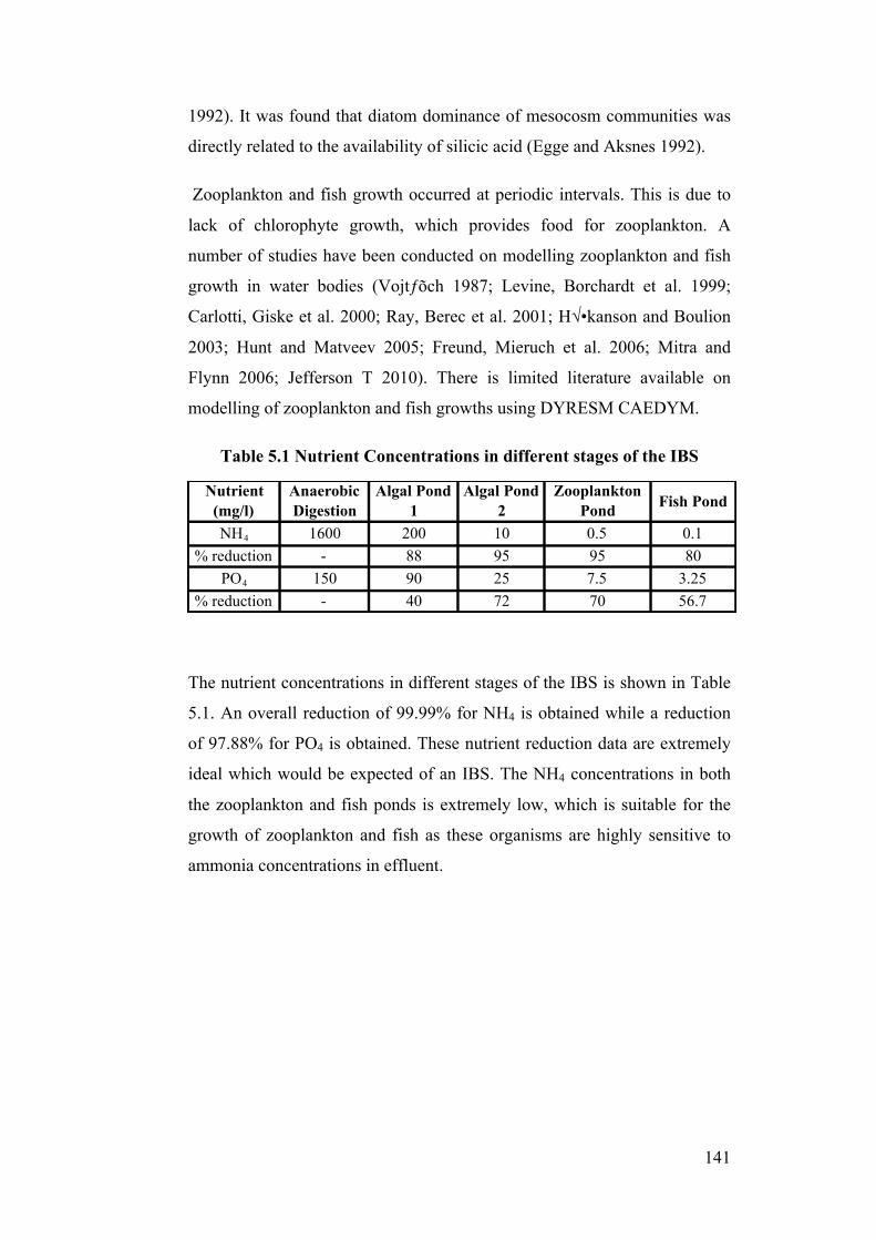
141

1992). It was found that diatom dominance of mesocosm communities was

directly related to the availability of silicic acid (Egge and Aksnes 1992).

Zooplankton and fish growth occurred at periodic intervals. This is due to

lack of chlorophyte growth, which provides food for zooplankton. A

number of studies have been conducted on modelling zooplankton and fish

growth in water bodies (Vojtƒõch 1987; Levine, Borchardt et al. 1999;

Carlotti, Giske et al. 2000; Ray, Berec et al. 2001; H√•kanson and Boulion

2003; Hunt and Matveev 2005; Freund, Mieruch et al. 2006; Mitra and

Flynn 2006; Jefferson T 2010). There is limited literature available on

modelling of zooplankton and fish growths using DYRESM CAEDYM.

Table 5.1 Nutrient Concentrations in different stages of the IBS

The nutrient concentrations in different stages of the IBS is shown in Table

5.1. An overall reduction of 99.99% for NH4 is obtained while a reduction

of 97.88% for PO4 is obtained. These nutrient reduction data are extremely

ideal which would be expected of an IBS. The NH4 concentrations in both

the zooplankton and fish ponds is extremely low, which is suitable for the

growth of zooplankton and fish as these organisms are highly sensitive to

ammonia concentrations in effluent.

Nutrient (mg/l)

Anaerobic Digestion

Algal Pond 1

Algal Pond 2

Zooplankton Pond Fish Pond

NH4 1600 200 10 0.5 0.1% reduction - 88 95 95 80

PO4 150 90 25 7.5 3.25% reduction - 40 72 70 56.7

142

5.4.1 Limitations of the model

The model developed for the aquaculture component of the IBS has certain

limitations.

• The IBS model developed is hypothetical. The commercial scale IBS

could not be constructed at the time this PhD study was conducted.

As a result, the data for validating the model was not available to the

researcher. This proved to be a considerable set back in determining

the validity of the model.

• Parameters which could account for effective management and

control of the IBS has not been accounted for in this model as this

model has used inputs based on experiments conducted in the pilot

and mesocosm stages.

• DYRESM CAEDYM requires both inflow and outflow volumes for

the model to run successfully. The values of inflow and outflow

need to be manually set by the user. However in real life modelling

situations, it is desirable for the user to input only the inflow volume

and a desired depth of the ponds. The outflow volume, water quality

parameters and the bioconversion rates should be automatically

calculated using the input values. Also this model accounts for

controlling the input and output volumes initially by manual

adjustments which is a tedious task.

• DYRESM CAEDYM is primarily designed to model reservoirs,

lakes and water bodies having depths greater than 5m. In order to

model ponds with depths lesser than that, like that in the IBS, the

source code of the model needs to be altered to make it suitable for

the simulations. This is a tedious task and the person needs to have

sufficient programming skills to compile the source code to be able

to run the simulations. As there was only elementary computer

programming skills present at the time of this study, this research

mainly focussed on testing the suitability of this modelling package

for a commercial scale IBS and ways by which it could be modified

to effectively manage and control the IBS.

143

5.4.2 Comparison with algal data obtained from Bolivar Wastewater

Treatment Plant

Bolivar Wastewater Treatment Plant (WWTP) is one of Adelaide’s major

wastewater treatment plants, situated (Latitude: 34º 41' 28.21" S; Longitude:

138º 35' 12.67" E) 26.7 kms north of Adelaide. The treatment plant

processes on average 135 million litres of household and industrial

wastewater every day. The plant has the capacity to handle the wastewater

treatment needs of 1.3 million people. The wastewater passes through

primary screening, primary clarifier, activated sludge treatment, secondary

clarifier, maturation lagoons, and a final filtration unit. Primary effluent is

pumped to a new activated sludge process for secondary treatment. The

activated sludge treatment is known as a suspended growth biological

treatment process because active microorganisms are maintained in

suspension in the wastewater. Treated wastewater or effluent is decanted

from the surface of the settling clarifier tank and then flows by gravity to

stabilisation lagoons. The six-stabilisation lagoons cover a total area of 347

hectares, providing a nominal detention time of about 30 days, for further

treatment by microorganisms, including algae. The lagoons are

approximately 1.2 m deep. These maturation lagoons are significantly

different in size and the water retention time also differs accordingly. The

lagoon/s, which receive the wastewater directly from clarifiers, have the

highest level of nutrients. The conditioning of effluent includes symbiotic

activity by various micro-organisms. This enables continued nitrification

and de-nitrification in the effluent water, growth of algae and establishment

of an eco-system within the stabilisation lagoons. The maturation lagoons

receive wastewater containing an average ammonia concentration of 5-7

mg/l. During winter period ammonia levels will be about 9 mg/l. The

available information indicates no heavy metal content is present in the

wastewater. A significant proportion of the final effluent from the lagoons is

pumped to the Dissolved Air Floatation and Filtration (DAFF) plant to meet

the irrigation needs of market garden crops in the Virginia area through a

pipe line (Virginia Pipeline Scheme).

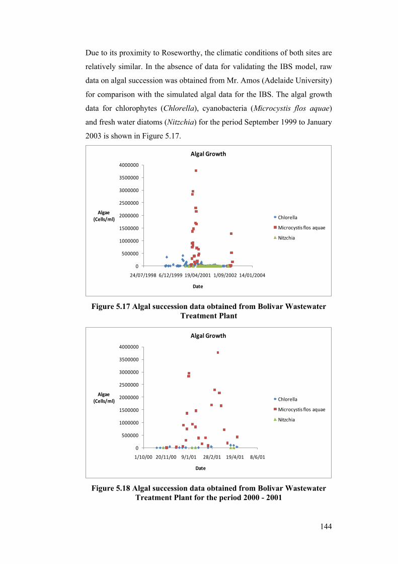
144

Due to its proximity to Roseworthy, the climatic conditions of both sites are

relatively similar. In the absence of data for validating the IBS model, raw

data on algal succession was obtained from Mr. Amos (Adelaide University)

for comparison with the simulated algal data for the IBS. The algal growth

data for chlorophytes (Chlorella), cyanobacteria (Microcystis flos aquae)

and fresh water diatoms (Nitzchia) for the period September 1999 to January

2003 is shown in Figure 5.17.


Treatment Plant


Treatment Plant for the period 2000 - 2001

0

500000

1000000

1500000

2000000

2500000

3000000

3500000

4000000

24/07/1998 6/12/1999 19/04/2001 1/09/2002 14/01/2004

Algae(Cells/ml)

Date

Algal Growth

Chlorella

Microcystis flos aquae

Nitzchia

0

500000

1000000

1500000

2000000

2500000

3000000

3500000

4000000

1/10/00 20/11/00 9/1/01 28/2/01 19/4/01 8/6/01

Algae(Cells/ml)

Date

Algal Growth

Chlorella

Microcystis flos aquae

Nitzchia

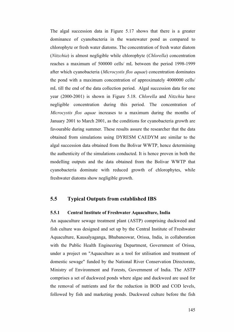
145

The algal succession data in Figure 5.17 shows that there is a greater

dominance of cyanobacteria in the wastewater pond as compared to

chlorophyte or fresh water diatoms. The concentration of fresh water diatom

(Nitzchia) is almost negligible while chlorophyte (Chlorella) concentration

reaches a maximum of 500000 cells/ mL between the period 1998-1999

after which cyanobacteria (Microcystis flos aquae) concentration dominates

the pond with a maximum concentration of approximately 4000000 cells/

mL till the end of the data collection period. Algal succession data for one

year (2000-2001) is shown in Figure 5.18. Chlorella and Nitzchia have

negligible concentration during this period. The concentration of

Microcystis flos aquae increases to a maximum during the months of

January 2001 to March 2001, as the conditions for cyanobacteria growth are

favourable during summer. These results assure the researcher that the data

obtained from simulations using DYRESM CAEDYM are similar to the

algal succession data obtained from the Bolivar WWTP, hence determining

the authenticity of the simulations conducted. It is hence proven in both the

modelling outputs and the data obtained from the Bolivar WWTP that

cyanobacteria dominate with reduced growth of chlorophytes, while

freshwater diatoms show negligible growth.

5.5 Typical Outputs from established IBS

5.5.1 Central Institute of Freshwater Aquaculture, India

An aquaculture sewage treatment plant (ASTP) comprising duckweed and

fish culture was designed and set up by the Central Institute of Freshwater

Aquaculture, Kausalyaganga, Bhubaneswar, Orissa, India, in collaboration

with the Public Health Engineering Department, Government of Orissa,

under a project on "Aquaculture as a tool for utilisation and treatment of

domestic sewage" funded by the National River Conservation Directorate,

Ministry of Environment and Forests, Government of India. The ASTP

comprises a set of duckweed ponds where algae and duckweed are used for

the removal of nutrients and for the reduction in BOD and COD levels,

followed by fish and marketing ponds. Duckweed culture before the fish

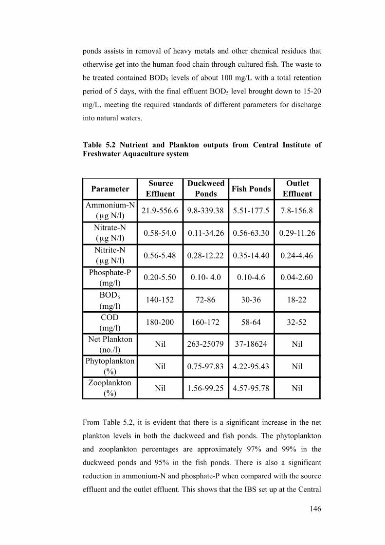
146

ponds assists in removal of heavy metals and other chemical residues that

otherwise get into the human food chain through cultured fish. The waste to

be treated contained BOD5 levels of about 100 mg/L with a total retention

period of 5 days, with the final effluent BOD5 level brought down to 15-20

mg/L, meeting the required standards of different parameters for discharge

into natural waters.

Table 5.2 Nutrient and Plankton outputs from Central Institute of Freshwater Aquaculture system

From Table 5.2, it is evident that there is a significant increase in the net

plankton levels in both the duckweed and fish ponds. The phytoplankton

and zooplankton percentages are approximately 97% and 99% in the

duckweed ponds and 95% in the fish ponds. There is also a significant

reduction in ammonium-N and phosphate-P when compared with the source

effluent and the outlet effluent. This shows that the IBS set up at the Central

ParameterSource

EffluentDuckweed

Ponds Fish PondsOutlet

EffluentAmmonium-N

(µg N/l)Nitrate-N (µg N/l)Nitrite-N (µg N/l)

Phosphate-P (mg/l)BOD5 (mg/l)COD (mg/l)

Net Plankton (no./l)

Phytoplankton (%) Nil 0.75-97.83 4.22-95.43 Nil

Zooplankton (%) Nil 1.56-99.25 4.57-95.78 Nil

Nil 263-25079 37-18624 Nil

140-152 72-86 30-36 18-22

180-200 160-172 58-64 32-52

0.56-5.48 0.28-12.22 0.35-14.40 0.24-4.46

0.20-5.50 0.10- 4.0 0.10-4.6 0.04-2.60

21.9-556.6 9.8-339.38 5.51-177.5 7.8-156.8

0.58-54.0 0.11-34.26 0.56-63.30 0.29-11.26

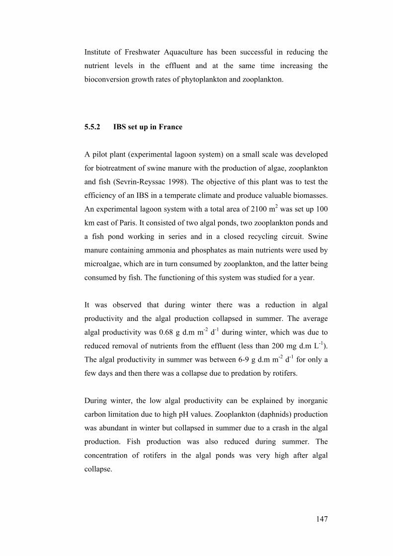
147

Institute of Freshwater Aquaculture has been successful in reducing the

nutrient levels in the effluent and at the same time increasing the

bioconversion growth rates of phytoplankton and zooplankton.

5.5.2 IBS set up in France

A pilot plant (experimental lagoon system) on a small scale was developed

for biotreatment of swine manure with the production of algae, zooplankton

and fish (Sevrin-Reyssac 1998). The objective of this plant was to test the

efficiency of an IBS in a temperate climate and produce valuable biomasses.

An experimental lagoon system with a total area of 2100 m2 was set up 100

km east of Paris. It consisted of two algal ponds, two zooplankton ponds and

a fish pond working in series and in a closed recycling circuit. Swine

manure containing ammonia and phosphates as main nutrients were used by

microalgae, which are in turn consumed by zooplankton, and the latter being

consumed by fish. The functioning of this system was studied for a year.

It was observed that during winter there was a reduction in algal

productivity and the algal production collapsed in summer. The average

algal productivity was 0.68 g d.m m-2 d-1 during winter, which was due to

reduced removal of nutrients from the effluent (less than 200 mg d.m L-1).

The algal productivity in summer was between 6-9 g d.m m-2 d-1 for only a

few days and then there was a collapse due to predation by rotifers.

During winter, the low algal productivity can be explained by inorganic

carbon limitation due to high pH values. Zooplankton (daphnids) production

was abundant in winter but collapsed in summer due to a crash in the algal

production. Fish production was also reduced during summer. The

concentration of rotifers in the algal ponds was very high after algal

collapse.

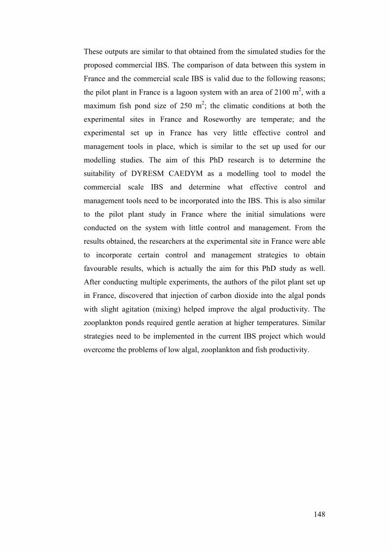
148

These outputs are similar to that obtained from the simulated studies for the

proposed commercial IBS. The comparison of data between this system in

France and the commercial scale IBS is valid due to the following reasons;

the pilot plant in France is a lagoon system with an area of 2100 m2, with a

maximum fish pond size of 250 m2; the climatic conditions at both the

experimental sites in France and Roseworthy are temperate; and the

experimental set up in France has very little effective control and

management tools in place, which is similar to the set up used for our

modelling studies. The aim of this PhD research is to determine the

suitability of DYRESM CAEDYM as a modelling tool to model the

commercial scale IBS and determine what effective control and

management tools need to be incorporated into the IBS. This is also similar

to the pilot plant study in France where the initial simulations were

conducted on the system with little control and management. From the

results obtained, the researchers at the experimental site in France were able

to incorporate certain control and management strategies to obtain

favourable results, which is actually the aim for this PhD study as well.

After conducting multiple experiments, the authors of the pilot plant set up

in France, discovered that injection of carbon dioxide into the algal ponds

with slight agitation (mixing) helped improve the algal productivity. The

zooplankton ponds required gentle aeration at higher temperatures. Similar

strategies need to be implemented in the current IBS project which would

overcome the problems of low algal, zooplankton and fish productivity.

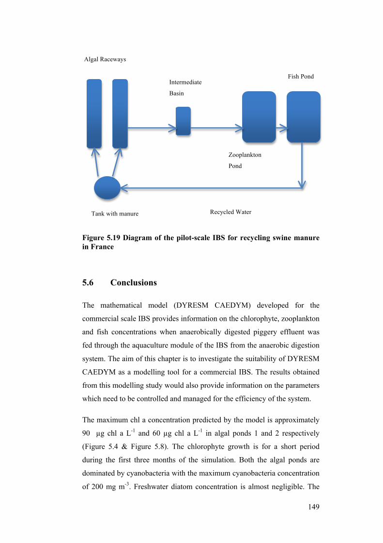
149

Figure 5.19 Diagram of the pilot-scale IBS for recycling swine manure in France

5.6 Conclusions

The mathematical model (DYRESM CAEDYM) developed for the

commercial scale IBS provides information on the chlorophyte, zooplankton

and fish concentrations when anaerobically digested piggery effluent was

fed through the aquaculture module of the IBS from the anaerobic digestion

system. The aim of this chapter is to investigate the suitability of DYRESM

CAEDYM as a modelling tool for a commercial IBS. The results obtained

from this modelling study would also provide information on the parameters

which need to be controlled and managed for the efficiency of the system.

The maximum chl a concentration predicted by the model is approximately

90 µg chl a L-1 and 60 µg chl a L-1 in algal ponds 1 and 2 respectively

(Figure 5.4 & Figure 5.8). The chlorophyte growth is for a short period

during the first three months of the simulation. Both the algal ponds are

dominated by cyanobacteria with the maximum cyanobacteria concentration

of 200 mg m-3. Freshwater diatom concentration is almost negligible. The

Algal Raceways

Fish Pond

Zooplankton

Pond

Tank with manure Recycled Water

Intermediate

Basin

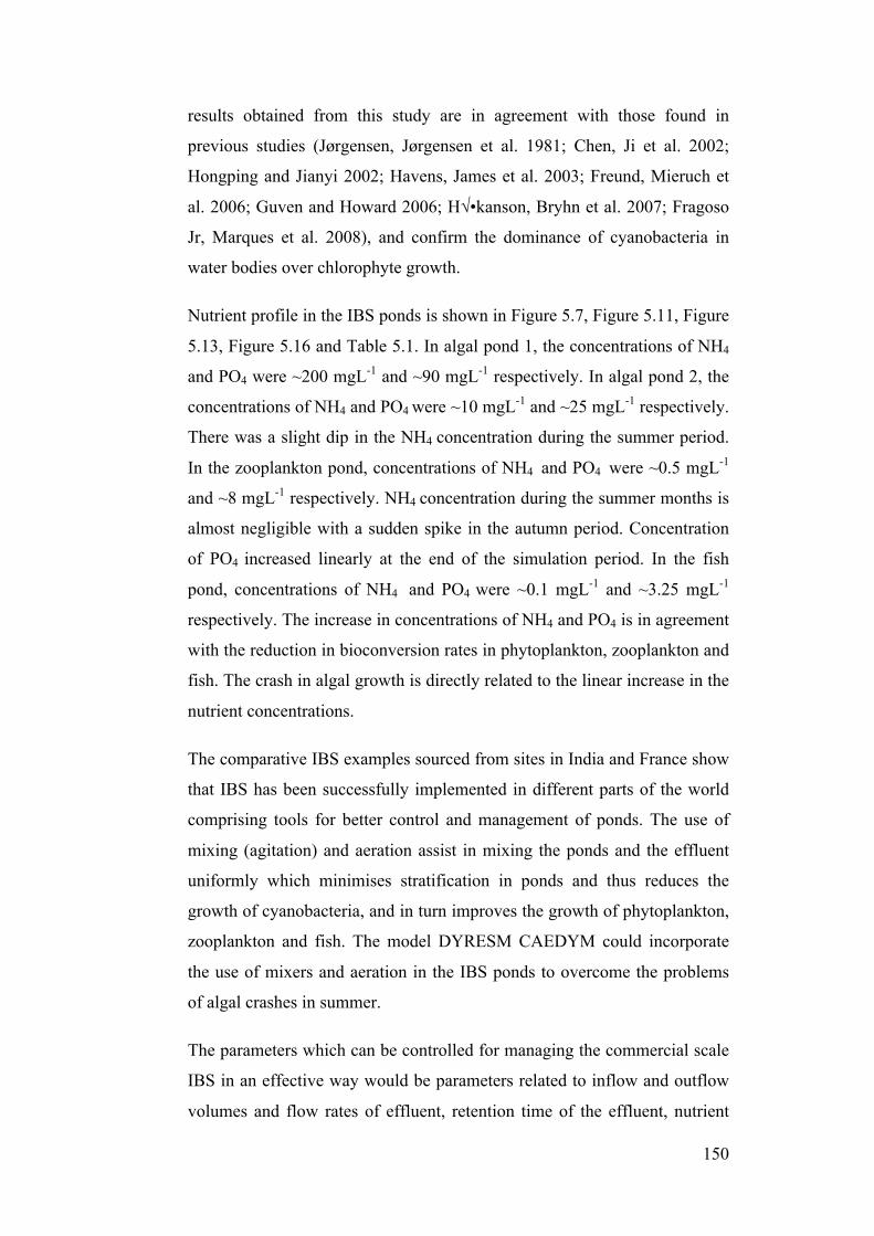
150

results obtained from this study are in agreement with those found in

previous studies (Jørgensen, Jørgensen et al. 1981; Chen, Ji et al. 2002;

Hongping and Jianyi 2002; Havens, James et al. 2003; Freund, Mieruch et

al. 2006; Guven and Howard 2006; H√•kanson, Bryhn et al. 2007; Fragoso

Jr, Marques et al. 2008), and confirm the dominance of cyanobacteria in

water bodies over chlorophyte growth.

Nutrient profile in the IBS ponds is shown in Figure 5.7, Figure 5.11, Figure

5.13, Figure 5.16 and Table 5.1. In algal pond 1, the concentrations of NH4

and PO4 were ~200 mgL-1 and ~90 mgL-1 respectively. In algal pond 2, the

concentrations of NH4 and PO4 were ~10 mgL-1 and ~25 mgL-1 respectively.

There was a slight dip in the NH4 concentration during the summer period.

In the zooplankton pond, concentrations of NH4 and PO4 were ~0.5 mgL-1

and ~8 mgL-1 respectively. NH4 concentration during the summer months is

almost negligible with a sudden spike in the autumn period. Concentration

of PO4 increased linearly at the end of the simulation period. In the fish

pond, concentrations of NH4 and PO4 were ~0.1 mgL-1 and ~3.25 mgL-1

respectively. The increase in concentrations of NH4 and PO4 is in agreement

with the reduction in bioconversion rates in phytoplankton, zooplankton and

fish. The crash in algal growth is directly related to the linear increase in the

nutrient concentrations.

The comparative IBS examples sourced from sites in India and France show

that IBS has been successfully implemented in different parts of the world

comprising tools for better control and management of ponds. The use of

mixing (agitation) and aeration assist in mixing the ponds and the effluent

uniformly which minimises stratification in ponds and thus reduces the

growth of cyanobacteria, and in turn improves the growth of phytoplankton,

zooplankton and fish. The model DYRESM CAEDYM could incorporate

the use of mixers and aeration in the IBS ponds to overcome the problems

of algal crashes in summer.




151





better module design.

The outputs from the modelling studies presented above were studied in a

sensitivity analysis presented in Chapter 6 in order to identify those critical

parameters which cause a significant change in the phytoplankton output

when subject to a variation. An auto calibration program is developed in

Chapter 7 which will be used to validate the model with real time data by

adjusting the parameters identified in the sensitivity analysis in Chapter 6.

152

6 Sensitivity Analysis

6.1 Introduction

A sensitivity analysis is used to determine how “sensitive” a model is to

changes in values of the parameters of the model and to changes in the

structure of the model. Parameter sensitivity is usually performed as a series

of tests in which the modeller sets different parameter values to see how a

change in the parameter causes a change in the dynamic behaviour of the

output. By showing how the model behaviour responds to changes in

parameter values, sensitivity analysis is a useful tool in model building as

well as in model evaluation, since it helps the modeller to understand the

dynamics of a system. Experimenting with a wide range of values can offer

insight into the behaviour of a system in any situation. Discovering that the

system behaviour greatly changes for a change in a parameter value can

identify a leverage point in the model- i.e. a parameter whose specific value

can significantly influence the behaviour mode of the system.

A sensitivity analysis also helps to build confidence in the model by

studying the uncertainties that are often associated with parameters in

models. Many parameters in system dynamics models represent quantities

that are very difficult, or even impossible to measure to a great deal of

accuracy in the real world. Also, some parameter values change in the real

world. Therefore, when building a system dynamics model, the modeller is

usually at least somewhat uncertain about the parameter values he chooses

and must use estimates. Sensitivity analysis allows determination of what

level of accuracy is necessary for a parameter to make the model

sufficiently useful and valid. If the tests reveal that the model is insensitive,

then it may be possible to use an estimate rather than a value with greater

precision. A sensitivity analysis can also indicate which parameter values

are reasonable to use in the model. If the model behaves as expected from

real world observations, it gives some indication that the parameter values

reflect, at least in part, the “real world.”

153

In Chapter 5 the suitability of DYRESM CAEDYM as a mathematical

model for the proposed commercial IBS was tested but the model could not

be validated with real time data because the IBS was not built at the time

this research was conducted. The purpose of developing the model was to

provide a quantitative description of the interactions that occur between

physical and ecological processes. DYRESM CAEDYM is a complex

model which has numerous interactive variables. The hydrodynamic

component DYRESM doesn’t require any site specific validation data,

however the ecological component CAEDYM requires calibration with field

data from the system which is being modelled. To minimise effort, it is

important to determine those parameters which the model result is most

sensitive to, then the calibration process should be directed towards these

parameters. Sensitivity studies form the basis for calibrating the parameters

for model validation. As the number of parameters which need to be

calibrated is large, a rigorous calibration method involving manual input of

parameters is not desired as this is time consuming. An automatic iterative

calibration program has been developed in Chapter 7 which automatically

validates the model with field data by adjusting the identified critical

parameters. A sensitivity analysis is conducted in this chapter to show how

sensitive the model outputs are to the selected parameters, which will assist

both the calibration discussed in Chapter 7 and the design and operation of

the aquaculture system.

154

6.2 Methods

Multiple studies have been conducted in the past regarding sensitivity

analysis for water quality models (Jørgensen, Jørgensen et al. 1981;

Jørgensen, Kamp-Nielsen et al. 1986), including DYRESM CAEDYM

(Schladow and Hamilton 1997). The assigned parameter range selected for

this sensitivity analysis study were obtained from Schladow and Hamilton

(1997) (Schladow and Hamilton 1997). The assigned values for the

parameters are the same values used in developing the model for the

proposed commercial IBS discussed in Chapter 5. These parameters were

also selected for the Auto Calibration routine to be discussed in Chapter 7.

Sensitivity analysis was conducted on the algal component of the IBS. The

sensitivity of model results to changed values of the parameters was

quantified with reference to chlorophyll a (Chl-a) growth. Chl-a growth was

considered to be one of the most important outputs for this research as it is

well correlated with biomass production in the proposed large scale IBS.

For the sensitivity analysis, the model was run with each of the parameters

in Table 6.2 using the assigned value, the minimum (-10% of assigned

value) and the maximum (+10% of the assigned value) while the other

parameters were kept fixed at the assigned value. The model was run for a

period of 365 days, starting from 1st June 2006 to 31st May 2007.

The working formulae for the values chosen are shown below.

Minimum Value = Assigned Value – (10% of Assigned Value) Eq. 6.1

Maximum Value = Assigned Value + (10% of Assigned Value) Eq. 6.2

% Range = 100 – [(Minimum Value/Maximum Value)*100] Eq. 6.3

The assigned values were selected from Schladow and Hamilton (1997).

The minimum and maximum values were computed as 10% of the assigned

values to show a distribution range of these parameters and their effects on

the chl-a output.

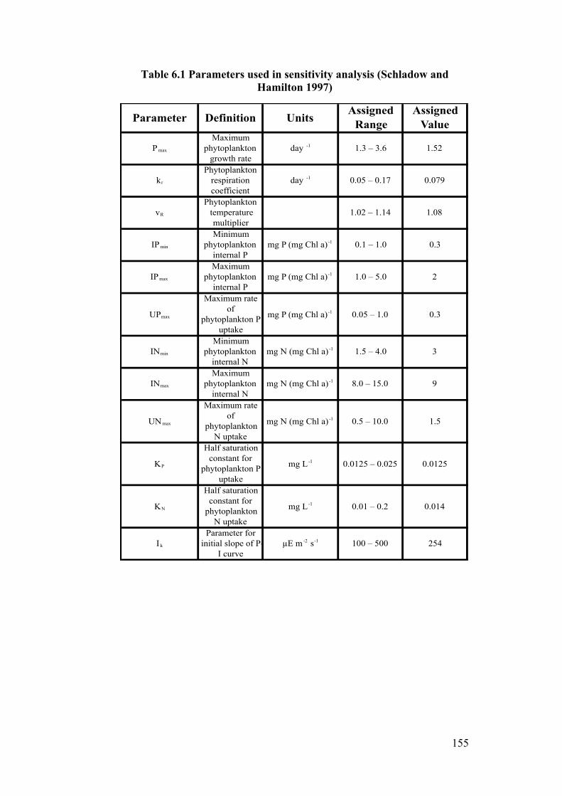
155

Table 6.1 Parameters used in sensitivity analysis (Schladow and Hamilton 1997)

Parameter Definition UnitsAssigned

RangeAssigned

Value

P max

Maximum phytoplankton

growth rateday -1 1.3 – 3.6 1.52

kr

Phytoplankton respiration coefficient

day -1 0.05 – 0.17 0.079

vR

Phytoplankton temperature multiplier

1.02 – 1.14 1.08

IPmin

Minimum phytoplankton

internal Pmg P (mg Chl a)-1 0.1 – 1.0 0.3

IPmax


internal Pmg P (mg Chl a)-1 1.0 – 5.0 2

UPmax

Maximum rate of

phytoplankton P uptake

mg P (mg Chl a)-1 0.05 – 1.0 0.3

INmin

Minimum phytoplankton

internal Nmg N (mg Chl a)-1 1.5 – 4.0 3

INmax


internal Nmg N (mg Chl a)-1 8.0 – 15.0 9

UNmax

Maximum rate of

phytoplankton N uptake

mg N (mg Chl a)-1 0.5 – 10.0 1.5

KP

Half saturation constant for

phytoplankton P uptake

mg L-1 0.0125 – 0.025 0.0125

KN

Half saturation constant for

phytoplankton N uptake

mg L-1 0.01 – 0.2 0.014

Ik

Parameter for initial slope of P-

I curveµE m-2 s-1 100 – 500 254

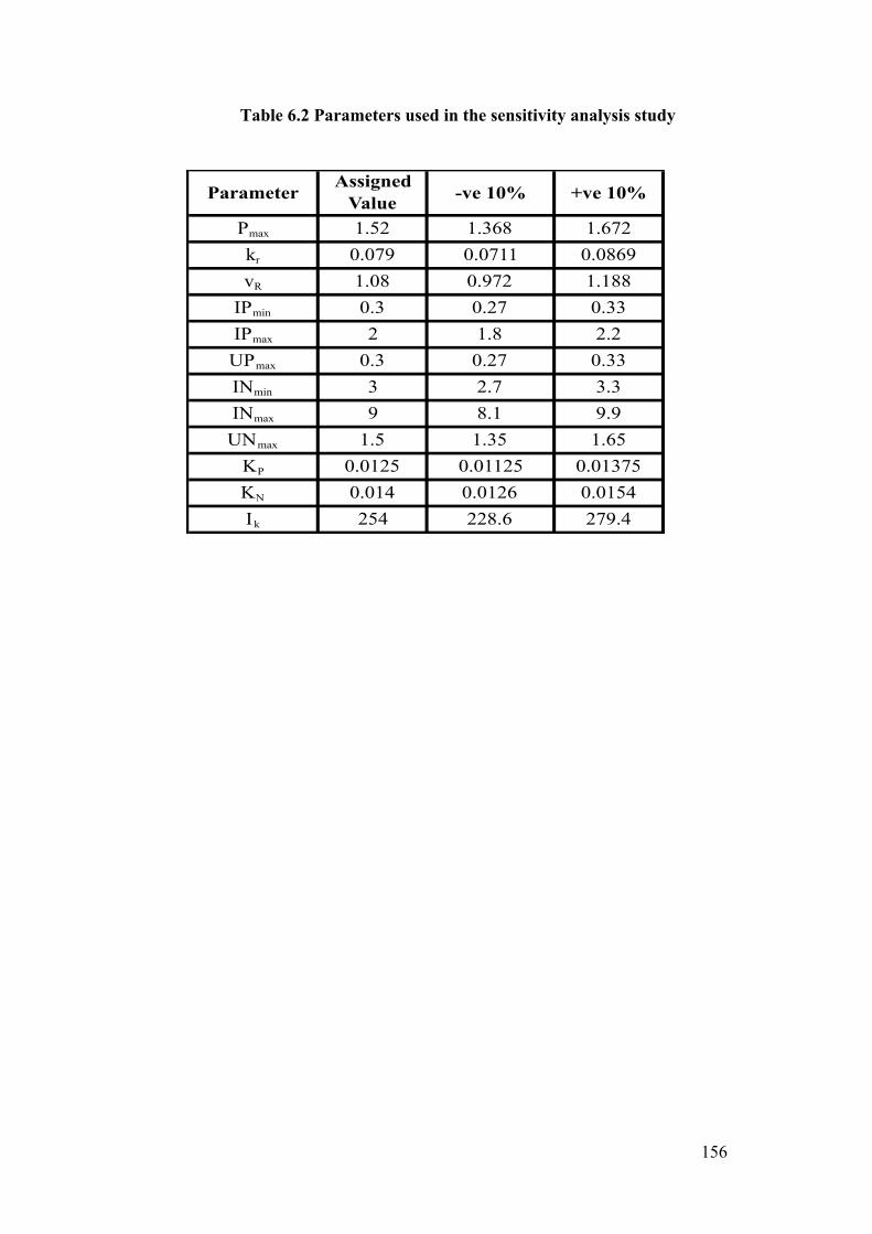
156

Table 6.2 Parameters used in the sensitivity analysis study

ParameterAssigned

Value -ve 10% +ve 10%

Pmax 1.52 1.368 1.672kr 0.079 0.0711 0.0869vR 1.08 0.972 1.188IPmin 0.3 0.27 0.33IPmax 2 1.8 2.2UPmax 0.3 0.27 0.33INmin 3 2.7 3.3INmax 9 8.1 9.9UNmax 1.5 1.35 1.65KP 0.0125 0.01125 0.01375KN 0.014 0.0126 0.0154Ik 254 228.6 279.4

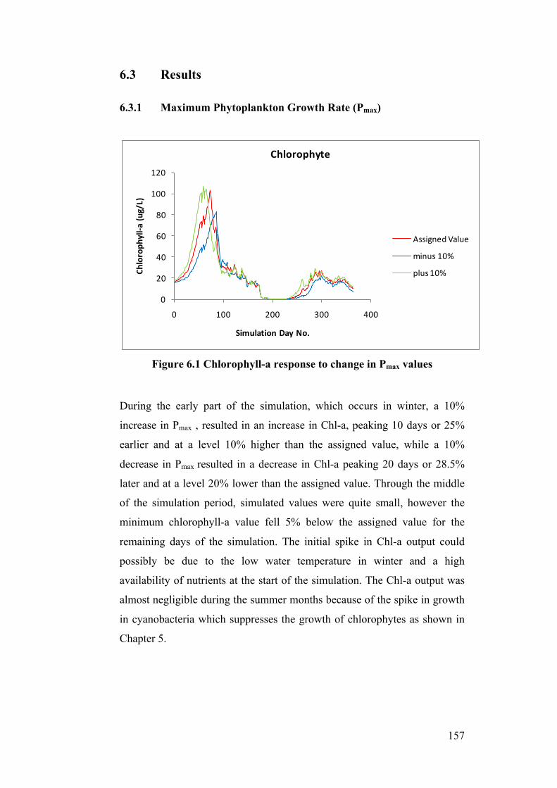
157

6.3 Results

6.3.1 Maximum Phytoplankton Growth Rate (Pmax)

Figure 6.1 Chlorophyll-a response to change in Pmax values

During the early part of the simulation, which occurs in winter, a 10%

increase in Pmax , resulted in an increase in Chl-a, peaking 10 days or 25%

earlier and at a level 10% higher than the assigned value, while a 10%

decrease in Pmax resulted in a decrease in Chl-a peaking 20 days or 28.5%

later and at a level 20% lower than the assigned value. Through the middle

of the simulation period, simulated values were quite small, however the

minimum chlorophyll-a value fell 5% below the assigned value for the

remaining days of the simulation. The initial spike in Chl-a output could

possibly be due to the low water temperature in winter and a high

availability of nutrients at the start of the simulation. The Chl-a output was

almost negligible during the summer months because of the spike in growth

in cyanobacteria which suppresses the growth of chlorophytes as shown in

Chapter 5.

0

20

40

60

80

100

120

0 100 200 300 400

Chloroph

yll-‐a (u

g/L)

Simulation Day No.

Chlorophyte

Assigned Value

minus 10%

plus 10%

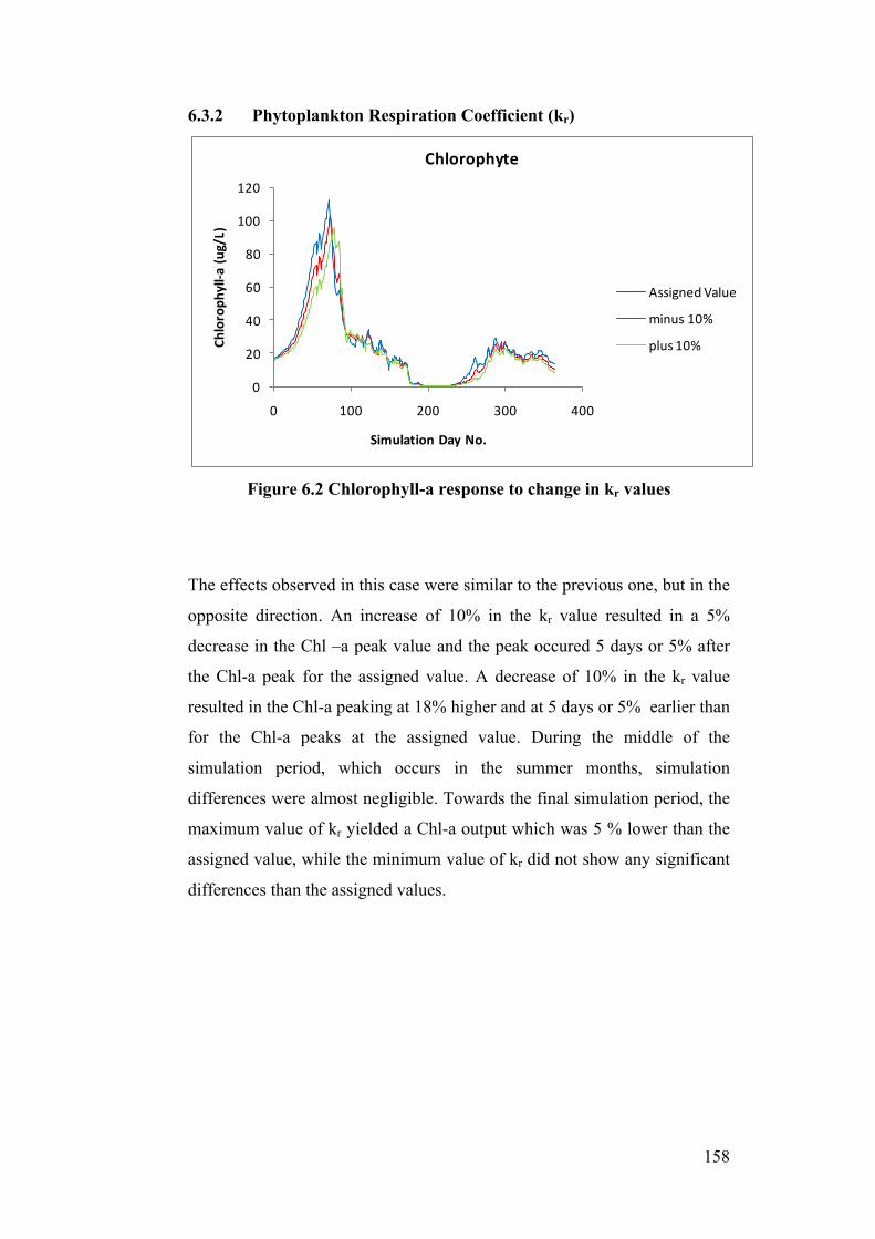
158

6.3.2 Phytoplankton Respiration Coefficient (kr)

Figure 6.2 Chlorophyll-a response to change in kr values

The effects observed in this case were similar to the previous one, but in the

opposite direction. An increase of 10% in the kr value resulted in a 5%

decrease in the Chl –a peak value and the peak occured 5 days or 5% after

the Chl-a peak for the assigned value. A decrease of 10% in the kr value

resulted in the Chl-a peaking at 18% higher and at 5 days or 5% earlier than

for the Chl-a peaks at the assigned value. During the middle of the

simulation period, which occurs in the summer months, simulation

differences were almost negligible. Towards the final simulation period, the

maximum value of kr yielded a Chl-a output which was 5 % lower than the

assigned value, while the minimum value of kr did not show any significant

differences than the assigned values.

0

20

40

60

80

100

120

0 100 200 300 400

Chloroph

yll-‐a (u

g/L)

Simulation Day No.

Chlorophyte

Assigned Value

minus 10%

plus 10%

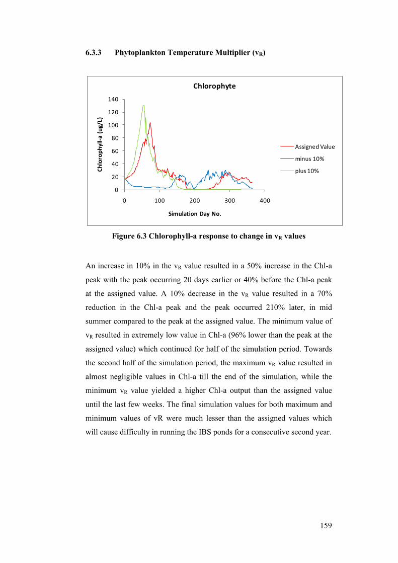
159

6.3.3 Phytoplankton Temperature Multiplier (vR)

Figure 6.3 Chlorophyll-a response to change in vR values

An increase in 10% in the vR value resulted in a 50% increase in the Chl-a

peak with the peak occurring 20 days earlier or 40% before the Chl-a peak

at the assigned value. A 10% decrease in the vR value resulted in a 70%

reduction in the Chl-a peak and the peak occurred 210% later, in mid

summer compared to the peak at the assigned value. The minimum value of

vR resulted in extremely low value in Chl-a (96% lower than the peak at the

assigned value) which continued for half of the simulation period. Towards

the second half of the simulation period, the maximum vR value resulted in

almost negligible values in Chl-a till the end of the simulation, while the

minimum vR value yielded a higher Chl-a output than the assigned value

until the last few weeks. The final simulation values for both maximum and

minimum values of vR were much lesser than the assigned values which

will cause difficulty in running the IBS ponds for a consecutive second year.

0

20

40

60

80

100

120

140

0 100 200 300 400

Chloroph

yll-‐a (u

g/L)

Simulation Day No.

Chlorophyte

Assigned Value

minus 10%

plus 10%

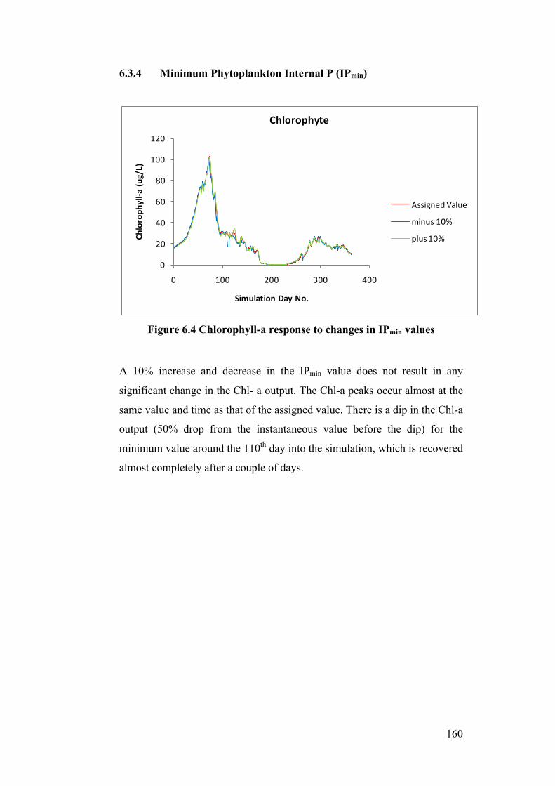
160

6.3.4 Minimum Phytoplankton Internal P (IPmin)

Figure 6.4 Chlorophyll-a response to changes in IPmin values

A 10% increase and decrease in the IPmin value does not result in any

significant change in the Chl- a output. The Chl-a peaks occur almost at the

same value and time as that of the assigned value. There is a dip in the Chl-a

output (50% drop from the instantaneous value before the dip) for the

minimum value around the 110th day into the simulation, which is recovered

almost completely after a couple of days.

0

20

40

60

80

100

120

0 100 200 300 400

Chloroph

yll-‐a (u

g/L)

Simulation Day No.

Chlorophyte

Assigned Value

minus 10%

plus 10%

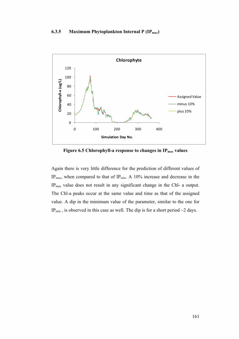
161

6.3.5 Maximum Phytoplankton Internal P (IPmax)

Figure 6.5 Chlorophyll-a response to changes in IPmax values

Again there is very little difference for the prediction of different values of

IPmax, when compared to that of IPmin. A 10% increase and decrease in the

IPmax value does not result in any significant change in the Chl- a output.

The Chl-a peaks occur at the same value and time as that of the assigned

value. A dip in the minimum value of the parameter, similar to the one for

IPmin , is observed in this case as well. The dip is for a short period ~2 days.

0

20

40

60

80

100

120

0 100 200 300 400

Chloroph

yll-‐a (u

g/L)

Simulation Day No.

Chlorophyte

Assigned Value

minus 10%

plus 10%

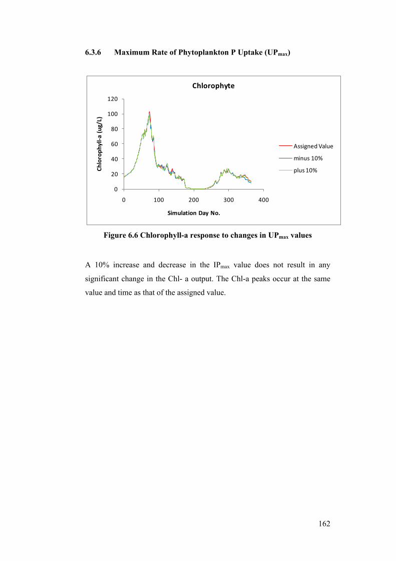
162

6.3.6 Maximum Rate of Phytoplankton P Uptake (UPmax)

Figure 6.6 Chlorophyll-a response to changes in UPmax values

A 10% increase and decrease in the IPmax value does not result in any

significant change in the Chl- a output. The Chl-a peaks occur at the same

value and time as that of the assigned value.

0

20

40

60

80

100

120

0 100 200 300 400

Chloroph

yll-‐a (u

g/L)

Simulation Day No.

Chlorophyte

Assigned Value

minus 10%

plus 10%

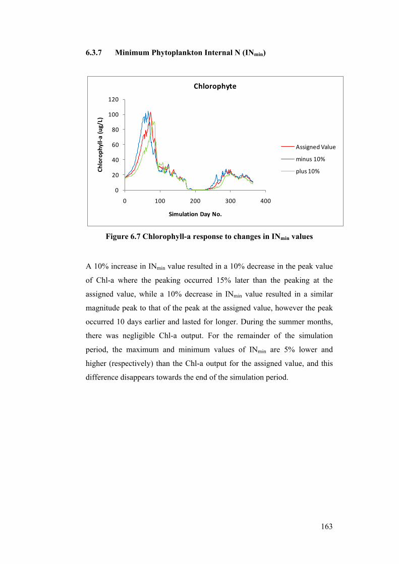
163

6.3.7 Minimum Phytoplankton Internal N (INmin)

Figure 6.7 Chlorophyll-a response to changes in INmin values

A 10% increase in INmin value resulted in a 10% decrease in the peak value

of Chl-a where the peaking occurred 15% later than the peaking at the

assigned value, while a 10% decrease in INmin value resulted in a similar

magnitude peak to that of the peak at the assigned value, however the peak

occurred 10 days earlier and lasted for longer. During the summer months,

there was negligible Chl-a output. For the remainder of the simulation

period, the maximum and minimum values of INmin are 5% lower and

higher (respectively) than the Chl-a output for the assigned value, and this

difference disappears towards the end of the simulation period.

0

20

40

60

80

100

120

0 100 200 300 400

Chloroph

yll-‐a (u

g/L)

Simulation Day No.

Chlorophyte

Assigned Value

minus 10%

plus 10%

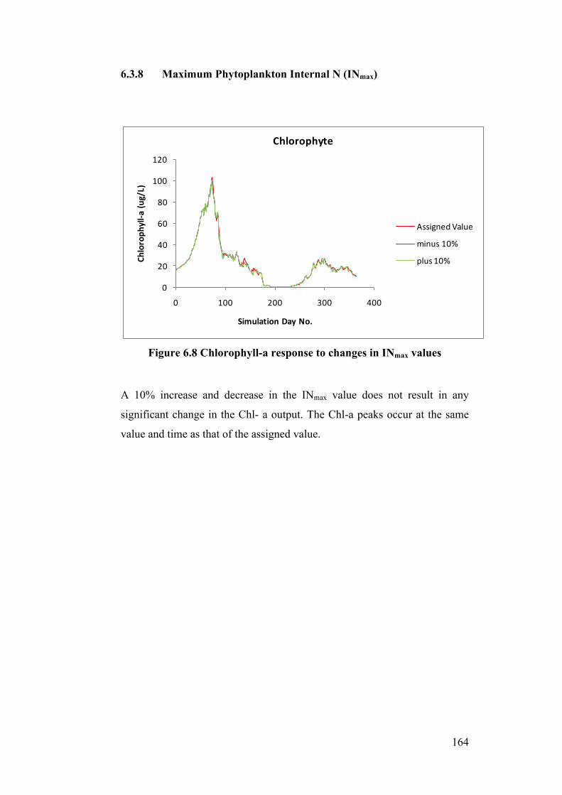
164

6.3.8 Maximum Phytoplankton Internal N (INmax)

Figure 6.8 Chlorophyll-a response to changes in INmax values

A 10% increase and decrease in the INmax value does not result in any


value and time as that of the assigned value.

0

20

40

60

80

100

120

0 100 200 300 400

Chloroph

yll-‐a (u

g/L)

Simulation Day No.

Chlorophyte

Assigned Value

minus 10%

plus 10%

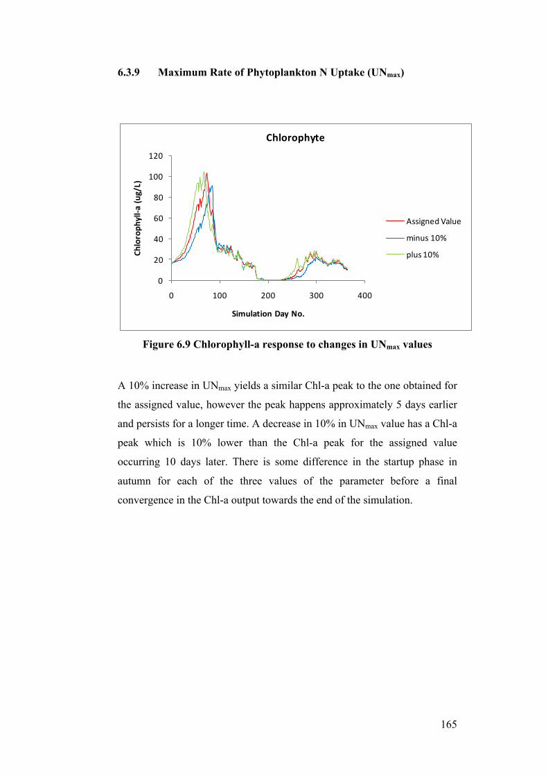
165

6.3.9 Maximum Rate of Phytoplankton N Uptake (UNmax)

Figure 6.9 Chlorophyll-a response to changes in UNmax values

A 10% increase in UNmax yields a similar Chl-a peak to the one obtained for

the assigned value, however the peak happens approximately 5 days earlier

and persists for a longer time. A decrease in 10% in UNmax value has a Chl-a

peak which is 10% lower than the Chl-a peak for the assigned value

occurring 10 days later. There is some difference in the startup phase in

autumn for each of the three values of the parameter before a final

convergence in the Chl-a output towards the end of the simulation.

0

20

40

60

80

100

120

0 100 200 300 400

Chloroph

yll-‐a (u

g/L)

Simulation Day No.

Chlorophyte

Assigned Value

minus 10%

plus 10%

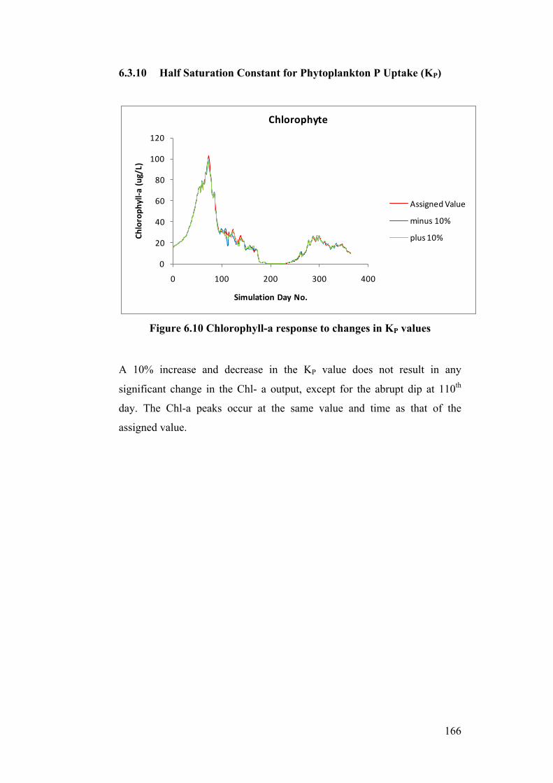
166

6.3.10 Half Saturation Constant for Phytoplankton P Uptake (KP)

Figure 6.10 Chlorophyll-a response to changes in KP values

A 10% increase and decrease in the KP value does not result in any

significant change in the Chl- a output, except for the abrupt dip at 110th

day. The Chl-a peaks occur at the same value and time as that of the

assigned value.

0

20

40

60

80

100

120

0 100 200 300 400

Chloroph

yll-‐a (u

g/L)

Simulation Day No.

Chlorophyte

Assigned Value

minus 10%

plus 10%

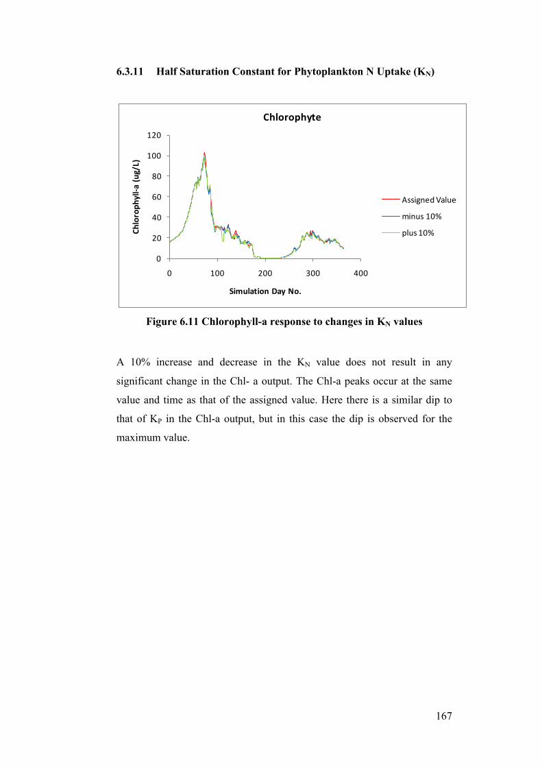
167

6.3.11 Half Saturation Constant for Phytoplankton N Uptake (KN)

Figure 6.11 Chlorophyll-a response to changes in KN values

A 10% increase and decrease in the KN value does not result in any


value and time as that of the assigned value. Here there is a similar dip to

that of KP in the Chl-a output, but in this case the dip is observed for the

maximum value.

0

20

40

60

80

100

120

0 100 200 300 400

Chloroph

yll-‐a (u

g/L)

Simulation Day No.

Chlorophyte

Assigned Value

minus 10%

plus 10%

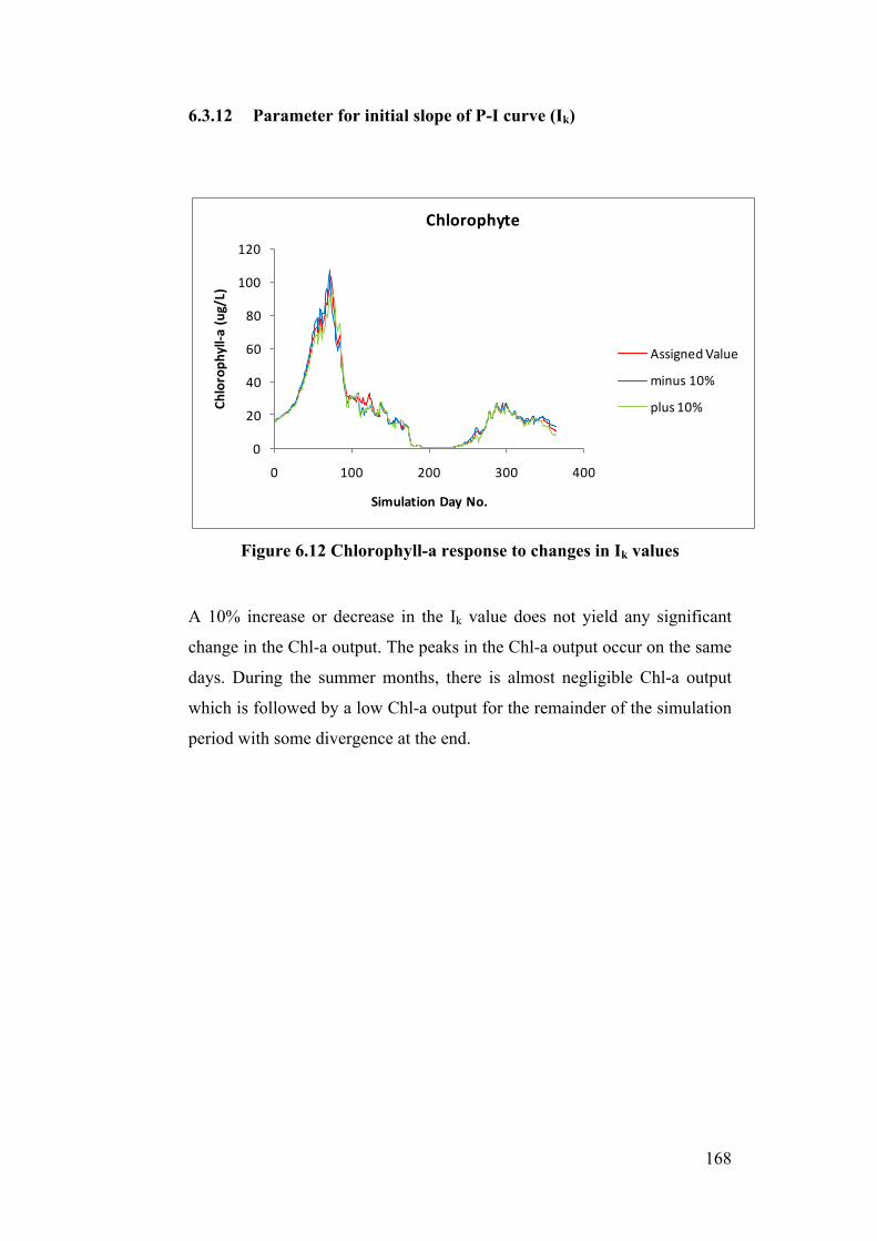
168

6.3.12 Parameter for initial slope of P-I curve (Ik)

Figure 6.12 Chlorophyll-a response to changes in Ik values

A 10% increase or decrease in the Ik value does not yield any significant

change in the Chl-a output. The peaks in the Chl-a output occur on the same

days. During the summer months, there is almost negligible Chl-a output

which is followed by a low Chl-a output for the remainder of the simulation

period with some divergence at the end.

0

20

40

60

80

100

120

0 100 200 300 400

Chloroph

yll-‐a (u

g/L)

Simulation Day No.

Chlorophyte

Assigned Value

minus 10%

plus 10%

169

6.4 Discussion

Sensitivity analysis is the study of how the variation (uncertainty) in the

output of a mathematical model can be qualitatively or quantitatively

measured, to different sources of variation in the input of the model. It is a

technique for systematically changing parameters in a model to determine

the effects of such changes. In more general terms uncertainty and

sensitivity analysis investigate the robustness of a study when the study

includes some form of mathematical modelling. Sensitivity analysis can be

useful to mathematical modellers for a range of purposes including:

• decision making or the development of recommendations for

decision makers (e.g. testing the robustness of a result);

• enhancing communication from modellers to decision makers (e.g.

by making recommendations more credible, understandable,

compelling or persuasive);

• increased understanding or quantification of the system (e.g.

understanding relationships between input and output variables); and

• model development (e.g. searching for errors in the model).

The outputs (Figure 6.1 to Figure 6.12) show that the model results for

chlorophyll-a are sensitive to a relatively small subset of parameters.

Parameters for which chlorophyll-a is highly sensitive are those that directly

alter growth rates i.e. maximum phytoplankton growth rate (Pmax),

phytoplankton respiration coefficient (kr) and phytoplankton temperature

multiplier (vR), or indirectly affect growth rates through their ability to

utilise nitrogen (INmin and UNmax). These results are in agreement with the

results presented in (Hamilton and Schladow 1997) where chl-a was highly

sensitive for maximum phytoplankton growth rate and phytoplankton

respiration rate. However in Hamilton and Schladow (Hamilton and

Schladow 1997) chl-a is sensitive to IPmin and UPmax i.e. parameters that

indirectly affect growth rates through their ability to utilise phosphorus as

opposed to INmin and UNmax in the IBS ponds. This could be due to the IBS

system being a nitrogen limited system.

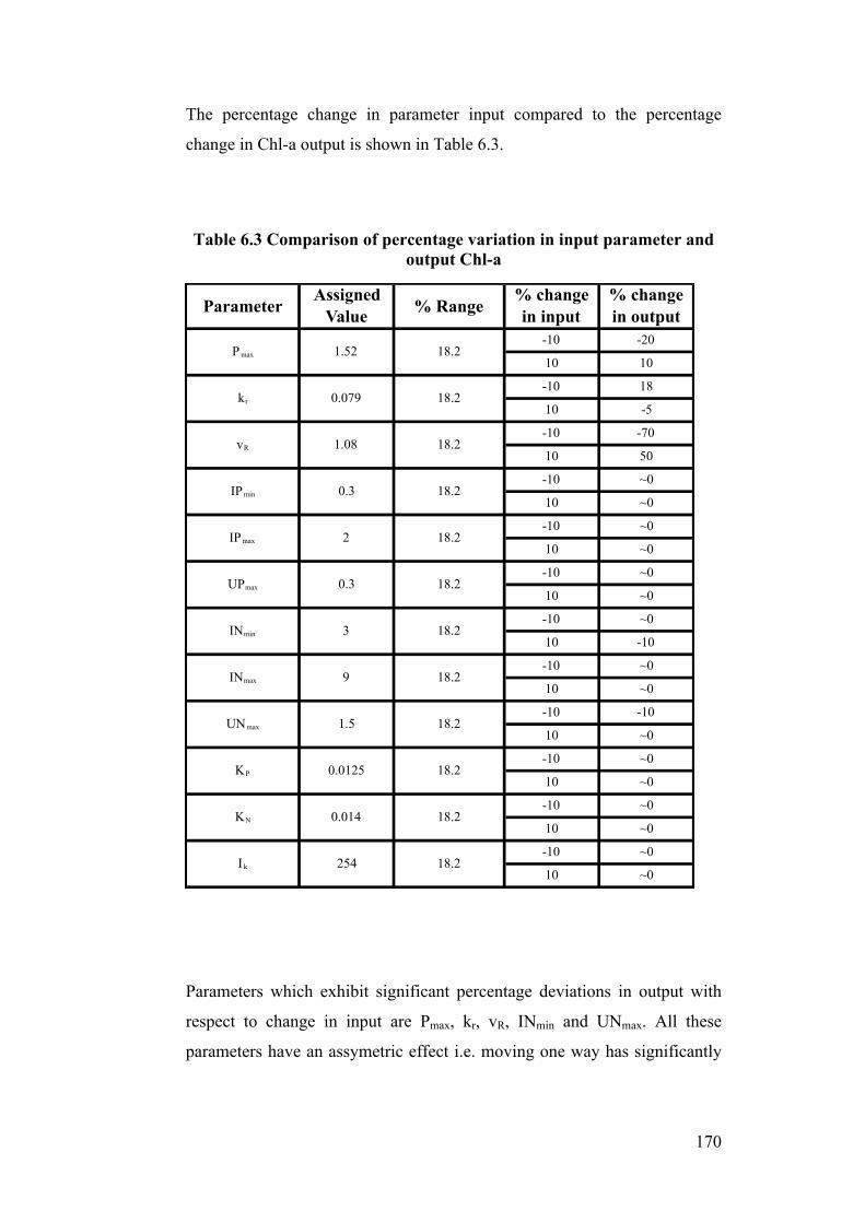
170

The percentage change in parameter input compared to the percentage

change in Chl-a output is shown in Table 6.3.

Table 6.3 Comparison of percentage variation in input parameter and output Chl-a

Parameters which exhibit significant percentage deviations in output with

respect to change in input are Pmax, kr, vR, INmin and UNmax. All these

parameters have an assymetric effect i.e. moving one way has significantly

ParameterAssigned

Value % Range% change in input

% change in output

-10 -20

10 10

-10 18

10 -5

-10 -70

10 50

-10 ~0

10 ~0

-10 ~0

10 ~0

-10 ~0

10 ~0

-10 ~0

10 -10

-10 ~0

10 ~0

-10 -10

10 ~0

-10 ~0

10 ~0

-10 ~0

10 ~0

-10 ~0

10 ~0Ik 254 18.2

KP 0.0125 18.2

KN 0.014 18.2

INmax 9 18.2

UNmax 1.5 18.2

UPmax 0.3 18.2

INmin 3 18.2

IPmin 0.3 18.2

IPmax 2 18.2

kr 0.079 18.2

vR 1.08 18.2

Pmax 1.52 18.2

171

less effect than moving the other way. This shows that there is an optimum

somewhere between the two points.

6.5 Conclusions and Further Work

This study provided an overview of a selected group of parameters which

are most sensitive to chlorophyll-a output. This technique can be applied to

the commercial IBS, when constructed, in future. The sensitivity of different

outputs can be tested against a combination of different parameters for the

IBS which can assist the modeller in deciding which parameters need to be

altered to expect a different output, and which parameters can be altered

without expecting any change in the output. This mechanism would provide

effective control and management of the IBS from a modeller’s perspective.

Further investigation needs to be done on the response of different outputs

e.g. cyanobacteria, freshwater diatoms, zooplankton, fish growth etc with

changes in the parameters selected for this study. This is useful in

identifying the parameters which are most sensitive to a particular output.

However when the number of parameters increases along with a variety of

outputs to be assessed, a manual method of altering parameter values to

observe the change in output is time consuming and more of a “trial and

error” approach. Also this sensitivity study relies on using the minimum,

maximum and mean values of the parameters selected without observing

any changes in the intermediate values, i.e. observing any changes in the

output during incremental changes to the selected parameter. This

incremental change is required when field data needs to be validated against

the simulated data. It is obvious that manually inputting the values with

incremental changes would be an extremely time consuming and frustrating

process. Therefore a need for development of an efficient automatic

calibration process is required, which has been developed in Chapter 7.

172

7 Automated Parameter Estimation and

Calibration

7.1 Introduction

Automatic calibration is a mathematical technique employed by scientists,

engineers and mathematical modellers to calibrate and validate a

mathematical model to obtain realistic data. The fundamental way is to alter

the variable parameters of a model and compare the outputs with the

obtained field (actual) data. The parameter value which gives the closest fit

(agreement) of the field data to the simulated data is chosen to represent that

value. In simple models, which require minimum number of parameters,

calibration and validation can be done manually as long as it doesn’t

consume much time. However in complex models, like DYRESM

CAEDYM, where a large number of parameters, either singularly or in

conjunction, have a profound effect on the outputs, manual calibration is

lengthy, tedious and an inefficient process. Often, this would lead to

erroneous and inconsistent results, which would misguide the modellers and

operational engineers. Therefore a method of automated calibration which

includes model validation and parameter estimation by using automated

computer programs is very useful in these circumstances. This provides the

advantage of running a more sophisticated process, reduces the chances of

errors and false estimations and is less tedious and taxing as opposed to the

conventional manual methods.

In Chapter 6 a sensitivity analysis study was conducted on selected

parameters for the proposed large scale IBS model. The sensitivity analysis

yielded valuable information about the response of chlorophyll-a output to

fixed positive and negative variations to those parameters. This paved a way

for calibrating the model with real time data. However there is a need for

effectively calibrating a model like DYRESM CAEDYM which has been

discussed in Section 6.5. This chapter introduces a method to calibrate the

proposed large scale IBS model using an automatic calibration program

173

which fits the simulated model output to the field data by varying the

parameters selected.

7.2 Methods

7.2.1 Incorporating Monte Carlo and GLUE calibration in

DYRESM CAEDYM

A calibration routine involving Bayesian Monte Carlo method and GLUE

was set up to enable automated parameter calibration in DYRESM

CAEDYM. Both the Bayesian Monte Carlo and GLUE method have been

discussed in Chapter 2. The GLUE procedure explicitly recognizes the

equivalence or near equivalence of different parameter sets or model

structures in the representation of hydrological responses (Beven and Binley

1992). The parameters selected for the calibration were

1) Maximum Potential Growth Rate of Phytoplankton (Pmax)

2) Parameter for initial slope of P_I curve (IK)

3) Half Saturation Constant for Nitrogen (KN)

4) Half Saturation Constant for Phosphorus (KP)

5) Internal Minimum Phosphorus (IPmin)

6) Internal Maximum Phosphorus (IPmax)

7) Maximum Rate of Phytoplankton Phosphorus Uptake (UPmax)

8) Internal Minimum Nitrogen (INmin)

9) Internal Maximum Nitrogen (INmax)

10) Maximum Rate of Phytoplankton Nitrogen Uptake (UNmax)

11) Respiration Rate (kr)

These parameters were determined using initial simulation studies to limit

the bounds of the parameter space to reduce over parameterization. Ranges

174

for the above parameters were obtained from literature (Hamilton and

Schladow 1997; Schladow and Hamilton 1997). Due to the unavailability of

real time field data, pseudo field data was generated with random values for

demonstration purpose for this calibration routine to function properly.

7.2.2 Analysis of the auto calibration program

The calibration program comprises of a main program which has several

subroutines embedded within it. These subroutines perform individual tasks

for the calibration routine to function properly. The sequence of the program

execution is explained below:

1. The program first aligns the numerical values in the water quality

parameters file to match that of an 80 character set. This is done so

that specific parameter values can be inserted at the appropriate

fields in the water quality parameters file, without causing the

DYRESM CAEDYM program to crash. It has been observed that

insertion of parameter values at different fields in the parameters file

causes the model to crash. Subroutine ReformatDYCD.f90 transfers

the parameters from “WQParameters.dat” file to “dycd.dat” file

according to the 80 character alignment. The new “dycd.dat” file is

used for running the model simulations. This alignment needs to be

done only once before the start of the initial simulations.

2. The main program Driver.f90 consists of three subroutines

• datamod.f90

• master_run.f90

• glue_sub.f90

The main program Driver.f90 is executed in the following sequence:

First the number of simulations to be conducted is entered. For

demonstration purposes the number of simulations is set at 1000. Large

number of simulations requires longer computing times. A randomised

value (within the estimated limits) is selected for each of the 11

parameters selected for calibration. These values are stored in the new

“dycd.dat” file which will be used for CAEDYM simulations. A nested

175

loop performs this function using the datamod.f90 and the num_ascii.f90

subroutines. This subroutine places the parameter at the exact position in

the “dycd.dat” file. It is extremely important to place these values at the

exact position else CAEDYM will crash during the simulations.

The next part of the code is the subroutine master_run.f90. This

subroutine calls for the program DYRESM CAEDYM to run.

The final part of the code is the GLUE (Monte Carlo) calibration,

executed by the glue_sub subroutine. Once DYRESM CAEDYM

simulations are completed, GLUE calibration is executed. Chlorophyte

and cyanobacteria concentration outputs are chosen for demonstration

purposes. CAEDYM stores the simulated chlorophyte and cyanobacteria

data in “CHLOR.ITS” and “CYANO.ITS” files as Integrated Time

Series (ITS) files. A pseudo field data is randomly created for

demonstration of the program. Both the pseudo field and the simulated

data files are opened and GLUE calibration is performed where the

Nash-Sutcliffe coefficient (NS) is calculated. The numerical values of

the parameter along with the NS value for that particular parameter

combination is written to a text file for later comparison.

The above sequence is repeated for the total number of simulations (i.e.

1000 in this case). For each simulation, the NS values are recorded with

the parameter value combination. At the end of the simulation period,

the parameter combination which gives the NS value closest to 1.0 will

give the best fit with the field data. A flowchart describing the above

sequence is shown in Figure 7.1.

The program code written in FORTRAN 90 is shown in Appendix E. A

GLUE calibration output of 10 simulations is shown in Appendix F.

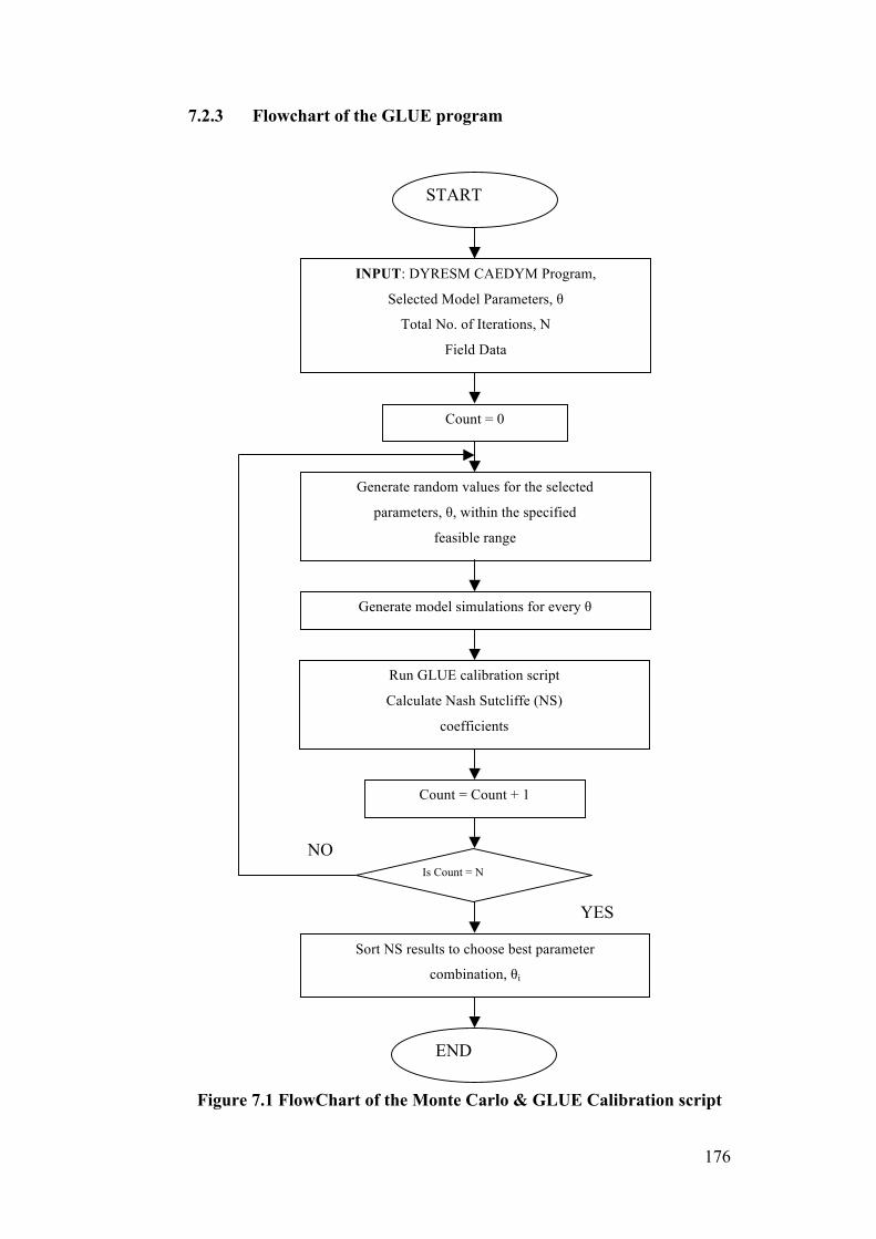
176

7.2.3 Flowchart of the GLUE program

Figure 7.1 FlowChart of the Monte Carlo & GLUE Calibration script

NO

YES

Is Count = N

Sort NS results to choose best parameter

combination, θi

END

Generate model simulations for every θ

Run GLUE calibration script

Calculate Nash Sutcliffe (NS)

coefficients

Count = Count + 1

Generate random values for the selected

parameters, θ, within the specified

feasible range

Count = 0

START

INPUT: DYRESM CAEDYM Program,

Selected Model Parameters, θ

Total No. of Iterations, N

Field Data

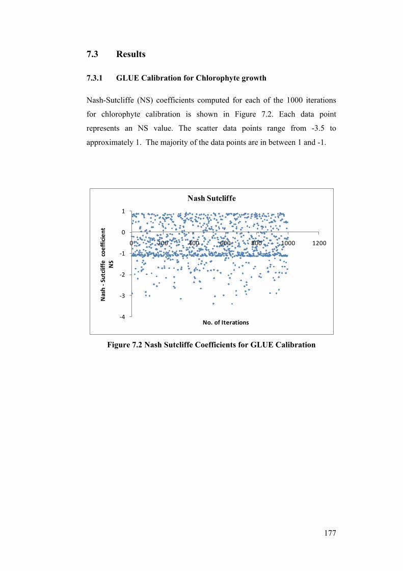
177

7.3 Results

7.3.1 GLUE Calibration for Chlorophyte growth

Nash-Sutcliffe (NS) coefficients computed for each of the 1000 iterations

for chlorophyte calibration is shown in Figure 7.2. Each data point

represents an NS value. The scatter data points range from -3.5 to

approximately 1. The majority of the data points are in between 1 and -1.

Figure 7.2 Nash Sutcliffe Coefficients for GLUE Calibration

-‐4

-‐3

-‐2

-‐1

0

1

0 200 400 600 800 1000 1200

Nash -‐Sutcliffe

coe

fficie

ntNS

No. of Iterations

Nash Sutcliffe

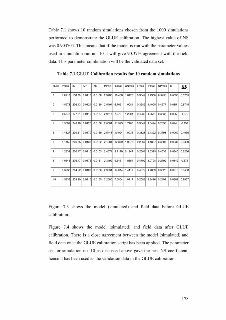
178

Table 7.1 shows 10 random simulations chosen from the 1000 simulations

performed to demonstrate the GLUE calibration. The highest value of NS

was 0.903704. This means that if the model is run with the parameter values

used in simulation run no. 10 it will give 90.37% agreement with the field

data. This parameter combination will be the validated data set.

Table 7.1 GLUE Calibration results for 10 random simulations

Figure 7.3 shows the model (simulated) and field data before GLUE

calibration.

Figure 7.4 shows the model (simulated) and field data after GLUE

calibration. There is a close agreement between the model (simulated) and

field data once the GLUE calibration script has been applied. The parameter

set for simulation no. 10 as discussed above gave the best NS coefficient,

hence it has been used as the validation data in the GLUE calibration.

Runs Pmax IK KP KN INmin INmax UNmax IPmin IPmax UPmax kr NS

1 1.6916 168.76 0.0115 0.0108 2.9488 10.406 1.0426 0.3649 2.7350 0.3453 0.0893 0.5255

2 1.5978 206.13 0.0124 0.0130 2.5194 6.702 1.0081 0.3282 1.1005 0.4977 0.085 0.8715

3 0.5846 177.91 0.0110 0.0157 2.9517 7.270 1.2204 0.4289 1.2571 0.3336 0.095 - 1.079

4 1.3099 248.48 0.0120 0.0136 2.0501 11.923 1.7405 0.3344 1.8494 0.2858 0.094 - 0.157

5 1.4327 209.31 0.0179 0.0169 2.5443 10.924 1.0936 0.3828 2.4322 0.3798 0.0969 0.4035

6 1.1459 200.65 0.0136 0.0102 2.1284 12.879 1.9878 0.2067 1.4837 0.3807 0.0937 0.0389

7 1.2831 206.47 0.0110 0.0153 2.4674 9.7179 0.1247 0.2601 1.5325 0.4538 0.0845 0.8236

8 1.0641 276.47 0.0176 0.0161 2.3192 9.346 1.0351 0.4792 1.0798 0.2792 0.0842 - 0.376

9 1.3235 294.22 0.0108 0.0156 2.9931 14.014 1.4117 0.4079 1.7869 0.3526 0.0913 0.6438

10 1.5238 239.20 0.0110 0.0155 2.2686 7.6804 1.0117 0.2583 2.8496 0.2192 0.0881 0.9037

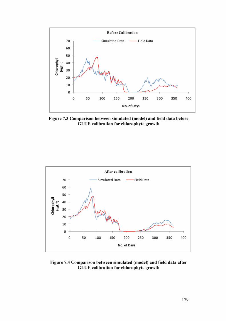
179


GLUE calibration for chlorophyte growth

Figure 7.4 Comparison between simulated (model) and field data after GLUE calibration for chlorophyte growth

0

10

20

30

40

50

60

70

0 50 100 150 200 250 300 350 400

Chloroph

yll

(ugL

-‐1)

No. of Days

Before Calibration

Simulated Data Field Data

0

10

20

30

40

50

60

70

0 50 100 150 200 250 300 350 400

Chloroph

yll

(ugL

-‐1)

No. of Days

After calibration

Simulated Data Field Data

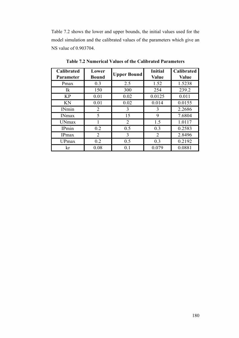
180

Table 7.2 shows the lower and upper bounds, the initial values used for the

model simulation and the calibrated values of the parameters which give an

NS value of 0.903704.

Table 7.2 Numerical Values of the Calibrated Parameters

Calibrated Parameter

Lower Bound Upper Bound

Initial Value

Calibrated Value

Pmax 0.3 2.5 1.52 1.5238Ik 150 300 254 239.2KP 0.01 0.02 0.0125 0.011KN 0.01 0.02 0.014 0.0155INmin 2 3 3 2.2686INmax 5 15 9 7.6804UNmax 1 2 1.5 1.0117IPmin 0.2 0.5 0.3 0.2583IPmax 2 3 2 2.8496UPmax 0.2 0.5 0.3 0.2192kr 0.08 0.1 0.079 0.0881

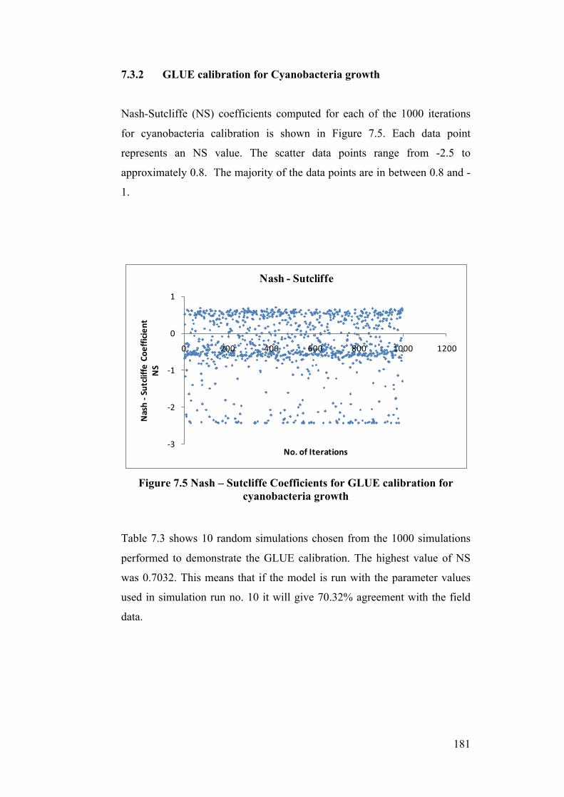
181

7.3.2 GLUE calibration for Cyanobacteria growth

Nash-Sutcliffe (NS) coefficients computed for each of the 1000 iterations

for cyanobacteria calibration is shown in Figure 7.5. Each data point

represents an NS value. The scatter data points range from -2.5 to

approximately 0.8. The majority of the data points are in between 0.8 and -

1.

Figure 7.5 Nash – Sutcliffe Coefficients for GLUE calibration for

cyanobacteria growth

Table 7.3 shows 10 random simulations chosen from the 1000 simulations

performed to demonstrate the GLUE calibration. The highest value of NS

was 0.7032. This means that if the model is run with the parameter values

used in simulation run no. 10 it will give 70.32% agreement with the field

data.

-‐3

-‐2

-‐1

0

1

0 200 400 600 800 1000 1200

Nash -‐Sutcliffe

Coe

fficie

ntNS

No. of Iterations

Nash - Sutcliffe

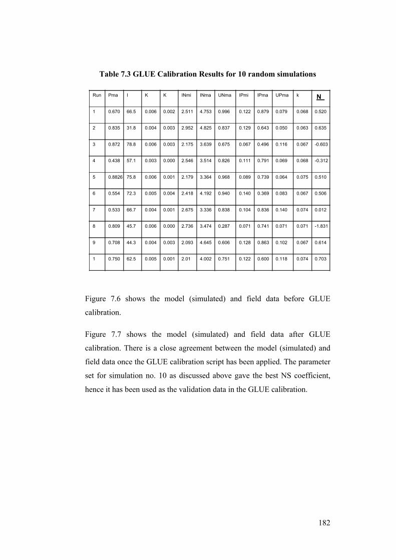
182

Table 7.3 GLUE Calibration Results for 10 random simulations

Figure 7.6 shows the model (simulated) and field data before GLUE

calibration.

Figure 7.7 shows the model (simulated) and field data after GLUE

calibration. There is a close agreement between the model (simulated) and

field data once the GLUE calibration script has been applied. The parameter

set for simulation no. 10 as discussed above gave the best NS coefficient,

hence it has been used as the validation data in the GLUE calibration.

Run

s Pma

x I

K K

P K

N INmi

n INma

x UNma

x IPmi

n IPma

x UPma

x k

r N

S 1 0.670

2 66.5

7 0.006

0 0.002

9 2.511

7 4.753

2 0.996

3 0.122

6 0.879

9 0.079

7 0.068

5 0.520

9 2 0.835

3 31.8

0 0.004

9 0.003

9 2.952

4 4.825

0 0.837

7 0.129

4 0.643

2 0.050

0 0.063

1 0.635

9 3 0.872

9 78.8

1 0.006

5 0.003

7 2.175

9 3.639

5 0.675

0 0.067

4 0.496

9 0.116

5 0.067

9 - 0.603

6

4 0.438

6 57.1

6 0.003

9 0.000

9 2.546

4 3.514

9 0.826

1 0.111

0 0.791

4 0.069

6 0.068

7 - 0.312

3 5 0.8826

75.8

7 0.006

7 0.001

0 2.179

0 3.364

5 0.968

0 0.089

4 0.739

9 0.064

2 0.075

9 0.510

1 6 0.554

3 72.3

4 0.005

7 0.004

7 2.418

3 4.192

5 0.940

2 0.140

4 0.369

8 0.083

1 0.067

2 0.506

8 7 0.533

5 66.7

4 0.004

5 0.001

6 2.675

7 3.336

6 0.838

1 0.104

8 0.836

2 0.140

7 0.074

5 0.012

8 8 0.809

2 45.7

2 0.006

1 0.000

7 2.736

2 3.474

3 0.287

9 0.071

1 0.741

9 0.071

5 0.071

1 - 1.831

9 9 0.708

1 44.3

6 0.004

9 0.003

2 2.093

1 4.645

3 0.606

9 0.128

3 0.863

9 0.102

4 0.067

8 0.614

5 1

0 0.750

0 62.5

0 0.005

2 0.001

0 2.01

5 4.002

0 0.751

1 0.122

4 0.600

0 0.118

3 0.074

0 0.703

2

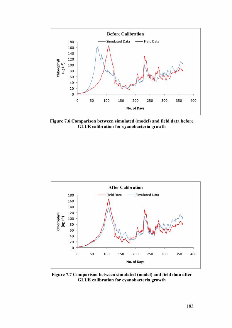
183


GLUE calibration for cyanobacteria growth


GLUE calibration for cyanobacteria growth

020406080100120140160180

0 50 100 150 200 250 300 350 400

Chloroph

yll

(ug L-‐1 )

No. of Days

Before CalibrationSimulated Data Field Data

020406080100120140160180

0 50 100 150 200 250 300 350 400

Chloroph

yll

(ug L-‐1 )

No. of Days

After CalibrationField Data Simulated Data

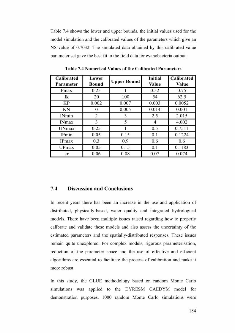
184

Table 7.4 shows the lower and upper bounds, the initial values used for the

model simulation and the calibrated values of the parameters which give an

NS value of 0.7032. The simulated data obtained by this calibrated value

parameter set gave the best fit to the field data for cyanobacteria output.

Table 7.4 Numerical Values of the Calibrated Parameters

7.4 Discussion and Conclusions

In recent years there has been an increase in the use and application of

distributed, physically-based, water quality and integrated hydrological

models. There have been multiple issues raised regarding how to properly

calibrate and validate these models and also assess the uncertainty of the

estimated parameters and the spatially-distributed responses. These issues

remain quite unexplored. For complex models, rigorous parameterisation,

reduction of the parameter space and the use of effective and efficient

algorithms are essential to facilitate the process of calibration and make it

more robust.

In this study, the GLUE methodology based on random Monte Carlo

simulations was applied to the DYRESM CAEDYM model for

demonstration purposes. 1000 random Monte Carlo simulations were

Calibrated Parameter

Lower Bound Upper Bound

Initial Value

Calibrated Value

Pmax 0.25 1 0.52 0.75Ik 20 100 54 62.5KP 0.002 0.007 0.003 0.0052KN 0 0.005 0.014 0.001INmin 2 3 2.5 2.015INmax 3 5 4 4.002UNmax 0.25 1 0.5 0.7511IPmin 0.05 0.15 0.1 0.1224IPmax 0.3 0.9 0.6 0.6UPmax 0.05 0.15 0.1 0.1183kr 0.06 0.08 0.07 0.074

185

conducted using parameters selected from the sensitivity analysis study in

Chapter 6. Large number of simulations would have required increased

computational times which would have not have been feasible and within

the time frame of this research work. After each simulation, the Nash-

Sutcliffe (NS) coefficient was computed. Multiple adjustments were made

to the data files in CAEDYM to be able to read the data for the

corresponding parameter. Program codes were written in FORTRAN 90 to

execute the above procedure. Pseudo field data was generated to run the

GLUE calibration module.

Chlorophyte and cyanobacteria growth output was used to demonstrate

GLUE calibration. Out of the 1000 iterations, the best NS coefficient

obtained was 0.9037 and 0.7032 for chlorophyte and cyanobacteria

respectively. Figure 7.4 and Figure 7.7 show a close agreement between the

simulated and pseudo field data after executing the GLUE calibration

program, which proves that the program can be used for model validation

purposes in future. This is definitely an improvement in the field of model

validation for DYRESM CAEDYM, as opposed to the previous “trial and

error” method which was time consuming and inaccurate. The complexity

of parameter interactions and their influence on the output in DYRESM

CAEDYM is enormous (as a combination of parameters has a profound

effect on a single output), and obtaining a “near perfect” parameter

combination using manual adjustments is extremely difficult. Thus the

calibration program as demonstrated in this chapter assists in overcoming

these challenges.

However, as much as the calibration process is automated, the user’s insight

and knowledge cannot be replaced. For example, while using the GLUE

method to calibrate DYRESM CAEDYM, the user decides which

parameters to calibrate by understanding which have the most influence on

model predictions for a specific case, through preliminary simulations and

acquired experience. Understanding the driving forces that work in each

simulation is critical to avoid the problem of over parameterisation and

unnecessary lengthy computational times.

186

7.5 Further Work

There is reasonable scope for further work to be conducted in this field.

• Simulations should be run with a larger number of iterations

(~100000) to obtain a better fit with the field data. Larger number of

simulations would require increased computing times, but would

provide a better accuracy in calibrating parameters. The chances of

obtaining a parameter set closest to the field data would be increased

significantly if the number of iterations are increased.

• Other outputs from the model e.g., nutrient data should also be

calibrated using the above procedure for effective model validation.

The main program is capable of including more parameters for

calibration. Additional parameters would require increased

computing times but would provide more accuracy in model outputs.

187

8 Summary and Conclusions

8.1 General Discussions and Conclusions

The aim of this PhD research was to develop a mathematical model for a

commercial scale IBS based on the suitability of DYRESM CAEDYM as a

modelling package and to use the results obtained from this modelling

exercise for deciding the required control and management of the IBS.

The objectives of this research were to

1. Obtain chemical parameters for piggery effluent from a two stage

anaerobic digestion system to serve as an input to the aquaculture

model.

2. Use numerical modelling techniques to test the suitability of

DYRESM CAEDYM as a modelling tool to model a commercial

scale IBS with a depth of 1 m.

3. Conduct a sensitivity analysis on the model parameters.

4. Use computer programming techniques to enable an automated

parameter estimation and calibration of the mathematical model.

8.2 Summary of the Research Results

This thesis has demonstrated the suitability of developing a mathematical

model for the IBS utilising piggery effluent as the nutrient source and has

provided results in the following key areas:

8.2.1 Laboratory Experiments and Development of Anaerobic

Digestion Model

The set up, installation and commissioning of the pilot scale two stage

anaerobic digestion system was conducted for a period of approximately 12

months. The main objective of this two-stage anaerobic digestion system

(comprising of a thermophilic system followed by a mesophilic digestion

system) was to conduct experiments to maximise throughput of raw piggery

effluent, whilst maintaining a high biogas generation. The experiments were

188

conducted in stages, with each stage having different hydraulic retention

times (HRT). The thermophilic (acidogenic) stage had HRT of 6.7 days,

while the mesophilic (methanogenic) stage had HRT of 15 days. Data for

pH, total solids, volatile solids, soluble COD, TKN, TAN, soluble P, VFA,

biogas volume and % CH4 in biogas was collected regularly. The set up,

installation and experiments conducted with the pilot plant system provided

an opportunity to understand the kinetics of raw piggery effluent digestion,

which paved a way for the development of an anaerobic digestion model.

A pilot scale integrated aquaculture (mesocosm) facility was set up in an

indoor climate controlled environment utilising anaerobically digested

piggery effluent for the culture of microalgae, zooplankton and fish.

Experiments were conducted relating to bioconversion of microalgae using

digested piggery effluent. The working volume of the microalgae (Chlorella

spp.) culture was kept at 280L and 180L, and the nutrient concentration was

fixed at 30 mg/L/day. Cell density, pH, TAN and phosphorus measurements

were taken daily. These experiments provided a better understanding of the

nutrient interactions and biomass conversions between digested piggery

effluent and microalgae which proved valuable during the simulations of the

aquaculture model DYRESM CAEDYM.

Batch scale anaerobic digestion experiments were conducted in the

laboratory for the development of a mathematical model. These experiments

were conducted in a batch mode to understand the degradation of raw

piggery effluent over a period of time and to obtain nutrient parameters of

TAN, soluble P, COD and pH which were necessary inputs to DYRESM

CAEDYM.

Analysis of the raw data from the batch scale experiments showed that TAN

and P were not correlated to methane production as initially suspected. A

new approach to modelling the anaerobic digestion system was utilised

which involved separate microbial kinetics for TAN, P and methane

production. Data outputs proved that both TAN/ Soluble P and COD/ CH4

followed two different sets of processes which were not correlated.

189

Microbial equations were developed which were used to fit the batch data

using “minimisation of errors squared” technique. The methane model

developed was remarkably different to other published models. It was

observed that methanogenesis was not the rate limiting step. Methane

production was found to be proportional to COD reduction, while P and

TAN were observed not to be proportional to COD.

8.2.2 Modelling the Aquaculture Component of the IBS

DYRESM CAEDYM was chosen as the appropriate modelling tool to

model the aquaculture stages of the IBS, consisting of bioconversion stages

of algae, zooplankton and fish. The ponds in the IBS were designed for a

depth of 1.0 m.

Initial simulations did not prove to be successful as the source code for

DYRESM CAEDYM had been originally written to simulate deep water

bodies ( > 5 m). The source code for this software was obtained from Centre

for Water Research (CWR), University of Western Australia (UWA), Perth

and compiled using Intel Visual Fortran Compiler 10 on Microsoft Visual

Studio 2005. On executing the program in debug mode with multiple

breakpoints, the parameters which caused the program to crash at depths

<5m were identified. These parameters were

• AREA_HT_DELTA_Z

• COEFFS_TBL_DELTA_Z

• INTERP_DELTA_Z

• MIN_GRID_THICK

Lower values for these parameters were set and the program re-compiled.

The software was able to then successfully simulate IBS ponds of depth 1.0

m.

0.2 m3 day-1 of anaerobically digested piggery effluent was passed through

each of the stages of the IBS. There was an overall 99.99% reduction in

NH4 concentration in the system. Chlorophyte growth peaked to a maximum

of 90 µg (chl-a) L-1 in the algal pond 1 and 60 µg (chl-a) L-1 in algal pond 2

190

followed by a sharp decrease. Cyanobacteria dominated both the algal ponds

1 and 2 with a maximum concentration of 200 mg m-3 and 150 mg m-3

respectively. Freshwater diatoms did not have any significant growth in

either pond due to low availability of silicon. Zooplankton growth exhibited

short spikes of periodic growth followed by a rapid decline and peaked to a

maximum of 0.6 g C m-3. Fish growth varied over the entire simulation

period and reached a maximum value of 0.8 g C m-3. The results obtained

here were different to those that would have been expected of an IBS, as in

an IBS there is effective management and control mechanisms put in place

which prevent the dominance of cyanobacteria and facilitate the increased

bioconversion rates of phytoplankton, zooplankton and fish, while the

simulations conducted on the proposed commercial scale IBS did not have

any control mechanisms incorporated into the model. A comparison study

with the pilot plant lagoon system in France also showed phytoplankton

growth crashes in summer due to dominance of rotifers as this system also

did not have any control mechanisms. However the researchers at the site in

France discovered that incorporation of certain control strategies, such as,

injection of carbon dioxide and slight agitation (mixing) improved the algal

productivity. The comparative IBS examples sourced from sites in India and

France show that IBS has been successfully implemented in different parts

of the world comprising tools for better control and management of ponds.

The use of mixing (agitation) and aeration assist in mixing the ponds and the

effluent uniformly which minimises stratification in ponds and thus reduces

the growth of cyanobacteria, and in turn improves the growth of

phytoplankton, zooplankton and fish. The model DYRESM CAEDYM

could incorporate the use of mixers and aeration in the IBS ponds to

overcome the problems of algal crashes in summer.







191


compatible module design.

8.2.3 Sensitivity Analysis

A sensitivity analysis was conducted on selected parameters of the model.

These parameters were subject to minimum, maximum and mean values and

simulations were run with these values. For each simulation, the output was

observed with reference to changes in values of chlorophyll-a concentration.

Chlorophyll a growth was considered to be one of the most important

outputs for this research as it was well correlated with biomass production

in the proposed commercial scale. IBS Parameters for which chlorophyll-a

was highly sensitive were those that directly altered growth rates i.e.

maximum phytoplankton growth rate (Pmax), phytoplankton respiration

coefficient (kr) and phytoplankton temperature multiplier (vR), or indirectly

affect growth rates through their ability to utilize phosphorus ( IPmin and

UPmax) , nitrogen (INmin and UNmax) and light penetration properties (Ik).

8.2.4 Automated Parameter Estimation and Calibration

Parameter calibration for DYRESM CAEDYM has been a tedious and time

consuming process involving manual input of values for every simulation. A

“trial and error” process has been used in the past, which resulted in

unsatisfactory results for model validation.

A calibration program, written in FORTRAN 90, involving Bayesian Monte

Carlo method and GLUE was set up to enable automated parameter

calibration in DYRESM CAEDYM. Due to the unavailability of real time

field data, pseudo field data was generated with random values for this

calibration routine to function properly. The model was calibrated by

minimizing the phytoplankton growth output parameter (chlorophyll-a in

case of chlorophyte calibration and mg m-3 in case of cyanobacteria

calibration).

192

For demonstration purposes, chlorophyte and cyanobacteria growth were

calibrated using the GLUE methodology incorporated into DYRESM

CAEDYM. 1000 Monte Carlo simulations were run using selected

parameters whose range was obtained from literature. For chlorophyte

calibration, a particular set of parameters gave 90.37% agreement (NS value

of 0.9037) with the field data for chlorophyte calibration. For cyanobacteria

calibration, a different set of parameters gave 70.32% agreement (NS value

of 0.7032) with the field data for cyanobacteria calibration.

8.3 Summary

The results presented in this thesis describe the outputs from the anaerobic

digestion experiments, involving both the two-stage pilot and the batch scale

set up, the suitability of DYRESM CAEDYM to model the aquaculture

stages of the IBS and the auto calibration program using FORTRAN 90 to

automatically validate the DYRESM CAEDYM with field data. Validating

the suitability of modelling IBS ponds using DYRESM CAEDYM and the

auto calibration program has closed the gap identified in the literature

review.

8.4 Recommendations for further studies

The mathematical model developed for the aquaculture component of the

IBS using DYRESM CAEDYM as the mathematical modelling tool

represents qualitative data only. Data for validating this model was not

available to the researcher due to the commercial outdoor IBS facility not

being constructed within the stipulated time at Roseworthy, South Australia.

Once the outdoor ponds have been constructed, the IBS facility should be

run on a continuous basis for a period of couple of years and data should be

collected regularly. The data collected should be validated against the

proposed IBS aquaculture model and the automated calibration routine run

several times to minimize the error between the simulated and field data.

193

Further investigation needs to be done on the response of different outputs

e.g. cyanobacteria, freshwater diatoms, zooplankton, fish growth etc in a

effectively controlled and managed system with changes in the parameters

selected for this study and additional parameters as well. This is useful in

identifying the parameters which are most sensitive to a particular output.

However when the number of parameters increases along with a variety of

outputs to be assessed, a manual method of altering parameter values to

observe the change in output is time consuming and more of a “trial and

error” approach. Also this sensitivity study relies on using the minimum,

maximum and mean values of the parameters selected without observing

any changes in the intermediate values, i.e. observing any changes in the

output during incremental changes to the selected parameter.

The automated calibration routine should be tested against other model

outputs e.g. nutrients, temperature, pH, DO etc to enable it to be used for

calibrating different outputs as desired by the modeller. The number of

iterations should also be increased to a larger value (~>100000) to obtain a

better precision in the values of the parameters calibrated. However this is

something that the modeller needs to decide because a balance needs to be

maintained between data precision and extensive computational time.

In recent years there has been an increase in the use and application of

distributed physically-based, water quality and integrated hydrological

models with the increase in the demand for efficiently managing the

precious water resources. There have been multiple issues raised regarding

how to properly calibrate and validate these models and also assess the

uncertainty of the estimated parameters and the spatially-distributed

responses. These issues remain quite unexplored. For complex models,

rigorous parameterisation, reduction of the parameter space and the use of

effective and efficient algorithms are essential to facilitate the process of

calibration and make it more robust. To efficiently calibrate, validate and

use a mathematical model, an automated calibration method is required

which eliminates the conventional techniques of calibrating parameters of

the model with a “trial and error” approach and introduces a sophisticated

194

automated method which reduces the scope of computational errors and

provides more realistic outputs which are of valuable guidance to the

process engineers. Water recycling and re-use applications require an

effective method of management, optimisation and control of the process

parameters and system which can be accomplished by the use of a robust

mathematical model. The robust models come with proper calibration and

validation. This study delivers valuable information and innovative method

to calibrate and validate the use of model.

The use of automated calibration method has high applicability particularly

in the development of mathematical models for managing the performance

of wastewater recycling technology which is being highly sought by the

modern world in order to minimise the impact on diminishing precious

water resources. This calibration technique has also demonstrated that for a

complex aquaculture model like DYRESM CAEDYM where manually

validating the parameters is an unwieldy task, automatic calibration routine

using GLUE methodology is an effective way to validate the model which

reduces the risks of computational errors.

195

9 References

Ambler, J. W. (1986). "Effect of food quantity and quality on egg production of

Acartia tonsa Dana from East Lagoon, Galveston, Texas." Estuarine, Coastal and

Shelf Science 23(2): 183-196.

Andersen, J., J. C. Refsgaard, et al. (2001). "Distributed hydrological modelling of

the Senegal River Basin -- model construction and validation." Journal of

Hydrology 247(3-4): 200-214.

Andrews, J. F. (1969). "Dynamic model of the anaerobic digestion model." J.

Sanit. Engng. 1: 95 - 116.

Angelidaki, I., L. Ellegaard, et al. (1993). "A mathematical model for dynamic

simulation of anaerobic digestion of complex substrates: focussing on ammonia

inhibition." Biotechnology and Bioengineering 42: 159 - 166.

APHA, AWWA, et al. (1998). Standard Methods for the Examination of Water

and Wastewater. Washington DC, USA.

Appels, L., J. Lauwers, et al. (2011). "Anaerobic digestion in global bio-energy

production: Potential and research challenges." Renewable and Sustainable

Energy Reviews 15(9): 4295-4301.

Aronica, G., P. D. Bates, et al. (2002). "Assessing the uncertainty in distributed

model prediction using observed binary pattern information with GLUE."

Hydrological Processes 16: 2001 - 2016.

Aronica, G., B. Hankin, et al. (1998). "Uncertainty and equifinality in calibrating

distributed roughness coefficients in a flood propagation model with limited data."

Advances in Water Resources 22(4): 349-365.

196

Balistrieri, L. S., R. N. Tempel, et al. (2006). "Modeling spatial and temporal

variations in temperature and salinity during stratification and overturn in Dexter

Pit Lake, Tuscarora, Nevada, USA." Applied Geochemistry 21(7): 1184-1203.

Bergman, B., J. R. Gallon, et al. (1997). "N2 Fixation by non-heterocystous

cyanobacteria." FEMS Microbiology Reviews 19(3): 139-185.

Beven, K. (1993). "Prophecy, reality and uncertainty in distributed hydrological

modelling." Advances in Water Resources 16(1): 41-51.

Beven, K. and J. Freer (2001). "Equifinality, data assimilation, and uncertainty

estimation in mechanistic modelling of complex environmental systems using the

GLUE methodology." Journal of Hydrology 249(1-4): 11-29.

Beven, K. J. and A. Binley (1992). "The future of distributed models: model

calibration and uncertainty prediction." Hydrological Processes 6: 279 - 298.

Blasone, R.-S., J. A. Vrugt, et al. (2008). "Generalized likelihood uncertainty

estimation (GLUE) using adaptive Markov Chain Monte Carlo sampling."

Advances in Water Resources 31(4): 630-648.

Boon, P. I., S. E. Bunn, et al. (1994). "Consumption of cyanobacteria by

freshwater zooplankton: implications for the success of 'Top - down' control of

cyanobacterial blooms in Australia." Australian Journal of Marine and Freshwater

Research. 45(5): 875 - 887.

Boyle, D. P., H. V. Gupta, et al. (2000). "Towards improved calibration of

hydrological models: combining the strengths of manual and automatic methods."

Water Resources Research 36: 3663 - 3674.

Brix, H. and H. H. Scheirup (1989). "The use of aquatic macrophytes in water

pollution control." Ambio 18: 100 -107.

197

Bruce, L. C., D. Hamilton, et al. (2006). "A numerical simulation of the role of

zooplankton in C, N and P cycling in Lake Kinneret, Israel." Ecological

Modelling 193(3-4): 412-436.

Bryers, J. D. (1985). "Structured modelling of the anaerobic digestion of biomass

particulates." Biotechnology and Bioengineering. 27: 638 - 649.

Budiastuti, H. (2004). Intensification of Single Stage Continously Stirred Tank

Anaerobic Digestion Process using Carriers. School of Environmental Science.

Perth, Western Australia, Murdoch University.

Burger, D. F., D. P. Hamilton, et al. (2008). "Modelling the relative importance of

internal and external nutrient loads on water column nutrient concentrations and

phytoplankton biomass in a shallow polymictic lake." Ecological Modelling

211(3-4): 411-423.

Cameron, D. S., K. J. Beven, et al. (1999). "Flood frequency estimation by

continous simulation for a gauged upland catchment (with uncertainty)." Journal

of Hydrology 219: 169 - 187.

Carlotti, F., J. Giske, et al. (2000). 12 - Modeling zooplankton dynamics. ICES

Zooplankton Methodology Manual. H. Roger, W. Peter, L. J√ºrgenet al. London,

Academic Press: 571-667.

Chen, C., R. Ji, et al. (2002). "A model study of the coupled biological and

physical dynamics in Lake Michigan." Ecological Modelling 152(2-3): 145-168.

Chen, Y. R. (1983). "Kinetic analysis of anaerobic digestion of pig manure and its

design implications." Agricultural Wastes 8(2): 65-81.

Chen, Y. R. and A. G. Hashimoto (1978). "Kinetics of methane formation."

Biotechnology and Bioengineering Symposium. 8: 269.

198

Choi, H. T. and K. Beven (2007). "Multi-period and multi-criteria model

conditioning to reduce prediction uncertainty in an application of TOPMODEL

within the GLUE framework." Journal of Hydrology 332(3-4): 316-336.

Christiaens, K. and J. Feyen (2001). "Analysis of uncertainties associated with

different methods to determine soil hydraulic properties and their propagation in

the distributed hydrological MIKE SHE model." Journal of Hydrology 246(1-4):

63-81.

Costello, D. J., P. F. Greenfield, et al. (1991a). "Dynamic modelling of a single -

stage high - rate anaerobic reactor - I. Model derivation." Water Resources 25:

847 - 858.

Costello, D. J., P. F. Greenfield, et al. (1991b). "Dynamic modelling of a single -

stage high - rate anaerobic reactor - II. Model verification." Water Resources 25:

859 - 871.

Crips, S. and M. S. Kumar (2003). Environmental and other impact of

aquaculture. In Aquaculture: Farming fish and Shellfish. L. J. S. a. S. P.C.,

Blackwell Publications, U.K.

Curtis, T. P., D.D. Mara, S.A. Silva (1992). "The effect of sunlight on faecal

coliforms in ponds: Implications for research and design." Water Science and

Technology 26(78): 1729-1738.

Cyr, H. and M. L. Pace (1992). "Grazing by zooplankton and its relationship to

community structure." Canadian Journal of Fisheries and Aquatic Sciences. 49(7):

1455 - 1465.

De Melo, R., R. France, et al. (1992). "Biomanipulation: hit or myth?" Limnology

Oceanography 37: 192 - 207.

Di Termini, I., A. Prassone, et al. (2011). "On the nitrogen and phosphorus

removal in algal photobioreactors." Ecological Engineering 37(6): 976-980.

199

Di Toro, D. M., D. J. O' Connor, et al. (1971). "A Dynamic Model for the

Phytoplankton Population in the Sacramento San Joaquin Delta." Adv. Chem. Ser.

106: 131 - 180.

Donoso-Bravo, A., J. Mailier, et al. (2011). "Model selection, identification and

validation in anaerobic digestion: A review." Water Research 45(17): 5347-5364.

Durbin, A. G. and E. G. Durbin (1992). "Seasonal change in size frequency

distribution and estimated age in the marine copepod Acartia hudsonica during a

winter - spring diatom bloom in the Narragansett Bay. ." Limnology

Oceanography 37: 379 - 392.

Eastman, J. A. and J. F. Ferguson (1981). "Solubilization of Particulate Organic

Carbon during the Acid Phase of Anaerobic Digestion." Journal of the Water

Pollution Control Federation 53: 352 - 366.

Edwards, P. and R. S. V. Pullin (1990). General Discussion on wastewater - fed

aquaculture. . Proceedings of the International Seminar on Wastewater

Reclamation and Reuse for Aquaculture, Calcutta, India.

Egge, J. K. and D. L. Aksnes (1992). "Silicate as regulating nutrient in

phytoplankton competition." Marine Ecology Progress Series 83: 281-289.

Emerson, K. e. a. (1975). "Aqueous Ammonia Equilibrium Calculations: Effect of

pH and temperature. ." J. Fish. Res. Board Can. 32(12).

Engeland, K., I. Braud, et al. (2006). "Multi-objective regional modelling."

Journal of Hydrology 327(3-4): 339-351.

Feyen, L., K. Beven, et al. (2001). "Stochastic capture zone delineation within the

generalized likelihood uncertainty estimation methodology; conditioning on head

observations." Water Resources Research 37(3): 625 - 638.

200

Fiore, M. d. F. t., B. A. Neilan, et al. (2005). "Characterization of nitrogen-fixing

cyanobacteria in the Brazilian Amazon floodplain." Water Research 39(20): 5017-

5026.

Fisher, H. B., E. G. List, et al. (1979). Mixing in Inland and Coastal Waters.,

Academic Press.

Flachowsky, G. and A. Hennig (1990). "Composition and digestibility of

untreated and chemically treated animal excreta for ruminants--A review."

Biological Wastes 31(1): 17-36.

Fragoso Jr, C. R., D. M. L. M. Marques, et al. (2008). "Modelling spatial

heterogeneity of phytoplankton in Lake Mangueira, a large shallow subtropical

lake in South Brazil." Ecological Modelling 219(1-2): 125-137.

Freer, J., K. J. Beven, et al. (1996). "Bayesian estimation of uncertainty in runoff

prediction and the value of data: an application of the GLUE approach." Water

Resources Research 32(7): 2161 - 2173.

Freer, J. E., H. McMillan, et al. (2004). "Constraining dynamic TOPMODEL

responses for imprecise water table information using fuzzy rule based

performance measures." Journal of Hydrology 291(3-4): 254-277.

Freund, J. A., S. Mieruch, et al. (2006). "Bloom dynamics in a seasonally forced

phytoplankton‚Äìzooplankton model: Trigger mechanisms and timing effects."

Ecological Complexity 3(2): 129-139.

Frost, B. W. (1972). "Effects of size and concentration of food particles on the

feeding behaviour of the marine planktonic copepod Calanus pacificus. ."

Limnology Oceanography. 17(6): 805 - 815.

Gal, G., J. Imberger, et al. (2003). "Simulating the thermal dynamics of Lake

Kinneret." Ecological Modelling 162(1-2): 69-86.

201

Gamble, J. C. (1978). "Copepod grazing during a declining spring phytoplankton

bloom in the northern North Sea. ." Marine Biology. 49: 303 - 315.

Georgakakos, K. P., D.-J. Seo, et al. (2004). "Towards the characterization of

streamflow simulation uncertainty through multimodel ensembles." Journal of

Hydrology 298(1-4): 222-241.

Gilbert, P. M. (1998). "Interactions of top - down and bottom - up control in

planktonic nitrogen cycling." Hydrobiologia 491: 91 - 100.

Gopakumar, K., S. Ayyappan, et al. (2000). Present Status of Integrated Fish

Farming in India and Wastewater Treatment Through Aquaculture Proceedings of

the National Workshop on Wastewater Treatment and Integrated Aquaculture.

Adelaide, South Australian Research & Development Institute (SARDI). 22 - 37.

Graef, S. P. and J. F. Andrews (1974). "Stability and control of Anaerobic

Digestion." Journal WPCF 46: 667 - 682.

Griffin, S. L., M. Herzfeld, et al. (2001). "Modelling the impact of zooplankton

grazing on phytoplankton biomass during a dinoflagellate bloom in the Swan

River Estuary, Western Australia." Ecological Engineering 16(3): 373-394.

Griffiths, F. B. and J. Caperon (1979). "Description and use of an improved

method for determining estuarine zooplankton grazing rates on phytoplankton. ."

Marine Biology 54: 301 - 309.

Gupta, H. V., S. A. Sorooshian, et al. (1998). "Toward improved calibration of

hydrologic models:multiple and noncommensurable measures of information."

Water Resources Research 34: 751 - 763.

Guven, B. and A. Howard (2006). "Modelling the growth and movement of

cyanobacteria in river systems." Science of The Total Environment 368(2-3): 898-

908.

202

H√•kanson, L. and V. V. Boulion (2003). "Modelling production and biomasses

of herbivorous and predatory zooplankton in lakes." Ecological Modelling 161(1-

2): 1-33.

H√•kanson, L., A. C. Bryhn, et al. (2007). "On the issue of limiting nutrient and

predictions of cyanobacteria in aquatic systems." Science of The Total

Environment 379(1): 89-108.

Håkanson, L. and V. V. Boulion (2003). "Modelling production and biomasses of

herbivorous and predatory zooplankton in lakes." Ecological Modelling 161(1-2):

1-33.

Hamilton, D. P., G. Schladow, et al. (1995). "Controlling the indirect effects of

flow diversions on water quality in an Australian reservoir." Environment

International 21(5): 583-590.

Hamilton, D. P. and S. G. Schladow (1997). "Prediction of water quality in lakes

and reservoirs. Part I -- Model description." Ecological Modelling 96(1-3): 91-

110.

Harper, S. R. and F. G. Pohland (1986). "Recent Development in Hydrogen

Measurement during Anaerobic Biological Wastewater Treatment."

Biotechnology and Bioengineering 28: 585 - 602.

Harris, G. P. (1986). Phytoplankton Ecology - Structure, Function and

Fluctuation. London, Chapman and Hall.

Havens, K. E., R. T. James, et al. (2003). "N:P ratios, light limitation, and

cyanobacterial dominance in a subtropical lake impacted by non-point source

nutrient pollution." Environmental Pollution 122(3): 379-390.

Heidari, A., B. Saghafian, et al. (2006). "Assessment of flood forecasting lead

time based on generalized likelihood uncertainty estimation." Stochastic

Environmental Research and Risk Assessment 20(5): 363 - 380.

203

Henriksen, H. J., L. Troldborg, et al. (2003). "Methodology for construction,

calibration and validation of a national hydrological model for Denmark." Journal

of Hydrology 280(1-4): 52-71.

Hense, I. and A. Beckmann (2006). "Towards a model of cyanobacteria life

cycle‚Äîeffects of growing and resting stages on bloom formation of N2-fixing

species." Ecological Modelling 195(3-4): 205-218.

Hense, I. and H. Burchard (2010). "Modelling cyanobacteria in shallow coastal

seas." Ecological Modelling 221(2): 238-244.

Hill, D. T. (1982). "A comprehensive dynamic model for animal waste

methanogenesis." Transactions of the ASAF 25: 1374 - 1380.

Hill, D. T. and C. L. Barth (1977). "A dynamic model for simulation of animal

waste digestion." Journal WPCF 10: 2129 - 2143.

Hipsey, M. R., J. R. Romero, et al. (2006). Computational Aquatic Ecosystem

Dynamics Model v2.3 Science Manual, Centre for Water Research, University of

Western Australia, Australia.

Hodges, B. and C. Dallimore (2001). Estuary and Lake Computer Model,

ELCOM, Science Manual, code version 1.5.0, Centre for Water Research,

University of Western Australia.

Hodgkin, E. P. and R. J. Rippingale (1971). "Interspecies conflict in estuarine

copepods." Limnology Oceanography 16: 573 - 576.

Hongping, P. and M. Jianyi (2002). "Study on the algal dynamic model for West

Lake, Hangzhou." Ecological Modelling 148(1): 67-77.

204

Hornberger, G. M. and R. C. Spear (1981). "An approach to the preliminary

analysis of environmental systems." Journal of Environmental Management 12: 7

- 18.

Huang, A. A. (1975). "Enzymatic Hydrolysis of Cellulose to Sugar."

Biotechnology and Bioengineering Symposium. 5: 245 - 252.

Hudson, J. J. and W. D. Taylor (1996). "Measuring regeneration of dissolved

phosphorus in planktonic communities." Limnol. Oceanogr. 41: 1560 - 1565.

Hudson, J. J., W. D. Taylor, et al. (1999). "Planktonic nutrient regeneration and

cycling efficiency in temperate lakes." Nature 400: 659 - 661.

Hunt, R. J. and V. F. Matveev (2005). "The effects of nutrients and zooplankton

community structure on phytoplankton growth in a subtropical Australian

reservoir: An enclosure study." Limnologica - Ecology and Management of Inland

Waters 35(1-2): 90-101.

Imberger, J. (1981). "The influence of stream salinity on reservoir water quality."

Agricultural Water Management 4(1-3): 255-273.

Imberger, J., J. C. Patterson, et al. (1978). "Dynamics of Reservoirs of Medium

Size." Journal of Hydrology, Division, ASCE 104(725 - 743).

Imerito, A. (2007). Dynamic Reservoir Simulation Model v4.0 Science Manual,

Centre for Water Research, University of Western Australia, Australia.

Islam, M. S. e. a. (1996). "Faecal contamination of a fish culture farm where

duckweed grown in hospital wastewater are used as fish feed." Proceedings of the

5th Annual Scientific Conference, ASCON, Dhaka, Bangladesh: 49.

Jefferson T, T. (2010). "Zooplankton community grazing impact on a bloom of

Alexandrium fundyense in the Gulf of Maine." Harmful Algae 9(6): 578-589.

205

Ji, R., C. Chen, et al. (2002). "Influences of suspended sediments on the

ecosystem in Lake Michigan: a 3-D coupled bio-physical modeling experiment."

Ecological Modelling 152(2-3): 169-190.

Jonathan P, Z. (2011). "Nitrogen fixation by marine cyanobacteria." Trends in

Microbiology 19(4): 162-173.

Jørgensen, S. E. (1995). "State of the art of ecological modelling in limnology."


Jørgensen, S. E., L. A. Jørgensen, et al. (1981). "Parameter estimation in

eutrophication modelling." Ecological Modelling 13(1-2): 111-129.

Jørgensen, S. E., L. Kamp-Nielsen, et al. (1975). "A submodel for anaerobic mud-

water exchange of phosphate." Ecological Modelling 1(2): 133-146.

Jørgensen, S. E., L. Kamp-Nielsen, et al. (1986). "Examination of the generality

of eutrophication models." Ecological Modelling 32(4): 251-266.

Jørgensen, S. E., H. Mejer, et al. (1978). "Examination of a lake model."


Kardinaal, W. E. A. and P. M. Visser (2005). "Dynamics of Cyanobacterial

Toxins: Sources of Variability in Microcystin Concentrations. ." Harmful

Cyanobacteria.

Kleinstreuer, C. and T. Powegha (1982). "Dynamic simulator for anaerobic

digestion process." Biotechnology and Bioengineering. 24: 1941 - 1951.

Klepper, O., H. Scholten, et al. (1991). "Predicition uncertainty in an ecological

model of the Oosterchelde Estuary." Journal of Forecasting 10: 191 - 209.

206

Kranert M., H. K. (2000). Anaerobic Digestion of Organic Wastes - Process

Parameters and Balances in Practice. Material Flow Analysis of Integrated

Biosystems.

Krebs, C. J. (1985). Ecology: The Experimental Analysis of Distribution and

Abundance. New York, Harper & Row.

Krivtsov, V., C. Goldspink, et al. (2001). "Expansion of the model [`]Rostherne'

for fish and zooplankton: role of top-down effects in modifying the prevailing

pattern of ecosystem functioning." Ecological Modelling 138(1-3): 153-171.

Kuczera, G. and E. Parent (1998). "Monte Carlo assessment of parameter

uncertainty in conceptual catchment models: the Metropolis algorithm." Journal of

Hydrology 211(1-4): 69-85.

Kumar, M. S. (2002). Integrated Farming for Sustainable Primary Industry:

“Water and Nutrient Recycling through Integrated Aquaculture” Proceedings of

the Infom 2000 National workshop on Integrated Food Production and Resource

management. “Integrated biosystem for sustainable Development”. W. a. Pillai-

McGrarry: 51 - 62.

Kumar, M. S. and S. Crips (2012). Environmental and Other Impact of

Aquaculture, Lucas, J.S. and Southgate P.C. Blackwell Publications, UK.

Kumar, M. S. and M. Sierp (2003). Integrated Wastewater Treatment and

Aquaculture Production. Adelaide, Rural Industries Research and Development

Corporation: 1 - 62.

Lamb, R., K. Beven, et al. (1998). "Use of spatially distributed water table

observations to constrain uncertainty in a rainfall-runoff model." Advances in

Water Resources 22(4): 305-317.

207

Lampert, W. and B. E. Taylor (1985). "Zooplankton grazing in a eutrophic lake:

implications of diel vertical migration." Ecology. 66: 68 - 82.

Le Hyaric, R., J.-P. Canler, et al. (2010). "Pilot-scale anaerobic digestion of

screenings from wastewater treatment plants." Bioresource Technology 101(23):

9006-9011.

Lee, M.-Y., C.-W. Suh, et al. (2009). "Variation of ADM1 by using temperature-

phased anaerobic digestion (TPAD) operation." Bioresource Technology 100(11):

2816-2822.

Lehman, J. T. (1980). "Release and cycling of nutrients between planktonic algae

and herbivores." Limnol. Oceanogr. 25: 620 - 632.

Levine, S. N., M. A. Borchardt, et al. (1999). "The Impact of Zooplankton

Grazing on Phytoplankton Species Composition and Biomass in Lake Champlain

(USA-Canada)." Journal of Great Lakes Research 25(1): 61-77.

Lewis, D. M., J. D. Brookes, et al. (2004). "Numerical Models for management of

Anabaena Circinalis." Journal of Applied Phycology 16: 457 - 468.

Lin, C. and K. Sato (1986). "Methanogenic Digestion Using Mixed Substrate of

Acetic, Propionic and Butyric Acids." Water Research 20(3): 385 - 394.

Lionard, M., F. Azemar, et al. (2005). "Grazing by meso- and microzooplankton

on phytoplankton in the upper reaches of the Schelde estuary." Estuarine, Coastal

and Shelf Science 64(4): 764-774.

Lunte, C. C. and C. Leucke (1990). "Trophic interactions of leptodora in Lake

Mendota." Limnol. Oceanogr. 35: 1091 - 1100.

Lyberatos, G. and I. V. Skiadas (1999). "Modelling of Anaerobic Digestion - A

Review." Global Nest: the Int. J 1(2): 63 - 76.

208

Mackas, D. and R. Bohrer (1976). "Flouresecence analysis of zooplankton gut

contents and investigation of diel feeding patterns. ." Journal of Experimental and

Marine Biology and Ecology. 25: 77 - 85.

Madsen, H. (2000). "Automatic calibration of a conceptual rainfall-runoff model

using multiple objectives." Journal of Hydrology 235(3-4): 276-288.

Madsen, H. (2003). "Parameter estimation in distributed hydrological catchment

modelling using automatic calibration with multiple objectives." Advances in

Water Resources 26(2): 205-216.

Madsen, M., J. B. Holm-Nielsen, et al. (2011). "Monitoring of anaerobic digestion

processes: A review perspective." Renewable and Sustainable Energy Reviews

15(6): 3141-3155.

Mansson, T., Foo, E.L. (1998). Swedish efforts in integrating bio-fuels as

alternative fuels for transportation in buses, lorries and cars. Proceedings of the

Internet Conference on Integrated Biosystems.

Mantovan, P. and E. Todini (2006). "Hydrological forecasting uncertainty

assessment: Incoherence of the GLUE methodology." Journal of Hydrology 330(1

- 2): 368 - 381.

Marino, R. W. and R. Howarth (2009). Nitrogen Fixation. Encyclopedia of Inland

Waters. E. L. Editor-in-Chief:¬†¬†Gene. Oxford, Academic Press: 65-72.

Martin, J. H. (1970). "Phytoplankton - zooplankton relationships in Narragansett

Bay. 4. The seasonal importance of grazing. ." Limnology Oceanography. 15: 413

- 418.

Matsuoka, Y., T. Goda, et al. (1986). "An eutrophication model of Lake

Kasumigaura." Ecological Modelling 31(1-4): 201-219.

209

McAllister, C. D. (1971). Some aspects of nocturnal and continuous grazing by

planktonic herbivores in relation to production studies. . Fisheries Research Board

of Canada.

McInerney, M. and M. Bryant (1981). "Basic Principles of Bioconversions in

Anaerobic Digestion of Methanogenesis." Biomass Conversion Processes for

Energy and Fuels: 227 - 296.

McInerney, M. J. and P. Beaty (1988). "Anaerobic Community Structure from a

Non Equilibrium Thermodynamic Perspective." Canadian Journal of

Microbiology 34: 487 - 493.

McMichael, C. E., A. S. Hope, et al. (2006). "Distributed hydrological modelling

in California semi - arid shrublands: MIKE SHE model calibration and

uncertainty estimation." Journal of Hydrology 317(3 - 4): 307 - 324.

Mertens, J., H. Madsen, et al. (2004). "Including prior information in the

estimation of effective soil parameters in unsaturated zone modelling." Journal of

Hydrology 294(4): 251-269.

Mitra, A. and K. J. Flynn (2006). "Accounting for variation in prey selectivity by

zooplankton." Ecological Modelling 199(1): 82-92.

Miyanaga, Y. (1986). "Modelling of stratified flow and eutrophication in

reservoirs." Ecological Modelling 31(1-4): 133-144.

Moletta, R., D. Verrier, et al. (1986). "Dynamic modelling of anaerobic

digestion." Water Research 20(4): 427-434.

Molina Grima, E., F. G. A. Fernández, et al. (1999). "Photobioreactors: light

regime, mass transfer, and scaleup." Journal of Biotechnology 70(1-3): 231-247.

210

Montanari, A. (2005). "Large sample behaviours of the generalized likelihood

uncertainty estimation (GLUE) in assessing the uncertainty of rainfall - runoff

simulations." Water Resources Research 41(W08406).

Moradkhani, H., K.-L. Hsu, et al. (2005). "Uncertainty assessment of hydrologic

model states and parameters; sequential data assimilation using the particle filter."

Water Resources Research 41(5): 1 - 17.

Mosey, F. E. (1983). "Mathematical modelling of the anaerobic digestion process:

regulatory mechanisms for the formation of short chain volatile acids from

glucose." Water Science Technology 15: 209 - 232.

Mueller, D. K. (1982). "Mass balance model for estimation of phosphorus

concentration in reservoirs." Water Resources Bulletin 18: 377 - 382.

Muleta, M. K. and J. W. Nicklow (2005). "Sensitivity and uncertainty analysis

coupled with automatic calibration for a distributed watershed model." Journal of

Hydrology 306(1-4): 127-145.

Mullin, M. M. and E. R. Brooks (1970). "The effect of concentration of food on

body size, cumulative ingestion, and rate of growth of the marine copepod

Calanus helgolandicus. ." Limnology Oceanography. 15: 748 - 755.

Mur, L. R., O. M. Skulberg, et al. (1999). "Cyanobacteria in the Environment."

Toxic Cyanobacteria in Water: A Guide to their Public Health Consequences,

Monitoring and Management.(World Health Organisation).

Myint, M. and N. Nirmalakhandan (2006). "Evaluation of First Order, Second

Order and Surface Limiting Reactions in Anaerobic Hydrolysis of Cattle

Manure." Environmental Engineering Science 23(6): 966 - 976.

Myint, M., N. Nirmalakhandan, et al. (2006). "Anaerobic Fementation of Cattle

Manure: Modelling of Hydrolysis and Acidogenesis." Water Research In Press,

Corrected Proof.

211

Nash, J. E. and J. V. Sutcliffe (1970). "River flow forecasting through conceptual

models part I -- A discussion of principles." Journal of Hydrology 10(3): 282-290.

Noike, T. and G. Endo (1985). "Characteristic of Carbohydrate Degradation and

the Rate Limiting Step in Anaerobic Digestion." Biotechnology and

Bioengineering 27(10): 1482 - 1489.

Osidele, O. O. and M. B. Beck (2004). "Food web modelling for investigating

ecosystem behaviour in large reservoirs of the south-eastern United States: lessons

from Lake Lanier, Georgia." Ecological Modelling 173(2-3): 129-158.

Ostfeld, A. and S. Salomons (2005). "A hybrid genetic--instance based learning

algorithm for CE-QUAL-W2 calibration." Journal of Hydrology 310(1-4): 122-

142.

Paerl, H. W., H. Xu, et al. (2011). "Controlling harmful cyanobacterial blooms in

a hyper-eutrophic lake (Lake Taihu, China): The need for a dual nutrient (N

& P) management strategy." Water Research 45(5): 1973-1983.

Pappenberger, F., K. Beven, et al. (2007). "Grasping the unavoidable subjectivity

in calibration of flood inundation models: A vulnerability weighted approach."

Journal of Hydrology 333(2-4): 275-287.

Pappenberger, F., K. Beven, et al. (2005). "Uncertainty in the calibration of

effective roughness parameters in HEC-RAS using inundation and downstream

level observations." Journal of Hydrology 302(1-4): 46-69.

Parker, W. J. (2005). "Application of the ADM1 model to advanced anaerobic

digestion." Bioresource Technology 96(16): 1832-1842.

Pearson, H. W., D.D. Mara, L.R. Cawley, H.M. Arridge, S.A. Silva (1996). "The

performance of an innovative tropical experiment waste stabilization pond system

operating at high organic loadings." Water Science and Technology 33(7): 63-73.

212

Pearson, H. W., D.D. Mara, S.W. Mills, D.J. Smallman (1987). "Physico-

chemical parameters influencing faecal bacterial survival in waste stabilization

ponds." Water Science and Technology 11(12): 145-152.

Peterson, W. T., S. Painting, et al. (1990). "Diel variation in gut pigment content,

diel vertical migration and estimates of grazing impact for copepods in the

southern Benguella upwelling region in October 1987." Journal of Plankton

Research. 12: 259 - 281.

Poulsen, O. M. and L. W. Peterson (1985). "A Standard Formula for the

Determination of the Initial Rate of Hydrolysis of Carboxymethylcellulase."

Biotechnology and Bioengineering 27: 409 - 414.

Pullammanappallil, P., D. P. Chynoweth, et al. (2001). "Stable performance of

anaerobic digestion in the presence of high concentration of propionic acid."

Bioresource Technology 78: 165 - 169.

Pullammanappallil, P., J. M. Owens, et al. (1991). "Dynamic model for

conventionally mixed anaerobic digestion reactors." AIChE Annual

Meeting(277c): 43 - 53.

Rajagopal, R., P. Rousseau, et al. (2011). "Combined anaerobic and activated

sludge anoxic/oxic treatment for piggery wastewater." Bioresource Technology

102(3): 2185-2192.

Ramirez, I., E. I. P. Volcke, et al. (2009). "Modeling microbial diversity in

anaerobic digestion through an extended ADM1 model." Water Research 43(11):

2787-2800.

Ratto, M., S. Tarantola, et al. (2001). "Sensitivity analysis in model calibration:

GSA-GLUE approach." Computer Physics Communications 136(3): 212-224.

213

Ray, S., L. Berec, et al. (2001). "Optimization of exergy and implications of body

sizes of phytoplankton and zooplankton in an aquatic ecosystem model."

Ecological Modelling 140(3): 219-234.

Reeve, M. R. and M. A. Walter (1977). "Observations on the existence of lower

threshold and upper critical food concentrations for the copepod Acartia tonsa

Dana." Journal of Experimental and Marine Biology and Ecology. 29: 211 - 221.

Refsgaard, J. C. (1997). "Parameterisation, calibration and validation of

distributed hydrological models." Journal of Hydrology 198(1-4): 69-97.

Riley, M. J. and H. G. Stefan (1988). "Minlake: A dynamic lake water quality

simulation model." Ecological Modelling 43(3-4): 155-182.

Rippingale, R. J. (1994). "A calanoid copepod Gladioferans imparipes, holding

onto surfaces." Hydrobiology. 292/293: 351 - 360.

Rippingale, R. J. and E. P. Hodgkin (1974a). "Predation effects on the distribution

of a copepod." Australian Journal of Marine and Freshwater Research. 25: 81 - 91.

Rippingale, R. J. and E. P. Hodgkin (1974b). "Population growth of a copepod

Gladioferens imparipes Thomson." Australian Journal of Marine and Freshwater

Research. 25: 351 - 360.

Rippingale, R. J. and E. P. Hodgkin (1977). "Food availability and salinity

tolerance in a brackish water copepod. ." Australian Journal of Marine and

Freshwater Research. 28: 1 - 7.

Robson, B. J. and D. P. Hamilton (2004). "Three-dimensional modelling of a

Microcystis bloom event in the Swan River estuary, Western Australia."


214

Romero, J. R., J. P. Antenucci, et al. (2004). "One- and three-dimensional

biogeochemical simulations of two differing reservoirs." Ecological Modelling

174(1-2): 143-160.

Romli, M. (1993). "Modelling and Verification of a Two Stage Anaerobic

Wastewater Treatment System." Chemical Engineering.

Rozzi, A. and S. Merlini (1985). "Development of a Four Population Model of the

Anaerobic Degradation of Carbohydrate." Environmental Technology Letters 6:

10 - 19.

Rukhovets, L. A., G. P. Astrakhantsev, et al. (2003). "Development of Lake

Ladoga ecosystem models: modeling of the phytoplankton succession in the

eutrophication process. I." Ecological Modelling 165(1): 49-77.

Salomoni, C., A. Caputo, et al. (2011). "Enhanced methane production in a two-

phase anaerobic digestion plant, after CO2 capture and addition to organic

wastes." Bioresource Technology 102(11): 6443-6448.

Santos, M. a. d. l. Å. M. n., J. Å. S. L√≥pez, et al. (2010). "Modelling the

anaerobic digestion of wastewater derived from the pressing of orange peel

produced in orange juice manufacturing." Bioresource Technology 101(11): 3909-

3916.

Scavia, D. (1980). "An ecological model of Lake Ontario." Ecological Modelling

8: 49-78.

Schladow, S. G. (1984). "The upper mixed zone of a salt gradient solar pond: Its

dynamics, prediction and control." Solar Energy 33(5): 417-426.

Schladow, S. G. and D. P. Hamilton (1997). "Prediction of water quality in lakes

and reservoirs: Part II - Model calibration, sensitivity analysis and application."


215

Sevrin-Reyssac, J. (1998). "Biotreatment of swine manure by production of

aquatic valuable biomasses." Agriculture Ecosystems & Environment 68: 177-

186.

Siegrist, H., D. Renggli, et al. (1993). "Mathematical modelling of anaerobic

mesophilic sewage sludge treatment." Water Science Technology 27: 25-36.

Smith, P. H., F. M. Bordeaux, et al. (1988). "Biological Production of Methane

from Biomass." In: Methane from Biomass. A treatment approach: 291 - 334.

Sonnenborg, T. O., B. S. B. Christensen, et al. (2003). "Transient modeling of

regional groundwater flow using parameter estimates from steady-state automatic

calibration." Journal of Hydrology 273(1-4): 188-204.

Spillman, C. M., J. Imberger, et al. (2007). "Modelling the effects of Po River

discharge, internal nutrient cycling and hydrodynamics on biogeochemistry of the

Northern Adriatic Sea." Journal of Marine Systems 68(1-2): 167-200.

Stearns, D. E., W. Litaker, et al. (1987). "Impacts of zooplankton grazing and

excretion on short-interval fluctuations in chlorophyll a and nitrogen

concentrations in a well-mixed estuary." Estuarine, Coastal and Shelf Science

24(3): 305-325.

Stefan, H. and D. E. Ford (1975). "Temperature Dynamics in Dimictic Lakes."

Journal of Hydrology, Division, ASCE 11058: 97 - 114.

Stickney, R. (2000). Encyclopaedia of Aquaculture., John Wiley & Sons Inc.:

1063.

Svensson, J.-E. and J. A. E. Stenson (1991). "Herbivoran impact on

phytoplankton community structure." Hydrobiology 224: 77 - 84.

T.V.A. (1972). Heat and mass transfer between a water surface and atmosphere.

Water Resouces Research Laboratory Report 14.

216

Taconi, K. A., M. E. Zappi, et al. (2008). "Methanogenesis under acidic pH

conditions in a semi-continuous reactor system." Bioresource Technology 99(17):

8075-8081.

Thauer, R. K. and K. Jungermann (1977). "Energy Conservation in Chemotrophic

Anaerobic Bacteria." Bact. Rev. 41(1): 100 - 108.

Thiemann, M., M. Trosset, et al. (2001). "Bayesian recursive parameter estimation

for hydrological models." Water Resources Research 37(10): 2521 - 2535.

Trolle, D., H. Skovgaard, et al. (2008). "The Water Framework Directive: Setting

the phosphorus loading target for a deep lake in Denmark using the 1D lake

ecosystem model DYRESM-CAEDYM." Ecological Modelling 219(1-2): 138-

152.

Turner, J. T. and E. Granelli (1992). "Zooplankton feeding ecology: grazing

during enclosure studies of phytoplankton blooms from the west coast of Sweden.

." Journal of Experimental and Marine Biology and Ecology. 157(1): 19 - 31.

Ugwu, C. U., H. Aoyagi, et al. (2008). "Photobioreactors for mass cultivation of

algae." Bioresource Technology 99(10): 4021-4028.

Ute, M. (2003). "Cyanobacteria associations in shallow polytrophic lakes:

influence of environmental factors." Acta Oecologica 24, Supplement 1(0): S11-

S23.

Vanni, M. J. (1987). "Effects of nutrients and zooplankton size on the structure of

a phytoplankton community." Ecology. 68: 624 - 635.

Vázquez, R. F. and J. Feyen (2007). "Assessment of the effects of DEM gridding

on the predictions of basin runoff using MIKE SHE and a modelling resolution of

600 m." Journal of Hydrology 334(1-2): 73-87.

217

Vogel, R. M., R. Batchelder, et al. "Appraisal of the generalized likelihood

uncertainty estimation (GLUE) method." Water Resources Research in press.

Vojtƒõch, V. l. (1987). "Interactions between algae and zooplankton in a

continuous cultivation system." Ecological Modelling 39(1-2): 33-43.

Vrugt, J. A., C. Diks, et al. (2005). "Improved treatment of uncertainty in

hydrologic modelling: combining the strengths of global optimization and data

assimilation." Water Resources Research 41(1): 1 - 17.

Vrugt, J. A., H. V. Gupta, et al. (2003). "Effective and efficient algorithm for

multi objective optimization of hydrologic models." Water Resources Research

39(8): 1214.

Vrugt, J. A., H. V. Gupta, et al. (2003). "A Shuffled Complex Evolution

Metropolis algorithm for optimization and uncertainty assessment of hydrologic

model parameters." Water Resources Research 39(8): 1201.

Vrugt, J. A. and B. A. Robinson (2007). "Treatment of uncertainty using

ensemble methods: comparison of sequential data assimilation and Bayesian

model averaging." Water Resources Research 43(W01411).

Warburton, K. (2001). Recycled organics, integrated biosystems and the role of

planning. 2nd National Recycled Organics Conference and Technology Expos,

The University of Queensland, Gatton Recycled Organics Consortium.

Warburton, K., D. Ramage, et al. (2002). Integrated Biosystems for Sustainable

Development. Proceedings of the InFoRM 2000 National Workshop on Integrated

Food Production and Resource Management., Rural Industries Research and

Development Corporation (RIRDC).

Wen, Y. H. and R. H. Peters (1994). "Empirical models of phosphorus and

nitrogen excretion rates by zooplankton." Limnol. Oceanogr. 39: 1669 - 1679.

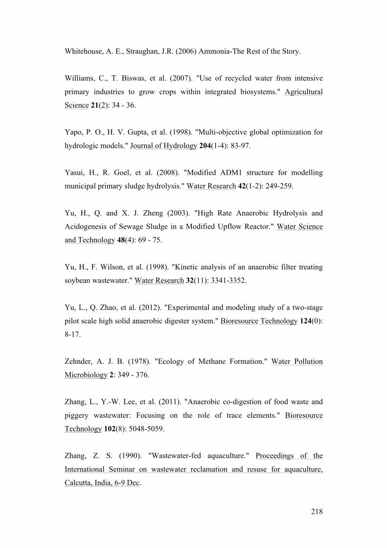
218

Whitehouse, A. E., Straughan, J.R. (2006) Ammonia-The Rest of the Story.

Williams, C., T. Biswas, et al. (2007). "Use of recycled water from intensive

primary industries to grow crops within integrated biosystems." Agricultural

Science 21(2): 34 - 36.

Yapo, P. O., H. V. Gupta, et al. (1998). "Multi-objective global optimization for

hydrologic models." Journal of Hydrology 204(1-4): 83-97.

Yasui, H., R. Goel, et al. (2008). "Modified ADM1 structure for modelling

municipal primary sludge hydrolysis." Water Research 42(1-2): 249-259.

Yu, H., Q. and X. J. Zheng (2003). "High Rate Anaerobic Hydrolysis and

Acidogenesis of Sewage Sludge in a Modified Upflow Reactor." Water Science

and Technology 48(4): 69 - 75.

Yu, H., F. Wilson, et al. (1998). "Kinetic analysis of an anaerobic filter treating

soybean wastewater." Water Research 32(11): 3341-3352.

Yu, L., Q. Zhao, et al. (2012). "Experimental and modeling study of a two-stage

pilot scale high solid anaerobic digester system." Bioresource Technology 124(0):

8-17.

Zehnder, A. J. B. (1978). "Ecology of Methane Formation." Water Pollution

Microbiology 2: 349 - 376.

Zhang, L., Y.-W. Lee, et al. (2011). "Anaerobic co-digestion of food waste and

piggery wastewater: Focusing on the role of trace elements." Bioresource

Technology 102(8): 5048-5059.

Zhang, Z. S. (1990). "Wastewater-fed aquaculture." Proceedings of the

International Seminar on wastewater reclamation and resuse for aquaculture,

Calcutta, India, 6-9 Dec.

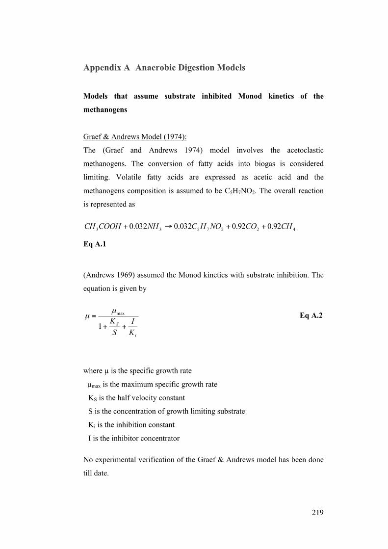
219

Appendix A Anaerobic Digestion Models

Models that assume substrate inhibited Monod kinetics of the

methanogens

Graef & Andrews Model (1974):

The (Graef and Andrews 1974) model involves the acetoclastic

methanogens. The conversion of fatty acids into biogas is considered

limiting. Volatile fatty acids are expressed as acetic acid and the

methanogens composition is assumed to be C5H7NO2. The overall reaction

is represented as

4227533 92.092.0032.0032.0 CHCONOHCNHCOOHCH ++→+

Eq A.1

(Andrews 1969) assumed the Monod kinetics with substrate inhibition. The

equation is given by

i

S

KI

SK

++=1

maxµµ Eq A.2

where µ is the specific growth rate

µmax is the maximum specific growth rate

KS is the half velocity constant

S is the concentration of growth limiting substrate

Ki is the inhibition constant

I is the inhibitor concentrator

No experimental verification of the Graef & Andrews model has been done

till date.

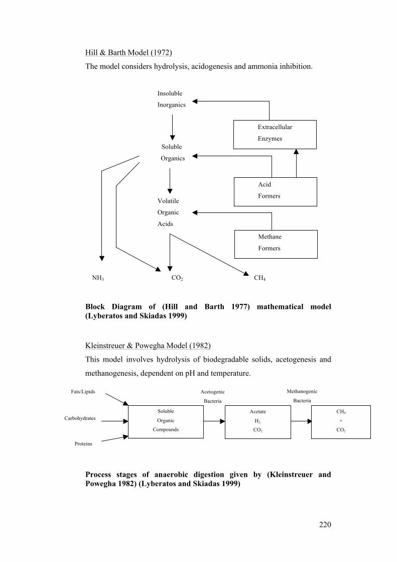
220

Hill & Barth Model (1972)

The model considers hydrolysis, acidogenesis and ammonia inhibition.

Block Diagram of (Hill and Barth 1977) mathematical model (Lyberatos and Skiadas 1999)

Kleinstreuer & Powegha Model (1982)

This model involves hydrolysis of biodegradable solids, acetogenesis and

methanogenesis, dependent on pH and temperature.

Process stages of anaerobic digestion given by (Kleinstreuer and Powegha 1982) (Lyberatos and Skiadas 1999)

Insoluble

Inorganics

Soluble

Organics

Volatile

Organic

Acids

CO2

Extracellular

Enzymes

Acid

Formers

Methane

Formers

CH4 NH3

Fats/Lipids

Carbohydrates

Proteins

Acetogenic

Bacteria

Methanogenic

Bacteria

Soluble

Organic

Compounds

Acetate

H2,

CO2

CH4

+

CO2

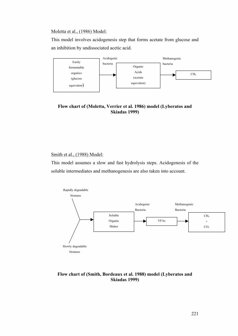
221

Moletta et al., (1986) Model:

This model involves acidogenesis step that forms acetate from glucose and

an inhibition by undissociated acetic acid.

Flow chart of (Moletta, Verrier et al. 1986) model (Lyberatos and Skiadas 1999)

Smith et al., (1988) Model:

This model assumes a slow and fast hydrolysis steps. Acidogenesis of the

soluble intermediates and methanogenesis are also taken into account.

Flow chart of (Smith, Bordeaux et al. 1988) model (Lyberatos and Skiadas 1999)

Acidogenic

bacteria Methanogenic

bacteria Easily

fermentable

organics

(glucose

equivalent)

Organic

Acids

(acetate

equivalent)

CH4

VFAs

Rapidly degradable

biomass

Slowly degradable

biomass

Acidogenic

Bacteria

Methanogenic

Bacteria

Soluble

Organic

Matter

CH4

+

CO2

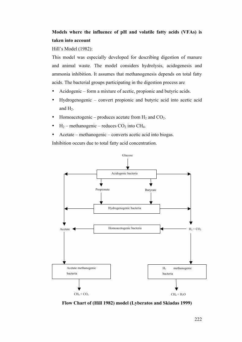
222

Models where the influence of pH and volatile fatty acids (VFAs) is

taken into account

Hill’s Model (1982):

This model was especially developed for describing digestion of manure

and animal waste. The model considers hydrolysis, acidogenesis and

ammonia inhibition. It assumes that methanogenesis depends on total fatty

acids. The bacterial groups participating in the digestion process are

• Acidogenic – form a mixture of acetic, propionic and butyric acids.

• Hydrogenogenic – convert propionic and butyric acid into acetic acid

and H2.

• Homoacetogenic – produces acetate from H2 and CO2.

• H2 – methanogenic – reduces CO2 into CH4.

• Acetate – methanogenic – converts acetic acid into biogas.

Inhibition occurs due to total fatty acid concentration.

Flow Chart of (Hill 1982) model (Lyberatos and Skiadas 1999)

Glucose

Acidogenic bacteria

Hydrogenogenic bacteria

Homoacetogenic bacteria

Acetate methanogenic

bacteria H2 methanogenic

bacteria

CH4 + CO2 CH4 + H2O

H2 + CO2 Acetate

Propionate Butyrate

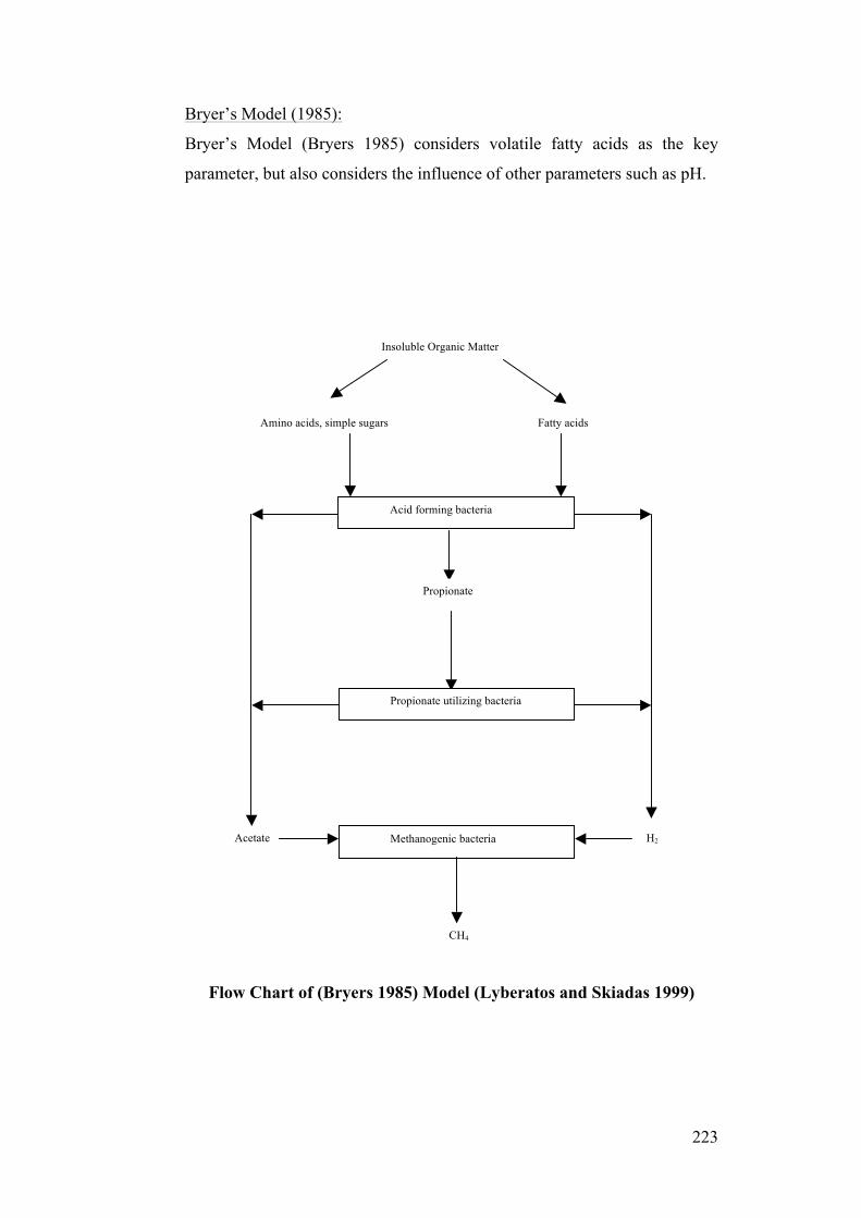
223

Bryer’s Model (1985):

Bryer’s Model (Bryers 1985) considers volatile fatty acids as the key

parameter, but also considers the influence of other parameters such as pH.

Flow Chart of (Bryers 1985) Model (Lyberatos and Skiadas 1999)

Insoluble Organic Matter

Amino acids, simple sugars Fatty acids

Acid forming bacteria

Propionate

Propionate utilizing bacteria

Methanogenic bacteria Acetate H2

CH4

224

Models where the process is primarily controlled by the H2

concentration in the reactor

Mosey’s Model (1983):

(Mosey 1983) considered the H2 partial pressure as the key regulatory

parameter of the anaerobic digestion of glucose. The model considers four

bacterial groups to participate in the conversion of glucose to CO2 and CH4.

• The acid forming bacteria which ferment glucose to produce a mixture

of acetate, propionate and butyrate.

• The acetogenic bacteria convert the propionate and butyrate to acetate.

• The acetoclastic methane bacteria convert acetate to CO2 and CH4.

• The hydrogen utilizing methane bacteria reduce CO2 to CH4.

Mosey found that the hydrogen partial pressure also influences the

acetogenic growth rate, since high values inhibit the generation of propionic

and butyric acids. According to the Mosey model, a sudden increase in the

organic loading rate is expected to cause an accumulation of VFAs since

acetogens grow at a slower rate than the acidogens.

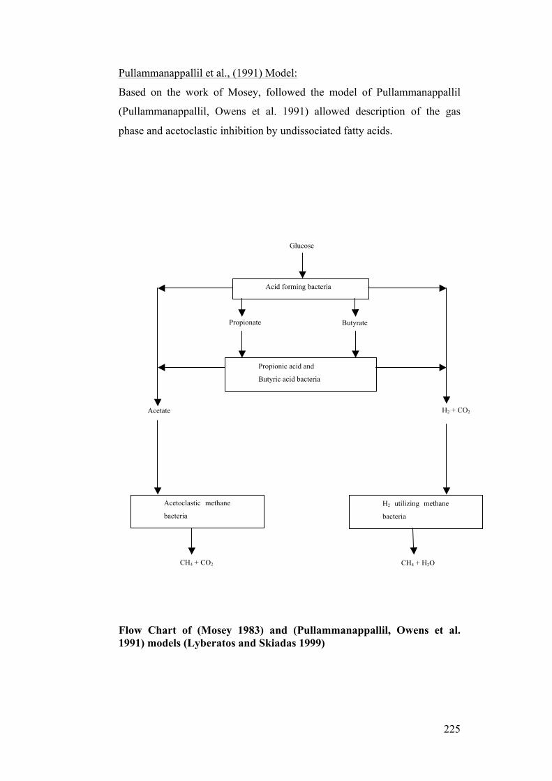
225

Pullammanappallil et al., (1991) Model:

Based on the work of Mosey, followed the model of Pullammanappallil

(Pullammanappallil, Owens et al. 1991) allowed description of the gas

phase and acetoclastic inhibition by undissociated fatty acids.

Flow Chart of (Mosey 1983) and (Pullammanappallil, Owens et al. 1991) models (Lyberatos and Skiadas 1999)

H2 + CO2 Acetate

Propionate Butyrate

Glucose


Propionic acid and

Butyric acid bacteria

Acetoclastic methane

bacteria

H2 utilizing methane

bacteria

CH4 + CO2 CH4 + H2O

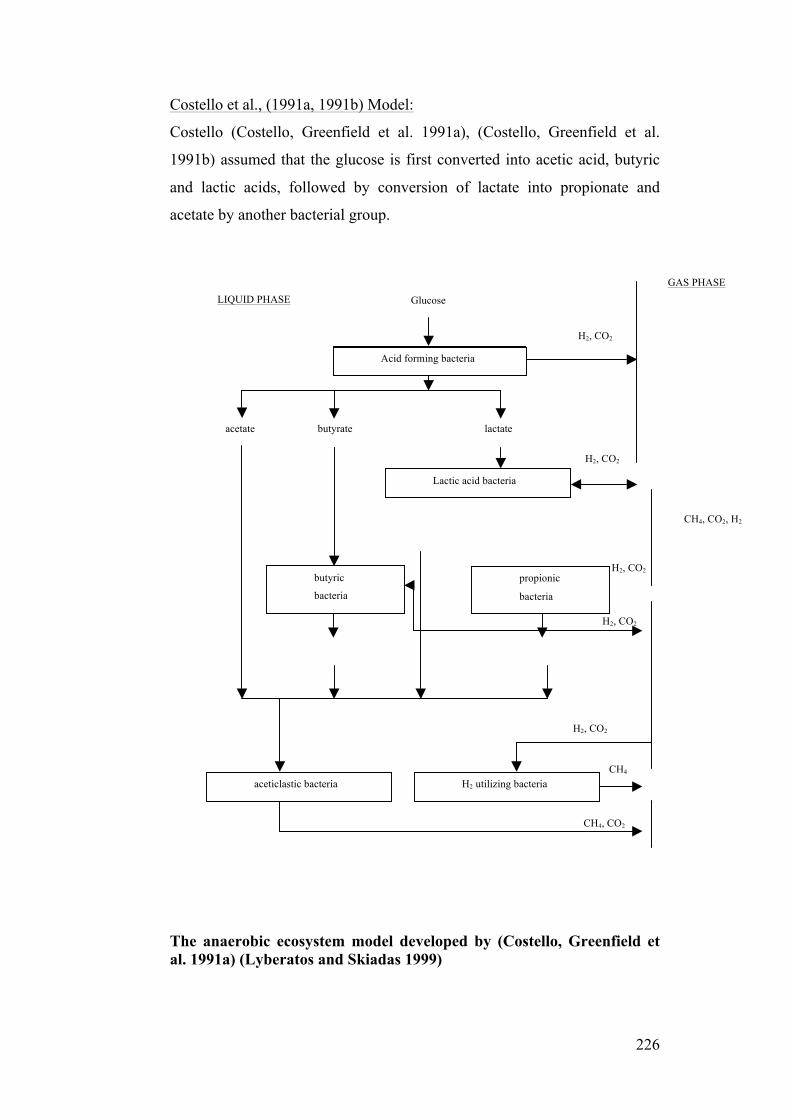
226

Costello et al., (1991a, 1991b) Model:

Costello (Costello, Greenfield et al. 1991a), (Costello, Greenfield et al.

1991b) assumed that the glucose is first converted into acetic acid, butyric

and lactic acids, followed by conversion of lactate into propionate and

acetate by another bacterial group.

The anaerobic ecosystem model developed by (Costello, Greenfield et al. 1991a) (Lyberatos and Skiadas 1999)

CH4

CH4, CO2

H2, CO2

H2, CO2

H2, CO2

CH4, CO2, H2

Glucose


acetate butyrate lactate

H2, CO2

H2, CO2

LIQUID PHASE GAS PHASE

Glucose LIQUID PHASE

butyric

bacteria

propionic

bacteria

aceticlastic bacteria H2 utilizing bacteria


Lactic acid bacteria

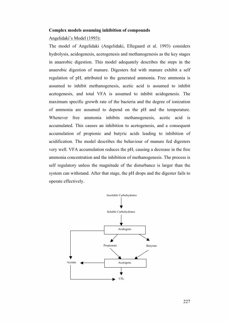
227

Complex models assuming inhibition of compounds

Angelidaki’s Model (1993):

The model of Angelidaki (Angelidaki, Ellegaard et al. 1993) considers

hydrolysis, acidogenesis, acetogenesis and methanogenesis as the key stages

in anaerobic digestion. This model adequately describes the steps in the

anaerobic digestion of manure. Digesters fed with manure exhibit a self

regulation of pH, attributed to the generated ammonia. Free ammonia is

assumed to inhibit methanogenesis, acetic acid is assumed to inhibit

acetogenesis, and total VFA is assumed to inhibit acidogenesis. The

maximum specific growth rate of the bacteria and the degree of ionization

of ammonia are assumed to depend on the pH and the temperature.

Whenever free ammonia inhibits methanogenesis, acetic acid is

accumulated. This causes an inhibition to acetogenesis, and a consequent

accumulation of propionic and butyric acids leading to inhibition of

acidification. The model describes the behaviour of manure fed digesters

very well. VFA accumulation reduces the pH, causing a decrease in the free

ammonia concentration and the inhibition of methanogenesis. The process is

self regulatory unless the magnitude of the disturbance is larger than the

system can withstand. After that stage, the pH drops and the digester fails to

operate effectively.

Insoluble Carbohydrates

Soluble Carbohydrates

Acidogens

Acetogens

Propionate Butyrate

CH4

Acetate

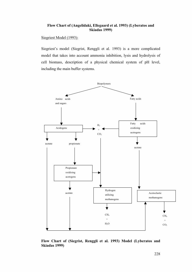
228

Flow Chart of (Angelidaki, Ellegaard et al. 1993) (Lyberatos and Skiadas 1999)

Siegriest Model (1993):

Siegriest’s model (Siegrist, Renggli et al. 1993) is a more complicated

model that takes into account ammonia inhibition, lysis and hydrolysis of

cell biomass, description of a physical chemical system of pH level,

including the main buffer systems.

Flow Chart of (Siegrist, Renggli et al. 1993) Model (Lyberatos and Skiadas 1999)

acetate

CH4

+

H2O

CH4

+

CO2

Propionate

oxidizing

acetogens

Hydrogen

utilizing

methanogens

Acetoclastic

methanogens

acetate propionate acetate

Fatty acids

oxidizing

acetogens

Acidogens H2

+

CO2

Fatty acids

Biopolymers

Amino acids

and sugars

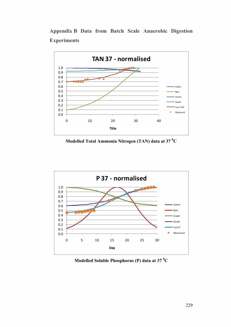
229

Appendix B Data from Batch Scale Anaerobic Digestion

Experiments

Modelled Total Ammonia Nitrogen (TAN) data at 37 0C

Modelled Soluble Phosphorus (P) data at 37 0C

0.00.10.20.30.40.50.60.70.80.91.0

0 10 20 30 40

Title


Substr

Bact

Grwth

Death

Cum TAN

Measured

0.00.10.20.30.40.50.60.70.80.91.0

0 5 10 15 20 25 30

Day


Substr

Bact

Grwth

Death

Cum P

Measured

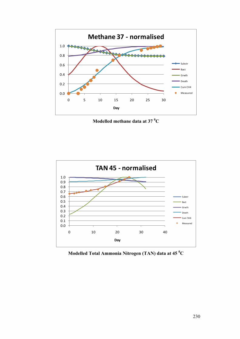
230

Modelled methane data at 37 0C

Modelled Total Ammonia Nitrogen (TAN) data at 45 0C

0.0

0.2

0.4

0.6

0.8

1.0

0 5 10 15 20 25 30

Day


Substr

Bact

Grwth

Death

Cum CH4

Measured

0.00.10.20.30.40.50.60.70.80.91.0

0 10 20 30 40

Day


Substr

Bact

Grwth

Death

Cum TAN

Measured

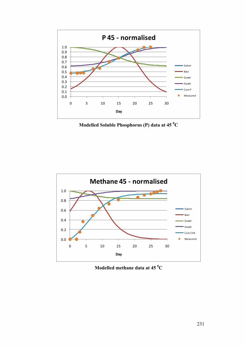
231

Modelled Soluble Phosphorus (P) data at 45 0C

Modelled methane data at 45 0C

0.00.10.20.30.40.50.60.70.80.91.0

0 5 10 15 20 25 30

Day


Substr

Bact

Grwth

Death

Cum P

Measured

0.0

0.2

0.4

0.6

0.8

1.0

0 5 10 15 20 25 30

Day


Substr

Bact

Grwth

Death

Cum CH4

Measured

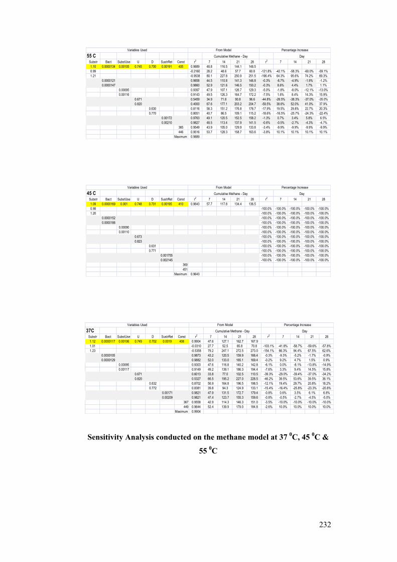
232

Sensitivity Analysis conducted on the methane model at 37 0C, 45 0C &

55 0C

55 CSubstr Bact SubstUse U D SustrRet Const r2 7 14 21 28 r2 7 14 21 281.10 0.0000134 0.00105 0.745 0.700 0.00191 405 0.9889 48.8 116.5 144.1 148.50.99 -0.2160 28.2 48.6 57.7 60.8 -121.8% -42.1% -58.3% -60.0% -59.1%1.21 -0.9538 80.1 227.8 250.9 251.5 -196.4% 64.3% 95.6% 74.2% 69.3%

0.0000121 0.9858 44.5 110.8 141.3 146.8 -0.3% -8.7% -4.9% -1.9% -1.2%0.0000147 0.9860 52.9 121.6 146.5 150.2 -0.3% 8.6% 4.4% 1.7% 1.1%

0.00095 0.9397 47.9 107.1 126.7 129.3 -5.0% -1.8% -8.0% -12.1% -13.0%0.00116 0.9143 49.5 126.3 164.7 172.2 -7.5% 1.6% 8.4% 14.3% 15.9%

0.671 0.5459 34.9 71.8 90.8 96.6 -44.8% -28.5% -38.3% -37.0% -35.0%0.820 0.4000 67.6 177.1 203.2 204.7 -59.5% 38.6% 52.0% 41.0% 37.9%

0.630 0.8116 58.3 151.2 176.8 178.7 -17.9% 19.5% 29.8% 22.7% 20.3%0.770 0.8051 40.7 86.5 109.1 115.2 -18.6% -16.5% -25.7% -24.3% -22.4%

0.00172 0.9763 49.1 120.5 152.5 158.2 -1.3% 0.7% 3.4% 5.8% 6.5%0.00210 0.9827 48.5 113.4 137.9 141.5 -0.6% -0.5% -2.7% -4.3% -4.7%

365 0.9549 43.9 105.0 129.9 133.8 -3.4% -9.9% -9.9% -9.9% -9.9%446 0.9516 53.7 128.3 158.7 163.6 -3.8% 10.1% 10.1% 10.1% 10.1%

Maximum 0.9889

Variables Used From Model Percentage Increase

Cumulative Methane - Day Day

45 CSubstr Bact SubstUse U D SustrRet Const r2 7 14 21 28 r2 7 14 21 281.09 0.0000169 0.001 0.748 0.701 0.00195 410 0.9643 57.7 117.8 134.4 136.50.98 -100.0% -100.0% -100.0% -100.0% -100.0%1.20 -100.0% -100.0% -100.0% -100.0% -100.0%

0.0000152 -100.0% -100.0% -100.0% -100.0% -100.0%0.0000186 -100.0% -100.0% -100.0% -100.0% -100.0%

0.00090 -100.0% -100.0% -100.0% -100.0% -100.0%0.00110 -100.0% -100.0% -100.0% -100.0% -100.0%

0.673 -100.0% -100.0% -100.0% -100.0% -100.0%0.823 -100.0% -100.0% -100.0% -100.0% -100.0%

0.631 -100.0% -100.0% -100.0% -100.0% -100.0%0.771 -100.0% -100.0% -100.0% -100.0% -100.0%

0.001755 -100.0% -100.0% -100.0% -100.0% -100.0%0.002145 -100.0% -100.0% -100.0% -100.0% -100.0%

369451

Maximum 0.9643



37CSubstr Bact SubstUse U D SustrRet Const r2 7 14 21 28 r2 7 14 21 281.12 0.0000117 0.00106 0.745 0.702 0.0019 408 0.9904 47.6 127.1 162.7 167.91.01 -0.0310 27.7 52.5 65.8 70.8 -103.1% -41.8% -58.7% -59.6% -57.8%1.23 -0.5358 79.2 247.1 272.5 273.0 -154.1% 66.3% 94.4% 67.5% 62.6%

0.0000105 0.9873 43.2 120.5 159.9 166.4 -0.3% -9.3% -5.2% -1.7% -0.9%0.0000129 0.9882 52.0 133.0 165.1 169.4 -0.2% 9.2% 4.7% 1.5% 0.9%

0.00095 0.9303 47.6 116.8 140.2 142.8 -6.1% 0.0% -8.1% -13.8% -14.9%0.00117 0.9149 49.2 139.1 186.3 194.4 -7.6% 3.3% 9.4% 14.5% 15.8%

0.671 0.6013 33.8 77.0 102.5 110.5 -39.3% -29.0% -39.4% -37.0% -34.2%0.820 0.5327 66.5 195.2 227.0 228.5 -46.2% 39.5% 53.6% 39.5% 36.1%

0.632 0.8702 56.9 164.8 196.5 198.5 -12.1% 19.4% 29.7% 20.8% 18.2%0.772 0.8381 39.8 94.3 124.9 133.1 -15.4% -16.4% -25.8% -23.3% -20.8%

0.00171 0.9821 47.9 131.5 172.7 179.4 -0.8% 0.6% 3.5% 6.1% 6.8%0.00209 0.9821 47.4 123.7 155.3 159.6 -0.8% -0.5% -2.7% -4.5% -5.0%

367 0.9558 42.9 114.3 146.3 151.0 -3.5% -10.0% -10.0% -10.0% -10.0%449 0.9644 52.4 139.9 179.0 184.8 -2.6% 10.0% 10.0% 10.0% 10.0%

Maximum 0.9904



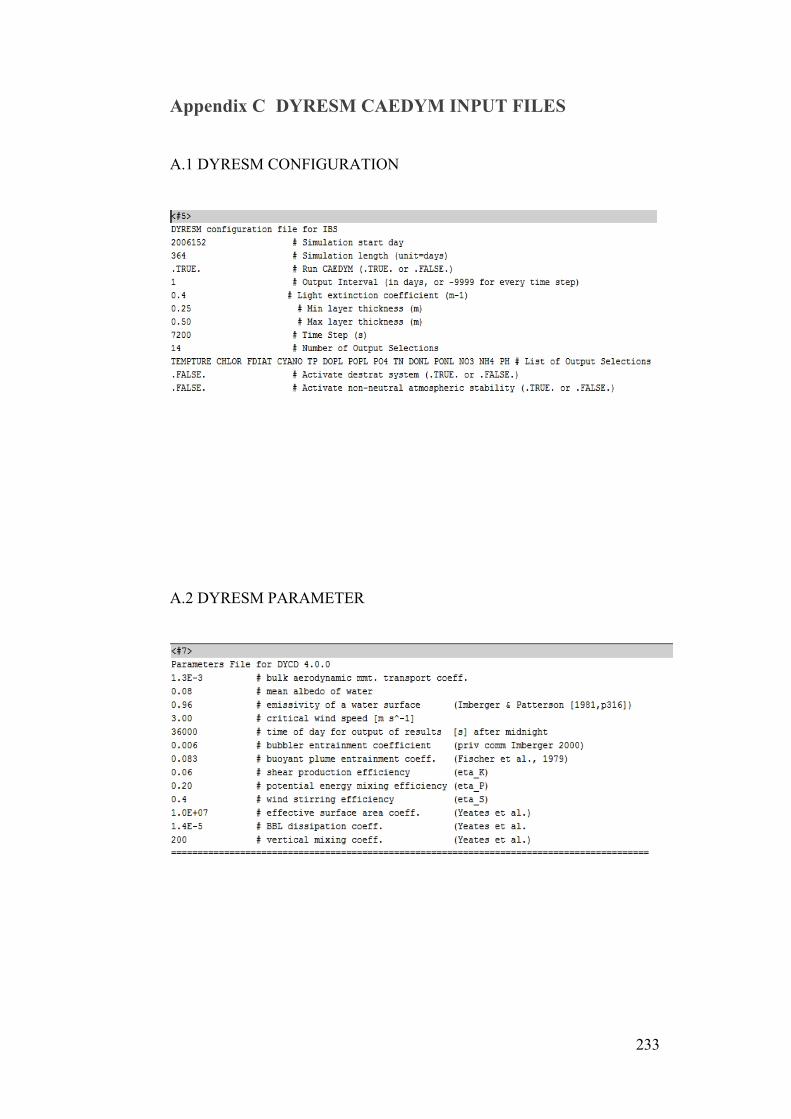
233

Appendix C DYRESM CAEDYM INPUT FILES

A.1 DYRESM CONFIGURATION

A.2 DYRESM PARAMETER

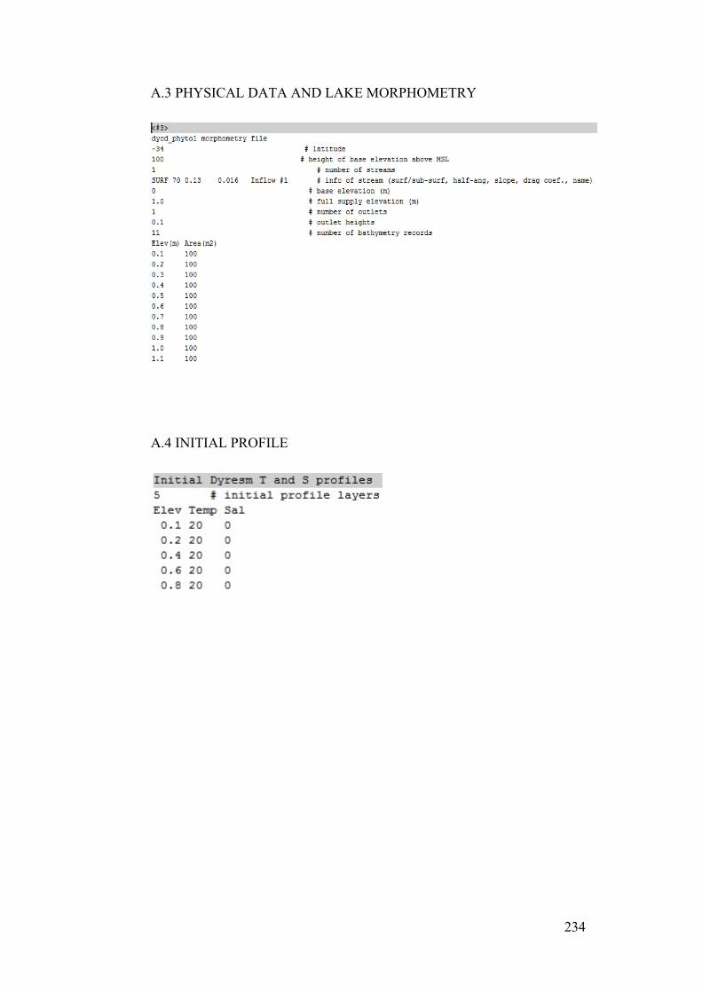
234

A.3 PHYSICAL DATA AND LAKE MORPHOMETRY

A.4 INITIAL PROFILE

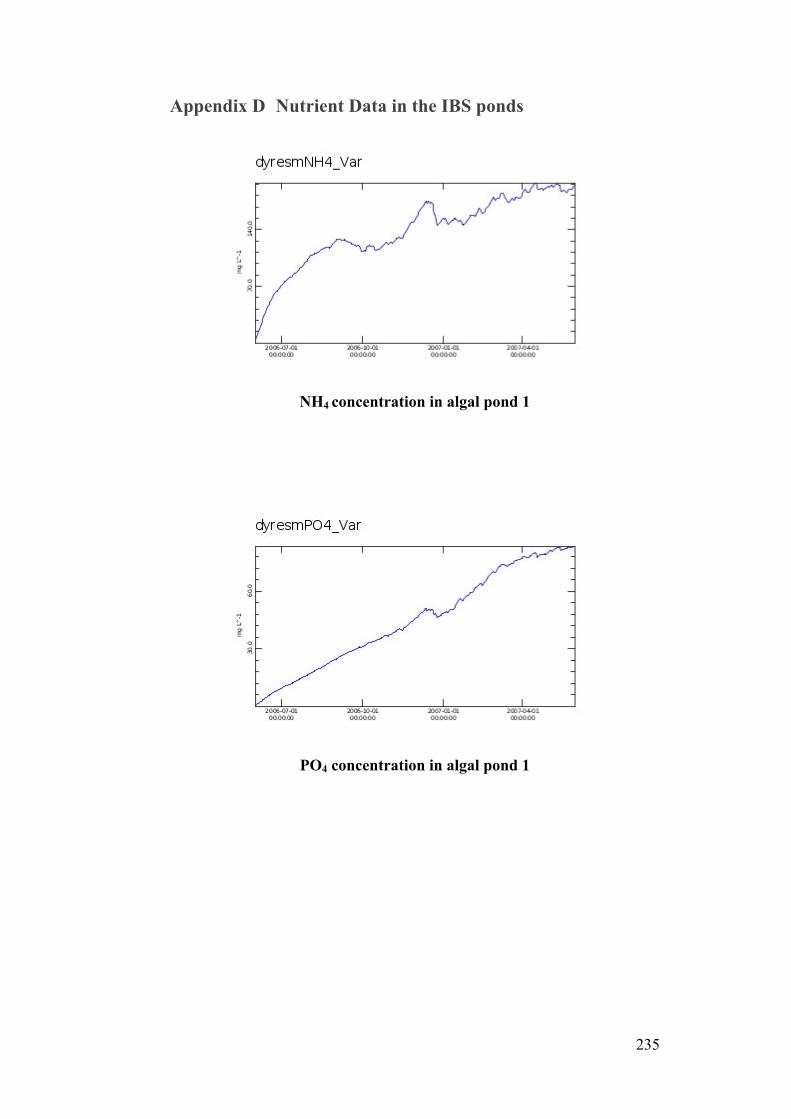
235

Appendix D Nutrient Data in the IBS ponds

NH4 concentration in algal pond 1

PO4 concentration in algal pond 1

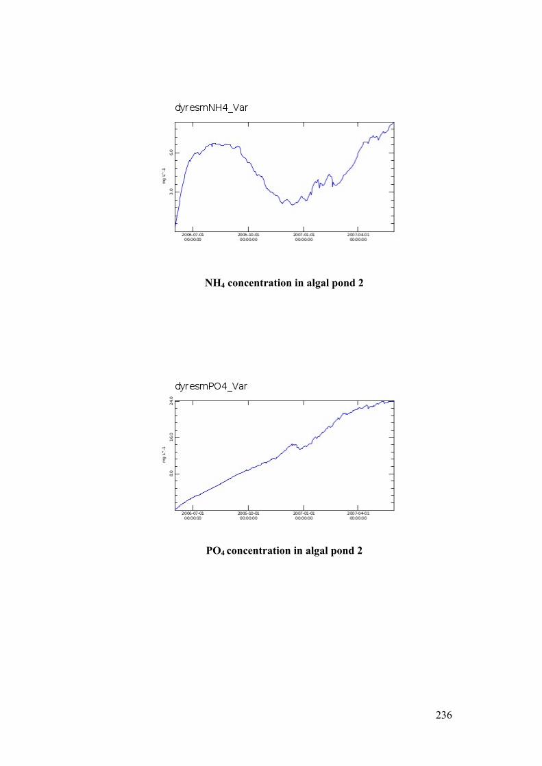
236

NH4 concentration in algal pond 2

PO4 concentration in algal pond 2

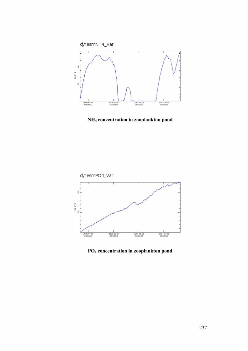
237

NH4 concentration in zooplankton pond

PO4 concentration in zooplankton pond

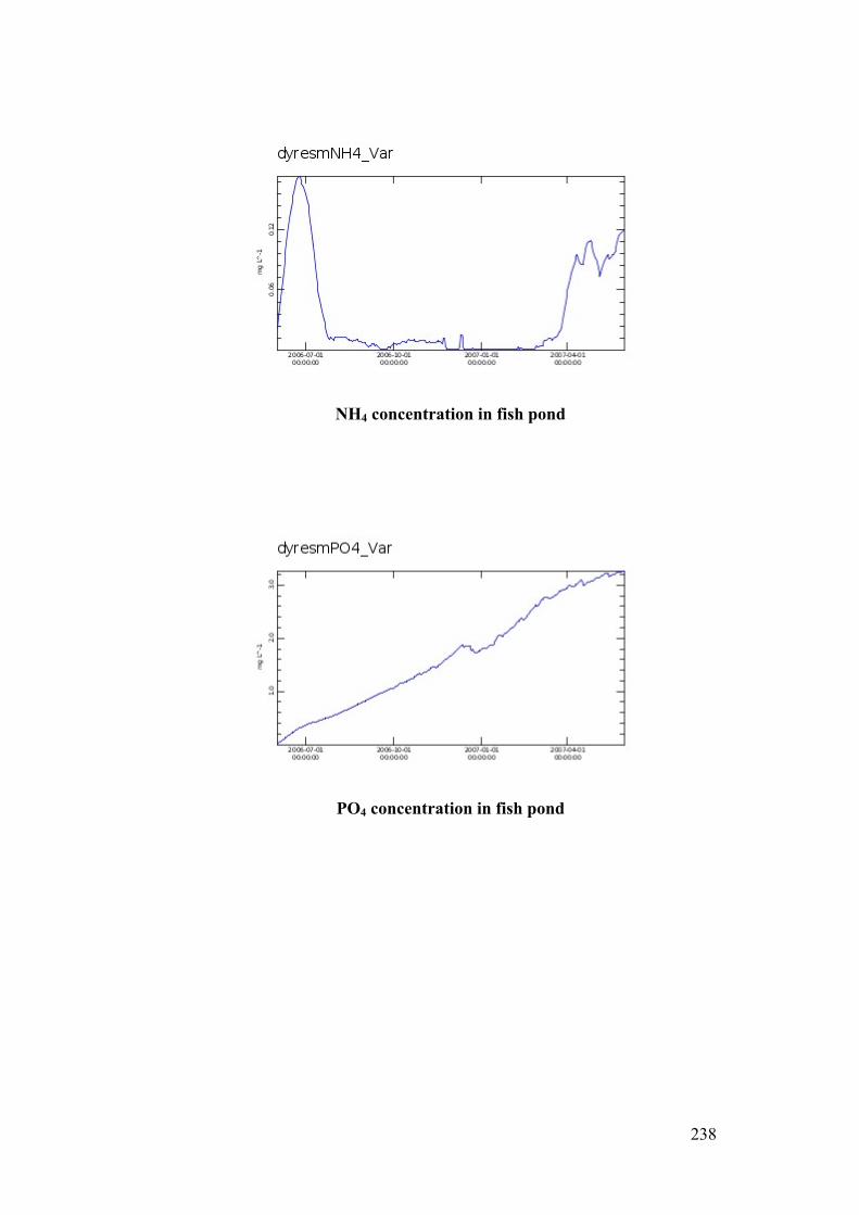
238

NH4 concentration in fish pond

PO4 concentration in fish pond

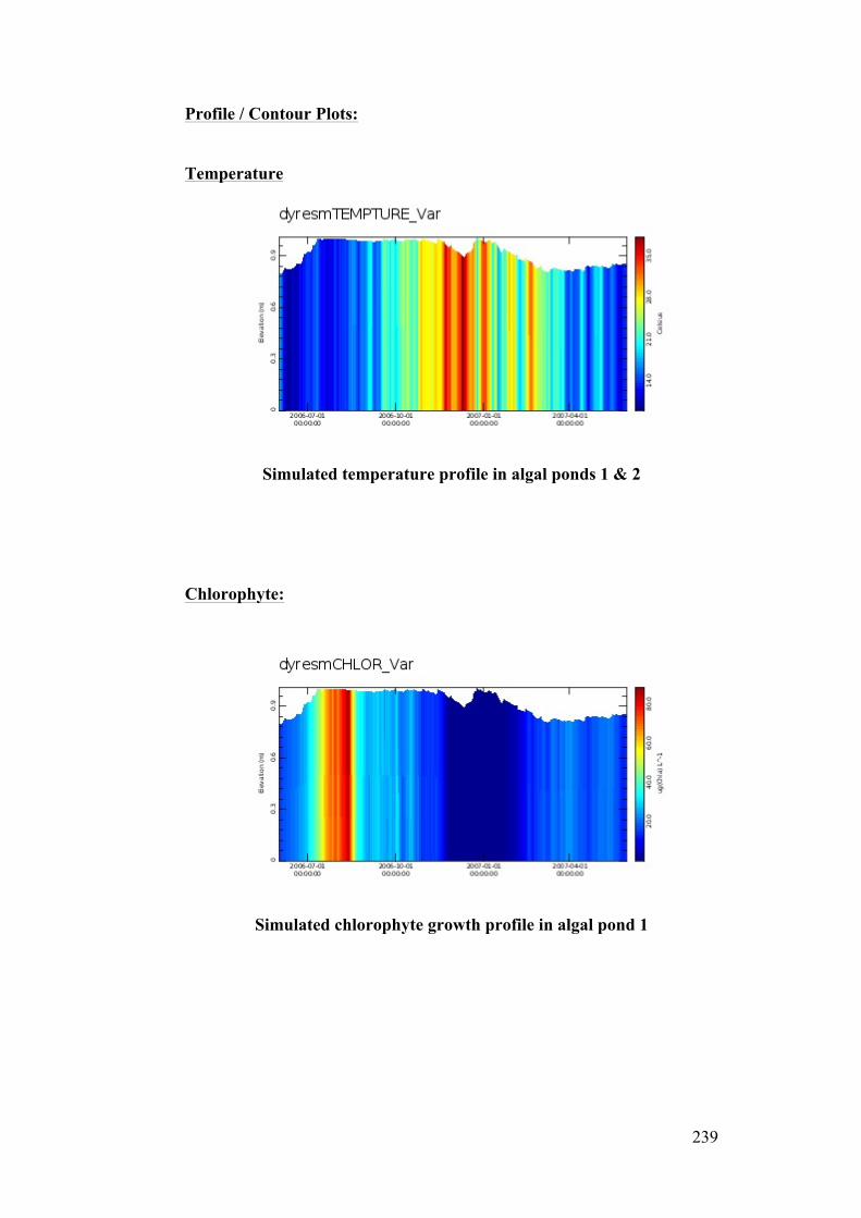
239

Profile / Contour Plots:

Temperature

Simulated temperature profile in algal ponds 1 & 2

Chlorophyte:

Simulated chlorophyte growth profile in algal pond 1

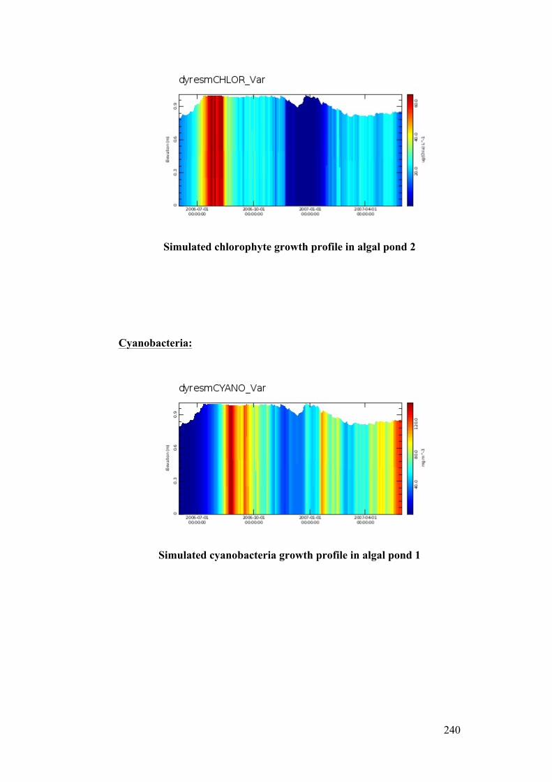
240

Simulated chlorophyte growth profile in algal pond 2

Cyanobacteria:

Simulated cyanobacteria growth profile in algal pond 1

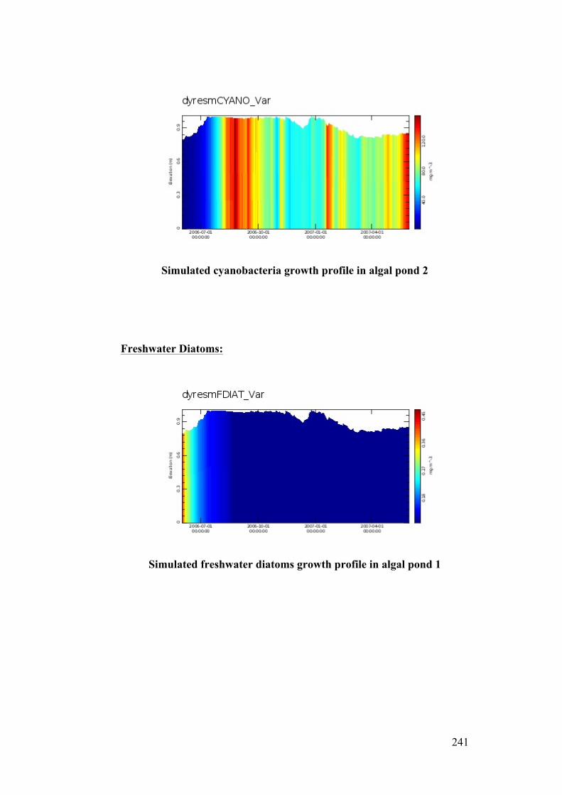
241

Simulated cyanobacteria growth profile in algal pond 2

Freshwater Diatoms:

Simulated freshwater diatoms growth profile in algal pond 1

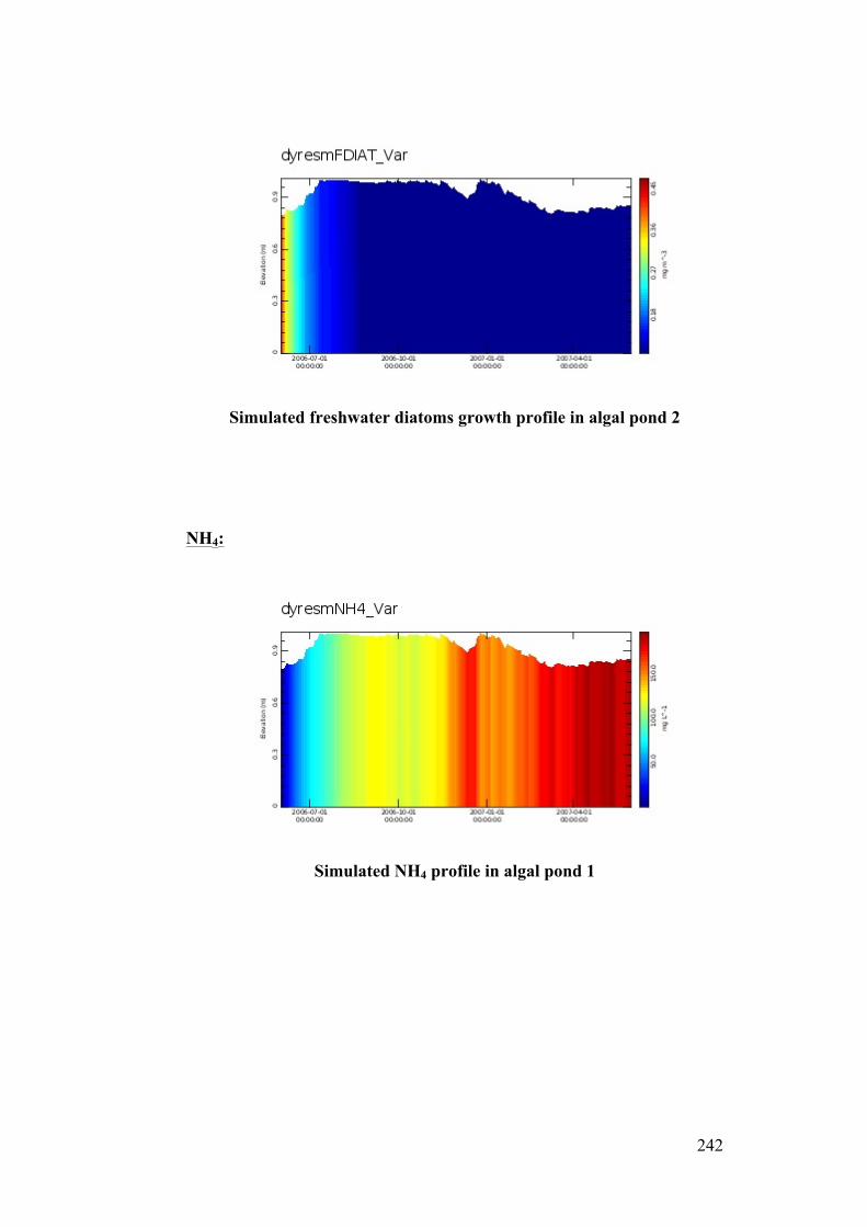
242

Simulated freshwater diatoms growth profile in algal pond 2

NH4:

Simulated NH4 profile in algal pond 1

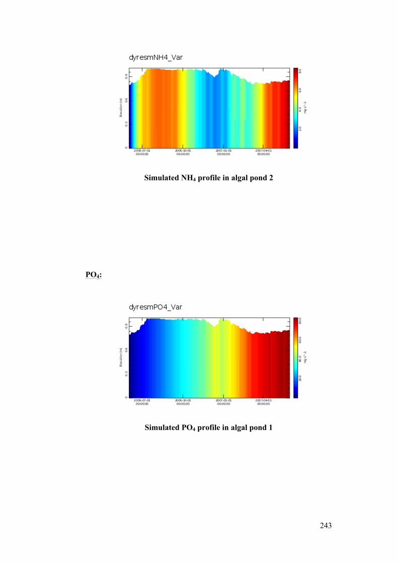
243

Simulated NH4 profile in algal pond 2

PO4:

Simulated PO4 profile in algal pond 1

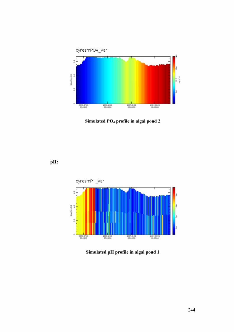
244

Simulated PO4 profile in algal pond 2

pH:

Simulated pH profile in algal pond 1

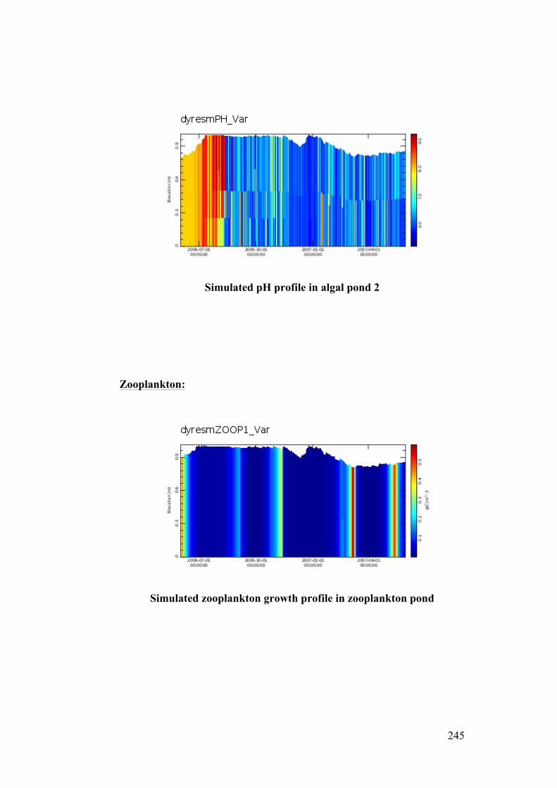
245

Simulated pH profile in algal pond 2

Zooplankton:

Simulated zooplankton growth profile in zooplankton pond

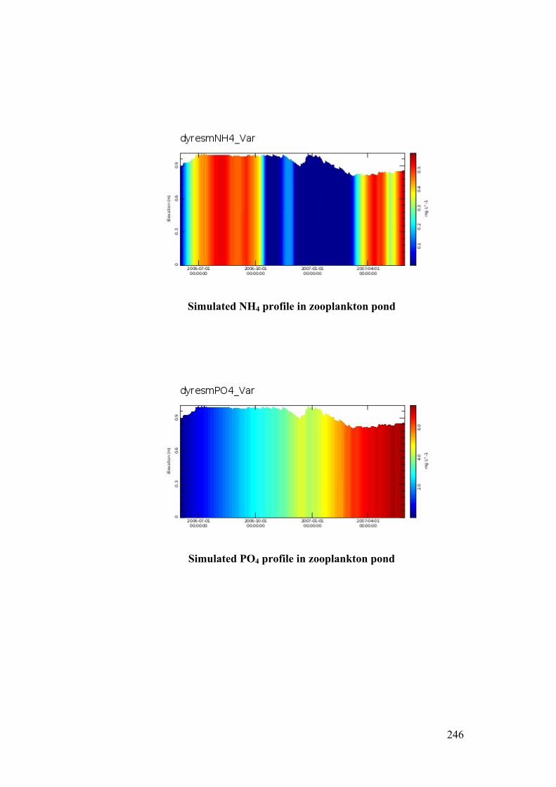
246

Simulated NH4 profile in zooplankton pond

Simulated PO4 profile in zooplankton pond

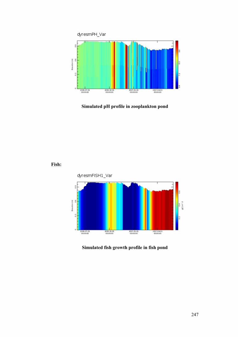
247

Simulated pH profile in zooplankton pond

Fish:

Simulated fish growth profile in fish pond

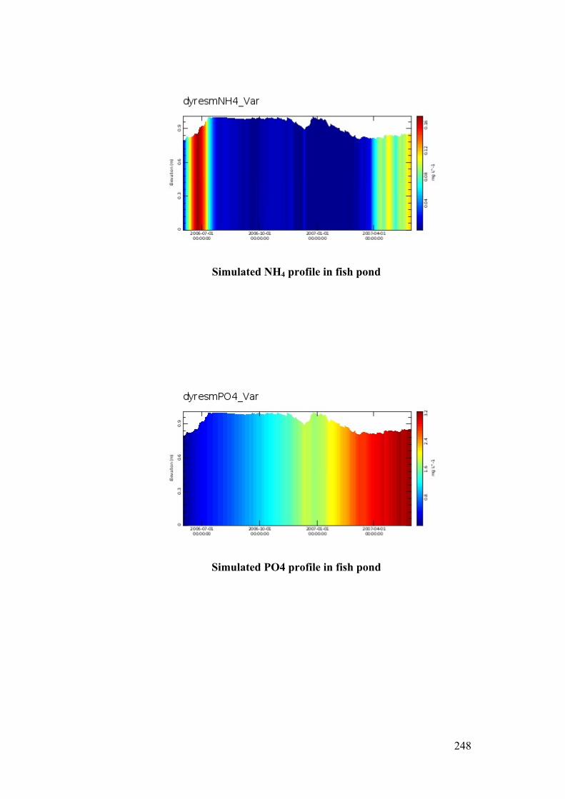
248

Simulated NH4 profile in fish pond

Simulated PO4 profile in fish pond

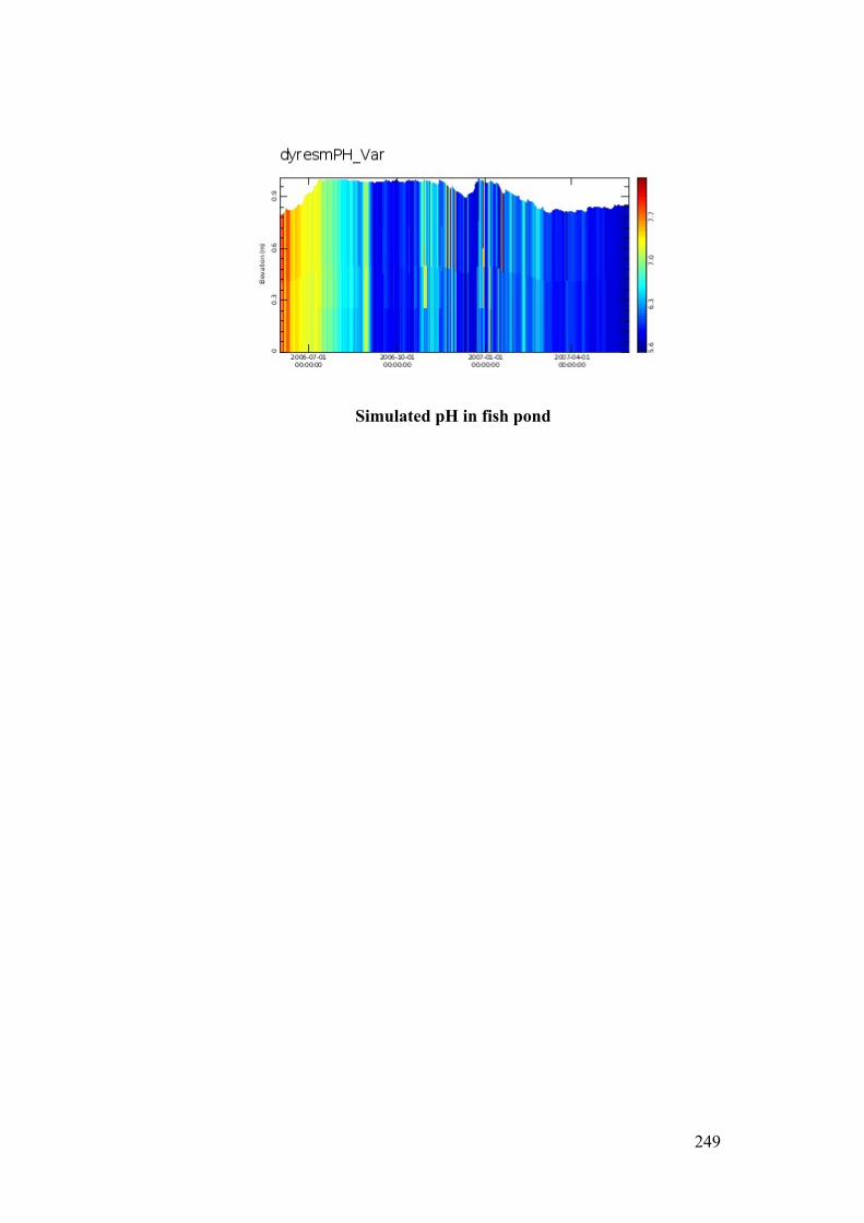
249

Simulated pH in fish pond

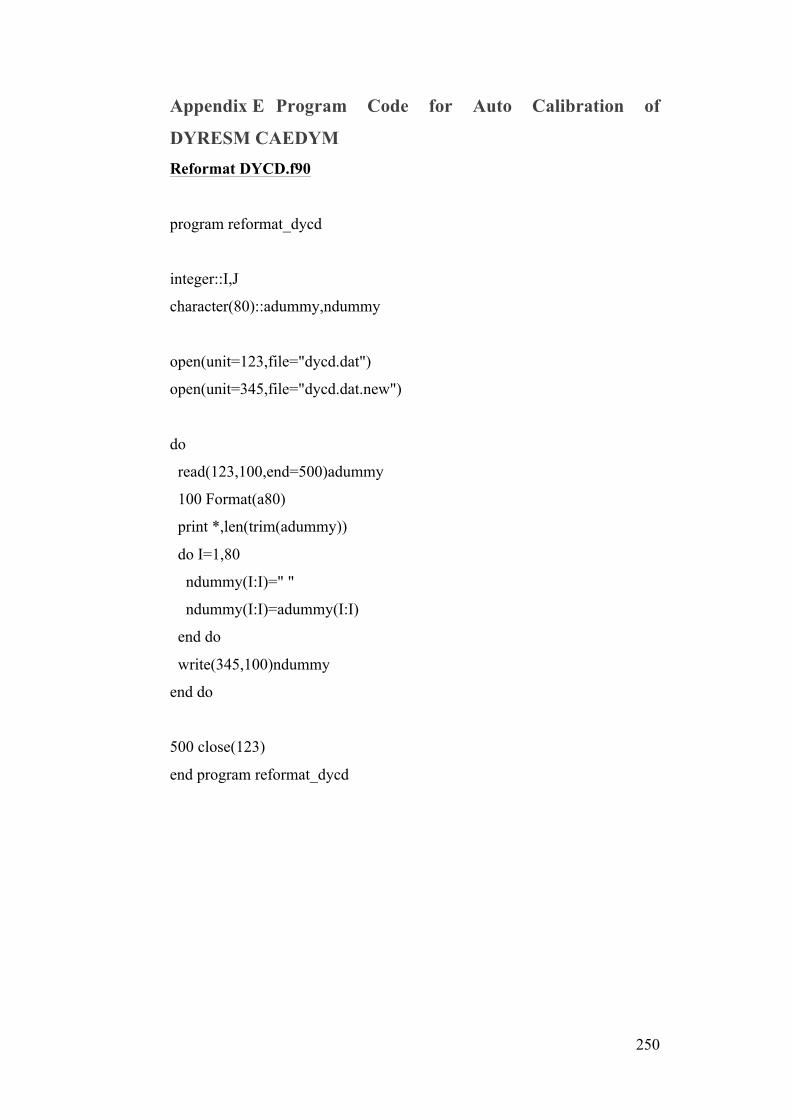
250

Appendix E Program Code for Auto Calibration of

DYRESM CAEDYM Reformat DYCD.f90

program reformat_dycd

integer::I,J

character(80)::adummy,ndummy

open(unit=123,file="dycd.dat")

open(unit=345,file="dycd.dat.new")

do

read(123,100,end=500)adummy

100 Format(a80)

print *,len(trim(adummy))

do I=1,80

ndummy(I:I)=" "

ndummy(I:I)=adummy(I:I)

end do

write(345,100)ndummy

end do

500 close(123)

end program reformat_dycd

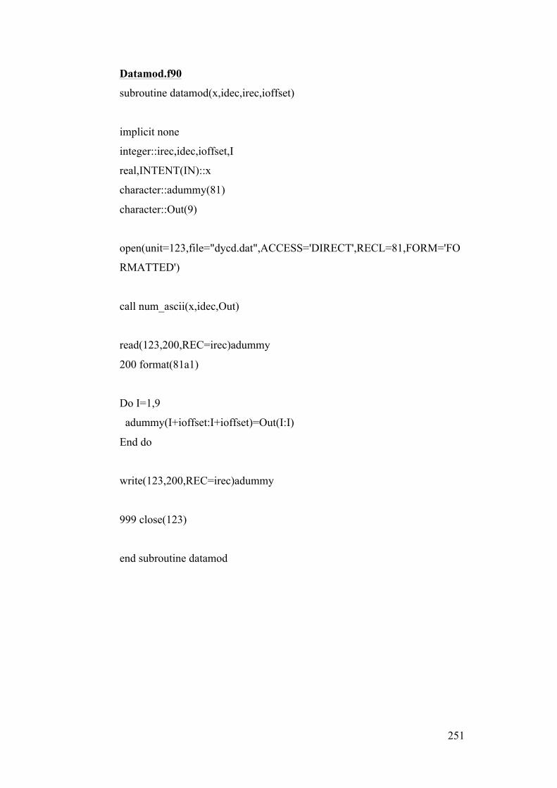
251

Datamod.f90

subroutine datamod(x,idec,irec,ioffset)

implicit none

integer::irec,idec,ioffset,I

real,INTENT(IN)::x

character::adummy(81)

character::Out(9)

open(unit=123,file="dycd.dat",ACCESS='DIRECT',RECL=81,FORM='FO

RMATTED')

call num_ascii(x,idec,Out)

read(123,200,REC=irec)adummy

200 format(81a1)

Do I=1,9

adummy(I+ioffset:I+ioffset)=Out(I:I)

End do

write(123,200,REC=irec)adummy

999 close(123)

end subroutine datamod

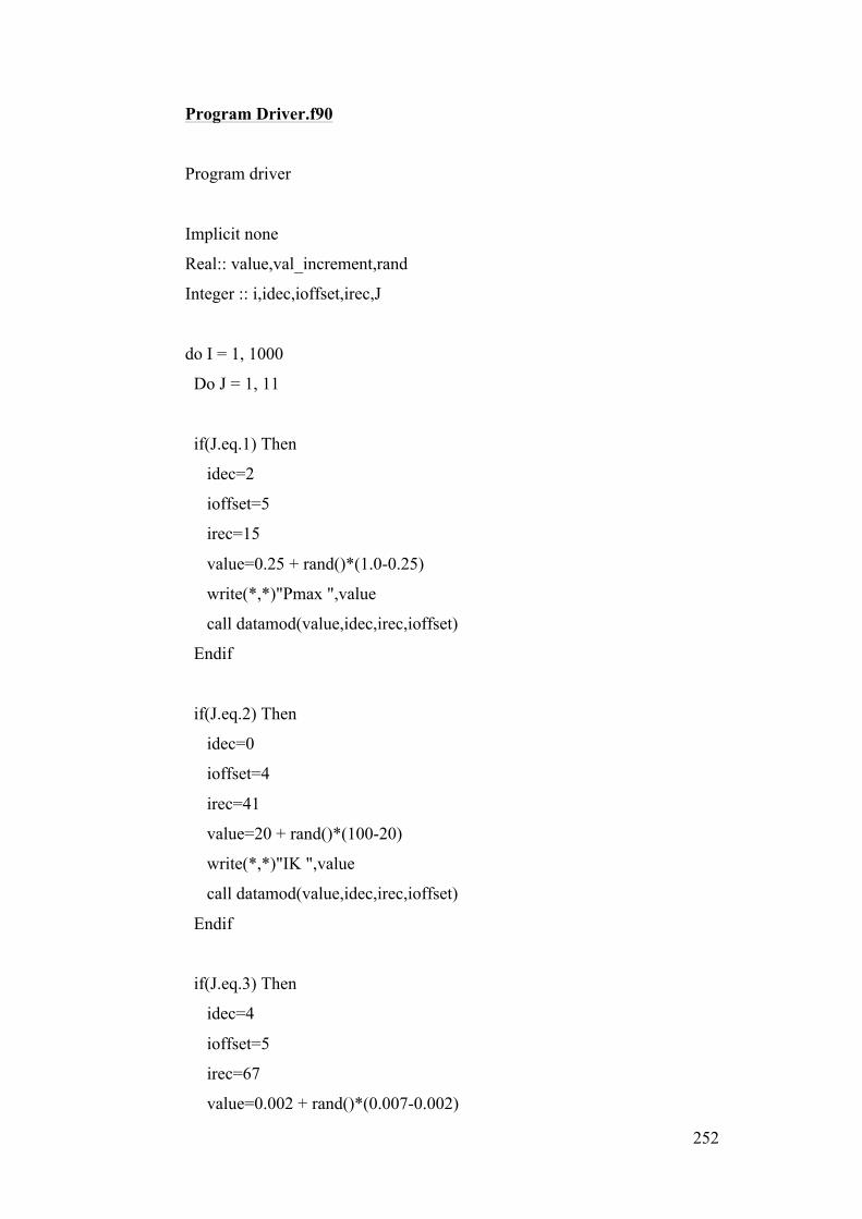
252

Program Driver.f90

Program driver

Implicit none

Real:: value,val_increment,rand

Integer :: i,idec,ioffset,irec,J

do I = 1, 1000

Do J = 1, 11

if(J.eq.1) Then

idec=2

ioffset=5

irec=15

value=0.25 + rand()*(1.0-0.25)

write(*,*)"Pmax ",value

call datamod(value,idec,irec,ioffset)

Endif

if(J.eq.2) Then

idec=0

ioffset=4

irec=41

value=20 + rand()*(100-20)

write(*,*)"IK ",value


Endif

if(J.eq.3) Then

idec=4

ioffset=5

irec=67

value=0.002 + rand()*(0.007-0.002)

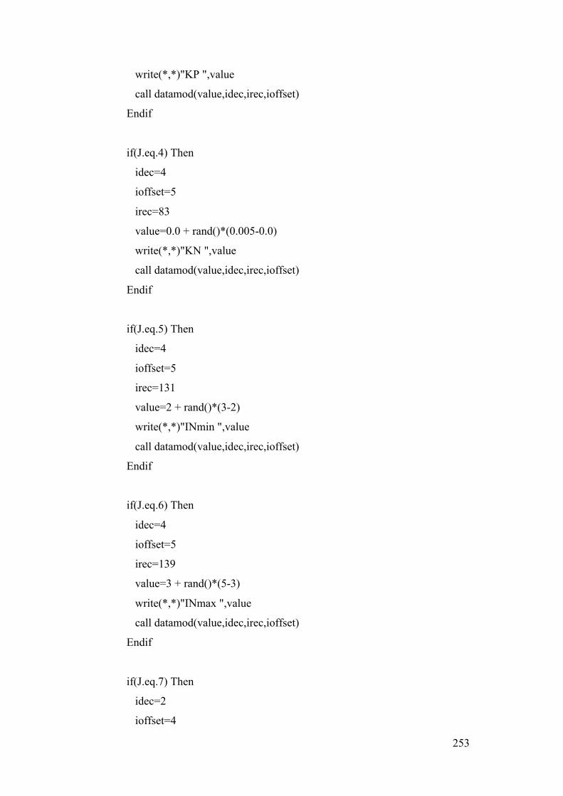
253

write(*,*)"KP ",value


Endif

if(J.eq.4) Then

idec=4

ioffset=5

irec=83

value=0.0 + rand()*(0.005-0.0)

write(*,*)"KN ",value


Endif

if(J.eq.5) Then

idec=4

ioffset=5

irec=131

value=2 + rand()*(3-2)

write(*,*)"INmin ",value


Endif

if(J.eq.6) Then

idec=4

ioffset=5

irec=139

value=3 + rand()*(5-3)

write(*,*)"INmax ",value


Endif

if(J.eq.7) Then

idec=2

ioffset=4

254

irec=147

value=0.25 + rand()*(1-0.25)

write(*,*)"UNmax ",value


Endif

if(J.eq.8) Then

idec=4

ioffset=5

irec=155

value=0.05 + rand()*(0.15-0.05)

write(*,*)"IPmin ",value


Endif

if(J.eq.9) Then

idec=4

ioffset=5

irec=163

value=0.3 + rand()*(0.9-0.3)

write(*,*)"IPmax ",value


Endif

if(J.eq.10) Then

idec=2

ioffset=4

irec=171

value=0.05 + rand()*(0.15-0.05)

write(*,*)"UPmax ",value


Endif

255

if(J.eq.11) Then

idec=4

ioffset=5

irec=271

value=0.06 + rand()*(0.08-0.06)

write(*,*)"kr ",value


Endif

End do

call system("master_run")

call glue_sub()

End do

End

256

Subroutine num_ascii.f90

Subroutine num_ascii(x,idec,Out)

Implicit None

Integer::I,J,K,Irange,Idec,Ipos,Inum,Istart,Ineg

Real,intent(in) ::x

Real ::xx,y

Character::Out(9)

Irange=10000000

xx=x

Do I = 1,9

Out(I:I)=" "

End do

K=1

Inum=9

Istart = 0

Ineg=0

If (xx .lt. 0.0)then

Ineg = 1

xx=Abs(xx)

Endif

Ipos=10**(Idec)

xx=xx*10**Idec

Do I=1,Inum

J = 0

257

y = xx - INT(xx/Irange)*Irange

J = (xx - y)/Irange

If (J .gt. 0 .and. Istart .eq. 0)then

Istart=1

If(Ineg .eq. 1) then

Out(K:K)="-"

K = K + 1

Endif

Endif

If(Istart .eq. 1)then

xx = xx - J*Irange

Out(K:K)=Char(J+48)

K = K + 1

Endif

If(Ipos .eq. Irange)Then

If(Ineg .eq. 1 .and. Istart .eq. 0) then

Out(K:K)="-"

K = K + 1

Endif

Out(K:K)="."

Istart = 1

K = K + 1

Endif

Irange=Irange/10

End do

Return

End

258

Subroutine Glue_sub.f90

Subroutine glue_sub

Implicit none

integer::i,j,p,q,u,v

real(8)::x,y,errcl,sumerrcl=0.0,avgcly,totalcl=0.0,sumvarcl=0.0,NScl

real(8)::dummy1,dummy2,dummy3

real(8):: varcl

totalcl=0

!This part of the program is for chlorophyte calibration

open(unit=123,file="fldcyano.txt")

do i=1,364

read(123,*),y

totalcl=totalcl+y

!print*,y

end do

close(123)

avgcly=totalcl/364

sumerrcl=0

sumvarcl=0

open(unit=222,file="Files/CYANO.ITS")

open(unit=333,file="fldcyano.txt")

do j=1,364

read(222,*),dummy1,x

read(333,*),y

errcl=(x-y)**2

sumerrcl=sumerrcl+errcl

varcl=(y-avgcly)**2

sumvarcl=sumvarcl+varcl

!print*,x,y

259

end do

NScl=1-(sumerrcl/sumvarcl)

write(*,345)NScl

345 format(f10.6," ")

close(222)

close(333)

return

end subroutine glue_sub

260

Appendix F GLUE Calibration Numerical Outputs

Pmax 0.3000495

IK 162.7549

KP 1.6013525E-02

KN 1.8916111E-02

INmin 2.967956

INmax 6.896898

UNmax 1.514976

IPmin 0.3194025

IPmax 2.262906

UPmax 0.4230537

kr 8.1790954E-02

-1.138279

Pmax 1.532858

IK 237.3345

KP 1.8095667E-02

KN 1.5919188E-02

INmin 2.511713

INmax 13.76634

UNmax 1.995085

IPmin 0.4178635

IPmax 2.966611

UPmax 0.2891307

kr 8.8521019E-02

-0.222198

Pmax 2.278895

IK 247.9498

KP 1.9015342E-02

KN 1.9615330E-02

INmin 2.164713

INmax 13.57987

261

UNmax 1.906845

IPmin 0.2882079

IPmax 2.936244

UPmax 0.3243934

kr 8.6169131E-02

-2.921868

Pmax 1.432764

IK 209.3145

KP 1.7897844E-02

KN 1.6891414E-02

INmin 2.544273

INmax 10.92407

UNmax 1.093630

IPmin 0.3828454

IPmax 2.432260

UPmax 0.3798648

kr 9.6898548E-02

0.403511

Pmax 1.383240

IK 265.9270

KP 1.0716619E-02

KN 1.1918589E-02

INmin 2.223608

INmax 12.80367

UNmax 1.083967

IPmin 0.2544030

IPmax 2.616697

UPmax 0.3737425

kr 9.4786234E-02

0.733218

262

Pmax 0.9910892

IK 215.8265

KP 1.4119846E-02

KN 1.9088892E-02

INmin 2.992306

INmax 10.77058

UNmax 1.163922

IPmin 0.4095565

IPmax 2.334848

UPmax 0.3367347

kr 8.1524365E-02

-0.795741

Pmax 0.5833541

IK 176.1786

KP 1.4417774E-02

KN 1.0372999E-02

INmin 2.504163

INmax 9.674148

UNmax 1.579016

IPmin 0.4022338

IPmax 2.093411

UPmax 0.2200110

kr 9.6654058E-02

-1.099454

Pmax 1.157521

IK 178.6295

KP 1.1653987E-02

KN 1.9585462E-02

INmin 2.990804

INmax 6.135645

UNmax 1.870639

IPmin 0.3866753

263

IPmax 2.672653

UPmax 0.3842137

kr 9.1754116E-02

0.815829

Pmax 0.6319873

IK 188.2522

KP 1.7989391E-02

KN 1.5930453E-02

INmin 2.896652

INmax 7.717200

UNmax 1.197950

IPmin 0.2811444

IPmax 2.396368

UPmax 0.2287791

kr 9.2961669E-02

-1.080720

Pmax 1.691624

IK 168.7633

KP 1.1512727E-02

KN 1.0888514E-02

INmin 2.948863

INmax 10.40636

UNmax 1.042604

IPmin 0.3649918

IPmax 2.735089

UPmax 0.3453635

kr 8.9309938E-02

0.525529

264

Documents

An investigation into mathematical modelling of integrated ... · DYRESM CAEDYM as an aquaculture model for an Integrated Biosystems”, Environmental Biotechnology CRC Annual Conference,