An Inverse Problem Involving a Viscous Eikonal Equation

https://doi.org/10.1007/s10013-021-00509-4

ORIGINAL ARTICLE

An Inverse Problem Involving a Viscous EikonalEquation with Applications in Electrophysiology

Karl Kunisch1,2 ·Philip Trautmann1

Received: 9 June 2020 / Accepted: 24 February 2021 /© The Author(s) 2021

AbstractIn this work we discuss the reconstruction of cardiac activation instants based on a viscousEikonal equation from boundary observations. The problem is formulated as a least squaresproblem and solved by a projected version of the Levenberg–Marquardt method. Moreover,we analyze the well-posedness of the state equation and derive the gradient of the leastsquares functional with respect to the activation instants. In the numerical examples we alsoconduct an experiment in which the location of the activation sites and the activation instantsare reconstructed jointly based on an adapted version of the shape gradient method from (J.Math. Biol. 79, 2033–2068, 2019). We are able to reconstruct the activation instants as wellas the locations of the activations with high accuracy relative to the noise level.

Keywords Inverse problems · Nonlinear elliptic PDEs · Electrophysiology

Mathematics Subject Classification (2010) 35R30 · 35J66 · 92C30

1 Introduction

This work is concerned with an inverse problem in cardiac electrophysiology. In particular,the activation instants of the excitation wave in the myocardium are estimated from thearrival times of the wave at the epicardium. To briefly explain the problem we recall thatthe electro-physiologic activity of the heart is often modeled using the bidomain equations,whose numerical solution is very expensive. If one is only interested in the activation times

� Philip [email protected]

Karl [email protected]

1 Institute for Mathematics and Scientific Computing, University of Graz, Heinrichstrasse 36,A-8010 Graz, Austria

2 Johann Radon Institute for Computational and Applied Mathematics, Austrian Academyof Science, Linz, Austria

Published online: 12 June 2021

Vietnam Journal of Mathematics (2022) 50:301–317

http://crossmark.crossref.org/dialog/?doi=10.1007/s10013-021-00509-4&domain=pdf

mailto: [email protected]

mailto: [email protected]

T of the tissue, the bidomain model can be reduced to the simpler viscous Eikonal equationgiven, for instance, in the form

⎧⎨

⎩

−εdiv(M∇T ) + √M∇T · ∇T = 1 in Ω,

T = ui on Γi, i = 1, . . . , nε∇T · n = 0 on ΓN .

(1)

Here the activation time T (x) is the time instance when the wave front passes throughthe point x in the domain Ω which describes the computational geometry of the heart.The epicardium of the heart is denoted by ΓN and the boundaries of the activation regions(activation sites) by Γi . The matrix M describes the fiber orientation of the heart tissue andthe values ui ∈ R are the activation instants in the activation regions. On the basis of thismodel we formulate the inverse problem in the following form

minu

J (u) := 1

2

∫

ΓN

(T (u) − z)2 dx subject to (1), (2)

where z is the measured data on the epicardium. Problem (2) constitutes an inverse problemfor the activation instants ui . Similar inverse problems involving the Eikonal equation areconsidered in the context of seismic tomography, see for instance [23]. While in the analysispart we focus on reconstructing the activation instants from measurements of the activationtime T on the surface of the computational domain Ω , in the numerical section we demon-strate that the activation instants and the location of the activation sites can be reconstructedsimultaneously.

To briefly comment on the physiological background of this research, we point out thatcomputational models of cardiac function are increasingly considered as a clinical researchtool. For the understanding of the driving mechanism of cardiac electro-mechano-fluidicfunction, the sequence of electrical activations is of key importance. Computer modelsintended for clinical applications must be parameterized in a patient-specific manner toapproximate the electrical activation sequence in a given patient’s heart, which necessitatesto solving inverse problems to identify patient specific parameters. Anatomical [5, 18] aswell as early experimental mapping studies [6], using ex vivo human hearts provided evi-dence that electrical activation in the left ventricle (LV), i.e. the main pumping chamberthat drives blood into the circulatory system, is initiated by the His-Purkinje system [11] atseveral specific sites of earliest activation (root points) which are located at the endocardial(inner) surface of the LV. In a first approximation it can be assumed that the healthy humanLV is activated at these root points by a tri-fascicular conduction system [21] consisting ofthree major fascicles referred to as anterior, septal and posterior fascicle. Size and locationof these patches as well as the corresponding instants of their activation are key determi-nants shaping the activation sequence of the left ventricle. Since the His-Purkinje systemis highly variable in humans, there is significant interest in inverse methods for identifyingthese sites and activation instants, ideally non-invasively.

As noted above it has become a standard procedure to rely for the mathematical descrip-tion of the excitation process in the myocardium on various forms of Eikonal equations, seefor instance [10, 17, 19]. These are reduced forms of the bidomain equations, a reaction dif-fusion system which describes the electrical activity of the heart. In [3, Section 5], see also[4], a singular perturbation technique with respect to the thickness of the myocardial walland the time taken by the excitation wave front to cross the heart wall is carried out to arriveat various models for the Eikonal equation which differ by the nonlinear term. The two ver-sions which are advocated in [3], and for which numerical comparisons are done there, are

302 K. Kunisch, P. Trautmann

|∇T |2M and√

|∇T |2M . It is stated there that the model involving√

|∇T |2M is better for wave-

front propagation and collision. In the earlier work [15] we have used |∇T |2M and solvedthe inverse shape problem of identifying the centers of the activation regions (spherical sub-domains ωi) from epicardial data z. An alternative approach for describing the wavefrontpropagation is based on the use of a function ϕ which at time t describes the level set ofpoints for which ϕ(t, x) = 0 gives the position of the wavefront at that times, see [14]. Werefer to [20] for an illuminating summary of wave propagation models involving Eikonalequations.

To briefly outline the paper, first we give a sufficient condition for the well-posednessof the elliptic PDE using the Schauder fixed point theorem and the maximum principle.The activation instants enter the state equation as constant Dirichlet boundary conditionson the surface of the activation regions. Then we calculate the gradient of the least squarescost functional with respect to these activation instants. It can be expressed in terms of thenormal derivative of the solution to the adjoint state equation on the surface of activationsites. Therefore we also analyze the well-posedness of the adjoint and linearized state equa-tions. Finally, we solve the least squares problem using the projected Levenberg–Marquardtmethod, see e.g. [9, 13] for a convergence analysis of this method.

In our first numerical experiments we consider only the reconstruction of the activationinstants. In the second numerical example we perform the joint reconstruction of the activa-tion sites and the activation instants. The activation sites are reconstructed by means of anadapted version of the shape gradient method introduced in [15] together with a projectedgradient method for the reconstruction of the activation instants. The numerical examplesillustrate the feasibility of the approach and are carried out on the 2D unit square withartificial data.

2 Problem Statement

Let U ⊂ Rd , with d = 2 or d = 3 be a bounded domain and ΓN = ∂U its boundary. In

the physiological context it represents the cardiac domain. Within U we consider a familyof open subdomains {ωi}ni=1 and we set Γi = ∂ωi . These boundaries constitutes the surfacefrom where the activation spreads. Then we define Ω = U \ ⋃n

i=1 ωi which is our math-ematical and computational cardiac domain, with boundary ∂Ω = ΓN ∪ ⋃n

i=1 Γi . Notethat Ω is connected but not simply connected. Let us choose a parameter ε > 0, and fixz ∈ H 1/2(ΓN), which represents the epicardial input data.

With these specifications we consider the following problem:

minu∈Uad

J (u) = 1

2

∫

ΓN

(T (x) − z(x))2dx (3)

subject to the viscous Eikonal equation⎧⎪⎨

⎪⎩

−εdiv(M∇T ) +√

β + |∇T |2M = 1 in Ω,

T = ui on Γi, i = 1, . . . , n,

εM∇T · n = 0 on ΓN,

(4)

where β ∈ [0, 1], n is the unit normal on ΓN , and |∇T |2M = M∇T · ∇T . Further u =col(u1, . . . , un) ∈ Uad which is a bounded, closed, and convex set in R

n. The function T

stands for the activation time, and the matrix M models the cardiac conduction velocity.

303An Inverse Problem Involving a Viscous Eikonal Equation with Applica...

Compared to the standard viscous Eikonal equation with the nonlinearity√

|∇T |2M weintroduce an additive parameter β > 0 in the model considered in (4). It is a mathematicaltool which will allow us to guarantee that the control to state mapping u �→ T is differen-tiable and that the adjoint equation is well-posed. For well-posedness of the optimal controlproblem in Section 3 the choice β = 0 is admissible. In Theorem 2 below we shall arguethat the solution T of (4) as a function of β tends to the solution of (4) with β = 0.

3 Well Posedness of the Viscous Eikonal Equation and Existenceof Optimal Controls

We assume that the boundaries of Ω are chosen such that the equation⎧⎨

⎩

−εdiv(M∇TH ) = f in Ω,

TH = 0 on Γi, i = 1, . . . , n,

εM∇TH · n = 0 on ΓN

(5)

has a unique solution TH ∈ H 2(Ω) for any f ∈ L2(Ω). Moreover we assume that M ∈W 1,∞(Ω)d×d and that M(x)v · v ≥ α|v|2 for a.e. x ∈ Ω holds. Further, for any u ∈ R

n

we assume the existence of g ∈ W 2,6(Ω) with g|Γi= ui for i = 1, . . . , n, g vanishing in

a neighbourhood of ΓN , and ‖g‖W 2,6(Ω) ≤ c|u|Rn , with c independent of u. For exampleg = ∑n

i=1 uigi can be chosen where the functions gi are chosen as smooth bump functionswhich are equal to 1 on ωi , vanish near ΓN and have the property supp(gi) ∩ supp(gj ) = ∅for all i, j = 1, . . . , n. Moreover for T := TH + g ∈ H 2(Ω), we have T |Γi

= ui for alli = 1, . . . , n and

ε

∫

Ω

M∇TH · ∇v dx =∫

Ω

f v + εdiv(M∇g)v dx

for all v ∈ V := H 10 (Ω ∪ ΓN) = {v ∈ H 1(Ω) | v|Γi

= 0, i = 1, . . . , n}. In the subsequentdevelopments (5) will be used with f replaced by

−√

β + |∇(TH + g)|2M + εdiv(M∇g) + 1.

Theorem 1 For ε > 0 sufficiently large (4) has a unique solution

T ∈ W 2,6(Ω).

Moreover there exists a constant c, independent of u ∈ Rn, and β ∈ [0, 1] such that

‖T ‖W 2,6 ≤ c(1 + |u|).

Proof 1. Existence: Let TH ∈ H 10 (Ω ∪ ΓN) be fixed. Then we set

f (TH )(x) := −√

β + |∇(TH (x) + g(x))|2Mwith β ∈ [0, 1]. Since TH ∈ V , g ∈ W 2,6(Ω) and M ∈ W 1,∞(Ω)d×d it follows thatf (TH ) ∈ L2(Ω). Now let w ∈ H 2(Ω) be the unique solution of

⎧⎨

⎩

−εdiv(M∇w) = f (TH ) + εdiv(M∇g) + 1 in Ω,

w = 0 on Γ,

εM∇w · n = 0 on ΓN

(6)


with the estimate‖w‖H 2(Ω) ≤ c(‖f (TH )‖L2(Ω) + |u| + 1).

Thus we can define the operator G : V → H 2(Ω) ⊂ V , G : TH �→ w which satisfies theinequality

‖G(TH )‖H 2(Ω) ≤ c(M, ε)(‖TH ‖V + |u| + 1), (7)

with c(M, ε) independent of β ∈ [0, 1] and TH . In the following we shall utilize Schaefer’sfixed point theorem in order to prove thatG has a fixed point. At first we prove thatG : V →V is continuous and compact. Let {TH,k}k ⊂ V be a convergent sequence with limit TH inV . We set wk := G(TH,k) and have

supk

‖wk‖H 2(Ω) < ∞,

according to (7). The compact embedding of H 2(Ω) ∩ V in V implies the existence of asubsequence {wk} and of a w ∈ V with wk → w in V . By taking the limit in the weakformulation of (6) we see that G(TH ) = w. Thus G : V → V is continuous. A similarargument shows that G : V → V is compact. In order to apply Schaefer fixed point theoremwe have to further show that the set

{T ∈ V | T = λG(T ) for some 0 < λ ≤ 1}is bounded in V. Let TH ∈ V be such that TH = λG(TH ) for some 0 < λ ≤ 1. Then wehave

−εdiv(M∇TH ) = λ(f (TH ) + εdiv(M∇g) + 1) a.e. in Ω .

Multiplying this equation with TH and integrating over Ω , we obtain by Young’s inequalityand the fact that 0 < λ ≤ 1:

εα‖∇TH ‖2L2(Ω)

≤ ε

∫

Ω

M∇TH · ∇TH dx

= λ

∫

Ω

(

−√

β + |∇(TH + g)|2M + 1 + εdiv(M∇g)

)

TH dx

≤ ‖M‖2∞‖∇TH ‖2L2(Ω)

+ 3

2‖TH ‖2

L2(Ω)+ ε2

2‖div(M∇g)‖2

L2(Ω)

+‖M‖2∞‖∇g‖2L2(Ω)

+ |Ω|2

(β + 1)

≤ c(M)(‖∇TH ‖2

L2(Ω)+ ε2|u|2 + 1 + β

),

with c(M) independent of λ and ε. Thus if ε is sufficiently large, we have ‖TH ‖V ≤c(M, ε)(1+ |u|), for some constant c(M, ε) independent of λ ∈ (0, 1] and β ∈ [0, 1]. ThenSchaefer’s fixed point theorem can be applied to G and yields the existence of an elementTH ∈ V with G(TH ) = TH which is a solution of (6). Setting T = TH +g we have obtaineda solution to (4), for which by (7) we have |T |H 2(Ω) ≤ C(M, ε), with C(M, ε) independentof β ∈ [0, 1].

Moreover, since ∇T ∈ H 1(Ω)d and thus ∇T ∈ L6(Ω)d , and since also g ∈ W 2,6(Ω)

we have that

−√

β + |∇T |2M + 1 + εdiv(M∇g) ∈ L6(Ω),

and thus

‖T ‖W 2,6(Ω) ≤ C(M, ε)(1 + |u|) with C(M, ε) independent of β ∈ [0, 1].


2. Uniqueness: Let Ti ∈ W 2,6(Ω), i = 1, 2 be two solutions of (4) and define δT =T1 − T2. Then δT satisfies the equation

⎧⎪⎨

⎪⎩

−εdiv(M∇δT ) +√

β + |∇T1|2M −√

β + |∇T2|2M = 0 in Ω,

δT = 0 on Γ,

ε∇δT · n = 0 on ΓN .

(8)

Let us define for (x, v) ∈ Ω × Rd the function

B(x, v) :=⎧⎨

⎩

M(x)v√β+|v|2

M(x)

, v �= 0,

0, v = 0.

It is easy to see, that

B(x, v) · (v − v) ≤√

β + |v|2M −√

β + |v|2Mholds. Indeed, in case β + |v|2M = 0 the inequality is correct by the definition of B.Otherwise we have

Mv · (v − v)√

β + |v|2M= Mv · v + β

√

β + |v|2M− β + |v|2M√

β + |v|2M

≤√

β + |v|2M√

β + |v|2M√

β + |v|2M−

√

β + |v|2M =√

β + |v|2M −√

β + |v|2M .

Here we have used that

(M 00 1

)

defines a scalar product for the vectors (v,√

β). Alterna-

tively we can note that B(x, v) is an element of the subdifferential of the convex function

v →√

β + |v|2M . Thus we have

B(x,∇T2) · ∇δT ≤√

β + |∇T1|2M −√

β + |∇T2|2M .

Consequently,

−εdiv(M∇δT ) + B(x,∇T2) · ∇δT ≤ 0,

where B(x,∇T2) ∈ L∞(Ω)d , since T2 is an element of W 2,6(Ω). Then the maximumprinciple implies that δT ≤ 0 in Ω , see [25, Theorem 3.27]. Exchanging the roles of T1 andT2 in the above argument leads to δT ≥ 0 in Ω , and consequently to δT = 0, which impliesthe desired uniqueness.

This proof is inspired from [8, Section 9.2, Theorem 5]. Henceforth it will be assumedthat ε is large enough so that the solution to (4) according to Theorem 1 exists.

Theorem 2 We have

Tβ → T0 in H 2(Ω),

where Tβ denotes the solution to (4) as a function of β.


Proof By Theorem 1 the family {T βH }β∈[0,1] is bounded inH 2(Ω)∩V and hence there exists

a subsequence, denoted in the same manner, and TH ∈ H 2(Ω) ∩ V such that T βH ⇀ TH in

H 2(Ω) and TβH → TH in V . Thus we can pass to the limit in

∫

Ω

εM∇TβH · ∇ϕ +

√

β + |∇(TβH + g)|2Mϕ dx =

∫

Ω

(1 + εdiv(M∇g))ϕ dx for all ϕ ∈ V

to obtain that∫

Ω

εM∇TH · ∇ϕ + |∇(TH + g)|Mϕ dx =∫

Ω

(1 + εdiv(M∇g))ϕ dx for all ϕ ∈ V .

Moreover, by the trace theorem TH = 0 on Γi for i = 1, . . . , n. Now we set T0 = TH + g.By uniqueness, asserted in Theorem 1 we have TH = TH , where TH is the homogenoussolution for β = 0 from Theorem 1, and thus the whole family Tβ = T

βH + g converges to

T0 in V . Moreover we have∫

Ω

ε2∣∣div(M∇(Tβ − T0))

∣∣2 dx =

∫

Ω

ε2∣∣∣div(M∇(T

βH − TH ))

∣∣∣2dx

=∫

Ω

(√

β + |∇Tβ |2M − |∇T0|M)2

dx → 0

for β → 0+. Since TβH |Γi

, TH |Γi= 0 and

( ∫

Ω|div(M∇·)|2 dx

)1/2 defines an equivalentnorm to the H 2(Ω)-norm on H 2(Ω) ∩ V , the claim follows.

We close this section by asserting the existence of a solution to (3).

Theorem 3 There exists an optimal solution to problem (3).

Proof Due to boundedness of Uad and boundedness from below of J , there exists aminimizing sequence {un} in Uad , satisfying

limn→∞ J (un) = inf

u∈Uad

J (u). (9)

Compactness and closedness of Uad imply the existence of a subsequence {unk} with a limit

u ∈ Uad . Let T (unk) denote the solutions to (4) with u = unk

. By Theorem 1 the sequenceT (unk

) is bounded in W 2,6(Ω), and hence there exists a subsequence, denoted in the samemanner, which converges weakly in W 2,6(Ω) and, by Rellich’s compact embedding theo-rem, strongly in C1(Ω) to some T ∈ W 2,6(Ω). We can now pass to the limit in (4) (withT = T (unk

) and u = unk) to obtain that the pair (u, T ) satisfies (4). By (9) we have that

limn→∞ J (unk) = J (u) = minu∈Uad

J (u). This concludes the proof.

4 Well Posedness of the Linearized and Adjoint State Equation

For the practical realization of (3) the gradient of the cost is an essential tool for iterativesolution schemes. For this purpose we investigate in this section the differentiability ofthe control to solution mapping, and we analyze the adjoint equation which will allow usto obtain a convenient expression for the gradient of the cost. These goals require us toassume β > 0, so that the nonlinear term in the state equation is smooth. An alternativeprocedure might involve proceeding as in [2, 16], at the expense of working with generalizeddifferentiability concepts.


Throughout the rest of the theoretical part of this work T ∈ W 2,6(Ω) with M∇T ·n|Γn =0, and β ∈ (0, 1] are assumed. Further u, r and h are chosen arbitrarily in R

n, L2(Ω) andH 1/2(ΓN), respectively.

We analyse the well-posedness of the following equations⎧⎪⎪⎪⎨

⎪⎪⎪⎩

−εdiv(M∇δT ) + M∇T · ∇δT√

β + |∇T |2M= r in Ω,

δT = ui on Γi, i = 1, . . . , N,

εM∇δT · n = 0 on ΓN

(10)

and ⎧⎪⎪⎪⎪⎪⎨

⎪⎪⎪⎪⎪⎩

−εdiv(M∇ϕ) − div

⎛

⎜⎝

M∇T√

β + |∇T |2Mϕ

⎞

⎟⎠ = 0 in Ω,

ϕ = 0 on Γ,

εM∇ϕ · n = h on ΓN .

(11)

For this purpose we define the bilinear form B : V × V → R by

B(v, ϕ) := ε(M∇v,∇ϕ)L2(Ω) +⎛

⎜⎝

M∇T · ∇v√

β + |∇T |2M, ϕ

⎞

⎟⎠

L2(Ω)

for any ϕ, v ∈ V . We recall the function g ∈ W 2,6(Ω) defined in the previous section.

Definition 1 The function δT = v + g ∈ H 1(Ω) is called a weak solution of (10) if v ∈ V

solves the variational equation

B(v, ϕ) =∫

Ω

⎛

⎜⎝εdiv(M∇g) − M∇T · ∇g

√

β + |∇T |2M+ r

⎞

⎟⎠ϕ dx, ∀ϕ ∈ V . (12)

Analogously ϕ ∈ V is called a weak solution of (11) if it solves the variational equation

B(v, ϕ) =∫

ΓN

gv ds, ∀v ∈ V .

We introduce the operatorA : V → V ∗ and its adjointA∗ : V → V ∗ by

〈Av, ϕ〉 = B(v, ϕ) = 〈v,A∗ϕ〉.for all v, ϕ ∈ V .

Proposition 1 The operators A : V → V ∗ and A∗ : V → V ∗ are isomorphisms. Inparticular there exists a constant C(M, T , ε) such that

‖A−1‖L(V ∗,V ) = ‖A−∗‖L(V ∗,V ) ≤ C(M, T , ε).

Proof The claims follow from a similar argumentation as in the proof of Proposition 2 in[15] using Garding’s inequality and the weak maximum principle.


We introduce the space

W = {v ∈ H 2(Ω) | v|Γi∈ R, i = 1, . . . , N, M∇v · n|ΓN

= 0}.The space W is a closed subspace of H 2(Ω), since the trace as well as the normal traceoperator are continuous.

Proposition 2 Equation (10) has a unique weak solution which satisfies δT ∈ W and

‖δT ‖H 2(Ω) ≤ C(T , M, ε, β)(|u| + ‖r‖L2(Ω)

). (13)

Proof First we define L(T , h) := M∇T ·∇h√

β+|∇T |2M. We easily see that

‖L(T , h)‖L2(Ω) ≤ C(M)‖∇h‖L2(Ω)

holds true. Thus Proposition 1 gives us the existence of v ∈ V satisfying (12) and we havethe estimate

‖v‖H 10 (Ω∩ΓN ) ≤ C(M, T , ε)

(‖g‖W 2,6(Ω) + ‖L(T , g)‖L2(Ω) + ‖r‖L2(Ω)

)

≤ C(M, T , ε)(‖g‖W 2,6(Ω) + ‖r‖L2(Ω)

)

≤ C(M, T , ε)(|u| + ‖r‖L2(Ω)

).

This implies that δT = v + g is the unique weak solution of (10). Moving the term L(T , v)

to the right-hand side of (10), we conclude with standard elliptic regularity that δT ∈ W

and that (13) holds.

Proposition 3 Equation (11) has a unique weak solution which satisfies ϕ ∈ H 2(Ω) ∩ V

and

‖ϕ‖H 2(Ω) ≤ C(M, T , ε)‖h‖H 1/2(ΓN ).

Proof Proposition 1 implies the existence of a weak solution which satisfies the estimate

‖ϕ‖H 10 (Ω∪ΓN ) ≤ C(M, T , ε)‖h‖H 1/2(ΓN ).

Moving the div-term to the right-hand side of (11) and using∥∥∥∥∥∥∥

div

⎛

⎜⎝

M∇T ϕ√

β + |∇T |2M

⎞

⎟⎠

∥∥∥∥∥∥∥

L2(Ω)

≤ C(M)(‖T ‖H 2(Ω) + 1

) ‖ϕ‖H 10 (Ω∪ΓN )

which follows from

div

⎛

⎜⎝

M∇T ϕ√

β + ‖∇T ‖2M

⎞

⎟⎠ = div

⎛

⎜⎝

M∇T√

β + ‖∇T ‖2M

⎞

⎟⎠ ϕ + M∇T · ∇ϕ

√

β + ‖∇T ‖2Mthe claim follows from standard elliptic regularity.


5 Derivative of J

In this section we characterize the gradient of J using the linearized and adjoint state equa-tions. It is an essential tool for every gradient based method, in particular for the numericalrealization of problem (2), and will also be used for our numerical examples.

Lemma 1 There exists a constant C > 0 independent of β > 0 such that∣∣∣∣

√

β + |∇T1|2M −√

β + |∇T2|2M∣∣∣∣ ≤ |∇(T1 − T2)|M

holds.

Proof There holds√

β + |∇T1|2M =∣∣∣

(β1/2, (M1/2∇T1)1, . . . , (M

1/2∇T1)d

)∣∣∣ .

Using the reverse triangle inequality for | · | we get∣∣∣∣

√

β + |∇T1|2M −√

β + |∇T2|2M∣∣∣∣ ≤

∣∣∣

(0,

(M1/2∇(T1 − T2)

)

1, . . . ,

(M1/2∇(T1−T2)

)

d

)∣∣∣

= |∇(T1 − T2)|M .

Lemma 2 The function f : H 2(Ω) → L2(Ω) defined by f (T ) :=√

β + |∇T |2M is Frechetdifferentiable with derivative

f ′(T )h = M∇T · ∇h

f (T )

for all β > 0.

Proof By multiplication with the conjugate square root we get

|f (T + h) − f (T ) − f ′(T )h| =∣∣∣∣f (T + h)2 − f (T )2

f (T + h) + f (T )− M∇T · ∇h

f (T )

∣∣∣∣

=∣∣∣∣∣

|∇T |2M + 2M∇T · ∇h + |∇h|2M − |∇T |2Mf (T + h) + f (T )

− M∇T · ∇h

f (T )

∣∣∣∣∣

=∣∣∣∣∣

(2M∇T · ∇h + |∇h|2M)f (T ) − M∇T · ∇h (f (T + h) + f (T ))

f (T + h)f (T ) + f (T )2

∣∣∣∣∣

=∣∣∣∣∣

|∇h|2Mf (T ) + M∇T · ∇h (f (T ) − f (T + h))

f (T + h)f (T ) + f (T )2

∣∣∣∣∣

≤ |∇h|2Mf (T )

+ f (T )|∇h|2Mf (T )2

≤ 2

f (T )|∇h|2M,


utilizing Lemma 1 and ‖∇T ‖M ≤√

β + ‖∇T ‖2M = f (T ). Then using the embedding

H 2(Ω) ↪→ W 1,4(Ω) and that f (T )−1 ∈ L∞(Ω) we get

‖f (T + h) − f (T ) − f ′(T )h‖L2(Ω)

‖h‖H 2(Ω)

≤ C(M, T )‖h‖2

W 1,4(Ω)

‖h‖H 2(Ω)

≤ C(M, T )‖h‖H 2(Ω).

Theorem 4 The operator S : RN → W , u �→ T is Frechet differentiable and its derivativeS′(u)δu in direction δu ∈ R

N is given by the solution δT ∈ W of (10) with ui = δui fori = 1, . . . , N and r = 0.

Proof We introduce the mapping E : W × RN → L2(Ω) × R

N defined by

E(T , u) =

⎛

⎜⎜⎜⎜⎝

−εdiv(M∇T ) +√

β + |∇T |2M − 1

T |Γ1 − u1...

T |ΓN− uN

⎞

⎟⎟⎟⎟⎠.

Using Lemma 2 it can be argued that E is Frechet differentiable. Moreover due toProposition 2 the operator DT E(T , u) : W → L2(Ω) × R

N given by

DT E(T , u)δT =

⎛

⎜⎜⎜⎜⎝

−εdiv(M∇δT ) + M∇T ·∇δT√

β+|∇T |2MδT |Γ1

...δT |ΓN

⎞

⎟⎟⎟⎟⎠

is an isomorphism. Let (T0, u0) ∈ W × RN such that E(T0, u0) = 0. Then there exists

a neighbourhood V ⊆ W of T0 and U ⊆ RN of u0 and a Frechet differentiable implicit

function S : U → V , u �→ T with derivative given by δT = DT E(T ,U)−1(0, δu). Sinceu0 is arbitrary, the result follows.

Theorem 5 There holds

∇J (u) = S′(u)∗(S(u) − z) =(∫

Γi

−εM∇ϕ · n ds

)N

i=1

,

where ϕ solves (11) for h = S(u) − z.

Proof For each δu ∈ RN we have

DJ(u)δu =∫

ΓN

(S(u) − z)S′(u)δu ds.


There holds∫

ΓN

(S(u) − z) S′(u)δu ds =∫

Ω

εM∇δT · ∇ϕ + M∇T · ∇δT√

β + |∇T |2Mϕ dx

−N∑

i=1

∫

Γi

εM∇ϕ · n δT ds

=∫

Ω

⎛

⎜⎝−εdiv(M∇δT ) + M∇T · ∇δT

√

β + |∇T |2M

⎞

⎟⎠ϕ dx

+N∑

i=1

∫

Γi

εM∇δT · n ϕ ds

+∫

ΓN

εM∇δT · n ϕ ds −N∑

i=1

∫

Γi

εM∇ϕ · n δT ds

= −N∑

i=1

∫

Γi

εM∇ϕ · n δui ds = (S′(u)∗(S(u) − z)) · δu,

where δT = S′(u)δu ∈ W solves (10) with r = 0.

6 A Projected Levenberg–Marquardt Method

We solve the inverse problem (3) based on a Levenberg–Marquardt strategy. LetPad : Rd → Uad be the orthogonal projection on Uad . In particular we iterate

uk+1 = Pad(uk + λd),

where 0 < λ ≤ 1 is the stepsize and d solves the problem

mind∈Rd

1

2

∫

ΓN

(S(uk) − z + S′(uk)d

)2 ds + αk

2|d|2 = j (d).

The gradient of j is given by

Dj(d)δd =∫

ΓN

(S(uk) − z + S′(uk)d

)S′(uk)δd ds + αkd · δd .

Thus we have to solve the equation(S′(uk)

∗S′(uk) + αkI)d = −S′(uk)

∗(S(uk) − z).

LetH(u) be the matrix representation of S′(u)∗S′(u).

Proposition 4 The matrixH(u) is positive definitive and there holds

S′(uk)∗S′(uk)δu =

(

−ε

∫

Γi

M∇w · n ds

)N

i=1

with w is the solution of (11) for h being the solution (10) for δu ∈ Rn.


Proof The formula follows from the exact same calculation as in the proof of Theorem 5,where we replace T − z by S′(u)δu and ϕ by w. Moreover we have

H(u)δu · δu =∫

ΓN

(S′(u)δu)2 ds ≥ 0.

The corresponding equality implies S′(u)δu = 0 on ΓN . This fact, together with theunique continuation principle [1, 22] and uniqueness of solutions for the linearized stateequation (10) imply that δu = 0.

7 Numerical Example

In this section we present two numerical examples. In the first one we reconstruct the activa-tion instants using the Levenberg–Marquardt method. As an alternative we could have usedthe iteratively regularized Gauß–Newton method. For a version with constraints see e.g. [12,24]. In the second example we jointly reconstruct the positions of the activation regions andthe activation instants using a combined shape gradient and projected gradient method.

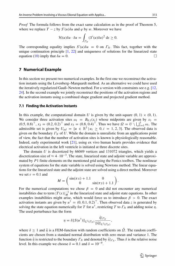
7.1 Finding the Activation Instants

In this example, the computational domain U is given by the unit-square (0, 1) × (0, 1).We consider three activation sites ωi = B0.1(xi) whose midpoints are given by x1 =(0.5, 0.8)�, x2 = (0.2, 0.2)� and x3 = (0.8, 0.4)�. Thus we have Ω = U \ ⋃3

i=1 ωi . Theadmissible set is given by Uad = {u ∈ R

3 | ui ≥ 0, i = 1, 2, 3}. The observed data isgiven on the boundary ΓN of U . While the domain is unrealistic from an applications pointof view, the fact that the number of activation sites is known is physiologically reasonable.Indeed, early experimental work [21], using ex vivo human hearts provides evidence thatelectrical activation in the left ventricle is initiated at three discrete sites.

The domain U is discretized by 66049 vertices and 131072 triangles, which yields adiscretization size of ≈ 4 · 10−3. The state, linearized state and adjoint variable are approxi-mated by P1 finite elements on the mentioned grid using the Fenics toolbox. The nonlinearsystem of equations for the state variable is solved using Newtons method. The linear equa-tions for the linearized state and the adjoint state are solved using a direct method. Moreoverwe set ε = 0.1 and

M =(sin(πx) + 1.1 0

0 sin(πy) + 1.1

)

.

For the numerical computations we chose β = 0 and did not encounter any numericalinstabilities due to term |T (x)|−1

M in the linearized state and adjoint state equations. In otherexamples instabilities might arise, which would force us to introduce β > 0. The exactactivation instants are given by u† = (0, 0.1, 0.2)�. Then observed data z is generated bysolving the state equation numerically for T for u†, restricting T to ΓN and adding noise η.The used perturbance has the form

η = δ‖S(u†)‖L2(ΓN )

η|ΓN

‖η‖L2(ΓN )

,

where δ ≥ 1 and η is a FEM-function with random coefficients on Ω . The random coeffi-cients are chosen from a standard normal distribution with zero mean and variance 1. Thefunction η is restricted to the boundary ΓN and denoted by η|ΓN

. Thus δ is the relative noiselevel. In this example we choose δ = 0.1 and δ = 10−9.


After discretization of the state and adjoint state variable by linear finite elements, theprojected Levenberg–Marquartdt Method can directly be applied. In every step of the iter-ation the matrix H(u) is calculated by solving the linearized state equation and the adjointequation for all unit vectors resulting in a 3 × 3 matrix. Thus 6 linear PDEs must be solvednumerically, see Proposition 4. Moreover the gradient of J has to be calculated by solvingthe nonlinear state equation and the adjoint state equation. So in total 8 PDEs have to besolved per iteration. The nonlinear state equation is solved by the Newton method. Sinceβ = 0 the method can be interpreted as a semi smooth Newton method. The iteration isstopped by the discrepancy principle

‖S(uKδ ) − z‖L2(ΓN ) ≤ τδ ≤ ‖S(uk) − z‖L2(ΓN ) ∀ 0 ≤ k < Kδ

with τ > 1, see for instance [7]. In our experiments we choose τ = 1.1. The parameter αk

is set to 0.1k .In the case δ = 0.1 the discrepancy criterium is satisfied after 2 iterations with a final

iterate uKδ = (0.0004, 0.0981, 0.1860)�, the state error ‖S(uKδ ) − z‖L2(ΓN ) = 0.0494 and|uKδ − u†| = 0.0141. In the case δ = 10−9 the discrepancy criterium is satisfied after5 iterations with a final iterate uKδ = (2.2 · 10−11, 0.1, 0.2)�, the state error ‖S(uKδ ) −z‖L2(ΓN ) = 4.8 · 10−10 and |uKδ − u†| = 1.1 · 10−10. So we can observe that the activationinstants are reconstructed very well relative to the noise level.

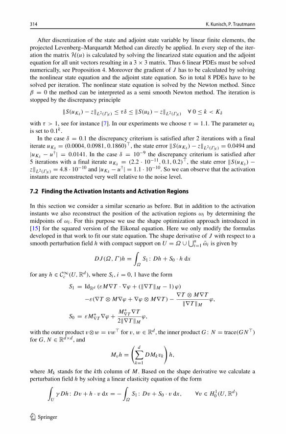
7.2 Finding the Activation Instants and Activation Regions

In this section we consider a similar scenario as before. But in addition to the activationinstants we also reconstruct the position of the activation regions ωi by determining themidpoints of ωi . For this purpose we use the shape optimization approach introduced in[15] for the squared version of the Eikonal equation. Here we only modify the formulasdeveloped in that work to fit our state equation. The shape derivative of J with respect to asmooth perturbation field h with compact support on U = Ω ∪ ⋃n

i=1 ωi is given by

DJ(Ω, Γ )h =∫

Ω

S1 : Dh + S0 · h dx

for any h ∈ C∞c (U,Rd), where Si , i = 0, 1 have the form

S1 = IdRd (εM∇T · ∇ϕ + (‖∇T ‖M − 1) ϕ)

−ε(∇T ⊗ M∇ϕ + ∇ϕ ⊗ M∇T ) − ∇T ⊗ M∇T

‖∇T ‖M

ϕ,

S0 = εM∗∇T ∇ϕ + M∗∇T ∇T

2‖∇T ‖M

ϕ,

with the outer product v⊗w = vw� for v,w ∈ Rd , the inner product G : N = trace(GN�)

for G,N ∈ Rd×d , and

Mvh =(

d∑

k=1

DMkvk

)

h,

where Mk stands for the kth column of M . Based on the shape derivative we calculate aperturbation field h by solving a linear elasticity equation of the form

∫

U

γDh : Dv + h · v dx = −∫

Ω

S1 : Dv + S0 · v dx, ∀v ∈ H 10 (U,Rd)


Table 1 Iterations and reconstruction errors for different δ

δ Kδ ‖S(XKδ , uKδ ) − z‖L2(ΓN ) d1Kδ

d2Kδ

d3Kδ

|uKδ − u†|

0.1 2 0.108 0.104 0.032 0.052 0.049

0.01 9 0.0104 0.021 0.006 0.013 0.013

0.001 52 0.001 0.003 0.001 0.008 0.005

for γ > 0 and thus h is a decent direction for J . Since we are only interested in the shiftof the midpoints xi of ωi , we average h over ωi , i = i, . . . , N , in order to get a shift of themidpoints. The proposed method is of gradient type and thus we also update the activationinstants based on the gradient calculated in Theorem 5. In particular we use a projectedgradient method.

In the specific example we choose the exact activation sites as ω†i = B0.05(xi) with

x†1 = (0.5, 0.8)�, x

†2 = (0.2, 0.3)� and x

†3 = (0.7, 0.4)�. We denote X† = [x†

1 , x†2 , x

†3 ].

The exact activation instants are given by u† = (0, 0.1, 0.2).We start the iteration at the initial points x0

1 = (0.2, 0.8)�, x02 = (0.2, 0.2)� and x0

3 =(0.8, 0.2)� and initial times u0 = (0, 0, 0). Relative noise levels are chosen to be δ =0.1, 0.01, 0.001 and the iteration is stopped using the discrepancy criterium.

In Table 1 and Fig. 1 we summarize our finding for the three noise levels δ. In particularwe document the number of iterations Kδ at which the discrepancy criterion is reached, the

Fig. 1 Top left: State error during the iteration; top right: Paths of the midpoints in U during the iteration;Bottom left: Distances between Xk and X† during the iteration; Bottom right: Error of the activation instantsduring the iteration


state error ‖S(XKδ , uKδ )−z‖L2(ΓN ), the distance between reconstructed and exact positionsdenoted by dKδ and the reconstruction error |uKδ − u†|. The reconstructed position of thethree midpoints as well as the activation instants u are given for the respective noise levelsby

XK.1 = [(0.396, 0.809), (0.22, 0.275), (0.72, 0.352)],XK.01 = [(0.496, 0.821), (0.195, 0.296), (0.711, 0.407)],XK.001 = [(0.499, 0.803), (0.201, 0.301), (0.7, 0.408)]

as well as

u.1 = (0.038, 0.113, 0.171),

u.01 = (0.011, 0.103, 0.193),

u.001 = (0.003, 0.099, 0.196).

We conclude that the positions can be reconstructed with good quality relative to thenoise level. Further tests in the noise free case showed that there is limit until which thestate error can be reduced. This is caused by discretization effects.

Acknowledgements The authors were supported by the ERC advanced grant 668998 (OCLOC) under theEU’s H2020 research program.

Funding Open access funding provided by University of Graz.

Open Access This article is licensed under a Creative Commons Attribution 4.0 International License, whichpermits use, sharing, adaptation, distribution and reproduction in any medium or format, as long as you giveappropriate credit to the original author(s) and the source, provide a link to the Creative Commons licence,and indicate if changes were made. The images or other third party material in this article are included in thearticle’s Creative Commons licence, unless indicated otherwise in a credit line to the material. If material isnot included in the article’s Creative Commons licence and your intended use is not permitted by statutoryregulation or exceeds the permitted use, you will need to obtain permission directly from the copyright holder.To view a copy of this licence, visit http://creativecommons.org/licenses/by/4.0/.

References

1. Alessandrini, G., Rondi, L., Rosset, E., Vessella, S.: The stability for the Cauchy problem for ellipticequations. Inverse Probl. 25, 123004 (2009)

2. Christof, C., Meyer, C., Walther, S., Clason, C.: Optimal control of a non-smooth semilinear ellipticequation. Math. Control Relat. Fields 8, 247–276 (2018)

3. Colli Franzone, P., Guerri, L., Rovida, S.: Wavefront propagation in an activation model of theanisotropic cardiac tissue: asymptotic analysis and numerical simulations. J. Math. Biol. 28, 121–176(1990)

4. Colli Franzone, P., Guerri, L., Tentoni, S.: Mathematical modeling of the excitation process in myocardialtissue: influence of fiber rotation on wavefront propagation and potential field. Math. Biosci. 101, 155–235 (1990)

5. Demoulin, J.C., Kulbertus, H.E.: Histopathological examination of concept of left hemiblock. Br. HeartJ. 34, 807–814 (1972)

6. Durrer, D., van Dam, R.T., Freud, G.E., Janse, M.J., Meijler, F.L., Arzbaecher, R.C.: Total excitation ofthe isolated human heart. Circulation 41, 899–912 (1970)

7. Engl, H.W., Hanke, M., Neubauer, A.: Regularization of Inverse Problems Mathematical and ItsApplications, vol. 375. Springer, Netherlands (2000)

8. Evans, L.: Partial Differential Equations. Graduate Studies in Mathematics, vol. 19. American Mathe-matical Society, Providence RI (1998)


http://creativecommons.org/licenses/by/4.0/

9. Fan, J.: On the Levenberg-Marquardt methods for convex constrained nonlinear equations. J. Ind. Manag.Optim. 9, 227–241 (2013)

10. Grandits, T., Gillette, K., Neic, A., Bayer, J., Vigmond, E., Pock, T., Plank, G.: An inverse Eikonalmethod for identifying ventricular activation sequences from epicardial activation maps. J. Comput.Phys. 419, 109700 (2020)

11. Haissaguerre, M., Vigmond, E., Stuyvers, B., Hocini, M., Bernus, O.: Ventricular arrhythmias and theHis-Purkinje system. Nat. Rev. Cardiol. 13, 155–166 (2016)

12. Kaltenbacher, B., Neubauer, A.: Convergence of projected iterative regularization methods for nonlinearproblems with smooth solutions. Inverse Probl. 22, 1105–1119 (2006)

13. Kanzow, C., Yamashita, N., Fukushima, M.: Levenberg-marquardt methods for constrained nonlinearequations with strong local convergence properties. Citeseer (2002)

14. Keener, J.P.: An eikonal-curvature equation for action potential propagation in myocardium. J. Math.Biol. 29, 629–651 (1991)

15. Kunisch, K., Neic, A., Plank, G., Trautmann, P.: Inverse localization of earliest cardiac activation sitesfrom activation maps based on the viscous Eikonal equation. J. Math. Biol. 79, 2033–2068 (2019)

16. Meyer, C., Susu, L.M.: Optimal control of nonsmooth, semilinear parabolic equations. SIAM J. ControlOptim. 55, 2206–2234 (2017)

17. Neic, A., Campos, F.O., Prassl, A.J., Niederer, S.A., Bishop, M.J., Vigmond, E.J., Plank, G.: Efficientcomputation of electrograms and ECGs in human whole heart simulations using a reaction-eikonalmodel. J. Comput. Phys. 346, 191–211 (2017)

18. Ono, N., Yamaguchi, T., Ishikawa, H., Arakawa, M., Takahashi, N., Saikawa, T., Shimada, T.: Morpho-logical varieties of the Purkinje fiber network in mammalian hearts, as revealed by light and electronmicroscopy. Arch. Hist. Cytol. 72, 139–149 (2009)

19. Pezzuto, S., Kal’avsky, P., Potse, M., Prinzen, F.W., Auricchio, A., Krause, R.: Evaluation of a rapidanisotropic model for ECG simulation. Front. Physiol. 8, 265 (2017)

20. Pullan, A.J., Tomlinson, K.A., Hunter, P.J.: A finite element method for an eikonal equation model ofmyocardial excitation wavefront propagation. SIAM. J. Appl. Math. 63, 324–350 (2002)

21. Rosenbaum, M.B., Elizari, M.V., Lazzari, J.O., Nau, G.J., Levi, R.J., Halpern, M.S.: Intraventricular tri-fascicular blocks. The syndrome of right bundle branch block with intermittent left anterior and posteriorhemiblock. Amer. Heart J. 78, 306–317 (1969)

22. Salo, M.: Unique continuation for elliptic equations. University of Jyvaskyla (2014)23. Sei, A., Symes, W.W.: Gradient calculation of the traveltime cost function without ray tracting. In: SEG

Technical Program Expanded Abstracts 1994, pp. 1351–1354. Society of Exploration Geophysicists(1994)

24. Stuck, R., Burger, M., Hohage, T.: The iteratively regularized Gauss–Newton method with convexconstraints and applications in 4Pi microscopy. Inverse Probl. 28, 015012 (2011)

25. Troianiello, G.M.: Elliptic Differential Equations and Obstacle Problems. The University Series inMathematics. Plenum Press, New York (1987)

Publisher’s Note Springer Nature remains neutral with regard to jurisdictional claims in published mapsand institutional affiliations.


Documents

An Inverse Problem Involving a Viscous Eikonal Equation