An Inventory System with Retrial Demands and Working … · International Journal of Scientific and Research Publications, Volume 4, Issue 12, December 2014 1 ISSN 2250-3153 An Inventory

International Journal of Scientific and Research Publications, Volume 4, Issue 12, December 2014 1 ISSN 2250-3153

www.ijsrp.org

An Inventory System with Retrial Demands and

Working Vacation

J. Kathiresan*, N. Anbazhagan

* and K. Jeganathan

**

*Department of Mathematics, Alagappa University, Karaikudi,India.

** Ramanujan Institute for Advanced Study in Mathematics, University of Madras, Chepauk, Chennai, India.

Abstract- This article considers a continuous review retrial

inventory system at a service facility, wherein an item demanded

by a customer is issued after performing service on the item. The

arrival time points of customers form a Poisson process. The

inventory replenished according to an ),( Qs

policy and the lead

times are assumed to follow an exponential distribution. The

demands that occur during the stock out period or the server busy

(regular or working vacation) are permitted to enter into the orbit

of infinite size. When the inventory level is zero or no demands

in the system or both, server goes to a working vacation which is

exponentially distributed. If the server is in working vacation or

the inventory level is zero, the impatience occurs in orbiting

customers, that follows an exponential distribution. The joint

probability distribution of the number of demands in the orbit,

the inventory level and the server status is obtained in the steady

state case. Some system performance measures are derived, the

long-run total expected cost rate is calculated and the results are

illustrated numerically.

Index Terms- Continuous review inventory system, ),( Qs

Policy, Positive leadtime, Retrial demand, Working vacation.

AMS Classification: 90B05, 60J27

I. INTRODUCTION

he concept of server vacation in inventory with two servers

was first introduced by Daniel and Ramanarayanan [1]. Also

they have studied an inventory system in which the server takes

rest when the level of the inventory is zero in [2]. They assumed

that the demands that occurred during stock-out period are

assumed to be lost. The inter-occurrence times between

successive demands, the lead times, and the rest times are

assumed to follow mutually independent general distributions.

Using renewal and convolution techniques they obtained the state

transition probabilities.

The various types of vacation models in queueing systems

have been widely studied in the literature. We refer the reader to

Doshi [4]. Working vacation is a kind of semi-vacation policy

that was introduced by Servi and Finn[9]. In the classical

vacation queuing models, during the vacation period the server

doesn’t continue on the original work and such policy may cause

the loss or dissatisfaction of the customers. For the working

vacation policy, the server can still work during the vacation and

may accomplish other assistant work simultaneously. So, the

working vacation more reasonable that the classical vacation in

some cases. Tien Van Do[8] studied, M/M/1 retrial queue with

working vacations. Paul Manual et al. [10] analyzed a service

facility inventory system with impatient customers. The authors

have assumed the customers arrive in Poisson fashion. The

service time, life time of items in stock and the lead time are all

assumed to be independently distributed as exponential.

The concept of retrial demands in inventory was introduced

by Artalejo et al. [3]. They have assumed Poisson demand,

exponential lead time and exponential retrial time. In that work,

the authors proceeded with an algorithmic analysis of the system.

Jeganathan et al. [5] studied a retrial inventory system with non-

preemptive priority service. Narayanan et al. [6] studied on an

),( Ss inventory policy with service time, vacation to server and

correlated lead time.

In this present paper, we address a continuous review

inventory system with Poisson demand. The server served at

different service rates (working vacation and regular), which are

exponentially distributed. When the server is busy or the

inventory level is zero, any arriving primary demands enter into

orbit. When the server is in a working vacation or the inventory

level is zero, the orbiting customer either may retry or may leave,

which is exponentially distributed. The joint probability

distribution of the inventory level, the number of customers in

the orbit and the server status is obtained in the steady state case.

Various system performance measures in the steady state are

derived and the long-run total expected cost rate is calculated and

some numerical examples.

The rest of the paper is organized as follows. In Section 2,

we describe the mathematical model. In Section 3 and 4, we

discuss the steady-state analysis of the model and some key

system performance measures respectively. In Section 5,

calculate the long-run total expected cost rate and the final

section 6, a cost function is also studied numerically.

II. MODEL DESCRIPTION

We consider a continuous review stochastic inventory

system on the replenishment policy of ),( Qs

. The basic

assumptions of this inventory model are described as follows: we

assume that the inter-arrival times of demands to a single server

station according to a Poisson process with rate 0)(>

and

demands only single unit at a time. It is assumed that there is no

waiting space in the system. The items are issued by a server to

the customer after some service time due to the service

performed on the items. When the server is busy (regular or

working vacation) or the inventory level is zero, any arriving

primary demands enter into an orbit of infinite size. The service

T

International Journal of Scientific and Research Publications, Volume 4, Issue 12, December 2014 2

ISSN 2250-3153

www.ijsrp.org

rates are b and v ()< b , when the system is in regular and

working vacation, respectively, which are exponentially

distributed. The server takes a working vacation at times when

no customers in the system or the inventory level is zero or both.

Working vacation durations are exponentially distributed with

parameter . At the completion time of the working vacation,

the server switches a regular busy ((ie) service rate from v to

b ) if there are customers (primary or retrial) in the system.

Otherwise, the server continues the working vacation. The

orbiting customers may either retry or may leave the orbit. The

leaving orbiting customers are described as impatient(reneging)

customers. If the server is in working vacation or the inventory

level is zero, the impatience occurs in orbiting customers. An

impatient customer leaves the orbit independenly after a random

time which is distributed exponentially with parameter 0)(>

.

We assume the constant retrial policy for these orbit

demands, that is probability of a repeated attempt of an orbiting

demand is independent of the number of demands in the orbit.

Retrial requests from the orbit follow an exponential distribution

with parameter 0)(>

. As the ),( Qs

replenishment policy,

when the on-hand inventory level drops to a prefixed level, say

0)(>s an order for

1)>(= ssSQ units is placed. The

positive lead time is exponentially distributed with parameter

0)(>. We assume that the inter-demand times between the

primary demands, the lead times, retrial demand times, server

regular periods and server working vacation periods are mutually

independent random variables.

Notations

ijA][ : The element / submatrix at

),( jithe position of .A

0 : Zero matrix.

I : Identity matrix.

e : A column vector of 1’s of appropriate dimension.

ij :

.0,

,=1,

otherwise

jiif

ij : ij1

)(tY:

t.at time periodregular in busy isserver the3,

t.at time periodregular in idle isserver the2,

t.at time period vacation in workingbusy isserver the1,

t.at time period vacation in working idle isserver the0,

E : ,0,0){(i

: .}0,1,2,= i ),,{( mki

: ,,1,2,=,0,1,2,= Ski 0,1,2,3}=m

III. ANALYSIS

Let )(tX

, )(tL

and )(tY

denote the number of demands in the orbit, inventory position of the commodity and the server status

at time t . From the assumptions made on the input and output processes, it can be shown that the triplet

0)),(),(),(( ttYtLtX with the state space E is a Markov process.

To determine the infinitesimal generator

))),,(),,,(((= nljmkipP,

Enljmki ),,(),,,(

of this process we use the following arguments:

Let 0=i , Sk ,1,2,=


ISSN 2250-3153

www.ijsrp.org

— any arriving primary demand takes the state of the process from ,0),( ki

to ,1),( ki

with the intensity .

— any arriving primary demand takes the state of the process from ),,( mki

to ),1,( mki

with the

intensity , 1,3=m

.

— The server changes from working vacation to regular takes the state of the process from ,1),( ki

to

,3),( ki

with the intensity .

— The completion of service from primary demand makes a transition from ,1),( ki

to 1,0),( ki

with the

intensity v .

— The completion of service from primary demand makes a transition from ,3),( ki

to 1,0),( ki

with the

intensity b .

Let 0i , 0=k

— any arriving primary demand takes the state of the process from ,0),( ki

to ,0)1,( ki

with the intensity

.

Let 1i , Sk ,1,2,=


to 1),,( mki

with the

intensity , m=0, 2.


to ),1,( mki

with the

intensity , m=1, 3.

— The server changes from working vacation to regular takes the state of the process from ),,( mki

to

2),,( mki

with the intensity , m=0, 1.

— a retrial requests takes the state of the process from ),,( mki

to 1),1,( mki

with the intensity ,

m=0, 2.

— an impatient customer takes the state of the process from ),,( mki

to ),1,( mki

with the intensity

,

m=0, 1.

— an impatient customer takes the state of the process from ,0,0)(i

to 1,0,0)( i

with the intensity

.

— The completion of service in the system makes a transition from ,1),( ki

to 1,0),( ki

with the

intensity v .

Let 1i , Sk ,2,3,=

— The completion of service in the system makes a transition from ,3),( ki

to 1,2),( ki

with the

intensity b .

— The completion of service in the system makes a transition from ,1,3)(i

to ,0,0)(i

with the intensity


ISSN 2250-3153

www.ijsrp.org

b .

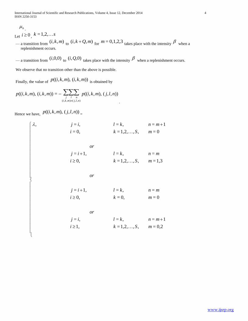
Let 0i , sk 1,2,=

— a transition from ),,( mki

to ),,( mQki

for 0,1,2,3=m

takes place with the intensity

when a

replenishment occurs.

— a transition from ,0,0)(i

to ,0),( Qi

takes place with the intensity

when a replenishment occurs.

We observe that no transition other than the above is possible.

Finally, the value of )),,(),,,(( mkimkip

is obtained by

)),,(),,,((=)),,(),,,((

),,(),,(

nljmkipmkimkipnlj

nljmki

.

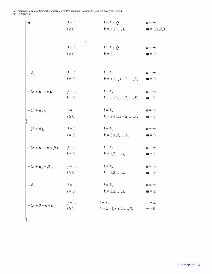
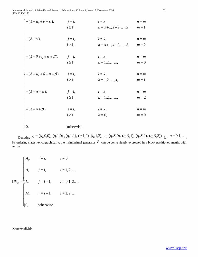
Hence we have, )),,(),,,(( nljmkip

=

0,2=,,1,2,=1,

1=,=,=

0=0,=0,

=,=1,=

1,3=,,1,2,=0,

=,=1,=

0=,,1,2,=0,=

1=,=,=,

mSki

mnklij

or

mki

mnklij

or

mSki

mnklij

or

mSki

mnklij


ISSN 2250-3153

www.ijsrp.org

00

,

,1

,1

0,1=

,,1,2,=1,

=,=1,=,

0,2=,,1,2,=1,

1=,=1,=,

0,1=,,1,2,=1,

2=,=,=

1=,,1,2,=0,=

2=,=,=,

3=1,=1,

0=1,=,=

3=,,2,=1,

1=1,=,=

3=,,1,2,=0,=

0=1,=,=,

1=,,1,2,=0,

0=1,=,=,

m

mn

k

kl

i

ij

or

m

Ski

mnklij

mSki

mnklij

mSki

mnklij

or

mSki

mnklij

mki

nklij

or

mSki

mnklij

or

mSki

nklij

mSki

nklij

b

v


ISSN 2250-3153

www.ijsrp.org

0

=

,,,2,1

,=

,1

,=),(

2=,,1,2,=0,=

=,=,=,

3=,,1,2,=0,

=,=,=),(

1=,,1,2,=0,=

=,=,=),(

0=,,0,1,2,=0,=

=,=,=),(

3=,,2,1,=0,

=,=,=),(

1=,,2,1,=0,=

=,=,=),(

0=,,2,1,=0,=

=,=,=,

0=0,=0,

=,=,=

0,1,2,3=,,1,2,=0,

=,=,=,

m

mn

Sssk

kl

i

ij

mski

mnklij

mski

mnklij

mski

mnklij

mski

mnklij

mSsski

mnklij

mSsski

mnklij

mSsski

mnklij

mki

mnQklij

or

mski

mnQklij

b

v

b

v


ISSN 2250-3153

www.ijsrp.org

otherwise0,

0=0,=1,

=,=,=),(

2=,,1,2,=1,

=,=,=),(

1=,,1,2,=1,

=,=,=),(

0=,,1,2,=1,

=,=,=),(

2=,,2,1,=1,

=,=,=),(

1=,,2,1,=1,

=,=,=),(

mki

mnklij

mski

mnklij

mski

mnklij

mski

mnklij

mSsski

mnklij

mSsski

mnklij

v

v

Denoting ,3)),(,2),,(,1),,(,0),,(,,1,3),(,1,2),(,1,1),(,,1,0)(,0,0),((= SqSqSqSqqqqqqq

for 0,1,=q

.

By ordering states lexicographically, the infinitesimal generator P can be conveniently expressed in a block partitioned matrix with

entries

otherwise0,

2,1,=1,=,

2,1,0,=1,=,

2,1,=,=,

0=,=,

=][

1

iijM

iijL

iijA

iijA

P ij

More explicitly,


ISSN 2250-3153

www.ijsrp.org

LAM

LAM

LAM

LA

P00

00

00

000

=

1

where

otherwise0,

0=,=,

,,21,=,=,

11

,,2=1,=,

0=,=),(

,,2,1=,=,

,2,1,=,=,

=][

1

4

3

1

1

iQijC

siQijC

iijJ

SiijJ

iij

siijJ

SssiijJ

A

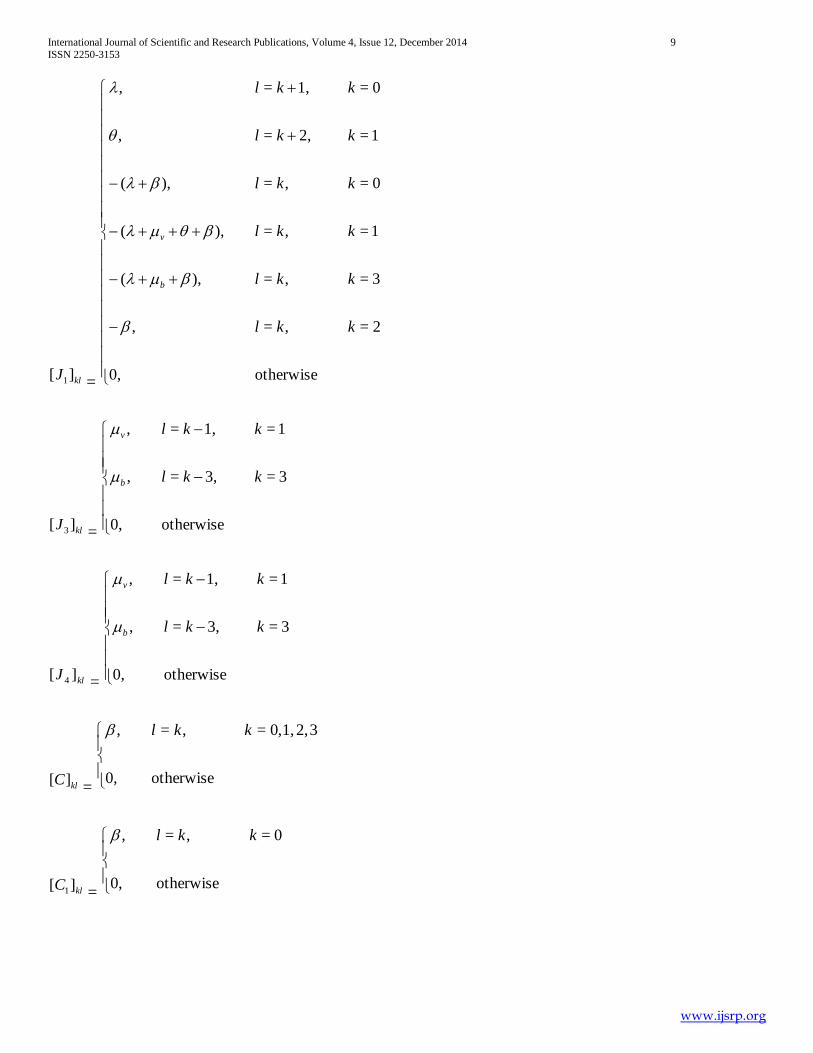
with

klJ ][

otherwise0,

3=,=),(

1=,=),(

0=,=,

1=2,=,

0=1,=,

=

kkl

kkl

kkl

kkl

kkl

b

v


ISSN 2250-3153

www.ijsrp.org

klJ ][ 1 =

otherwise0,

2=,=,

3=,=),(

1=,=),(

0=,=),(

1=2,=,

0=1,=,

kkl

kkl

kkl

kkl

kkl

kkl

b

v

klJ ][ 3 =

otherwise0,

3=3,=,

1=1,=,

kkl

kkl

b

v

klJ ][ 4 =

otherwise0,

3=3,=,

1=1,=,

kkl

kkl

b

v

klC][=

otherwise0,

32,1,,0=,=, kkl

klC ][ 1 =

otherwise0,

0=,=, kkl


ISSN 2250-3153

www.ijsrp.org

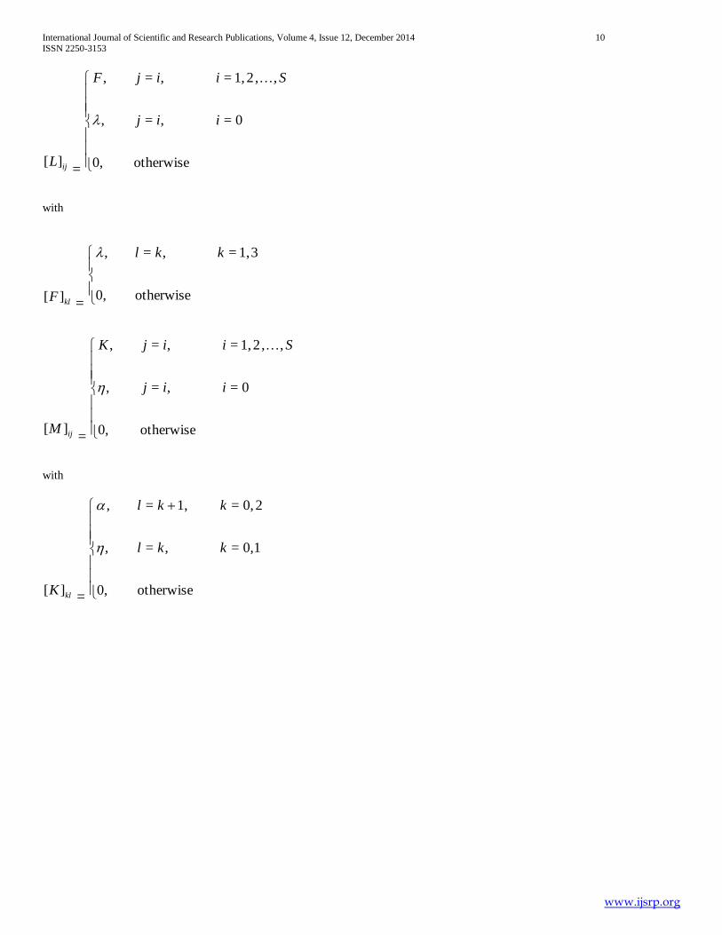
ijL][=

otherwise0,

0=,=,

,,21,=,=,

iij

SiijF

with

klF][=

otherwise0,

31,=,=, kkl

ijM ][=

otherwise0,

0=,=,

,,21,=,=,

iij

SiijK

with

klK ][=

otherwise0,

0,1=,=,

20,=1,=,

kkl

kkl


ISSN 2250-3153

www.ijsrp.org

otherwise0,

0=,=,

,2,1,=,=,

1=1,=,

,3,2,=1,=,

0=,=),(

,2,1,=,=,

,2,,1=,=,

=][

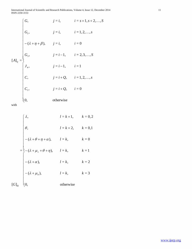
1

4

3

1

iQijC

siQijC

iijJ

SiijG

iij

siijG

SssiijG

A ij

with

klG][

otherwise0,

3=,=),(

2=,=),(

1=,=),(

0=,=),(

10,=2,=,

20,=1,=,

=

kkl

kkl

kkl

kkl

kkl

kkl

b

v


ISSN 2250-3153

www.ijsrp.org

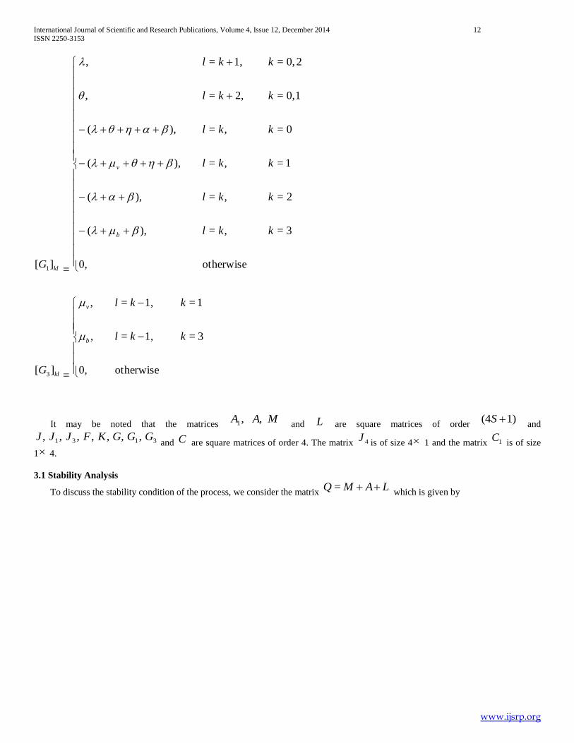
klG ][ 1 =

otherwise0,

3=,=),(

2=,=),(

1=,=),(

0=,=),(

10,=2,=,

20,=1,=,

kkl

kkl

kkl

kkl

kkl

kkl

b

v

klG ][ 3 =

otherwise0,

3=1,=,

1=1,=,

kkl

kkl

b

v

It may be noted that the matrices MAA ,,1 and L are square matrices of order

1)(4 S and

3131 ,,,,,,, GGGKFJJJ and C are square matrices of order 4. The matrix 4J

is of size 4 1 and the matrix 1C is of size

1 4.

3.1 Stability Analysis

To discuss the stability condition of the process, we consider the matrix LAMQ =

which is given by


ISSN 2250-3153

www.ijsrp.org

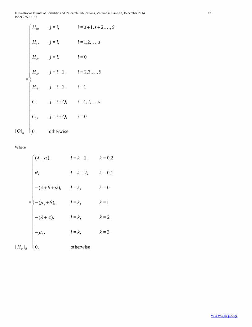
ijQ][

otherwise0,

0=,=,

,1,2,=,=,

1=1,=,

,2,3,=1,=,

0=,=,

,1,2,=,=,

,2,1,=,=,

=

1

4

3

2

1

0

iQijC

siQijC

iijH

SiijH

iijH

siijH

SssiijH

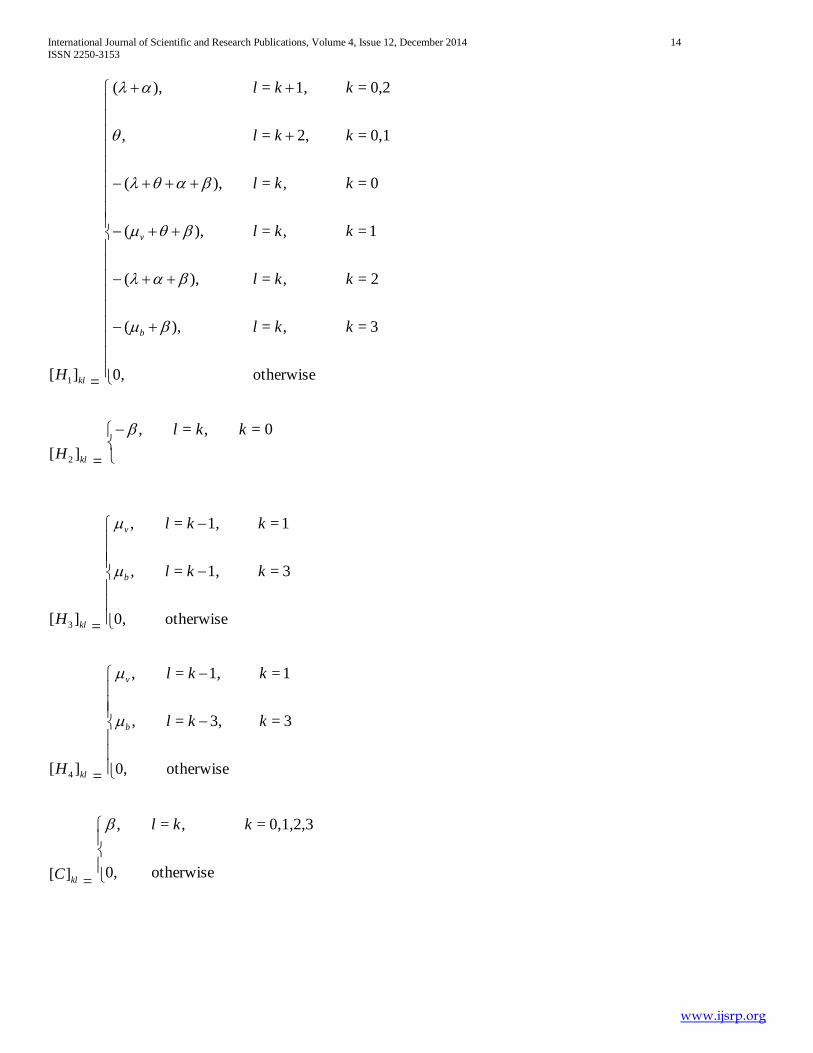
Where

klH ][ 0

otherwise0,

3=,=,

2=,=),(

1=,=),(

0=,=),(

0,1=2,=,

0,2=1,=),(

=

kkl

kkl

kkl

kkl

kkl

kkl

b

v


ISSN 2250-3153

www.ijsrp.org

klH ][ 1 =

otherwise0,

3=,=),(

2=,=),(

1=,=),(

0=,=),(

0,1=2,=,

0,2=1,=),(

kkl

kkl

kkl

kkl

kkl

kkl

b

v

klH ][ 2 = 0=,=, kkl

klH ][ 3 =

otherwise0,

3=1,=,

1=1,=,

kkl

kkl

b

v

klH ][ 4 =

otherwise0,

3=3,=,

1=1,=,

kkl

kkl

b

v

klC][=

otherwise0,

0,1,2,3=,=, kkl


ISSN 2250-3153

www.ijsrp.org

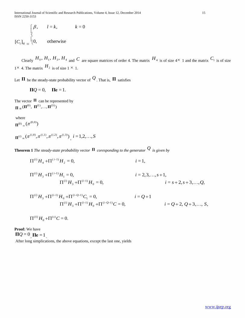
klC ][ 1 =

otherwise0,

0=,=, kkl

Clearly 4310 ,,, HHHH and C are square matrices of order 4. The matrix 4H

is of size 4 1 and the matrix 1C is of size

1 4. The matrix 2H is of size 1 1.

Let Π be the steady-state probability vector of Q

. That is, Π satisfies

1.=0,= ΠeΠQ

The vector Π can be represented by

Π =),,,( )((1)(0) S

ΠΠΠ

where

(0)Π =

)( (0,0)

)(iΠ =

),,,( ,3)(,2)(,1)(,0)( iiii ,

Si ,1,2,=

Theorem 1 The steady-state probability vector Π coresponding to the generator Q

is given by

1,=0,=2

1)(

4

)( iHH ii

1,,3,2,=0,=1

1)(

3

)( siHH ii

,,,32,=0,=0

1)(

3

)( QssiHH ii

1=0,=1

1)(

0

1)(

3

)( QiCHH Qiii

,,,32,=0,=1)(

0

1)(

3

)( SQQiCHH Qiii

0.=)(

0

)( CH sS

Proof: We have

0=QΠ, 1=Πe .

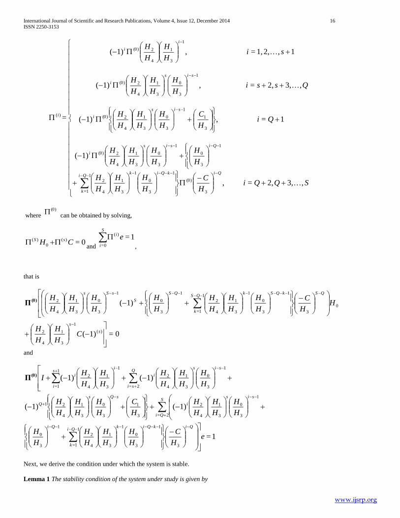
After long simplications, the above equations, except the last one, yields


ISSN 2250-3153

www.ijsrp.org

SQQiH

C

H

H

H

H

H

H

H

H

H

H

H

H

H

H

QiH

C

H

H

H

H

H

H

QssiH

H

H

H

H

H

siH

H

H

H

QikQikQi

k

Qisis

i

sis

i

sis

i

i

i

i

,3,2,=,

1)(

1=,1)(

,3,2,=,1)(

1,2,1,=,1)(

=

3

(0)

1

3

0

1

3

1

4

21

1=

1

3

0

1

3

0

3

1

4

2(0)

3

1

1

3

0

3

1

4

2(0)

1

3

0

3

1

4

2(0)

1

3

1

4

2(0)

)(

where (0)

can be obtained by solving,

0=)(

0

)( CH sS and

1=)(

0=

eiS

i

,

that is

0=1)(

1)(

)(

1

3

1

4

2

0

3

1

3

0

1

3

1

4

21

1=

1

3

0

1

3

0

3

1

4

2

s

s

QSkQSkQS

k

QS

S

sSs

CH

H

H

H

HH

C

H

H

H

H

H

H

H

H

H

H

H

H

H

H(0)Π

and

1

3

0

3

1

4

2

2=

1

3

1

4

21

1=

1)(1)(

sis

iQ

si

i

is

i H

H

H

H

H

H

H

H

H

HI(0)

Π

1

3

0

3

1

4

2

2=3

1

3

0

3

1

4

21 1)(1)(

sis

iS

Qi

sQs

Q

H

H

H

H

H

H

H

C

H

H

H

H

H

H

1=3

1

3

0

1

3

1

4

2

1

1=

1

3

0 eH

C

H

H

H

H

H

H

H

HQikQik

Qi

k

Qi

Next, we derive the condition under which the system is stable.

Lemma 1 The stability condition of the system under study is given by


ISSN 2250-3153

www.ijsrp.org

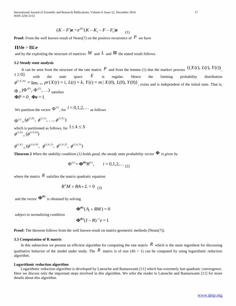
ee )(>)( 11

(0) FFKKFK (1)

Proof: From the well known result of Neuts(7) on the positive recurrence of P we have

eΠeΠ LM >

and by the exploiting the structure of matrices M and L and Π the stated result follows.

3.2 Steady state analysis

It can be seen from the structure of the rate matrix P and from the lemma (1) that the markov process ))(),(),({( tYtLtX

,

0}t with the state space E is regular. Hence the limiting probability distribution

(0)}(0),(0),|=)(,=)(,=)({lim=),,( YLXmtYktLitXprtmki

, exists and is independent of the initial state. That is,

=),,( (1)(0)

satisfies

0=PΦ , 1=Φe .

We partition the vector )(i , for

0,1,2,=i as follows

)(i =),,,( ),(,1)(,0)( Siii

which is partitioned as follows, for Sk 1 ,0)(i

=)( ,0,0)(i

),( ki=

),,,( ,3),(,2),(,1),(,0),( kikikiki

Theorem 2 When the stability condition (1) holds good, the steady state probability vector Φ is given by

0,1,2,=,= )()( iR ii (0)

Φ (2)

where the matrix R satisfies the matrix quadratic equation

0=2 LRAMR (3)

and the vector (0)

Φ is obtained by solving

0=)( 1 RMA (0)

Φ

subject to normalizing condition

1=)( 1eRI (0)

Φ

Proof: The theorem follows from the well known result on matrix-geometric methods (Neuts(7)).

3.3 Computation of R matrix

In this subsection we present an efficient algorithm for computing the rate matrix R which is the main ingredient for discussing

qualitative behavior of the model under study. The R matrix is of size (4S + 1) can be computed by using logarithmic reduction

algorithm.

Logarithmic reduction algorithm Logarithmic reduction algorithm is developed by Latouche and Ramaswami [11] which has extremely fast quadratic convergence.

Here we discuss only the important steps involved in this algorithm. We refer the reader to Latouche and Ramaswami [11] for more

details about this algorithm.


ISSN 2250-3153

www.ijsrp.org

Step 0:LAH 1)(

, MAF 1)(

, FG = , and HT =

Step 1:

FHHFU = 2= HE

EUIH 1)(

2FE

EUIF 1)(

TLGG THT

Continue Step 1: until <|||| Gee

.

Step 2:1)(= LGALR.

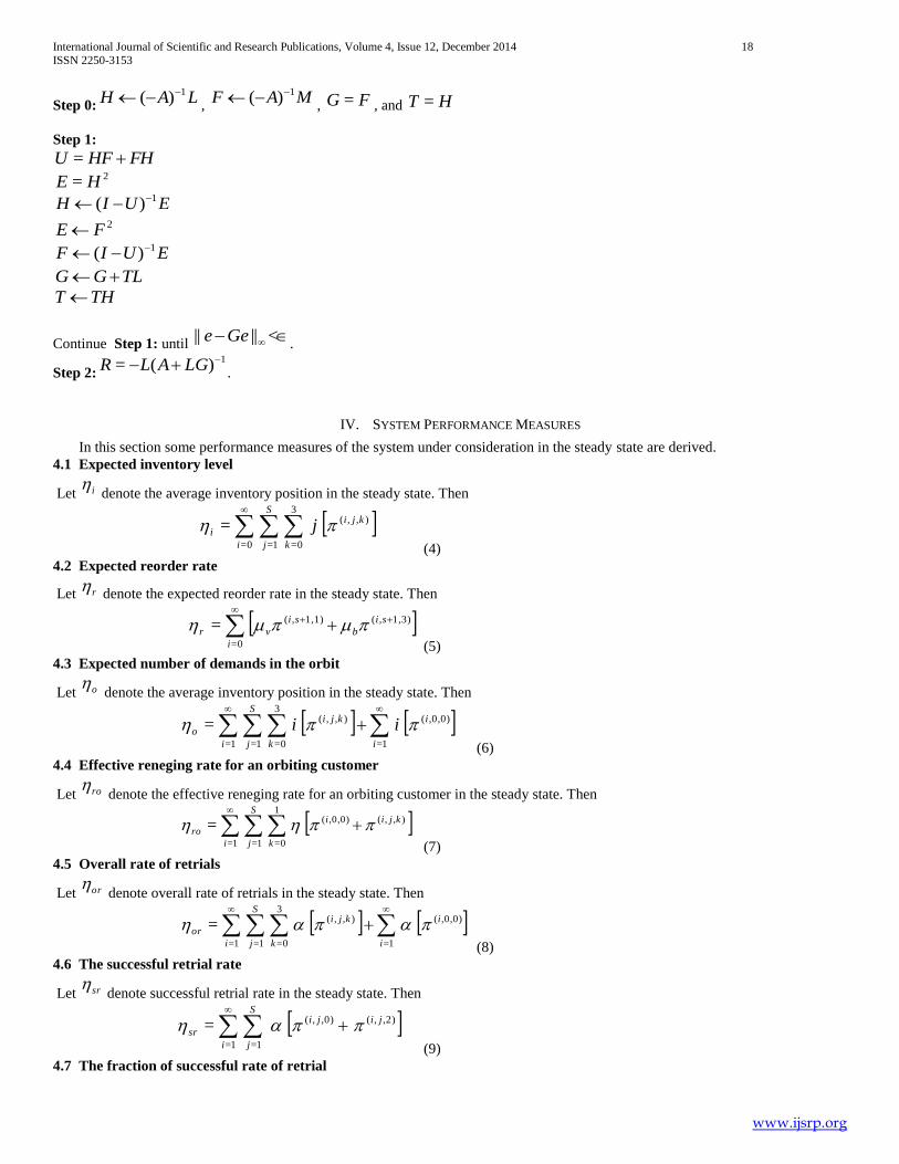
IV. SYSTEM PERFORMANCE MEASURES

In this section some performance measures of the system under consideration in the steady state are derived.

4.1 Expected inventory level

Let i denote the average inventory position in the steady state. Then

),,(3

0=1=0=

= kji

k

S

ji

i j

(4)

4.2 Expected reorder rate

Let r denote the expected reorder rate in the steady state. Then

1,3),(1,1),(

0=

=

si

b

si

v

i

r (5)

4.3 Expected number of demands in the orbit

Let o denote the average inventory position in the steady state. Then

,0,0)(

1=

),,(3

0=1=1=

= i

i

kji

k

S

ji

o ii

(6)

4.4 Effective reneging rate for an orbiting customer

Let ro denote the effective reneging rate for an orbiting customer in the steady state. Then

),,(,0,0)(1

0=1=1=

= kjii

k

S

ji

ro

(7)

4.5 Overall rate of retrials

Let or denote overall rate of retrials in the steady state. Then

,0,0)(

1=

),,(3

0=1=1=

= i

i

kji

k

S

ji

or

(8)

4.6 The successful retrial rate

Let sr denote successful retrial rate in the steady state. Then

,2),(,0),(

1=1=

= jijiS

ji

sr

(9)

4.7 The fraction of successful rate of retrial


ISSN 2250-3153

www.ijsrp.org

Let sr denote successful retrial rate in the steady state. Then

or

srfr

=

(10)

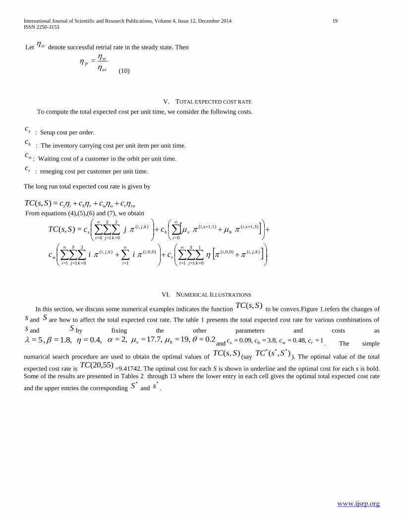
V. TOTAL EXPECTED COST RATE

To compute the total expected cost per unit time, we consider the following costs.

sc : Setup cost per order.

hc : The inventory carrying cost per unit item per unit time.

wc: Waiting cost of a customer in the orbit per unit time.

rc : reneging cost per customer per unit time.

The long run total expected cost rate is given by

rorowrhis ccccSsTC =),(

From equations (4),(5),(6) and (7), we obtain

1,3),(1,1),(

0=

),,(3

0=1=0=

=),( si

b

si

v

i

h

kji

k

S

ji

s cjcSsTC

.),,(,0,0)(1

0=1=1=

,0,0)(

1=

),,(3

0=1=1=

kjii

k

S

ji

r

i

i

kji

k

S

ji

w ciic

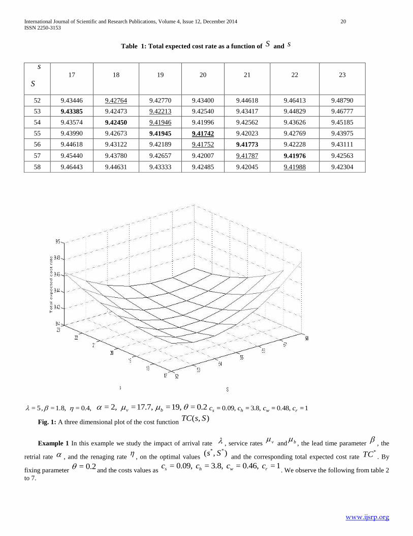
VI. NUMERICAL ILLUSTRATIONS

In this section, we discuss some numerical examples indicates the function ),( SsTC

to be convex.Figure 1.refers the changes of

s and S are how to affect the total expected cost rate. The table 1 presents the total expected cost rate for various combinations of

s and S by fixing the other parameters and costs as

4,.0=1.8,=,5= 0.2=19,=17.7,=2,= bv and1=0.48,=8,.3=0.09,= rwhs cccc

. The simple

numarical search procedure are used to obtain the optimal values of ),( SsTC

(say ),( *** SsTC

). The optimal value of the total

expected cost rate is (20,55)TC

=9.41742. The optimal cost for each S is shown in underline and the optimal cost for each s is bold.

Some of the results are presented in Tables 2 through 13 where the lower entry in each cell gives the optimal total expected cost rate

and the upper entries the corresponding *S and

*s .


ISSN 2250-3153

www.ijsrp.org

Table 1: Total expected cost rate as a function of S and s

4,.0=1.8,=,5= 0.2=19,=17.7,=2,= bv 1=0.48,=8,.3=0.09,= rwhs cccc

Fig. 1: A three dimensional plot of the cost function ),( SsTC

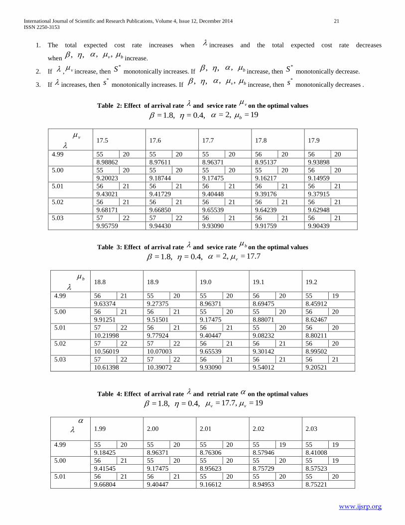
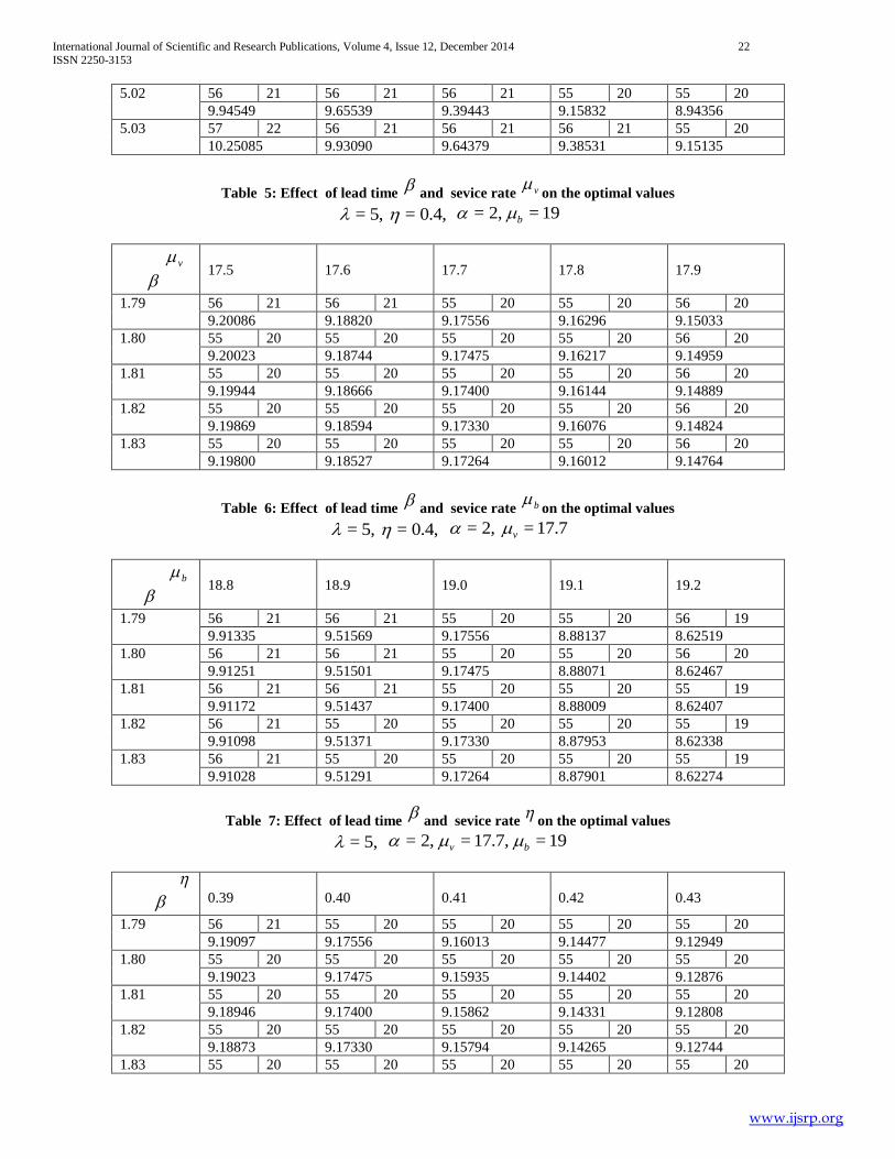
Example 1 In this example we study the impact of arrival rate , service rates v and b , the lead time parameter

, the

retrial rate , and the renaging rate

, on the optimal values ),( ** Ss

and the corresponding total expected cost rate *TC . By

fixing parameter0.2=

and the costs values as 1=0.46,=8,.3=0.09,= rwhs cccc

. We observe the following from table 2

to 7.

s

S

17

18

19

20

21

22

23

52 9.43446 9.42764 9.42770 9.43400 9.44618 9.46413 9.48790

53 9.43385 9.42473 9.42213 9.42540 9.43417 9.44829 9.46777

54 9.43574 9.42450 9.41946 9.41996 9.42562 9.43626 9.45185

55 9.43990 9.42673 9.41945 9.41742 9.42023 9.42769 9.43975

56 9.44618 9.43122 9.42189 9.41752 9.41773 9.42228 9.43111

57 9.45440 9.43780 9.42657 9.42007 9.41787 9.41976 9.42563

58 9.46443 9.44631 9.43333 9.42485 9.42045 9.41988 9.42304


ISSN 2250-3153

www.ijsrp.org

1. The total expected cost rate increases when increases and the total expected cost rate decreases

when,, bv ,,

increase.

2. If , v increase, then *S monotonically increases. If

,, b ,increase, then

*S monotonically decrease.

3. If increases, then *s monotonically increases. If

,, bv ,,increase, then

*s monotonically decreases .

Table 2: Effect of arrival rate and sevice rate v on the optimal values

4,.0=1.8,= 19=2,= b

v

17.5

17.6

17.7

17.8

17.9

4.99 55 20 55 20 55 20 56 20 56 20

8.98862 8.97611 8.96371 8.95137 9.93898

5.00 55 20 55 20 55 20 55 20 56 20

9.20023 9.18744 9.17475 9.16217 9.14959

5.01 56 21 56 21 56 21 56 21 56 21

9.43021 9.41729 9.40448 9.39176 9.37915

5.02 56 21 56 21 56 21 56 21 56 21

9.68171 9.66850 9.65539 9.64239 9.62948

5.03 57 22 57 22 56 21 56 21 56 21

9.95759 9.94430 9.93090 9.91759 9.90439

Table 3: Effect of arrival rate and sevice rate b on the optimal values

4,.0=1.8,= 7.17=2,= v

b

18.8

18.9

19.0

19.1

19.2

4.99 56 21 55 20 55 20 56 20 55 19

9.63374 9.27375 8.96371 8.69475 8.45912

5.00 56 21 56 21 55 20 55 20 56 20

9.91251 9.51501 9.17475 8.88071 8.62467

5.01 57 22 56 21 56 21 55 20 56 20

10.21998 9.77924 9.40447 9.08232 8.80211

5.02 57 22 57 22 56 21 56 21 56 20

10.56019 10.07003 9.65539 9.30142 8.99502

5.03 57 22 57 22 56 21 56 21 56 21

10.61398 10.39072 9.93090 9.54012 9.20521

Table 4: Effect of arrival rate and retrial rate on the optimal values

4,.0=1.8,= 19=7,.17= vv

1.99

2.00

2.01

2.02

2.03

4.99 55 20 55 20 55 20 55 19 55 19

9.18425 8.96371 8.76306 8.57946 8.41008

5.00 56 21 55 20 55 20 55 20 55 19

9.41545 9.17475 8.95623 8.75729 8.57523

5.01 56 21 56 21 55 20 55 20 55 20

9.66804 9.40447 9.16612 8.94953 8.75221


ISSN 2250-3153

www.ijsrp.org

5.02 56 21 56 21 56 21 55 20 55 20

9.94549 9.65539 9.39443 9.15832 8.94356

5.03 57 22 56 21 56 21 56 21 55 20

10.25085 9.93090 9.64379 9.38531 9.15135

Table 5: Effect of lead time

and sevice rate v on the optimal values

4,.0=5,= 19=2,= b

v

17.5

17.6

17.7

17.8

17.9

1.79 56 21 56 21 55 20 55 20 56 20

9.20086 9.18820 9.17556 9.16296 9.15033

1.80 55 20 55 20 55 20 55 20 56 20

9.20023 9.18744 9.17475 9.16217 9.14959

1.81 55 20 55 20 55 20 55 20 56 20

9.19944 9.18666 9.17400 9.16144 9.14889

1.82 55 20 55 20 55 20 55 20 56 20

9.19869 9.18594 9.17330 9.16076 9.14824

1.83 55 20 55 20 55 20 55 20 56 20

9.19800 9.18527 9.17264 9.16012 9.14764


and sevice rate b on the optimal values

4,.0=5,= 7.17=2,= v

b

18.8

18.9

19.0

19.1

19.2

1.79 56 21 56 21 55 20 55 20 56 19

9.91335 9.51569 9.17556 8.88137 8.62519

1.80 56 21 56 21 55 20 55 20 56 20

9.91251 9.51501 9.17475 8.88071 8.62467

1.81 56 21 56 21 55 20 55 20 55 19

9.91172 9.51437 9.17400 8.88009 8.62407

1.82 56 21 55 20 55 20 55 20 55 19

9.91098 9.51371 9.17330 8.87953 8.62338

1.83 56 21 55 20 55 20 55 20 55 19

9.91028 9.51291 9.17264 8.87901 8.62274


and sevice rate

on the optimal values

5,= 19=,7.17=2,= bv

0.39

0.40

0.41

0.42

0.43

1.79 56 21 55 20 55 20 55 20 55 20

9.19097 9.17556 9.16013 9.14477 9.12949

1.80 55 20 55 20 55 20 55 20 55 20

9.19023 9.17475 9.15935 9.14402 9.12876

1.81 55 20 55 20 55 20 55 20 55 20

9.18946 9.17400 9.15862 9.14331 9.12808

1.82 55 20 55 20 55 20 55 20 55 20

9.18873 9.17330 9.15794 9.14265 9.12744

1.83 55 20 55 20 55 20 55 20 55 20


ISSN 2250-3153

www.ijsrp.org

9.18805 9.17264 9.15730 9.14204 9.12685

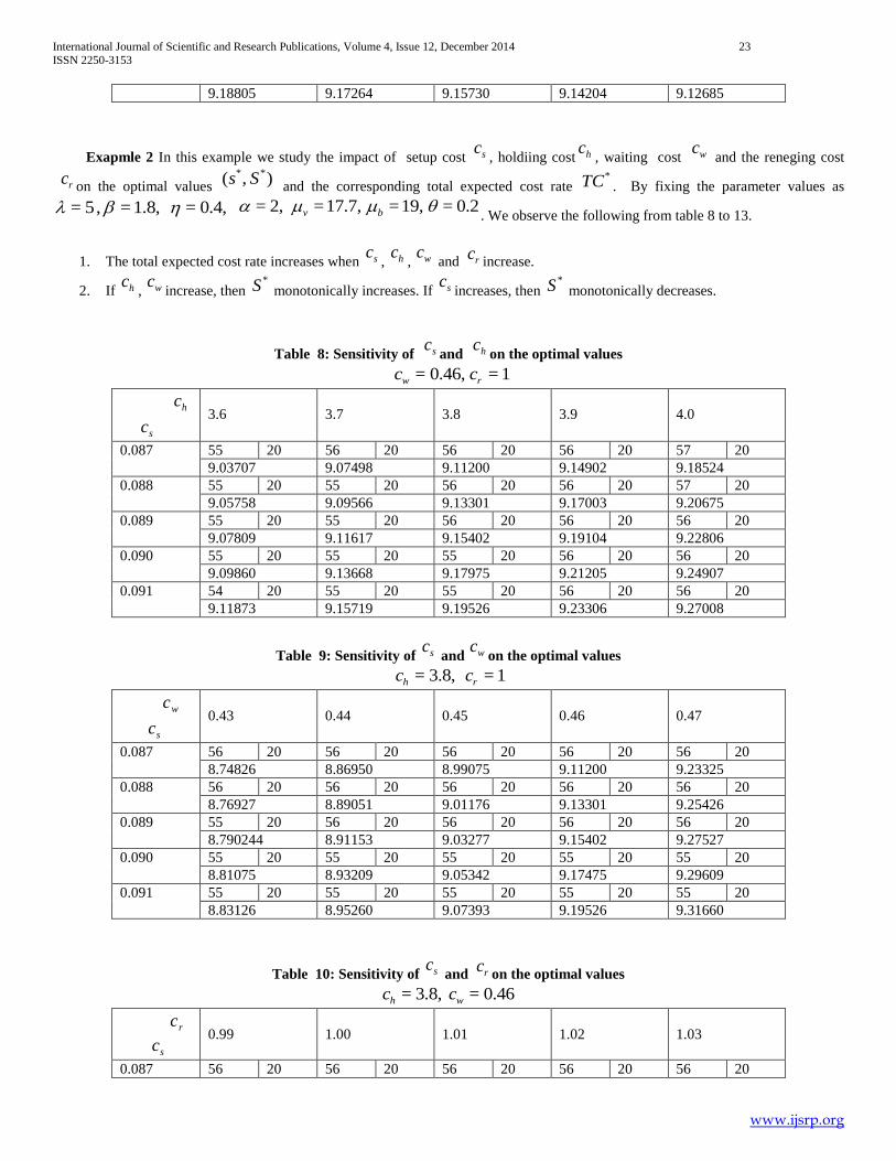
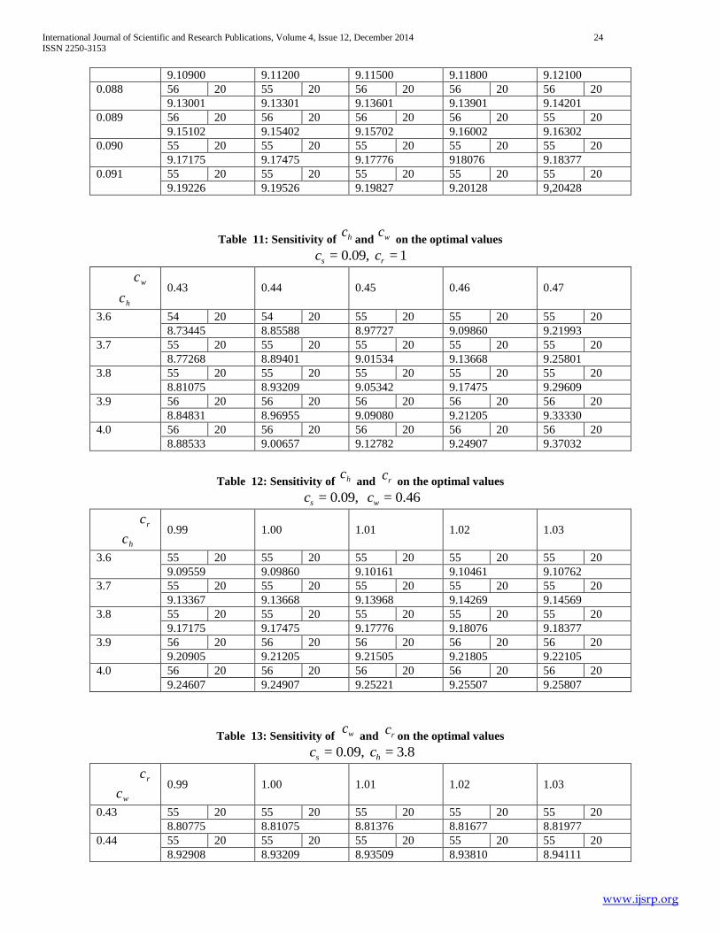
Exapmle 2 In this example we study the impact of setup cost sc, holdiing cost hc

, waiting cost wc and the reneging cost

rcon the optimal values

),( ** Ss and the corresponding total expected cost rate

*TC . By fixing the parameter values as

4,.0=1.8,=,5= 0.2=19,=17.7,=2,= bv . We observe the following from table 8 to 13.

1. The total expected cost rate increases when sc, hc

, wc and rc

increase.

2. If hc, wc

increase, then *S monotonically increases. If sc

increases, then *S monotonically decreases.

Table 8: Sensitivity of scand hc


1=0.46,= rw cc

hc

sc

3.6

3.7

3.8

3.9

4.0

0.087 55 20 56 20 56 20 56 20 57 20

9.03707 9.07498 9.11200 9.14902 9.18524

0.088 55 20 55 20 56 20 56 20 57 20

9.05758 9.09566 9.13301 9.17003 9.20675

0.089 55 20 55 20 56 20 56 20 56 20

9.07809 9.11617 9.15402 9.19104 9.22806

0.090 55 20 55 20 55 20 56 20 56 20

9.09860 9.13668 9.17975 9.21205 9.24907

0.091 54 20 55 20 55 20 56 20 56 20

9.11873 9.15719 9.19526 9.23306 9.27008

Table 9: Sensitivity of sc and wc


1=8,.3= rh cc

wc

sc

0.43

0.44

0.45

0.46

0.47

0.087 56 20 56 20 56 20 56 20 56 20

8.74826 8.86950 8.99075 9.11200 9.23325

0.088 56 20 56 20 56 20 56 20 56 20

8.76927 8.89051 9.01176 9.13301 9.25426

0.089 55 20 56 20 56 20 56 20 56 20

8.790244 8.91153 9.03277 9.15402 9.27527

0.090 55 20 55 20 55 20 55 20 55 20

8.81075 8.93209 9.05342 9.17475 9.29609

0.091 55 20 55 20 55 20 55 20 55 20

8.83126 8.95260 9.07393 9.19526 9.31660

Table 10: Sensitivity of sc and rc


0.46=8,.3= wh cc

rc

sc

0.99

1.00

1.01

1.02

1.03

0.087 56 20 56 20 56 20 56 20 56 20


ISSN 2250-3153

www.ijsrp.org

9.10900 9.11200 9.11500 9.11800 9.12100

0.088 56 20 55 20 56 20 56 20 56 20

9.13001 9.13301 9.13601 9.13901 9.14201

0.089 56 20 56 20 56 20 56 20 55 20

9.15102 9.15402 9.15702 9.16002 9.16302

0.090 55 20 55 20 55 20 55 20 55 20

9.17175 9.17475 9.17776 918076 9.18377

0.091 55 20 55 20 55 20 55 20 55 20

9.19226 9.19526 9.19827 9.20128 9,20428

Table 11: Sensitivity of hcand wc


1=09,.0= rs cc

wc

hc

0.43

0.44

0.45

0.46

0.47

3.6 54 20 54 20 55 20 55 20 55 20

8.73445 8.85588 8.97727 9.09860 9.21993

3.7 55 20 55 20 55 20 55 20 55 20

8.77268 8.89401 9.01534 9.13668 9.25801

3.8 55 20 55 20 55 20 55 20 55 20

8.81075 8.93209 9.05342 9.17475 9.29609

3.9 56 20 56 20 56 20 56 20 56 20

8.84831 8.96955 9.09080 9.21205 9.33330

4.0 56 20 56 20 56 20 56 20 56 20

8.88533 9.00657 9.12782 9.24907 9.37032

Table 12: Sensitivity of hc and rc


46.0=09,.0= ws cc

rc

hc

0.99

1.00

1.01

1.02

1.03

3.6 55 20 55 20 55 20 55 20 55 20

9.09559 9.09860 9.10161 9.10461 9.10762

3.7 55 20 55 20 55 20 55 20 55 20

9.13367 9.13668 9.13968 9.14269 9.14569

3.8 55 20 55 20 55 20 55 20 55 20

9.17175 9.17475 9.17776 9.18076 9.18377

3.9 56 20 56 20 56 20 56 20 56 20

9.20905 9.21205 9.21505 9.21805 9.22105

4.0 56 20 56 20 56 20 56 20 56 20

9.24607 9.24907 9.25221 9.25507 9.25807

Table 13: Sensitivity of wc and rc


8.3=0.09,= hs cc

rc

wc

0.99

1.00

1.01

1.02

1.03

0.43 55 20 55 20 55 20 55 20 55 20

8.80775 8.81075 8.81376 8.81677 8.81977

0.44 55 20 55 20 55 20 55 20 55 20

8.92908 8.93209 8.93509 8.93810 8.94111


ISSN 2250-3153

www.ijsrp.org

0.45 55 20 55 20 55 20 55 20 55 20

9.05041 9.05342 9.05643 9.05943 9.06244

0.46 55 20 55 20 55 20 55 20 55 20

9.17175 9.17475 9.17776 9.18076 9.18377

0.47 55 20 55 20 55 20 55 20 55 20

9.29308 9.29609 9.29909 9.30210 9.30510

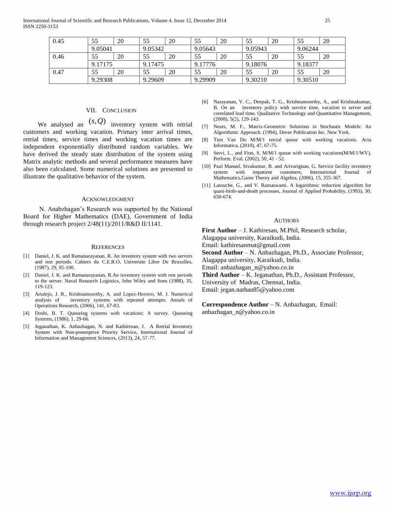
VII. CONCLUSION

We analysed an ),( Qs

inventory system with retrial

customers and working vacation. Primary inter arrival times,

retrial times, service times and working vacation times are

independent exponentially distributed random variables. We

have derived the steady state distribution of the system using

Matrix analytic methods and several performance measures have

also been calculated. Some numerical solutions are presented to

illustrate the qualitative behavior of the system.

ACKNOWLEDGMENT

N. Anabzhagan’s Research was supported by the National

Board for Higher Mathematics (DAE), Government of India

through research project 2/48(11)/2011/R&D II/1141.

REFERENCES

[1] Daniel, J. K. and Ramanarayanan, R. An inventory system with two servers and rest periods. Cahiers du C.E.R.O, Universite Libre De Bruxelles, (1987), 29, 95-100.

[2] Daniel, J. K. and Ramanarayanan, R.An inventory system with rest periods to the server. Naval Research Logistics, John Wiley and Sons (1988), 35, 119-123.

[3] Artalejo, J. R., Krishnamoorthy, A. and Lopez-Herrero, M. J. Numerical analysis of inventory systems with repeated attempts. Annals of Operations Research, (2006), 141, 67-83.

[4] Doshi, B. T. Queueing systems with vacations: A survey. Queueing Systems, (1986), 1, 29-66.

[5] Jeganathan, K. Anbazhagan, N. and Kathiresan, J. A Retrial Inventory System with Non-preemptive Priority Service, International Journal of Information and Management Sciences, (2013), 24, 57-77.

[6] Narayanan, V. C., Deepak, T. G., Krishnamoorthy, A., and Krishnakumar, B. On an inventory policy with service time, vacation to server and correlated lead time. Qualitative Technology and Quantitative Management, (2008), 5(2), 129-143.

[7] Neuts, M. F., Matrix-Geometric Solutions in Stochastic Models: An Algorithmic Approach. (1994), Dover Publication Inc. New York.

[8] Tien Van Do M/M/1 retrial queue with working vacations. Acta Informatica, (2010), 47, 67-75.

[9] Servi, L., and Finn, S. M/M/1 queue with working vacations(M/M/1/WV), Perform. Eval. (2002), 50, 41 - 52.

[10] Paul Manuel, Sivakumar, B. and Arivarignan, G. Service facility inventory system with impatient customers, International Journal of Mathematics,Game Theory and Algebra, (2006), 15, 355-367.

[11] Latouche, G., and V. Ramaswami. A logarithmic reduction algorithm for quasi-birth-and-death processes, Journal of Applied Probability, (1993), 30, 650-674.

AUTHORS

First Author – J. Kathiresan, M.Phil, Research scholar,

Alagappa university, Karaikudi, India.

Email: [email protected]

Second Author – N. Anbazhagan, Ph.D., Associate Professor,

Alagappa university, Karaikudi, India.


Third Author – K. Jeganathan, Ph.D., Assistant Professor,

University of Madras, Chennai, India.


Correspondence Author – N. Anbazhagan, Email:

[email protected]

Documents

An Inventory System with Retrial Demands and Working … · International Journal of Scientific and Research Publications, Volume 4, Issue 12, December 2014 1 ISSN 2250-3153 An Inventory