Embed Size (px)
Citation preview
AN INTRODUCTION TO THEORETICAL PROPERTIESOF FUNCTIONAL PRINCIPAL COMPONENT
ANALYSIS
Ngoc Mai Tran
Supervisor: Professor Peter G. Hall
Department of Mathematics and Statistics,
The University of Melbourne.
August 2008
Submitted in partial fulfillment of the requirements of the degree of
Bachelor of Science with Honours
Abstract
The term “functional data” refers to data where each observation is a curve, a sur-
face, or a hypersurface, as opposed to a point or a finite-dimensional vector. Func-
tional data are intrinsically infinite dimensional and measurements on the same
curve display high correlation, making assumptions of classical multivariate models
invalid. An alternative approach, functional principal components analysis (FPCA),
is used in this area as an important data analysis tool. However, presently there
are very few academic reviews that summarize the known theoretical properties
of FPCA. The purpose of this thesis is to provide a summary of some theoretical
properties of FPCA when used in functional data exploratory analysis and func-
tional linear regression. Practical issues in implementing FPCA and further topics
in functional data analysis are also discussed, however, the emphasis is given to
asymptotics and consistency results, their proofs and implications.
Acknowledgements
I would like to thank my teachers, Professors Peter Hall, Konstatin Borovkov, and
Richard Huggins, for their guidance and editing assistance.
Ngoc M. Tran, June 2008.
i
Contents
Chapter 1 Introduction 1
1.1 The concept of “functional data” . . . . . . . . . . . . . . . . . . . 1
1.2 Thesis motivation . . . . . . . . . . . . . . . . . . . . . . . . . . . . 2
1.3 A historical note . . . . . . . . . . . . . . . . . . . . . . . . . . . . 3
1.4 Definitions . . . . . . . . . . . . . . . . . . . . . . . . . . . . . . . . 4
1.4.1 FPCA from the kernel viewpoint . . . . . . . . . . . . . . . 5
1.4.2 FPCA from linear operators viewpoint . . . . . . . . . . . . 8
1.4.3 Connections between the two viewpoints . . . . . . . . . . . 10
1.4.4 FPCA and PCA . . . . . . . . . . . . . . . . . . . . . . . . 11
1.5 Estimators . . . . . . . . . . . . . . . . . . . . . . . . . . . . . . . . 13
1.6 Properties of estimators . . . . . . . . . . . . . . . . . . . . . . . . 14
1.6.1 Properties of the covariance operator . . . . . . . . . . . . . 15
1.6.2 Consistency of the eigenvalue and eigenfunction estimators . 19
1.6.3 Asymptotics of the eigenvalue and eigenfunction estimators . 21
1.6.4 Eigenspacings and confidence intervals . . . . . . . . . . . . 24
Chapter 2 Functional linear model 28
2.1 Definitions . . . . . . . . . . . . . . . . . . . . . . . . . . . . . . . . 30
2.1.1 Some background on inverse problems . . . . . . . . . . . . 31
2.1.2 Estimators . . . . . . . . . . . . . . . . . . . . . . . . . . . . 34
2.2 Regularization by truncation . . . . . . . . . . . . . . . . . . . . . . 35
2.2.1 Choice of regularization parameter . . . . . . . . . . . . . . 36
2.2.2 Estimators and relation to PCR and FPCA . . . . . . . . . 36
2.2.3 Choice of m and consistency . . . . . . . . . . . . . . . . . . 39
2.3 Mean integrated squared error . . . . . . . . . . . . . . . . . . . . . 43
2.3.1 Tikhonov regularization . . . . . . . . . . . . . . . . . . . . 44
2.3.2 MISE of the truncation method . . . . . . . . . . . . . . . . 45
2.3.3 MISE in Tikhonov regularization . . . . . . . . . . . . . . . 48
2.4 Selected topics in FLM . . . . . . . . . . . . . . . . . . . . . . . . . 49
2.4.1 Prediction . . . . . . . . . . . . . . . . . . . . . . . . . . . . 49
2.4.2 Central limit theorems . . . . . . . . . . . . . . . . . . . . . 52
ii
Chapter 3 Practical issues: sampling and smoothing 54
3.1 From discrete to functional data . . . . . . . . . . . . . . . . . . . . 54
3.2 A model for noise . . . . . . . . . . . . . . . . . . . . . . . . . . . . 57
3.3 Sparsity . . . . . . . . . . . . . . . . . . . . . . . . . . . . . . . . . 57
3.4 Smoothing with a roughness penalty . . . . . . . . . . . . . . . . . 59
3.4.1 Ridge regression . . . . . . . . . . . . . . . . . . . . . . . . . 59
3.4.2 A change in norm . . . . . . . . . . . . . . . . . . . . . . . . 60
Chapter 4 Concluding Remarks 62
4.1 A summary of the thesis . . . . . . . . . . . . . . . . . . . . . . . . 62
4.2 Further topics . . . . . . . . . . . . . . . . . . . . . . . . . . . . . . 63
iii
Chapter 1
Introduction
1.1 The concept of “functional data”
The term “functional data” refers to data where each observation is a curve, a
surface, or a hypersurface, as opposed to a point or a finite-dimensional vector. For
example, in meteology, we might want to analyze the temperature flunctuations
in Victoria. Then the temperature data collected over time at each station are
effectively producing a curve over the observed interval, with, say, 365 measurements
made over 365 days of the year. With the emergence of new technology, many
datasets contain measurements monitored over time or space, for example: a sensor
records the force applied to an object at rate 500 times per second, a computer
records position of a digital pen at rate 600 times per second [31]. Although each
measurement is discrete and could be viewed as 600 data points rather than one
curve, the collection of points possess a certain smoothness property that facilitates
the functional data interpretation.
There are several important features of functional data:
• Functional data are intrinsically infinite dimensional.
• Measurements within one curve display high correlation.
These properties render the assumptions made for multivariate analysis incorrect.
On the other hand, functional data analysis (FDA) methods exploit smoothness
of the data to avoid both the curse of dimensionality and the high correlation be-
tween measurements. In particular, the covariance function for functional data is a
smooth fixed function, while in high-dimensional multivariate data, the dimension
of covariance matrices is assumed to increase with sample size, leading to the “large
p, small n” problems [20]. Therefore, in analysis of data arising in various fields
such as longitudinal data analysis, chemometrics, econometrics, etc., the functional
data analysis viewpoint is becoming increasingly popular, since it offers an alterna-
tive way to approach high-dimensional data problems.
An important dimension reduction method for functional data is functional princi-
pal component analysis (FPCA), which is the main topic of study in this thesis. In
finite dimensional settings, principal components analysis (PCA) was first described
1
independently by Pearson in 1901 and Hotelling in 1933 as a dimension reduction
technique [22]. Finite dimensional PCA relies on expanding the data in the eigen-
basis of the covariance matrix. When extended to infinite dimension, this translates
to expanding the data in the eigenbasis of the covariance operator. FPCA reduces
the functional data to a given number of components such that the representation
is optimal in terms of its L2 accuracy. Many of the advantanges of PCA in the
finite dimensional case carry on to the infinite dimensional context, including:
• It allows analysis of variance-covariance structure, which can be difficult to
interpret otherwise.
• As an orthonormal basis expansion method, it gives the optimal basis (in the
sense that it minimizes mean L2-error).
• There is a good theoretical support for FPCA.
• The function can be broken down into “principle components”, allowing vi-
sualization of the main features of the data.
• The method extends naturally to functional linear regression, an important
topic of much practical interests.
There are several approaches to analyzing functional data. In this thesis we con-
centrate only on FPCA and its applications. Alternative treatments of fuctional
data are briefly discussed in the last chapter. Further references can be found in
books such as [31, 13].
1.2 Thesis motivation
To date, there are no books or papers summarizing the currently known proper-
ties of FPCA. Ramsay and Silverman [31] offer an applied-oriented introduction to
the topic, while asymptotics and consistency properties of estimators are scattered
over several papers by different authors in different contexts: dimension reduction
[12, 17, 18], functional linear modelling [7, 8, 16], time-series analysis [4], longi-
tudinal analysis [36, 20], to name a few. The purpose of this thesis to provide a
summary of some known theoretical properties of FPCA when used in functional
data exploratory analysis and function linear regression, as well as some interesting
theoretical issues which arise from implementing FPCA in practice. The thesis is
organized into the following chapters:
Chapter 1 introduces the theory of FPCA from both the linear operator and kernel
viewpoints. Asymptotics and consistency of estimators are discussed.
In chapter 2, an application of FPCA to the problem of functional linear model
(FLM), or functional linear regression is explored. This can be thought of as a linear
2
regression model with functional predictor and functional “slope”. This chapter
highlights the advantange of the functional view over the multivariate view in the
FLM context. The link between FLM and ill-posed inverse problems are analyzed,
and the dependence of the estimator’s properties on choice of smoothing parameter
is studied.
In practice, the observed “curve” is made up of discrete measurements. Chapter 3
investigates the theoretical impact on FPCA in translating these measurements to
the functional form, in particular, the impact on convergence rates of estimators.
Models with noise and sparse measurements are considered. The last part of chapter
3 studies some theoretical implications of smoothing with a roughness penalty.
In chapter 4, the concluding chapter, a summary is provided, and further topics
in PCA and FDA are briefly mentioned, including generalizations to multivariate
FPCA and nonparametric approaches.
1.3 A historical note
On functional data analysis
Ramsay and Silverman [31] noted that functional data have two key features: repli-
cation (taking measurements on the same subject repeatedly over different time
or different space), and smoothness (the assumption that the underlying curve has
a certain degree of smoothness). From this viewpoint, functional data analysis
touches base with a few different areas of statistics, and can even be dated back to
Gauss in 1809 and Lagrange in 1805 in the problem of estimating comet’s trajectory
[31]. Emphasis on analyzing data with replications appeared in texts on ANOVA
and longitudinal data analysis in the 1990s. Smoothness is taken into account ear-
lier, motivated by a series of papers on human growth data in 1978 by Largo (the
references can be found in [31]). Technical developments, especially in the principal
components analysis direction, were motivated by the paper published in 1982 by
Dauxois [12]. Subsequently many papers which treated functional principal com-
ponents analysis under the linear operator viewpoint were published by the French
school, with Besse [2], Cardot [7, 10], Ferraty [13], Mas [26, 25] and Bosq [4] be-
ing the main contributors (more references can be found in Ramsay and Silverman
[31]). From the 1990s onwards, with the development of technology, functional
data analysis became a fast growing area of statistics. The texts Functional Data
Analysis [31] and Nonparametric Functional Data Analysis [13] are considered to
be important texts for this topic.
3
On functional principal components analysis
In the finite dimensional setting, the first papers on principal components analysis
(PCA) were written independently by Pearson in 1901 and Hotelling in 1933. These
authors considered PCA as a dimension reduction technique [22]. Eigenanalysis for
a symmetric matrix was extended to integral operators with symmetric kernels,
leading to the Karhunen-Loeve decomposition (Karhunen, 1947, Loeve, 1945) [31],
which is an important result in the theory of FPCA. The earliest attempt to use
PCA for functional data was made in 1958 independently by Rao and Tucker,
who applied multivariate PCA without modifications to observed function values
[31]. Important asymptotic properties of PCA estimators for the infinite dimen-
sional case were first studied in 1982 by Dauxois [12]. Since then, functional PCA
(FPCA) became an important technique in functional data analysis. Many theoret-
ical development in the 1980s and 1990s came from the linear operator viewpoint,
as mentioned previously. Practical motivations, and the fact that the audience of
these papers largely consist of applied statisticians, led to more recent work which
analyze FPCA from the kernel viewpoint, see, for example, Yao et al. [36], Hall et
al. [16, 17, 20]. As we shall see, this viewpoint is beneficial in certain applications,
for example, the calculation of the kernel operator, or incorporating local smoothing
ideas, such as those used in [20, 36]. Therefore, in this thesis we shall introduce
FPCA from both perspectives. The two views are interchangable.
1.4 Definitions
Notation
Below we state some notations and definitions which will be used throughout the
thesis. Some elementary properties are stated without proofs. Details can be found
in texts on linear operators such as Weidmann [34], and in texts on stochastic
process such as Bosq [4]. These notations mainly follow that of Bosq [4].
• (Ω,A, P ): a probability space with sigma algebra A and measure P .
• L2(I) = L2(I,B, λ): the space of (class of) square-integrable functions on the
compact set I, f : I → R, (∫I f
2)1/2 < ∞. This space is a separable Hilbert
space, with inner product 〈f, g〉 :=∫I fg, and norm ‖f‖ := (
∫I f
2)1/2.
• L2(Ω) = L2(Ω,A, P ): the space of (class of) random variables Y : Ω →L2(I) such that (
∫Ω‖Y ‖2dP )1/2 < ∞. The function Y 7→ (
∫Ω‖Y ‖2dP )1/2 =∫
I E(Y 2) is a norm on L2(Ω).
• H: a separable Hilbert space. Most of the time, we work with H = L2(I).
4
• ‖K‖∞: for K a linear operator from H1 to H2, this denote the operator norm
of K, that is
‖K‖∞ = supψ∈H1,‖ψ‖=1
‖Kψ‖.
Operators K such that ‖K‖∞ < ∞ are called bounded operators. The set
of bounded linear operators from H1 to H2 is denoted B(H1,H2). Equipped
with the ‖ · ‖∞ norm, this is a Banach space.
• ‖K‖S : for K ∈ B(H1,H2), this denote the Hilbert-Schmidt norm of K, that
is, for any basis (ej)∞j=1 of H1
‖K‖S = (∞∑j=1
‖K(ej)‖2)1/2
This definition is independent of the choice of the basis (ej). Linear operators
K such that ‖K‖S < ∞ are called Hilbert-Schmidt operators. The set of
Hilbert-Schmidt operators from H1 to H2 is denoted S(H1,H2). Equipped
with the ‖ · ‖S norm, this is a Hilbert space.
• H∗: the dual space of the separable Hilbert space H. That is, it is the space
of continuous linear operators T : H → R. Now, H∗ = B(H,R) = S(H,R).
We shall use the notation ‖ · ‖ without subscript to denote the usual norm for
this space.
• x∗: for x ∈ H, x∗ denote its Riesz representation in H∗.
• ‖f‖: for f an element of L2(I), this denote the norm of f (with respect to
the usual L2-norm).
Assumptions:
For simplicity, in this thesis, we shall work with the Hilbert space L2(I) equipped
with the usual L2 inner product unless otherwise indicated. Further, we assume
that I ⊂ R. The theory of the general case holds many similarities to this case.
Some generalizations are mentioned in chapter 4.
1.4.1 FPCA from the kernel viewpoint
Let X denote a random variable X : Ω → L2(I), such that X ∈ L2(Ω). Equiva-
lently, X can be seen as a stochastic process defined on a compact set I, with finite
mean-trajectory:∫I E(X2) <∞. Define µ := E(X) to be the mean process of X.
5
Definition 1. The covariance function of X is defined to be the function K :
I × I → R, such that
K(u, v) := CovX(u), X(v) = E[X(u)− µ(u)][X(v)− µ(v)].
Assume that X has continuous and square-integrable covariance function, that is,∫ ∫K(u, v)2 du dv < ∞. Then the function K induces the kernel operator K :
L2(I) → L2(I), ψ 7→ Kψ, defined by
(Kψ)(u) =
∫IK(u, v)ψ(v) dv.
To reduce notational load, we shall use K to denote the kernel operator. The
covariance functionK would be refered to as “the (covariance) functionK”. Usually
it should be clear from the context which K is implied.
As noted, FPCA relies on an expansion of the data in terms of the eigenbasis of
K. The existence of an eigenbasis of K for L2(I) is guaranteed by Mercer’s lemma,
and the expansion of X in this basis is termed the Karhunen-Loeve expansion.
Lemma 2. Mercer’s Lemma [4](p24)
Assume that the covariance function K as defined is continuous over I2. Then
there exists an orthonormal sequence (ψj) of continuous functions in L2(I), and a
non-increasing sequence (κj) of positive numbers, such that
(Kψj)(u) = κjψj(u), u ∈ I, j ∈ N,
and moreover,
K(u, v) =∞∑j=1
κjψj(u)ψj(v), u, v ∈ I, (1.1)
where the series converges uniformly on I2. Hence
∞∑j=1
κj =
∫IK(u, u)du <∞.
Proof: A proof is given in section 1.4.2, which illustrates the link between Mercer’s
lemma and the spectral theorem for compact self-adjoint linear operators. This
important fact connects the kernel viewpoint and the linear operator viewpoint.
6
Theorem 3. Karhunen-Loeve expansion [4](p25)
Under the assumptions and notations of Mercer’s lemma, we have
X(u) = µ(u) +∞∑j=1
√κjξjψj(u), (1.2)
where ξj := 1√κj
∫X(v)ψj(v) dv is a random variable with E(ξj) = 0, and
E(ξjξk) = δj,k, j, k ∈ N,
where δj,k denote the Kronecker delta. The series (1.2) converges uniformly on Iwith respect to the L2(Ω)-norm.
Outline of proof: The key step in the proof is to change the order of integration to
obtain: EX(u)ξj = κjψj(u). Then we expand EX(u)−∑n
j=1
√κjξjψj(u)2 and
use equation (1.1) of Mercer’s lemma to obtain the uniform convergence needed.
The expectation of the eigenvalues can be checked via direct computation. 2
The key to the Karhunen-Loeve expansion, and is also one of the advantages of
the FPCA approach, is that X is broken up into orthogonal components with
uncorrelated coefficients. The eigenvalue κj can be interpreted as a measure of the
variation in X in the ψj direction. The idea of FPCA is to retain the first M terms
in the Karhunen-Loeve expansion as an approximation to X
X =M∑j=1
√κjξjψj,
and hence achieve dimension reduction. This can be seen as projecting X onto an
M -dimensional space, spans by the first M eigenfunctions of K, which are those
with the largest eigenvalues κj. This projection could be done with other basis, but
the eigenbasis (ψj) is “optimal” in the sense that it minimizes the expected error
in the M-term approximation. This lemma is stated and proved in section 1.4.3.
In the FPCA literature, there is no standard notation for the eigenvalues, eigenvec-
tors or the covariance function. Some authors denote the covariance operator by
Γ, the eigenvalues as λj, and they tend to work with the eigenprojections, which
are projections onto the space spans by the eigenfunctions, instead of the actual
eigenfunctions. Authors who approach FPCA from a kernel viewpoint such as Hall
et al. [17], Yao et al. [36], tend to call the covariance operator K, the eigenfunctions
ψj, and the eigenvalues either κj or λj. Since the kernel viewpoint was introduced
first in this thesis, our notations follow those of Hall [17].
7
For the word ‘principal component’ itself, some authors use this in reference to ψj,
others use it to refer to ξj [22]. Here we shall follow the definitions used in Dauxois
[12].
Definition 4. Let (ξj), (ψj), (κj) be defined as in the Karhunen-Loeve theorem.
Let Πj be the projection of L2(I) onto the space spans by eigenfunctions with corre-
sponding eigenvalue κj. Then the (Πj) are called eigenprojections. The (ψj) are
called the principal factors of X, the (κj) are called the principal values, and
the (ξj) are called the standardized principal components of X, and the values
(〈X,ψj〉) = (√κjξj) are called the (unstandardized) principal components of X.
Now, we shall introduce the linear operator viewpoint and study the properties of
the estimators.
1.4.2 FPCA from linear operators viewpoint
Definition 5. The covariance operator ofX is the map CX : (L2(I))∗ → L2(I),
defined by
CX(x∗) = E[x∗(X − µ)(X − µ)], x∗ ∈ (L2(I))∗.
(Recall that (L2(I))∗ stands for the space of continuous linear operators from L2(I)
to R).
This definition applies to general Banach spaces. Since L2(I) is a Hilbert space, by
the Riesz representation theorem, the covariance operator can be viewed as
CX : L2(I) → L2(I), CX(x) = E[〈X − µ, x〉(X − µ)], x ∈ L2(I).
With some computation, we recognize that this is the kernel operator K defined in
definition 1. Indeed, let x ∈ L2(I). Then CX : L2(I) → L2(I), with
CX(x)(u) = E[〈X − µ, x〉 (X − µ)(u)]
=
∫Ω
∫I(X − µ)(v, ω)x(v) dv (X − µ)(u, ω)dP (ω)
=
∫IE[(X − µ)(u)(X − µ)(v)]x(v) dv
=
∫IK(u, v)x(v) dv = Kx(u).
8
Therefore, K = CX . From now on, we shall continue to use K for the covariance
operator, in accordance with the previous section.
The following lemma states some properties of the covariance operator K. These
properties parallel those of a covariance matrix. The lemma suggests that PCA in
the functional setting relies on the same principles as in the multivariate setting.
Lemma 6. The covariance operator K is a linear, self-adjoint, positive semidefi-
nite operator.
Proof: By direct computation, using the kernel operator definition. The first
property is trivial. The second property relies on the symmetry of the covariance
function: K(u, v) = K(v, u). The third property relies on changing the order of
integration to obtain 〈Kψ,ψ〉 = E|〈X,ψ〉|2. 2
An important result for compact self-adjoint operators is the spectral theorem,
which bear close resemblance to Mercer’s lemma and the Karhunen-Loeve expan-
sion. The proof of this classical result is omitted, and can be found in [34] (p166).
Theorem 7. Spectral theorem for compact self-adjoint linear operators
(abbr.: Spectral theorem) [34](p166)
Let T be a compact self-adjoint bounded linear operator on a separable Hilbert space
H. Then there exists a sequence of real eigenvalues of T : |κ1| ≥ |κ2| ≥ · · · ≥ 0,
κj → 0 as j → ∞. Furthermore, let Πj be the orthogonal projections onto the
corresponding eigenspaces. Then the (Πj) are of finite rank, and
T =∞∑j=1
κjΠj,
where the series converges in the operator norm.
Corollary 8. There exist eigenfunctions (ψj) of T corresponding to the eigenvalues
(κj), which form an orthonormal basis for H. Further, if T is positive semidefinite,
then κj ≥ 0 for all j.
Proof: Since H is separable, if we choose a (possibly countably infinite) orthonor-
mal basis for the kernel space of T , and amalgamate them with the (ψj) in the
9
theorem to create one sequence, then this is an orthonormal basis for H.1 The
positive semidefiniteness comes from direct computation. 2
1.4.3 Connections between the two viewpoints
Authors who approach FPCA from the kernel viewpoint tend to work with the
covariance function, while those who use the operator viewpoint often work with
the covariance operator. Using the notation of tensor product spaces (see Weidmann
[34], p37), the covariance function K can be written as
covariance functionK = E(X − µ)⊗ (X − µ),
and the covariance operator can be written as
CX = operatorK = E(X − µ)∗ ⊗ (X − µ).
The duality is clear: the covariance function and covariance operator are duals
via the Riesz representation theorem. Therefore, the two views are interchangable,
which implies that results on the operator K can be easily given an interpretation in
terms of the covariance function K. Further, convergence of the covariance function
(for example, asymptotic normality) implies convergence of the covariance operator,
and vice versa.
There is a strong connection between the spectral theorem, Mercer’s lemma and
Karhunen-Loeve expansion. By the spectral theorem, (the completion of) (ψj) is
an orthonormal basis for L2(I). So for any x ∈ L2(I), Plancherel’s theorem [34]
(p38) gives
x =∞∑j=1
ψj〈x, ψj〉 =∞∑j=1
ψj
∫Ix(v)ψj(v) dv,
where the series converges in the L2-norm. This implies convergence in the L∞-
norm, which implies uniform convergence of∞∑j=1
ψj(u)
∫Ix(v)ψj(v) dv on I. The
Karhunen-Loeve theorem extends this expansion to the random variable X itself.
The uniform convergence part relies on Mercer’s lemma, which can be proved using
the spectral theorem.
Proof of Mercer’s lemma based on the spectral theorem
From lemma 6, we only need to show compactness to apply the spectral theorem
1We shall denote this amalgated sequence by (ψj) , since the newly amalgated functions arealso eigenfunctions of T with eigenvalue 0.
10
on K. This will be the case if we can show that K is a Hilbert-Schmidt operator.
Indeed: let (ei) be an orthonormal basis for H := L2(I). Then (ei ⊗ ej) is an
orthonormal basis in L2(I2), and∫I2
K2(u, v) du dv =∞∑i=1
∞∑j=1
(∫I2
K(u, v)gj(v)gi(u) du dv
)2
=∞∑j=1
∞∑i=1
(∫IKgj(u)gi(u) du
)2
=∞∑j=1
∞∑i=1
〈Kgj, gi〉 =∞∑j=1
‖Kgj‖2 <∞.
So K is a Hilbert-Schmidt operator, hence is compact. Apply the spectral theorem
to K, we obtain an orthonormal basis (ψj) for L2(I), with
(Kψj)(u) = κjψj(u), u ∈ I, j ∈ N.
Exploit the continuity of the inner product, and the fact that 〈x, y〉 = 0 for all
y ∈ L2(I) implies x = 0, we can prove that
K(u, v) =∞∑j=1
κjψj(u)ψj(v),
where the convergence is uniform on I2. Therefore
∞∑j=0
κj =
∫IK(u, u) du <∞.
This proves Mercer’s lemma. The proof highlights the relationship between the
lemma and the spectral theorem, and hence confirms the connection between the
kernel viewpoint and the linear operator viewpoint.
1.4.4 FPCA and PCA
It is worth mentioning the parallel and distinction between FPCA and PCA. In
the later case, the vector X is decomposed into components using the spectral
theorem for symmetric real matrices [22] (p13). Since symmetric real matrices are
automatically compact, this theorem is a special case of the spectral theorem stated
above. Many properties of PCA carry over to the infinite dimensional settings, for
example, “the best M -term approximation” property, noted in [12, 31].
11
Lemma 9. For any fixed M ∈ N, the first M principal factors of X satisfy
(ψi) = argmin(φi):〈φi,φj〉=δij
E
∥∥∥∥∥X −M∑i=1
〈X,φi〉φi
∥∥∥∥∥2
, (1.3)
where δij is the Kronecker’s delta.
Proof: The proof is similar to that of the finite dimensional setting. Let (φi) be
an orthonormal basis of L2(I) which give the expansion
X =∞∑i=1
〈X,φi〉φi.
By orthonormality of the (φi), the minimization problem in the right-hand side of
equation (1.3) is equivalent to maximizing E(∑M
i=1〈X,φi〉2)
subjecting to ‖φi‖ = 1
for each i.2 This can be solved by induction. Consider the case M = 1. Under the
constraint ‖φ‖ = 1, we want to maximize
E〈X,φ〉2 = E
(∫I(X − µ)φ(u) du
∫I(X − µ)(v)φ(v) dv
)= E
(∫I
∫I(X − µ)(u)(X − µ)(v)φ(v)φ(u) dv du
)=
∫I
∫IK(u, v)φ(v)φ(u) dv du
= 〈Kφ, φ〉 .
Subjecting to ‖φ‖ = 1, 〈Kφ, φ〉 is maximized when φ is the eigenfunction of K with
the largest eigenvalue, that is, φ = ψ1. An induction argument on M shows that
the basis needed consists of eigenfunctions of K arranged in a non-increasing order
of corresponding eigenvalues, which is the FPCA basis (ψi). 2
Much of the theory on the estimators of FPCA are also similar to the finite dimen-
sional case, such as the parametric O(n−1/2) convergence rates for the covariance
operator, eigenvalues and eigenfunctions, asymptotic normality, and the eigenspac-
ings problem. The distinction between the two cases only becomes clear when
compactness plays an important role. We shall analyze this in the functional linear
context regression in chapter 2.
2For this reason, the principal components basis is also sometimes derived as the orthonormalbasis which maximizes the variance in the reduced data.
12
1.5 Estimators
Suppose we are given a set X = X1, . . . , Xn of independent random functions,
identically distributed as X. Define X = 1n
∑ni=1Xi. We are interested in esti-
mating the eigenvalues (κj) and the principal factors (ψj) of X from this sample.
The principal components can be obtained by numerical evaluation of the integral∫I X(u)ψj(u) du.
Definition 10. Let X := 1n
∑ni=1Xi denote the sample mean. The empirical
approximation of K(u, v) is
K(u, v) =1
n
n∑i=1
[Xi(u)−X(u)][Xi(v)−X(v)].
This induces an integral operator, which is called the sample covariance operator
K =1
n
n∑i=1
(Xi −X)∗ ⊗ (Xi −X).
It is clear that K is also a self-adjoint, compact, positive semidefinite linear operator.
So by Mercer’s lemma, there exists an orthonormal basis (ψj) for L2(I) consisting
of eigenfunctions of K, with eigenvalues (κj), such that
K(u, v) =∞∑j=1
κjψj(u)ψj(v).
Denote the dimension of the range of K by r. Since K maps onto the space spans
by the n functions (Xi −X)ni=1 of L2(I), we have r ≤ n. Order the eigenvalues so
that κ1 ≥ κ2 ≥ · · · ≥ 0, with κj = 0 for j ≥ r + 1. Apply the spectral theorem, we
can write
K =r∑j=1
κjΠj,
where Πj corresponds to the projection onto the eigenspace with eigenvalue κj.
Complete the sequence (ψj) to obtain a complete orthonormal basis for L2(I), then
for each Xi
Xi =∞∑j=1
⟨Xi, ψj
⟩ψj.
13
In most statistical studies, such as those quoted in the reference, ψj and κj are
treated as esitmators for ψj and κj. To make this concrete, we shall state this as a
definition.
Definition 11. In this thesis, unless otherwise indicated, ψj is the eigenfunction
estimator for ψj, κj is the eigenvalue estimator for κj, and Πj is the eigenpro-
jection estimator for Πj.
Existence of the estimators
The eigenvalues are well-defined, hence so are the associated eigenprojections. The
eigenfunctions are slightly more complicated. First, since the eigenfunctions ψj are
unique up to a change of sign, without loss of generality, we can assume that ψj is
chosen such that 〈ψj, ψj〉 ≥ 0, to ensure that ψj can be viewed as an estimator of ψj
and not −ψj. Second, note that if an eigenvalue has multiplicity m > 1, then the
associated eigenspace is of dimension m > 1. Hence there is no unique eigenfunction
basis for this space: rotation of a basis would lead to new ones. Therefore, in this
thesis, for simplicity we shall primarily work with the case where eigenvalues are
distinct, that is, κ1 > κ2 > . . . ≥ 0.
Given the two conditions above, the eigenfunctions are well-defined. However, in
terms of estimations, closely spaced eigenvalues can cause problems. Specifically,
if κj − κj+1 = ε for some small ε > 0, the eigenfunctions can be so close that it is
difficult to estimate. Indeed, we have
K(ψj − ψj+1) = κj+1(ψj − ψj+1) + εψj
If ε is very small, then the function ψj − ψj+1 is only ε away from being an eigen-
function of K. Intuitively, we need large n to distinguish the two eigenfunctions ψj
and ψj+1, and this leads to slow convergence rate of the estimators ψj and ψj+1. In
the finite dimensional context, this problem is known as the eigenspacings problem,
and the effect is known as instability of the principal factors [22]. We shall discuss
this in details in the next section.
1.6 Properties of estimators
It is natural to raise the issue of the consistency and asymptotic properties of the
estimators K, ψj and κj defined above. From a practical viewpoint, these results
would allow us to derive confidence intervals and hypothesis tests. Under mild as-
sumptions, consistency results was derived by Dauxois et al. [12], using the method
14
of spectral perturbation. More specific cases, such as convergence of covariance
operators in linear processes, were studied by Mas [25]. Many models in time series
analysis, such as continuum versions of moving average and autoregressive processes
are of this type. The extra assumption on the covariance of the data (for exam-
ple, autoregressive) allows methods of operator theory to be applied effectively in
this context. Bosq [4] gives an extensive study of consistency, asymptotics and
convergence rates of FPCA estimators in autoregressive processes.
In this section we shall start with some simple but important bounds that leads to
consistency theorems. Asymptotic properties of the estimators will be summarized,
and the implications of these theorems will be analyzed. In particular, emphasis
will be given to the effects of eigenvalues spacing on convergence rates. This effect
will also be seen in the second chapter, when we look at functional linear models.
1.6.1 Properties of the covariance operator
The effect of estimating µ
In many papers in the literature, such as the work of Dauxois [12], Bosq [4], Cardot
[7], it is often assumed that E(X) = µ = 0, and that we observe (X1, . . . , Xn)
random variables, independent, identically distributed as X. This is equivalent to
approximating K(u, v) by the function
K(u, v) =1
n
n∑i=1
[Xi(u)− µ(u)][Xi(v)− µ(v)],
which induces an integral operator
K =1
n
n∑i=1
(Xi − µ)∗ ⊗ (Xi − µ).
From there, the authors deduced statements on the covariance operator K and its
eigenvalues and eigenfunctions (see, for example, Dauxois [12]).
Since we shall consider higher order terms in the theorem by Hall et al. [17], we shall
work with K instead of K. It is sometimes more convenient to prove bounds for K
by proving it for K first. The following lemma ensures that asymptotic properties
of K up to order O(n−1/2) are the same as those of K.
Lemma 12. Assume that E‖X‖4 < ∞. The term that comes from using X
instead of µ is negligible for asymptotic results of order O(n−1/2). Specifically, we
15
mean
E‖K − K‖2S = O(n−2),
which, by Jensen’s inequality, implies
E‖K − K‖S = O(n−1),
Proof: Consider
E‖K − K‖2S = E‖(X − µ)∗ ⊗ (X − µ)‖2
S = E‖X − µ‖4
where the norm on X−µ is the L2-norm in L2(I). Let Yi := Xi−µ, then the Yi are
independent, identically distributed as Y = X − µ, with E(Y ) = 0. Then, consider(n∑i=1
‖Yi‖2
)2
=
(∑i
∑j:j 6=i
〈Yi, Yj〉+∑l
‖Yl‖2
)2
=
(∑l
‖Yl‖2
)2
+ 2∑l
‖Yl‖2∑i
∑j:j 6=i
〈Yi, Yj〉+
(∑i
∑j:j 6=i
〈Yi, Yj〉
)2
.
Taking expectation, we see that
E
(∑l
‖Yl‖2
)2
= nE‖Y ‖4 + (n2 − n)(E‖Y ‖2)2.
By independence of the (Yi), we have
E
(2∑l
‖Yl‖2∑i
∑j:j 6=i
〈Yi, Yj〉
)= 0.
Again, utilizing independence of the Yi and Cauchy-Schwarz inequality, we obtain
E
(∑i
∑j:j 6=i
〈Yi, Yj〉
)2
= 2∑i
∑j:j 6=i
E〈Yi, Yj〉2 ≤ 2(n2 − n)E(‖Y ‖2)2,
This gives
E‖X − µ‖4 =1
n4E
(‖
n∑i=1
Yi‖2
)2
= O(n−2).
2
16
Now we state some important results for the estimator K. By direct computation,
we can see thatn
n− 1EK(u, v) = K(u, v). So K is asymptotically unbiased.3 An
application of the strong law of large numbers guarantees almost sure convergence
for K:
Lemma 13. Dauxois et al. [12]
Rewrite K as Kn to emphasize the dependency of K on n. Then the sequence of
random operators (Kn)n∈N converges almost surely to K in S = S(L2(I), L2(I)).
Proof: Consider the unbiased version of K, that is,
K :=1
n− 1
n∑i=1
(Xi−X)∗⊗ (Xi−X) =1
n
n∑i=1
X∗i ⊗Xi−
1
n(n− 1)
∑i
∑j:j 6=i
X∗i ⊗Xj.
Since the (Xi) are independent, (X∗i ⊗Xi) are i.i.d integrable random variable from
(Ω,A, P ). Therefore, by the strong law of large numbers (SLLN) in the separable
Hilbert space S,1
n
n∑i=1
X∗i ⊗Xi
a.s.→ E(X∗⊗X). To apply strong law of large numbers
on the second term, note that for j 6= i, Xi and Xj are independent. Therefore,
for each fixed X∗i , the SLLN applies for the sequence
1
n− 1
∑j:j 6=i
X∗i ⊗ Xj in the
separable Hilbert space X∗i ⊗ L2(I), therefore
1
n− 1
∑j:j 6=i
X∗i ⊗Xj
a.s.→ X∗i ⊗ µ.
Then apply the SLLN again for 1n
∑ni=1X
∗i ⊗ µ in the space L2(I)∗ ⊗ µ to obtain
1
n
n∑i=1
X∗i ⊗ µ
a.s.→ µ∗ ⊗ µ.
A delta-epislon argument can be set up to show that this indeed gives almost sure
convergence for the term1
n(n− 1)
∑i
∑j:j 6=i
X∗iXj to µ∗⊗µ. Combining this property
with the result for the first term, the lemma is proved. 2
3Unlike the finite dimensional case, the covariance estimator in FPCA is often taken to be thebiased term. This partly stems from the fact that many papers in literature, for example, [12, 4, 7]tend to ignore the effect of estimating µ. Ramsay and Silverman [31] (chapter 9) noted that thecorrection term does not make too much differences in practice. Therefore, we shall work withthe biased estimator K, and only refer to the unbiased version to simplify proofs.
17
Since the norm ‖ · ‖S is stronger than the norm ‖ · ‖∞, this also implies that
Kn → K almost surely in the uniform norm of S. Under the only assumption that
the covariance function of X ⊗X is bounded, we obtain O(n−1/2) convergence for
the mean.
Lemma 14. (Cardot et al.) [7]
If E‖X‖4 <∞, then
E∥∥∥K −K
∥∥∥2
∞≤ E ‖X − µ‖4
n.
Therefore,
E‖K −K‖2∞ ≤ 2E ‖X − µ‖4
n+O(n−2).
Proof: The proof for the inequality with K is a direct computation, details can be
found in Cardot [7]. To obtain the bound for K, note that
‖K −K‖2∞ ≤ 2‖K − K‖2
∞ + 2‖K −K‖2∞,
and
2‖K − K‖2∞ ≤ 2‖K − K‖2
S .
Then, by lemma 12 E‖K − K‖2S = O(n−2). The result follows. 2
Apply the central limit theorem for sequence of independent identically distributed
(i.i.d) random variables valued in a Hilbert space (see, for example, [4]), we obtain
an asymptotic result for the covariance function K.
Lemma 15. (Dauxois et al.) [12]
Let Z := n1/2(K−K) denote the scaled difference between the covariance functions
K and K. Then the function Z converges in distribution to a Gaussian process,
say, Z, with mean 0 and covariance function KZ that of the random variable (X −µ)⊗ (X − µ). Explicitly,
KZ =∑
i,j,k,l∈N
√κiκjκkκlE(ξiξjξkξl)(ψi ⊗ ψj)⊗ (ψk ⊗ ψl)
−∑i,j∈N
κiκj(ψi ⊗ ψi)⊗ (ψj ⊗ ψl)
Proof: Write
n1/2(K −K) = n1/2(K − K) + n1/2(K − K).
18
The key to this proof lies in lemma 12 and the central limit theorem (CLT) for a
sequence of independent identically distributed random variables (iid RV) valued
in a Hilbert space (see, for example, [4]). To set up the machinery, take the tensor
product of the Hilbert space L2(I) with itself to obtain L2(I)⊗ L2(I). This space
is isomorphic to L2(I2). Let (X − µ) ⊗ (X − µ) : Ω → L2(I2) denote the random
variable mapping to L2(I2), whose images are functions of the form (u, v) 7→ (X −µ)⊗ (X − µ)(u, v) = (X − µ)(u)(X − µ)(v). Note that the covariance function K
can be written as
K = E(X − µ)⊗ (X − µ).
and the estimator K can be written as
K =1
n
n∑i=1
(Xi − µ)⊗ (Xi − µ).
Now, the space L2(I2) is also a Hilbert space. Then, by the CLT for a sequence of
iid RV mapping to a Hilbert space,
n1/2(K −K) = n−1/2
n∑i=1
(Xi ⊗Xi − E(X ⊗X)) −→ N (0, C)
where C is the covariance function of (X − µ) ⊗ (X − µ), which is E(X − µ) ⊗(X − µ)⊗ (X − µ)⊗ (X − µ).Lemma 12 gives
E‖K − K‖2 = O(n−2)
hence
E‖n1/2(K − K)‖2 = O(n−1),
that is, n1/2(K−K) converges in mean-squared to 0, which implies that it converges
to 0 in distribution. Hence the term n1/2(K − K) makes a negligible contribution
in convergence in distribution of Z. The result follows. 2
1.6.2 Consistency of the eigenvalue and eigenfunction esti-
mators
In one of the first papers on the theoretical properties of FPCA, Dauxois et al. [12]
used the methods of spectral perturbation to analyzed the properties of κj, Πj and
ψj. The idea is this: if we have a linear operator T , and another linear operator T
which is a small deviation from T , we want to know how much does the spectrum
of T deviate from that of T . This is known as the spectral perturbation problem
[24], which is one of the areas of perturbation theory for linear operators, and is
19
a large and developed field of mathematics. Therefore, in this section, we shall
not give details of Dauxois’ results, but only attempt to mention the geometric
interpretation of the proof where appropriate, and concentrate on analyzing the
statistical implications.
Firstly, we consider an important result which gives a bound on the eigenvalues and
eigenfunctions in terms of the operator norm of the covariance operator. Versions
of this result appeared in Dauxois et al. [12] and Bosq [4].
Proposition 16. (Bosq) [4], lemma 4.1, 4.3
supj≥1
|κj − κj| ≤∥∥∥K −K
∥∥∥∞.
If the eigenvalues are all distinct (that is, κ1 > κ2 > · · · ), then
∥∥∥ψj − ψj
∥∥∥ ≤ 2√
2
ρj
∥∥∥K −K∥∥∥∞
where ρj := min(κj − κj+1, κj−1 − κj) if j ≥ 2, and ρ1 = κ1 − κ2.
Proof: The results come from direct computation. As a consequence of theorem 7,
κj = ‖K −j−1∑i=1
Πi‖∞ = minl∈Lj−1
‖K − l‖∞,
where Lj−1 is the space of bounded operators from L2(I) to L2(I) such that the
range of l is of dimension j − 1 or less. A similar identity holds for κj. The result
for the eigenvalues follows by the triangle inequality. For the eigenfunctions, we
expand Kψj − κjψj and ψj − ψj in terms of the (ψi)i∈N basis, and use the bound
on the eigenvalues to obtain the result needed. Details of both proofs can be found
in Bosq [4], lemma 4.1, 4.3 2
Proposition 16 has several important implications. Firstly, coupled with lemma 13,
it is clear that the eigenvalue estimators κj converges almost surely and uniformly
to their true values. This allows the tools of perturbation theory to be applied to
obtain convergence results for the eigenfunctions and eigenprojections. The idea
is to consider the general case where κj ∈ C. Then (κj) are singularities of the
resolvent function: R : C → C, R(z) := 1K−zI , where I is the identity operator.
Write κj as κnj to emphasize its dependence on n. Then as n → ∞, the sequence
of eigenvalue estimators (κnj )n∈N converges to the singularity κj. Since convergence
for all j is at uniform rate, after some large enough n, each sequence(κnj)
lies
almost surely in a circle Cεj of radius ε, and the circles for different j are disjoint.
20
Therefore, functional calculus methods can be applied to the resolvent function (for
example, integrating around a closed contour inside Cεj), and from there bounds
can be obtained. This is the underlying idea of spectral perturbation analysis, and
is used repeatedly by Dauxois et al. [12], Cardot [7] to obtain convergence and
central limit theorems for estimators. We state below a result for convergence of
the eigenvalues and eigenprojections, obtained from this method by Dauxois.
Lemma 17. (Dauxois et al.) [12]
Write the eigenprojection estimator Πj and the eigenfunction estimator ψj as Πnj
and ψnj repsectively, to emphasize its dependence on n. For each j ∈ N and each
n ∈ N, Πnj is a random variable from (Ω,A, P ) into (S,BS). The sequence (Πn
j )n∈N
converges to Πj in S almost surely. If the eigenvalue κj is of multiplicity 1, then ψnjis a well-defined random variable from (Ω,A, P ) into L2(I). The sequence (ψnj )n∈N
converges to ψj in L2(I) almost surely. The subset of Ω on which the eigenvalues,
the eigenfunctions and the eigenprojections converge is the same as the subset of Ω
on which Kn converges to K.
Another important implication of proposition 16 is: if E‖X‖4 <∞, then by lemma
14, we have mean-squared convergence at the “parametric” rate O(n−1) for both
the eigenvalue and the eigenfunction estimators, despite the infinite dimensional-
ity of the data. Proposition 16 also illustrate the eigenspacings problem: at order
O(n−1/2), eigenspacings affects the convergence of the eigenfunction estimators ψj,
but not that of the eigenvalue estimators κj. We shall see when analyze a theorem
by Hall and Hosseini-Nasab [17] that at higher order, eigenspacings also affects the
convergence of the eigenvalue estimators. In other words, eigenfunction estimators
are more sensitive to variations in the covariance operator, making them more dif-
ficult to estimate in “worse” conditions, such as the case of sparse data, which will
be analyzed in chapter 3.
1.6.3 Asymptotics of the eigenvalue and eigenfunction es-
timators
Given the close connection between the eigenfunctions, eigenvalues and the covari-
ance operator, we would expect asymptotically the distribution of κj and ψj to be
related to the distribution of Z (recall, Z was defined in lemma 15). Note that
Z itself is the kernel of an operator, say, K, in S. Then K is a Gaussian random
21
element in S, with covariance function that of (X − µ)∗ ⊗ (X − µ). That is,
KK =∑
i,j,k,l∈N
√κiκjκkκlE(ξiξjξkξl)(ψ
∗i ⊗ ψj)⊗ (ψ∗k ⊗ ψl)
−∑i,j∈N
κiκj(ψ∗i ⊗ ψi)⊗ (ψ∗j ⊗ ψl) (1.4)
This covariance function induces a covariance operator, which we shall also denote
by KK to reduce notational load. Then we have the following result.
Proposition 18. Asymptotic distribution of the eigenvalues and eigen-
functions (Dauxois et al.) [12]
Assume that the eigenvalues are all distinct. For each j ∈ N, the asymptotic dis-
tribution of n1/2(κnj − κj) is the distribution of the eigenvalue of ΠjKΠj, which is a
Gaussian random variable with mean zero. Define the operator
Sj :=∑l:l 6=j
(κj − κl)−1ψ∗l ⊗ ψl.
Then for each j ∈ N, n1/2(ψnj − ψj) converges in distribution to the zero-mean
gaussian random variable SjK(ψj).
The proof, which is based on spectral perturbation and convergence of measures, is
omitted and can be found in Dauxois et al. [12]. To illustrate the implications of
the theorem, we shall consider the case where the eigenvalues are all distinct, and
X is a Gaussian process. This example comes from the results in Dauxois et al.
[12].
Example 19. (Dauxois et al.) [12]
Suppose that X is a Gaussian process. Then the standardized principal components
(ξi) are not only uncorrelated, but also independent and distributed asN(0, 1). This
implies
E(ξiξjξkξl) =
3 if i = j = k = l
1 if i = j, k = l, i 6= k; or i = k, j = l, i 6= j; or i = l, j = k, i 6= j
0 otherwise.
22
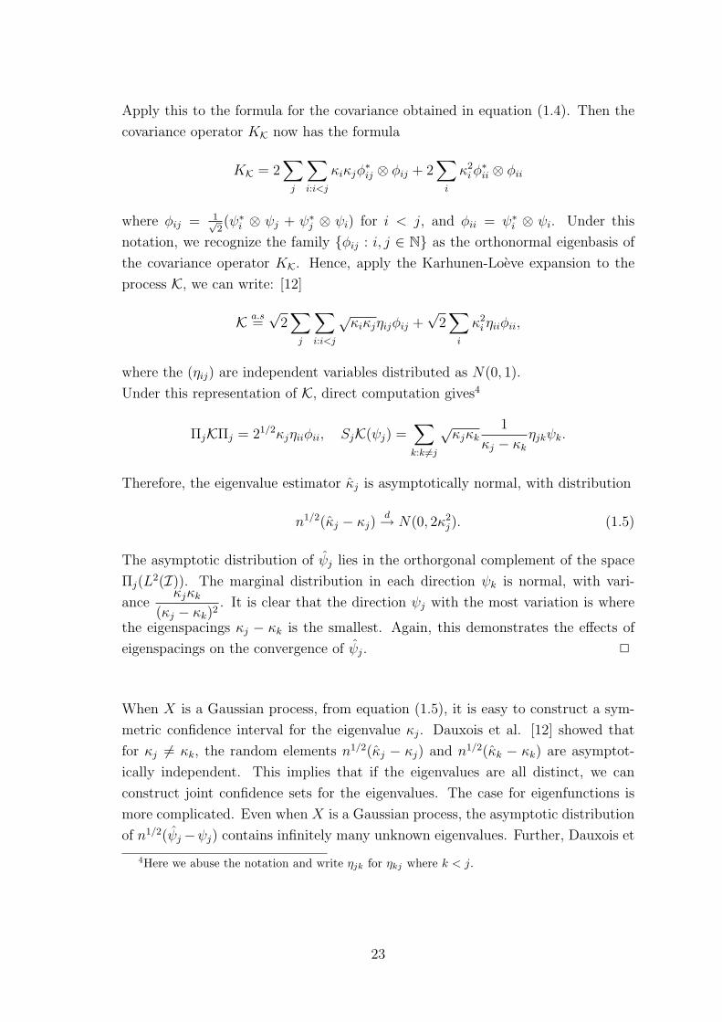
Apply this to the formula for the covariance obtained in equation (1.4). Then the
covariance operator KK now has the formula
KK = 2∑j
∑i:i<j
κiκjφ∗ij ⊗ φij + 2
∑i
κ2iφ
∗ii ⊗ φii
where φij = 1√2(ψ∗i ⊗ ψj + ψ∗j ⊗ ψi) for i < j, and φii = ψ∗i ⊗ ψi. Under this
notation, we recognize the family φij : i, j ∈ N as the orthonormal eigenbasis of
the covariance operator KK. Hence, apply the Karhunen-Loeve expansion to the
process K, we can write: [12]
K a.s=√
2∑j
∑i:i<j
√κiκjηijφij +
√2∑i
κ2i ηiiφii,
where the (ηij) are independent variables distributed as N(0, 1).
Under this representation of K, direct computation gives4
ΠjKΠj = 21/2κjηiiφii, SjK(ψj) =∑k:k 6=j
√κjκk
1
κj − κkηjkψk.
Therefore, the eigenvalue estimator κj is asymptotically normal, with distribution
n1/2(κj − κj)d→ N(0, 2κ2
j). (1.5)
The asymptotic distribution of ψj lies in the orthorgonal complement of the space
Πj(L2(I)). The marginal distribution in each direction ψk is normal, with vari-
anceκjκk
(κj − κk)2. It is clear that the direction ψj with the most variation is where
the eigenspacings κj − κk is the smallest. Again, this demonstrates the effects of
eigenspacings on the convergence of ψj. 2
When X is a Gaussian process, from equation (1.5), it is easy to construct a sym-
metric confidence interval for the eigenvalue κj. Dauxois et al. [12] showed that
for κj 6= κk, the random elements n1/2(κj − κj) and n1/2(κk − κk) are asymptot-
ically independent. This implies that if the eigenvalues are all distinct, we can
construct joint confidence sets for the eigenvalues. The case for eigenfunctions is
more complicated. Even when X is a Gaussian process, the asymptotic distribution
of n1/2(ψj−ψj) contains infinitely many unknown eigenvalues. Further, Dauxois et
4Here we abuse the notation and write ηjk for ηkj where k < j.
23
al. [12] showed that for ψj 6= ψk, n1/2(ψj−ψj) and n1/2(ψk−ψk) are not asymptot-
ically independent. Therefore, constructing joint confidence sets from proposition
18 is difficult.
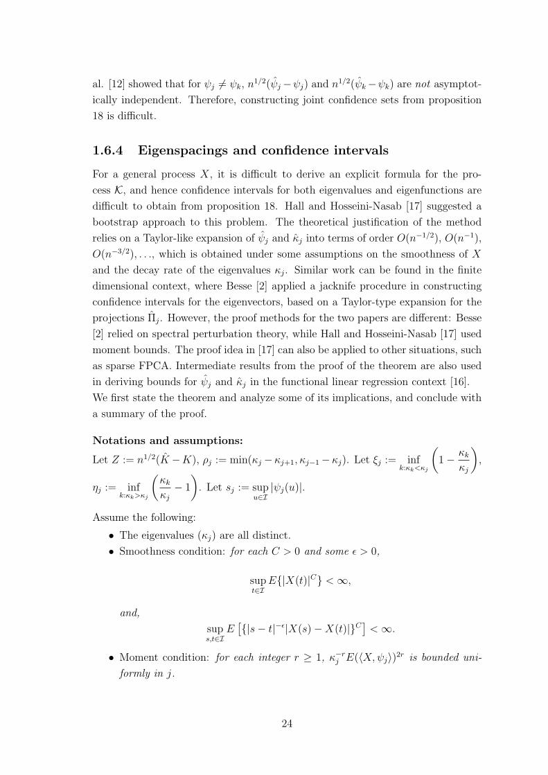
1.6.4 Eigenspacings and confidence intervals
For a general process X, it is difficult to derive an explicit formula for the pro-
cess K, and hence confidence intervals for both eigenvalues and eigenfunctions are
difficult to obtain from proposition 18. Hall and Hosseini-Nasab [17] suggested a
bootstrap approach to this problem. The theoretical justification of the method
relies on a Taylor-like expansion of ψj and κj into terms of order O(n−1/2), O(n−1),
O(n−3/2), . . ., which is obtained under some assumptions on the smoothness of X
and the decay rate of the eigenvalues κj. Similar work can be found in the finite
dimensional context, where Besse [2] applied a jacknife procedure in constructing
confidence intervals for the eigenvectors, based on a Taylor-type expansion for the
projections Πj. However, the proof methods for the two papers are different: Besse
[2] relied on spectral perturbation theory, while Hall and Hosseini-Nasab [17] used
moment bounds. The proof idea in [17] can also be applied to other situations, such
as sparse FPCA. Intermediate results from the proof of the theorem are also used
in deriving bounds for ψj and κj in the functional linear regression context [16].
We first state the theorem and analyze some of its implications, and conclude with
a summary of the proof.
Notations and assumptions:
Let Z := n1/2(K −K), ρj := min(κj −κj+1, κj−1−κj). Let ξj := infk:κk<κj
(1− κk
κj
),
ηj := infk:κk>κj
(κkκj− 1
). Let sj := sup
u∈I|ψj(u)|.
Assume the following:
• The eigenvalues (κj) are all distinct.
• Smoothness condition: for each C > 0 and some ε > 0,
supt∈I
E|X(t)|C <∞,
and,
sups,t∈I
E[|s− t|−ε|X(s)−X(t)|C
]<∞.
• Moment condition: for each integer r ≥ 1, κ−rj E(〈X,ψj〉)2r is bounded uni-
formly in j.
24
Call these assumptions “condition C”. The smoothness condition requires that the
process X has all moments finite for all t and the sample paths have some Holder-
type continuity. This is a strong smoothness assumption on X, much stronger than
the existence of 4th order moment assumption, for example. Hall and Hosseini-
Nasab [18] pointed out that if X is left-continuous (or right-continuous) at each
point with probability 1, and if that smoothness assumption hold, then for each
C > 0
E(‖K −K‖CS ) < (some constant)× n−C/2.
By the reverse triangle inequality, this implies that ‖K‖ is bounded in all orders.
This is a quite strong assumption on the covariance operator. The moment condition
ensures that all moments of the squared standardized principal components are
uniformly bounded in j. A process that satisfies this property is the Gaussian
process, for example.
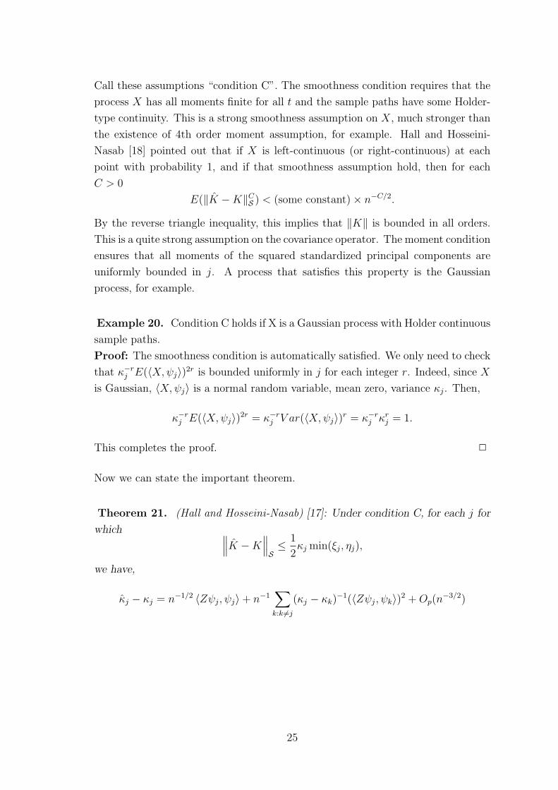
Example 20. Condition C holds if X is a Gaussian process with Holder continuous
sample paths.
Proof: The smoothness condition is automatically satisfied. We only need to check
that κ−rj E(〈X,ψj〉)2r is bounded uniformly in j for each integer r. Indeed, since X
is Gaussian, 〈X,ψj〉 is a normal random variable, mean zero, variance κj. Then,
κ−rj E(〈X,ψj〉)2r = κ−rj V ar(〈X,ψj〉)r = κ−rj κrj = 1.
This completes the proof. 2
Now we can state the important theorem.
Theorem 21. (Hall and Hosseini-Nasab) [17]: Under condition C, for each j for
which ∥∥∥K −K∥∥∥S≤ 1
2κj min(ξj, ηj),
we have,
κj − κj = n−1/2 〈Zψj, ψj〉+ n−1∑k:k 6=j
(κj − κk)−1(〈Zψj, ψk〉)2 +Op(n
−3/2)
25
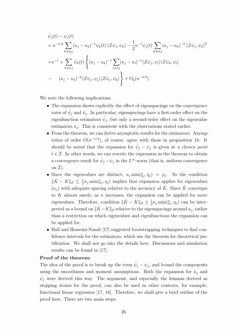
ψj(t)− ψj(t)
= n−1/2∑k:k 6=j
(κj − κk)−1ψk(t) 〈Zψj, ψk〉 −
1
2n−1ψj(t)
∑k:k 6=j
(κj − κk)−2 〈Zψj, ψk〉2
+n−1 ×∑k:k 6=j
ψk(t)
(κj − κk)
−1∑l:l 6=j
(κj − κl)−1〈Zψj, ψl〉〈Zψk, ψl〉
− (κj − κk)−2〈Zψj, ψj〉〈Zψj, ψk〉
+Op(n
−3/2).
We note the following implications.
• The expansion shows explicitly the effect of eigenspacings on the convergence
rates of ψj and κj. In particular, eigenspacings have a first-order effect on the
eigenfunction estimators ψj, but only a second-order effect on the eigenvalue
estimators κj. This is consistent with the observations stated earlier.
• From the theorem, we can derive asymptotic results for the estimators. Asymp-
totics of order O(n−1/2), of course, agree with those in proposition 18. It
should be noted that the expansion for ψj − ψj is given at a chosen point
t ∈ I. In other words, we can rewrite the expression in the theorem to obtain
a convergence result for ψj−ψj in the L∞-norm (that is, uniform convergence
on I).
• Since the eigenvalues are distinct, κj min(ξj, ηj) = ρj. So the condition
‖K − K‖S ≤ 12κj min(ξj, ηj) implies that expansion applies for eigenvalues
(κj) with adequate spacing relative to the accuracy of K. Since K converges
to K almost surely, as n increases, the expansion can be applied for more
eigenvalues. Therefore, condition ‖K − K‖S ≤ 12κj min(ξj, ηj) can be inter-
preted as a bound on ‖K−K‖S relative to the eigenspacings around κj, rather
than a restriction on which eigenvalues and eigenfunctions the expansion can
be applied for.
• Hall and Hosseini-Nasab [17] suggested bootstrapping techniques to find con-
fidence intervals for the estimators, which use the theorem for theoretical jus-
tification. We shall not go into the details here. Discussions and simulation
results can be found in [17].
Proof of the theorem:
The idea of the proof is to break up the term ψj − ψj, and bound the components
using the smoothness and moment assumptions. Both the expansion for κj and
ψj were derived this way. The argument, and especially the lemmas derived as
stepping stones for the proof, can also be used in other contexts, for example,
functional linear regression [17, 16]. Therefore, we shall give a brief outline of the
proof here. There are two main steps.
26
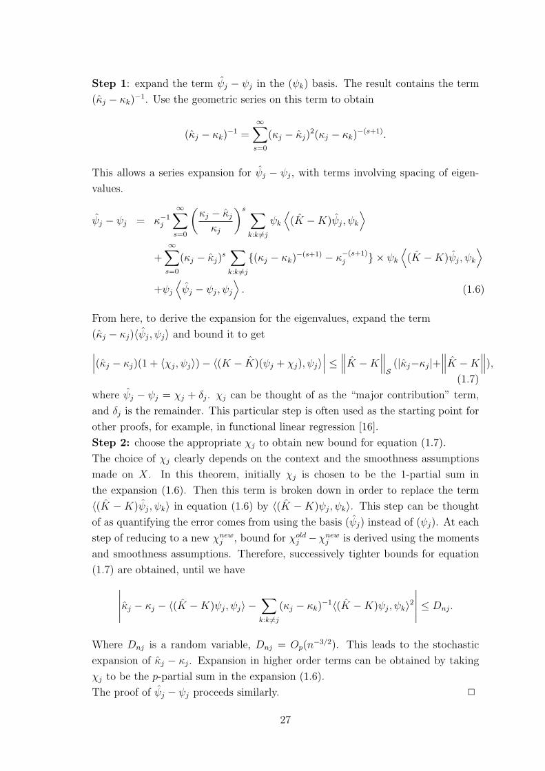
Step 1: expand the term ψj − ψj in the (ψk) basis. The result contains the term
(κj − κk)−1. Use the geometric series on this term to obtain
(κj − κk)−1 =
∞∑s=0
(κj − κj)2(κj − κk)
−(s+1).
This allows a series expansion for ψj − ψj, with terms involving spacing of eigen-
values.
ψj − ψj = κ−1j
∞∑s=0
(κj − κjκj
)s ∑k:k 6=j
ψk
⟨(K −K)ψj, ψk
⟩+
∞∑s=0
(κj − κj)s∑k:k 6=j
(κj − κk)−(s+1) − κ
−(s+1)j × ψk
⟨(K −K)ψj, ψk
⟩+ψj
⟨ψj − ψj, ψj
⟩. (1.6)
From here, to derive the expansion for the eigenvalues, expand the term
(κj − κj)〈ψj, ψj〉 and bound it to get∣∣∣(κj − κj)(1 + 〈χj, ψj〉)− 〈(K − K)(ψj + χj), ψj〉∣∣∣ ≤ ∥∥∥K −K
∥∥∥S
(|κj−κj|+∥∥∥K −K
∥∥∥),(1.7)
where ψj − ψj = χj + δj. χj can be thought of as the “major contribution” term,
and δj is the remainder. This particular step is often used as the starting point for
other proofs, for example, in functional linear regression [16].
Step 2: choose the appropriate χj to obtain new bound for equation (1.7).
The choice of χj clearly depends on the context and the smoothness assumptions
made on X. In this theorem, initially χj is chosen to be the 1-partial sum in
the expansion (1.6). Then this term is broken down in order to replace the term
〈(K −K)ψj, ψk〉 in equation (1.6) by 〈(K −K)ψj, ψk〉. This step can be thought
of as quantifying the error comes from using the basis (ψj) instead of (ψj). At each
step of reducing to a new χnewj , bound for χoldj −χnewj is derived using the moments
and smoothness assumptions. Therefore, successively tighter bounds for equation
(1.7) are obtained, until we have∣∣∣∣∣κj − κj − 〈(K −K)ψj, ψj〉 −∑k:k 6=j
(κj − κk)−1〈(K −K)ψj, ψk〉2
∣∣∣∣∣ ≤ Dnj.
Where Dnj is a random variable, Dnj = Op(n−3/2). This leads to the stochastic
expansion of κj − κj. Expansion in higher order terms can be obtained by taking
χj to be the p-partial sum in the expansion (1.6).
The proof of ψj − ψj proceeds similarly. 2
27
Chapter 2
Functional linear model
Functional linear model (FLM), also known as functional linear regression, is a lin-
ear regression model where the response is scalar, but the predictor and the slope
are functions. Such models arise in practical applications in the field of chemo-
metrics [13], climatology [31] and neurology [11] to name a few. Since the slope
“parameter” is a function, in a nonparametric context, it is determined by an in-
finite number of unknowns. This raises an ill-posed problem for the multivariate
approach, where each measurement is treated as an observation. To take a concrete
example, consider the Canadian weather dataset of Ramsay and Silverman [31].
The predictor contains 35 × 365 measurements, Xij, of temperature recorded at
the ith station on the jth day. The response Yi is the total annual precipitation at
weather station i. A naive multivariate approach would be to set up the model
Yi = β0 +365∑j=1
Xijβj + εi, i = 1, 2, . . . , 35.
This is a system of 35 equations with 366 unknowns, so there are infinitely many
sets of solutions, all giving perfect prediction of the observed data. The problem
is more than a simple overfit: Ramsay and Silverman [31] analyzed a model with
monthly average temperature rather than daily variations, reducing the problem
to 13 unknowns. The authors showed that the problem raises statistical questions
beyond the formal difficulty of fitting an under-determined model. And clearly,
taking measurements on a sparser grid might not be the most effective dimension
reduction technique.
This is where the functional viewpoint demonstrates its advantages over the multi-
variate alternative. Due to its wide applications, functional linear modelling is one
of the areas of functional data analysis that has undergone the most development
since the late 90s, both theoretically and practically. Approaches to the problem
include dimension reduction using FPCA [7, 17, 16], spline and basis function ex-
pansion [8, 31], nonparametric kernel methods [13, 1]. Generalizations of functional
28
linear model and hypothesis testing were also investigated by various researchers.
A list of references can be found in the book by Ramsay and Silverman [31].
There are more appropriate multivariate techniques which deal with highly corre-
lated data better than the naive approach mentioned above. A variety of multivari-
ate tools were developed by the chemometrics community. Major methods consist
of partial least squares (PLS), principal components regression (PCR) and ridge
regression (RR). The theoretical properties of these tools were summarized in 1993
by Frank and Friedmann [14]. However, it was noted by several authors (Marx, Eil-
ers, Hastie, Mallows, amongst others) that a functional technique which takes into
account the functional nature of the data is more beneficial than the multivariate
approaches mentioned above [8]. The contexts considered by these authors are often
practice-based, in the sense that the function X is assumed to be observed as a col-
lection of discrete points on a grid. Therefore, the main approaches proposed often
include smoothing methods, such as B-spline smoothing. Computational aspects of
these methods were discussed in detail in Ramsay and Silverman [31], chapter 15.
Some theoretical discussions can be found in Cardot et al. [8]. As mentioned, more
recent developments include nonparametric approaches, and FLM is an active area
of research.
In this chapter, we shall only study the theoretical properties of the functional lin-
ear model under the assumption that the whole curve X is observed. Furthermore,
we shall study FLM as an application of FPCA, therefore, only methods based
on FPCA are discussed in details. We take an operator viewpoint, where FLM is
shown to be equivalent to an ill-posed inverse problem. Treatment of such prob-
lems often involve regularization. Mathematical background on inverse problems,
including regularization and definition of estimators are discussed in section 1. In
section 2, we study one of the most common technique of regularization in this
field, regularization by truncation, which is also a FPCA-based technique. The link
between this method and the finite-dimensional technique PCR is briefly discussed.
The choice of the smoothing parameter m and consistency are the main points of
focus. In section 3, we shall compare the performance of mean integrated squared
error (MISE) of the estimator from the FPCA truncation method versus that ob-
tained by Tikhonov regularization. We shall analyze results of Hall and Horowitz
[16], which shows that under certain assumptions, both estimators attain the same
optimal rate, though the Tikhonov one is more robust against eigenspacing.
In practice, the problem of estimating the “slope” is arguably not as important as
the prediction problem of estimating E(Y |X = x). While the former is a nonpara-
metric problem, Hall and Horowitz [16] showed that it is possible to attain O(n−1/2)
29
rate in mean-squared convergence for the predictor. Cardot [10] also noted this dif-
ference while deriving central limit theorems in the two contexts. These points shall
be discussed in details in the last section.
2.1 Definitions
This introduction follows that of Cardot et al. [7, 10] and Hall and Horowitz [16],
with Groetsch [15] as the main reference to the theoretical background on inverse
problems.
Let Y : Ω → R be a real-valued random variable, EY 2 <∞. Let X = (X(t), t ∈ I)
be a continuous time process defined on the same space (Ω,A, P ), with finite mean
trajectory∫I E(X2) <∞. Let µY := E(Y ), µX := E(X).
Definition 22. A functional linear regression of Y on X is the problem of
finding the solution b ∈ L2(I) which solves the minimization problem:
infβ∈L2(I)
EY − µY − 〈β,X − µX〉2. (2.1)
Some simple calculation shows that a solution b exists and is unique if and only if
b satisfies
Y − µY = 〈b,X − µX〉+ ε, (2.2)
where ε : Ω → R is a real random variable with mean zero, variance σ2, and is
uncorrelated to X, that is: Eε(X − µX) = 0. Next, we introduce a measure of
the relationship between X and Y .
Definition 23. Define the cross-covariance function of Y and X to be the
function g ∈ I such that
g = E(Y − µY )(X − µX).
g induces a kernel operator G, called the cross-covariance operator of Y and X,
G : L2(I) → R, and
G = E(Y − µY )(X − µX)∗.
LetK denote the covariance operator ofX, with eigenvalues (κj) and eigenfunctions
30
(ψj). It is easy to see that b satisfies equation (2.2) if and only if it also solves
Kb = g. (2.3)
The problem of estimating b from K and g is known as an inverse problem in
operator theory [15]. The idea is: given the observed data g and the operator K,
we want to find the parameter b which gave rise to it. In this thesis, we shall work
with equation (2.3) more often than equation (2.1) or (2.2) to make use of the rich
theory behind inverse problems. We first introduce some mathematical background
on this topic.
2.1.1 Some background on inverse problems
Let D(T ), R(T ), N(T ) denote the domain, range and nullspace of an operator T ,
respectively. Let H⊥ denote the orthorgonal complement of the space H. Existence
and uniqueness of a solution to equation (2.3) is summarized by Picard’s condition.
Theorem 24. Picard’s condition [15] (p78)
Let gj denote 〈g, ψj〉, bj denote 〈b, ψj〉. Equation (2.3) has a solution if and only if
g ∈ R(K) and for all κj 6= 0,∞∑j=1
κ−2j g2
j <∞. (2.4)
Further, a solution has the form
b =∞∑j=1
κ−1j gjψj + ϕ,
where ϕ ∈ N(K).
Note that the condition g ∈ R(K) is equivalent to Y lies in R(X − µX)∗ ⊕R(X − µX)∗⊥, which is a dense subset of the space of measurable functions from
Ω to R with finite second moment. Therefore, we can require in our model that
g ∈ R(K). To ensure uniqueness, we need to assume that N(K) = 0. Note that
this is equivalent to having all eigenvalues κj of K greater than 0. The theory for
the case of N(K) 6= 0 can be dealt with by considering least-squares minimal-
norm solution to equation (2.3), but in the end the same formula for the estimator
is produced, so we shall not consider this case here. Further, if N(K) 6= 0, the
least-squares minimal norm for equation (2.3) does not solve equation (2.2), which
is the original problem of motivation. We summarize the discussion in this section
below.
31
Remark 25. From now on, we assume that g ∈ R(K), g and K satisfy the
Picard’s condition in equation (2.4), and that N(K) = 0. Then there exists a
unique solution to equation (2.3), which is also the unique solution to equation (2.2).
Under these assumptions, we see that K has an inverse K† which maps g to b. That
is,
K† : R(K) ⊆ L2(I) → L2(I), K†(g) :=∞∑j=1
κ−1j gjψj.
Existence and uniqueness is not enough for an inverse problem to be called “well-
posed”. For this, we need another condition: stability of the solution. This means
a small perturbation in g would correspond to a small perturbation in b, in other
words, b varies continuously with g.
Definition 26. [27] The operator equation (2.3) is said to be well-posed relative
to the space L2(I) if for each g, equation (2.3) has a unique solution which depends
continuously on g. Otherwise, it is said to be ill-posed.
The continuous dependent on g implies that K† is continuous. Note that R(K) =
N(K)⊥ (see, for example, [15] p77). So the assumption N(K) = 0 implies that
R(K) = D(K†) is dense in L2(I), that is, K† is a densely defined operator. The
following proposition gives conditions under which such an operator is bounded, or
equivalently, continuous.
Proposition 27. [15] (p81)
K† is a closed densely defined linear operator which is bounded if and only if R(K)
is closed. For K a compact operator, R(K) is closed if and only if R(K) is finite
dimensional.
Since we assumed N(K) = 0 to obtain uniqueness, R(K) cannot be finite di-
mensional. Therefore, proposition 27 implies that the unique solution given by
bj = κ−1j gj is unstable, as illustrated in the following example from Groetsch [15]:
Example 28. (Groetsch) [15] (p83)
Write
K†(g) =∞∑j=1
κ−1j gjψj =
∞∑j=1
κ−1j 〈g, ψj〉ψj.
32
Consider an ε-size perturbation in g: gε := g + εκj. Then, as j →∞,
‖K†g −K†gε‖ = κ−1j ε→∞.
This shows the idea of a small perturbation in g leads to a large (in this case,
infinity-size) variation in b.
Note that unlike the finite-dimensional case, equation (2.3) gives an ill-posed prob-
lem in the infinite dimensional context. Here the distinction lies in the fact that
compact operators in a infinite-dimension space behave differently from those in
finite-dimension one, as pointed out by proposition 27. This is where the theory of
“functional” settings diverge from that of its multivariate parallel.
A survey of methods for ill-posed inverse problems can be found in Groetsch [15].
Here we only consider in details the method based on principal components, which
is regularization by truncation. Later in this thesis, we consider Tikhonov regular-
ization to compare the performance of estimators. The main idea of most methods
for ill-posed problems is regularization: to exchange an exact, but unstable solu-
tion of the ill-posed problem (2.3) for a less exact, but stable solution of a near-by
well-posed problem. This somewhat resembles the variance-bias tradeoff. The well-
posed problem can be written in the general form
Kmbm = gm (2.5)
where m is a regularization parameter such that as m approaches some limit value,
such as infinity, gm → g, Km → K. Then for each fixed m, we obtain an inverse
K‡m such that K‡
m → K†. Hence (bm) = (K‡mgm) is a sequence of stable estimators
that approach b.
Note that stability of the solution to the well-posed problem in equation (2.5) means
that bm varies continuously with perturbations in gm, not with perturbations in g.
Therefore, the choice of m is a delicate matter: as m → ∞, bm is a more accurate
estimator for b, but equation (2.5) mirrors the instability of the original equation
(2.3), hence bm varies more for small perturbations in g. The optimal choice of m is
based on the level of error we expect to see in g, and this is called a regular choice.
Definition 29. Regular choice of m [15] (p87)
Let gδ be an element in L2(I) such that ‖g − gδ‖ ≤ δ. Let bm and bδm be the
solutions to equation (2.5) with values gm and gδm respectively. A choice m = m(δ)
33
is said to lead to a regular algorithm for the ill-posed problem in equation (2.3) if
m(δ) →∞ and bδm(δ) → b as δ → 0.
The choice of m to ensure regularity play an important role in determining conver-
gence rate of the estimator, and this shall be our focus point of discussion. Finally,
note that unlike usual inverse problems in literature (for example, those studied
in Groetsch [15]), the operator K is unknown and needs to be estimated from the
data. Therefore, we shall consider the general idea of estimation under regulariza-
tion next.
2.1.2 Estimators
Assume that we observed n independent random data points (Xi, Yi), identically
distributed as (X,Y ). Let X :=1
n
n∑i=1
Xi, Y :=1
n
n∑i=1
Yi.
Definition 30. The estimator for the covariance function g is
g :=1
n
n∑i=1
(Xi −X)⊗ (Yi − Y ).
Let gj denote 〈g, ψj〉. Let K denote the estimator for K as in chapter 1. Then, if b
is the solution of equation (2.3), direct computation shows that b satisfies
Kb = g + U, U :=1
n
n∑i=1
(Xi −X)(εi − ε).
As noted in chapter 1, the range of K is at most of dimension n. So for a fixed n,
no inverse of K exists, therefore we cannot approximate b by b defined as Kb = g.
However, consider the empirical approximation to the regularization equation (2.5),
that is, the equation
Kmbm = gm.
Provided that m is chosen such that gm ∈ R(Km), this equation is well-posed.
Therefore, to find an estimator for b, the idea is to construct a sequence of inverse
K‡m as approximations to K‡
m, with m = m(n) chosen such that K‡m → K† as
n → ∞. Then each K‡m yields a bm, and as n → ∞, bm → b. The scheme can be
34
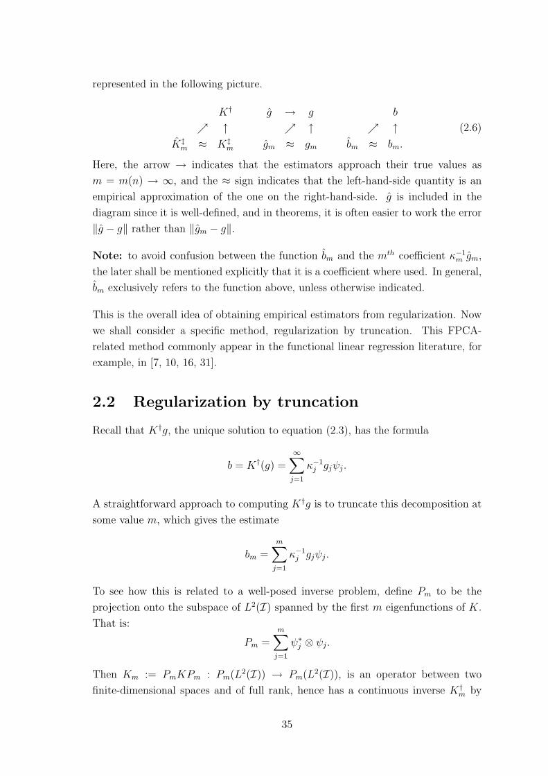
represented in the following picture.
K† g → g b
↑ ↑ ↑K‡m ≈ K‡
m gm ≈ gm bm ≈ bm.
(2.6)
Here, the arrow → indicates that the estimators approach their true values as
m = m(n) → ∞, and the ≈ sign indicates that the left-hand-side quantity is an
empirical approximation of the one on the right-hand-side. g is included in the
diagram since it is well-defined, and in theorems, it is often easier to work the error
‖g − g‖ rather than ‖gm − g‖.
Note: to avoid confusion between the function bm and the mth coefficient κ−1m gm,
the later shall be mentioned explicitly that it is a coefficient where used. In general,
bm exclusively refers to the function above, unless otherwise indicated.
This is the overall idea of obtaining empirical estimators from regularization. Now
we shall consider a specific method, regularization by truncation. This FPCA-
related method commonly appear in the functional linear regression literature, for
example, in [7, 10, 16, 31].
2.2 Regularization by truncation
Recall that K†g, the unique solution to equation (2.3), has the formula
b = K†(g) =∞∑j=1
κ−1j gjψj.
A straightforward approach to computing K†g is to truncate this decomposition at
some value m, which gives the estimate
bm =m∑j=1
κ−1j gjψj.
To see how this is related to a well-posed inverse problem, define Pm to be the
projection onto the subspace of L2(I) spanned by the first m eigenfunctions of K.
That is:
Pm =m∑j=1
ψ∗j ⊗ ψj.
Then Km := PmKPm : Pm(L2(I)) → Pm(L2(I)), is an operator between two
finite-dimensional spaces and of full rank, hence has a continuous inverse K†m by
35
proposition 27. Therefore, the problem of finding bm such that
Kmbm = Pmg =: gm
is a well-posed inverse problem, with solution
bm = (Km)−1gm = K†mgm = (PmKPm)−1Pmg,
as noted.
2.2.1 Choice of regularization parameter
Consider the problem of a regular choice of m. Suppose we have a perturbed version
gδ of g, such that ‖g − gδ‖ < δ for some fixed δ. By triangle inequality,
‖bδm − b‖ ≤ ‖bδm − bm‖+ ‖bm − b‖.
By orthorgonality of the eigenfunctions, we see that ‖bm − b‖ ≤ O(κm+1), and
‖bm − bδm‖2 =m∑j=1
〈g − gδ, ψj〉2κ−2j ≤ κ−2
m
m∑j=1
〈g − gδ, ψj〉2 ≤ δ2κ−2m
where the last inequality follows by the Cauchy-Schwarz inequality. So we have two
important bounds
‖bm − b‖ ≤ O(κm+1),
and
‖bδm − b‖ ≤ ‖bm − b‖+ δκ−1m ≤ κm+1 + δκ−1
m (2.7)
The first bound implies that a faster convergence rate of κm to zero gives better
accuracy for bm as an approximation of b. The second bound implies that for
m = m(δ) to give a regular algorithm as defined in 29, m needs to be chosen such
that κ−1m δ → 0 as δ → 0, in other words, δ serves as an upper bound for the rate at
which κm can decay to ensure regularity. So the accuracy-stability trade-off in bm
lies in the rate at which κm(δ) converges to 0 relative to δ, which is the size of the
perturbation in g. This is a very important remark, and we shall see its role in the
next section.
2.2.2 Estimators and relation to PCR and FPCA
Now we consider the problem of estimating Km and gm from the data. Note that the
empirical estimators have been defined in section 2.1.2. First, we rewrite the model
36
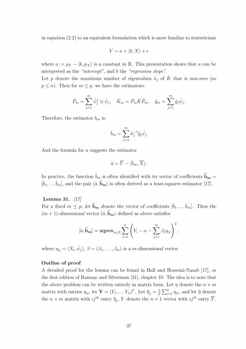
in equation (2.2) to an equivalent formulation which is more familiar to statisticians
Y = a+ 〈b,X〉+ ε
where a := µY − 〈b, µX〉 is a constant in R. This presentation shows that a can be
interpreted as the “intercept”, and b the “regression slope”.
Let p denote the maximum number of eigenvalues κj of K that is non-zero (so
p ≤ n). Then for m ≤ p, we have the estimators:
Pm =m∑j=1
ψ∗j ⊗ ψj, Km = PmKPm, gm =m∑j=1
gjψj.
Therefore, the estimator bm is:
bm =m∑j=1
κ−1j gjψj
And the formula for a suggests the estimator
a = Y − 〈bm, X〉.
In practice, the function bm is often identified with its vector of coefficients bm =
[b1, . . . bm], and the pair (a, bm) is often derived as a least-squares estimator [17].
Lemma 31. [17]
For a fixed m ≤ p, let bm denote the vector of coefficients [b1, . . . bm]. Then the
(m+ 1)-dimensional vector (a, bm) defined as above satisfies
[a, bm] = argmin[α,β]
n∑i=1
(Yi − α−
m∑j=1
βjηij
)2
,
where ηij = 〈Xi, ψj〉, β = (β1, . . . , βm) is a m-dimensional vector.
Outline of proof
A detailed proof for the lemma can be found in Hall and Hosseini-Nasab [17], or
the first edition of Ramsay and Silverman [31], chapter 10. The idea is to note that
the above problem can be written entirely in matrix form. Let η denote the n×m
matrix with entries ηij, let Y = (Y1, . . . Yn)T . Let ηj = 1
n
∑ni=1 ηij, and let η denote
the n×m matrix with ijth entry ηj, Y denote the n× 1 vector with ijth entry Y .
37
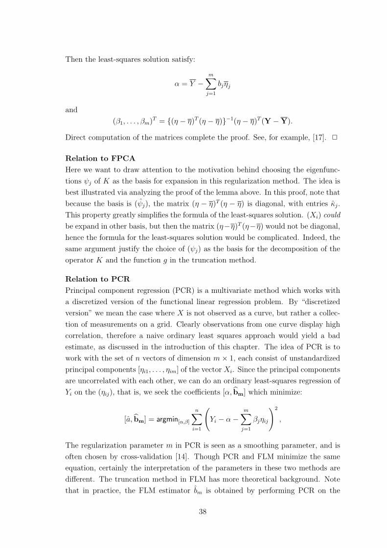
Then the least-squares solution satisfy:
α = Y −m∑j=1
bjηj
and
(β1, . . . , βm)T = (η − η)T (η − η)−1(η − η)T (Y −Y).
Direct computation of the matrices complete the proof. See, for example, [17]. 2
Relation to FPCA
Here we want to draw attention to the motivation behind choosing the eigenfunc-
tions ψj of K as the basis for expansion in this regularization method. The idea is
best illustrated via analyzing the proof of the lemma above. In this proof, note that
because the basis is (ψj), the matrix (η − η)T (η − η) is diagonal, with entries κj.
This property greatly simplifies the formula of the least-squares solution. (Xi) could
be expand in other basis, but then the matrix (η−η)T (η−η) would not be diagonal,
hence the formula for the least-squares solution would be complicated. Indeed, the
same argument justify the choice of (ψj) as the basis for the decomposition of the
operator K and the function g in the truncation method.
Relation to PCR
Principal component regression (PCR) is a multivariate method which works with
a discretized version of the functional linear regression problem. By “discretized
version” we mean the case where X is not observed as a curve, but rather a collec-
tion of measurements on a grid. Clearly observations from one curve display high
correlation, therefore a naive ordinary least squares approach would yield a bad
estimate, as discussed in the introduction of this chapter. The idea of PCR is to
work with the set of n vectors of dimension m× 1, each consist of unstandardized
principal components [ηi1, . . . , ηim] of the vector Xi. Since the principal components
are uncorrelated with each other, we can do an ordinary least-squares regression of
Yi on the (ηij), that is, we seek the coefficients [α, bm] which minimize:
[a, bm] = argmin[α,β]
n∑i=1
(Yi − α−
m∑j=1
βjηij
)2
,
The regularization parameter m in PCR is seen as a smoothing parameter, and is
often chosen by cross-validation [14]. Though PCR and FLM minimize the same
equation, certainly the interpretation of the parameters in these two methods are
different. The truncation method in FLM has more theoretical background. Note
that in practice, the FLM estimator bm is obtained by performing PCR on the
38
data first, then smooth the vector of coefficients using some interpolation method,
such as B-spline [8]. Therefore, we can view the idea behind PCR as an alternative
interpretation for lemma 31, that is, to regress Y on the firstm principal components
of X.
2.2.3 Choice of m and consistency
In this section, we study the effect of m on consistency properties of bm. We shall
see the crucial role that the accuracy-stability trade-off equation (2.7) plays in
determining the choice of m relative to n. Under certain conditions, convergence in
probability and almost surely of bm to b was established by Cardot et al. [7]. This
paper gives important bounds and results, though the English version contains
minimal discussions. Asymptotics and convergence in mean integrated squared
error are postponed to later sections, since they have interesting connections with
other problems.
As the diagram 2.6 suggested, we can view g as a perturbation of g, with distance
δ = ‖g − g‖ from the true function g. First, we need to obtain some bound on this
perturbation size in terms of n. Following chapter 1, we want to quantify the effect
of estimating X and Y separately. Therefore, define
g =1
n
n∑i=1
(Xi − µX)(Yi − µY ).
Then
‖g − g‖2 = ‖g − g‖2 + ‖g − g‖2 + 2‖g − g‖‖g − g‖.
Using the same proof idea as lemma 12 in chapter 1, we can show that ‖g − g‖ =
O(n−1). The following lemma gives a bound for ‖g − g‖:
Lemma 32. (Cardot et al.) [7]
If E ‖X‖4 <∞, then:
E ‖g − g‖2 ≤ ‖b‖2E ‖X − µX‖4
n+σ2
nE ‖X − µX‖2 .
Therefore,
E ‖g − g‖2 ≤ ‖b‖2E ‖X − µX‖4
n+σ2
nE ‖X − µX‖2 +O(n−2).
Proof: By definition of the L2-norm in L2(I), for any orthonormal basis (ej) of
39
L2(I), we have:
‖g‖2 =∞∑j=1
〈g, ej〉2.
Expand E‖g‖2, and use the independence of the (Xi), we obtain
E‖g‖2 =∞∑j=1
1
nE〈X − µX , ej〉(Y − µY )2 − 1
n‖g‖2 + ‖g‖2.
Write Y = µY + 〈b,X − µX〉+ ε, and use Cauchy-Schwarz inequality to get:
1
n
∞∑j=1
E〈X − µX , ej〉(Y − µY )2 ≤ 1
n
(‖b‖2E‖X − µX‖4 + σ2E‖X − µX‖2
).
And the bound for g follows. Coupled with the discussion before the lemma, we
obtain the bound for g. 2
Now write g as gn to emphasize its dependence on n. We can view (gn) as a sequence
of perturbations of g, with distance from the true function g being
δn := ‖gn − g‖ = O(n−1/2).
To bound ‖bm−bm‖, we cannot simply apply bound in equation (2.7), since we have
another source of perturbation comes from estimating K by K. One way to bound
this error is to write out the term (PmKPm)−1, then bounding the eigenfunction
estimators using proposition 16. This is done in [7], and the authors obtained the
following proposition
Proposition 33. (Cardot et al.) [7]
‖bm − bm‖ ≤ γn‖K − K‖∞ +1
κm‖g − gn‖+O(n−1)
where γn = 2‖g‖
1κmκm
+ 2( 1κm
+ 1κm
)∑m
j=1 aj
, with aj := 2
√2
ρj, where ρj was de-
fined in proposition 16.
The version stated above has an extra term O(n−1) compared to the version in
[7], which comes from estimating the mean. This does not affect the results at
order n−1/2, and in particular, the theorems on convergence almost surely and in
probability in [7] hold without modifications.
40
So the accuracy-stability trade-off equation for the sequence of estimators (bm) is
‖bm − b‖ ≤ O(κm+1) + γn‖K − K‖∞ +1
κm‖g − g‖+O(n−1).
For m = m(n) to be a regularization parameter on an event En, the right-hand
side needs to approach 0 as n→∞. Suppose, for a moment, that on an event En,
E(‖K − K‖∞|En
)= O(E‖K − K‖∞), E (‖g − gn‖|En) = O(E‖g − g‖), and that
C1km ≤ km ≤ C2km for some constants C1, C2 < ∞. Then using the bounds in
lemma 14 and proposition 32, E(‖bm − b‖|En
)can be bounded by
O(κ2m+1) +
O(n−1)
κ4m
+O(n−1)
κ2m
(∑mj=1 aj
)2 +O(n−1)
κ2m
.
This bound would converge to 0 if, for example, we had condition C1:limn→∞
nκ4m = ∞
limn→∞
nκ2m
(∑m
j=1 aj)2
= ∞.
Cardot et al. [7] considered the event
En = κm2< κm <
3κm2.
On En, γn ≤ υn = ‖g‖(
2κ2
m+ 6
κm
∑mj=1 aj
). Working with the tail probability rather
than the expectation directly, we obtain
P (‖b− bm‖ > η,En) ≤ P
(‖K − K‖∞ >
η
2υn
)+ P
(‖g − gn‖ >
κmη
4
).
To pass from tail probabilities to expectation, apply Chebychev’s inequality for the
right-hand side. Then we obtain an upper bound for P (‖b− bm‖ > η,En) in terms
of E‖K− K‖2 and E‖g− gn‖2. As discussed above, applying the bounds in lemma
14 and 32, we see that condition C1 is sufficient for this probability to converge to
0. A bound for P (En) comes from lemma 14, and hence under condition C1, this
quantity also converges to 0. This is the essence of the proof of the following result,
which was first stated in [7].
Theorem 34. (Cardot et al.) [7]
Let aj be defined as above. Let (m(n))n∈N∗ be a sequence of positive integers that
approaches ∞ as n→∞, with m(n) ≤ n. Assume the following:
41
• κ1 > κ2 > . . . > 0
• κ1 > κ2 > . . . > κm > 0
• E ‖X‖4 <∞.
• Condition C1:
limn→∞
nκ4m = ∞
limn→∞
nκ2m
(∑m
j=1 aj)2
= ∞.
Then:
‖bm − b‖ → 0 in probability as n→∞.
Comments: We note that the assumptions of the theorem are really basic: they
ensure that the estimator bm is well-defined and regularized. The first condition
eliminate any pathologies arising from aj blowing up because of ties in the eigen-
values sequence, the second condition ensures that each bj is well-defined, the third
condition allows the use of lemma 14 and 32, and the last condition ensures regu-
larity as discussed.
The bounds in lemma 14 and 32 are rather crude. Indeed, if we impose some
moment assumptions, almost sure convergence can be obtained for a slightly faster
convergence rate of the eigenvalues, while maintaining the regularization property.
Theorem 35. (Cardot) [7] Assume the following:
• κ1 > κ2 > . . . > 0
• κ1 > κ2 > . . . > κm > 0
• ‖X‖ ≤ c1 a.s. (That is, as a random variable mapping to L2(I), X is bounded
almost everywhere.)
• |ε| ≤ c2 a.s. (This means that the error is bounded almost everywhere)
• Condition C2:
limn→∞
nκ4m
log(n)= ∞
limn→∞
nκ2m
(∑m
j=1 aj)2 log(n)
= ∞.
Then:
‖bm − b‖ → 0 almost surely as n→∞
The proof of the above theorem can be found in [7]. We note that if the eigenvalues
κj decay geometrically or exponentially, an application of the theorems yield the
following corollary.
42
Corollary 36. If m(n) = o(log n), and κj = arj for some a > 0, r ∈ (0, 1) or
κj = aj−γ for some a > 0, γ > 1, then conditions (C1) and (C2) are satisfied.
Note the slow convegence rate of o(log n) on the sequence m for this case. If the
covariance function K is smooth (that is, the eigenvalues κj decay fast to 0), then
the regularity condition requires that m converges rather slowly. In practical terms,
a slowly increasing m implies that we need a very large increase in the sample size n
before we can add another term to the approximation bm. Intuitively this leads to a
poor convergence rate for bm. This rate can be improved if we work with a smooth
b, and if b is sufficient smooth relative to K, some optimal convergence rate can
be achieved. This is the idea behind the theorem by Hall and Horowitz [16] which
gives optimal mean integrated squared error converge rate of bm within a certain
class of estimators.
2.3 Mean integrated squared error
An important measure of the “goodness” of an estimator is the mean integrated
squared error (MISE) [23], which is defined as
MISE(bm) = E
∫I(bm − b)2 = E‖bm − b‖2.
We recognize that convergence in MISE is convergence in mean-square. Statistically,
a result on bounds or convergence MISE of bm is of great interest.
Under some smoothness and eigenvalue-decay assumptions, Hall and Hosseini-Nasab
[17] obtained: ∫IE(bm − b)2 ∼ σ2
n
m∑j=1
κ−1j +
∞∑j=m+1
b2j .
where σ2 = V ar(ε), and An ∼ Bn means that the ratio of the random variables
An and Bn converges to 1 as n → ∞. The eigenvalues κj here are assumed to be
decaying at a polynomial rate which favors a faster convergence of bm. The second
term on the right-hand side is the bias of the estimator bm, and the first term is
interpreted by the authors as the dominant term in the contribution of the error
bm − b to the integrated squared error. This term clearly shows the effect of the
decay rate of κj, but the lack of some type of O(nα) bound overall makes the result
difficult to interpret.
43
Hall and Horowitz [16] worked with exponentially decaying eigenvalues, but the
authors imposed a smoothness requirement on the function b to ensure that it is
sufficiently smooth relative to K. Their theorem states that under the assumptions
of the model, for some appropriate choices of m, bm achieves the optimal conver-
gence rate in MISE, which is a nonparametric rate. The authors also considered
an alternative regularization method, Tikhonov regularization, which is not based
on FPCA. It was shown that the same optimal rate is achieved under similar as-
sumptions. This implies that slow convergence rate is an intrinsic property of the
problem, rather than a property of the estimator.
We first introduce Tikhonov regularization for the purpose of comparing the optimal
MISE rate of its estimator with that obtained by truncation. Since this is the only
time we shall mention Tikhonov regularization in the thesis, only a brief summary
will be provided. Tikhonov regularization is an important method in solving inverse
problems. An introduction can be found in chapter 5 of Groetsch [15].
2.3.1 Tikhonov regularization
Here our notations and definitions follow that of Groetsch [15], chapter 5. Defini-
tions of the estimators follow that of Hall and Horowitz [16].
Consider the original ill-posed inverse problem
Kb = g.
In Tikhonov regularization, we want to approximate this with the equation
(K + λI)bλ = g, (2.8)
where λ > 0, I is the identity operator. Since K is a bounded positive semidefinite
operator, the operator (K + λI) is bounded and strictly positive, therefore it has a
bounded inverse. So provided that g ∈ R(K+λI)1, the inverse problem in equation
(2.8) is well-defined, and we have the solution
bλ = (K + λI)†g.
It can be shown that bλ → b as λ→ 0. Here λ is the regularization parameter (that
is, it plays the role of m). If δ denote a perturbation in g, then
‖bδλ − b‖ ≤ O(λ) + λ−1/2δ.
1which we can assume it to be, because N(K + λI) = 0 hence R(K + λI) is dense in L2(I)
44
This is the accuracy-stability trade-off equation for Tikhonov regularization, the
analogue of equation (2.7) in the truncation case.
In the FLM context, estimators in Tikhonov regularization are defined as follows:
the estimator for (K + λI)† is
K+ := (K + λI)−1.
This makes the estimator for bλ to be
bλ = K+g
where g and K are defined previously (in section 1).
It is important to note that the operator K+λI is not compact, therefore we do not
have the same kind of spectral representation as for K. In particular, the estimating
of b does not involve any basis expansion. Instead, the inverse (K+λI)† is computed
directly from the data, so we obtain a sequence of inverses (K†λ) := ((K + λI)†)
that converges to K† as λ→ 0. It is this property of Tikhonov regularization that
make the estimator robust to the eigenspacing problem.
2.3.2 MISE of the truncation method
Assume the following:
• Moment assumptions on X: X is assumed to have finite fourth-order moment,
in the sense that E‖X‖4 < ∞, E〈X,ψj〉4j < Cκ2j for all j, (where C > 1
denote a constant). The errors εi are independent and identically distributed,
zero mean, σ2 = V ar(εi) ≤ C.
• Decay rate of κj and bj: for some α > 1, β > 1 + 12α:
κj − κj+1 ≥ C−1j−α−1 for j ≥ 1, |bj| ≤ Cj−β.
Call these assumptions (A). Let F(C, α, β) denote the set of distributions of (X, Y )
that satisfy assumption (A), for given values of C, α, β. Let B denote the class of
measurable functions b of the data (X1, Y1), . . . , (Xn, Yn), generated by equation
(2.2). Then the theorem states that if we choose the truncation parameter m
correctly, that is, if m satisfies:2
m n1/(α+2β),
2where the relation rn sn for positive rn and sn means that the ratio between rn and sn isbounded away from zero and infinity.
45
then the resulting estimator bm is optimal in the class B, in the sense that it achieves
the fastest rate of convergence for the MISE in this context.
Theorem 37. (Hall and Horowitz) [16]
Assume the conditions (A) and that m n1/(α+2β). Then
limD→∞
lim supn→∞
supF∈F
PF
∫I(bm − b)2 > Dn−(2β−1)/(α+2β)
= 0 (2.9)
as n→∞. Further more, for any b ∈ B:
lim infn→∞
n(2β−1)/(α+2β) infb∈B
supF∈F
∫IEF (b− b)2 > 0.
The authors of the theorem noted that with some truncation of the term bm to
prevent it from taking too large values, the first equation of the theorem implies
that:
supF∈F
∫IEF (bm − b)2 = O(n−(2β−1)/(α+2β)), (2.10)
where b denote the truncated version of bm. This can be defined as follows [5]: for
some arbitrary chosen, fixed positive constant C3, C4, C5, let
bm =
bm, if ‖bm‖ ≤ C4n
C5
C3, otherwise(2.11)
Equation (2.10) shows that the MISE of bm converges to 0 at rate O(n−(2β−1)/(α+2β)).
The second equation in the theorem shows that any estimator b in B can only
obtain the rate O(n−(2β−1)/(α+2β)) at best. Therefore bm attains the optimal MISE
convergence rate in the class B.
Outline of proof
This is a rather technical proof, therefore we shall consider the main points only.
The idea is to quantify the errors from approximating ψj, κj and gj separately, give
bounds on these errors, and add up together to get a convergence rate for the MISE.
The authors defined bj = κ−1j gj, so bj− bj is the error from estimating gj by gj. This
error can be broken into three components: Sj1 = 〈g − g, ψj〉, which is the error
from estimating g by g, Sj2 = 〈g, ψj−ψj〉, which is the error from estimating ψj by
ψj, and Sj3 is the cross-term Sj3 = 〈g− g, ψj−ψj〉. Then under the assumptions of
the theorem, the authors obtained a bound for this term. Now, bj − bj is the error
46
comes from estimating κj by κj. Under assumptions of the theorem, and using
some bounds obtained from theorem 21, the authors showed that
m∑j=1
(bj − bj)2 = op(n
−(2β−1)/(α+2β)).
We have one more error, which is the bias term∑∞
j=m+1 b2j that comes from es-
timating b by bm. In [16], this is bounded by O(n−(2β−1)/(α+2β)). Therefore, the
Op(n−(2β−1)/(α+2β)) bound comes mainly from bounding the first term,∑m
j=1(bj − bj)2. So in some sense, the estimation of κj by κj does not influence the
convergence rate of bm as much as the estimation of gj by gj. Intuitively this should
be the case, as the later involves estimation of the eigenfunctions ψj.
Discussions
The moment assumption is not strict: a finite fourth-order moment is a basic re-
quirement to ensure consistency of the eigenvalues, eigenfunctions and the bm. The
good convergence rate is obtained not by smoothness of K, but by the relative
smoothness between bj and K. The condition β > 1 + 12α can be interpreted as b
being no less smooth than the lower bound of the smoothness of K, which is mea-
sured by the decay rate of its eigenvalues. As analyzed previously, this smoothness
assumption of b relative to K allows a good convergence rate for the estimator bm,
while keeping regularity.
It should be noted that the decay rate of κj is not written in the form κj ≥ Cj−α
for a constant C > 0, but rather in terms of eigenspacing. Indeed, this is not
equivalent: the spacing assumption implies κj ≥ Cj−α, but the reverse can fail, for
example, when there is a sequence of ties, or closedly spaced eigenvalues. A specific
example can found in [16]. This spacing requirement comes from the sensitivity of
the eigenfunction estimator ψj to eigenspacing, as analyzed in chapter 1. We shall
see in Tikhonov regularization that this eigenspacing assumption is not required,
because the method does not use ψj.
The tuning parameter m here is chosen to minimize the MISE, not merely to ensure
regularity. Of course some regularity is implicitly implied, as a larger-than-necessary
m leads to near-unstable behaviour of the equation Kmbm = gm, which results in a
large MISE. Note that with this m, under the assumptions of the model, condition
C2 in theorem 35 is satisfied. Indeed, m(n) increases much faster than the (albeit
conservative) rate o(log n) suggested in corollary 36. Again, this emphasizes the
importance of the relative smoothness assumption between b and K.
47
The optimal convergence rate under these conditions satisfies:
2β − 1
α+ 2β<
2β − 1
4β − 1<
1
2,
so estimating b is a nonparametric problem. The authors of the theorem noted that
this is a “typical” rate for ill-posed inverse problems [16]. This is demonstrated in
the following section, where we shall see that under similar conditions, Tikhonov
regularization also attains the same optimal rate.
2.3.3 MISE in Tikhonov regularization
In a similar context, Hall and Horowitz [16] in the same paper derived optimal MISE
convergence rate for the Tikhonov-regularized estimator b. The moment assumption
is the same, however, the decay rate is replaced by the following conditions:
For some α > 1, β > α− 12:
Cκj ≥ j−α for j ≥ 1, |bj| ≤ Cj−β.
Denote this and the moment condition by assumption (B). Let G(C, α, β) denote
the set of distributions F of (X, Y ) that satisfy assumption (B). Then we have the
following theorem.
Theorem 38. (Hall and Horowitz) [16]
If assumption (B) holds, and if the tuning parameter λ satisfies
λ n−α/(α+2β), (2.12)
then
supF∈G
∫IEF (b− b)2 = O(n−(2β−1)/(α+2β))
as n→∞. Furthermore,
lim infn→∞
n(2β−1)/(α+2β) infb∈B
supF∈G
∫IEF (b− b)2 > 0.
The two bounds have similar interpretations to those in theorem 37. The first equa-
tion shows the performance of b, and the second equation shows the performance
of any estimator b in the class B. Together, the two equations imply that b obtain
the optimal MISE convergence rate, which is O(n−(2β−1)/(α+2β)).
48
Discussions
The slight difference in the relation between β and α between the two theorems
is unimportant. If β > max(α − 12, 1
2α + 1), then the two theorems give the same
optimal MISE convergence rates. Note that the decay condition in Tikhonov reg-
ularization is of the form Cκj ≥ j−α rather than in terms of eigenspacing, which
implies that the method is robust against closedly spaced or equal eigenvalues.
This is consequence of not having to estimate the eigenfunctions ψj in Tikhonov
regularization.
2.4 Selected topics in FLM
2.4.1 Prediction
In practice, estimation of b is arguably not as important as the esitmation of Y
given X = x. This is termed the “prediction problem”. Specifically, given that X
and Y satisfies the functional linear model, we want to find
E(Y |X = x) = a+ 〈b, x〉. (2.13)
The theoretical aspects of the prediction problem were discussed in Cai and Hall
[5], where a mean-squared convergence rate was derived. This paper considered
the case of estimating b by truncation, and quantified the effect of the relative
smoothness between x, b and K on the convergence rate. Cardot et al. [10] derived
a central limit theorem for the estimator b as well as the predictor 〈b, x〉 for a range
of regularized estimators for b, including those obtain by truncation and Tikhonov
regularization. This paper underlined the difference between the two problems:
it was shown that no central limit theorem exists for b, while some asymptotic
normality holds for 〈b, x〉. Other work on the prediction problem include that of
Cuevas et al. [11], where the case of Y ∈ L2(I) was considered, Ferraty and Vieu
[13], where nonparametric approaches to the functional prediction problem were
discussed in details. Here we shall only analyze two papers of Cai and Hall [5] and
Cardot et al. [10], since they utilize the truncation estimator.
Consider the method of regularization by truncation. An estimate for equation
(2.13) would be
a+ 〈bm, x〉 = a+
∫Ibmx = a+
m∑j=1
bjxj,
where xj := 〈x, ψj〉, and a is
a = Y − 〈bm, x〉.
49
As noted in [5], the operation of integration gives additional smoothness, therefore
an optimal choice of 〈bm, x〉 to minimize the mean-squared error would involve
an undersmoothed bm (relative to the optimal choice of bm in theorem 37). This
implies a possibly better convergence rate for 〈bm, x〉, and hence sets the prediction
problem apart from the problem of estimating b. Indeed, this distinction can be
seen by comparing theorem [16] with the theorem in Cai and Hall [5]. We shall
state the later theorem below.
Assume the following:
• Eigenvalues decay rate and spacing: C−1j−α ≤ κj ≤ Cj−α, and κj − κj+1 ≥C−1j−α−1 for j ≥ 1.
• Moment assumption: all the moments of X are finite. Specifically, for each
r ≥ 2 and each j ≥ 1, E‖ξj‖2r < C(r)κrj , where ξj is the unstandardized
principal component of X, C(r) does not depend on j, and for any sequence
j1, . . . j4, E(ξj1ξj2ξj3ξj4) = 0 unless each index jk is repeated. All moments of
the distribution of the errors εi are finite.
• Smoothness of b: |bj| ≤ C1j−β for each j ≥ 1.
• Smoothness of x: |xj| ≤ C2j−γ for each j ≥ 1.
• Relative smoothness between x, b and K: α > 1, β ≥ α+ 2, and γ > 12.
Collectively, call the conditions above assumption (A). Define B(C1, β) to be the set
of b =∑∞
j=1 bjψj such that bj satisfies the smoothness condition above for chosen
C1, β. Like in theorem 37, let bm denote the truncated version of bm (recall equation
(2.11)). The convergence rate of 〈bm, x〉 to 〈b, x〉 depends on the relation between
α and γ.
Theorem 39. (Cai and Hall) [5]
Under assumption (A), suppose that the truncation parameter m is chosen as fol-
lows: m m0, where
m0 =
n1/2(β+γ−1), if α+ 1 < 2γ,
(n/ log n)1/(α+2β−1), if α+ 1 = 2γ,
n1/(α+2β−1), if α+ 1 > 2γ.
Then, for each given C,C1, . . . , C5 > 0, as n → ∞, the estimator bm defined in
equation (2.11) satisfies
supb∈B(C1,β)
E(〈bm, x〉 − 〈b, x〉
)2
= O(τ)
50
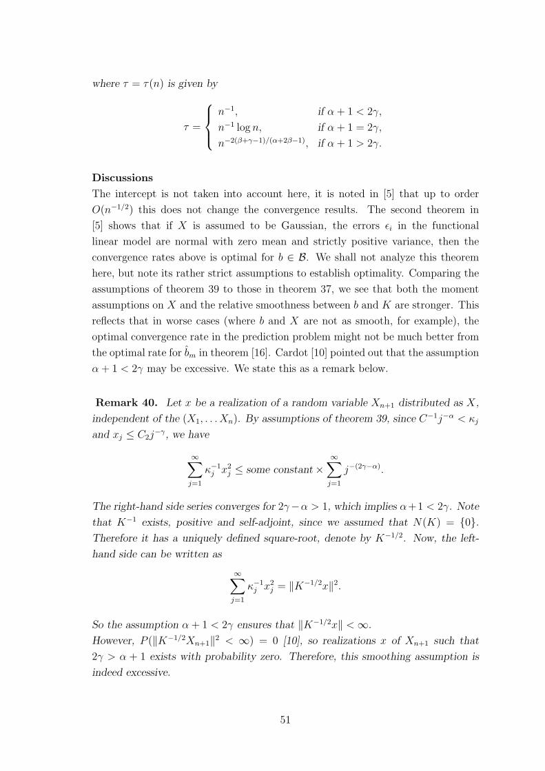
where τ = τ(n) is given by
τ =
n−1, if α+ 1 < 2γ,
n−1 log n, if α+ 1 = 2γ,
n−2(β+γ−1)/(α+2β−1), if α+ 1 > 2γ.
Discussions
The intercept is not taken into account here, it is noted in [5] that up to order
O(n−1/2) this does not change the convergence results. The second theorem in
[5] shows that if X is assumed to be Gaussian, the errors εi in the functional
linear model are normal with zero mean and strictly positive variance, then the
convergence rates above is optimal for b ∈ B. We shall not analyze this theorem
here, but note its rather strict assumptions to establish optimality. Comparing the
assumptions of theorem 39 to those in theorem 37, we see that both the moment
assumptions on X and the relative smoothness between b and K are stronger. This
reflects that in worse cases (where b and X are not as smooth, for example), the
optimal convergence rate in the prediction problem might not be much better from
the optimal rate for bm in theorem [16]. Cardot [10] pointed out that the assumption
α+ 1 < 2γ may be excessive. We state this as a remark below.
Remark 40. Let x be a realization of a random variable Xn+1 distributed as X,
independent of the (X1, . . . Xn). By assumptions of theorem 39, since C−1j−α < κj
and xj ≤ C2j−γ, we have
∞∑j=1
κ−1j x2
j ≤ some constant×∞∑j=1
j−(2γ−α).
The right-hand side series converges for 2γ−α > 1, which implies α+1 < 2γ. Note
that K−1 exists, positive and self-adjoint, since we assumed that N(K) = 0.Therefore it has a uniquely defined square-root, denote by K−1/2. Now, the left-
hand side can be written as
∞∑j=1
κ−1j x2
j = ‖K−1/2x‖2.
So the assumption α+ 1 < 2γ ensures that ‖K−1/2x‖ <∞.
However, P (‖K−1/2Xn+1‖2 < ∞) = 0 [10], so realizations x of Xn+1 such that
2γ > α + 1 exists with probability zero. Therefore, this smoothing assumption is
indeed excessive.
51
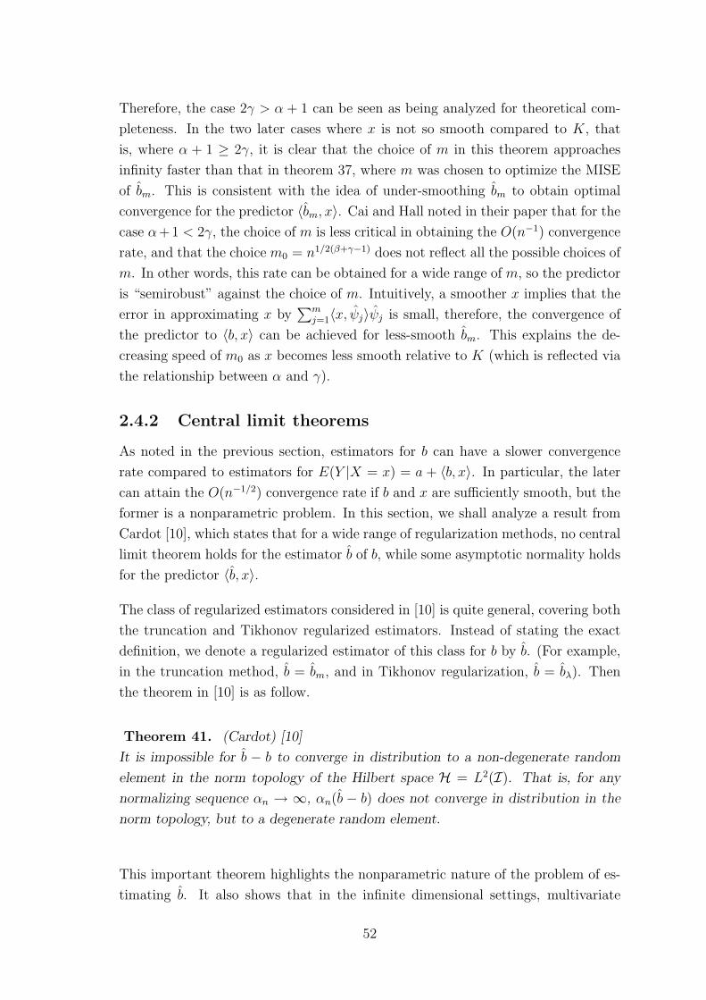
Therefore, the case 2γ > α + 1 can be seen as being analyzed for theoretical com-
pleteness. In the two later cases where x is not so smooth compared to K, that
is, where α + 1 ≥ 2γ, it is clear that the choice of m in this theorem approaches
infinity faster than that in theorem 37, where m was chosen to optimize the MISE
of bm. This is consistent with the idea of under-smoothing bm to obtain optimal
convergence for the predictor 〈bm, x〉. Cai and Hall noted in their paper that for the
case α+1 < 2γ, the choice of m is less critical in obtaining the O(n−1) convergence
rate, and that the choice m0 = n1/2(β+γ−1) does not reflect all the possible choices of
m. In other words, this rate can be obtained for a wide range of m, so the predictor
is “semirobust” against the choice of m. Intuitively, a smoother x implies that the
error in approximating x by∑m
j=1〈x, ψj〉ψj is small, therefore, the convergence of
the predictor to 〈b, x〉 can be achieved for less-smooth bm. This explains the de-
creasing speed of m0 as x becomes less smooth relative to K (which is reflected via
the relationship between α and γ).
2.4.2 Central limit theorems
As noted in the previous section, estimators for b can have a slower convergence
rate compared to estimators for E(Y |X = x) = a + 〈b, x〉. In particular, the later
can attain the O(n−1/2) convergence rate if b and x are sufficiently smooth, but the
former is a nonparametric problem. In this section, we shall analyze a result from
Cardot [10], which states that for a wide range of regularization methods, no central
limit theorem holds for the estimator b of b, while some asymptotic normality holds
for the predictor 〈b, x〉.
The class of regularized estimators considered in [10] is quite general, covering both
the truncation and Tikhonov regularized estimators. Instead of stating the exact
definition, we denote a regularized estimator of this class for b by b. (For example,
in the truncation method, b = bm, and in Tikhonov regularization, b = bλ). Then
the theorem in [10] is as follow.
Theorem 41. (Cardot) [10]
It is impossible for b − b to converge in distribution to a non-degenerate random
element in the norm topology of the Hilbert space H = L2(I). That is, for any
normalizing sequence αn → ∞, αn(b − b) does not converge in distribution in the
norm topology, but to a degenerate random element.
This important theorem highlights the nonparametric nature of the problem of es-
timating b. It also shows that in the infinite dimensional settings, multivariate
52
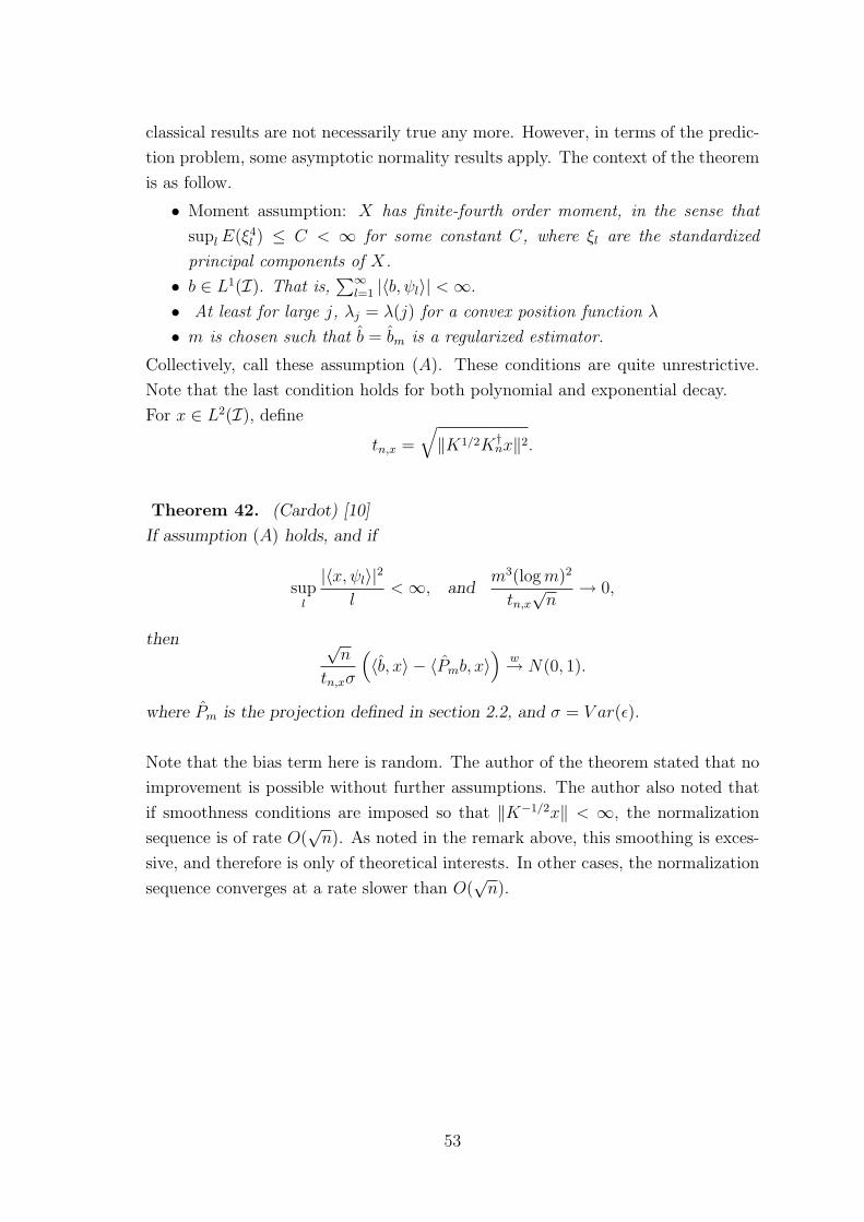
classical results are not necessarily true any more. However, in terms of the predic-
tion problem, some asymptotic normality results apply. The context of the theorem
is as follow.
• Moment assumption: X has finite-fourth order moment, in the sense that
suplE(ξ4l ) ≤ C < ∞ for some constant C, where ξl are the standardized
principal components of X.
• b ∈ L1(I). That is,∑∞
l=1 |〈b, ψl〉| <∞.
• At least for large j, λj = λ(j) for a convex position function λ
• m is chosen such that b = bm is a regularized estimator.
Collectively, call these assumption (A). These conditions are quite unrestrictive.
Note that the last condition holds for both polynomial and exponential decay.
For x ∈ L2(I), define
tn,x =
√‖K1/2K†
nx‖2.
Theorem 42. (Cardot) [10]
If assumption (A) holds, and if
supl
|〈x, ψl〉|2
l<∞, and
m3(logm)2
tn,x√n
→ 0,
then √n
tn,xσ
(〈b, x〉 − 〈Pmb, x〉
)w→ N(0, 1).
where Pm is the projection defined in section 2.2, and σ = V ar(ε).
Note that the bias term here is random. The author of the theorem stated that no
improvement is possible without further assumptions. The author also noted that
if smoothness conditions are imposed so that ‖K−1/2x‖ < ∞, the normalization
sequence is of rate O(√n). As noted in the remark above, this smoothing is exces-
sive, and therefore is only of theoretical interests. In other cases, the normalization
sequence converges at a rate slower than O(√n).
53
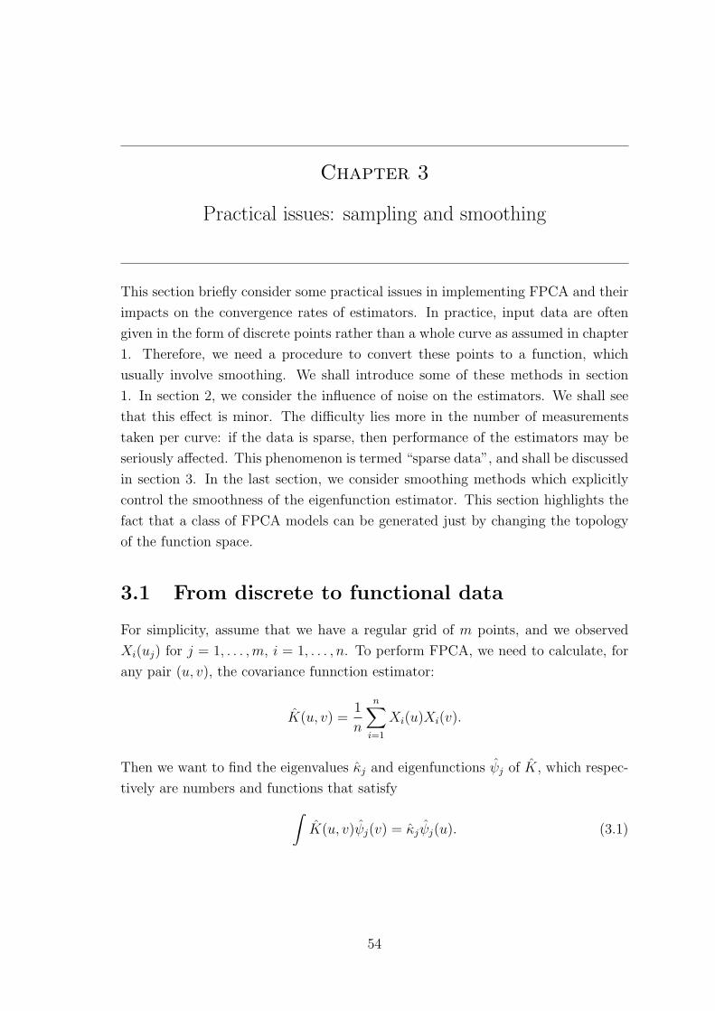
Chapter 3
Practical issues: sampling and smoothing
This section briefly consider some practical issues in implementing FPCA and their
impacts on the convergence rates of estimators. In practice, input data are often
given in the form of discrete points rather than a whole curve as assumed in chapter
1. Therefore, we need a procedure to convert these points to a function, which
usually involve smoothing. We shall introduce some of these methods in section
1. In section 2, we consider the influence of noise on the estimators. We shall see
that this effect is minor. The difficulty lies more in the number of measurements
taken per curve: if the data is sparse, then performance of the estimators may be
seriously affected. This phenomenon is termed “sparse data”, and shall be discussed
in section 3. In the last section, we consider smoothing methods which explicitly
control the smoothness of the eigenfunction estimator. This section highlights the
fact that a class of FPCA models can be generated just by changing the topology
of the function space.
3.1 From discrete to functional data
For simplicity, assume that we have a regular grid of m points, and we observed
Xi(uj) for j = 1, . . . ,m, i = 1, . . . , n. To perform FPCA, we need to calculate, for
any pair (u, v), the covariance funnction estimator:
K(u, v) =1
n
n∑i=1
Xi(u)Xi(v).
Then we want to find the eigenvalues κj and eigenfunctions ψj of K, which respec-
tively are numbers and functions that satisfy∫K(u, v)ψj(v) = κjψj(u). (3.1)
54
To obtain these estimators based on the measurements observed at the m points
u1, . . . um, there are, in general, two approaches: “interpolation” and “basis expan-
sion”. A survey of both techniques can be found in Ramsay and Silverman [31],
therefore, only a brief account shall be provided here.
Method 1: interpolation from multivariate PCA
This is the earliest approach to FPCA, used independently by Rao and Tucker, both
in 1958, who applied multivariate PCA without modification to observed function
values [31]. Under the multavirate PCA viewpoint, the covariance matrix is an
m×m matrix, with jkth entry:
K(uj, uk) =1
n
n∑i=1
Xi(uj)Xi(uk).
Standard multivariate techniques yield the eigenvectors ψj, and the eigenvalues κj
of K. Then the function ψj is obtained from ψj via interpolation (more accurately,
by applying a standard smoothing technique such as kernel smoothing). The final
formula contains a weight correction term which comes from the choice of numer-
ical integration technique to evaluate (3.1). Details can be found in Ramsay and
Silverman [31].
Clearly when using this method, we are essentially smoothing the principle fac-
tors obtained from multivariate PCA. With this approach, in practical terms, the
multivariate and the functional viewpoints do not differ significantly. The func-
tional approach has the advantage of providing a viewpoint which has substantial
theoretical background, therefore allow further developments. Indeed, as noted in
chapter 2, though the estimator obtained from the truncation approach to FLM can
be viewed as the result of interpolating the vector obtained from PCR. However,
the theoretical background of FLM pointed out that the problem is intrinsically
nonparametric, while this can be difficult to infer from the PCR viewpoint.
Method 2: basis function expansion
Suppose that we choose some basis (φl) of L2(I) to approximate X by the p-term
sum:
X ≈ X =
p∑l=1
〈X,φl〉φl =
p∑l=1
clφl = CΦ.
Clearly X lies in a p-dimensional subspace of L2(I), hence its covariance function
K can only have at most p non-zero eigenfunctions. Let Ψ denote the p× 1 matrix
55
of eigenfunctions of K. Then K and Ψ can be written in matrix terms
K(u, v) = EΦT (u)CTCΦ(v), Ψ = BΦ, ψj = bjΦ = ΦT bTj ,
where bj denote the jth row of B, B defined by Ψ = BΦ. By identifying Ψ with B,
X with C, we see that estimating the eigenfunctions is a p-dimensional problem of
finding the p× p matrix B. Equation (3.1) now reads∫K(u, v)ψj(v) = E
∫ΦT (u)CTCΦ(v)ΦT (v)bTj dv
= EΦT (u)CTCWbTj = κjΦT (u)bTj ,
where W =∫
Φ(v)ΦT (v) dv. This implies the purely matrix equation:
E(CTCWbTj ) = κjbTj .
Since Φ is known,W is known, and C can be approximated by numerical integration,
we can solve the above equation to obtain B, and hence find the eigenfunctions Ψ.
The basis expansion method is convenient for computation, since it reduces the
problem directly to a matrix formula. Clearly the choice of basis (φl) is the crucial
step here. In practice, (φl) is chosen based on data features [31].
Both methods extend naturally to the case of FLM. As mentioned in chapter 2,
the interpolation method in the FLM context corresponds to performing PCR on
the discretized data. Implicit smoothing is done in both approaches. In the in-
terpolation method, numerical integration of equation (3.1) and the interpolation
(or rather, smoothing) step gives a smooth estimate for ψj. In the basis expansion
method, numerical integration of C, and the choice of p correspond to a smoothing
of the input data X, and hence result in smooth estimates of the eigenfunctions
(ψj). Accuracy of the approximation depends on these steps. If the measurements
are observed on a dense grid and if X is smooth, a situation which usually arises
when the data are recorded by some automated instrument, then the numerical ap-
proximation performs quite well, and the choice of numerical method usually does
not have a great effect. However, if the data are sparse, estimators obtained this
way can be highly biased. Hence a different treatment is required. We shall discuss
this in section 3.
56
3.2 A model for noise
Suppose we are given a set Y = Y1, . . . , Yn of independent random functions,
identically distributed as Y , with:
Y (t) = X(t) + ε(t),
where X is a stochastic process defined on a compact set I, with finite mean-
trajectory:∫I E(X2) < ∞, and the set of random variables ε(t) : t ∈ I are
independent, identitcally distributed as ε, with Eε = 0, V arε = σ2 < ∞. Sup-
pose that X and ε are independent. ε represents the noise, X represents the true
underlying process. We are interested in estimating the true eigenfunctions and
eigenvalues of X from the observations (Yi).
In the basis expansion method, a maximum likelihood approach is often employed
to estimate the matrix B. Therefore the noise is often assumed to be Gaussian,
and it does not significantly affect the estimates [29]. In the interpolation method,
note that E[Y (u)Y (v)] = E[X(u)X(v)] + σ2δuv where δuv is the Kronecker’s delta
function. So the error really only have an effect on the trace of the covariance
function. In practice, for example, see [36], this is dealt with by ignoring the trace
of the covariance function KY in calculations. Then, the covariance matrix would
be a (m− 1)× (m− 1) matrix, with entries:
K(uj, uk) =1
n
n∑i=1
Xi(uj)Xi(uk), j 6= k
This results in eigenfunction estimators ψj being vectors of m − 1 dimension, and
from there, the interpolation method is applied as usual.
We state our conclusion as a remark below.
Remark 43. In both interpolation and basis expansion methods, identically
distribued, independent noise with constant variance does not make a significant
difference in calculating the eigenfunctions and eigenvalues.
3.3 Sparsity
Accuracy of the numerical methods mentioned in section 1 depends on the resolving
power of data, that is, the number of measurements made per curve, m, relative to
the amount of curvature in the data [31]. For example, if the underlying curveX has
57
many high-frequency terms, then we need more measurements per curve to achieve
the same magnitude in error, as compared to the case where X is a very flat curve
(has more low-frequency terms). Here we consider the case where the underlying
curve X is smooth, but m is small. This situation is called “sparse data”, a setting
typically seen in longitudinal studies. Direct application of either methods in section
1 would lead to bad estimates due to the high bias from evaluating the integrals
numerically. However, either methods can be adapted to this setting.
Under the basis expansion framework, if X a Gaussian process, the usual approach
in literature involves finding B using maximum likelihood. James et al. [21] con-
sidered an EM algorithm method, while Peng and Paul [29] noticed that B lies in
a Stiefel manifold1, which is a Riemann surface and hence have nicely defined tan-
gents. Therefore, the authors proposed a Newton-Raphson algorithm to maximize
the likelihood. Other papers under the basis expansion framework can be found in
Peng and Paul [29] and references therein. For the interpolation approach, kernel
smoothing is often employed to obtain a smooth estimate of the observed covariance
function, then the eigenfunctions and eigenvalues are estimated as usual [36]. Hall
et al. [20] used a local linear smoother and proved optimality of this procedure
under rather weak assumptions on the process for optimal choice of bandwidths.
We shall not analyze these results in details here. It is worth summarizing thereom
1 in [20], however, since this would give us some intuition on the effects of sparsity
on convergence rates.
Remark 44. Theorem 1 in [20] can be summarized as follows. Assume that we
observe mi random measurements on the ith curve, mi fixed. Under some weak
smoothness conditions on X, if the smoothing bandwidth is chosen correctly, then
the resulting eigenvalue estimator κj is still root-n consistent, but the eigenfunction
estimator converges at a much slower rate:
‖ψj − ψj‖ = Op(n−2/5).
It should be noted that if the mi measurements were fixed points, then convergence
would not take place: there are infinitely many curves in L2(I) that can produce the
same observed values. Therefore, the randomness of the sampling scheme ensured
convergence as n→∞. However, Hall et al. [20] showed that if the data collected
on a fixed or random grid is allowed to be increasingly dense, that is, m → ∞ as
1Stiefel manifold: the space of real valued matrices with orthonormal columns
58
n → ∞ at a rate faster than O(n−1/4), then the estimators produced are root-n
consistent to the estimators that we would construct if theXi were directly observed.
That is,
‖ψj − ψj‖ = Op(n−1/2),
where ψj is the estimator produced under the sparse model, and ψj is the estimator
produced when we observe the full curves (Xi).
As mentioned, sparse data is a situation typically seen in longitudinal studies, a
field where much development has been in the parametric direction. It is only in
the past few years that the parallel between functional sparse data and longitudinal
data were drawn [32, 20, 36, 29]. Much research in this direction is still being done.
3.4 Smoothing with a roughness penalty
The aim of smoothing in FPCA is to obtain smooth estimators of the eigenfunc-
tions (ψj). This can be achieved by smoothing the input data Xi, smoothing the
covariance function K, or smoothing the eigenfunctions (ψj). From this viewpoint,
it is clear that some smoothing is already imposed by the conversion of the dis-
crete measurements to a functional observation, especially in the sparse data case.
However, even when the whole curve is observed, smooth estimators may be desir-
able. Several procedures have been proposed: kernel smoothing of the covariance
function [3], ridge regression [30], change of inner product [33]. In this section, we
shall consider the last two methods and their relationships. In particular, we shall
demonstrate the idea that by changing in the geometry of the function space, we
can obtain a range of eigenfunction estimators from the same data.
3.4.1 Ridge regression
One of the first papers on ridge regression in FPCA was written by Ramsay and
Silverman [30]. The idea is to view FPCA as a problem of minimizing the expected
mean squared error, and attach a roughness penalty to this equation to obtain
smoother estimates of the eigenfunctions ψj. Ramsay and Silverman [31] suggested
to take ‖D2ψj‖2 as the roughness penalty, where D denote the differential operator.
Let V denote the subspace of L2(I) where φ ∈ V ⇒ D2φ ∈ L2(I). Then, the
procedure is to find a set of orthonormal basis (φi)Mi=1 of L2(I) that minimize
E
∥∥∥∥∥X −M∑i=1
〈X,φi〉φi
∥∥∥∥∥2
+ λ‖D2φi‖2, (3.2)
59
where λ > 0 is a smoothness parameter. As λ → ∞, we obtain very smooth
estimates since more penalty are put on the norm of the second derivative of φi.
Similarly, the estimates become rougher as λ → 0. The first edition of the book
by Ramsay and Silverman [31] contains details on implementing this method in
practice. Though the idea of ridge regression is familiar to statisticians, it is difficult
to integrate this method into a linear operator framework. It is also not clear if this
is equivalent to first smooth the data, then perform FPCA. Indeed, there is a close
connection between smoothing the input data X and smoothing the eigenfunctions
ψj, and this link has been established in many different settings, for example, [31,
33, 28, 3]. Therefore, we shall consider another roughness penalty method.
3.4.2 A change in norm
Silverman [33] suggested to attach a roughness penalty into the definition of the
inner product iself. The author suggested to consider functions from a subset of
the Sobolev space W (2,2):
V =f ∈ W (2,2), D4f ∈ L2(I), D2f = D3f = 0 at the boundary of I
,
and provide this space with an inner product which is a slight generalization of the
usual W (2,2) inner product, defined by:
〈·, ·〉α : V × V → R, 〈f, g〉α = 〈f, g〉+ α〈D2f,D2g〉,
where 〈·, ·〉 denote the usual L2-norm, D is the differential operator, and α is a
chosen, fixed number, α ≥ 0. Then we perform FPCA on V . In other words, we
want to find M eigenfunction estimators (ψi)Mi=1, orthornomal in V , such that they
are the solution to
argmin(φi):〈φi,φj〉α=δij
E
∥∥∥∥∥X −M∑i=1
〈X,φi〉α φi
∥∥∥∥∥2
α
. (3.3)
To see how this is related to smoothness, the key step is to establish a relationship
between performing FPCA with respect to the proposed inner product and perform-
ing a certain FPCA with respect to the L2 inner product. Consider the space and
the inner product defined. The conditions on V ensure thatD2 is a self-adjoint linear
operator. Then, since D4 maps V to L2(I), we can write: 〈D2f,D2g〉 = 〈D4f, g〉.So:
〈f, g〉α = 〈Tf, g〉
60
where T = I + αD4 is an operator (I is the identity operator). Further, since T is
a self-adjoint, strictly positive linear operator, it has a unique self-adjoint, strictly
positive square-root, denoted by S. (See, for example, Wouk [35]). Note that S−1
is also self-adjoint. Then:
〈f, g〉α = 〈Sf, Sg〉.
Now, consider the effect of performing FPCA in V . Recall that the FPCA eigenbasis
in L2(I) can be derived as the orthonormal sequence which at the ith step maximizes:
E〈X,φi〉2,
subject to ‖φi‖ = 1, and that φi is orthogonal to all other φj with j < i. With the
new inner product, we want to maximize:
E〈X,φi〉2 = E(〈S S−1X,φi〉)2 = E(〈S−1X,Sφi〉)2,
under the orthonormal constraint: 〈φi, φj〉α = 〈Sφi, Sφj〉 = δij. We recognize
this as equivalent to performing PCA on the transformed data Y = S−1X, which
yields eigenfunction estimators (Sψi), and from there (ψi) can be recovered by
applying S−1. Silverman [33] interpreted S−1 as a smoothing operator. So the
FPCA performed in this new space can be interpreted as PCA of smoothed data.
It can be proved quite easily that this approach maximizes [33]
E(〈X,φi〉)〈φi, φi〉+ α〈D2φi, D2φi〉
.
In the ridge regression method, minimizing equation (3.2) under the orthonormal
constraint for the (φi) is equivalent to maxmizing:
E(〈X,φi〉)− α〈D2φi, D2φi〉
〈φi, φi〉. (3.4)
We note that the change-in-norm approach is closely related to ridge regression.
This method also has a clear geometrical interpretation and is easy to implement in
practice [33]. Ocana et al. [28] and Ferraty and Vieu [13] generalized this approach
into a systematic way of obtaining new FPCA estimators from the same data by
changing the topology of the space. This is an active research topic in FDA.
61
Chapter 4
Concluding Remarks
4.1 A summary of the thesis
The idea of FPCA is to retain the first m terms of the Karhunen-Loeve expansion
as an approximation to the data. Provided that the eigenvalues decay to zero fast
enough, the functional data problem is converted to an m-dimension multivariate
problem. If we observe the whole curve Xi for each i, estimating the eigenvalues
and eigenfunctions in FPCA are shown to be semiparametric problems: the esti-
mators attain the optimal root-n convergence rate. The key property that set func-
tional data apart from other multivariate high dimensional problems is that there
is no“curse of dimensionality” present, due to the covariance function being fixed
rather than increasing with the sample size. Theoretically, closely spaced eigenval-
ues is a concern, as they slow down on the convergence rate of the corresponding
eigenfunctions.
In practice, closedly spaced eigenvalues are rare. A more important issue of concern
is the sampling rate: since we often only observe points on Xi rather than the whole
curve, the number of sampled points affect convergence rates. In particular, the
sparser the sampling points, the worse the estimators become. If the measurements
are made at fixed points on the interval, clearly no convergence can be achieved.
However, if the measurements are sampled randomly rather than at fixed intervals,
the estimators for the eigenvalues can be shown to converge at the parametric rate
O(n−1/2), while those for the eigenfunctions converge at a slower rate O(n−2/5)
(using a smoothed estimate for the covariance function with an appropriate choice
of bandwidth). The sparse data problem is one distinct feature of functional data,
and it highlights one of the differences between functional and multivariate settings.
FLM is an important area of FDA where FPCA methods can be effectively applied.
Unlike the finite-dimensional case, the problem of estimating the regression slope
an ill-posed inverse problem, therefore, the estimator converges at a nonparametric
rate. The convergence rate is better for the prediction problem, and under very
62
strict smoothness assumptions, the predictor achieves the parametric rate. No cen-
tral limit theorem exists for a wide class of estimators for the regresion slope. These
problems do not exist in the finite-dimensional case, since the corresponding inverse
problem is well-posed. This is another important difference between functional and
multivariate settings which was explored in this thesis.
4.2 Further topics
Multivariate FPCA
In this thesis we only worked with the Hilbert space L2(I), where I is assumed
to be a compact subset of R. It is not difficult to extend the theory of FPCA to
the case where X is a random function of several variables. In fact, the setting
considered by Dauxois et al. [12] was more general, with I = (I, µ) abstractly
defined as a measurable space with bounded measure µ. Hence, consistency and
asymptotic results extend readily to this case with little changes. In practice, this
extension is potentially useful in analyzing spatial data, for example. Another way
to obtain a “multivariate-functional” setting is to consider the case where X is a
vector of random functions. One can take direct sum of Hilbert spaces to reduce the
problem to the “univariate-functional” situation considered. For example, Ramsay
and Silverman [31] in chapter 10 considered the case of “mixed data” where X1 is
a random function in L2(I), and X2 is a random vector. Then in this case, we can
work with random functions X which take values in H = L2(I) ⊕ Rd. Again, the
theory changes very little when we extend to these cases, although the practical
details might be slightly different [31].
New models by changing the topology
As mentioned in the last section of chapter 3, certain methods of smoothing by
roughness penalty can be incorporated into a linear operator framework. Ocana et
al. [28] considered a large class of inner products and generalized this approach.
The authors obtained a relationship between performing FPCA with respect to a
different inner product, and performing FPCA on transformed data in the usual L2
inner product. Their paper highlights the fact that a class of inner products can
give rise to a class of FPCA models for the same data. As a further generalization,
Ferraty and Vieu [13] worked with semi-norm, and also noted that many new models
can be constructed just by changing the topological structure of the space we work
with. Model selection would be of interest in this situation, and this is another
active research area in functional data analysis. [13]
63
Hypothesis testing
The statistical inference component of FPCA is still under research. Ferraty and
Vieu [13] pointed out that hypothesis testing is an important area of functional
data analysis. Some work in this direction include that of Hall and Vial [19], on
testing the infinite dimensionality of the data, Cardot et al. [9], on testing of no-
linear-relationship between Y and X in FLM.
An alternative to FPCA: nonparametric methods
Apart from FPCA, there are other alternative tools in analyzing FDA, some of
which are outlined in the book by Ramsay and Silverman [31]. An active area of
research is that of nonparametric methods, where kernel methods are extended to
the functional setting. Ferraty and Vieu [13] contains an overview of both practical
and theoretical aspects of this approach. The book also contains a list of open
research problems, some of which have been (partly) answered in the recent years.
Some papers in this direction include those of Mas [26], Berlinet et al. [1], Cardot
et al. [6]. This is an active research area in functional data analysis.
64
References
[1] Berlinet, A., Elamine, A. and Mas, A. Local linear regression for functional
data, In print.
[2] Besse, P. PCA stability and choice of dimensionality. Statistics and Probability
Letters, 13:405–410, 1992.
[3] Boente, G. and Fraiman, R. Kernel-based functional principal components.
Statistics and Probability letters, 48:335–345, 2000.
[4] Bosq, D. Linear processes in function spaces. Springer, 2000.
[5] Cai, T. T. and Hall, P. Prediction in functional linear regression. The Annals
of Statistics, 34:2159–2179, 2006.
[6] Cardot, H. Nonparametric regression for functional responses with application
to conditional functional principal components analysis, Technical report 2005,
Universite Paul Sabatier.
[7] Cardot, H., Ferraty, F. and Sarda, P. Functional linear model. Statistics and
Probability Letters, 45:11–22, 1999.
[8] Cardot, H., Ferraty, F. and Sarda, P. Spline estimators for the functional linear
model. Statistica Sinica, 13:571–591, 2003.
[9] Cardot, H., Goia, A. and Sarda, P. Testing for no effect in functional lin-
ear regression models, some computational approaches. Communications in
statistics, 33:179–199, 2004.
[10] Cardot, H., Mas, A. and Sarda, P. Clt in functional linear regression models.
Probability Theory and Related Fields, 138:325–361, 2007.
[11] Cuevas, A., Febrero, M. and Fraiman, R. Linear functional regression: the case
of fixed design and functional response. The Canadian Journal of Statistics,
30:285–300, 2002.
[12] Dauxois, J., Pousse, A. and Romain, Y. Asymptotic theory for the princi-
pal component analysis of a vector random function: Some applications to
statistical inference. Journal of Multivariate Analysis, 12:136–154, 1982.
[13] Ferraty, F. and Vieu, P. Nonparametric functional data analysis, theory and
practice. Springer, 2006.
[14] Frank, E. and Friedman, J. H. A statistical view of some chemometrics regres-
sion tools. Technometrics, 35:109–135, 1993.
[15] Groetsch, C. W. Inverse problems in the mathematical sciences. Vieweg, 1993.
65
[16] Hall, P. and Horowitz, J. L. Methodology and convergence rates for functional
linear regression. The Annals of Statistics, 35:70–91, 2007.
[17] Hall, P. and Hosseini-Nasab, M. On properties of functional principal compo-
nents analysis. Journal of the Royal Statistical Society, Series B, 68:109–126,
2006.
[18] Hall, P. and Hosseini-Nasab, M. Theory for high-order bounds in functional
principal components analysis, In print.
[19] Hall, P. and Vial, C. Assessing the finite dimensionality of functional data.
Journal of the Royal Statistical Society, Series B, 68:689–705, 2006.
[20] Hall, P., Muller, H. G. and Wang, J.-L. Properties of principal component
methods for functional and longitudinal data analysis. The Annals of Statistics,
34:1493–1517, 2006.
[21] James, G. M., Hastie, T. J. and Sugar, C. A. Principal component models for
sparse functional data. Biometrika, 87:587–602, 2000.
[22] Jolliffe, I. T. Principal component analysis. Springer, 2002.
[23] Jones, M. C. and Wand, M. P. Kernel smoothing. Chapman and Hall, 1995.
[24] Kato, T. Perturbation theory for linear operators. Springer, second edition,
1976.
[25] Mas, A. Weak convergence for the covariance operators of a hilbertian linear
process. Stochastic processes and their applications, 99:117–135, 2002.
[26] Mas, A. Local functional principal component analysis. Complex Analysis and
Operator Theory, 2:135–167, 2008.
[27] Nashed, M. Z. and Wahba, G. Generalized inverses in reproducing kernel
spaces: an approach to regularization of linear operator equations. SIAM
journal of mathematical analysis, 5:974–987, 1974.
[28] Ocana, F. A., Aguilera, A. M. and Valderrama, M. J. Functional principal com-
ponents analysi by choice of norm. Journal of Multivariate Analysis, 71:262–
276, 1999.
[29] Peng, J. and Paul, D. A geometric approach to maximum likelihood estimation
of the functional principal components from sparse longitudinal data, Technical
report 2007, University of California.
[30] Ramsay, J. O. and Silverman, B. W. Estimating the mean and covariance
structure nonparametrically when the data are curves. Journal of the Royal
Statistical Society, Series B, 53:233–243, 1991.
[31] Ramsay, J. O. and Silverman, B. W. Functional data analysis. Springer, second
edition, 2005.
[32] Rice, J. A. Functional and longitudinal data analysis: perspectives on smooth-
ing. Statistica Sinica, 14:631–647, 2004.
66
[33] Silverman, B. W. Smoothed functional principal components analysis by choice
of norm. The Annals of Statistics, 24:1–24, 1996.
[34] Weidmann, J. Linear operators in Hilbert spaces. Springer, 1980.
[35] Wouk, A. A note on square roots of positive operators. SIAM Review, 8:100–
102, 1966.
[36] Yao, F., Muller, H. G. and Wang, J.-L. Functional data analysis for sparse
longitudinal data. Journal of the American Statistical Association, 100:577–
590, 2005.
67