Embed Size (px)
Citation preview
An Introduction to theFundamentals & Functionality of
the R Programming Language
— Part II: The Nuts & Bolts —
Theresa A Scott, MSBiostatistician IIIDepartment of BiostatisticsVanderbilt University
Table of Contents
1 Working with Data Structures 21.1 Vectors . . . . . . . . . . . . . . . . . . . . . . . . . . . . . . . . . . . . . . . . . . . . . . . . 2
Creation . . . . . . . . . . . . . . . . . . . . . . . . . . . . . . . . . . . . . . . . . . . . 2Attributes . . . . . . . . . . . . . . . . . . . . . . . . . . . . . . . . . . . . . . . . . . . 3Subsetting . . . . . . . . . . . . . . . . . . . . . . . . . . . . . . . . . . . . . . . . . . . 4Manipulation . . . . . . . . . . . . . . . . . . . . . . . . . . . . . . . . . . . . . . . . . 6
1.2 Matrices & Arrays . . . . . . . . . . . . . . . . . . . . . . . . . . . . . . . . . . . . . . . . . . 17Creation . . . . . . . . . . . . . . . . . . . . . . . . . . . . . . . . . . . . . . . . . . . . 17Attributes . . . . . . . . . . . . . . . . . . . . . . . . . . . . . . . . . . . . . . . . . . . 19Subsetting . . . . . . . . . . . . . . . . . . . . . . . . . . . . . . . . . . . . . . . . . . . 19Manipulation . . . . . . . . . . . . . . . . . . . . . . . . . . . . . . . . . . . . . . . . . 20
1.3 Data frames & Lists . . . . . . . . . . . . . . . . . . . . . . . . . . . . . . . . . . . . . . . . . 21Creation . . . . . . . . . . . . . . . . . . . . . . . . . . . . . . . . . . . . . . . . . . . . 21Attributes . . . . . . . . . . . . . . . . . . . . . . . . . . . . . . . . . . . . . . . . . . . 22Subsetting . . . . . . . . . . . . . . . . . . . . . . . . . . . . . . . . . . . . . . . . . . . 22Manipulation . . . . . . . . . . . . . . . . . . . . . . . . . . . . . . . . . . . . . . . . . 26
1.4 Data Export . . . . . . . . . . . . . . . . . . . . . . . . . . . . . . . . . . . . . . . . . . . . . 34
2 Working with R 38Object Management . . . . . . . . . . . . . . . . . . . . . . . . . . . . . . . . . . . . . . . . . 38Customizing R Sessions . . . . . . . . . . . . . . . . . . . . . . . . . . . . . . . . . . . . . . . 39Conditional evaluation of expressions . . . . . . . . . . . . . . . . . . . . . . . . . . . . . . . . 41Repetitive evaluation of expressions . . . . . . . . . . . . . . . . . . . . . . . . . . . . . . . . 44The Family of apply() Functions . . . . . . . . . . . . . . . . . . . . . . . . . . . . . . . . . . 48Writing Your Own Functions . . . . . . . . . . . . . . . . . . . . . . . . . . . . . . . . . . . . 53
3 Catalog of Functions, Operators, & Constants 58
4 R Graphics Reference 67High-level plotting functions . . . . . . . . . . . . . . . . . . . . . . . . . . . . . . . . . . . . . 67The par() function . . . . . . . . . . . . . . . . . . . . . . . . . . . . . . . . . . . . . . . . . . 74Points . . . . . . . . . . . . . . . . . . . . . . . . . . . . . . . . . . . . . . . . . . . . . . . . . 75Lines . . . . . . . . . . . . . . . . . . . . . . . . . . . . . . . . . . . . . . . . . . . . . . . . . . 77Text . . . . . . . . . . . . . . . . . . . . . . . . . . . . . . . . . . . . . . . . . . . . . . . . . . 78Color . . . . . . . . . . . . . . . . . . . . . . . . . . . . . . . . . . . . . . . . . . . . . . . . . . 81Axes . . . . . . . . . . . . . . . . . . . . . . . . . . . . . . . . . . . . . . . . . . . . . . . . . . 82Plotting regions and Margins . . . . . . . . . . . . . . . . . . . . . . . . . . . . . . . . . . . . 84Multiple plots . . . . . . . . . . . . . . . . . . . . . . . . . . . . . . . . . . . . . . . . . . . . . 88Overlaying output . . . . . . . . . . . . . . . . . . . . . . . . . . . . . . . . . . . . . . . . . . 92Other additions . . . . . . . . . . . . . . . . . . . . . . . . . . . . . . . . . . . . . . . . . . . . 92Graphical Output . . . . . . . . . . . . . . . . . . . . . . . . . . . . . . . . . . . . . . . . . . . 95
i
Preface
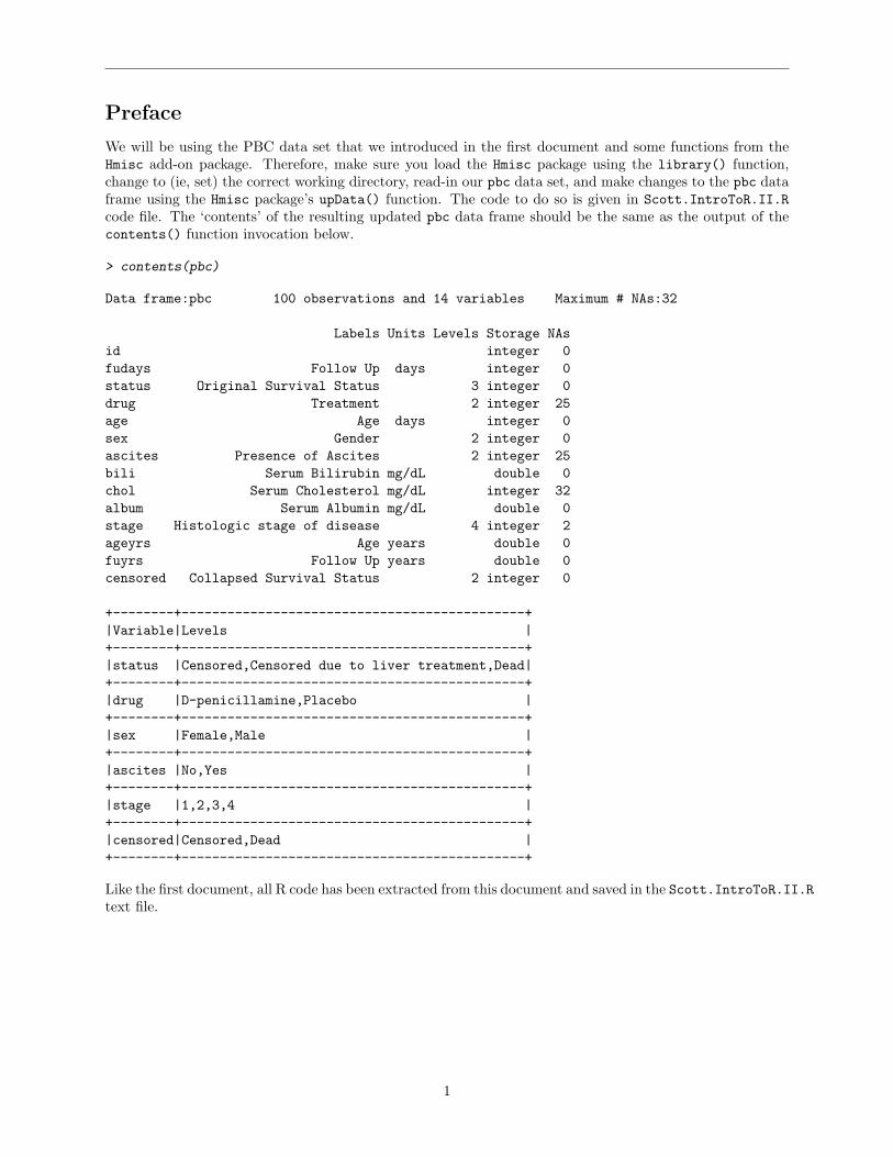
We will be using the PBC data set that we introduced in the first document and some functions from theHmisc add-on package. Therefore, make sure you load the Hmisc package using the library() function,change to (ie, set) the correct working directory, read-in our pbc data set, and make changes to the pbc dataframe using the Hmisc package’s upData() function. The code to do so is given in Scott.IntroToR.II.Rcode file. The ‘contents’ of the resulting updated pbc data frame should be the same as the output of thecontents() function invocation below.
> contents(pbc)
Data frame:pbc 100 observations and 14 variables Maximum # NAs:32
Labels Units Levels Storage NAsid integer 0fudays Follow Up days integer 0status Original Survival Status 3 integer 0drug Treatment 2 integer 25age Age days integer 0sex Gender 2 integer 0ascites Presence of Ascites 2 integer 25bili Serum Bilirubin mg/dL double 0chol Serum Cholesterol mg/dL integer 32album Serum Albumin mg/dL double 0stage Histologic stage of disease 4 integer 2ageyrs Age years double 0fuyrs Follow Up years double 0censored Collapsed Survival Status 2 integer 0
+--------+---------------------------------------------+|Variable|Levels |+--------+---------------------------------------------+|status |Censored,Censored due to liver treatment,Dead|+--------+---------------------------------------------+|drug |D-penicillamine,Placebo |+--------+---------------------------------------------+|sex |Female,Male |+--------+---------------------------------------------+|ascites |No,Yes |+--------+---------------------------------------------+|stage |1,2,3,4 |+--------+---------------------------------------------+|censored|Censored,Dead |+--------+---------------------------------------------+
Like the first document, all R code has been extracted from this document and saved in the Scott.IntroToR.II.Rtext file.
1
Chapter 1
Working with Data Structures
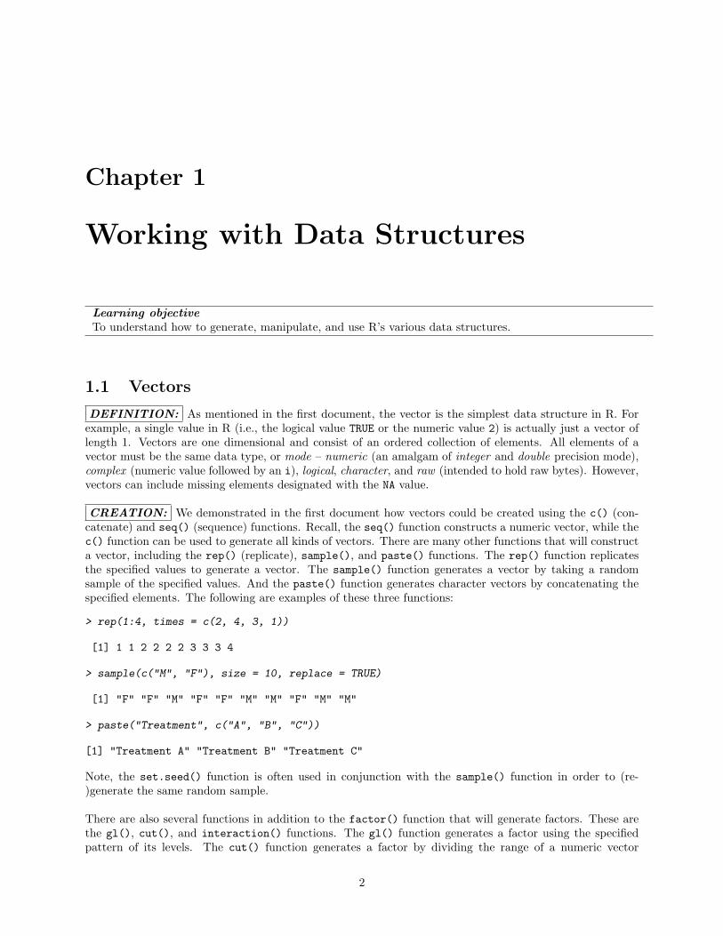
Learning objectiveTo understand how to generate, manipulate, and use R’s various data structures.
1.1 Vectors
DEFINITION: As mentioned in the first document, the vector is the simplest data structure in R. Forexample, a single value in R (i.e., the logical value TRUE or the numeric value 2) is actually just a vector oflength 1. Vectors are one dimensional and consist of an ordered collection of elements. All elements of avector must be the same data type, or mode – numeric (an amalgam of integer and double precision mode),complex (numeric value followed by an i), logical, character, and raw (intended to hold raw bytes). However,vectors can include missing elements designated with the NA value.
CREATION: We demonstrated in the first document how vectors could be created using the c() (con-catenate) and seq() (sequence) functions. Recall, the seq() function constructs a numeric vector, while thec() function can be used to generate all kinds of vectors. There are many other functions that will constructa vector, including the rep() (replicate), sample(), and paste() functions. The rep() function replicatesthe specified values to generate a vector. The sample() function generates a vector by taking a randomsample of the specified values. And the paste() function generates character vectors by concatenating thespecified elements. The following are examples of these three functions:
> rep(1:4, times = c(2, 4, 3, 1))
[1] 1 1 2 2 2 2 3 3 3 4
> sample(c("M", "F"), size = 10, replace = TRUE)
[1] "F" "F" "M" "F" "F" "M" "M" "F" "M" "M"
> paste("Treatment", c("A", "B", "C"))
[1] "Treatment A" "Treatment B" "Treatment C"
Note, the set.seed() function is often used in conjunction with the sample() function in order to (re-)generate the same random sample.
There are also several functions in addition to the factor() function that will generate factors. These arethe gl(), cut(), and interaction() functions. The gl() function generates a factor using the specifiedpattern of its levels. The cut() function generates a factor by dividing the range of a numeric vector
2
CHAPTER 1. WORKING WITH DATA STRUCTURES
into intervals and coding the numeric values according to which interval they fall into. And, as its nameimplies, the interaction() function generates a factor that represents the interaction of the specified levels.The following are examples of these three functions. You’ll notice that we use the levels() function inconjunction with the interaction() function to build a factor from the levels of two existing factors.
> gl(n = 2, k = 8, label = c("Control", "Treatment"))
[1] Control Control Control Control Control Control Control Control[9] Treatment Treatment Treatment Treatment Treatment Treatment Treatment TreatmentLevels: Control Treatment
> head(cut(pbc$ageyrs, breaks = 4))
[1] (54.5,66.5] (30.5,42.5] (54.5,66.5] (42.5,54.5] (30.5,42.5] (54.5,66.5]Levels: (30.5,42.5] (42.5,54.5] (54.5,66.5] (66.5,78.5]
> interaction(levels(pbc$drug), levels(pbc$censored))
[1] D-penicillamine.Censored Placebo.Dead4 Levels: D-penicillamine.Censored Placebo.Censored ... Placebo.Dead
It is also worthwhile to mention character vectors in a little more detail. Specifically, single or double quotescan be embedded in character strings. For example,
> "Single 'quotes' can be embedded in double quotes"
[1] "Single 'quotes' can be embedded in double quotes"
Similarly, double quotes can be embedded into single quote character strings (e.g., ’Example of "double"inside single’), but the single quotes will be converted to double quotes and the embedded double-quoteswill be converted to \". For example, compare the code specified in the Scott.IntroToR.II.R file for thefollowing expression and that shown as output.
> "Double \"quotes\" can be embedded in single quotes"
[1] "Double \"quotes\" can be embedded in single quotes"
In actuality, in order to embed double quotes within a character string specified using double quotes, youmust escape them using a backslash, \. For example,
> "Embedded double quotes, \", must be escaped"
[1] "Embedded double quotes, \", must be escaped"
This \" character specification will make more sense when we discuss functions like as cat() and write.table()in the ‘Data Export’ section.
ATTRIBUTES: All vectors have a length, which is its number of elements and is calculated using thelength() function. For example,
> length(pbc$ageyrs)
[1] 100
However, the length() function does not distinguish missing elements, NAs, from the length of a vector. Forexample, we know that the ascites column of our pbc data frame contains 25 missing values, yet
> length(pbc$ascites)
[1] 100
3
CHAPTER 1. WORKING WITH DATA STRUCTURES
To calculate the number of non-missing elements of a vector, we take advantage of an odd quirk of the logicalvalues, TRUE and FALSE. Specifically, the logical values of TRUE and FALSE are coerced to values of 1 and 0,respectively, when used in arithmetic expressions. So, we can calculate the number of non-missing elementsof a vector using
> sum(!is.na(pbc$ascites))
[1] 75
An alternative is to tabulate the result of the is.na() function using the table() function, as demonstratedin the first document:
> table(!is.na(pbc$ascites))
FALSE TRUE25 75
These same tips can be used with factors.
If the elements of a vector are named, the names() function returns (prints) the associated names. Forexample,
> (x <- c(Dog = "Spot", Horse = "Penny", Cat = "Stripes"))
Dog Horse Cat"Spot" "Penny" "Stripes"
> names(x)
[1] "Dog" "Horse" "Cat"
As mentioned in the first document, the levels() function can be used to return (print) the levels of aspecified factor. Another useful function is the nlevels() function, which returns (prints) the number oflevels of a specified factor. Some examples:
> levels(pbc$stage)
[1] "1" "2" "3" "4"
> nlevels(pbc$stage)
[1] 4
In addition, the mode() function returns (prints) the mode of the specified vector. Recall, all factors arestored internally as integer vectors – more to come in ‘Coercing the mode of a vector’. For example,
> mode(x)
[1] "character"
> mode(pbc$ageyrs)
[1] "numeric"
> mode(pbc$drug)
[1] "numeric"
SUBSETTING: For a vector, we can use single square brackets, [ ], to extract specific subsets of thevector’s elements. Specifically, for a vector x, we use the general form x[index], where index is a vectorthat can be one of the following forms:
4
CHAPTER 1. WORKING WITH DATA STRUCTURES
1. A vector of positive integers. The values in the index vector normally lie in the set 1, 2, ...,length(x). The corresponding elements of the vector are extracted, in that order, to form the result.The index vector can be of any length and the result is of the same length as the index vector.For example, x[6] is the sixth element of x, x[1:10] extracts the first ten elements of x (assuminglength(x) ≥ 10), x[length(x)] extracts the last element of x, and x[c(1, 5, 20)] extracts the1st, 5th, and 20th elements of x (assuming length(x) ≥ 20). We can use any of the functions thatconstruct numeric vectors to define the index vector of positive integers, such as the c() (concatenate),the rep() (replicate), the sample(), and the seq() (sequence) functions or the : (colon) operator. NAis returned if the index vector contains an integer > x, and an empty vector (numeric(0)) is returnedif the index vector contains a 0. Alternatives in this situation are the head() and tail() functions,which will return (print) the first/last n= elements of a vector (n = 6 by default).
2. A vector of negative integers. This specifies the values to be excluded rather than included in theextraction. For example, x[-c(1:5)] extracts all but the first five elements of x – we merely place anegative sign in front of the index vector. As seen, all elements of x except those that are specified inthe index vector are extracted, in their original order, to form the result. The results is the length(x)minus the length of the index vector elements long.
3. A logical vector. In this case, the index vector must be of the same length as x. Values correspondingto TRUE in the index vector are extracted and those corresponding to FALSE or NA are not. The logicalindex vector can be explicitly given (e.g., x[c(TRUE, FALSE, TRUE)]) or can be constructed as aconditional expression using any of the comparison or logic operators – see the vector ’Manipulation’section for more detail. For example,
> set.seed(1)
> (x <- sample(10, size = 10, replace = TRUE))
[1] 3 4 6 10 3 9 10 7 7 1
> x[x == 4]
[1] 4
> x[x > 2 & x < 5]
[1] 3 4 3
As seen, the result is the same length as the number of TRUE values in the index vector. Recall, ifthe vector we are trying to subset contains missing values, we need to make sure our logical indexingvector correctly excludes them using the is.na() function, if desired. For example,
> (x <- c(9, 5, 12, NA, 2, NA, NA, 1))
[1] 9 5 12 NA 2 NA NA 1
> x[x > 2]
[1] 9 5 12 NA NA NA
> x[x > 2 & !is.na(x)]
[1] 9 5 12
An alternative in this situation is the subset() function. You merely specify the vector as its firstargument and a conditional expression as its second. An advantage to the subset() function is thatmissing values are automatically taken as false, so they do not need to be explicitly removed using theis.na() function. For example,
5
CHAPTER 1. WORKING WITH DATA STRUCTURES
> subset(x, x > 2)
[1] 9 5 12
> subset(x, x > 2 & x < 10)
[1] 9 5
4. A vector of character strings. This possibility applies only when the elements of a vector havenames. In that case, a subvector of the names vector may be used in the same way as the positiveintegers case in 1. That is, the strings in the index vector are matched against the names of the elementsof x and the resulting elements are extracted. Alphanumeric names are often easier to remember thannumeric indices of elements. For example,
> (fruit <- c(oranges = 5, bananas = 10, apples = 1, peaches = 30))
oranges bananas apples peaches5 10 1 30
> names(fruit)
[1] "oranges" "bananas" "apples" "peaches"
> fruit[c("apples", "oranges")]
apples oranges1 5
IMPORTANT: As hinted to in the ‘Assignment’ section, extracting elements of a data structure, such asa vector, can be done on the left hand side of an assignment expression (e.g., to select parts of a vector toreplace) as well as on the right-hand side. For example, we can assign the missing values of the x vectorassigned above to zeros:
> x
[1] 9 5 12 NA 2 NA NA 1
> x[is.na(x)] <- 0
> x
[1] 9 5 12 0 2 0 0 1
Note, the recycling rule, discussed in the vector ‘Manipulation’ section, was used in x[!is.na(x)] <- 0.Specifically, the value of 0 was ‘recycled’ to fill in the three missing values of x.
MANIPULATION: Because there are several kinds of vectors, there are many ways in which vectorscan be manipulated. In this document, we will discuss (1) how the vectorization of functions and the re-cycling rule affect vector manipulations; (2) the construction and use of conditional expressions; (3) how tocoerce the mode of a vector; (4) how to construct and manipulate vectors of dates; and (5) how charactervectors can be manipulated using regular expressions.
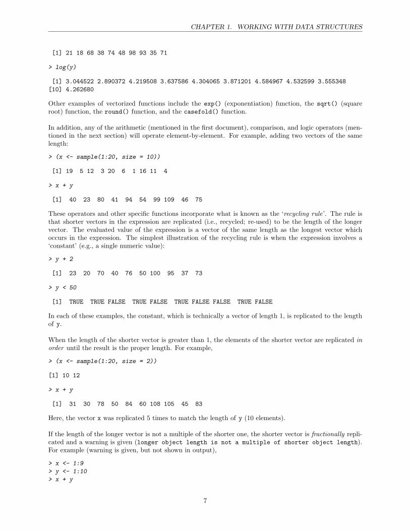
VECTORIZATION OF FUNCTIONS & THE RECYCLING RULE: Many R functions are vectorized, mean-ing that they operate on each of the elements of a vector (i.e., element-by-element). For example, the ex-pression log(y) returns a vector that is the same length of y, where each element of the result is the naturallogarithm of the corresponding element in y.
> (y <- sample(1:100, size = 10))
6
CHAPTER 1. WORKING WITH DATA STRUCTURES
[1] 21 18 68 38 74 48 98 93 35 71
> log(y)
[1] 3.044522 2.890372 4.219508 3.637586 4.304065 3.871201 4.584967 4.532599 3.555348[10] 4.262680
Other examples of vectorized functions include the exp() (exponentiation) function, the sqrt() (squareroot) function, the round() function, and the casefold() function.
In addition, any of the arithmetic (mentioned in the first document), comparison, and logic operators (men-tioned in the next section) will operate element-by-element. For example, adding two vectors of the samelength:
> (x <- sample(1:20, size = 10))
[1] 19 5 12 3 20 6 1 16 11 4
> x + y
[1] 40 23 80 41 94 54 99 109 46 75
These operators and other specific functions incorporate what is known as the ‘recycling rule’. The rule isthat shorter vectors in the expression are replicated (i.e., recycled; re-used) to be the length of the longervector. The evaluated value of the expression is a vector of the same length as the longest vector whichoccurs in the expression. The simplest illustration of the recycling rule is when the expression involves a‘constant’ (e.g., a single numeric value):
> y + 2
[1] 23 20 70 40 76 50 100 95 37 73
> y < 50
[1] TRUE TRUE FALSE TRUE FALSE TRUE FALSE FALSE TRUE FALSE
In each of these examples, the constant, which is technically a vector of length 1, is replicated to the lengthof y.
When the length of the shorter vector is greater than 1, the elements of the shorter vector are replicated inorder until the result is the proper length. For example,
> (x <- sample(1:20, size = 2))
[1] 10 12
> x + y
[1] 31 30 78 50 84 60 108 105 45 83
Here, the vector x was replicated 5 times to match the length of y (10 elements).
If the length of the longer vector is not a multiple of the shorter one, the shorter vector is fractionally repli-cated and a warning is given (longer object length is not a multiple of shorter object length).For example (warning is given, but not shown in output),
> x <- 1:9
> y <- 1:10
> x + y
7
CHAPTER 1. WORKING WITH DATA STRUCTURES
[1] 2 4 6 8 10 12 14 16 18 11
Here, to match the length of y only the first element of x (1) was re-used.
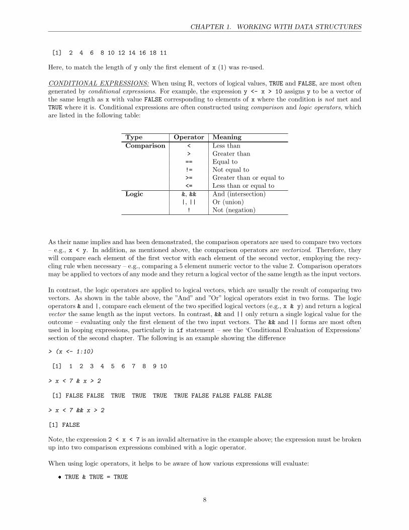
CONDITIONAL EXPRESSIONS: When using R, vectors of logical values, TRUE and FALSE, are most oftengenerated by conditional expressions. For example, the expression y <- x > 10 assigns y to be a vector ofthe same length as x with value FALSE corresponding to elements of x where the condition is not met andTRUE where it is. Conditional expressions are often constructed using comparison and logic operators, whichare listed in the following table:
Type Operator MeaningComparison < Less than
> Greater than== Equal to!= Not equal to>= Greater than or equal to<= Less than or equal to
Logic &, && And (intersection)|, || Or (union)! Not (negation)
As their name implies and has been demonstrated, the comparison operators are used to compare two vectors– e.g., x < y. In addition, as mentioned above, the comparison operators are vectorized. Therefore, theywill compare each element of the first vector with each element of the second vector, employing the recy-cling rule when necessary – e.g., comparing a 5 element numeric vector to the value 2. Comparison operatorsmay be applied to vectors of any mode and they return a logical vector of the same length as the input vectors.
In contrast, the logic operators are applied to logical vectors, which are usually the result of comparing twovectors. As shown in the table above, the ”And” and ”Or” logical operators exist in two forms. The logicoperators & and |, compare each element of the two specified logical vectors (e.g., x & y) and return a logicalvector the same length as the input vectors. In contrast, && and || only return a single logical value for theoutcome – evaluating only the first element of the two input vectors. The && and || forms are most oftenused in looping expressions, particularly in if statement – see the ‘Conditional Evaluation of Expressions’section of the second chapter. The following is an example showing the difference
> (x <- 1:10)
[1] 1 2 3 4 5 6 7 8 9 10
> x < 7 & x > 2
[1] FALSE FALSE TRUE TRUE TRUE TRUE FALSE FALSE FALSE FALSE
> x < 7 && x > 2
[1] FALSE
Note, the expression 2 < x < 7 is an invalid alternative in the example above; the expression must be brokenup into two comparison expressions combined with a logic operator.
When using logic operators, it helps to be aware of how various expressions will evaluate:
TRUE & TRUE = TRUE
8
CHAPTER 1. WORKING WITH DATA STRUCTURES
TRUE & FALSE = FALSE
FALSE & FALSE = FALSE
TRUE | TRUE = TRUE
TRUE | FALSE= TRUE
FALSE | FALSE = FALSE
How various expressions will evaluate becomes a little more tricky when NAs are involved:
NA & TRUE = NA
NA | TRUE = TRUE
NA & FALSE = FALSE
NA | FALSE = NA
Other useful operators include the %in% and the (Hmisc package’s) %nin% value matching operators. Thesebinary operators return a logical vector indicating whether elements of the vector specified as the left operandmatch any of the values in the vector specified as the right operand. The %nin% operator is the ‘negative’ ofthe %in% operator. For example,
> (x <- sample(c("A", "B", "C", "D"), size = 10, replace = TRUE))
[1] "B" "A" "D" "C" "D" "A" "C" "B" "D" "C"
> x %in% c("A", "C", "D")
[1] FALSE TRUE TRUE TRUE TRUE TRUE TRUE FALSE TRUE TRUE
> x %nin% c("A", "B")
[1] FALSE FALSE TRUE TRUE TRUE FALSE TRUE FALSE TRUE TRUE
These operators are useful as alternatives to multiple ‘Or’ statements. For example, x %in% c("A", "C","D") is equivalent to x == "A" | x == "C" | x == "D". Also, to use the %nin% operator, DON’T FOR-GET to load the Hmisc package with the library() function (i.e., library(Hmisc)) if you haven’t alreadydone so. If you haven’t previously installed the package, you must do this first.
To ‘wholly’ compare two vectors, two functions are available: the identical() and all.equal() functions.Some examples:
> x <- 1:3
> y <- 1:3
> x == y
[1] TRUE TRUE TRUE
> identical(x, y)
[1] TRUE
> all.equal(x, y)
[1] TRUE
9
CHAPTER 1. WORKING WITH DATA STRUCTURES
The identical() function compares the internal representation of the data and returns TRUE if the objectsare strictly identical, and FALSE otherwise. On the other hand, the all.equal() function compares the‘near equality’ of two objects, and returns TRUE or displays a summary of the differences. The ‘near equality’arises from the fact that the all.equal() function takes the approximation of the computing process intoaccount when comparing numeric values. The comparison of numeric values on a computer is sometimessurprising! For example,
> 0.9 == (1 - 0.1)
[1] TRUE
> identical(0.9, 1 - 0.1)
[1] TRUE
> all.equal(0.9, 1 - 0.1)
[1] TRUE
> 0.9 == (1.1 - 0.2)
[1] FALSE
> identical(0.9, 1.1 - 0.2)
[1] FALSE
> all.equal(0.9, 1.1 - 0.2)
[1] TRUE
> all.equal(0.9, 1.1 - 0.2, tolerance = 1e-16)
[1] "Mean relative difference: 1.233581e-16"
COERCING THE MODE OF A VECTOR: We’ve mentioned thus far that logical vectors may be used inarithmetic expressions, in which case they are coerced into numeric vectors – FALSE becoming 0 and TRUEbecoming 1. For example,
> x <- c(34, 31, 80, 78, 64, 87)
> x > 35
[1] FALSE FALSE TRUE TRUE TRUE TRUE
> sum(x > 35)
[1] 4
> sum(x > 35)/length(x)
[1] 0.6666667
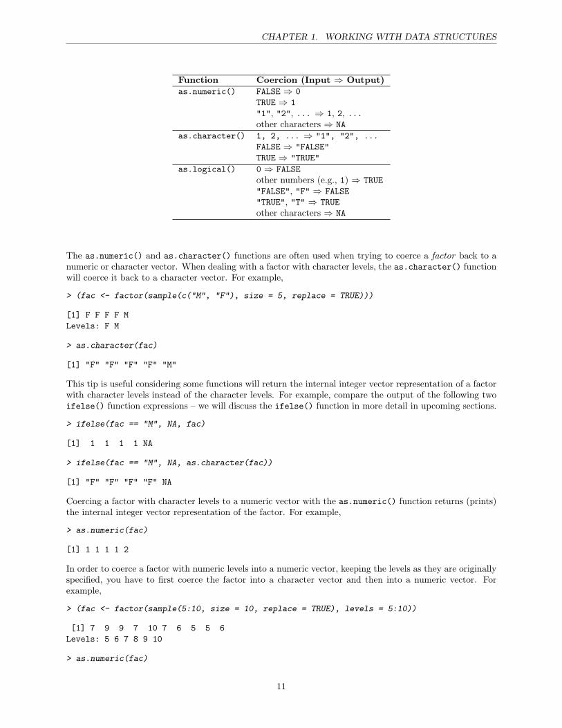
In fact, it is possible to coerce a vector of any mode to any other mode, even though the result may notbe what you wish. These coercions are possible using the many as.X() vector functions in R – in fact,there are many as.X() functions that convert other data structures, but they will only be mentioned in the‘Catalog’ chapter. Even though there are many such as.X() functions for coercing vectors, I have found thatI primarily use just three of them – the as.numeric(), the as.character(), and as.logical() functions,which convert vectors to mode numeric, character, and logical, respectively. Even though the idea of thecoercion follows intuitive rules, the results of the three functions depend on the mode of the input vector, assummarized in the following table:
10
CHAPTER 1. WORKING WITH DATA STRUCTURES
Function Coercion (Input ⇒ Output)as.numeric() FALSE ⇒ 0
TRUE ⇒ 1"1", "2", ... ⇒ 1, 2, ...other characters ⇒ NA
as.character() 1, 2, ... ⇒ "1", "2", ...FALSE ⇒ "FALSE"TRUE ⇒ "TRUE"
as.logical() 0 ⇒ FALSEother numbers (e.g., 1) ⇒ TRUE"FALSE", "F" ⇒ FALSE"TRUE", "T" ⇒ TRUEother characters ⇒ NA
The as.numeric() and as.character() functions are often used when trying to coerce a factor back to anumeric or character vector. When dealing with a factor with character levels, the as.character() functionwill coerce it back to a character vector. For example,
> (fac <- factor(sample(c("M", "F"), size = 5, replace = TRUE)))
[1] F F F F MLevels: F M
> as.character(fac)
[1] "F" "F" "F" "F" "M"
This tip is useful considering some functions will return the internal integer vector representation of a factorwith character levels instead of the character levels. For example, compare the output of the following twoifelse() function expressions – we will discuss the ifelse() function in more detail in upcoming sections.
> ifelse(fac == "M", NA, fac)
[1] 1 1 1 1 NA
> ifelse(fac == "M", NA, as.character(fac))
[1] "F" "F" "F" "F" NA
Coercing a factor with character levels to a numeric vector with the as.numeric() function returns (prints)the internal integer vector representation of the factor. For example,
> as.numeric(fac)
[1] 1 1 1 1 2
In order to coerce a factor with numeric levels into a numeric vector, keeping the levels as they are originallyspecified, you have to first coerce the factor into a character vector and then into a numeric vector. Forexample,
> (fac <- factor(sample(5:10, size = 10, replace = TRUE), levels = 5:10))
[1] 7 9 9 7 10 7 6 5 5 6Levels: 5 6 7 8 9 10
> as.numeric(fac)
11
CHAPTER 1. WORKING WITH DATA STRUCTURES
[1] 3 5 5 3 6 3 2 1 1 2
> as.numeric(as.character(fac))
[1] 7 9 9 7 10 7 6 5 5 6
DATES: We often deal with data in form of a date and/or time, such as a date of birth, procedure, or death.In turn, we often wish to manipulate these date/time fields to calculate values such as the time to deathfrom baseline or the time between treatment visits. Luckily, there are two main ‘datetime’ classes in R’sbase package – Date and POSIX. The Date class supports dates without times. As mentioned in the ‘R HelpDesk’ article of the June 2004 R Newsletter, ‘eliminating times simplifies dates substantially since not onlyare times, themselves, eliminated but the potential complications of time zones and daylight savings time vs.standard time need not be considered either.’ The POSIX class actually refers to the two classes of POSIXctand POSIXlt. It also refers to a POSIXt class, which is the superclass of POSIXct and POSIXlt. Normally wewill not access the POSIXt class directly when using R, but any POSIXlt and POSIXct class specific methodsof generic functions will be given under POSIXt. The POSIXct and POSIXlt classes support times and datesincluding times zones and standard vs. daylight savings time. POSIXct datetimes are represented as thenumber of seconds since January 1, 1970 GMT, while POSIXlt datetimes are represented by a list (‘lt’) of9 components plus an optional timezone attribute. The Date class and POSIXct/POSIXlt classes have asimilar interface, making it easy to move between them.
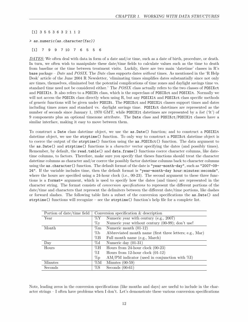
To construct a Date class datetime object, we use the as.Date() function; and to construct a POSIXltdatetime object, we use the strptime() function. To only way to construct a POSIXct datetime object isto coerce the output of the strptime() function using the as.POSIXct() function. The data argument tothe as.Date() and strptime() functions is a character vector specifying the dates (and possibly times).Remember, by default, the read.table() and data.frame() functions coerce character columns, like date-time columns, to factors. Therefore, make sure you specify that theses functions should treat the characterdatetime columns as character and/or coerce the possibly factor datetime columns back to character columnsusing the as.character() function. The default format of the date is "year-month-day", such as "2007-09-24". If the variable includes time, then the default format is "year-month-day hour:minutes:seconds",where the hours are specified using a 24-hour clock (i.e., 00-23). The second argument to these three func-tions is a format= argument, which is used to specify how the dates (and times) are represented in thecharacter string. The format consists of conversion specifications to represent the different portions of thedate/time and characters that represent the delimiters between the different date/time portions, like dashesor forward slashes. The following table lists a subset of the conversion specifications the as.Date() andstrptime() functions will recognize – see the strptime() function’s help file for a complete list.
Portion of date/time field Conversion specification & descriptionYear %Y Numeric year with century (e.g., 2007)
%y Numeric year without century (00-99); don’t use!Month %m Numeric month (01-12)
%b Abbreviated month name (first three letters; e.g., Mar)%B Full month name (e.g., March)
Day %d Numeric day (01-31)Hours %H Hours from 24-hour clock (00-23)
%I Hours from 12-hour clock (01-12)%p AM/PM indicator (used in conjunction with %I)
Minutes %M Minutes (00-59)Seconds %S Seconds (00-61)
Note, leading zeros in the conversion specifications (like months and days) are useful to include in the char-acter strings – I often have problems when I don’t. Let’s demonstrate these various conversion specifications
12
CHAPTER 1. WORKING WITH DATA STRUCTURES
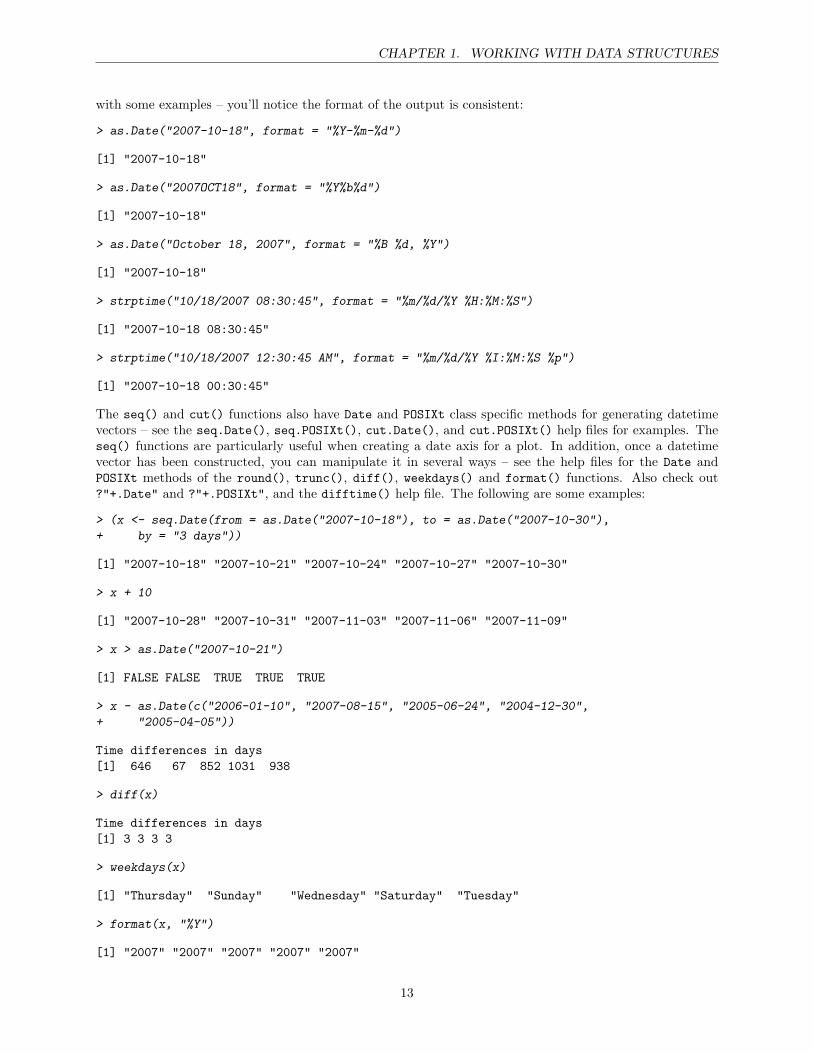
with some examples – you’ll notice the format of the output is consistent:
> as.Date("2007-10-18", format = "%Y-%m-%d")
[1] "2007-10-18"
> as.Date("2007OCT18", format = "%Y%b%d")
[1] "2007-10-18"
> as.Date("October 18, 2007", format = "%B %d, %Y")
[1] "2007-10-18"
> strptime("10/18/2007 08:30:45", format = "%m/%d/%Y %H:%M:%S")
[1] "2007-10-18 08:30:45"
> strptime("10/18/2007 12:30:45 AM", format = "%m/%d/%Y %I:%M:%S %p")
[1] "2007-10-18 00:30:45"
The seq() and cut() functions also have Date and POSIXt class specific methods for generating datetimevectors – see the seq.Date(), seq.POSIXt(), cut.Date(), and cut.POSIXt() help files for examples. Theseq() functions are particularly useful when creating a date axis for a plot. In addition, once a datetimevector has been constructed, you can manipulate it in several ways – see the help files for the Date andPOSIXt methods of the round(), trunc(), diff(), weekdays() and format() functions. Also check out?"+.Date" and ?"+.POSIXt", and the difftime() help file. The following are some examples:
> (x <- seq.Date(from = as.Date("2007-10-18"), to = as.Date("2007-10-30"),
+ by = "3 days"))
[1] "2007-10-18" "2007-10-21" "2007-10-24" "2007-10-27" "2007-10-30"
> x + 10
[1] "2007-10-28" "2007-10-31" "2007-11-03" "2007-11-06" "2007-11-09"
> x > as.Date("2007-10-21")
[1] FALSE FALSE TRUE TRUE TRUE
> x - as.Date(c("2006-01-10", "2007-08-15", "2005-06-24", "2004-12-30",
+ "2005-04-05"))
Time differences in days[1] 646 67 852 1031 938
> diff(x)
Time differences in days[1] 3 3 3 3
> weekdays(x)
[1] "Thursday" "Sunday" "Wednesday" "Saturday" "Tuesday"
> format(x, "%Y")
[1] "2007" "2007" "2007" "2007" "2007"
13

CHAPTER 1. WORKING WITH DATA STRUCTURES
> format(x, "%m/%d/%Y")
[1] "10/18/2007" "10/21/2007" "10/24/2007" "10/27/2007" "10/30/2007"
It is important to mention that you will receive an error if you try to define a new column of a data frame asthe output of the strptime() function. For example, you would receive an error if you invoked an expressionsimilar to df$visitdate <- with(df, strptime(visit, format = "%Y-%m-%d")), where df is a fictitiousdata frame with visit being a character column giving the visit dates. This error will occur because, as wementioned, the strptime() function returns a list, even though it does not appear this way (even if we lookat the structure of the output using the str() function). The remedy to this problem is the above-mentionedas.POSIXct() function, which will coerce the strptime() function output to a datetime vector. Therefore,we should modify the example code to: df$visitdate <- with(df, as.POSIXct(strptime(visit, for-mat = "%Y-%m-%d"))).
In addition to the POSIXct and POSIXlt classes to represent dates and times, there is also the chron package,which is an add-on package available through the CRAN website. The chron package provides dates andtimes, but there are no time zones or notion of daylight vs. standard times. Datetimes in the chron packageare represented internally as days since January 1, 1970, with times represented as fractions of days. Eventhough the chron package includes several functions that allow you to manipulate datetime variables, theformat used to specify the dates and times is not as extensive as the conversion specifications of the POSIXctand POSIXlt classes.
MANIPULATING CHARACTER VECTORS WITH REGULAR EXPRESSIONS: Working with data in Roften involves text data, which are often called character strings. These character strings may be the valuesof a column in a data frame or may be the output from a function like the names() function. In any case, weoften want to extract or manipulate elements of character vectors that match a specific pattern of characters.In R, this is possible using the grep() and sub() functions, respectively, and regular expressions. In general,regular expressions are used to match patterns against character strings. In other words, regular expressionsare special strings of characters that you create in order to locate matching pieces of text. In order tounderstand the power of regular expressions, let’s work through their use with the grep() function, whichsearches for matches to a pattern=, which is specified as its first argument, within the character vector x=,which is specified as its second argument. More information is available regarding regular expressions in theregex help file (ie, ?regex).
Patterns: As we have indicated, every regular expression contains a pattern, which is used to match theregular expression against a character string. Within a pattern, all characters except ., |, (, ), [, ], , , +,\, ^, $, *, and ? match themselves. For example, we could extract the column names of our pbc data framethat contain the character string "age" using the grep() function. Note, we need to also specify value= TRUE in our grep() function expression to return (print) the matching values – by default, the grep()function returns the indices of the matches (value = FALSE).
> names(pbc)
[1] "id" "fudays" "status" "drug" "age" "sex" "ascites"[8] "bili" "chol" "album" "stage" "ageyrs" "fuyrs" "censored"
> grep(pattern = "age", x = names(pbc), value = TRUE)
[1] "age" "stage" "ageyrs"
If you want to match one of the special characters mentioned above literally, you have to precede it withtwo backslashes. For example, we could extract the elements of the following character vector that containa period.
> (char <- c("id", "patient.age", "date", "baseline_bmi", "follow.up.visit"))
14
CHAPTER 1. WORKING WITH DATA STRUCTURES
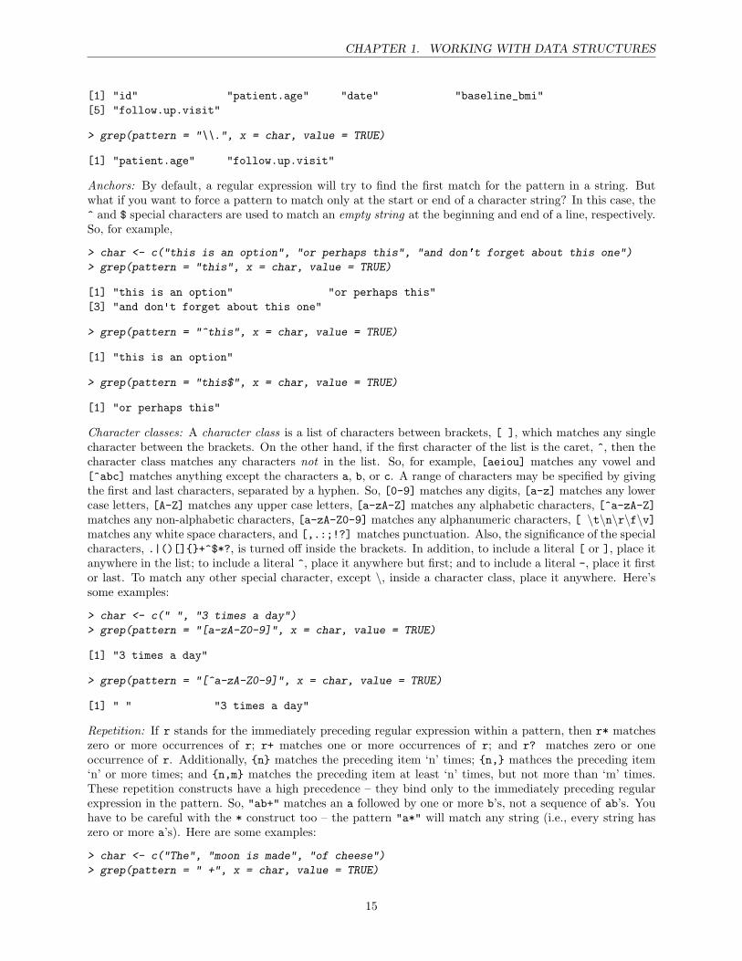
[1] "id" "patient.age" "date" "baseline_bmi"[5] "follow.up.visit"
> grep(pattern = "\\.", x = char, value = TRUE)
[1] "patient.age" "follow.up.visit"
Anchors: By default, a regular expression will try to find the first match for the pattern in a string. Butwhat if you want to force a pattern to match only at the start or end of a character string? In this case, the^ and $ special characters are used to match an empty string at the beginning and end of a line, respectively.So, for example,
> char <- c("this is an option", "or perhaps this", "and don't forget about this one")
> grep(pattern = "this", x = char, value = TRUE)
[1] "this is an option" "or perhaps this"[3] "and don't forget about this one"
> grep(pattern = "^this", x = char, value = TRUE)
[1] "this is an option"
> grep(pattern = "this$", x = char, value = TRUE)
[1] "or perhaps this"
Character classes: A character class is a list of characters between brackets, [ ], which matches any singlecharacter between the brackets. On the other hand, if the first character of the list is the caret, ^, then thecharacter class matches any characters not in the list. So, for example, [aeiou] matches any vowel and[^abc] matches anything except the characters a, b, or c. A range of characters may be specified by givingthe first and last characters, separated by a hyphen. So, [0-9] matches any digits, [a-z] matches any lowercase letters, [A-Z] matches any upper case letters, [a-zA-Z] matches any alphabetic characters, [^a-zA-Z]matches any non-alphabetic characters, [a-zA-Z0-9] matches any alphanumeric characters, [ \t\n\r\f\v]matches any white space characters, and [,.:;!?] matches punctuation. Also, the significance of the specialcharacters, .|()[]+^$*?, is turned off inside the brackets. In addition, to include a literal [ or ], place itanywhere in the list; to include a literal ^, place it anywhere but first; and to include a literal -, place it firstor last. To match any other special character, except \, inside a character class, place it anywhere. Here’ssome examples:
> char <- c(" ", "3 times a day")
> grep(pattern = "[a-zA-Z0-9]", x = char, value = TRUE)
[1] "3 times a day"
> grep(pattern = "[^a-zA-Z0-9]", x = char, value = TRUE)
[1] " " "3 times a day"
Repetition: If r stands for the immediately preceding regular expression within a pattern, then r* matcheszero or more occurrences of r; r+ matches one or more occurrences of r; and r? matches zero or oneoccurrence of r. Additionally, n matches the preceding item ‘n’ times; n, mathces the preceding item‘n’ or more times; and n,m matches the preceding item at least ‘n’ times, but not more than ‘m’ times.These repetition constructs have a high precedence – they bind only to the immediately preceding regularexpression in the pattern. So, "ab+" matches an a followed by one or more b’s, not a sequence of ab’s. Youhave to be careful with the * construct too – the pattern "a*" will match any string (i.e., every string haszero or more a’s). Here are some examples:
> char <- c("The", "moon is made", "of cheese")
> grep(pattern = " +", x = char, value = TRUE)
15

CHAPTER 1. WORKING WITH DATA STRUCTURES
[1] "moon is made" "of cheese"
> grep(pattern = "o?o", x = char, value = TRUE)
[1] "moon is made" "of cheese"
Alternation: The vertical bar, | is a special character because an unescaped vertical bar matches either theregular expression that precedes it or the regular expression that follows it. For example,
> char <- c("red", "ball", "blue", "sky")
> grep(pattern = "d|e", x = char, value = TRUE)
[1] "red" "blue"
> grep(pattern = "al|lu", x = char, value = TRUE)
[1] "ball" "blue"
Grouping: You can use parentheses to group terms within a regular expression. Everything written withinthe group is treated as a single regular expression. For example,
> char <- c("red ball", "blue ball", "red sky", "blue sky")
> grep(pattern = "red", x = char, value = TRUE)
[1] "red ball" "red sky"
> grep(pattern = "(red ball)", x = char, value = TRUE)
[1] "red ball"
We should also mention what the period, ., special character does. An unescaped period, ., matches anysingle character. In addition, the grep() function is case-sensitive – its ignore.case= argument is by defaultFALSE. For example,
> char <- c("vit E", "vitamin e")
> grep(pattern = "vit.*E", x = char, value = TRUE)
[1] "vit E"
> grep(pattern = "vit.*E", x = char, value = TRUE, ignore.case = TRUE)
[1] "vit E" "vitamin e"
As I mentioned above, the sub() (substitute) function also employs regular expressions. The sub() functionneeds a pattern= and x= argument like the grep() function, but it also needs a replacement= argument,which specifies the substitution for the matched pattern. For example,
> char <- c("one.period", "two..periods", "three...periods")
> sub(pattern = "\\.+", replacement = ".", x = char)
[1] "one.period" "two.periods" "three.periods"
With the sub() function, the parentheses take on an additional ability. Specifically, the parentheses can beused to tag a portion of the match as a ‘variable’ to return. For example, we can extract just the leadingnumber from each element of the following character vector.
> char <- c("45: Received chemo", "1, Got too sick", "2; Moved to another hospital")
> sub(pattern = "^([0-9]+)[:,;].*$", "\\1", char)
[1] "45" "1" "2"
16
CHAPTER 1.
Here’s another example:
> char <- c("vit E", "vitamin E", "vitamin ESTER-C", "vit E ")
> sub(pattern = "^(vit).*([E]).*$", "\\1 \\2", char)
[1] "vit E" "vit E" "vit E" "vit E"
It is also worthwhile to mention the gsub() function. Unlike the sub() function, which replaces only thefirst occurrence of a ‘pattern’, the gsub() function replaces all occurrences. For ezample,
> sub(" a", " A", "Capitalizing all words beginning with an a")
[1] "Capitalizing All words beginning with an a"
> gsub(" a", " A", "Capitalizing all words beginning with an a")
[1] "Capitalizing All words beginning with An A"
1.2 Matrices & Arrays
DEFINITION: A matrix is a two-dimensional data structure that consists of rows and columns – thinkof a vector with dimensions. Like vectors, all the elements of a matrix must be the same data type (allnumeric, character, or logical), and can include missing elements designated with the NA value. Taking it onestep further, an array is a generalization of a matrix, which allows more than two dimensions. In general,an array is k -dimensional.
CREATION: To create a matrix, we can use the matrix() function, which constructs an nrow x ncolmatrix from a supplied vector (data=).
> args(matrix)
function (data = NA, nrow = 1, ncol = 1, byrow = FALSE, dimnames = NULL)NULL
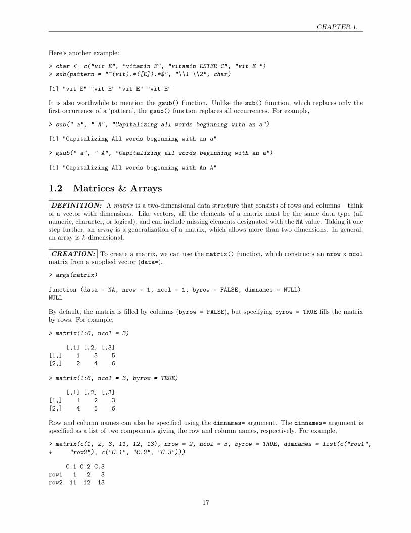
By default, the matrix is filled by columns (byrow = FALSE), but specifying byrow = TRUE fills the matrixby rows. For example,
> matrix(1:6, ncol = 3)
[,1] [,2] [,3][1,] 1 3 5[2,] 2 4 6
> matrix(1:6, ncol = 3, byrow = TRUE)
[,1] [,2] [,3][1,] 1 2 3[2,] 4 5 6
Row and column names can also be specified using the dimnames= argument. The dimnames= argument isspecified as a list of two components giving the row and column names, respectively. For example,
> matrix(c(1, 2, 3, 11, 12, 13), nrow = 2, ncol = 3, byrow = TRUE, dimnames = list(c("row1",
+ "row2"), c("C.1", "C.2", "C.3")))
C.1 C.2 C.3row1 1 2 3row2 11 12 13
17
CHAPTER 1.
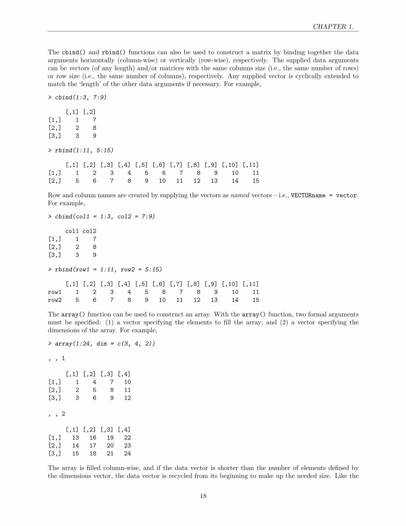
The cbind() and rbind() functions can also be used to construct a matrix by binding together the dataarguments horizontally (column-wise) or vertically (row-wise), respectively. The supplied data argumentscan be vectors (of any length) and/or matrices with the same columns size (i.e., the same number of rows)or row size (i.e., the same number of columns), respectively. Any supplied vector is cyclically extended tomatch the ‘length’ of the other data arguments if necessary. For example,
> cbind(1:3, 7:9)
[,1] [,2][1,] 1 7[2,] 2 8[3,] 3 9
> rbind(1:11, 5:15)
[,1] [,2] [,3] [,4] [,5] [,6] [,7] [,8] [,9] [,10] [,11][1,] 1 2 3 4 5 6 7 8 9 10 11[2,] 5 6 7 8 9 10 11 12 13 14 15
Row and column names are created by supplying the vectors as named vectors – i.e., VECTORname = vector.For example,
> cbind(col1 = 1:3, col2 = 7:9)
col1 col2[1,] 1 7[2,] 2 8[3,] 3 9
> rbind(row1 = 1:11, row2 = 5:15)
[,1] [,2] [,3] [,4] [,5] [,6] [,7] [,8] [,9] [,10] [,11]row1 1 2 3 4 5 6 7 8 9 10 11row2 5 6 7 8 9 10 11 12 13 14 15
The array() function can be used to construct an array. With the array() function, two formal argumentsmust be specified: (1) a vector specifying the elements to fill the array; and (2) a vector specifying thedimensions of the array. For example,
> array(1:24, dim = c(3, 4, 2))
, , 1
[,1] [,2] [,3] [,4][1,] 1 4 7 10[2,] 2 5 8 11[3,] 3 6 9 12
, , 2
[,1] [,2] [,3] [,4][1,] 13 16 19 22[2,] 14 17 20 23[3,] 15 18 21 24
The array is filled column-wise, and if the data vector is shorter than the number of elements defined bythe dimensions vector, the data vector is recycled from its beginning to make up the needed size. Like the
18
CHAPTER 1.
matrix() function, dimension names can be added using the dimnames= argument.
ATTRIBUTES: The dim() function will return (print) the dimensions of the specified matrix or array –the number of rows, columns, etc. If the dimensions of a matrix or array are named (rows, columns, etc), thedimnames() function will return (print) these assigned names. Lastly, because matrices/arrays are similarto vectors in the fact that all of their elements must be the same data type, the mode() function will returnthe mode of the matrix/array.
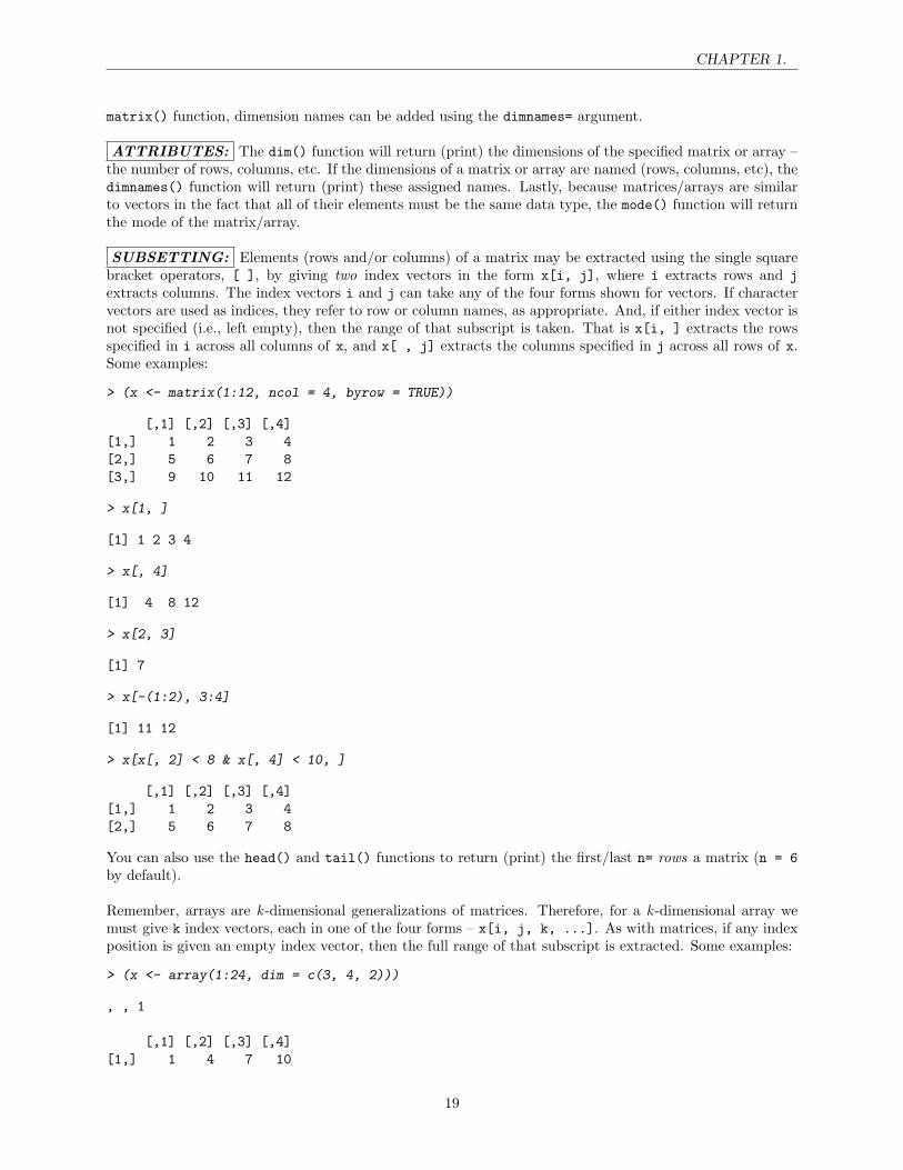
SUBSETTING: Elements (rows and/or columns) of a matrix may be extracted using the single squarebracket operators, [ ], by giving two index vectors in the form x[i, j], where i extracts rows and jextracts columns. The index vectors i and j can take any of the four forms shown for vectors. If charactervectors are used as indices, they refer to row or column names, as appropriate. And, if either index vector isnot specified (i.e., left empty), then the range of that subscript is taken. That is x[i, ] extracts the rowsspecified in i across all columns of x, and x[ , j] extracts the columns specified in j across all rows of x.Some examples:
> (x <- matrix(1:12, ncol = 4, byrow = TRUE))
[,1] [,2] [,3] [,4][1,] 1 2 3 4[2,] 5 6 7 8[3,] 9 10 11 12
> x[1, ]
[1] 1 2 3 4
> x[, 4]
[1] 4 8 12
> x[2, 3]
[1] 7
> x[-(1:2), 3:4]
[1] 11 12
> x[x[, 2] < 8 & x[, 4] < 10, ]
[,1] [,2] [,3] [,4][1,] 1 2 3 4[2,] 5 6 7 8
You can also use the head() and tail() functions to return (print) the first/last n= rows a matrix (n = 6by default).
Remember, arrays are k -dimensional generalizations of matrices. Therefore, for a k -dimensional array wemust give k index vectors, each in one of the four forms – x[i, j, k, ...]. As with matrices, if any indexposition is given an empty index vector, then the full range of that subscript is extracted. Some examples:
> (x <- array(1:24, dim = c(3, 4, 2)))
, , 1
[,1] [,2] [,3] [,4][1,] 1 4 7 10
19
CHAPTER 1.
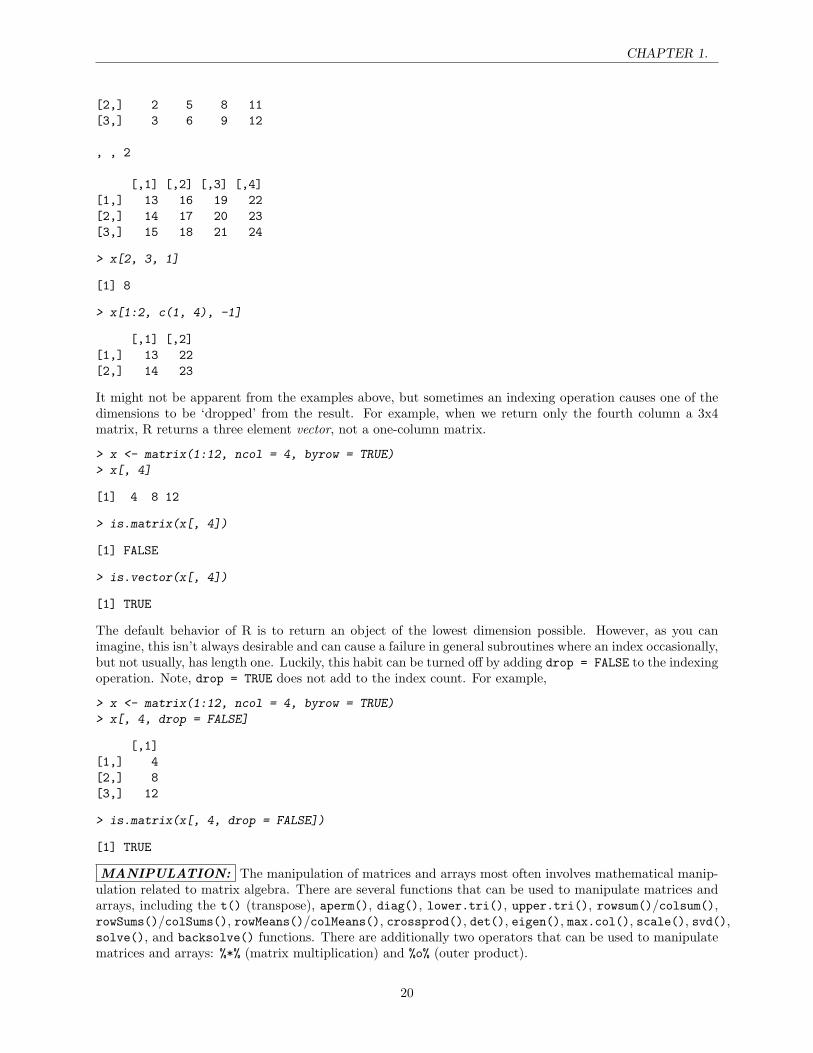
[2,] 2 5 8 11[3,] 3 6 9 12
, , 2
[,1] [,2] [,3] [,4][1,] 13 16 19 22[2,] 14 17 20 23[3,] 15 18 21 24
> x[2, 3, 1]
[1] 8
> x[1:2, c(1, 4), -1]
[,1] [,2][1,] 13 22[2,] 14 23
It might not be apparent from the examples above, but sometimes an indexing operation causes one of thedimensions to be ‘dropped’ from the result. For example, when we return only the fourth column a 3x4matrix, R returns a three element vector, not a one-column matrix.
> x <- matrix(1:12, ncol = 4, byrow = TRUE)
> x[, 4]
[1] 4 8 12
> is.matrix(x[, 4])
[1] FALSE
> is.vector(x[, 4])
[1] TRUE
The default behavior of R is to return an object of the lowest dimension possible. However, as you canimagine, this isn’t always desirable and can cause a failure in general subroutines where an index occasionally,but not usually, has length one. Luckily, this habit can be turned off by adding drop = FALSE to the indexingoperation. Note, drop = TRUE does not add to the index count. For example,
> x <- matrix(1:12, ncol = 4, byrow = TRUE)
> x[, 4, drop = FALSE]
[,1][1,] 4[2,] 8[3,] 12
> is.matrix(x[, 4, drop = FALSE])
[1] TRUE
MANIPULATION: The manipulation of matrices and arrays most often involves mathematical manip-ulation related to matrix algebra. There are several functions that can be used to manipulate matrices andarrays, including the t() (transpose), aperm(), diag(), lower.tri(), upper.tri(), rowsum()/colsum(),rowSums()/colSums(), rowMeans()/colMeans(), crossprod(), det(), eigen(), max.col(), scale(), svd(),solve(), and backsolve() functions. There are additionally two operators that can be used to manipulatematrices and arrays: %*% (matrix multiplication) and %o% (outer product).
20

CHAPTER 1.
1.3 Data frames & Lists
DEFINITION: As defined in the first document, a data frame in R corresponds to what other statisticalpackages call a ‘data matrix’ or a ‘data set’ – the 2-dimensional data structure used to store a completeset of data, which consists of a set of variables (columns) observed on a number of cases (rows). In otherwords, a data frame is a generalization of a matrix. Specifically, the different columns of a data frame maybe of different data types (numeric, character, or logical), but all the elements of any one column must beof the same data type. As with vectors, the elements of any one column can also include missing elementsdesignated with the NA value. Most types of data you will want to read into R and analyze are best describedby data frames.
A list is the most general data structure in R and has the ability to combine a collection of objects intoa larger composite object. Formally, a list in R is a data structure consisting of an ordered collection ofobjects known as its components. Each component can contain any type of R object and the componentsneed not be of the same type. Specifically, a list may contain vectors of several different data types andlengths, matrices or more general arrays, data frames, functions, and/or other lists. Because of this, a listprovides a convenient way to return the results of a computation – in fact, the results that many R functionsreturn are structured as a list, such as the result of fitting a regression model.
It is also important to realize that a data frame is a special case of a list. In fact, a data frame is nothingmore than a list whose components are vectors of the same length and are related in such a way that datain the same ‘position’ come from the same experimental unit (subject, animal, etc.).
CREATION: As demonstrated in the first document, the data.frame() function can be used to constructa data frame from scratch. Often, the data arguments you supply to the data.frame() function will beindividual vectors, which will construct the columns of the data frame. These data arguments can be specifiedwith or without a corresponding column name – either in the form value or the form COLname = value.For example, we can use the sample() function to generate a random data frame.
> ourdf <- data.frame(id = 101:110, sex = sample(c("M", "F"), size = 10,
+ replace = TRUE), age = sample(20:50, size = 10, replace = TRUE),
+ tx = sample(c("Drug", "Placebo"), size = 10, replace = TRUE), diabetes = sample(c(TRUE,
+ FALSE)))
> ourdf
id sex age tx diabetes1 101 F 43 Drug TRUE2 102 F 22 Placebo FALSE3 103 M 47 Placebo TRUE4 104 F 30 Drug FALSE5 105 M 46 Placebo TRUE6 106 M 30 Drug FALSE7 107 M 30 Drug TRUE8 108 F 34 Placebo FALSE9 109 M 47 Drug TRUE10 110 M 46 Placebo FALSE
With the data.frame() function, character vectors are automatically coerced into factors because of itsstringsAsFactors= argument. However, specifying stringsAsFactors = FALSE in your data.frame()function invocation will keep character vectors from being coerced. An alternative is to wrap the charactervector with the I() function, which keeps it ‘as is’. Also, all invalid characters in column names (e.g., spaces,dashes, or question marks) are converted to periods (.).
The list() function can be used to construct a list. Like the data.frame() function, the components of alist can be named using the COMPONENTname = component construct. For example,
21
CHAPTER 1.
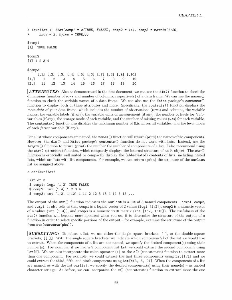
> (ourlist <- list(comp1 = c(TRUE, FALSE), comp2 = 1:4, comp3 = matrix(1:20,
+ nrow = 2, byrow = TRUE)))
$comp1[1] TRUE FALSE
$comp2[1] 1 2 3 4
$comp3[,1] [,2] [,3] [,4] [,5] [,6] [,7] [,8] [,9] [,10]
[1,] 1 2 3 4 5 6 7 8 9 10[2,] 11 12 13 14 15 16 17 18 19 20
ATTRIBUTES: Also as demonstrated in the first document, we can use the dim() function to check thedimensions (number of rows and number of columns, respectively) of a data frame. We can use the names()function to check the variable names of a data frame. We can also use the Hmisc package’s contents()function to display both of these attributes and more. Specifically, the contents() function displays themeta-data of your data frame, which includes the number of observations (rows) and columns, the variablenames, the variable labels (if any), the variable units of measurement (if any), the number of levels for factorvariables (if any), the storage mode of each variable, and the number of missing values (NAs) for each variable.The contents() function also displays the maximum number of NAs across all variables, and the level labelsof each factor variable (if any).
For a list whose components are named, the names() function will return (print) the names of the components.However, the dim() and Hmisc package’s contents() function do not work with lists. Instead, use thelength() function to return (print) the number the number of components of a list. I also recommend usingthe str() (structure) function, which compactly displays the internal structure of an R object. The str()function is especially well suited to compactly display the (abbreviated) contents of lists, including nestedlists, which are lists with list components. For example, we can return (print) the structure of the ourlistlist we assigned above.
> str(ourlist)
List of 3$ comp1: logi [1:2] TRUE FALSE$ comp2: int [1:4] 1 2 3 4$ comp3: int [1:2, 1:10] 1 11 2 12 3 13 4 14 5 15 ...
The output of the str() function indicates the ourlist is a list of 3 named components – comp1, comp2,and comp3. It also tells us that comp1 is a logical vector of 2 values (logi [1:2]), comp2 is a numeric vectorof 4 values (int [1:4]), and comp3 is a numeric 2x10 matrix (int [1:2, 1:10]). The usefulness of thestr() function will become more apparent when you use it to determine the structure of the output of afunction in order to select specific portions of the output – for example, examine the structure of the outputfrom str(contents(pbc)).
SUBSETTING: To subset a list, we use either the single square brackets, [ ], or the double squarebrackets, [[ ]]. With the single square brackets, we indicate which component(s) of the list we would liketo extract. When the components of a list are not named, we specify the desired component(s) using theirnumber(s). For example, if we had a 9 component list Lst we could extract the second component usingLst[2]. We can also incorporate the colon operator (:) or the c() (concatenate) function to extract morethan one component. For example, we could extract the first three components using Lst[1:3] and wecould extract the third, fifth, and ninth components using Lst[c(3, 5, 9)]. When the components of a listare named, as with the list ourlist, we specify the desired component(s) using their name(s) – as quotedcharacter strings. As before, we can incorporate the c() (concatenate) function to extract more the one
22

CHAPTER 1.
named component. For example, we could extract the first component of ourlist using ourlist["comp1"]and we could extract the first and third components using ourlist[c("comp1", "comp3")].
IMPORTANT: Subsetting a list using the single square brackets, [], returns a list ! Therefore, the resultis a sublist of the original list, consisting of the specified components. If it was a named list, the names aretransferred to the sublist. For example,
> str(ourlist["comp1"])
List of 1$ comp1: logi [1:2] TRUE FALSE
In contrast, subsetting a list using the double square brackets, [[ ]], extracts the object that was storedin the specified component. Because of this, we specify only a single component to be extracted with thedouble square brackets – we do not incorporate the colon operator, :, or the c() (concatenate) function.Also, the name of the object is not included when it is extracted, if the corresponding component was namedin the list. As with the single square brackets, [ ], the number of the component can be specified using itsnumber or its name, if appropriate. If the components of a list are named, an alternative to the double squarebrackets is the $ operator. Therefore, Lst[["ComponentName"]] is equivalent to Lst$ComponentName. Forexample,
> ourlist[["comp1"]]
[1] TRUE FALSE
> str(ourlist[["comp1"]])
logi [1:2] TRUE FALSE
> ourlist$comp3
[,1] [,2] [,3] [,4] [,5] [,6] [,7] [,8] [,9] [,10][1,] 1 2 3 4 5 6 7 8 9 10[2,] 11 12 13 14 15 16 17 18 19 20
> str(ourlist$comp3)
int [1:2, 1:10] 1 11 2 12 3 13 4 14 5 15 ...
Because the result of subsetting a list using the double square brackets is the stored object, the result canthen be itself subsetted as demonstrated for vectors, matrices, etc. For example, we can extract the thirdcolumn of the comp3 matrix from ourlist using ourlist$comp3[, 3].
Because data frames are a special case of lists, elements (rows and/or columns) of a data frame can beextracted using the [ ], [[ ]], and/or $ operators. In addition, because a data frame can be thought of asa generalization of a matrix, we can also use the [ , ] subsetting format. If df is our data frame and v1,v2, and v3 are its columns, then df[["v1"]], df$v1, and df[, "v1"] are equivalent and they all return avector. However, df["v1"] returns a data frame. Similarly, specifying more than one column with the [ ,] subsetting format returns a data frame. Some examples using the ourdf data frame:
> ourdf[, 4]
[1] Drug Placebo Placebo Drug Placebo Drug Drug Placebo Drug PlaceboLevels: Drug Placebo
> ourdf[["tx"]]
[1] Drug Placebo Placebo Drug Placebo Drug Drug Placebo Drug PlaceboLevels: Drug Placebo
23
CHAPTER 1.
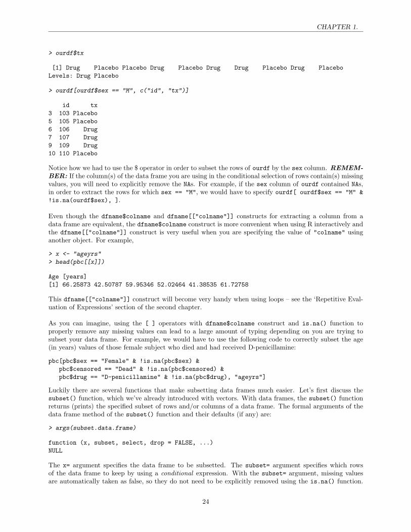
> ourdf$tx
[1] Drug Placebo Placebo Drug Placebo Drug Drug Placebo Drug PlaceboLevels: Drug Placebo
> ourdf[ourdf$sex == "M", c("id", "tx")]
id tx3 103 Placebo5 105 Placebo6 106 Drug7 107 Drug9 109 Drug10 110 Placebo
Notice how we had to use the $ operator in order to subset the rows of ourdf by the sex column. REMEM-BER: If the column(s) of the data frame you are using in the conditional selection of rows contain(s) missingvalues, you will need to explicitly remove the NAs. For example, if the sex column of ourdf contained NAs,in order to extract the rows for which sex == "M", we would have to specify ourdf[ ourdf$sex == "M" &!is.na(ourdf$sex), ].
Even though the dfname$colname and dfname[["colname"]] constructs for extracting a column from adata frame are equivalent, the dfname$colname construct is more convenient when using R interactively andthe dfname[["colname"]] construct is very useful when you are specifying the value of "colname" usinganother object. For example,
> x <- "ageyrs"
> head(pbc[[x]])
Age [years][1] 66.25873 42.50787 59.95346 52.02464 41.38535 61.72758
This dfname[["colname"]] construct will become very handy when using loops – see the ‘Repetitive Eval-uation of Expressions’ section of the second chapter.
As you can imagine, using the [ ] operators with dfname$colname construct and is.na() function toproperly remove any missing values can lead to a large amount of typing depending on you are trying tosubset your data frame. For example, we would have to use the following code to correctly subset the age(in years) values of those female subject who died and had received D-penicillamine:
pbc[pbc$sex == "Female" & !is.na(pbc$sex) &pbc$censored == "Dead" & !is.na(pbc$censored) &pbc$drug == "D-penicillamine" & !is.na(pbc$drug), "ageyrs"]
Luckily there are several functions that make subsetting data frames much easier. Let’s first discuss thesubset() function, which we’ve already introduced with vectors. With data frames, the subset() functionreturns (prints) the specified subset of rows and/or columns of a data frame. The formal arguments of thedata frame method of the subset() function and their defaults (if any) are:
> args(subset.data.frame)
function (x, subset, select, drop = FALSE, ...)NULL
The x= argument specifies the data frame to be subsetted. The subset= argument specifies which rowsof the data frame to keep by using a conditional expression. With the subset= argument, missing valuesare automatically taken as false, so they do not need to be explicitly removed using the is.na() function.
24
CHAPTER 1.
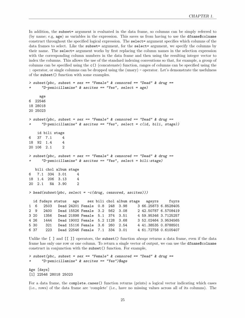
In addition, the subset= argument is evaluated in the data frame, so columns can be simply referred to(by name; e.g, age) as variables in the expression. This saves us from having to use the dfname$colnameconstruct throughout the specified logical expression. The select= argument specifies which columns of thedata frames to select. Like the subset= argument, for the select= argument, we specify the columns bytheir name. The select= argument works by first replacing the column names in the selection expressionwith the corresponding column numbers in the data frame and then using the resulting integer vector toindex the columns. This allows the use of the standard indexing conventions so that, for example, a group ofcolumns can be specified using the c() (concatenate) function, ranges of columns can be specified using the: operator, or single columns can be dropped using the (unary) - operator. Let’s demonstrate the usefulnessof the subset() function with some examples.
> subset(pbc, subset = sex == "Female" & censored == "Dead" & drug ==
+ "D-penicillamine" & ascites == "Yes", select = age)
age6 2254618 2801820 25023
> subset(pbc, subset = sex == "Female" & censored == "Dead" & drug ==
+ "D-penicillamine" & ascites == "Yes", select = c(id, bili, stage))
id bili stage6 37 7.1 418 92 1.4 420 106 2.1 2
> subset(pbc, subset = sex == "Female" & censored == "Dead" & drug ==
+ "D-penicillamine" & ascites == "Yes", select = bili:stage)
bili chol album stage6 7.1 334 3.01 418 1.4 206 3.13 420 2.1 NA 3.90 2
> head(subset(pbc, select = -c(drug, censored, ascites)))
id fudays status age sex bili chol album stage ageyrs fuyrs1 6 2503 Dead 24201 Female 0.8 248 3.98 3 66.25873 6.85284052 9 2400 Dead 15526 Female 3.2 562 3.08 2 42.50787 6.57084193 20 1356 Dead 21898 Female 5.1 374 3.51 4 59.95346 3.71252574 26 1444 Dead 19002 Female 5.2 1128 3.68 3 52.02464 3.95345655 30 321 Dead 15116 Female 3.6 260 2.54 4 41.38535 0.87885016 37 223 Dead 22546 Female 7.1 334 3.01 4 61.72758 0.6105407
Unlike the [ ] and [[ ]] operators, the subset() function always returns a data frame, even if the dataframe has only one row or one column. To return a single vector of output, we can use the dfname$colnameconstruct in conjunction with the subset() function. For example,
> subset(pbc, subset = sex == "Female" & censored == "Dead" & drug ==
+ "D-penicillamine" & ascites == "Yes")$age
Age [days][1] 22546 28018 25023
For a data frame, the complete.cases() function returns (prints) a logical vector indicating which cases(i.e., rows) of the data frame are ‘complete’ (i.e., have no missing values across all of its columns). The
25
CHAPTER 1.
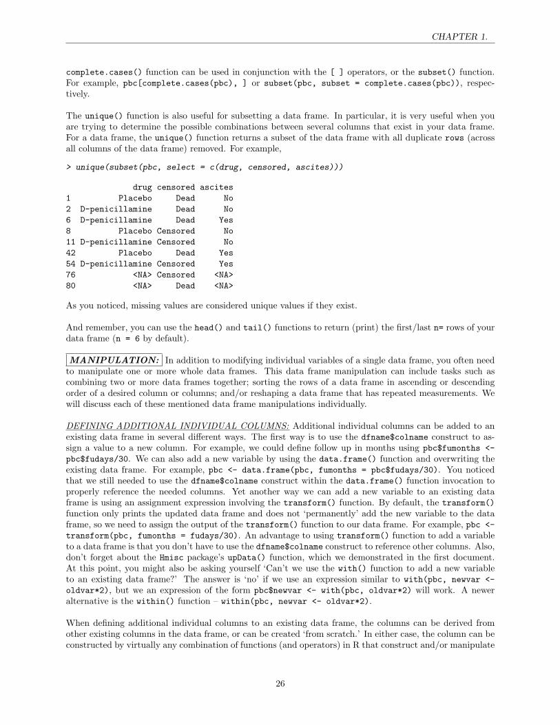
complete.cases() function can be used in conjunction with the [ ] operators, or the subset() function.For example, pbc[complete.cases(pbc), ] or subset(pbc, subset = complete.cases(pbc)), respec-tively.
The unique() function is also useful for subsetting a data frame. In particular, it is very useful when youare trying to determine the possible combinations between several columns that exist in your data frame.For a data frame, the unique() function returns a subset of the data frame with all duplicate rows (acrossall columns of the data frame) removed. For example,
> unique(subset(pbc, select = c(drug, censored, ascites)))
drug censored ascites1 Placebo Dead No2 D-penicillamine Dead No6 D-penicillamine Dead Yes8 Placebo Censored No11 D-penicillamine Censored No42 Placebo Dead Yes54 D-penicillamine Censored Yes76 <NA> Censored <NA>80 <NA> Dead <NA>
As you noticed, missing values are considered unique values if they exist.
And remember, you can use the head() and tail() functions to return (print) the first/last n= rows of yourdata frame (n = 6 by default).
MANIPULATION: In addition to modifying individual variables of a single data frame, you often needto manipulate one or more whole data frames. This data frame manipulation can include tasks such ascombining two or more data frames together; sorting the rows of a data frame in ascending or descendingorder of a desired column or columns; and/or reshaping a data frame that has repeated measurements. Wewill discuss each of these mentioned data frame manipulations individually.
DEFINING ADDITIONAL INDIVIDUAL COLUMNS: Additional individual columns can be added to anexisting data frame in several different ways. The first way is to use the dfname$colname construct to as-sign a value to a new column. For example, we could define follow up in months using pbc$fumonths <-pbc$fudays/30. We can also add a new variable by using the data.frame() function and overwriting theexisting data frame. For example, pbc <- data.frame(pbc, fumonths = pbc$fudays/30). You noticedthat we still needed to use the dfname$colname construct within the data.frame() function invocation toproperly reference the needed columns. Yet another way we can add a new variable to an existing dataframe is using an assignment expression involving the transform() function. By default, the transform()function only prints the updated data frame and does not ‘permanently’ add the new variable to the dataframe, so we need to assign the output of the transform() function to our data frame. For example, pbc <-transform(pbc, fumonths = fudays/30). An advantage to using transform() function to add a variableto a data frame is that you don’t have to use the dfname$colname construct to reference other columns. Also,don’t forget about the Hmisc package’s upData() function, which we demonstrated in the first document.At this point, you might also be asking yourself ‘Can’t we use the with() function to add a new variableto an existing data frame?’ The answer is ‘no’ if we use an expression similar to with(pbc, newvar <-oldvar*2), but we an expression of the form pbc$newvar <- with(pbc, oldvar*2) will work. A neweralternative is the within() function – within(pbc, newvar <- oldvar*2).
When defining additional individual columns to an existing data frame, the columns can be derived fromother existing columns in the data frame, or can be created ‘from scratch.’ In either case, the column can beconstructed by virtually any combination of functions (and operators) in R that construct and/or manipulate
26
CHAPTER 1.
vectors – see the ‘Catalog’ chapter.
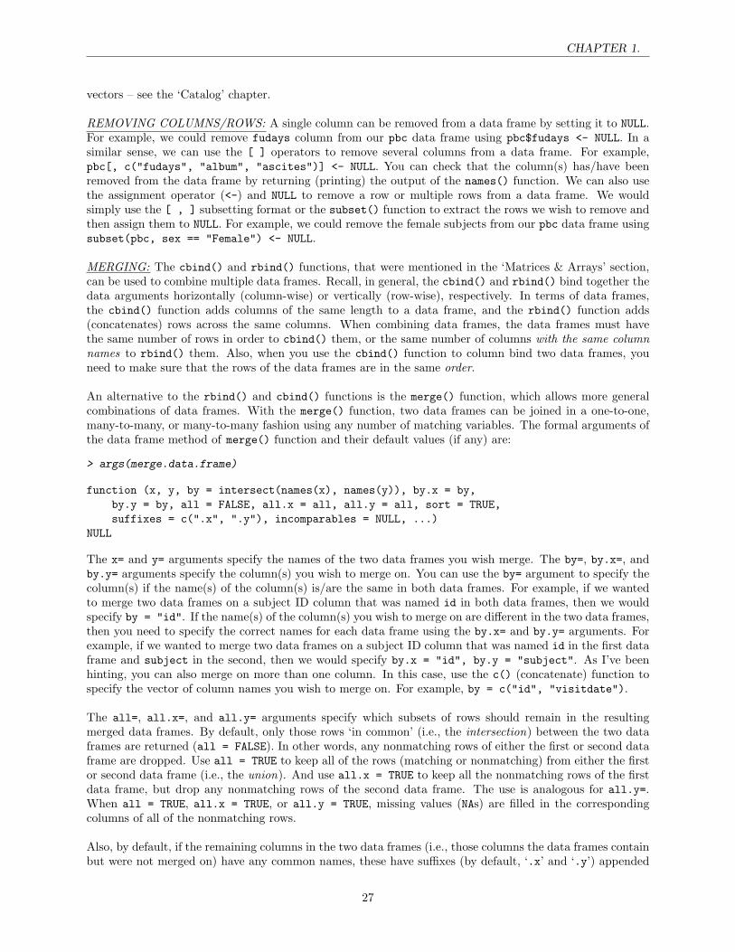
REMOVING COLUMNS/ROWS: A single column can be removed from a data frame by setting it to NULL.For example, we could remove fudays column from our pbc data frame using pbc$fudays <- NULL. In asimilar sense, we can use the [ ] operators to remove several columns from a data frame. For example,pbc[, c("fudays", "album", "ascites")] <- NULL. You can check that the column(s) has/have beenremoved from the data frame by returning (printing) the output of the names() function. We can also usethe assignment operator (<-) and NULL to remove a row or multiple rows from a data frame. We wouldsimply use the [ , ] subsetting format or the subset() function to extract the rows we wish to remove andthen assign them to NULL. For example, we could remove the female subjects from our pbc data frame usingsubset(pbc, sex == "Female") <- NULL.
MERGING: The cbind() and rbind() functions, that were mentioned in the ‘Matrices & Arrays’ section,can be used to combine multiple data frames. Recall, in general, the cbind() and rbind() bind together thedata arguments horizontally (column-wise) or vertically (row-wise), respectively. In terms of data frames,the cbind() function adds columns of the same length to a data frame, and the rbind() function adds(concatenates) rows across the same columns. When combining data frames, the data frames must havethe same number of rows in order to cbind() them, or the same number of columns with the same columnnames to rbind() them. Also, when you use the cbind() function to column bind two data frames, youneed to make sure that the rows of the data frames are in the same order.
An alternative to the rbind() and cbind() functions is the merge() function, which allows more generalcombinations of data frames. With the merge() function, two data frames can be joined in a one-to-one,many-to-many, or many-to-many fashion using any number of matching variables. The formal arguments ofthe data frame method of merge() function and their default values (if any) are:
> args(merge.data.frame)
function (x, y, by = intersect(names(x), names(y)), by.x = by,by.y = by, all = FALSE, all.x = all, all.y = all, sort = TRUE,suffixes = c(".x", ".y"), incomparables = NULL, ...)
NULL
The x= and y= arguments specify the names of the two data frames you wish merge. The by=, by.x=, andby.y= arguments specify the column(s) you wish to merge on. You can use the by= argument to specify thecolumn(s) if the name(s) of the column(s) is/are the same in both data frames. For example, if we wantedto merge two data frames on a subject ID column that was named id in both data frames, then we wouldspecify by = "id". If the name(s) of the column(s) you wish to merge on are different in the two data frames,then you need to specify the correct names for each data frame using the by.x= and by.y= arguments. Forexample, if we wanted to merge two data frames on a subject ID column that was named id in the first dataframe and subject in the second, then we would specify by.x = "id", by.y = "subject". As I’ve beenhinting, you can also merge on more than one column. In this case, use the c() (concatenate) function tospecify the vector of column names you wish to merge on. For example, by = c("id", "visitdate").
The all=, all.x=, and all.y= arguments specify which subsets of rows should remain in the resultingmerged data frames. By default, only those rows ‘in common’ (i.e., the intersection) between the two dataframes are returned (all = FALSE). In other words, any nonmatching rows of either the first or second dataframe are dropped. Use all = TRUE to keep all of the rows (matching or nonmatching) from either the firstor second data frame (i.e., the union). And use all.x = TRUE to keep all the nonmatching rows of the firstdata frame, but drop any nonmatching rows of the second data frame. The use is analogous for all.y=.When all = TRUE, all.x = TRUE, or all.y = TRUE, missing values (NAs) are filled in the correspondingcolumns of all of the nonmatching rows.
Also, by default, if the remaining columns in the two data frames (i.e., those columns the data frames containbut were not merged on) have any common names, these have suffixes (by default, ‘.x’ and ‘.y’) appended
27
CHAPTER 1.
to their names to make the names of the result unique. Use the suffixes= argument to change this default.
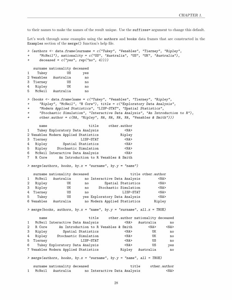
Let’s work through some examples using the authors and books data frames that are constructed in theExamples section of the merge() function’s help file.
> (authors <- data.frame(surname = c("Tukey", "Venables", "Tierney", "Ripley",
+ "McNeil"), nationality = c("US", "Australia", "US", "UK", "Australia"),
+ deceased = c("yes", rep("no", 4))))
surname nationality deceased1 Tukey US yes2 Venables Australia no3 Tierney US no4 Ripley UK no5 McNeil Australia no
> (books <- data.frame(name = c("Tukey", "Venables", "Tierney", "Ripley",
+ "Ripley", "McNeil", "R Core"), title = c("Exploratory Data Analysis",
+ "Modern Applied Statistics", "LISP-STAT", "Spatial Statistics",
+ "Stochastic Simulation", "Interactive Data Analysis", "An Introduction to R"),
+ other.author = c(NA, "Ripley", NA, NA, NA, NA, "Venables & Smith")))
name title other.author1 Tukey Exploratory Data Analysis <NA>2 Venables Modern Applied Statistics Ripley3 Tierney LISP-STAT <NA>4 Ripley Spatial Statistics <NA>5 Ripley Stochastic Simulation <NA>6 McNeil Interactive Data Analysis <NA>7 R Core An Introduction to R Venables & Smith
> merge(authors, books, by.x = "surname", by.y = "name")
surname nationality deceased title other.author1 McNeil Australia no Interactive Data Analysis <NA>2 Ripley UK no Spatial Statistics <NA>3 Ripley UK no Stochastic Simulation <NA>4 Tierney US no LISP-STAT <NA>5 Tukey US yes Exploratory Data Analysis <NA>6 Venables Australia no Modern Applied Statistics Ripley
> merge(books, authors, by.x = "name", by.y = "surname", all.x = TRUE)
name title other.author nationality deceased1 McNeil Interactive Data Analysis <NA> Australia no2 R Core An Introduction to R Venables & Smith <NA> <NA>3 Ripley Spatial Statistics <NA> UK no4 Ripley Stochastic Simulation <NA> UK no5 Tierney LISP-STAT <NA> US no6 Tukey Exploratory Data Analysis <NA> US yes7 Venables Modern Applied Statistics Ripley Australia no
> merge(authors, books, by.x = "surname", by.y = "name", all = TRUE)
surname nationality deceased title other.author1 McNeil Australia no Interactive Data Analysis <NA>
28

CHAPTER 1.
2 Ripley UK no Spatial Statistics <NA>3 Ripley UK no Stochastic Simulation <NA>4 Tierney US no LISP-STAT <NA>5 Tukey US yes Exploratory Data Analysis <NA>6 Venables Australia no Modern Applied Statistics Ripley7 R Core <NA> <NA> An Introduction to R Venables & Smith
In all three merge() function examples, we had to specify by.x= and by.y= because the column names werenot the same in the two data frames (i.e., surname and name). In the first merge, all nonmatching rows ofbooks were dropped from the result (i.e., the row corresponding to name equal R Core). You’ll also noticethat a second row for surname equal Ripley was added to the result to match the two rows for name equalRipley in the books data frame. In the second merge, we specified that the nonmatching rows of the booksdata frame should not be dropped (i.e., the name equal R Core row), and missing values were filled into theremaining columns of the result (nationality and decreased), which came from the authors data frame.In the third merge, all rows from both data frames were kept in the result, and missing values were filledinto the appropriate columns – the nationality and deceased columns for the surname equal R Core row.
SORTING: Even though the sort() function is available to sort the elements of individual vectors, whendealing with data frames, sorting a single vector is not usually what is required. More often, you need tosort a series of columns according to the values of some other columns. For example, we may want to sortthe pbc data frame by treatment (drug), gender (sex), and survival status (censored). With data frames,we also have to make sure that the whole records (single rows across all the columns) are correctly sorted,not just individual columns. To sort data frames, we will want to use the order() function instead of thesort() function. Unlike the sort() function, the order() function can operate on more than one vectorsimultaneously. For example, order(x, y) will return (print) the index vector which rearranges x (its firstargument) into ascending or descending order, with ties broken by y (its second argument). If more thantwo arguments are given, ties are broken by subsequent arguments. By default, all vectors involved in theorder() expression are sorted in ascending order. Because the order() function returns an index vectorand not the original data (like the sort()) function), we use the order() function in conjunction with the[ ] operators to properly sort the rows of a data frame. So, returning to our example, we can sort thepbc data frame by treatment (drug), gender (sex), and survival status (censored) using pbc[with(pbc,order(drug, sex, censored)), ]. We used the with() function to save some typing. When our order()expression involves numeric vectors, we can use the (unary) - operator to specify that a numeric vectorshould be sorted in descending order. For example, we can sort the pbc data frame by treatment (drug),descending age, and survival status (censored) using pbc[with(pbc, order(drug, - age, censored)),].
RESHAPING: Often, your data frame contains repeated measures. For example, perhaps each subject inyour data frame received various kinds of chemotherapy at different visit dates. The reshape() function wascreated to easily manipulate the ‘shape’ of such longitudinal data frames. For the reshape() function, theshape of a data frame can be either ‘wide’ or ‘long.’ A ‘wide’ longitudinal data frame will have one record foreach individual, time-constant variables occupying single columns, and time-varying variables occupying acolumn for each time point. In a ‘long’ format, the data frame will have multiple records for each individual,with some variables being constant across these multiple records and others varying across these multiplerecords. A ‘long’ format data frame also needs a ‘time’ variable identifying which time point each recordcomes from and an ‘id’ variable showing which records refer to the same subject.
So, as its name implies, the reshape() function reshapes data frames between the ‘wide’ and ‘long’ formats.The formal arguments of the reshape() function and their default values (if any) are:
> args(reshape)
function (data, varying = NULL, v.names = NULL, timevar = "time",idvar = "id", ids = 1:NROW(data), times = seq_along(varying[[1]]),drop = NULL, direction, new.row.names = NULL, sep = ".",
29
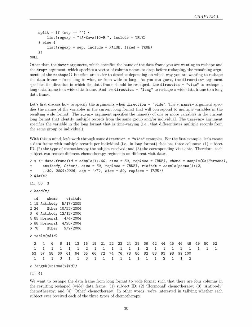
CHAPTER 1.
split = if (sep == "") list(regexp = "[A-Za-z][0-9]", include = TRUE)
else list(regexp = sep, include = FALSE, fixed = TRUE)
)NULL
Other than the data= argument, which specifies the name of the data frame you are wanting to reshape andthe drop= argument, which specifies a vector of column names to drop before reshaping, the remaining argu-ments of the reshape() function are easier to describe depending on which way you are wanting to reshapethe data frame – from long to wide, or from wide to long. As you can guess, the direction= argumentspecifies the direction in which the data frame should be reshaped. Use direction = "wide" to reshape along data frame to a wide data frame. And use direction = "long" to reshape a wide data frame to a longdata frame.
Let’s first discuss how to specify the arguments when direction = "wide". The v.names= argument spec-ifies the names of the variables in the current long format that will correspond to multiple variables in theresulting wide format. The idvar= argument specifies the name(s) of one or more variables in the currentlong format that identify multiple records from the same group and/or individual. The timevar= argumentspecifies the variable in the long format that is time-varying (i.e., that differentiates multiple records fromthe same group or individual).
With this in mind, let’s work through some direction = "wide" examples. For the first example, let’s createa data frame with multiple records per individual (i.e., in long format) that has three columns: (1) subjectID; (2) the type of chemotherapy the subject received; and (3) the corresponding visit date. Therefore, eachsubject can receive different chemotherapy regiments on different visit dates.
> x <- data.frame(id = sample(1:100, size = 50, replace = TRUE), chemo = sample(Cs(Hormonal,
+ Antibody, Other), size = 50, replace = TRUE), visitdt = sample(paste(1:12,
+ 1:30, 2004:2006, sep = "/"), size = 50, replace = TRUE))
> dim(x)
[1] 50 3
> head(x)
id chemo visitdt1 15 Antibody 5/17/20052 24 Other 10/22/20043 6 Antibody 12/12/20064 65 Hormonal 4/4/20045 88 Hormonal 4/28/20046 78 Other 9/9/2006
> table(x$id)
2 4 6 8 11 13 15 18 21 22 23 24 28 36 42 44 45 46 48 49 50 521 1 1 1 1 1 2 1 1 1 1 1 1 2 1 1 1 2 1 1 1 153 57 58 60 61 64 65 66 72 74 76 78 80 82 88 93 98 99 1001 1 1 3 1 1 3 1 1 1 1 1 1 1 1 2 1 1 2
> length(unique(x$id))
[1] 41
We want to reshape the data frame from long format to wide format such that there are four columns inthe resulting reshaped (wide) data frame: (1) subject ID; (2) ‘Hormonal’ chemotherapy; (3) ‘Antibody’chemotherapy; and (4) ‘Other’ chemotherapy. In other words, we’re interested in tallying whether eachsubject ever received each of the three types of chemotherapy.
30

CHAPTER 1.
> widechemo <- reshape(subset(x, select = Cs(id, chemo)), v.names = "chemo",
+ idvar = "id", timevar = "chemo", direction = "wide")
> head(widechemo)
id chemo.Antibody chemo.Other chemo.Hormonal1 15 Antibody Other <NA>2 24 <NA> Other <NA>3 6 Antibody <NA> <NA>4 65 Antibody <NA> Hormonal5 88 <NA> <NA> Hormonal6 78 <NA> Other <NA>
> dim(widechemo)
[1] 41 4
The number of rows of our reshaped wide data frame should be equal to length(unique(x$id)). Note, weneeded to drop the visitdt column from consideration in the reshape. If we didn’t, we would have gottenthe following warning:
Warning message:some constant variables (visitdt) are really varying in:reshapeWide(data, idvar = idvar, timevar = timevar, varying = varying,
Let’s work with another long format data frame that we wish to reshape to a wide format one. This exampledata frame has three columns: (1) subject ID; (2) week (1 - 10); and (3) hemoglobin (HGB) value. In thislong format data frame, each subject has a HGB value for each week.
> xx <- data.frame(id = rep(1:100, times = 10), week = rep(1:10, each = 100),
+ hgb = sample(seq(4, 16, by = 0.1), size = 1000, replace = TRUE))
> dim(xx)
[1] 1000 3
> length(unique(xx$id))
[1] 100
> head(xx)
id week hgb1 1 1 9.42 2 1 7.73 3 1 10.94 4 1 15.05 5 1 5.76 6 1 9.0
We want to reshape the data frame from long format to wide format such that there are 11 columns: subjectID, and one column for each week’s visit.
> wide.xx <- reshape(xx, v.names = "hgb", idvar = "id", timevar = "week",
+ direction = "wide")
> head(wide.xx)
id hgb.1 hgb.2 hgb.3 hgb.4 hgb.5 hgb.6 hgb.7 hgb.8 hgb.9 hgb.101 1 9.4 15.7 15.1 11.5 12.0 4.5 10.1 7.7 5.8 9.02 2 7.7 15.9 4.5 8.8 14.9 8.2 15.1 6.5 6.7 5.93 3 10.9 6.1 7.5 15.5 7.6 10.5 5.6 15.1 5.9 7.44 4 15.0 10.5 10.0 11.9 15.2 11.3 6.8 4.6 11.4 13.75 5 5.7 8.6 11.3 7.9 6.4 7.2 9.9 8.9 10.0 5.96 6 9.0 12.1 7.1 6.3 13.5 6.4 9.7 9.5 6.2 13.5
31
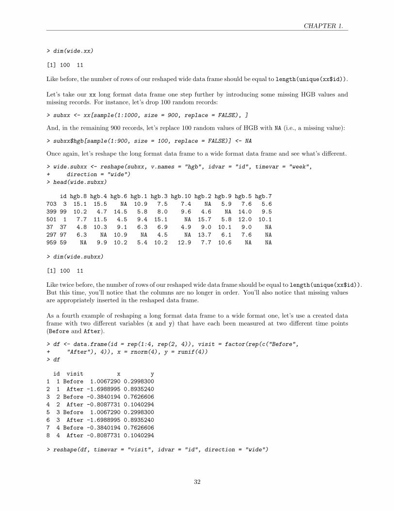
CHAPTER 1.
> dim(wide.xx)
[1] 100 11
Like before, the number of rows of our reshaped wide data frame should be equal to length(unique(xx$id)).
Let’s take our xx long format data frame one step further by introducing some missing HGB values andmissing records. For instance, let’s drop 100 random records:
> subxx <- xx[sample(1:1000, size = 900, replace = FALSE), ]
And, in the remaining 900 records, let’s replace 100 random values of HGB with NA (i.e., a missing value):
> subxx$hgb[sample(1:900, size = 100, replace = FALSE)] <- NA
Once again, let’s reshape the long format data frame to a wide format data frame and see what’s different.
> wide.subxx <- reshape(subxx, v.names = "hgb", idvar = "id", timevar = "week",
+ direction = "wide")
> head(wide.subxx)
id hgb.8 hgb.4 hgb.6 hgb.1 hgb.3 hgb.10 hgb.2 hgb.9 hgb.5 hgb.7703 3 15.1 15.5 NA 10.9 7.5 7.4 NA 5.9 7.6 5.6399 99 10.2 4.7 14.5 5.8 8.0 9.6 4.6 NA 14.0 9.5501 1 7.7 11.5 4.5 9.4 15.1 NA 15.7 5.8 12.0 10.137 37 4.8 10.3 9.1 6.3 6.9 4.9 9.0 10.1 9.0 NA297 97 6.3 NA 10.9 NA 4.5 NA 13.7 6.1 7.6 NA959 59 NA 9.9 10.2 5.4 10.2 12.9 7.7 10.6 NA NA
> dim(wide.subxx)
[1] 100 11
Like twice before, the number of rows of our reshaped wide data frame should be equal to length(unique(xx$id)).But this time, you’ll notice that the columns are no longer in order. You’ll also notice that missing valuesare appropriately inserted in the reshaped data frame.
As a fourth example of reshaping a long format data frame to a wide format one, let’s use a created dataframe with two different variables (x and y) that have each been measured at two different time points(Before and After).
> df <- data.frame(id = rep(1:4, rep(2, 4)), visit = factor(rep(c("Before",
+ "After"), 4)), x = rnorm(4), y = runif(4))
> df
id visit x y1 1 Before 1.0067290 0.29983002 1 After -1.6988995 0.89352403 2 Before -0.3840194 0.76266064 2 After -0.8087731 0.10402945 3 Before 1.0067290 0.29983006 3 After -1.6988995 0.89352407 4 Before -0.3840194 0.76266068 4 After -0.8087731 0.1040294
> reshape(df, timevar = "visit", idvar = "id", direction = "wide")
32
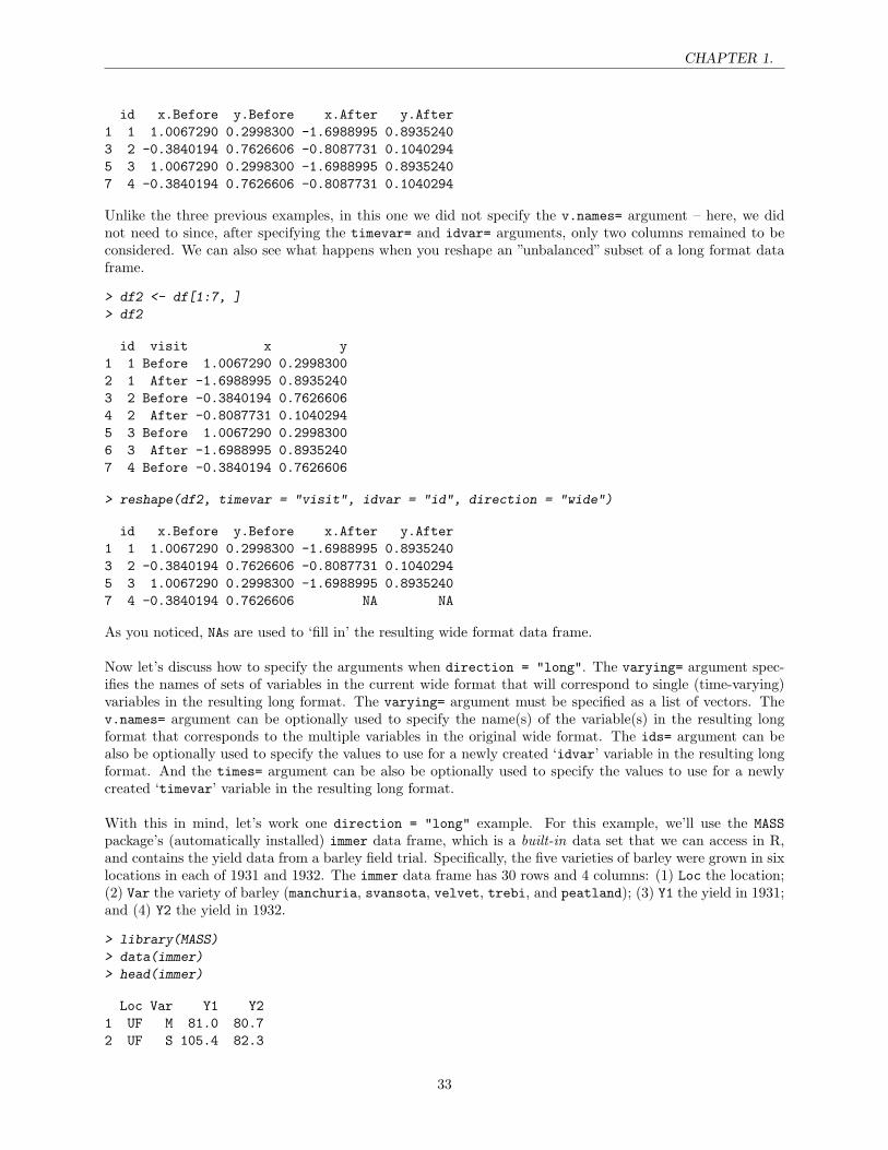
CHAPTER 1.
id x.Before y.Before x.After y.After1 1 1.0067290 0.2998300 -1.6988995 0.89352403 2 -0.3840194 0.7626606 -0.8087731 0.10402945 3 1.0067290 0.2998300 -1.6988995 0.89352407 4 -0.3840194 0.7626606 -0.8087731 0.1040294
Unlike the three previous examples, in this one we did not specify the v.names= argument – here, we didnot need to since, after specifying the timevar= and idvar= arguments, only two columns remained to beconsidered. We can also see what happens when you reshape an ”unbalanced” subset of a long format dataframe.
> df2 <- df[1:7, ]
> df2
id visit x y1 1 Before 1.0067290 0.29983002 1 After -1.6988995 0.89352403 2 Before -0.3840194 0.76266064 2 After -0.8087731 0.10402945 3 Before 1.0067290 0.29983006 3 After -1.6988995 0.89352407 4 Before -0.3840194 0.7626606
> reshape(df2, timevar = "visit", idvar = "id", direction = "wide")
id x.Before y.Before x.After y.After1 1 1.0067290 0.2998300 -1.6988995 0.89352403 2 -0.3840194 0.7626606 -0.8087731 0.10402945 3 1.0067290 0.2998300 -1.6988995 0.89352407 4 -0.3840194 0.7626606 NA NA
As you noticed, NAs are used to ‘fill in’ the resulting wide format data frame.
Now let’s discuss how to specify the arguments when direction = "long". The varying= argument spec-ifies the names of sets of variables in the current wide format that will correspond to single (time-varying)variables in the resulting long format. The varying= argument must be specified as a list of vectors. Thev.names= argument can be optionally used to specify the name(s) of the variable(s) in the resulting longformat that corresponds to the multiple variables in the original wide format. The ids= argument can bealso be optionally used to specify the values to use for a newly created ‘idvar’ variable in the resulting longformat. And the times= argument can be also be optionally used to specify the values to use for a newlycreated ‘timevar’ variable in the resulting long format.
With this in mind, let’s work one direction = "long" example. For this example, we’ll use the MASSpackage’s (automatically installed) immer data frame, which is a built-in data set that we can access in R,and contains the yield data from a barley field trial. Specifically, the five varieties of barley were grown in sixlocations in each of 1931 and 1932. The immer data frame has 30 rows and 4 columns: (1) Loc the location;(2) Var the variety of barley (manchuria, svansota, velvet, trebi, and peatland); (3) Y1 the yield in 1931;and (4) Y2 the yield in 1932.
> library(MASS)
> data(immer)
> head(immer)
Loc Var Y1 Y21 UF M 81.0 80.72 UF S 105.4 82.3
33
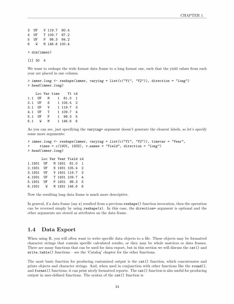
CHAPTER 1.
3 UF V 119.7 80.44 UF T 109.7 87.25 UF P 98.3 84.26 W M 146.6 100.4
> dim(immer)
[1] 30 4
We want to reshape the wide format data frame to a long format one, such that the yield values from eachyear are placed in one column.
> immer.long <- reshape(immer, varying = list(c("Y1", "Y2")), direction = "long")
> head(immer.long)
Loc Var time Y1 id1.1 UF M 1 81.0 12.1 UF S 1 105.4 23.1 UF V 1 119.7 34.1 UF T 1 109.7 45.1 UF P 1 98.3 56.1 W M 1 146.6 6
As you can see, just specifying the varying= argument doesn’t generate the clearest labels, so let’s specifysome more arguments:
> immer.long <- reshape(immer, varying = list(c("Y1", "Y2")), timevar = "Year",
+ times = c(1931, 1932), v.names = "Yield", direction = "long")
> head(immer.long)
Loc Var Year Yield id1.1931 UF M 1931 81.0 12.1931 UF S 1931 105.4 23.1931 UF V 1931 119.7 34.1931 UF T 1931 109.7 45.1931 UF P 1931 98.3 56.1931 W M 1931 146.6 6
Now the resulting long data frame is much more descriptive.
In general, if a data frame (say x) resulted from a previous reshape() function invocation, then the operationcan be reversed simply by using reshape(x). In this case, the direction= argument is optional and theother arguments are stored as attributes on the data frame.
1.4 Data Export
When using R, you will often want to write specific data objects to a file. These objects may be formattedcharacter strings that contain specific calculated results, or they may be whole matrices or data frames.There are many functions that can be used for data export, but in this section we will discuss the cat() andwrite.table() functions – see the ‘Catalog’ chapter for the other functions.
The most basic function for producing customized output is the cat() function, which concatenates andprints objects and character strings. And, when used in conjunction with other functions like the round(),and format() functions, it can print nicely formatted reports. The cat() function is also useful for producingoutput in user-defined functions. The syntax of the cat() function is
34
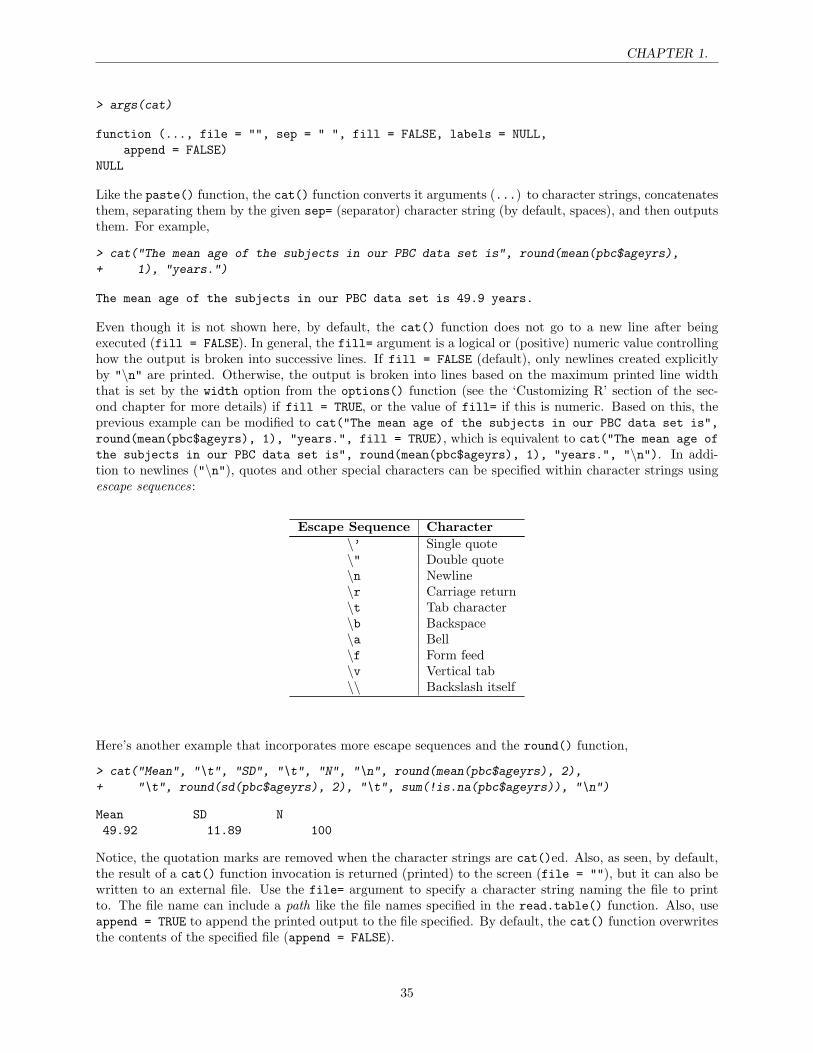
CHAPTER 1.
> args(cat)
function (..., file = "", sep = " ", fill = FALSE, labels = NULL,append = FALSE)
NULL
Like the paste() function, the cat() function converts it arguments (...) to character strings, concatenatesthem, separating them by the given sep= (separator) character string (by default, spaces), and then outputsthem. For example,
> cat("The mean age of the subjects in our PBC data set is", round(mean(pbc$ageyrs),
+ 1), "years.")
The mean age of the subjects in our PBC data set is 49.9 years.
Even though it is not shown here, by default, the cat() function does not go to a new line after beingexecuted (fill = FALSE). In general, the fill= argument is a logical or (positive) numeric value controllinghow the output is broken into successive lines. If fill = FALSE (default), only newlines created explicitlyby "\n" are printed. Otherwise, the output is broken into lines based on the maximum printed line widththat is set by the width option from the options() function (see the ‘Customizing R’ section of the sec-ond chapter for more details) if fill = TRUE, or the value of fill= if this is numeric. Based on this, theprevious example can be modified to cat("The mean age of the subjects in our PBC data set is",round(mean(pbc$ageyrs), 1), "years.", fill = TRUE), which is equivalent to cat("The mean age ofthe subjects in our PBC data set is", round(mean(pbc$ageyrs), 1), "years.", "\n"). In addi-tion to newlines ("\n"), quotes and other special characters can be specified within character strings usingescape sequences:
Escape Sequence Character\’ Single quote\" Double quote\n Newline\r Carriage return\t Tab character\b Backspace\a Bell\f Form feed\v Vertical tab\\ Backslash itself
Here’s another example that incorporates more escape sequences and the round() function,
> cat("Mean", "\t", "SD", "\t", "N", "\n", round(mean(pbc$ageyrs), 2),
+ "\t", round(sd(pbc$ageyrs), 2), "\t", sum(!is.na(pbc$ageyrs)), "\n")
Mean SD N49.92 11.89 100
Notice, the quotation marks are removed when the character strings are cat()ed. Also, as seen, by default,the result of a cat() function invocation is returned (printed) to the screen (file = ""), but it can also bewritten to an external file. Use the file= argument to specify a character string naming the file to printto. The file name can include a path like the file names specified in the read.table() function. Also, useappend = TRUE to append the printed output to the file specified. By default, the cat() function overwritesthe contents of the specified file (append = FALSE).
35
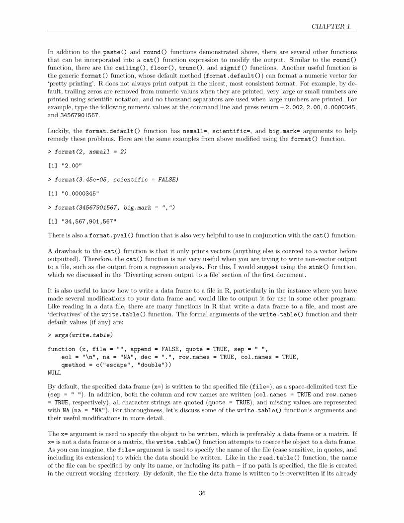
CHAPTER 1.
In addition to the paste() and round() functions demonstrated above, there are several other functionsthat can be incorporated into a cat() function expression to modify the output. Similar to the round()function, there are the ceiling(), floor(), trunc(), and signif() functions. Another useful function isthe generic format() function, whose default method (format.default()) can format a numeric vector for‘pretty printing’. R does not always print output in the nicest, most consistent format. For example, by de-fault, trailing zeros are removed from numeric values when they are printed, very large or small numbers areprinted using scientific notation, and no thousand separators are used when large numbers are printed. Forexample, type the following numeric values at the command line and press return – 2.002, 2.00, 0.0000345,and 34567901567.
Luckily, the format.default() function has nsmall=, scientific=, and big.mark= arguments to helpremedy these problems. Here are the same examples from above modified using the format() function.
> format(2, nsmall = 2)
[1] "2.00"
> format(3.45e-05, scientific = FALSE)
[1] "0.0000345"
> format(34567901567, big.mark = ",")
[1] "34,567,901,567"
There is also a format.pval() function that is also very helpful to use in conjunction with the cat() function.
A drawback to the cat() function is that it only prints vectors (anything else is coerced to a vector beforeoutputted). Therefore, the cat() function is not very useful when you are trying to write non-vector outputto a file, such as the output from a regression analysis. For this, I would suggest using the sink() function,which we discussed in the ‘Diverting screen output to a file’ section of the first document.
It is also useful to know how to write a data frame to a file in R, particularly in the instance where you havemade several modifications to your data frame and would like to output it for use in some other program.Like reading in a data file, there are many functions in R that write a data frame to a file, and most are‘derivatives’ of the write.table() function. The formal arguments of the write.table() function and theirdefault values (if any) are:
> args(write.table)
function (x, file = "", append = FALSE, quote = TRUE, sep = " ",eol = "\n", na = "NA", dec = ".", row.names = TRUE, col.names = TRUE,qmethod = c("escape", "double"))
NULL
By default, the specified data frame (x=) is written to the specified file (file=), as a space-delimited text file(sep = " "). In addition, both the column and row names are written (col.names = TRUE and row.names= TRUE, respectively), all character strings are quoted (quote = TRUE), and missing values are representedwith NA (na = "NA"). For thoroughness, let’s discuss some of the write.table() function’s arguments andtheir useful modifications in more detail.
The x= argument is used to specify the object to be written, which is preferably a data frame or a matrix. Ifx= is not a data frame or a matrix, the write.table() function attempts to coerce the object to a data frame.As you can imagine, the file= argument is used to specify the name of the file (case sensitive, in quotes, andincluding its extension) to which the data should be written. Like in the read.table() function, the nameof the file can be specified by only its name, or including its path – if no path is specified, the file is createdin the current working directory. By default, the file the data frame is written to is overwritten if its already
36
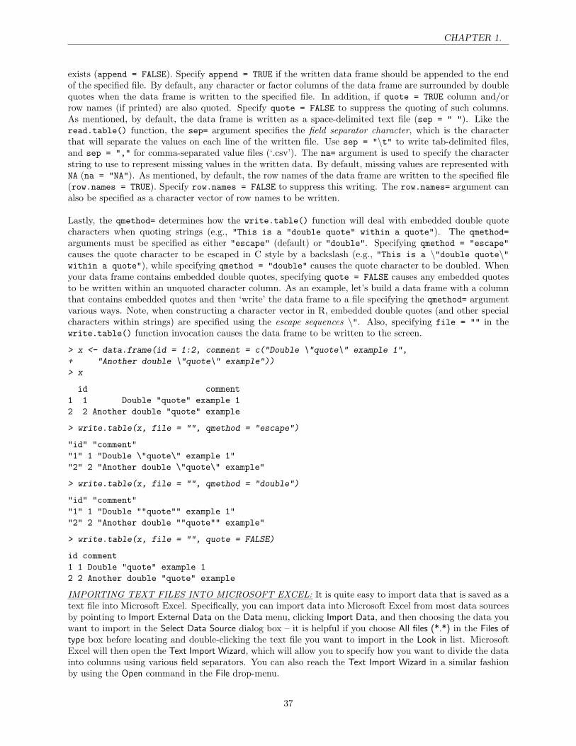
CHAPTER 1.
exists (append = FALSE). Specify append = TRUE if the written data frame should be appended to the endof the specified file. By default, any character or factor columns of the data frame are surrounded by doublequotes when the data frame is written to the specified file. In addition, if quote = TRUE column and/orrow names (if printed) are also quoted. Specify quote = FALSE to suppress the quoting of such columns.As mentioned, by default, the data frame is written as a space-delimited text file (sep = " "). Like theread.table() function, the sep= argument specifies the field separator character, which is the characterthat will separate the values on each line of the written file. Use sep = "\t" to write tab-delimited files,and sep = "," for comma-separated value files (‘.csv’). The na= argument is used to specify the characterstring to use to represent missing values in the written data. By default, missing values are represented withNA (na = "NA"). As mentioned, by default, the row names of the data frame are written to the specified file(row.names = TRUE). Specify row.names = FALSE to suppress this writing. The row.names= argument canalso be specified as a character vector of row names to be written.
Lastly, the qmethod= determines how the write.table() function will deal with embedded double quotecharacters when quoting strings (e.g., "This is a "double quote" within a quote"). The qmethod=arguments must be specified as either "escape" (default) or "double". Specifying qmethod = "escape"causes the quote character to be escaped in C style by a backslash (e.g., "This is a \"double quote\"within a quote"), while specifying qmethod = "double" causes the quote character to be doubled. Whenyour data frame contains embedded double quotes, specifying quote = FALSE causes any embedded quotesto be written within an unquoted character column. As an example, let’s build a data frame with a columnthat contains embedded quotes and then ‘write’ the data frame to a file specifying the qmethod= argumentvarious ways. Note, when constructing a character vector in R, embedded double quotes (and other specialcharacters within strings) are specified using the escape sequences \". Also, specifying file = "" in thewrite.table() function invocation causes the data frame to be written to the screen.
> x <- data.frame(id = 1:2, comment = c("Double \"quote\" example 1",
+ "Another double \"quote\" example"))
> x
id comment1 1 Double "quote" example 12 2 Another double "quote" example
> write.table(x, file = "", qmethod = "escape")
"id" "comment""1" 1 "Double \"quote\" example 1""2" 2 "Another double \"quote\" example"
> write.table(x, file = "", qmethod = "double")
"id" "comment""1" 1 "Double ""quote"" example 1""2" 2 "Another double ""quote"" example"
> write.table(x, file = "", quote = FALSE)
id comment1 1 Double "quote" example 12 2 Another double "quote" example
IMPORTING TEXT FILES INTO MICROSOFT EXCEL: It is quite easy to import data that is saved as atext file into Microsoft Excel. Specifically, you can import data into Microsoft Excel from most data sourcesby pointing to Import External Data on the Data menu, clicking Import Data, and then choosing the data youwant to import in the Select Data Source dialog box – it is helpful if you choose All files (*.*) in the Files oftype box before locating and double-clicking the text file you want to import in the Look in list. MicrosoftExcel will then open the Text Import Wizard, which will allow you to specify how you want to divide the datainto columns using various field separators. You can also reach the Text Import Wizard in a similar fashionby using the Open command in the File drop-menu.
37
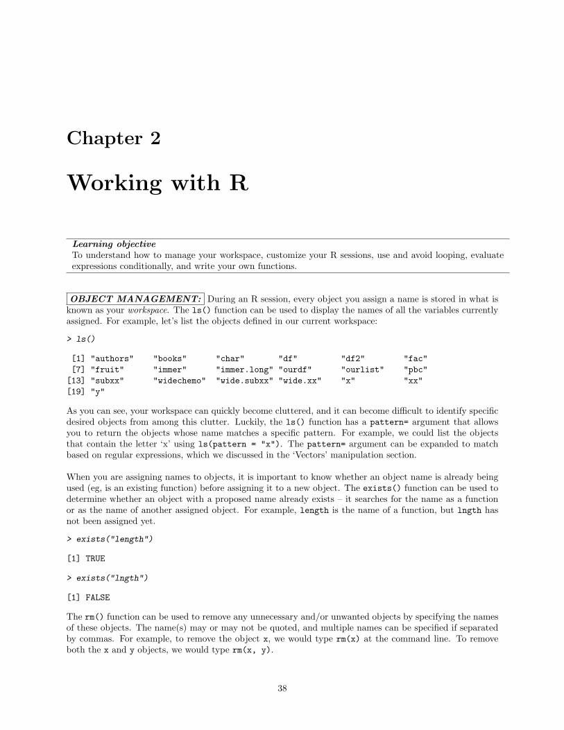
Chapter 2
Working with R
Learning objectiveTo understand how to manage your workspace, customize your R sessions, use and avoid looping, evaluateexpressions conditionally, and write your own functions.
OBJECT MANAGEMENT: During an R session, every object you assign a name is stored in what isknown as your workspace. The ls() function can be used to display the names of all the variables currentlyassigned. For example, let’s list the objects defined in our current workspace:
> ls()
[1] "authors" "books" "char" "df" "df2" "fac"[7] "fruit" "immer" "immer.long" "ourdf" "ourlist" "pbc"[13] "subxx" "widechemo" "wide.subxx" "wide.xx" "x" "xx"[19] "y"
As you can see, your workspace can quickly become cluttered, and it can become difficult to identify specificdesired objects from among this clutter. Luckily, the ls() function has a pattern= argument that allowsyou to return the objects whose name matches a specific pattern. For example, we could list the objectsthat contain the letter ‘x’ using ls(pattern = "x"). The pattern= argument can be expanded to matchbased on regular expressions, which we discussed in the ‘Vectors’ manipulation section.
When you are assigning names to objects, it is important to know whether an object name is already beingused (eg, is an existing function) before assigning it to a new object. The exists() function can be used todetermine whether an object with a proposed name already exists – it searches for the name as a functionor as the name of another assigned object. For example, length is the name of a function, but lngth hasnot been assigned yet.
> exists("length")
[1] TRUE
> exists("lngth")
[1] FALSE
The rm() function can be used to remove any unnecessary and/or unwanted objects by specifying the namesof these objects. The name(s) may or may not be quoted, and multiple names can be specified if separatedby commas. For example, to remove the object x, we would type rm(x) at the command line. To removeboth the x and y objects, we would type rm(x, y).
38

CHAPTER 2. WORKING WITH R
Multiple names can also be given in a vector form as a quoted string to the list= argument. Therefore,the previous example could be typed as: rm(list=c("x", "y")). We can use this list= argument in con-junction with the ls() function to easily remove all of the objects in your workspace by typing rm(list =ls()). In the Windows version of R, the entire current workspace can also be cleared by selecting Removeall objects from the Misc drop-menu. We can also take this example one step further by incorporating thesetdiff() function, which returns the difference between two sets of elements, to remove all objects exceptspecified ones from your current workspace: rm(list = setdiff(ls(), c(object1, object2))), whereobject1 and object2 are those objects you wish to keep.
→ Practice Exercise: Let’s remove all the defined objects in our workspace except our pbc data frame.
> rm(list = setdiff(ls(), "pbc"))
> ls()
[1] "pbc"
There are also several ways to save desired objects. Recall, when you quit R, you are asked Save yourworkspace image? Accepting this offer will save all the objects in your current workspace to a directoryspecific hidden file named .RData1. If you saved your workspace before quitting and start R from the samedirectory at a later time, R loads this saved workspace and all of the objects are restored to the currentworkspace. However, I would highly recommend cleaning up your workspace using the rm() function beforesaving your workspace. The save.image() function can also be explicitly used to save the current workspace.By default, the objects are saved to the .RData hidden file, but a different file name can be specified usingthe file= argument. Unfortunately both of these methods are very inefficient and use a lot of memory tosave the workspace.
An alternative is to use the save() function, which allows you to save specific objects and has an op-tion to compress the file the objects are saved to. This is extremely useful when dealing with largeobjects that take significant execution time to create and/or normally take up scarce memory. Specifycompress = TRUE to store the specified file very compactly – save(list = c("object1", "object2"),file = "objects.rda", compress = TRUE), where object1 and object2 are those objects you wish tosave, and objects.rda is the file you wish to compactly save them too. You then use load("objects.rda")to reload the saved objects at a later time (i.e., in another R session).
CUSTOMIZING R SESSIONS: The (possible) loading of objects from a saved image of the previousworkspace from the hidden .RData file (if the workspace was saved) is just one step in the ‘startup’ procedurethat R goes through when an R session is started. This startup procedure also sources (1) environment files,which contain lists of environment variables to be set, and (2) profile files, which contain R code used toload specific packages, to define important functions, and to define specific environment options, which affectthe way in which R computes and displays its results. The nice thing is that we can modify the profile filessourced in this procedure in order to customize our R sessions. However, even though we can access theenvironment files, it is not recommended to modify these files.
After searching for and sourcing the environment files, R first searches for and sources a ‘site-wide’ startupprofile file named Rprofile.site, which is located in the R_HOME/etc directory (if it exists). Recall, ona Linux, Unix, or Mac machine, R_HOME is /usr/lib/R or /usr/local/lib/R. On a Windows machineR_HOME is C:\Program Files\R\R-version, where version is the R version number (e.g., 2.5.1). TheRprofile.site file is termed ‘site-wide’ because this file is sourced every time R is started, no matter whatdirectory R is started in – so think of it as a ‘global’ file. In turn, the Rprofile.site files contains the ex-pressions that you want to execute every time R is started anywhere on your machine. A second, ‘personal’,hidden file named .Rprofile can also be placed in any directory. In turn, R will source a hidden .Rprofilefile if R is started in a directory that contains such a file. In contrast to the global Rprofile.site file, but
1By default, hidden files like .RData will not appear in a folder/directory. On a Unix/Linux machine, use ls -a at theshell command prompt to list all files, including hidden files. On a Windows machine, select Folder Options. . . from the Viewdrop-menu. Then select Show all files from the View tab of the Folder Options dialog box.
39
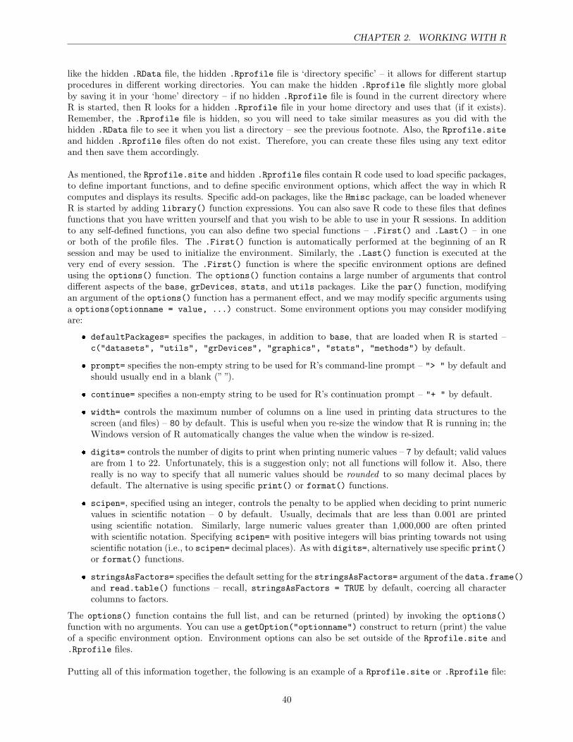
CHAPTER 2. WORKING WITH R
like the hidden .RData file, the hidden .Rprofile file is ‘directory specific’ – it allows for different startupprocedures in different working directories. You can make the hidden .Rprofile file slightly more globalby saving it in your ‘home’ directory – if no hidden .Rprofile file is found in the current directory whereR is started, then R looks for a hidden .Rprofile file in your home directory and uses that (if it exists).Remember, the .Rprofile file is hidden, so you will need to take similar measures as you did with thehidden .RData file to see it when you list a directory – see the previous footnote. Also, the Rprofile.siteand hidden .Rprofile files often do not exist. Therefore, you can create these files using any text editorand then save them accordingly.
As mentioned, the Rprofile.site and hidden .Rprofile files contain R code used to load specific packages,to define important functions, and to define specific environment options, which affect the way in which Rcomputes and displays its results. Specific add-on packages, like the Hmisc package, can be loaded wheneverR is started by adding library() function expressions. You can also save R code to these files that definesfunctions that you have written yourself and that you wish to be able to use in your R sessions. In additionto any self-defined functions, you can also define two special functions – .First() and .Last() – in oneor both of the profile files. The .First() function is automatically performed at the beginning of an Rsession and may be used to initialize the environment. Similarly, the .Last() function is executed at thevery end of every session. The .First() function is where the specific environment options are definedusing the options() function. The options() function contains a large number of arguments that controldifferent aspects of the base, grDevices, stats, and utils packages. Like the par() function, modifyingan argument of the options() function has a permanent effect, and we may modify specific arguments usinga options(optionname = value, ...) construct. Some environment options you may consider modifyingare:
defaultPackages= specifies the packages, in addition to base, that are loaded when R is started –c("datasets", "utils", "grDevices", "graphics", "stats", "methods") by default.
prompt= specifies the non-empty string to be used for R’s command-line prompt – "> " by default andshould usually end in a blank (” ”).
continue= specifies a non-empty string to be used for R’s continuation prompt – "+ " by default.
width= controls the maximum number of columns on a line used in printing data structures to thescreen (and files) – 80 by default. This is useful when you re-size the window that R is running in; theWindows version of R automatically changes the value when the window is re-sized.
digits= controls the number of digits to print when printing numeric values – 7 by default; valid valuesare from 1 to 22. Unfortunately, this is a suggestion only; not all functions will follow it. Also, therereally is no way to specify that all numeric values should be rounded to so many decimal places bydefault. The alternative is using specific print() or format() functions.
scipen=, specified using an integer, controls the penalty to be applied when deciding to print numericvalues in scientific notation – 0 by default. Usually, decimals that are less than 0.001 are printedusing scientific notation. Similarly, large numeric values greater than 1,000,000 are often printedwith scientific notation. Specifying scipen= with positive integers will bias printing towards not usingscientific notation (i.e., to scipen= decimal places). As with digits=, alternatively use specific print()or format() functions.
stringsAsFactors= specifies the default setting for the stringsAsFactors= argument of the data.frame()and read.table() functions – recall, stringsAsFactors = TRUE by default, coercing all charactercolumns to factors.
The options() function contains the full list, and can be returned (printed) by invoking the options()function with no arguments. You can use a getOption("optionname") construct to return (print) the valueof a specific environment option. Environment options can also be set outside of the Rprofile.site and.Rprofile files.
Putting all of this information together, the following is an example of a Rprofile.site or .Rprofile file:
40

CHAPTER 2. WORKING WITH R
# Load the Hmisc packagelibrary(Hmisc)
# Modify the command line and continuation prompt, and the widthoptions(prompt="$ ", continue="+\t", width = 100)
# Source a file that contains several self-defined functionssource(file.path(Sys.getenv("HOME"), "R", "mystuff.R"))
# Modify the q() function to automatically quit _without_ saving the workspace# (and without prompting)q <- function(save = "no", status = 0, runLast = TRUE)
.Internal(quit(save, status, runLast))
.Last <- function() # close all graphics window and file devices; a small safety measuregraphics.off()
In the Windows version of R, you can also customize the way the R console ‘looks and feels’ using the GUIpreferences selection under the Edit drop-menu.
CONDITIONAL EVALUATION: Up to this point, we have evaluated single expressions or multipleexpressions grouped with the curly braces, . However, we will often want to conditionally evaluates oneor several expression. For example, perhaps we wish to calculate the mean of a continuous vector if thevalues are normally distributed, or the median if they are not. Conditional evaluation will also come inhandy when you want to generalize your R code and perhaps incorporate it into a self-defined function. InR, an if statement allows us to evaluate expressions based on a condition, and takes one of two forms. Thefirst is the ‘if-then’ form:
if(condition) expression(s) if condition is TRUE
The condition is an expression that, when evaluated, returns a single TRUE or FALSE value – an error isreturned if the condition does not evaluate to a logical value. If the condition evaluates to TRUE, then anyexpression(s) between the braces ( and ) is/are evaluated. The second form is an ‘if-then-else’ form:
if(condition) expression(s) if condition is TRUE
else expression(s) if condition is FALSE
In this form, the condition is evaluated, and any expression(s) between the first set of curly braces is/areevaluated if the condition evaluates to TRUE. If the condition evaluates to FALSE, then the expression(s)between the second set of curly braces is/are evaluated. The ‘if-then-else’ form of the if statement can alsobe nested.
if(condition1) expression(s) if condition1 is TRUE
else if(condition2) expression(s) if condition 1 is FALSE but condition2 is TRUE
else if(condition3) expression(s) if both condition1 and 2 are FALSE but condition3 is TRUE
41
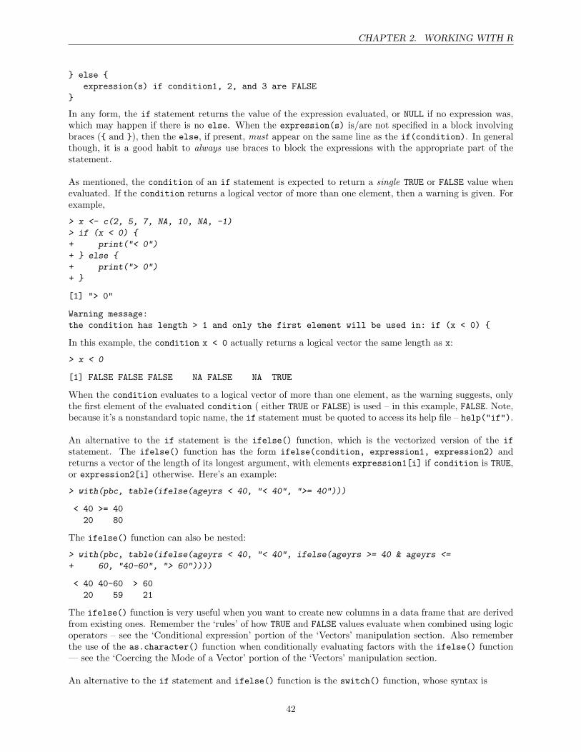
CHAPTER 2. WORKING WITH R
else expression(s) if condition1, 2, and 3 are FALSE
In any form, the if statement returns the value of the expression evaluated, or NULL if no expression was,which may happen if there is no else. When the expression(s) is/are not specified in a block involvingbraces ( and ), then the else, if present, must appear on the same line as the if(condition). In generalthough, it is a good habit to always use braces to block the expressions with the appropriate part of thestatement.
As mentioned, the condition of an if statement is expected to return a single TRUE or FALSE value whenevaluated. If the condition returns a logical vector of more than one element, then a warning is given. Forexample,
> x <- c(2, 5, 7, NA, 10, NA, -1)
> if (x < 0)
+ print("< 0")
+ else
+ print("> 0")
+
[1] "> 0"
Warning message:the condition has length > 1 and only the first element will be used in: if (x < 0)
In this example, the condition x < 0 actually returns a logical vector the same length as x:
> x < 0
[1] FALSE FALSE FALSE NA FALSE NA TRUE
When the condition evaluates to a logical vector of more than one element, as the warning suggests, onlythe first element of the evaluated condition ( either TRUE or FALSE) is used – in this example, FALSE. Note,because it’s a nonstandard topic name, the if statement must be quoted to access its help file – help("if").
An alternative to the if statement is the ifelse() function, which is the vectorized version of the ifstatement. The ifelse() function has the form ifelse(condition, expression1, expression2) andreturns a vector of the length of its longest argument, with elements expression1[i] if condition is TRUE,or expression2[i] otherwise. Here’s an example:
> with(pbc, table(ifelse(ageyrs < 40, "< 40", ">= 40")))
< 40 >= 4020 80
The ifelse() function can also be nested:
> with(pbc, table(ifelse(ageyrs < 40, "< 40", ifelse(ageyrs >= 40 & ageyrs <=
+ 60, "40-60", "> 60"))))
< 40 40-60 > 6020 59 21
The ifelse() function is very useful when you want to create new columns in a data frame that are derivedfrom existing ones. Remember the ‘rules’ of how TRUE and FALSE values evaluate when combined using logicoperators – see the ‘Conditional expression’ portion of the ‘Vectors’ manipulation section. Also rememberthe use of the as.character() function when conditionally evaluating factors with the ifelse() function— see the ‘Coercing the Mode of a Vector’ portion of the ‘Vectors’ manipulation section.
An alternative to the if statement and ifelse() function is the switch() function, whose syntax is
42
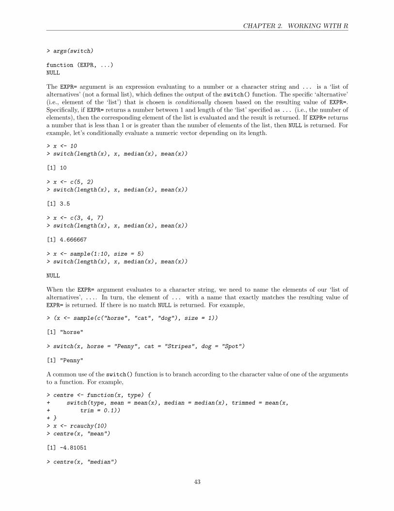
CHAPTER 2. WORKING WITH R
> args(switch)
function (EXPR, ...)NULL
The EXPR= argument is an expression evaluating to a number or a character string and ... is a ‘list ofalternatives’ (not a formal list), which defines the output of the switch() function. The specific ‘alternative’(i.e., element of the ‘list’) that is chosen is conditionally chosen based on the resulting value of EXPR=.Specifically, if EXPR= returns a number between 1 and length of the ‘list’ specified as ... (i.e., the number ofelements), then the corresponding element of the list is evaluated and the result is returned. If EXPR= returnsa number that is less than 1 or is greater than the number of elements of the list, then NULL is returned. Forexample, let’s conditionally evaluate a numeric vector depending on its length.
> x <- 10
> switch(length(x), x, median(x), mean(x))
[1] 10
> x <- c(5, 2)
> switch(length(x), x, median(x), mean(x))
[1] 3.5
> x <- c(3, 4, 7)
> switch(length(x), x, median(x), mean(x))
[1] 4.666667
> x <- sample(1:10, size = 5)
> switch(length(x), x, median(x), mean(x))
NULL
When the EXPR= argument evaluates to a character string, we need to name the elements of our ‘list ofalternatives’, .... In turn, the element of ... with a name that exactly matches the resulting value ofEXPR= is returned. If there is no match NULL is returned. For example,
> (x <- sample(c("horse", "cat", "dog"), size = 1))
[1] "horse"
> switch(x, horse = "Penny", cat = "Stripes", dog = "Spot")
[1] "Penny"
A common use of the switch() function is to branch according to the character value of one of the argumentsto a function. For example,
> centre <- function(x, type)
+ switch(type, mean = mean(x), median = median(x), trimmed = mean(x,
+ trim = 0.1))
+
> x <- rcauchy(10)
> centre(x, "mean")
[1] -4.81051
> centre(x, "median")
43
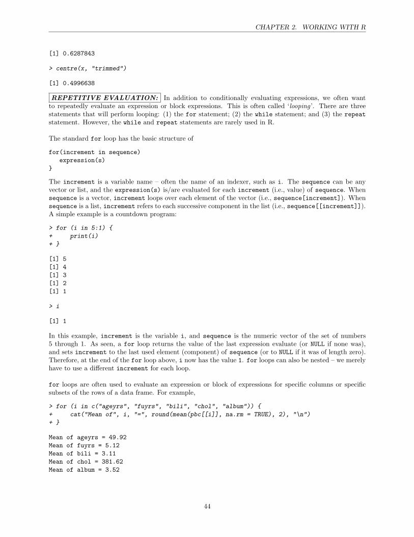
CHAPTER 2. WORKING WITH R
[1] 0.6287843
> centre(x, "trimmed")
[1] 0.4996638
REPETITIVE EVALUATION: In addition to conditionally evaluating expressions, we often wantto repeatedly evaluate an expression or block expressions. This is often called ‘looping ’. There are threestatements that will perform looping: (1) the for statement; (2) the while statement; and (3) the repeatstatement. However, the while and repeat statements are rarely used in R.
The standard for loop has the basic structure of
for(increment in sequence)expression(s)
The increment is a variable name – often the name of an indexer, such as i. The sequence can be anyvector or list, and the expression(s) is/are evaluated for each increment (i.e., value) of sequence. Whensequence is a vector, increment loops over each element of the vector (i.e., sequence[increment]). Whensequence is a list, increment refers to each successive component in the list (i.e., sequence[[increment]]).A simple example is a countdown program:
> for (i in 5:1)
+ print(i)
+
[1] 5[1] 4[1] 3[1] 2[1] 1
> i
[1] 1
In this example, increment is the variable i, and sequence is the numeric vector of the set of numbers5 through 1. As seen, a for loop returns the value of the last expression evaluate (or NULL if none was),and sets increment to the last used element (component) of sequence (or to NULL if it was of length zero).Therefore, at the end of the for loop above, i now has the value 1. for loops can also be nested – we merelyhave to use a different increment for each loop.
for loops are often used to evaluate an expression or block of expressions for specific columns or specificsubsets of the rows of a data frame. For example,
> for (i in c("ageyrs", "fuyrs", "bili", "chol", "album"))
+ cat("Mean of", i, "=", round(mean(pbc[[i]], na.rm = TRUE), 2), "\n")
+
Mean of ageyrs = 49.92Mean of fuyrs = 5.12Mean of bili = 3.11Mean of chol = 381.62Mean of album = 3.52
44

CHAPTER 2. WORKING WITH R
> for (i in c("ageyrs", "fuyrs", "bili", "chol", "album"))
+ for (j in levels(pbc$sex))
+ cat("Mean of", i, "in", j, "patients =", round(mean(pbc[pbc$sex ==
+ j & !is.na(pbc$sex), i], na.rm = TRUE), 2), "\n")
+
+
Mean of ageyrs in Female patients = 49.07Mean of ageyrs in Male patients = 55.16Mean of fuyrs in Female patients = 5.13Mean of fuyrs in Male patients = 5.04Mean of bili in Female patients = 3Mean of bili in Male patients = 3.79Mean of chol in Female patients = 374.74Mean of chol in Male patients = 417.27Mean of album in Female patients = 3.5Mean of album in Male patients = 3.63
In these examples we incremented across the elements of a character vector and took advantage of the doublesquare brackets, [[ ]], and [ , ] subsetting constructs to extract the rows and columns of our pbc dataframe. As you can imagine, the dfname$colname construct does not work well with for loops.
IMPORTANT: Using a for loop is not always necessary in R. As we have already seen, many functionsand operators are vectorized. In the ‘Family of apply() functions’ section , we will also encounter additionalfunctions that perform implicit looping. In general, avoiding loops can make your R code more compact,easier to read, and often times more efficient in execution.
Let’s get back to repetitive evaluation. . . Obviously, the for loop is great to use when you know ahead oftime what sequence of values you want to loop over. However, sometimes you don’t know this. In this case,you may want to repeat something as long as a condition is met (e.g., as long as a number is positive, or anumber is larger than some tolerance). For this, use a while loop:
while(condition) expression(s)
Like the if statement, the condition is an expression that, when evaluated, returns a single TRUE or FALSEvalue. If the condition evaluates to TRUE, then any expression(s) between the curly braces ( and )is/are evaluated. This process continues until the condition evaluates to FALSE. Like the for loop, thewhile loop returns the value of the last evaluation of the expression(s). For example,
> i <- 1
> while (i <= 5)
+ cat("Iteration", i, "\n")
+ i <- i + 1
+
Iteration 1Iteration 2Iteration 3Iteration 4Iteration 5
> i
[1] 6
45
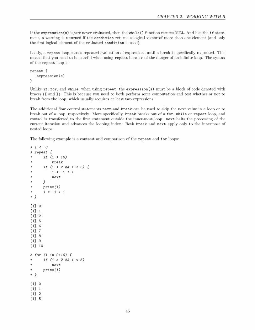
CHAPTER 2. WORKING WITH R
If the expression(s) is/are never evaluated, then the while() function returns NULL. And like the if state-ment, a warning is returned if the condition returns a logical vector of more than one element (and onlythe first logical element of the evaluated condition is used).
Lastly, a repeat loop causes repeated evaluation of expressions until a break is specifically requested. Thismeans that you need to be careful when using repeat because of the danger of an infinite loop. The syntaxof the repeat loop is
repeat expression(s)
Unlike if, for, and while, when using repeat, the expression(s) must be a block of code denoted withbraces ( and ). This is because you need to both perform some computation and test whether or not tobreak from the loop, which usually requires at least two expressions.
The additional flow control statements next and break can be used to skip the next value in a loop or tobreak out of a loop, respectively. More specifically, break breaks out of a for, while or repeat loop, andcontrol is transferred to the first statement outside the inner-most loop. next halts the processing of thecurrent iteration and advances the looping index. Both break and next apply only to the innermost ofnested loops.
The following example is a contrast and comparison of the repeat and for loops:
> i <- 0
> repeat
+ if (i > 10)
+ break
+ if (i > 2 && i < 5)
+ i <- i + 1
+ next
+
+ print(i)
+ i <- i + 1
+
[1] 0[1] 1[1] 2[1] 5[1] 6[1] 7[1] 8[1] 9[1] 10
> for (i in 0:10)
+ if (i > 2 && i < 5)
+ next
+ print(i)
+
[1] 0[1] 1[1] 2[1] 5
46
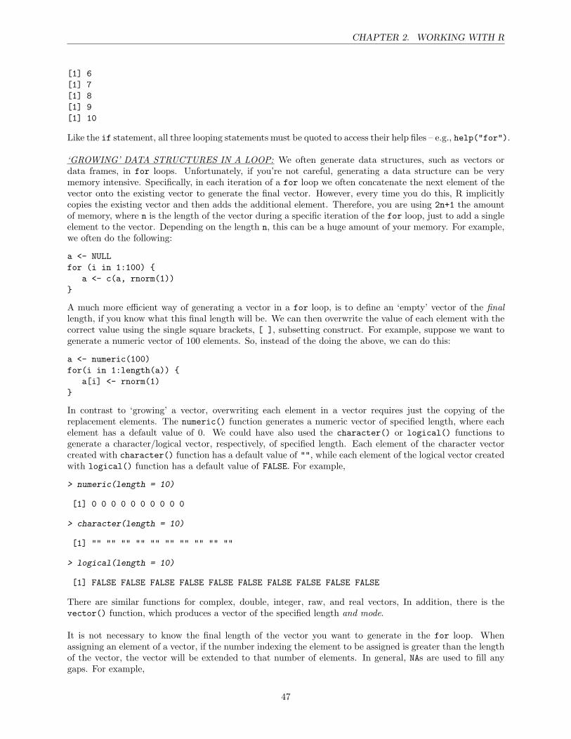
CHAPTER 2. WORKING WITH R
[1] 6[1] 7[1] 8[1] 9[1] 10
Like the if statement, all three looping statements must be quoted to access their help files – e.g., help("for").
‘GROWING’ DATA STRUCTURES IN A LOOP: We often generate data structures, such as vectors ordata frames, in for loops. Unfortunately, if you’re not careful, generating a data structure can be verymemory intensive. Specifically, in each iteration of a for loop we often concatenate the next element of thevector onto the existing vector to generate the final vector. However, every time you do this, R implicitlycopies the existing vector and then adds the additional element. Therefore, you are using 2n+1 the amountof memory, where n is the length of the vector during a specific iteration of the for loop, just to add a singleelement to the vector. Depending on the length n, this can be a huge amount of your memory. For example,we often do the following:
a <- NULLfor (i in 1:100)
a <- c(a, rnorm(1))
A much more efficient way of generating a vector in a for loop, is to define an ‘empty’ vector of the finallength, if you know what this final length will be. We can then overwrite the value of each element with thecorrect value using the single square brackets, [ ], subsetting construct. For example, suppose we want togenerate a numeric vector of 100 elements. So, instead of the doing the above, we can do this:
a <- numeric(100)for(i in 1:length(a))
a[i] <- rnorm(1)
In contrast to ‘growing’ a vector, overwriting each element in a vector requires just the copying of thereplacement elements. The numeric() function generates a numeric vector of specified length, where eachelement has a default value of 0. We could have also used the character() or logical() functions togenerate a character/logical vector, respectively, of specified length. Each element of the character vectorcreated with character() function has a default value of "", while each element of the logical vector createdwith logical() function has a default value of FALSE. For example,
> numeric(length = 10)
[1] 0 0 0 0 0 0 0 0 0 0
> character(length = 10)
[1] "" "" "" "" "" "" "" "" "" ""
> logical(length = 10)
[1] FALSE FALSE FALSE FALSE FALSE FALSE FALSE FALSE FALSE FALSE
There are similar functions for complex, double, integer, raw, and real vectors, In addition, there is thevector() function, which produces a vector of the specified length and mode.
It is not necessary to know the final length of the vector you want to generate in the for loop. Whenassigning an element of a vector, if the number indexing the element to be assigned is greater than the lengthof the vector, the vector will be extended to that number of elements. In general, NAs are used to fill anygaps. For example,
47
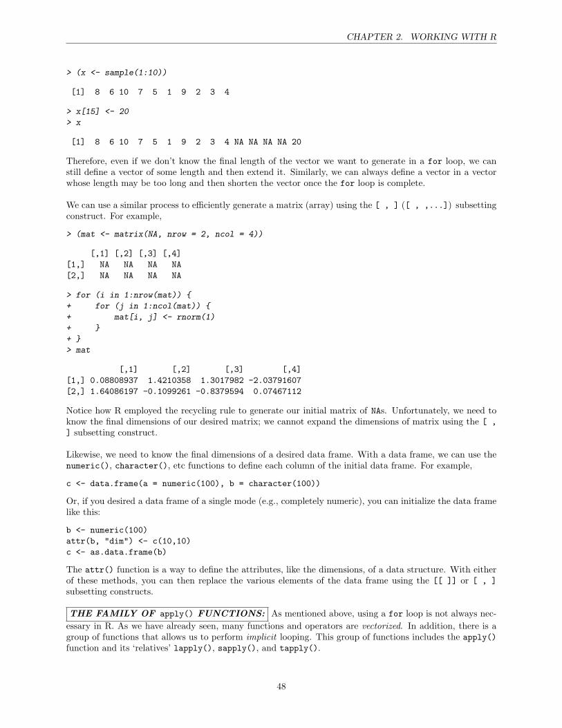
CHAPTER 2. WORKING WITH R
> (x <- sample(1:10))
[1] 8 6 10 7 5 1 9 2 3 4
> x[15] <- 20
> x
[1] 8 6 10 7 5 1 9 2 3 4 NA NA NA NA 20
Therefore, even if we don’t know the final length of the vector we want to generate in a for loop, we canstill define a vector of some length and then extend it. Similarly, we can always define a vector in a vectorwhose length may be too long and then shorten the vector once the for loop is complete.
We can use a similar process to efficiently generate a matrix (array) using the [ , ] ([ , ,...]) subsettingconstruct. For example,
> (mat <- matrix(NA, nrow = 2, ncol = 4))
[,1] [,2] [,3] [,4][1,] NA NA NA NA[2,] NA NA NA NA
> for (i in 1:nrow(mat))
+ for (j in 1:ncol(mat))
+ mat[i, j] <- rnorm(1)
+
+
> mat
[,1] [,2] [,3] [,4][1,] 0.08808937 1.4210358 1.3017982 -2.03791607[2,] 1.64086197 -0.1099261 -0.8379594 0.07467112
Notice how R employed the recycling rule to generate our initial matrix of NAs. Unfortunately, we need toknow the final dimensions of our desired matrix; we cannot expand the dimensions of matrix using the [ ,] subsetting construct.
Likewise, we need to know the final dimensions of a desired data frame. With a data frame, we can use thenumeric(), character(), etc functions to define each column of the initial data frame. For example,
c <- data.frame(a = numeric(100), b = character(100))
Or, if you desired a data frame of a single mode (e.g., completely numeric), you can initialize the data framelike this:
b <- numeric(100)attr(b, "dim") <- c(10,10)c <- as.data.frame(b)
The attr() function is a way to define the attributes, like the dimensions, of a data structure. With eitherof these methods, you can then replace the various elements of the data frame using the [[ ]] or [ , ]subsetting constructs.
THE FAMILY OF apply() FUNCTIONS: As mentioned above, using a for loop is not always nec-essary in R. As we have already seen, many functions and operators are vectorized. In addition, there is agroup of functions that allows us to perform implicit looping. This group of functions includes the apply()function and its ‘relatives’ lapply(), sapply(), and tapply().
48
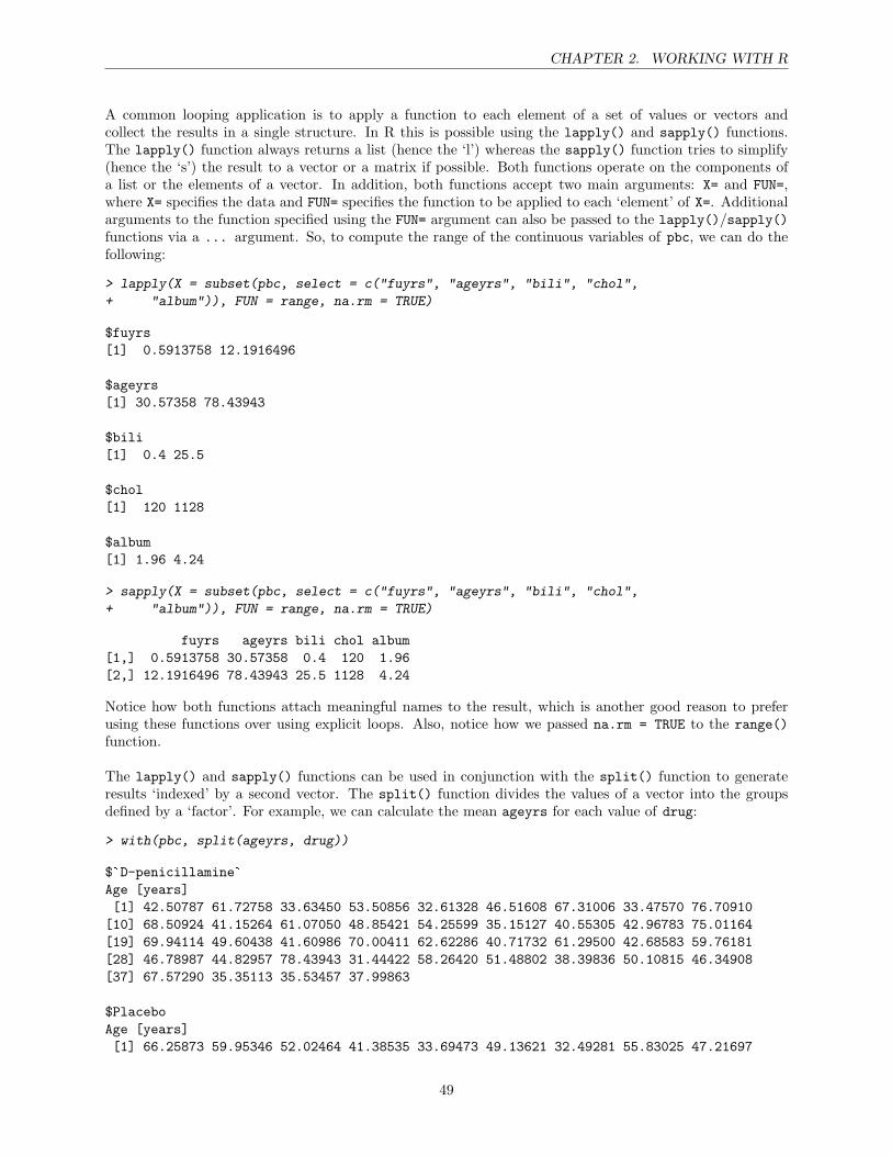
CHAPTER 2. WORKING WITH R
A common looping application is to apply a function to each element of a set of values or vectors andcollect the results in a single structure. In R this is possible using the lapply() and sapply() functions.The lapply() function always returns a list (hence the ‘l’) whereas the sapply() function tries to simplify(hence the ‘s’) the result to a vector or a matrix if possible. Both functions operate on the components ofa list or the elements of a vector. In addition, both functions accept two main arguments: X= and FUN=,where X= specifies the data and FUN= specifies the function to be applied to each ‘element’ of X=. Additionalarguments to the function specified using the FUN= argument can also be passed to the lapply()/sapply()functions via a ... argument. So, to compute the range of the continuous variables of pbc, we can do thefollowing:
> lapply(X = subset(pbc, select = c("fuyrs", "ageyrs", "bili", "chol",
+ "album")), FUN = range, na.rm = TRUE)
$fuyrs[1] 0.5913758 12.1916496
$ageyrs[1] 30.57358 78.43943
$bili[1] 0.4 25.5
$chol[1] 120 1128
$album[1] 1.96 4.24
> sapply(X = subset(pbc, select = c("fuyrs", "ageyrs", "bili", "chol",
+ "album")), FUN = range, na.rm = TRUE)
fuyrs ageyrs bili chol album[1,] 0.5913758 30.57358 0.4 120 1.96[2,] 12.1916496 78.43943 25.5 1128 4.24
Notice how both functions attach meaningful names to the result, which is another good reason to preferusing these functions over using explicit loops. Also, notice how we passed na.rm = TRUE to the range()function.
The lapply() and sapply() functions can be used in conjunction with the split() function to generateresults ‘indexed’ by a second vector. The split() function divides the values of a vector into the groupsdefined by a ‘factor’. For example, we can calculate the mean ageyrs for each value of drug:
> with(pbc, split(ageyrs, drug))
$`D-penicillamine`Age [years][1] 42.50787 61.72758 33.63450 53.50856 32.61328 46.51608 67.31006 33.47570 76.70910[10] 68.50924 41.15264 61.07050 48.85421 54.25599 35.15127 40.55305 42.96783 75.01164[19] 69.94114 49.60438 41.60986 70.00411 62.62286 40.71732 61.29500 42.68583 59.76181[28] 46.78987 44.82957 78.43943 31.44422 58.26420 51.48802 38.39836 50.10815 46.34908[37] 67.57290 35.35113 35.53457 37.99863
$PlaceboAge [years][1] 66.25873 59.95346 52.02464 41.38535 33.69473 49.13621 32.49281 55.83025 47.21697
49
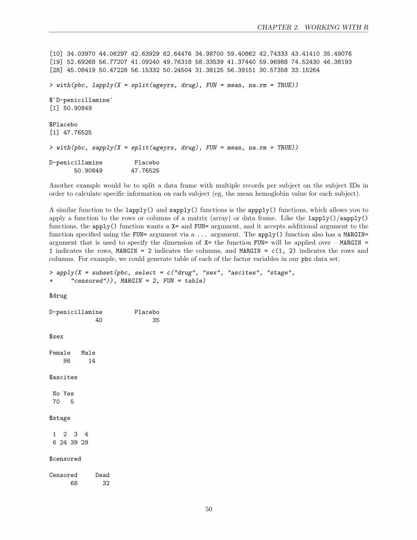
CHAPTER 2. WORKING WITH R
[10] 34.03970 44.06297 42.63929 62.64476 34.98700 59.40862 42.74333 43.41410 35.49076[19] 52.69268 56.77207 41.09240 49.76318 58.33539 41.37440 59.96988 74.52430 46.38193[28] 45.08419 50.47228 56.15332 50.24504 31.38125 56.39151 30.57358 33.15264
> with(pbc, lapply(X = split(ageyrs, drug), FUN = mean, na.rm = TRUE))
$`D-penicillamine`[1] 50.90849
$Placebo[1] 47.76525
> with(pbc, sapply(X = split(ageyrs, drug), FUN = mean, na.rm = TRUE))
D-penicillamine Placebo50.90849 47.76525
Another example would be to split a data frame with multiple records per subject on the subject IDs inorder to calculate specific information on each subject (eg, the mean hemoglobin value for each subject).
A similar function to the lapply() and sapply() functions is the appply() functions, which allows you toapply a function to the rows or columns of a matrix (array) or data frame. Like the lapply()/sapply()functions, the apply() function wants a X= and FUN= argument, and it accepts additional argument to thefunction specified using the FUN= argument via a ... argument. The apply() function also has a MARGIN=argument that is used to specify the dimension of X= the function FUN= will be applied over – MARGIN =1 indicates the rows, MARGIN = 2 indicates the columns, and MARGIN = c(1, 2) indicates the rows andcolumns. For example, we could generate table of each of the factor variables in our pbc data set:
> apply(X = subset(pbc, select = c("drug", "sex", "ascites", "stage",
+ "censored")), MARGIN = 2, FUN = table)
$drug
D-penicillamine Placebo40 35
$sex
Female Male86 14
$ascites
No Yes70 5
$stage
1 2 3 46 24 39 29
$censored
Censored Dead68 32
50
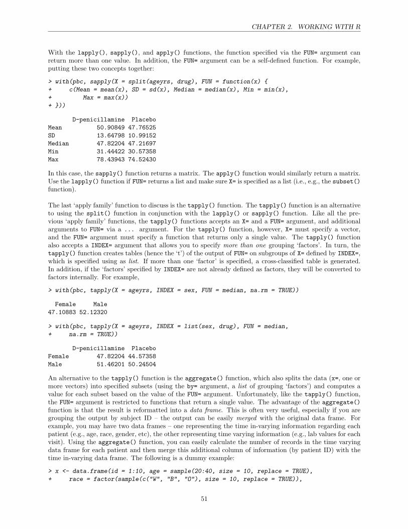
CHAPTER 2. WORKING WITH R
With the lapply(), sapply(), and apply() functions, the function specified via the FUN= argument canreturn more than one value. In addition, the FUN= argument can be a self-defined function. For example,putting these two concepts together:
> with(pbc, sapply(X = split(ageyrs, drug), FUN = function(x)
+ c(Mean = mean(x), SD = sd(x), Median = median(x), Min = min(x),
+ Max = max(x))
+ ))
D-penicillamine PlaceboMean 50.90849 47.76525SD 13.64798 10.99152Median 47.82204 47.21697Min 31.44422 30.57358Max 78.43943 74.52430
In this case, the sapply() function returns a matrix. The apply() function would similarly return a matrix.Use the lapply() function if FUN= returns a list and make sure X= is specified as a list (i.e., e.g., the subset()function).
The last ‘apply family’ function to discuss is the tapply() function. The tapply() function is an alternativeto using the split() function in conjunction with the lapply() or sapply() function. Like all the pre-vious ‘apply family’ functions, the tapply() functions accepts an X= and a FUN= argument, and additionalarguments to FUN= via a ... argument. For the tapply() function, however, X= must specify a vector,and the FUN= argument must specify a function that returns only a single value. The tapply() functionalso accepts a INDEX= argument that allows you to specify more than one grouping ‘factors’. In turn, thetapply() function creates tables (hence the ‘t’) of the output of FUN= on subgroups of X= defined by INDEX=,which is specified using as list. If more than one ‘factor’ is specified, a cross-classified table is generated.In addition, if the ‘factors’ specified by INDEX= are not already defined as factors, they will be converted tofactors internally. For example,
> with(pbc, tapply(X = ageyrs, INDEX = sex, FUN = median, na.rm = TRUE))
Female Male47.10883 52.12320
> with(pbc, tapply(X = ageyrs, INDEX = list(sex, drug), FUN = median,
+ na.rm = TRUE))
D-penicillamine PlaceboFemale 47.82204 44.57358Male 51.46201 50.24504
An alternative to the tapply() function is the aggregate() function, which also splits the data (x=, one ormore vectors) into specified subsets (using the by= argument, a list of grouping ‘factors’) and computes avalue for each subset based on the value of the FUN= argument. Unfortunately, like the tapply() function,the FUN= argument is restricted to functions that return a single value. The advantage of the aggregate()function is that the result is reformatted into a data frame. This is often very useful, especially if you aregrouping the output by subject ID – the output can be easily merged with the original data frame. Forexample, you may have two data frames – one representing the time in-varying information regarding eachpatient (e.g., age, race, gender, etc), the other representing time varying information (e.g., lab values for eachvisit). Using the aggregate() function, you can easily calculate the number of records in the time varyingdata frame for each patient and then merge this additional column of information (by patient ID) with thetime in-varying data frame. The following is a dummy example:
> x <- data.frame(id = 1:10, age = sample(20:40, size = 10, replace = TRUE),
+ race = factor(sample(c("W", "B", "O"), size = 10, replace = TRUE)),
51
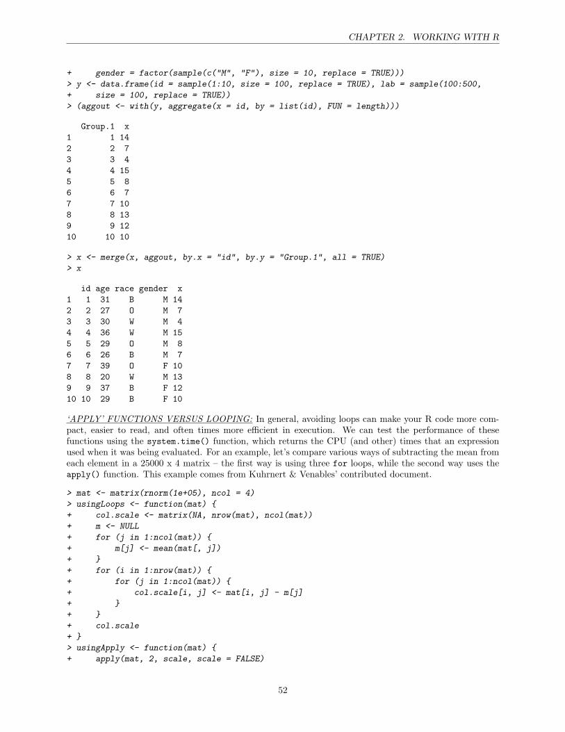
CHAPTER 2. WORKING WITH R
+ gender = factor(sample(c("M", "F"), size = 10, replace = TRUE)))
> y <- data.frame(id = sample(1:10, size = 100, replace = TRUE), lab = sample(100:500,
+ size = 100, replace = TRUE))
> (aggout <- with(y, aggregate(x = id, by = list(id), FUN = length)))
Group.1 x1 1 142 2 73 3 44 4 155 5 86 6 77 7 108 8 139 9 1210 10 10
> x <- merge(x, aggout, by.x = "id", by.y = "Group.1", all = TRUE)
> x
id age race gender x1 1 31 B M 142 2 27 O M 73 3 30 W M 44 4 36 W M 155 5 29 O M 86 6 26 B M 77 7 39 O F 108 8 20 W M 139 9 37 B F 1210 10 29 B F 10
‘APPLY’ FUNCTIONS VERSUS LOOPING: In general, avoiding loops can make your R code more com-pact, easier to read, and often times more efficient in execution. We can test the performance of thesefunctions using the system.time() function, which returns the CPU (and other) times that an expressionused when it was being evaluated. For an example, let’s compare various ways of subtracting the mean fromeach element in a 25000 x 4 matrix – the first way is using three for loops, while the second way uses theapply() function. This example comes from Kuhrnert & Venables’ contributed document.
> mat <- matrix(rnorm(1e+05), ncol = 4)
> usingLoops <- function(mat)
+ col.scale <- matrix(NA, nrow(mat), ncol(mat))
+ m <- NULL
+ for (j in 1:ncol(mat))
+ m[j] <- mean(mat[, j])
+
+ for (i in 1:nrow(mat))
+ for (j in 1:ncol(mat))
+ col.scale[i, j] <- mat[i, j] - m[j]
+
+
+ col.scale
+
> usingApply <- function(mat)
+ apply(mat, 2, scale, scale = FALSE)
52
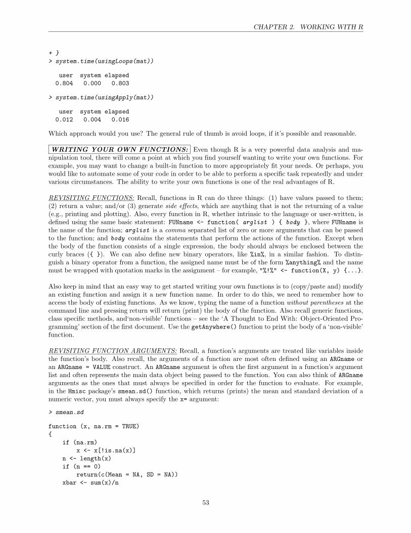
CHAPTER 2. WORKING WITH R
+
> system.time(usingLoops(mat))
user system elapsed0.804 0.000 0.803
> system.time(usingApply(mat))
user system elapsed0.012 0.004 0.016
Which approach would you use? The general rule of thumb is avoid loops, if it’s possible and reasonable.
WRITING YOUR OWN FUNCTIONS: Even though R is a very powerful data analysis and ma-nipulation tool, there will come a point at which you find yourself wanting to write your own functions. Forexample, you may want to change a built-in function to more appropriately fit your needs. Or perhaps, youwould like to automate some of your code in order to be able to perform a specific task repeatedly and undervarious circumstances. The ability to write your own functions is one of the real advantages of R.
REVISITING FUNCTIONS: Recall, functions in R can do three things: (1) have values passed to them;(2) return a value; and/or (3) generate side effects, which are anything that is not the returning of a value(e.g., printing and plotting). Also, every function in R, whether intrinsic to the language or user-written, isdefined using the same basic statement: FUNname <- function( arglist ) body , where FUNname isthe name of the function; arglist is a comma separated list of zero or more arguments that can be passedto the function; and body contains the statements that perform the actions of the function. Except whenthe body of the function consists of a single expression, the body should always be enclosed between thecurly braces ( ). We can also define new binary operators, like %in%, in a similar fashion. To distin-guish a binary operator from a function, the assigned name must be of the form %anything% and the namemust be wrapped with quotation marks in the assignment – for example, "%!%" <- function(X, y) ....
Also keep in mind that an easy way to get started writing your own functions is to (copy/paste and) modifyan existing function and assign it a new function name. In order to do this, we need to remember how toaccess the body of existing functions. As we know, typing the name of a function without parentheses at thecommand line and pressing return will return (print) the body of the function. Also recall generic functions,class specific methods, and‘non-visible’ functions – see the ‘A Thought to End With: Object-Oriented Pro-gramming’ section of the first document. Use the getAnywhere() function to print the body of a ‘non-visible’function.
REVISITING FUNCTION ARGUMENTS: Recall, a function’s arguments are treated like variables insidethe function’s body. Also recall, the arguments of a function are most often defined using an ARGname oran ARGname = VALUE construct. An ARGname argument is often the first argument in a function’s argumentlist and often represents the main data object being passed to the function. You can also think of ARGnamearguments as the ones that must always be specified in order for the function to evaluate. For example,in the Hmisc package’s smean.sd() function, which returns (prints) the mean and standard deviation of anumeric vector, you must always specify the x= argument:
> smean.sd
function (x, na.rm = TRUE)
if (na.rm)x <- x[!is.na(x)]
n <- length(x)if (n == 0)
return(c(Mean = NA, SD = NA))xbar <- sum(x)/n
53
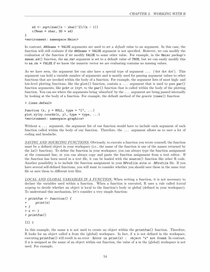
CHAPTER 2. WORKING WITH R
sd <- sqrt(sum((x - xbar)^2)/(n - 1))c(Mean = xbar, SD = sd)
<environment: namespace:Hmisc>
In contrast, ARGname = VALUE arguments are used to set a default value to an argument. In this case, thefunction will still evaluate if the ARGname = VALUE argument is not specified. However, we can modify theevaluation of the function if we modify VALUE to some other value. For example, in the Hmisc package’ssmean.sd() function, the na.rm= argument is set to a default value of TRUE, but we can easily modify thisto na.rm = FALSE if we know the numeric vector we are evaluating contains no missing values.
As we have seen, the argument list can also have a special type of argument ... (‘dot dot dot’). Thisargument can hold a variable number of arguments and is mostly used for passing argument values to otherfunctions that are invoked within the body of a function. For example, the argument lists of most high- andlow-level plotting functions, like the plot() function, contain a ... argument that is used to pass par()function arguments, like pch= or lty=, to the par() function that is called within the body of the plottingfunction. You can see where the arguments being ‘absorbed’ by the ... argument are being passed internallyby looking at the body of a function. For example, the default method of the generic lines() function:
> lines.default
function (x, y = NULL, type = "l", ...)plot.xy(xy.coords(x, y), type = type, ...)<environment: namespace:graphics>
Without a ... argument, the argument list of our function would have to include each argument of eachfunction called within the body of our function. Therefore, the ... argument allows us to save a lot ofcoding and headache.
SAVING AND SOURCING FUNCTIONS: Obviously, to execute a function you wrote yourself, the functionmust be a defined object in your workspace (i.e., the name of the function is one of the names returned bythe ls() function). To define the function in your workspace, you can always type the function assignmentat the command line, or you can always copy and paste the function assignment from a text editor. Ifthe function has been saved in a text file, it can be loaded with the source() function like other R code.Another possibility is to include the function assignment in your RProfile.site or .RProfile file. If youhave several self-defined functions, you will want to consider whether you should save these in the same textfile or save them to different text files.
LOCAL AND GLOBAL VARIABLES IN A FUNCTION: When writing a function, it is not necessary todeclare the variables used within a function. When a function is executed, R uses a rule called lexicalscoping to decide whether an object is local to the function’s body or global (defined in your workspace).To understand this mechanism, let’s consider a very simple function:
> printfun <- function()
+ print(x)
+
> x <- 1
> printfun()
[1] 1
In this example, the name x is not used to create an object within the printfun() function. Therefore,R looks for an object called x from the (global) workspace. In fact, if x is not defined in the workspace,executing printfun() will result in an error – Error in print(x) : object "x" not found. In contrast,if x is assigned as the name of an object within our function, the value of x in the (global) workspace is notused. For example,
54
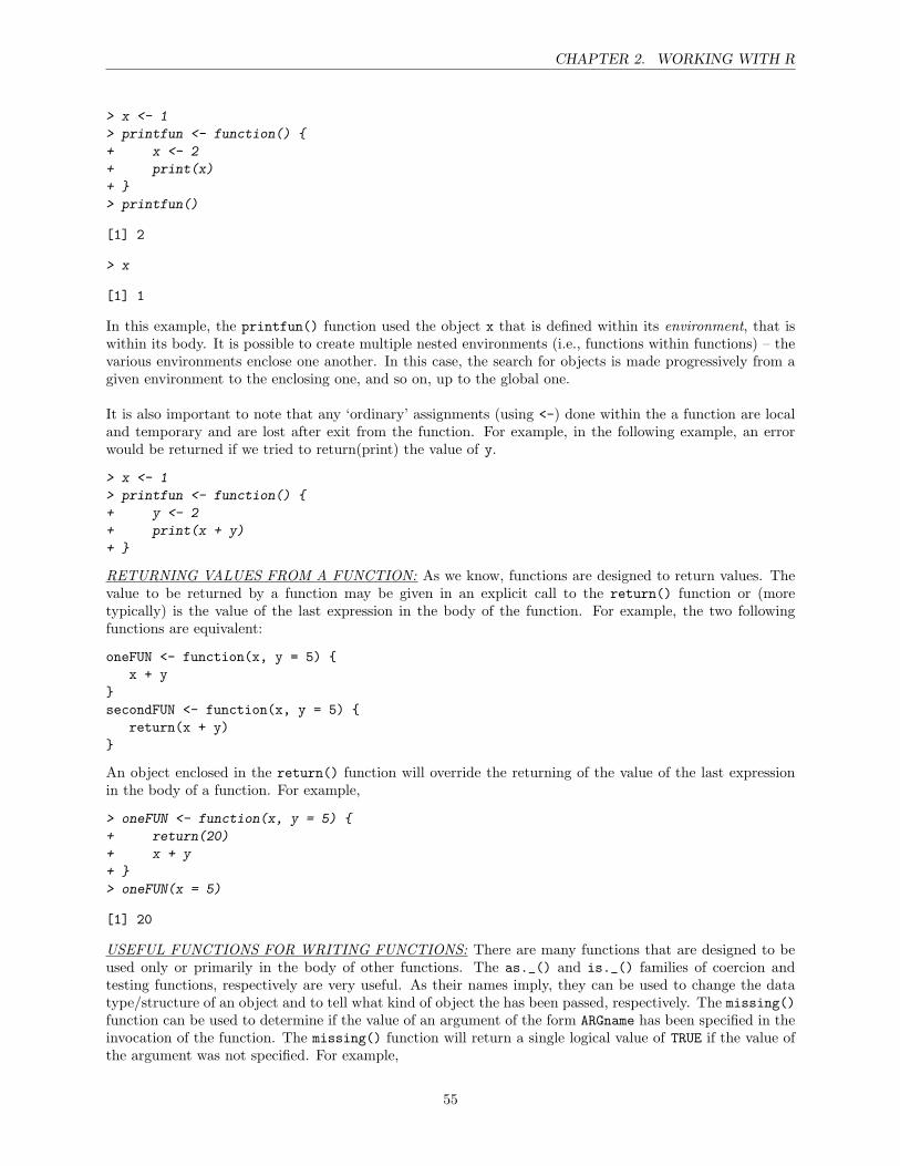
CHAPTER 2. WORKING WITH R
> x <- 1
> printfun <- function()
+ x <- 2
+ print(x)
+
> printfun()
[1] 2
> x
[1] 1
In this example, the printfun() function used the object x that is defined within its environment, that iswithin its body. It is possible to create multiple nested environments (i.e., functions within functions) – thevarious environments enclose one another. In this case, the search for objects is made progressively from agiven environment to the enclosing one, and so on, up to the global one.
It is also important to note that any ‘ordinary’ assignments (using <-) done within the a function are localand temporary and are lost after exit from the function. For example, in the following example, an errorwould be returned if we tried to return(print) the value of y.
> x <- 1
> printfun <- function()
+ y <- 2
+ print(x + y)
+
RETURNING VALUES FROM A FUNCTION: As we know, functions are designed to return values. Thevalue to be returned by a function may be given in an explicit call to the return() function or (moretypically) is the value of the last expression in the body of the function. For example, the two followingfunctions are equivalent:
oneFUN <- function(x, y = 5) x + y
secondFUN <- function(x, y = 5)
return(x + y)
An object enclosed in the return() function will override the returning of the value of the last expressionin the body of a function. For example,
> oneFUN <- function(x, y = 5)
+ return(20)
+ x + y
+
> oneFUN(x = 5)
[1] 20
USEFUL FUNCTIONS FOR WRITING FUNCTIONS: There are many functions that are designed to beused only or primarily in the body of other functions. The as._() and is._() families of coercion andtesting functions, respectively are very useful. As their names imply, they can be used to change the datatype/structure of an object and to tell what kind of object the has been passed, respectively. The missing()function can be used to determine if the value of an argument of the form ARGname has been specified in theinvocation of the function. The missing() function will return a single logical value of TRUE if the value ofthe argument was not specified. For example,
55
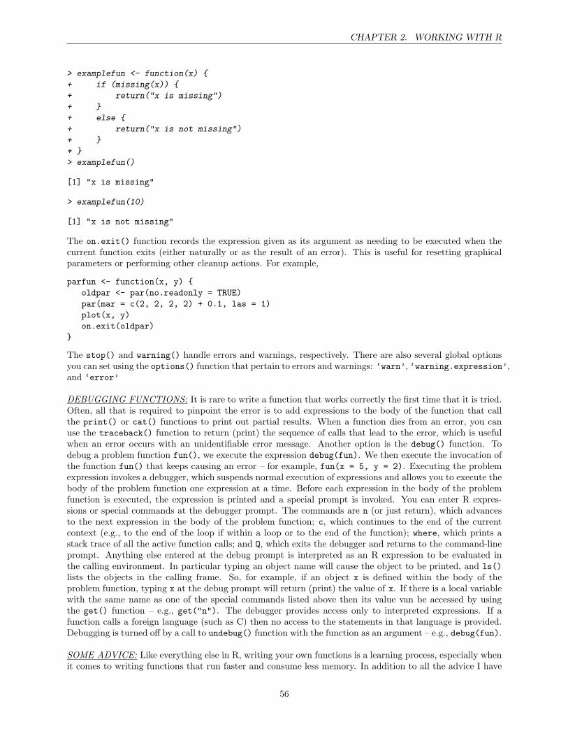
CHAPTER 2. WORKING WITH R
> examplefun <- function(x)
+ if (missing(x))
+ return("x is missing")
+
+ else
+ return("x is not missing")
+
+
> examplefun()
[1] "x is missing"
> examplefun(10)
[1] "x is not missing"
The on.exit() function records the expression given as its argument as needing to be executed when thecurrent function exits (either naturally or as the result of an error). This is useful for resetting graphicalparameters or performing other cleanup actions. For example,
parfun <- function(x, y) oldpar <- par(no.readonly = TRUE)par(mar = c(2, 2, 2, 2) + 0.1, las = 1)plot(x, y)on.exit(oldpar)
The stop() and warning() handle errors and warnings, respectively. There are also several global optionsyou can set using the options() function that pertain to errors and warnings: ‘warn’, ‘warning.expression’,and ‘error’
DEBUGGING FUNCTIONS: It is rare to write a function that works correctly the first time that it is tried.Often, all that is required to pinpoint the error is to add expressions to the body of the function that callthe print() or cat() functions to print out partial results. When a function dies from an error, you canuse the traceback() function to return (print) the sequence of calls that lead to the error, which is usefulwhen an error occurs with an unidentifiable error message. Another option is the debug() function. Todebug a problem function fun(), we execute the expression debug(fun). We then execute the invocation ofthe function fun() that keeps causing an error – for example, fun(x = 5, y = 2). Executing the problemexpression invokes a debugger, which suspends normal execution of expressions and allows you to execute thebody of the problem function one expression at a time. Before each expression in the body of the problemfunction is executed, the expression is printed and a special prompt is invoked. You can enter R expres-sions or special commands at the debugger prompt. The commands are n (or just return), which advancesto the next expression in the body of the problem function; c, which continues to the end of the currentcontext (e.g., to the end of the loop if within a loop or to the end of the function); where, which prints astack trace of all the active function calls; and Q, which exits the debugger and returns to the command-lineprompt. Anything else entered at the debug prompt is interpreted as an R expression to be evaluated inthe calling environment. In particular typing an object name will cause the object to be printed, and ls()lists the objects in the calling frame. So, for example, if an object x is defined within the body of theproblem function, typing x at the debug prompt will return (print) the value of x. If there is a local variablewith the same name as one of the special commands listed above then its value van be accessed by usingthe get() function – e.g., get("n"). The debugger provides access only to interpreted expressions. If afunction calls a foreign language (such as C) then no access to the statements in that language is provided.Debugging is turned off by a call to undebug() function with the function as an argument – e.g., debug(fun).
SOME ADVICE: Like everything else in R, writing your own functions is a learning process, especially whenit comes to writing functions that run faster and consume less memory. In addition to all the advice I have
56
CHAPTER 2. WORKING WITH R
tried to insert in this and the first document, the following is, as John Fox put it, some additional ‘general,miscellaneous, and mostly unoriginal’ advice about writing your own functions.
Work from the bottom up. You will occasionally encounter a moderately large programming project. Itis almost always helpful to break a large project into smaller parts, each of which can be programmed asan independent functions. In a truly complex project, these functions may be organized hierarchically,with some calling others. If some of these small functions are of more general utility, then you canmaintain them as independent functions and reuse them.
Test your program. Before worrying about speed, memory usage, elegance, and so on, make sure thatyour function provides the right answer. Developing any function is an iterative process of refinement,and getting a function to work correctly is the key first step. In checking out your function, try toanticipate all of the circumstances that the function will encounter and test each of them. Furthermore,in ‘quick-and-dirty’ programming, the time that you spend writing and debugging your function willprobably be vastly greater than the time the function spends executing. Remember the programmer’sadage: ‘Make it right before you make it faster.’
Document your functions. The best way to document your functions is to write them in a transparentand readable style – use descriptive function and argument names, even if this means that they arelonger than what you may prefer; name the elements of the various data structures that are createdin the body a function (i.e., x[, "dead"] is more meaningful than x[ , 2]); avoid clever but cryptictricks in your code (trust me, you’ll spend a fair amount of time trying to figure out the trick every timeyou read your code); break long expressions over multiple lines; indent lines (for example, in loops) toreveal the structure; always use parentheses to make groupings explicit; always use curly braces, and, in the body of your functions, including with for, if, else, and other statements; and always useTRUE and FALSE instead of T and F. In addition, if at all possible, give parameters sensible defaults.You can also add a few comments to the beginning of a function to explain what the function doesand what its arguments mean. The key is that you want to understand your own functions when youreturn to them a month or a year later.
57
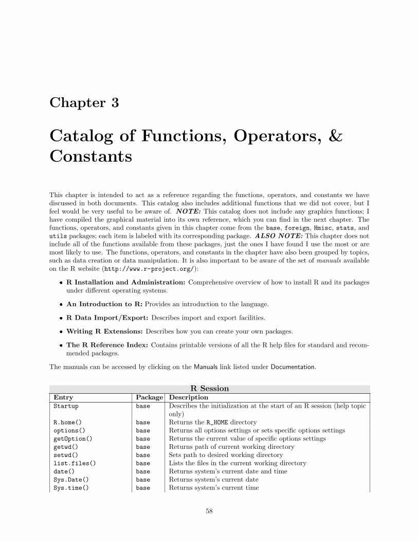
Chapter 3
Catalog of Functions, Operators, &Constants
This chapter is intended to act as a reference regarding the functions, operators, and constants we havediscussed in both documents. This catalog also includes additional functions that we did not cover, but Ifeel would be very useful to be aware of. NOTE: This catalog does not include any graphics functions; Ihave compiled the graphical material into its own reference, which you can find in the next chapter. Thefunctions, operators, and constants given in this chapter come from the base, foreign, Hmisc, stats, andutils packages; each item is labeled with its corresponding package. ALSO NOTE: This chapter does notinclude all of the functions available from these packages, just the ones I have found I use the most or aremost likely to use. The functions, operators, and constants in the chapter have also been grouped by topics,such as data creation or data manipulation. It is also important to be aware of the set of manuals availableon the R website (http://www.r-project.org/):
R Installation and Administration: Comprehensive overview of how to install R and its packagesunder different operating systems.
An Introduction to R: Provides an introduction to the language.
R Data Import/Export: Describes import and export facilities.
Writing R Extensions: Describes how you can create your own packages.
The R Reference Index: Contains printable versions of all the R help files for standard and recom-mended packages.
The manuals can be accessed by clicking on the Manuals link listed under Documentation.
R SessionEntry Package DescriptionStartup base Describes the initialization at the start of an R session (help topic
only)R.home() base Returns the R_HOME directoryoptions() base Returns all options settings or sets specific options settingsgetOption() base Returns the current value of specific options settingsgetwd() base Returns path of current working directorysetwd() base Sets path to desired working directorylist.files() base Lists the files in the current working directorydate() base Returns system’s current date and timeSys.Date() base Returns system’s current dateSys.time() base Returns system’s current time
58
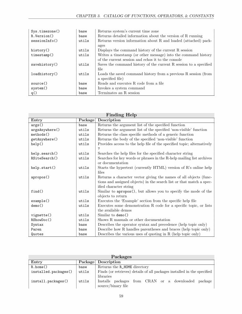
CHAPTER 3. CATALOG OF FUNCTIONS, OPERATORS, & CONSTANTS
Sys.timezone() base Returns system’s current time zoneR.Version() base Returns detailed information about the version of R runningsessionInfo() utils Returns version information about R and loaded (attached) pack-
ageshistory() utils Displays the command history of the current R sessiontimestamp() utils Writes a timestamp (or other message) into the command history
of the current session and echos it to the consolesavehistory() utils Saves the command history of the current R session to a specified
fileloadhistory() utils Loads the saved command history from a previous R session (from
a specified file)source() base Reads and executes R code from a filesystem() base Invokes a system commandq() base Terminates an R session
Finding HelpEntry Package Descriptionargs() base Returns the argument list of the specified functionargsAnywhere() utils Returns the argument list of the specified ‘non-visible’ functionmethods() utils Returns the class specific methods of a generic functiongetAnywhere() utils Returns the body of the specified ‘non-visible’ functionhelp() utils Provides access to the help file of the specified topic; alternatively
?help.search() utils Searches the help files for the specified character stringRSiteSearch() utils Searches for key words or phrases in the R-help mailing list archives
or documentationhelp.start() utils Starts the hypertext (currently HTML) version of R’s online help
filesapropos() utils Returns a character vector giving the names of all objects (func-
tions and assigned objects) in the search list or that match a spec-ified character string
find() utils Similar to apropos(), but allows you to specify the mode of theobjects to return
example() utils Executes the ‘Example’ section from the specific help filedemo() utils Executes some demonstration R code for a specific topic, or lists
the available demosvignette() utils Similar to demo()RShowDoc() utils Shows R manuals or other documentationSyntax base Describes the operator syntax and precedence (help topic only)Paren base Describe how R handles parentheses and braces (help topic only)Quotes base Describes the various uses of quoting in R (help topic only)
PackagesEntry Package DescriptionR.home() base Returns the R_HOME directoryinstalled.packages() utils Finds (or retrieves) details of all packages installed in the specified
librariesinstall.packages() utils Installs packages from CRAN or a downloaded package
source/binary file
59
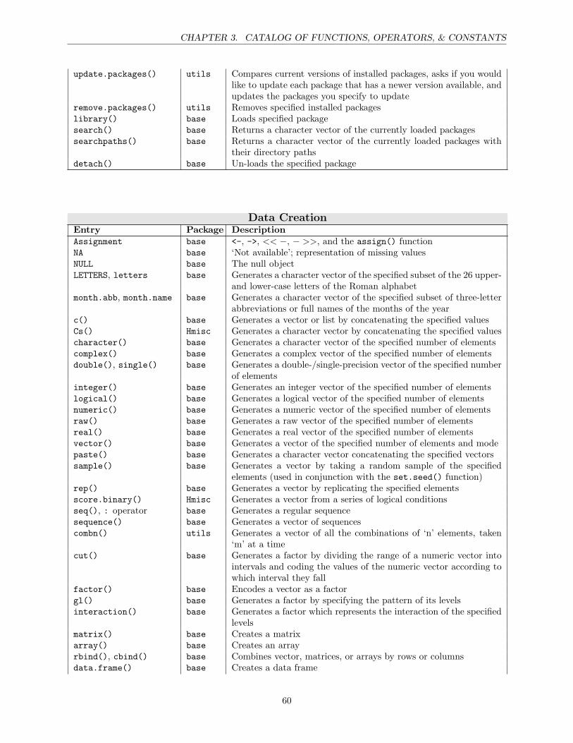
CHAPTER 3. CATALOG OF FUNCTIONS, OPERATORS, & CONSTANTS
update.packages() utils Compares current versions of installed packages, asks if you wouldlike to update each package that has a newer version available, andupdates the packages you specify to update
remove.packages() utils Removes specified installed packageslibrary() base Loads specified packagesearch() base Returns a character vector of the currently loaded packagessearchpaths() base Returns a character vector of the currently loaded packages with
their directory pathsdetach() base Un-loads the specified package
Data CreationEntry Package DescriptionAssignment base <-, ->, << −, − >>, and the assign() functionNA base ‘Not available’; representation of missing valuesNULL base The null objectLETTERS, letters base Generates a character vector of the specified subset of the 26 upper-
and lower-case letters of the Roman alphabetmonth.abb, month.name base Generates a character vector of the specified subset of three-letter
abbreviations or full names of the months of the yearc() base Generates a vector or list by concatenating the specified valuesCs() Hmisc Generates a character vector by concatenating the specified valuescharacter() base Generates a character vector of the specified number of elementscomplex() base Generates a complex vector of the specified number of elementsdouble(), single() base Generates a double-/single-precision vector of the specified number
of elementsinteger() base Generates an integer vector of the specified number of elementslogical() base Generates a logical vector of the specified number of elementsnumeric() base Generates a numeric vector of the specified number of elementsraw() base Generates a raw vector of the specified number of elementsreal() base Generates a real vector of the specified number of elementsvector() base Generates a vector of the specified number of elements and modepaste() base Generates a character vector concatenating the specified vectorssample() base Generates a vector by taking a random sample of the specified
elements (used in conjunction with the set.seed() function)rep() base Generates a vector by replicating the specified elementsscore.binary() Hmisc Generates a vector from a series of logical conditionsseq(), : operator base Generates a regular sequencesequence() base Generates a vector of sequencescombn() utils Generates a vector of all the combinations of ‘n’ elements, taken
‘m’ at a timecut() base Generates a factor by dividing the range of a numeric vector into
intervals and coding the values of the numeric vector according towhich interval they fall
factor() base Encodes a vector as a factorgl() base Generates a factor by specifying the pattern of its levelsinteraction() base Generates a factor which represents the interaction of the specified
levelsmatrix() base Creates a matrixarray() base Creates an arrayrbind(), cbind() base Combines vector, matrices, or arrays by rows or columnsdata.frame() base Creates a data frame
60
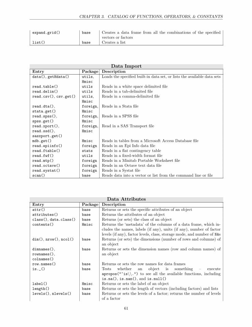
CHAPTER 3. CATALOG OF FUNCTIONS, OPERATORS, & CONSTANTS
expand.grid() base Creates a data frame from all the combinations of the specifiedvectors or factors
list() base Creates a list
Data ImportEntry Package Descriptiondata(), getHdata() utils,
HmiscLoads the specified built-in data set, or lists the available data sets
read.table() utils Reads in a white space delimited fileread.delim() utils Reads in a tab-delimited fileread.csv(), csv.get() utils,
HmiscReads in a comma-delimited file
read.dta(),stata.get()
foreign,Hmisc
Reads in a Stata file
read.spss(),spss.get()
foreign,Hmisc
Reads in a SPSS file
read.xport(),read.ssd(),sasxport.get()
foreign,Hmisc
Read in a SAS Transport file
mdb.get() Hmisc Reads in tables from a Microsoft Access Database fileread.epiinfo() foreign Reads in an Epi Info data fileread.ftable() stats Reads in a flat contingency tableread.fwf() utils Reads in a fixed-width format fileread.mtp() foreign Reads in a Minitab Portable Worksheet fileread.octave() foreign Reads in an Octave text data fileread.systat() foreign Reads in a Systat filescan() base Reads data into a vector or list from the command line or file
Data AttributesEntry Package Descriptionattr() base Returns or sets the specific attributes of an objectattributes() base Returns the attributes of an objectclass(), data.class() base Returns (or sets) the class of an objectcontents() Hmisc Returns the ‘metadata’ of the columns of a data frame, which in-
cludes the names, labels (if any), units (if any), number of factorlevels (if any), factor levels, class, storage mode, and number of NAs
dim(), nrow(), ncol() base Returns (or sets) the dimensions (number of rows and columns) ofan object
dimnames(),rownames(),colnames()
base Returns or sets the dimension names (row and column names) ofan object
row.names() base Returns or sets the row names for data framesis._() base Tests whether an object is something – execute
apropos("^is\\.") to see all the available functions, includingis.na(), is.nan(), and is.null()
label() Hmisc Returns or sets the label of an objectlength() base Returns or sets the length of vectors (including factors) and listslevels(), nlevels() base Returns or sets the levels of a factor; returns the number of levels
of a factor
61
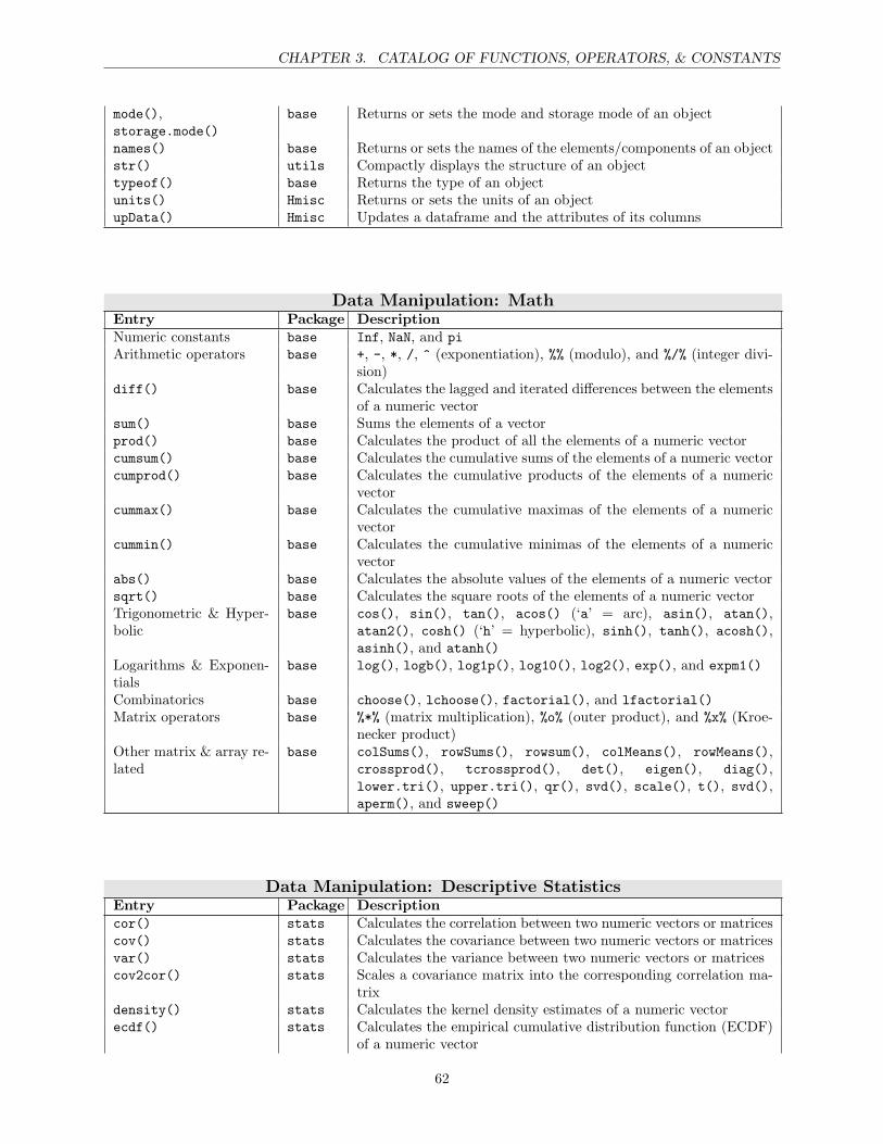
CHAPTER 3. CATALOG OF FUNCTIONS, OPERATORS, & CONSTANTS
mode(),storage.mode()
base Returns or sets the mode and storage mode of an object
names() base Returns or sets the names of the elements/components of an objectstr() utils Compactly displays the structure of an objecttypeof() base Returns the type of an objectunits() Hmisc Returns or sets the units of an objectupData() Hmisc Updates a dataframe and the attributes of its columns
Data Manipulation: MathEntry Package DescriptionNumeric constants base Inf, NaN, and piArithmetic operators base +, -, *, /, ^ (exponentiation), %% (modulo), and %/% (integer divi-
sion)diff() base Calculates the lagged and iterated differences between the elements
of a numeric vectorsum() base Sums the elements of a vectorprod() base Calculates the product of all the elements of a numeric vectorcumsum() base Calculates the cumulative sums of the elements of a numeric vectorcumprod() base Calculates the cumulative products of the elements of a numeric
vectorcummax() base Calculates the cumulative maximas of the elements of a numeric
vectorcummin() base Calculates the cumulative minimas of the elements of a numeric
vectorabs() base Calculates the absolute values of the elements of a numeric vectorsqrt() base Calculates the square roots of the elements of a numeric vectorTrigonometric & Hyper-bolic
base cos(), sin(), tan(), acos() (‘a’ = arc), asin(), atan(),atan2(), cosh() (‘h’ = hyperbolic), sinh(), tanh(), acosh(),asinh(), and atanh()
Logarithms & Exponen-tials
base log(), logb(), log1p(), log10(), log2(), exp(), and expm1()
Combinatorics base choose(), lchoose(), factorial(), and lfactorial()Matrix operators base %*% (matrix multiplication), %o% (outer product), and %x% (Kroe-
necker product)Other matrix & array re-lated
base colSums(), rowSums(), rowsum(), colMeans(), rowMeans(),crossprod(), tcrossprod(), det(), eigen(), diag(),lower.tri(), upper.tri(), qr(), svd(), scale(), t(), svd(),aperm(), and sweep()
Data Manipulation: Descriptive StatisticsEntry Package Descriptioncor() stats Calculates the correlation between two numeric vectors or matricescov() stats Calculates the covariance between two numeric vectors or matricesvar() stats Calculates the variance between two numeric vectors or matricescov2cor() stats Scales a covariance matrix into the corresponding correlation ma-
trixdensity() stats Calculates the kernel density estimates of a numeric vectorecdf() stats Calculates the empirical cumulative distribution function (ECDF)
of a numeric vector
62
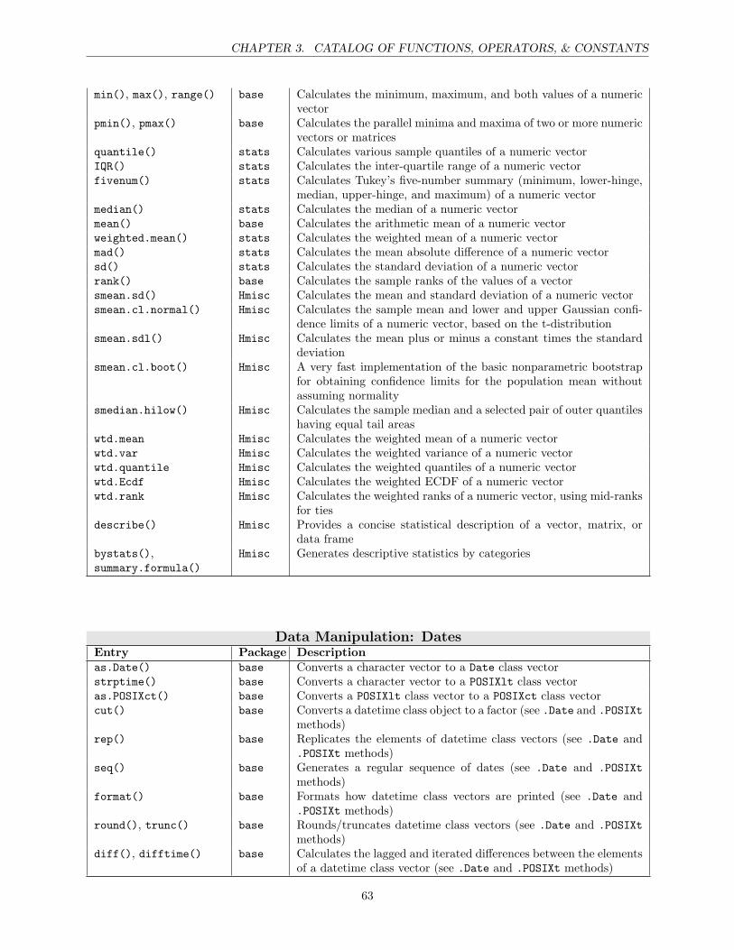
CHAPTER 3. CATALOG OF FUNCTIONS, OPERATORS, & CONSTANTS
min(), max(), range() base Calculates the minimum, maximum, and both values of a numericvector
pmin(), pmax() base Calculates the parallel minima and maxima of two or more numericvectors or matrices
quantile() stats Calculates various sample quantiles of a numeric vectorIQR() stats Calculates the inter-quartile range of a numeric vectorfivenum() stats Calculates Tukey’s five-number summary (minimum, lower-hinge,
median, upper-hinge, and maximum) of a numeric vectormedian() stats Calculates the median of a numeric vectormean() base Calculates the arithmetic mean of a numeric vectorweighted.mean() stats Calculates the weighted mean of a numeric vectormad() stats Calculates the mean absolute difference of a numeric vectorsd() stats Calculates the standard deviation of a numeric vectorrank() base Calculates the sample ranks of the values of a vectorsmean.sd() Hmisc Calculates the mean and standard deviation of a numeric vectorsmean.cl.normal() Hmisc Calculates the sample mean and lower and upper Gaussian confi-
dence limits of a numeric vector, based on the t-distributionsmean.sdl() Hmisc Calculates the mean plus or minus a constant times the standard
deviationsmean.cl.boot() Hmisc A very fast implementation of the basic nonparametric bootstrap
for obtaining confidence limits for the population mean withoutassuming normality
smedian.hilow() Hmisc Calculates the sample median and a selected pair of outer quantileshaving equal tail areas
wtd.mean Hmisc Calculates the weighted mean of a numeric vectorwtd.var Hmisc Calculates the weighted variance of a numeric vectorwtd.quantile Hmisc Calculates the weighted quantiles of a numeric vectorwtd.Ecdf Hmisc Calculates the weighted ECDF of a numeric vectorwtd.rank Hmisc Calculates the weighted ranks of a numeric vector, using mid-ranks
for tiesdescribe() Hmisc Provides a concise statistical description of a vector, matrix, or
data framebystats(),summary.formula()
Hmisc Generates descriptive statistics by categories
Data Manipulation: DatesEntry Package Descriptionas.Date() base Converts a character vector to a Date class vectorstrptime() base Converts a character vector to a POSIXlt class vectoras.POSIXct() base Converts a POSIXlt class vector to a POSIXct class vectorcut() base Converts a datetime class object to a factor (see .Date and .POSIXt
methods)rep() base Replicates the elements of datetime class vectors (see .Date and
.POSIXt methods)seq() base Generates a regular sequence of dates (see .Date and .POSIXt
methods)format() base Formats how datetime class vectors are printed (see .Date and
.POSIXt methods)round(), trunc() base Rounds/truncates datetime class vectors (see .Date and .POSIXt
methods)diff(), difftime() base Calculates the lagged and iterated differences between the elements
of a datetime class vector (see .Date and .POSIXt methods)
63
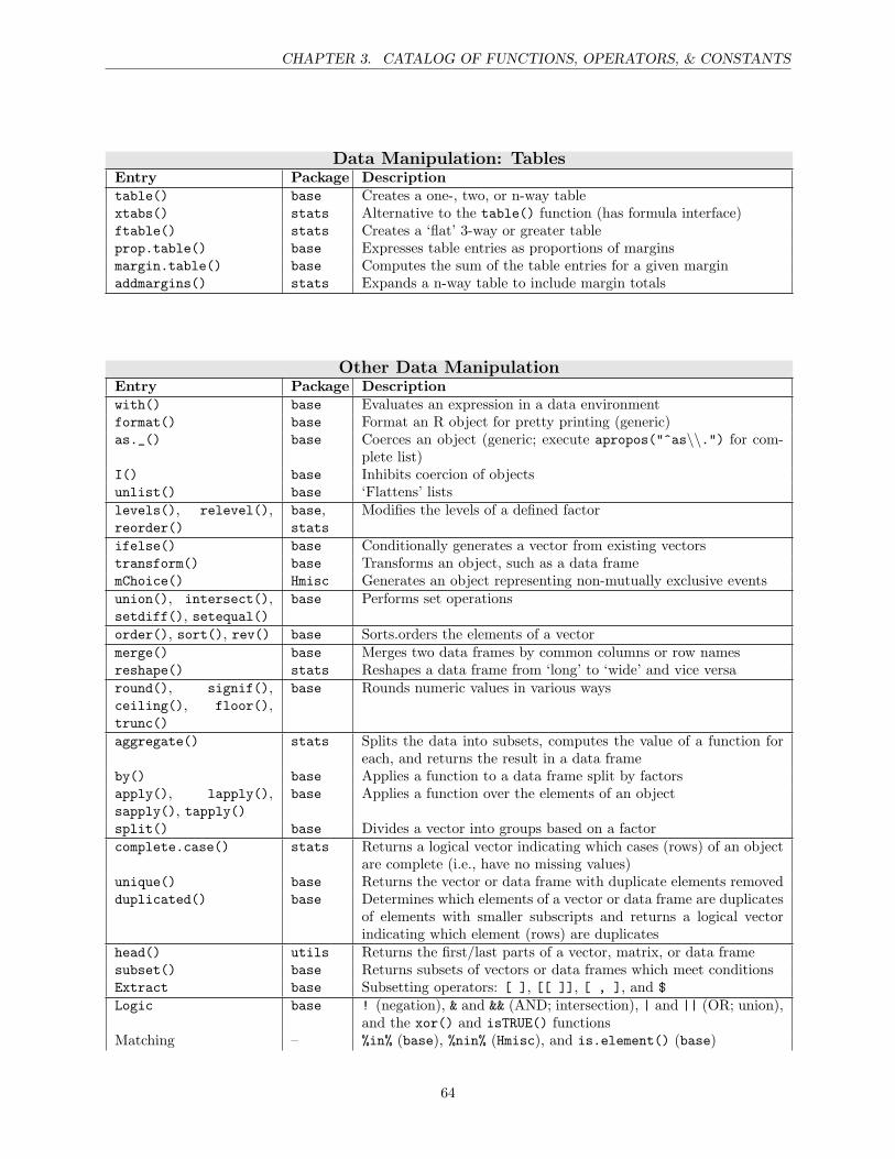
CHAPTER 3. CATALOG OF FUNCTIONS, OPERATORS, & CONSTANTS
Data Manipulation: TablesEntry Package Descriptiontable() base Creates a one-, two, or n-way tablextabs() stats Alternative to the table() function (has formula interface)ftable() stats Creates a ‘flat’ 3-way or greater tableprop.table() base Expresses table entries as proportions of marginsmargin.table() base Computes the sum of the table entries for a given marginaddmargins() stats Expands a n-way table to include margin totals
Other Data ManipulationEntry Package Descriptionwith() base Evaluates an expression in a data environmentformat() base Format an R object for pretty printing (generic)as._() base Coerces an object (generic; execute apropos("^as\\.") for com-
plete list)I() base Inhibits coercion of objectsunlist() base ‘Flattens’ listslevels(), relevel(),reorder()
base,stats
Modifies the levels of a defined factor
ifelse() base Conditionally generates a vector from existing vectorstransform() base Transforms an object, such as a data framemChoice() Hmisc Generates an object representing non-mutually exclusive eventsunion(), intersect(),setdiff(), setequal()
base Performs set operations
order(), sort(), rev() base Sorts.orders the elements of a vectormerge() base Merges two data frames by common columns or row namesreshape() stats Reshapes a data frame from ‘long’ to ‘wide’ and vice versaround(), signif(),ceiling(), floor(),trunc()
base Rounds numeric values in various ways
aggregate() stats Splits the data into subsets, computes the value of a function foreach, and returns the result in a data frame
by() base Applies a function to a data frame split by factorsapply(), lapply(),sapply(), tapply()
base Applies a function over the elements of an object
split() base Divides a vector into groups based on a factorcomplete.case() stats Returns a logical vector indicating which cases (rows) of an object
are complete (i.e., have no missing values)unique() base Returns the vector or data frame with duplicate elements removedduplicated() base Determines which elements of a vector or data frame are duplicates
of elements with smaller subscripts and returns a logical vectorindicating which element (rows) are duplicates
head() utils Returns the first/last parts of a vector, matrix, or data framesubset() base Returns subsets of vectors or data frames which meet conditionsExtract base Subsetting operators: [ ], [[ ]], [ , ], and $Logic base ! (negation), & and && (AND; intersection), | and || (OR; union),
and the xor() and isTRUE() functionsMatching – %in% (base), %nin% (Hmisc), and is.element() (base)
64
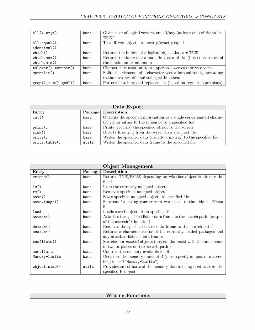
CHAPTER 3. CATALOG OF FUNCTIONS, OPERATORS, & CONSTANTS
all(), any() base Given a set of logical vectors, are all/any (at least one) of the valuesTRUE?
all.equal(),identical()
base Tests if two objects are nearly/exactly equal
which() base Returns the indices of a logical object that are TRUEwhich.max(),which.min()
base Returns the indices of a numeric vector of the (first) occurrence ofthe maximum or minimum
tolower(), toupper() base Character translation from upper to lower case or vice versastrsplit() base Splits the elements of a character vector into substrings according
to the presence of a substring within themgrep(), sub(), gsub() base Pattern matching and replacement (based on regular expressions)
Data ExportEntry Package Descriptioncat() base Outputs the specified information as a single concatenated charac-
ter vector either to the screen or to a specified fileprint() base Prints (returns) the specified object to the screensink() base Diverts R output from the screen to a specified filewrite() base Writes the specified data (usually a matrix) to the specified filewrite.table() utils Writes the specified data frame to the specified file
Object ManagementEntry Package Descriptionexists() base Returns TRUE/FALSE depending on whether object is already de-
finedls() base Lists the currently assigned objectsrm() base Removes specified assigned objectssave() base Saves specified assigned objects to specified filesave.image() base Shortcut for saving your current workspace to the hidden .RData
fileload base Loads saved objects from specified fileattach() base Attaches the specified list or data frame to the ‘search path’ (output
of the search() function)detach() base Removes the specified list or data frame to the ‘search path’search() base Returns a character vector of the currently loaded packages and
any attached lists or data framesconflicts() base Searches for masked objects (objects that exist with the same name
in two or places on the ‘search path’)mem.limits base Controls the memory available for RMemory-limits base Describes the memory limits of R (must specify in quotes to access
help file – ?"Memory-limits")object.size() utils Provides an estimate of the memory that is being used to store the
specified R object
Writing Functions
65

CHAPTER 3. CATALOG OF FUNCTIONS, OPERATORS, & CONSTANTS
Entry Package DescriptionAssignment base <-, ->, << −, − >>, and the assign() functionalarm() utils Gives an audible or visual signal to the usermissing() base Tests whether a value was specified for a specific argument to a
functionmatch.arg() base Matches the argument specified against a table of candidate valuesmatch.call()do.call()
base Constructs and executes a function call from a name or a functionand a list of arguments to be passed to it
Repetitive & Conditionalevaluation
base if, else, for, while, repeat, break, next (must specify in quotesto access help file – ?"for"), and the switch() function
stop() base Stops the execution of the current expression and executes an erroraction
warning() base Generates a warning message that corresponds to its argument(s)require() base Loads the specified package if not already done sotempfile() base Creates names for temporary filesreturn() base Returns a value from a functioninvisible() base Returns a (temporarily) invisible copy of an objecton.exit() base Records the expression given as its argument as needing to be ex-
ecuted when the current function exits (either naturally or as theresult of an error)
traceback() base Prints the sequence of calls that lead to the error of a functiondebug() base Debugs a functionRprof() utils Profiles the execution of R expressions
66
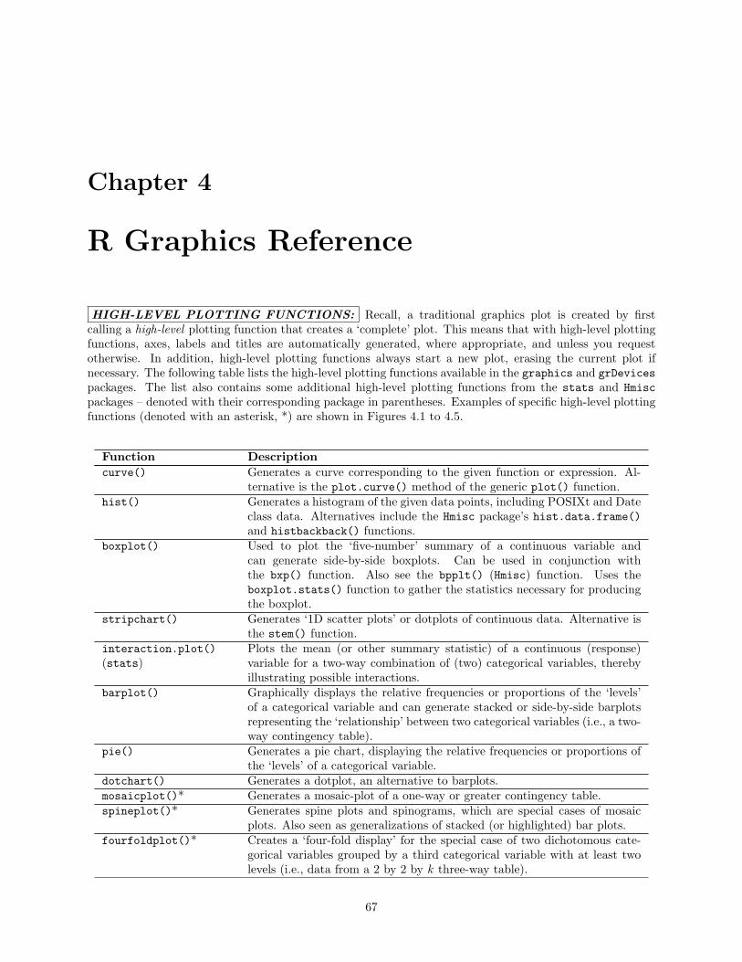
Chapter 4
R Graphics Reference
HIGH-LEVEL PLOTTING FUNCTIONS: Recall, a traditional graphics plot is created by firstcalling a high-level plotting function that creates a ‘complete’ plot. This means that with high-level plottingfunctions, axes, labels and titles are automatically generated, where appropriate, and unless you requestotherwise. In addition, high-level plotting functions always start a new plot, erasing the current plot ifnecessary. The following table lists the high-level plotting functions available in the graphics and grDevicespackages. The list also contains some additional high-level plotting functions from the stats and Hmiscpackages – denoted with their corresponding package in parentheses. Examples of specific high-level plottingfunctions (denoted with an asterisk, *) are shown in Figures 4.1 to 4.5.
Function Descriptioncurve() Generates a curve corresponding to the given function or expression. Al-
ternative is the plot.curve() method of the generic plot() function.hist() Generates a histogram of the given data points, including POSIXt and Date
class data. Alternatives include the Hmisc package’s hist.data.frame()and histbackback() functions.
boxplot() Used to plot the ‘five-number’ summary of a continuous variable andcan generate side-by-side boxplots. Can be used in conjunction withthe bxp() function. Also see the bpplt() (Hmisc) function. Uses theboxplot.stats() function to gather the statistics necessary for producingthe boxplot.
stripchart() Generates ‘1D scatter plots’ or dotplots of continuous data. Alternative isthe stem() function.
interaction.plot()(stats)
Plots the mean (or other summary statistic) of a continuous (response)variable for a two-way combination of (two) categorical variables, therebyillustrating possible interactions.
barplot() Graphically displays the relative frequencies or proportions of the ‘levels’of a categorical variable and can generate stacked or side-by-side barplotsrepresenting the ‘relationship’ between two categorical variables (i.e., a two-way contingency table).
pie() Generates a pie chart, displaying the relative frequencies or proportions ofthe ‘levels’ of a categorical variable.
dotchart() Generates a dotplot, an alternative to barplots.mosaicplot()* Generates a mosaic-plot of a one-way or greater contingency table.spineplot()* Generates spine plots and spinograms, which are special cases of mosaic
plots. Also seen as generalizations of stacked (or highlighted) bar plots.fourfoldplot()* Creates a ‘four-fold display’ for the special case of two dichotomous cate-
gorical variables grouped by a third categorical variable with at least twolevels (i.e., data from a 2 by 2 by k three-way table).
67

CHAPTER 4. R GRAPHICS REFERENCE
assocplot()* Produces a Cohen-Friendly association plot indicating deviations from in-dependence of the rows and columns in a two-way contingency table.
cdplot()* Computes and plots the conditional densities describing how the conditionaldistribution of a categorical variable y changes over a numeric variable x.
plot() Generic. The default method (plot.default()) produces a basic scat-ter plot between two continuous variables. Can also handle variables ofPOSIXct, POSIXlt, and Date class. Invoke methods(plot) to list all classspecific methods.
scatter.smooth()(stats)
Generates an x-y scatterplot with smooth curves fitted by LOESS.
persp()* Useful to graphically display three continuous variables. Generates an x-yscatterplot between two of the continuous variables and represents the thirdcontinuous variable by generating a 3D surface over the x-y plane.
contour()* Useful to graphically display three continuous variables. Generates anx-y scatterplot between two of the continuous variables and representsthe third continuous variable using contour lines. Alternative is thefilled.contour() function.
symbols()* Useful to graphically display three continuous variables. Generates an x-yscatterplot between two of the continuous variables and represents the thirdcontinuous variable using a symbol (e.g., circles of varying radius).
image()* Useful to graphically display three continuous variables. Produces an x-ygrid of rectangles and uses color to represent the value of a third variablez.
pairs() Generates a matrix of scatterplots, plotting each continuous variables byall other continuous variables specified. Can be used in conjunction withthe panel.smooth() function.
stars()* Generates star (spider/radar) plots or segments diagrams of a multivariatedata set.
coplot()* Produces two types of conditioning plots.matplot() Plots the columns of one matrix against the columns of another.heatmap()* (stats) Draws a heat map, which is a false color image (basically image(t(x))),
with a dendrogram added to the left side and top.sunflowerplot()* Useful when identical data values repeat a small number of times. Plots a
‘flower’ at each x-y location with a ‘petal’ for each replication of z.
‘STANDARD’ ARGUMENTS OF HIGH-LEVEL PLOTTING FUNCTIONS: Recall, in addition to function-specific arguments, there are several arguments that are ‘standard’ in the sense that many high-level plottingfunctions will accept them. Specifically, most high-level plotting functions will accept graphical parameterarguments that control such things as the appearance of axes and labels, and the range of the axes scales.It is usually possible to modify the default range of the axes scales on a plot by specifying the xlim= and/orylim= arguments in the high-level function invocation, which are each specified as two element vectors con-taining the minimum and maximum values (e.g., xlim = c(0, 50)). There is also a set of arguments formodifying the default labels (if any) on a plot: main= for a title, sub= for a sub-title, xlab= for an x-axislabel, and ylab= for a y-axis label. Each of these arguments is specified as a character string. The titlespecified with the main= argument (if any) is placed at the top of the plot in a large font, and the sub-titlespecified with the sub= argument is placed just below the x-axis in a smaller font. Some high-level plottingfunctions have an axes= argument (by default TRUE), which allows (if set to FALSE) you to suppress thedrawing of the axes and therefore produce customized axes instead. Lastly, some high-level plotting functionhave an add= argument (by default FALSE), which, if set to TRUE, forces the function to act as a low-levelplotting, superimposing the high-level plot onto the current plot.
68

CHAPTER 4. R GRAPHICS REFERENCE
Figure 4.1: Examples of high-level plotting functions – mosaicplot(), spineplot(), fourfoldplot(), andassocplot().
mosaicplot()
Treatment
Col
laps
ed S
urvi
val S
tatu
s D−penicillamine Placebo
Cen
sore
dD
ead
spineplot()
Treatment
Col
laps
ed S
urvi
val S
tatu
s
D−penicillamine Placebo
Cen
sore
dD
ead
0.0
0.2
0.4
0.6
0.8
1.0
sex: Female
drug
: D−
peni
cilla
min
e
sex: Male
drug
: Pla
cebo
stage: 1
4
0
1
0
sex: Female
drug
: D−
peni
cilla
min
e
sex: Male
drug
: Pla
cebo
stage: 2
7
2
7
1
sex: Female
drug
: D−
peni
cilla
min
e
sex: Male
drug
: Pla
cebo
stage: 3
13
3
10
2
sex: Female
drug
: D−
peni
cilla
min
e
sex: Male
drug
: Pla
cebo
stage: 4
10
1
12
2
fourfoldplot()
1 2 3 4
Dea
dC
enso
red
assocplot()
Histologic stage of disease
Col
laps
ed S
urvi
val S
tatu
s
69

CHAPTER 4. R GRAPHICS REFERENCE
Figure 4.2: Examples of high-level plotting functions – cdplot(), sunflowerplot(), and stars().
cdplot()
Age
Col
laps
ed S
urvi
val S
tatu
s
40 50 60 70
Cen
sore
dD
ead
0.0
0.4
0.8
−2 −1 0 1 2
−3
−1
01
2
sunflowerplot()
X
Y
stars()
mpg
cyl
disp
hp
stars()
Mazda RX4Mazda RX4 Wag
Datsun 710
Hornet 4 DriveHornet Sportabout
Valiant
Duster 360Merc 240D
Merc 230
Merc 280
70
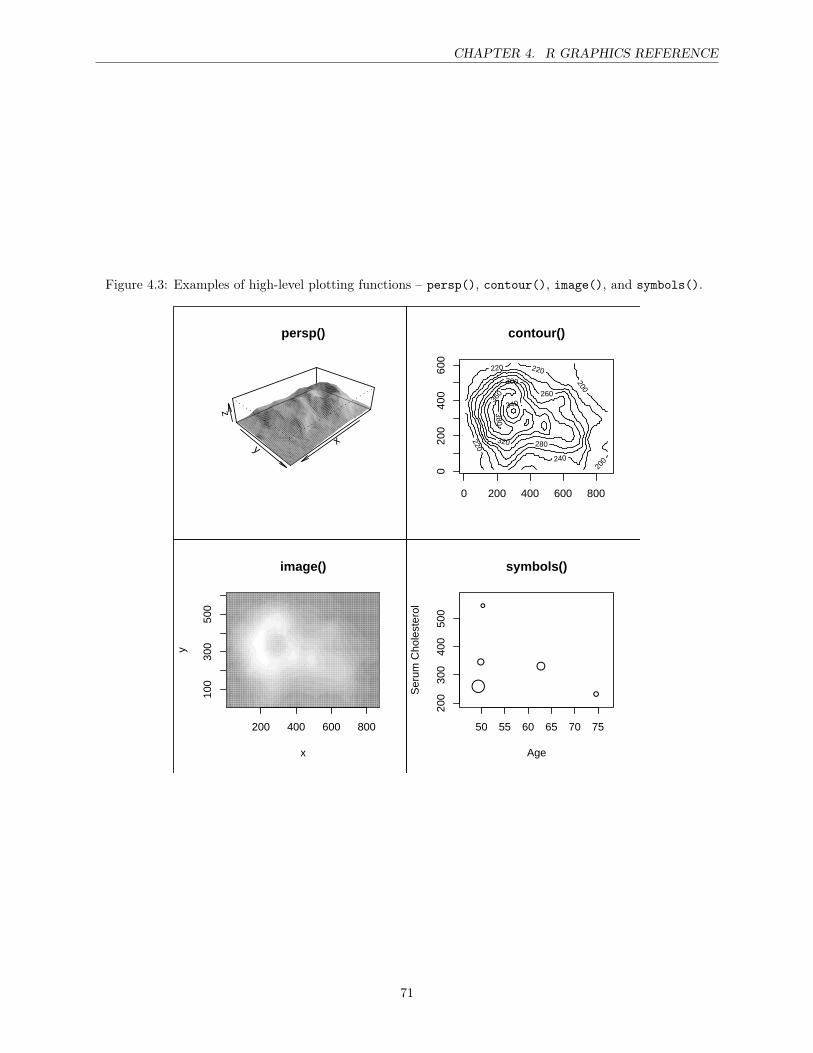
CHAPTER 4. R GRAPHICS REFERENCE
Figure 4.3: Examples of high-level plotting functions – persp(), contour(), image(), and symbols().
xy
z
persp() contour()
200
200
220
220 220
240
260
280
300
320
340 360
380
0 200 400 600 800
020
040
060
0
200 400 600 800
100
300
500
image()
x
y
50 55 60 65 70 75
200
300
400
500
symbols()
Age
Ser
um C
hole
ster
ol
71
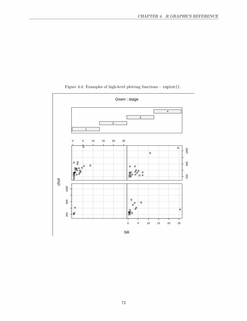
CHAPTER 4. R GRAPHICS REFERENCE
Figure 4.4: Examples of high-level plotting functions – coplot().
200
600
1000
0 5 10 15 20 25
0 5 10 15 20 25
200
600
1000
bili
chol
1
2
3
4
Given : stage
72
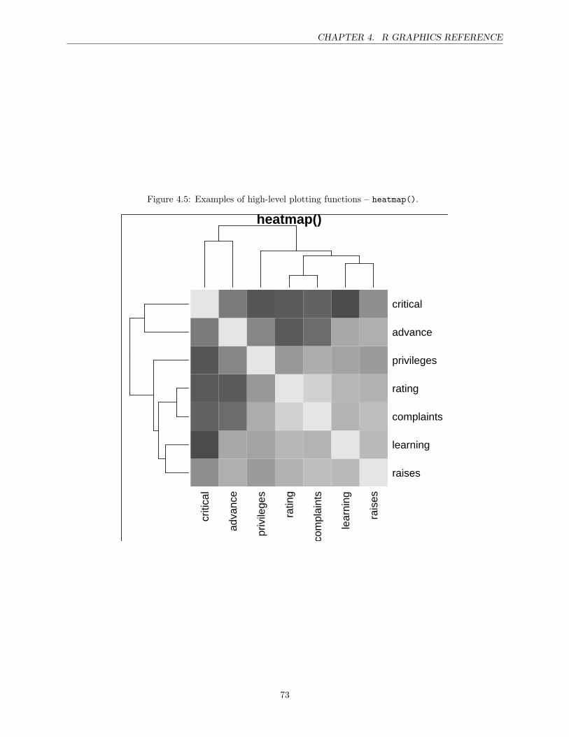
CHAPTER 4. R GRAPHICS REFERENCE
Figure 4.5: Examples of high-level plotting functions – heatmap().cr
itica
l
adva
nce
priv
ilege
s
ratin
g
com
plai
nts
lear
ning
rais
es
raises
learning
complaints
rating
privileges
advance
critical
heatmap()
73
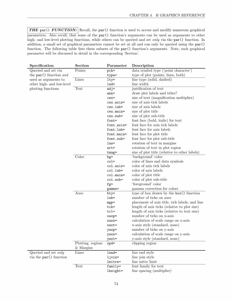
CHAPTER 4. R GRAPHICS REFERENCE
THE par() FUNCTION: Recall, the par() function is used to access and modify numerous graphicalparameters. Also recall, that some of the par() function’s arguments can be used as arguments to otherhigh- and low-level plotting functions, while others can be queried and set only via the par() function. Inaddition, a small set of graphical parameters cannot be set at all and can only be queried using the par()function. The following table lists these subsets of the par() function’s arguments. Note, each graphicalparameter will be discussed in detail in the corresponding ‘Section’.
Specification Section Parameter DescriptionQueried and set via Points pch= data symbol type (‘point character’)the par() function and type= type of plot (points, lines, both)used as arguments to Lines lty= line type (solid, dashed)other high- and low-level lwd= line widthplotting functions Text adj= justification of text
ann= draw plot labels and titles?cex= size of text (magnification multiplier)cex.axis= size of axis tick labelscex.lab= size of axis labelscex.main= size of plot titlecex.sub= size of plot sub-titlefont= font face (bold, italic) for textfont.axis= font face for axis tick labelsfont.lab= font face for axis labelsfont.main= font face for plot titlefont.sub= font face for plot sub-titlelas= rotation of text in marginssrt= rotation of text in plot regiontmag= size of plot title (relative to other labels)
Color bg= ‘background’ colorcol= color of lines and data symbolscol.axis= color of axis tick labelscol.lab= color of axis labelscol.main= color of plot titlecol.sub= color of plot sub-titlefg= ‘foreground’ colorgamma= gamma correction for colors
Axes bty= type of box drawn by the box() functionlab= number of ticks on axesmgp= placement of axis title, tick labels, and linetck= length of axis ticks (relative to plot size)tcl= length of axis ticks (relative to text size)xaxp= number of ticks on x-axisxaxs= calculation of scale range on x-axisxaxt= x-axis style (standard, none)yaxp= number of ticks on y-axisyaxs= calculation of scale range on y-axisyaxt= y-axis style (standard, none)
Plotting regions& Margins
xpd= clipping region
Queried and set only Lines lend= line end stylevia the par() function ljoin= line join style
lmitre= line mitre limitText family= font family for text
lheight= line spacing (multiplier)
74
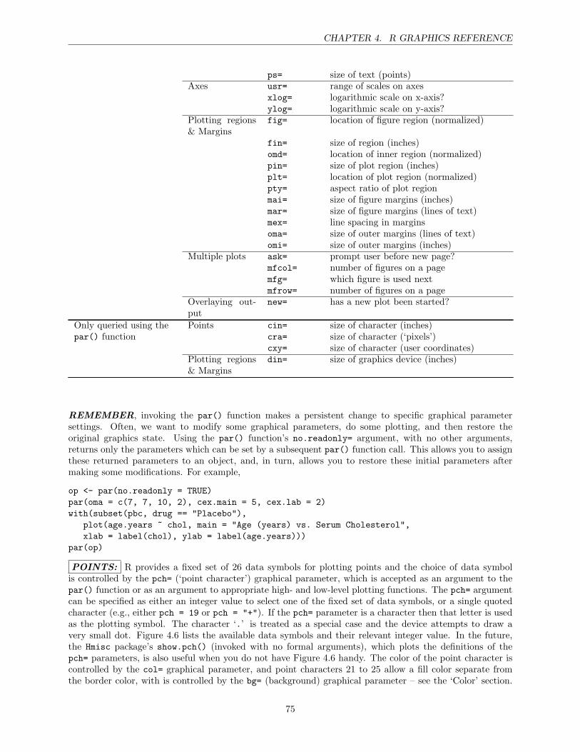
CHAPTER 4. R GRAPHICS REFERENCE
ps= size of text (points)Axes usr= range of scales on axes
xlog= logarithmic scale on x-axis?ylog= logarithmic scale on y-axis?
Plotting regions& Margins
fig= location of figure region (normalized)
fin= size of region (inches)omd= location of inner region (normalized)pin= size of plot region (inches)plt= location of plot region (normalized)pty= aspect ratio of plot regionmai= size of figure margins (inches)mar= size of figure margins (lines of text)mex= line spacing in marginsoma= size of outer margins (lines of text)omi= size of outer margins (inches)
Multiple plots ask= prompt user before new page?mfcol= number of figures on a pagemfg= which figure is used nextmfrow= number of figures on a page
Overlaying out-put
new= has a new plot been started?
Only queried using the Points cin= size of character (inches)par() function cra= size of character (‘pixels’)
cxy= size of character (user coordinates)Plotting regions& Margins
din= size of graphics device (inches)
REMEMBER, invoking the par() function makes a persistent change to specific graphical parametersettings. Often, we want to modify some graphical parameters, do some plotting, and then restore theoriginal graphics state. Using the par() function’s no.readonly= argument, with no other arguments,returns only the parameters which can be set by a subsequent par() function call. This allows you to assignthese returned parameters to an object, and, in turn, allows you to restore these initial parameters aftermaking some modifications. For example,
op <- par(no.readonly = TRUE)par(oma = c(7, 7, 10, 2), cex.main = 5, cex.lab = 2)with(subset(pbc, drug == "Placebo"),
plot(age.years ~ chol, main = "Age (years) vs. Serum Cholesterol",xlab = label(chol), ylab = label(age.years)))
par(op)
POINTS: R provides a fixed set of 26 data symbols for plotting points and the choice of data symbolis controlled by the pch= (‘point character’) graphical parameter, which is accepted as an argument to thepar() function or as an argument to appropriate high- and low-level plotting functions. The pch= argumentcan be specified as either an integer value to select one of the fixed set of data symbols, or a single quotedcharacter (e.g., either pch = 19 or pch = "+"). If the pch= parameter is a character then that letter is usedas the plotting symbol. The character ‘.’ is treated as a special case and the device attempts to draw avery small dot. Figure 4.6 lists the available data symbols and their relevant integer value. In the future,the Hmisc package’s show.pch() (invoked with no formal arguments), which plots the definitions of thepch= parameters, is also useful when you do not have Figure 4.6 handy. The color of the point character iscontrolled by the col= graphical parameter, and point characters 21 to 25 allow a fill color separate fromthe border color, with is controlled by the bg= (background) graphical parameter – see the ‘Color’ section.
75
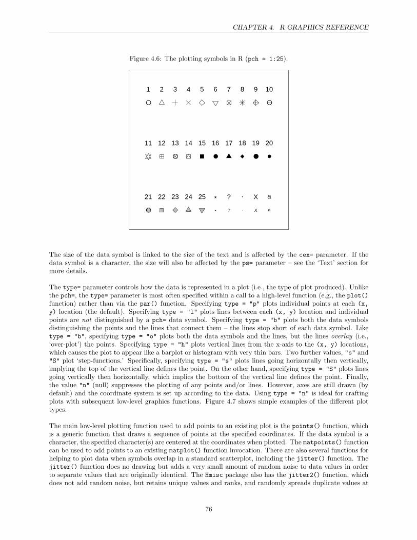
CHAPTER 4. R GRAPHICS REFERENCE
Figure 4.6: The plotting symbols in R (pch = 1:25).
1 2 3 4 5 6 7 8 9 10
11 12 13 14 15 16 17 18 19 20
21 22 23 24 25 * ? . X a
* ? X a
The size of the data symbol is linked to the size of the text and is affected by the cex= parameter. If thedata symbol is a character, the size will also be affected by the ps= parameter – see the ‘Text’ section formore details.
The type= parameter controls how the data is represented in a plot (i.e., the type of plot produced). Unlikethe pch=, the type= parameter is most often specified within a call to a high-level function (e.g., the plot()function) rather than via the par() function. Specifying type = "p" plots individual points at each (x,y) location (the default). Specifying type = "l" plots lines between each (x, y) location and individualpoints are not distinguished by a pch= data symbol. Specifying type = "b" plots both the data symbolsdistinguishing the points and the lines that connect them – the lines stop short of each data symbol. Liketype = "b", specifying type = "o" plots both the data symbols and the lines, but the lines overlay (i.e.,‘over-plot’) the points. Specifying type = "h" plots vertical lines from the x-axis to the (x, y) locations,which causes the plot to appear like a barplot or histogram with very thin bars. Two further values, "s" and"S" plot ‘step-functions.’ Specifically, specifying type = "s" plots lines going horizontally then vertically,implying the top of the vertical line defines the point. On the other hand, specifying type = "S" plots linesgoing vertically then horizontally, which implies the bottom of the vertical line defines the point. Finally,the value "n" (null) suppresses the plotting of any points and/or lines. However, axes are still drawn (bydefault) and the coordinate system is set up according to the data. Using type = "n" is ideal for craftingplots with subsequent low-level graphics functions. Figure 4.7 shows simple examples of the different plottypes.
The main low-level plotting function used to add points to an existing plot is the points() function, whichis a generic function that draws a sequence of points at the specified coordinates. If the data symbol is acharacter, the specified character(s) are centered at the coordinates when plotted. The matpoints() functioncan be used to add points to an existing matplot() function invocation. There are also several functions forhelping to plot data when symbols overlap in a standard scatterplot, including the jitter() function. Thejitter() function does no drawing but adds a very small amount of random noise to data values in orderto separate values that are originally identical. The Hmisc package also has the jitter2() function, whichdoes not add random noise, but retains unique values and ranks, and randomly spreads duplicate values at
76
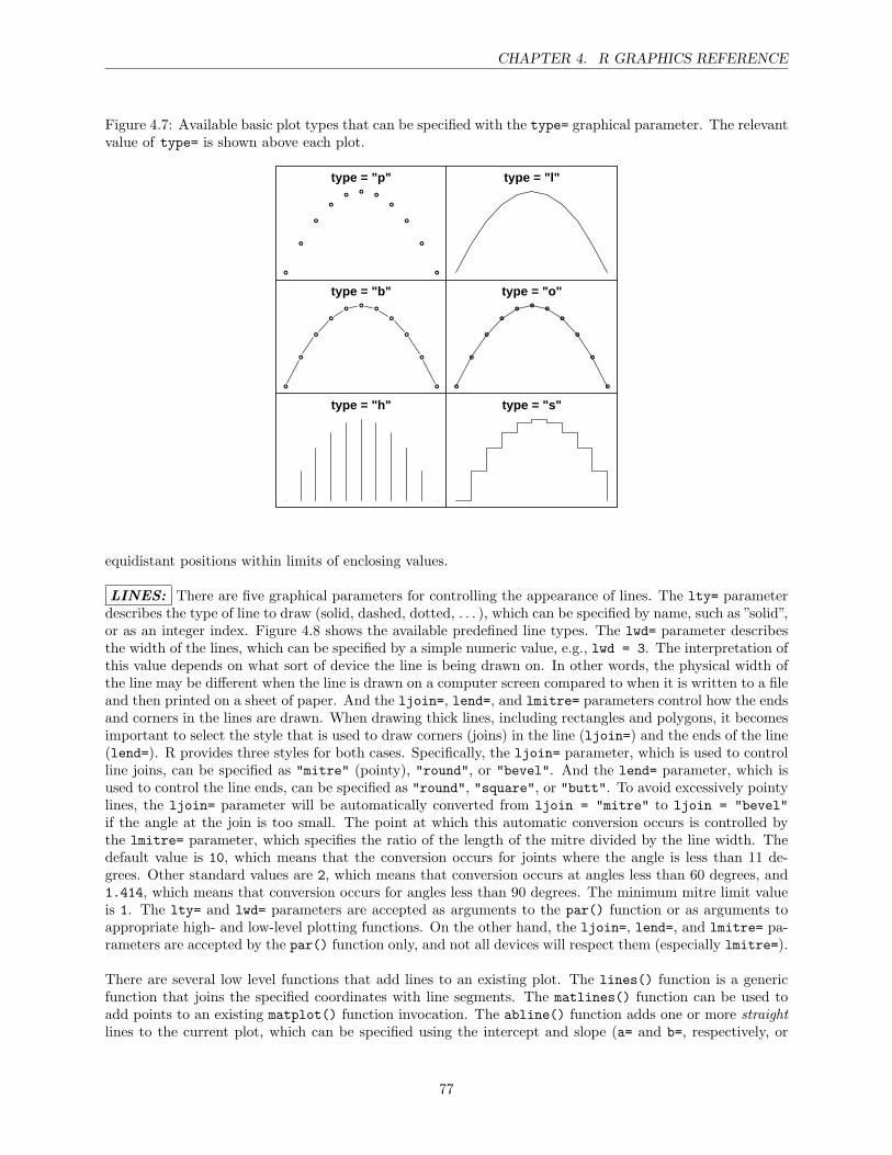
CHAPTER 4. R GRAPHICS REFERENCE
Figure 4.7: Available basic plot types that can be specified with the type= graphical parameter. The relevantvalue of type= is shown above each plot.
x
type = "p"
x
y
type = "l"
x
type = "b"
xy
type = "o"
type = "h"y
type = "s"
equidistant positions within limits of enclosing values.
LINES: There are five graphical parameters for controlling the appearance of lines. The lty= parameterdescribes the type of line to draw (solid, dashed, dotted, . . . ), which can be specified by name, such as ”solid”,or as an integer index. Figure 4.8 shows the available predefined line types. The lwd= parameter describesthe width of the lines, which can be specified by a simple numeric value, e.g., lwd = 3. The interpretation ofthis value depends on what sort of device the line is being drawn on. In other words, the physical width ofthe line may be different when the line is drawn on a computer screen compared to when it is written to a fileand then printed on a sheet of paper. And the ljoin=, lend=, and lmitre= parameters control how the endsand corners in the lines are drawn. When drawing thick lines, including rectangles and polygons, it becomesimportant to select the style that is used to draw corners (joins) in the line (ljoin=) and the ends of the line(lend=). R provides three styles for both cases. Specifically, the ljoin= parameter, which is used to controlline joins, can be specified as "mitre" (pointy), "round", or "bevel". And the lend= parameter, which isused to control the line ends, can be specified as "round", "square", or "butt". To avoid excessively pointylines, the ljoin= parameter will be automatically converted from ljoin = "mitre" to ljoin = "bevel"if the angle at the join is too small. The point at which this automatic conversion occurs is controlled bythe lmitre= parameter, which specifies the ratio of the length of the mitre divided by the line width. Thedefault value is 10, which means that the conversion occurs for joints where the angle is less than 11 de-grees. Other standard values are 2, which means that conversion occurs at angles less than 60 degrees, and1.414, which means that conversion occurs for angles less than 90 degrees. The minimum mitre limit valueis 1. The lty= and lwd= parameters are accepted as arguments to the par() function or as arguments toappropriate high- and low-level plotting functions. On the other hand, the ljoin=, lend=, and lmitre= pa-rameters are accepted by the par() function only, and not all devices will respect them (especially lmitre=).
There are several low level functions that add lines to an existing plot. The lines() function is a genericfunction that joins the specified coordinates with line segments. The matlines() function can be used toadd points to an existing matplot() function invocation. The abline() function adds one or more straightlines to the current plot, which can be specified using the intercept and slope (a= and b=, respectively, or
77
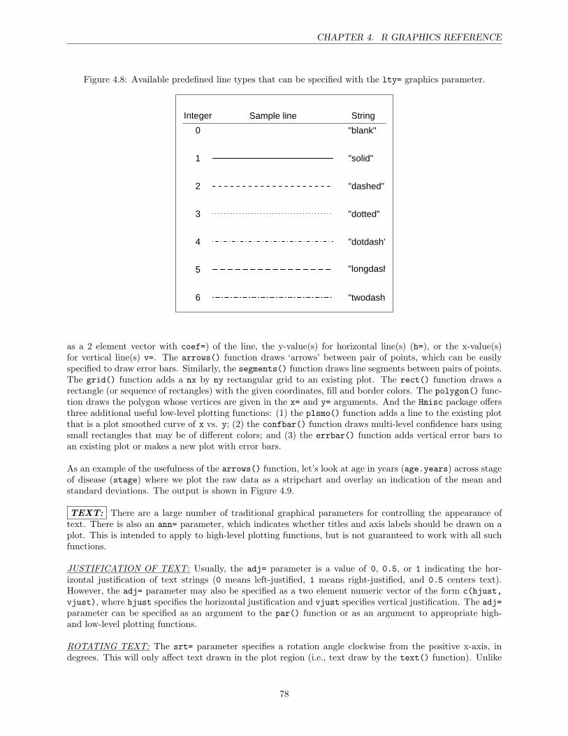
CHAPTER 4. R GRAPHICS REFERENCE
Figure 4.8: Available predefined line types that can be specified with the lty= graphics parameter.
0
1
2
3
4
5
6
"blank"
"solid"
"dashed"
"dotted"
"dotdash"
"longdash"
"twodash"
Integer Sample line String
as a 2 element vector with coef=) of the line, the y-value(s) for horizontal line(s) (h=), or the x-value(s)for vertical line(s) v=. The arrows() function draws ‘arrows’ between pair of points, which can be easilyspecified to draw error bars. Similarly, the segments() function draws line segments between pairs of points.The grid() function adds a nx by ny rectangular grid to an existing plot. The rect() function draws arectangle (or sequence of rectangles) with the given coordinates, fill and border colors. The polygon() func-tion draws the polygon whose vertices are given in the x= and y= arguments. And the Hmisc package offersthree additional useful low-level plotting functions: (1) the plsmo() function adds a line to the existing plotthat is a plot smoothed curve of x vs. y; (2) the confbar() function draws multi-level confidence bars usingsmall rectangles that may be of different colors; and (3) the errbar() function adds vertical error bars toan existing plot or makes a new plot with error bars.
As an example of the usefulness of the arrows() function, let’s look at age in years (age.years) across stageof disease (stage) where we plot the raw data as a stripchart and overlay an indication of the mean andstandard deviations. The output is shown in Figure 4.9.
TEXT: There are a large number of traditional graphical parameters for controlling the appearance oftext. There is also an ann= parameter, which indicates whether titles and axis labels should be drawn on aplot. This is intended to apply to high-level plotting functions, but is not guaranteed to work with all suchfunctions.
JUSTIFICATION OF TEXT: Usually, the adj= parameter is a value of 0, 0.5, or 1 indicating the hor-izontal justification of text strings (0 means left-justified, 1 means right-justified, and 0.5 centers text).However, the adj= parameter may also be specified as a two element numeric vector of the form c(hjust,vjust), where hjust specifies the horizontal justification and vjust specifies vertical justification. The adj=parameter can be specified as an argument to the par() function or as an argument to appropriate high-and low-level plotting functions.
ROTATING TEXT: The srt= parameter specifies a rotation angle clockwise from the positive x-axis, indegrees. This will only affect text drawn in the plot region (i.e., text draw by the text() function). Unlike
78
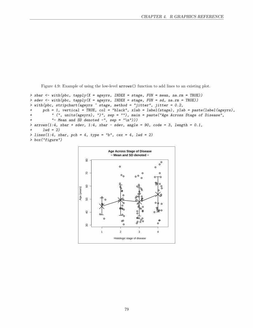
CHAPTER 4. R GRAPHICS REFERENCE
Figure 4.9: Example of using the low-level arrows() function to add lines to an existing plot.
> xbar <- with(pbc, tapply(X = ageyrs, INDEX = stage, FUN = mean, na.rm = TRUE))
> sdev <- with(pbc, tapply(X = ageyrs, INDEX = stage, FUN = sd, na.rm = TRUE))
> with(pbc, stripchart(ageyrs ~ stage, method = "jitter", jitter = 0.2,
+ pch = 1, vertical = TRUE, col = "black", xlab = label(stage), ylab = paste(label(ageyrs),
+ " (", units(ageyrs), ")", sep = ""), main = paste("Age Across Stage of Disease",
+ "- Mean and SD denoted -", sep = "\n")))
> arrows(1:4, xbar + sdev, 1:4, xbar - sdev, angle = 90, code = 3, length = 0.1,
+ lwd = 2)
> lines(1:4, xbar, pch = 4, type = "b", cex = 4, lwd = 2)
> box("figure")
1 2 3 4
3040
5060
7080
Age Across Stage of Disease− Mean and SD denoted −
Histologic stage of disease
Age
(ye
ars)
79
CHAPTER 4. R GRAPHICS REFERENCE
within the plot region, in the figure and outer margins, text may only be drawn at angles that are multiplesof 90 degrees, and this angle is controlled by the las= parameter. A value of 0 means that text is alwaysdrawn parallel to the relevant axis (i.e., horizontal in margins 1 and 3, and vertical in margins 2 and 4). Avalue of 1 means text is always horizontal, 2 means text is always perpendicular to the relevant axis, and3 means text is always vertical. This parameter interacts with or overrides the adj= and srt= parameters.Both the srt= and las= parameters can be specified as an argument to the par() function or as an argumentto appropriate high- and low-level plotting functions.
TEXT SIZE: The size of text is ultimately a numerical value specifying the size of the font in ‘points.’The font size is controlled by two parameters: the ps= parameter specifies an absolute font size parameter(e.g., ps = 9; can only be set via the par() function), and the cex= parameter specifies a multiplicativemagnification modifier (e.g., cex = 1.5; a value < 1 shrinks the text and a value > 1 enlarges text). Aswith specifying color, the scope of a cex= parameter can vary depending on where it is given. When cex=is specified via the par() function, it affects most text. However, when cex= is specified via the plot()function, it only affects the size of the data symbols. Luckily, there are special parameters for controlling thesize of text that is drawn as axis tick labels (cex.axis=), text that is drawn as axis labels (cex.lab=), textin the title (cex.main=), and text in the sub-title (cex.sub=). These four arguments can also be used asarguments in most high-level plotting functions. There is also a tmag= parameter for controlling the amountto magnify title text relative to other plot labels, which can also be used as an argument in most high-levelplotting functions. Finally, the strheight() and strwidth() functions can be used to compute the heightor width of character strings or mathematical expression, respectively, on the current plotting device in usercoordinates, inches, or as fraction of the figure width.
MULTI-LINE TEXT: It is possible to draw text that spans several lines by inserting a new line escapesequence, "\n", within a piece of text. For example, "first line\nsecond line". The spacing betweenlines is controlled by the lheight= parameter, which is a multiplier added to the natural height of a line oftext (e.g., lheight = 2 specifies double-space text), and can only be specified via the par() function.
SPECIFYING FONTS: The font face is specified via the font= parameter as an integer, and can be spec-ified as an argument to the par() function or as an argument to appropriate high- and low-level plottingfunctions. font = 1 produces Roman or upright face; font = 2 produces bold face font; font = 3 producesslanted or italic face; and font = 4 produces bold and slanted face. As with color and text size, the font=parameter applies only to text drawn in the plot region. There are also additional parameters specifically foraxes (font.axis=), labels (font.lab=), and titles (font.main= and font.sub=). These four arguments canalso be used as arguments in most high-level plotting functions. Also, every graphics device establishes adefault font family, which is usually a sans serif font such as Helvetica or Arial. A new font family is specifiedusing the family= parameter via the par() function.
In addition to all of these graphical parameters, there are a large number of low-level plotting functions thatcontrol the placement of text onto your plot. For instance, the text() function draws the supplied textstrings at specified coordinates within the plot region. The mtext() function writes text in one of the fourmargins of the current figure region or one of the four outer margins of the device region – see the ‘Plottingregions & Margins’ section for more details. And the title() function can be used to add labels to a plot– the main plot title (the main= argument; placed at top), the plot sub-title (the sub= argument; placedat bottom), the x-axis label (the xlab= argument), and the y-axis label (the ylab= argument). These fourarguments can also be used as arguments in most high-level plotting functions.
There is also the identify() function, which can be used to interactively add labels to data symbols on aplot. The identify() function performs no plotting itself, but simply allows the user to move the mousepointer and click the left mouse buttton near a point. If there is a point near the mouse pointer it will bemarked with its index number (that is, its position in the x/y vectors) plotted nearby. Alternatively, youcould use some informative string (such as a case name) as a highlight by using the identify() function’slabels= argument, or disable marking altogether with the plot = FALSE argument. When the process isterminated, the identify() function returns the indices of the selected points; you can use these indices to
80
CHAPTER 4. R GRAPHICS REFERENCE
extract the selected points from the original vectors x and y.
COLOR: There are three main color parameters: col=, fg=, and bg=. The col= parameter is the mostcommonly used. The primary use is to specify the color of points, lines, text, and so on that are drawn in theplot region. Unfortunately, when specified via a high- and/or low-level plotting function, the effect can vary.For example, a standard scatterplot produced by the high-level plot() function will use the col= parameterfor coloring data symbols and lines, but the high-level barplot() function will use the col= parameter forfilling the contents of its bars. In the low-level rect() function, the col= parameter provides the color tofill the rectangle and there is a border= argument specific to the low-level rect() function that gives thecolor to draw the border of the rectangle. The effect of the col= parameter on graphical output drawn inthe margins also varies. It does not affect the color of axes and axis labels, but it does affect the output fromthe low-level mtext() function. There are also specific parameters for affecting axes, labels, titles, and sub-titles called col.axis=, col.lab=, col.main=, and col.sub=, respectively. The fg= parameter is primarilyintended for specifying the color of axes and borders on plots. There is some overlap between this and thespecific col.axis=, col.main=, etc parameters mentioned above. The bg= parameter is primarily intendedto specify the color of the background for graphical output. This color is used to fill the entire page. Aswith the col= parameter, when bg= is specified in a graphics function it can have a quite different meaning.For example, the high-level plot() function and the low-level points() function use the bg= parameterto specify the color for the interior of the points, which can have different colors on the border (i.e., pch=parameter values 21 to 25; see the ‘Points’ section). There is also the gamma= parameter that controls thegamma correction for a device. On most devices this can only be set once the device is first opened.
SPECIFYING COLOR: The easiest way to specify a color in R is simply to use the color’s name. Forexample, "red" can be used to specify that graphical output should be (a very bright) red. R understandsa fairly large set of color names (657 to be exact), which can be returned by the colors() (or colours())functions (invoked with no formal arguments). The following function generates a matrix of rectangles thatdisplays the corresponding color of each of the 657 possible colors you can specify with the colors() function.
show.colors <- function(x = 22,y = 30)par(mar = c(0.1, 0.1, 0.1, 0.1))plot(c( -1, x), c(-1, y), xlab = "", ylab = "", type = "n", xaxt = "n", yaxt = "n", bty = "n")for(i in 1:x)
for(j in 1:y)k <- y*(i - 1) + j ; co <- colors()[k]rect(i - 1, j - 1, i, j, col = co, border = 1)
text(rep(-0.5, y), (1:y) - 0.5, 1:y, cex = 1.2 - 0.016*y)text((1:x) - 0.5, rep(-0.5, x), y*(0:(x-1)), cex = 1.2 - 0.022*x)
show.colors()
By default, R has a color palette of eight colors, which can be returned by the palette() function (invokedwith no formal arguments):
> palette()
[1] "black" "red" "green3" "blue" "cyan" "magenta" "yellow" "gray"
In addition to being able to specify these eight colors by name, these eight colors can also be specified byinteger values (i.e. 1 through 8). The Hmisc package’s show.col() function plots the definitions of theseeight integer-value colors in case you forget. It is also possible to specify the colors using one of the standardcolor-space descriptions. For example, the rgb() function allows a color to be specified as a Red-Green-Blue(RGB) triplet of intensities. For example, using this function, the color red is specified as rgb(1, 0, 0)(i.e., as much red as possible, no blue, and no green). The col2rgb() function can be used to see the RGBvalues for a particular color name. An alternative way to provide an RGB color specification is to provide astring of the form "#RRGGBB", where each of the pair RR, GG, and BB consist of two hexadecimal digits givinga value in the range zero (00) to 255 (FF). In this specification, the color red is given as "#FF0000". There
81

CHAPTER 4. R GRAPHICS REFERENCE
is also an hsv() function for specifying a color as a Hue-Saturation-Value (HSV) triplet. The terminologyof color spaces is fraught, but roughly speaking: hue corresponds to a position of the rainbow, from red(0), through orange, yellow, green, blue, indigo, to violet (1); saturation determines whether the color isdull or bright; and value determines whether the color is light or dark. The HSV specification for the (verybright) color red is hsv(0, 1, 1). The rgb2hsv() function converts a color specification from RGB to HSV.
COLOR SETS: More than one color is often required within a single plot and in such cases it can be difficultto select colors that are aesthetically pleasing or are related in some way (e.g., a set of color in which thebrightness of the colors decreases in regular steps). The following table lists some functions that R providesfor generating sets of colors. Each of the functions listed selects a set of colors by taking regular steps alonga path through the HSV color space. Also, the colorRamp() and colorRampPalette() functions can beused to interpolate a new color set from an existing set of colors.
Name Descriptionrainbow() Colors vary from red through orange, yellow, green, blue, and indigo, to violet.heat.colors() Colors vary from white, through orange, to red.terrain.colors() Colors vary from white, through brown, to green.topo.colors() Colors vary from white, through brown then green, to blue.cm.colors() Colors vary from light blue, through white, to light magenta.gray() A set of shades of gray.gray.colors() A set of gamma-corrected gray colors.
AXES: By default, the traditional graphics system produces axes with sensible labels and tick marks atsensible locations. However, if the axis does not look right, there are a number of graphical parametersspecifically for controlling aspects such as the number of tick marks and the positioning of labels. Recall,most high-level plotting functions provide xlim= and ylim= arguments to control the range of the scale onthe axes. If none of these gives the desired result, you may have to resort to drawing the axis explicitly usingthe low-level axis() plotting function – more to come.
The lab= parameter in the traditional graphics state is used to control the number of tick marks on theaxes. The parameter is only used as a starting point for the algorithm R uses to determine sensible tickmark locations so the final number of tick marks that are drawn could easily differ from this specification.The parameter takes two values: the first specifies the number of tick marks on the x-axis and the secondspecifies the number of tick marks on the y-axis.
The xaxp= and yaxp= parameter also relate to the number and location of the tick marks on the axes ofa plot. This parameter is almost always calculated by R for each new plot so user parameters are usuallyoverridden. In other words, it only makes sense to query this parameter for its current value. The parametersconsist of three values: the first two specify the location of the left-most and right-most tick-marks (bottomand top tick-marks for the y-axis), and the third value specifies how many intervals there are between tickmarks. However, when a log transformation is in effect for an axis, the three values have a different meaningaltogether (see the par() function’s help file).
The mgp= parameter controls the distance that the components of the axes are drawn away from the edge ofthe plot region. There are three values representing (in order) the positioning of the axis label, the tick marklabels, and the axis line. The values are in terms of lines of text away from the edges of the plot region. Bydefault mgp = c(3, 1, 0).
The tck= and tcl= parameters control the length of the tick marks. The tcl= parameter specifies the lengthof tick marks as a fraction of the height of a line of text. The sign dictates the direction of the tick marks – anegative value draws tick marks outside the plot region and a positive value draws tick marks inside the plot
82
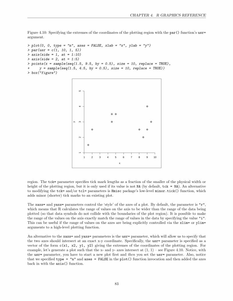
CHAPTER 4. R GRAPHICS REFERENCE
Figure 4.10: Specifying the extremes of the coordinates of the plotting region with the par() function’s usr=argument.
> plot(0, 0, type = "n", axes = FALSE, xlab = "x", ylab = "y")
> par(usr = c(1, 10, 1, 5))
> axis(side = 1, at = 1:10)
> axis(side = 2, at = 1:5)
> points(x = sample(seq(1.5, 9.5, by = 0.5), size = 10, replace = TRUE),
+ y = sample(seq(1.5, 4.5, by = 0.5), size = 10, replace = TRUE))
> box("figure")
x
y
1 2 3 4 5 6 7 8 9 10
12
34
5
region. The tck= parameter specifies tick mark lengths as a fraction of the smaller of the physical width orheight of the plotting region, but it is only used if its value is not NA (by default, tck = NA). An alternativeto modifying the tck= and/or tcl= parameters is Hmisc package’s low-level minor.tick() function, whichadds minor (shorter) tick marks to an existing plot.
The xaxs= and yaxs= parameters control the ‘style’ of the axes of a plot. By default, the parameter is "r",which means that R calculates the range of values on the axis to be wider than the range of the data beingplotted (so that data symbols do not collide with the boundaries of the plot region). It is possible to makethe range of the values on the axis exactly match the range of values in the data by specifying the value "i".This can be useful if the range of values on the axes are being explicitly controlled via the xlim= or ylim=arguments to a high-level plotting function.
An alternative to the xaxs= and yaxs= parameters is the usr= parameter, which will allow us to specify thatthe two axes should intersect at an exact x-y coordinate. Specifically, the usr= parameter is specified as avector of the form c(x1, x2, y1, y2) giving the extremes of the coordinates of the plotting region. Forexample, let’s generate a plot such that the x- and y- axes intersect at (1, 1) – see Figure 4.10. Notice, withthe usr= parameter, you have to start a new plot first and then you set the usr= parameter. Also, noticethat we specified type = "n" and axes = FALSE in the plot() function invocation and then added the axesback in with the axis() function.
83
CHAPTER 4. R GRAPHICS REFERENCE
The xaxt= and yaxt= parameters control the ‘type’ of axes. The default value, "s", means that the axis isdrawn. Specifying a value of "n" means that the axis is not drawn.
The xlog= and ylog= parameters control the transformations of the values on the axes. The default valueis FALSE, which means that the axes are linear and values are not transformed. If this value is TRUE then alogarithmic transformation is applied to any values on the relevant dimension in the plot region. This alsoaffects the calculation of tick mark locations on the axes.
The bty= parameter is not strictly to do with axes, but it controls the type of ‘box’ that is drawn around aplot. The value can be "n", which means that no box is drawn, or it can be one of "o", "l", "7", "c", "u",or "]", which means that the box drawn resembles the corresponding uppercase character. For example, bty= "c" means that the bottom, left, and top borders will be draw, but the right border will not be drawn. Analternative to using the bty= parameter is to use the low-level box() function. With the box() function youcan specify the box-type (bty=), color (col=), line type (lty=), and line width (lwd=) of the box drawn. Youcan also specify which (which=) box to draw. By default, the box() function will draw a box connecting allfour axes (which = "plot"). However, which= can be changed to "figure", "inner", or "outer", whichcome in very handy when you want to outline the wholeplot or specific plots when plotting multiple plots.
In some case, it may be useful to draw tick marks at the locations that the default axis would use, but withdifferent labels. The axTicks() function can be used to calculate these default locations. This function isalso useful for enforcing an xaxp= (or yaxp=) graphical parameter. If these parameters are specified via thepar() function, they usually have no effect because the traditional graphics system almost always calculatesthe parameter itself. You can choose these parameters by passing them as arguments to the axTicks() func-tion and then passing the resulting locations via the at= argument to the axis() function. The pretty()function is another useful function for determining where to place the tick marks.
THE axis() FUNCTION: When using the axis() function to draw an axis ‘from scratch,’ the first stepis to inhibit the default axes. Most high-level plotting functions should provide an axes= argument which,when set to FALSE, indicates that the axes should not be drawn. Specifying the graphical parameter xaxt= "n" (or yaxt = "n") or ann = FALSE via the par() function may also do the trick. Once this is done,the axis() function can draw axes on any side of the plot (specified by the side= argument), and youcan specify the location along the axis of tick marks and the text to use for tick labels using the at= andlabels= arguments, respectively. See Figure 4.11 for an example. The axis() function is not generic, butthere are special alternative functions for plotting time related data. Specifically, the axis.Date() andaxis.POSIXct() functions take an object containing dates and produce an axis with appropriate labelsrepresenting times, days, months, and years (e.g., 10:15, Jan 12, or 1995). In addition, the axis() func-tion is useful to superimpose the underlying numerical axes that are used by functions like dotchart(),stripchart(), boxplot(), or barplot() – use axis(side = 1) to superimpose the x-axis and axis(side= 2) for the y-axis. This allows you to determine the x-y location of specific things in the plot, such aswhere to place a legend or the middle of a bar in order to add text. Lastly, the axis() function canbe used to draw text in the margins – see Figure 4.12 for an example.1 It is important to realize thatthe axis() function will not allow you to place any text in the margin areas where two axes intersect. Analternative is to use the mtext() function (discussed in the ‘Text’ section) with its line= and at= arguments.
PLOTTING REGIONS & MARGINS: In the base graphics system, every page is split up into threemain regions: (1) the outer margins; (2) the current figure region; and (3) the current plot region. Figure4.13 shows these regions when there is only one figure on the page and Figure 4.14 shows the regions whenthere are multiple figures on the page. The region obtained by removing the outer margins from the deviceis called the inner region. When there is only one figure, this usually corresponds to the figure region, butwhen there are multiple figures the inner region corresponds to the union of all figure regions. The areaoutside the plot region, but inside the figure region is referred to as the figure margins. A typical high-levelfunction draws data symbols and lines within the plot region and axes and labels in the figure or outer
1The rates.dat file contains a data set for a study of beta-blocker adherence post-AMI.
84
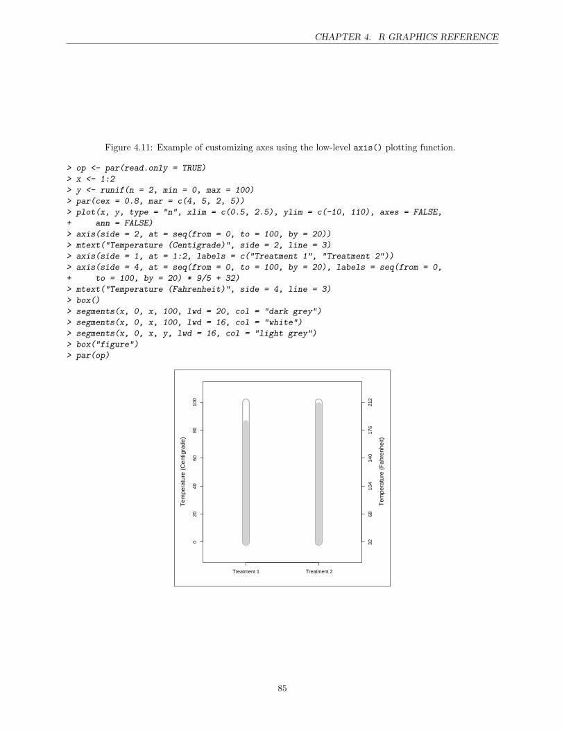
CHAPTER 4. R GRAPHICS REFERENCE
Figure 4.11: Example of customizing axes using the low-level axis() plotting function.
> op <- par(read.only = TRUE)
> x <- 1:2
> y <- runif(n = 2, min = 0, max = 100)
> par(cex = 0.8, mar = c(4, 5, 2, 5))
> plot(x, y, type = "n", xlim = c(0.5, 2.5), ylim = c(-10, 110), axes = FALSE,
+ ann = FALSE)
> axis(side = 2, at = seq(from = 0, to = 100, by = 20))
> mtext("Temperature (Centigrade)", side = 2, line = 3)
> axis(side = 1, at = 1:2, labels = c("Treatment 1", "Treatment 2"))
> axis(side = 4, at = seq(from = 0, to = 100, by = 20), labels = seq(from = 0,
+ to = 100, by = 20) * 9/5 + 32)
> mtext("Temperature (Fahrenheit)", side = 4, line = 3)
> box()
> segments(x, 0, x, 100, lwd = 20, col = "dark grey")
> segments(x, 0, x, 100, lwd = 16, col = "white")
> segments(x, 0, x, y, lwd = 16, col = "light grey")
> box("figure")
> par(op)
020
4060
8010
0
Tem
pera
ture
(C
entig
rade
)
Treatment 1 Treatment 2
3268
104
140
176
212
Tem
pera
ture
(F
ahre
nhei
t)
85
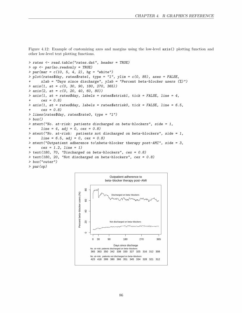
CHAPTER 4. R GRAPHICS REFERENCE
Figure 4.12: Example of customizing axes and margins using the low-level axis() plotting function andother low-level text plotting functions.
> rates <- read.table("rates.dat", header = TRUE)
> op <- par(no.readonly = TRUE)
> par(mar = c(10, 5, 4, 2), bg = "white")
> plot(rates$day, rates$rate1, type = "l", ylim = c(0, 85), axes = FALSE,
+ xlab = "Days since discharge", ylab = "Percent beta-blocker users (%)")
> axis(1, at = c(0, 30, 90, 180, 270, 365))
> axis(2, at = c(0, 20, 40, 60, 80))
> axis(1, at = rates$day, labels = rates$atrisk1, tick = FALSE, line = 4,
+ cex = 0.8)
> axis(1, at = rates$day, labels = rates$atrisk0, tick = FALSE, line = 6.5,
+ cex = 0.8)
> lines(rates$day, rates$rate0, type = "l")
> box()
> mtext("No. at-risk: patients discharged on beta-blockers", side = 1,
+ line = 4, adj = 0, cex = 0.8)
> mtext("No. at-risk: patients not discharged on beta-blockers", side = 1,
+ line = 6.5, adj = 0, cex = 0.8)
> mtext("Outpatient adherence to\nbeta-blocker therapy post-AMI", side = 3,
+ cex = 1.2, line = 1)
> text(180, 70, "Discharged on beta-blockers", cex = 0.8)
> text(180, 20, "Not discharged on beta-blockers", cex = 0.8)
> box("outer")
> par(op)
Days since discharge
Per
cent
bet
a−bl
ocke
r us
ers
(%)
0 30 90 180 270 365
020
4060
80
365 363 350 342 338 330 327 325 316 312 308
423 418 399 380 366 351 345 334 328 321 312
No. at−risk: patients discharged on beta−blockers
No. at−risk: patients not discharged on beta−blockers
Outpatient adherence tobeta−blocker therapy post−AMI
Discharged on beta−blockers
Not discharged on beta−blockers
86
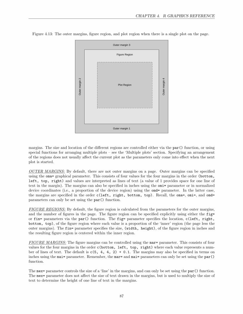
CHAPTER 4. R GRAPHICS REFERENCE
Figure 4.13: The outer margins, figure region, and plot region when there is a single plot on the page.
Plot Region
Figure Region
Outer margin 1
Out
er m
argi
n 2
Outer margin 3
Out
er m
argi
n 4
margins. The size and location of the different regions are controlled either via the par() function, or usingspecial functions for arranging multiple plots – see the ‘Multiple plots’ section. Specifying an arrangementof the regions does not usually affect the current plot as the parameters only come into effect when the nextplot is started.
OUTER MARGINS: By default, there are not outer margins on a page. Outer margins can be specifiedusing the oma= graphical parameter. This consists of four values for the four margins in the order (bottom,left, top, right) and values are interpreted as lines of text (a value of 1 provides space for one line oftext in the margin). The margins can also be specified in inches using the omi= parameter or in normalizeddevice coordinates (i.e., a proportion of the device region) using the omd= parameter. In the latter case,the margins are specified in the order c(left, right, bottom, top). Recall, the oma=, omi=, and omd=parameters can only be set using the par() function.
FIGURE REGIONS: By default, the figure region is calculated from the parameters for the outer margins,and the number of figures in the page. The figure region can be specified explicitly using either the fig=or fin= parameters via the par() function. The fig= parameter specifies the location, c(left, right,bottom, top), of the figure region where each value is a proportion of the ‘inner’ region (the page less theouter margins). The fin= parameter specifies the size, (width, height), of the figure region in inches andthe resulting figure region is centered within the inner region.
FIGURE MARGINS: The figure margins can be controlled using the mar= parameter. This consists of fourvalues for the four margins in the order c(bottom, left, top, right) where each value represents a num-ber of lines of text. The default is c(5, 4, 4, 2) + 0.1. The margins may also be specified in terms oninches using the mai= parameter. Remember, the mar= and mai= parameters can only be set using the par()function.
The mex= parameter controls the size of a ‘line’ in the margins, and can only be set using the par() function.The mex= parameter does not affect the size of text drawn in the margins, but is used to multiply the size oftext to determine the height of one line of text in the margins.
87
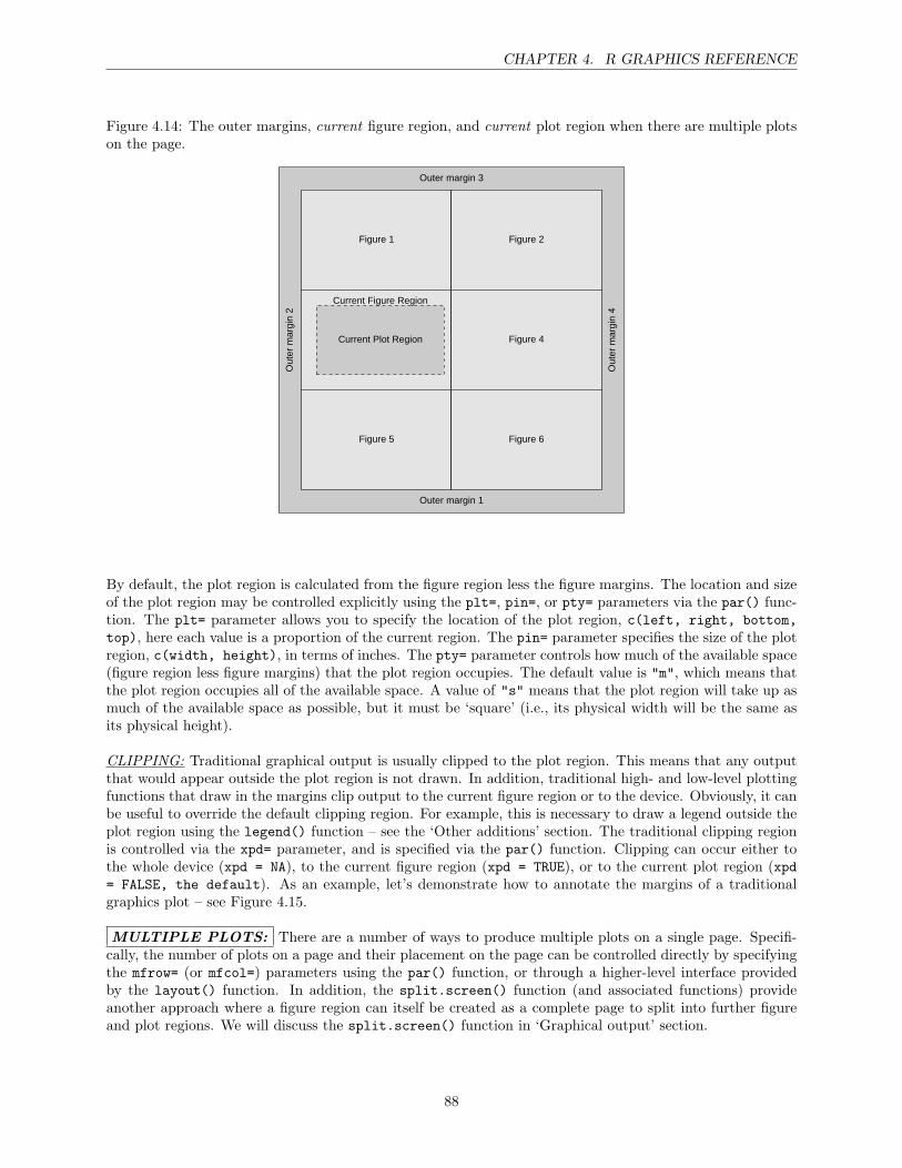
CHAPTER 4. R GRAPHICS REFERENCE
Figure 4.14: The outer margins, current figure region, and current plot region when there are multiple plotson the page.
Figure 1 Figure 2
Current Plot Region
Current Figure Region
Figure 4
Figure 5 Figure 6
Outer margin 1
Out
er m
argi
n 2
Outer margin 3
Out
er m
argi
n 4
By default, the plot region is calculated from the figure region less the figure margins. The location and sizeof the plot region may be controlled explicitly using the plt=, pin=, or pty= parameters via the par() func-tion. The plt= parameter allows you to specify the location of the plot region, c(left, right, bottom,top), here each value is a proportion of the current region. The pin= parameter specifies the size of the plotregion, c(width, height), in terms of inches. The pty= parameter controls how much of the available space(figure region less figure margins) that the plot region occupies. The default value is "m", which means thatthe plot region occupies all of the available space. A value of "s" means that the plot region will take up asmuch of the available space as possible, but it must be ‘square’ (i.e., its physical width will be the same asits physical height).
CLIPPING: Traditional graphical output is usually clipped to the plot region. This means that any outputthat would appear outside the plot region is not drawn. In addition, traditional high- and low-level plottingfunctions that draw in the margins clip output to the current figure region or to the device. Obviously, it canbe useful to override the default clipping region. For example, this is necessary to draw a legend outside theplot region using the legend() function – see the ‘Other additions’ section. The traditional clipping regionis controlled via the xpd= parameter, and is specified via the par() function. Clipping can occur either tothe whole device (xpd = NA), to the current figure region (xpd = TRUE), or to the current plot region (xpd= FALSE, the default). As an example, let’s demonstrate how to annotate the margins of a traditionalgraphics plot – see Figure 4.15.
MULTIPLE PLOTS: There are a number of ways to produce multiple plots on a single page. Specifi-cally, the number of plots on a page and their placement on the page can be controlled directly by specifyingthe mfrow= (or mfcol=) parameters using the par() function, or through a higher-level interface providedby the layout() function. In addition, the split.screen() function (and associated functions) provideanother approach where a figure region can itself be created as a complete page to split into further figureand plot regions. We will discuss the split.screen() function in ‘Graphical output’ section.
88
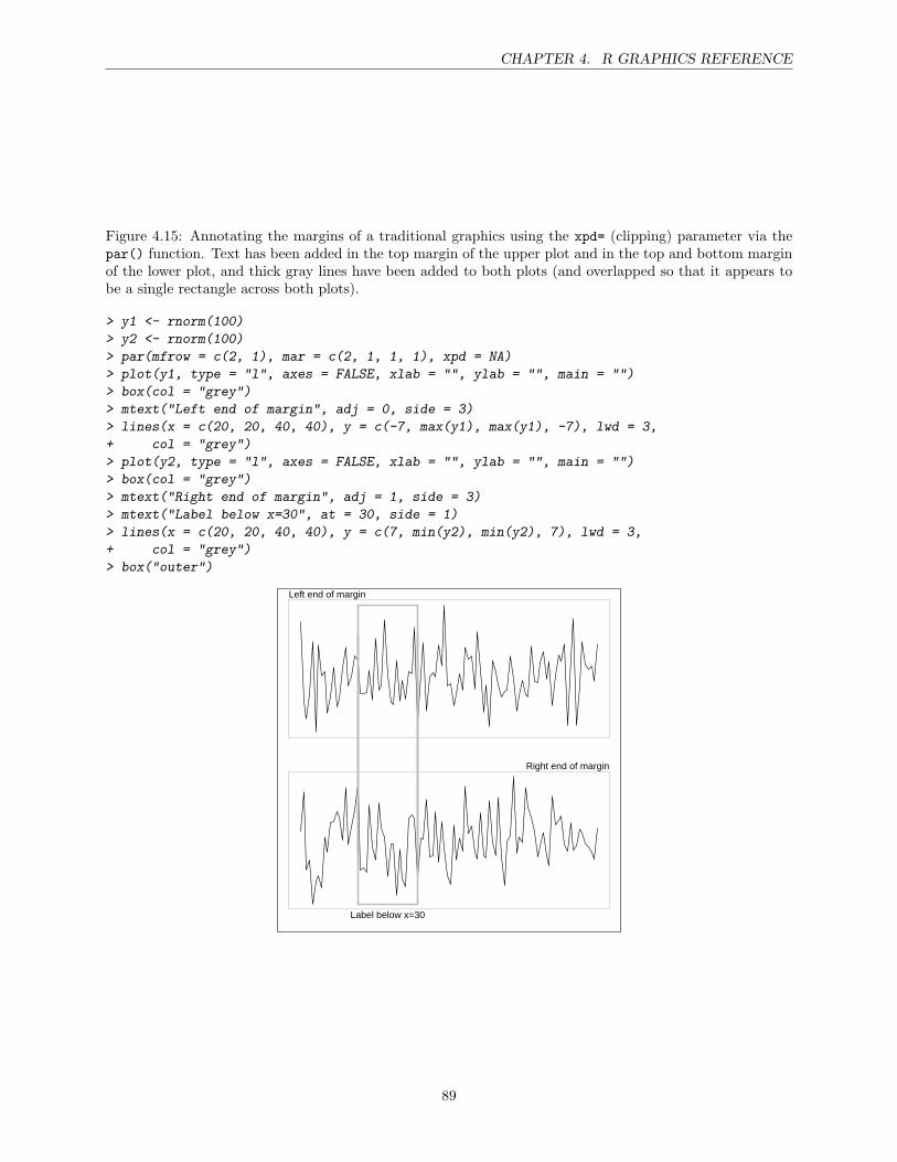
CHAPTER 4. R GRAPHICS REFERENCE
Figure 4.15: Annotating the margins of a traditional graphics using the xpd= (clipping) parameter via thepar() function. Text has been added in the top margin of the upper plot and in the top and bottom marginof the lower plot, and thick gray lines have been added to both plots (and overlapped so that it appears tobe a single rectangle across both plots).
> y1 <- rnorm(100)
> y2 <- rnorm(100)
> par(mfrow = c(2, 1), mar = c(2, 1, 1, 1), xpd = NA)
> plot(y1, type = "l", axes = FALSE, xlab = "", ylab = "", main = "")
> box(col = "grey")
> mtext("Left end of margin", adj = 0, side = 3)
> lines(x = c(20, 20, 40, 40), y = c(-7, max(y1), max(y1), -7), lwd = 3,
+ col = "grey")
> plot(y2, type = "l", axes = FALSE, xlab = "", ylab = "", main = "")
> box(col = "grey")
> mtext("Right end of margin", adj = 1, side = 3)
> mtext("Label below x=30", at = 30, side = 1)
> lines(x = c(20, 20, 40, 40), y = c(7, min(y2), min(y2), 7), lwd = 3,
+ col = "grey")
> box("outer")
Left end of margin
Right end of margin
Label below x=30
89
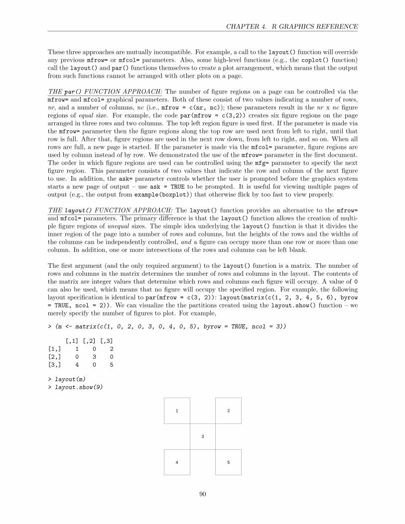
CHAPTER 4. R GRAPHICS REFERENCE
These three approaches are mutually incompatible. For example, a call to the layout() function will overrideany previous mfrow= or mfcol= parameters. Also, some high-level functions (e.g., the coplot() function)call the layout() and par() functions themselves to create a plot arrangement, which means that the outputfrom such functions cannot be arranged with other plots on a page.
THE par() FUNCTION APPROACH: The number of figure regions on a page can be controlled via themfrow= and mfcol= graphical parameters. Both of these consist of two values indicating a number of rows,nr, and a number of columns, nc (i.e., mfrow = c(nr, nc)); these parameters result in the nr x nc figureregions of equal size. For example, the code par(mfrow = c(3,2)) creates six figure regions on the pagearranged in three rows and two columns. The top left region figure is used first. If the parameter is made viathe mfrow= parameter then the figure regions along the top row are used next from left to right, until thatrow is full. After that, figure regions are used in the next row down, from left to right, and so on. When allrows are full, a new page is started. If the parameter is made via the mfcol= parameter, figure regions areused by column instead of by row. We demonstrated the use of the mfrow= parameter in the first document.The order in which figure regions are used can be controlled using the mfg= parameter to specify the nextfigure region. This parameter consists of two values that indicate the row and column of the next figureto use. In addition, the ask= parameter controls whether the user is prompted before the graphics systemstarts a new page of output – use ask = TRUE to be prompted. It is useful for viewing multiple pages ofoutput (e.g., the output from example(boxplot)) that otherwise flick by too fast to view properly.
THE layout() FUNCTION APPROACH: The layout() function provides an alternative to the mfrow=and mfcol= parameters. The primary difference is that the layout() function allows the creation of multi-ple figure regions of unequal sizes. The simple idea underlying the layout() function is that it divides theinner region of the page into a number of rows and columns, but the heights of the rows and the widths ofthe columns can be independently controlled, and a figure can occupy more than one row or more than onecolumn. In addition, one or more intersections of the rows and columns can be left blank.
The first argument (and the only required argument) to the layout() function is a matrix. The number ofrows and columns in the matrix determines the number of rows and columns in the layout. The contents ofthe matrix are integer values that determine which rows and columns each figure will occupy. A value of 0can also be used, which means that no figure will occupy the specified region. For example, the followinglayout specification is identical to par(mfrow = c(3, 2)): layout(matrix(c(1, 2, 3, 4, 5, 6), byrow= TRUE, ncol = 2)). We can visualize the the partitions created using the layout.show() function – wemerely specify the number of figures to plot. For example,
> (m <- matrix(c(1, 0, 2, 0, 3, 0, 4, 0, 5), byrow = TRUE, ncol = 3))
[,1] [,2] [,3][1,] 1 0 2[2,] 0 3 0[3,] 4 0 5
> layout(m)
> layout.show(9)
1 2
3
4 5
90

CHAPTER 4. R GRAPHICS REFERENCE
The contents of the layout matrix determine the order in which the resulting figure regions will be used. Forexample, the following code creates a layout with exactly the same rows and columns as the previous one,but the figure regions will be used in the reverse order: layout(matrix(c(6, 5, 4, 3, 2, 1), byrow =TRUE, ncol = 2)).
A figure may also occupy more than one row or column in the layout. For example, in the layout specifiedby the code layout(matrix(c(1, 2, 3, 3), byrow = FALSE, ncol = 2)), the third plot will fill a figureregion that occupies both rows of the second column.
> (m <- matrix(c(1, 2, 3, 3), byrow = FALSE, ncol = 2))
[,1] [,2][1,] 1 3[2,] 2 3
> layout(m)
> layout.show(4)
1
2
3
By default, all row heights are the same and all column widths are the same size and the available innerregion is divided up equally. The heights= argument can be used to specify that certain rows are givengreater portion of the available height (for all of what follows, the widths= arguments works analogously forthe column width). When the available height is divided up, the proportion of the available height givento each row is determined by dividing the row heights by the sum of the row heights. For example, in thecode layout(matrix(c(1, 2)), height = c(2,1)) the top row is given two-thirds of the available height(2/(2+1)) and the bottom row is given one third (1/(2+1)).
> (m <- matrix(c(1, 2)))
[,1][1,] 1[2,] 2
> layout(m, height = c(2, 1))
> layout.show(2)
1
2
91
CHAPTER 4. R GRAPHICS REFERENCE
By default, the division of row heights is completely independent of the division of column widths (respect= FALSE). Use respect = TRUE to force the widths and heights to correspond as well so that, for example, aheight of 1 corresponds to the same physical distance as a width of 1. The respect= argument can also bespecified as a matrix. In this case, only certain rows and columns will respect each other’s heights/widths.As an example, let’s look at the relationship between age in years and serum albumin, but also include eachvariable’s histogram – see Figure 4.16.
OVERLAYING OUTPUT: As we know, all high-level plotting functions always start a new plot,erasing the current plot if necessary. However, we may want to generate a plot that results from the super-imposing of two high-level plotting functions. Some high-level functions provide an argument called add=,which, if set to TRUE, will add the function output to the current plot, rather than starting a new plot.We have demonstrated this in the first document. Unfortunately, the add= argument is only available insome high-level plotting functions. Alternatives include using the new= parameter via the par() function, orthe plot.new() function. When new = TRUE, the next high-level plotting function will simply overlay theexisting plot. BE AWARE , unlike the add= argument, using the new= par() function parameter or theplot.new() function does not guarantee that the axes from your two plots will line up exactly. In actuality,the axes will often conflict with each other. To make sure they don’t, explicitly define the ranges of bothaxes in both high-level function invocations using the xlim= and ylim= arguments.
OTHER ADDITIONS: As we demonstrated in the first document, the traditional graphics system pro-vides the legend() function for adding a legend or key to a plot. The legend is usually drawn within theplot region, and is located relative to user coordinates. The function has many arguments, which allow fora great deal of flexibility in the specification of the contents and the layout of the legend. A legend canalso been drawn outside the plot region (ie, in a margin) by specifying xpd = NA using the par() function– see the ‘Plotting regions & Margins’ section. In turn, the location coordinates of the legend specified inthe subsequent legend() function invocation should be outside the plotting region. It should be noted thatit is entirely your responsibility to ensure that the legend corresponds to the plot. There is no automaticchecking that data symbols in the legend match those in the plot, or that labels in the legend have anycorrespondence with the data.
The locator() function is a very useful one to know about and allows you to interactively select the positionfor graphical elements such as legends or labels. Specifically, the locator() function waits for you to selectlocations on the current plot using the left mouse button. This continues until n (default 512) points havebeen selected, or another mouse button is pressed. As an example, we could use the following code to placesome informative text near an outlying point: text(locator(1), "Outlier", adj = 0). The locator()function will be ignored if the current device, such as postscript does not support interactive pointing.
Another useful function is the rug() function, which produces a ‘rug’ plot along one of the axes of yourexisting plots. A ‘rug’ plot consists of a series of tick marks that represent data locations. This can be usefulto represent an additional one-dimensional plot of your data (e.g., in combination with a density curve). Forexample, let’s add a rug plot to a histogram of a random normal variable – see Figure 4.17. Alternatives tothe rug() function are the Hmisc package’s scat1d(), datadensity(), and histSpike() functions, whichadds tick marks corresponding to non-missing values of the data on any of the four sides of an existing plot,a graphical representation of data density, and a high-resolution data distribution that is particularly goodfor very large datasets (say N > 1000), respectively.
MATHEMATICAL ANNOTATION: Any high- or low-level graphics function or graphical function’s argu-ment that draws text should accept both a normal text string (e.g., "some text"), and an R expression,which is typically the result of a call to the expression() function. If an expression is specified as the textto draw, then it is interpreted as a mathematical annotation and is formatted appropriately. For a completedescription of the available mathematical annotations, invoke demo(plotmath), which steps you throughseveral tables. In these tables, the columns of gray text show sample R expressions, and the columns ofblack text show the resulting output. As an example (Figure 4.18), let’s generate a blank plot and then addvarious mathematical annotations as text to the plot – notice the use of ‘double equals’ (==) to print a single
92
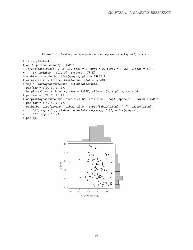
CHAPTER 4. R GRAPHICS REFERENCE
Figure 4.16: Creating multiple plots on one page using the layout() function.
> library(Hmisc)
> op <- par(no.readonly = TRUE)
> layout(matrix(c(1, 0, 3, 2), ncol = 2, nrow = 2, byrow = TRUE), widths = c(3,
+ 1), heights = c(1, 3), respect = TRUE)
> agehist <- with(pbc, hist(ageyrs, plot = FALSE))
> albumhist <- with(pbc, hist(album, plot = FALSE))
> top <- max(agehist$counts, albumhist$counts)
> par(mar = c(0, 3, 1, 1))
> barplot(albumhist$counts, axes = FALSE, ylim = c(0, top), space = 0)
> par(mar = c(3, 0, 1, 1))
> barplot(agehist$counts, axes = FALSE, xlim = c(0, top), space = 0, horiz = TRUE)
> par(mar = c(4, 4, 1, 1))
> with(pbc, plot(ageyrs ~ album, xlab = paste(label(album), " (", units(album),
+ ")", sep = ""), ylab = paste(label(ageyrs), " (", units(ageyrs),
+ ")", sep = "")))
> par(op)
2.0 2.5 3.0 3.5 4.0
3040
5060
7080
Serum Albumin (mg/dL)
Age
(ye
ars)
93
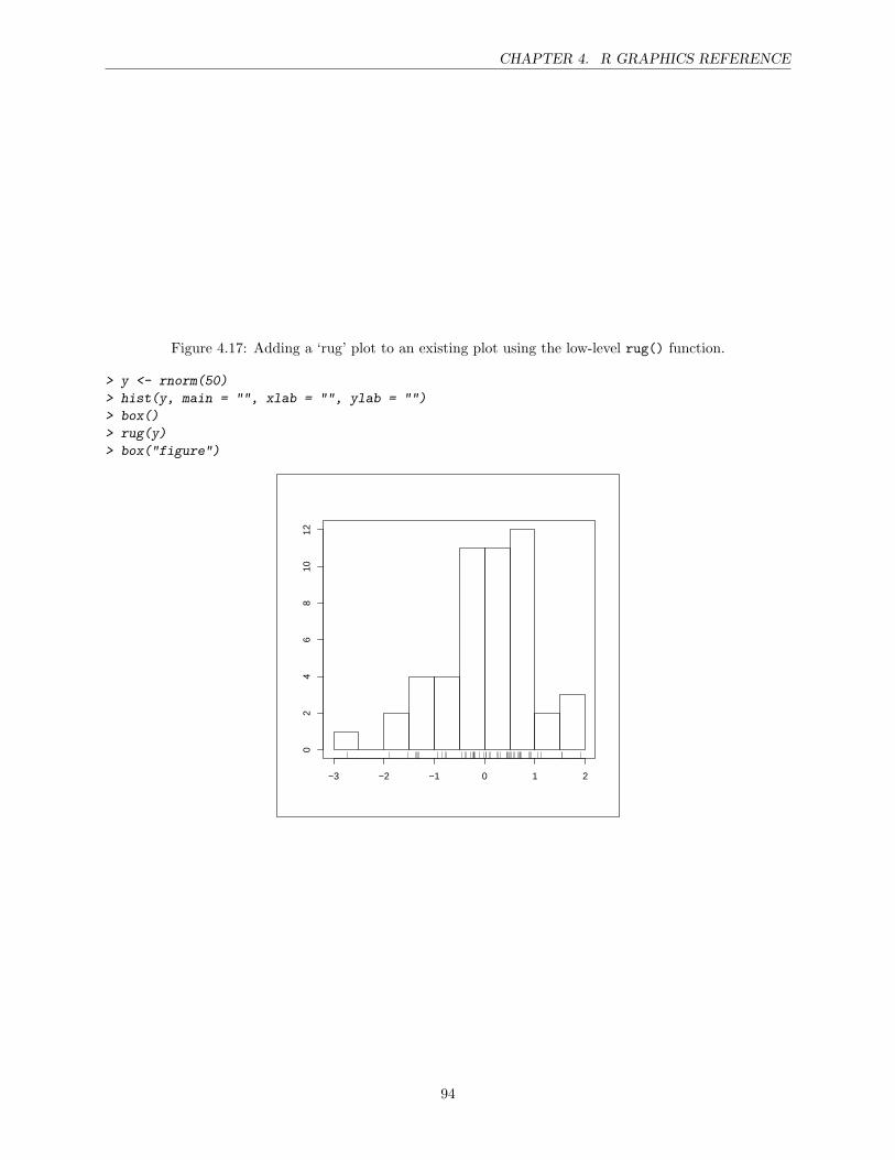
CHAPTER 4. R GRAPHICS REFERENCE
Figure 4.17: Adding a ‘rug’ plot to an existing plot using the low-level rug() function.
> y <- rnorm(50)
> hist(y, main = "", xlab = "", ylab = "")
> box()
> rug(y)
> box("figure")
−3 −2 −1 0 1 2
02
46
810
12
94

CHAPTER 4. R GRAPHICS REFERENCE
equal sign. We can also incorporate the paste() function into our expression – see Figure 4.19. Often, wewill want to replace some variable in a mathematical annotation with its values. To do this, we need to usethe substitute() function instead of the expression() function. We must specify the substitution using alist as a second argument and the value to be substituted must have previously been computed and assigneda name. See Figure 4.20 for an example.
GRAPHICAL OUTPUT: As demonstrated in the first document, when using R interactively, the mainpersistent record of graphical output is a window on your screen, which is also known as a GUI (‘graphicaluser interface’) screen device. When R is installed, an appropriate screen format is selected as the defaultscreen device and this default device is opened automatically the first time any graphical output occurs. Forexample, on the various Unix systems, the default GUI screen device is an X11 window. These GUI screendevices are opened by internally calling the x11(), windows(), and quartz() functions in the Linux/Unix,Windows, and Mac versions of R, respectively. By default, the size of an X11 graphics window and a Win-dows graphics window are 7 inches by 7 inches. A Mac graphics window is, by default, 5 inches by 5 inches.The three mentioned functions all have height= and width= arguments that can be used to open new screendevices of the desired size.
It is possible to have more than one screen device open at the same time, but only one device is currently‘active’ and all graphics output is sent to that device. If multiple devices are open, there are functions tocontrol which device is active. The screen devices are associated with a name (e.g., "X11" or "postscript")and a number – the "null device" is always device 1. The list of open devices can be obtained usingthe dev.list() function, which returns the name and number of all open devices, except device 1, the nulldevice. The dev.cur() function returns the number and name of only the active device, or 1, the null device,if none is active. The dev.set() function can be used to make a device active by specifying the appropriatedevice number. And the dev.next() and dev.prev() functions can be used to make the next/previousdevice on the device list the active device. Be aware, the display list can consume a reasonable amountof memory if a plot is particularly complex or if there are very many devices open at the same time. Thedev.off() shuts down the specified (by default the current) device, and the graphics.off() functions shutsdown all open graphics devices.
It is also possible to partition the active screen device with the split.screen() function. For exam-ple: split.screen(c(1, 2)) divides the device into two parts which can be selected with screen(1) orscreen(2). A part of the partitioned screen device can itself be divided again with the split.screen()function, which can make complex partitions. The erase.screen() function clears a single screen, andthe close.screen() removes the specified screen partition. These functions are totally incompatible withthe other mechanisms for arranging plots on a device (i.e., the par() function’s mfrow= argument and thelayout() function), and some plotting functions like the coplot() function.
Also, in the Windows version of R, you can save a ‘history’ of your graphs by activating the Recording featureunder the History drop-menu (seen when the graphics window is selected). You can then access old graphsby using the Page Up and Page Down keys.
As we mentioned in the first document, it is possible to produce a file that contains your plot. Similar tothe screen devices, the graphical output can be directed to a particular file device, which dictates the outputformat that will be produced. And like the screen devices, the file devices are controlled by specific functions:the postscript() function produces an Adobe PostScript file; the pdf() function produces an Adobe PDFfile; the pictex() function produces a LATEX PicTEX file; the xfig() function produces an XFIG file; thebitmap() function produces a GhostScript conversion to a file; the png() function produces a PNG bitmapfile; and the jpeg() function produces a JPEG bitmap file. On the Windows version of R, there are also thewin.metafile() and bmp() file device functions, which produce a Windows Metafile file and Windows BMPfile, respectively. Like the screen device functions, these file device functions allow you to specify things suchas the name of the file and the size of the plot.
95

CHAPTER 4. R GRAPHICS REFERENCE
Figure 4.18: Examples of mathematical annotation in a graph using the expression() function.
> par(mar = c(1, 1, 1, 1))
> plot(0:10, 0:10, type = "n", axes = FALSE)
> text(1, 10, expression(x %+-% y), cex = 1.5)
> text(1, 9, expression(x[i]), cex = 1.5)
> text(1, 8, expression(x^2), cex = 1.5)
> text(1, 7, expression(sqrt(x)), cex = 1.5)
> text(1, 6, expression(sqrt(x, 3)), cex = 1.5)
> text(1, 5, expression(x != y), cex = 1.5)
> text(1, 4, expression(x <= y), cex = 1.5)
> text(1, 3, expression(hat(x)), cex = 1.5)
> text(1, 2, expression(tilde(x)), cex = 1.5)
> text(1, 1, expression(bar(x)), cex = 1.5)
> text(1, 0, expression(x %<=>% y), cex = 1.5)
> text(4, 10, expression(Alpha + Omega), cex = 1.5)
> text(4, 9, expression(alpha + omega), cex = 1.5)
> text(4, 8, expression(45 * degree), cex = 1.5)
> text(4, 7, expression(frac(x, y)), cex = 1.5)
> text(4, 5.5, expression(sum(x[i], i = 1, n)), cex = 1.5)
> text(4, 4, expression(prod(plain(P)(X == x), x)), cex = 1.5)
> text(4, 2.5, expression(integral(f(x) * dx, a, b)), cex = 1.5)
> text(4, 0.5, expression(lim(f(x), x %->% 0)), cex = 1.5)
> text(8, 10, expression(x^y + z), cex = 1.5)
> text(8, 9, expression(x^(y + z)), cex = 1.5)
> text(8, 8, expression(x^
+ y + z
+ ), cex = 1.5)
> text(8, 6, expression(hat(beta) == (X^t * X)^
+ -1
+ * X^t * y), cex = 1.5)
> text(8, 4, expression(bar(x) == sum(frac(x[i], n), i == 1, n)), cex = 1.5)
> text(8, 2, expression(paste(frac(1, sigma * sqrt(2 * pi)), " ", plain(e)^
+ frac(-(x - mu)^2, 2 * sigma^2)
+ )), cex = 1.5)
> box("figure")
x ±± y
xi
x2
x
3 x
x ≠≠ y
x ≤≤ y
x
x~
x
x ⇔⇔ y
ΑΑ ++ ΩΩ
αα ++ ωω
45°°xy
∑∑1
nxi
∏∏x
P((X == x))
⌠⌠⌡⌡a
bf((x))dx
limx→→0
f((x))
xy ++ z
x((y++z))
xy++z
ββ == ((XtX))−−1Xty
x == ∑∑i==1
n xi
n
1
σσ 2ππ e
−−((x−−µµ))22σσ2
96

CHAPTER 4. R GRAPHICS REFERENCE
Figure 4.19: Examples of mathematical annotation in a graph using the paste() function in conjunctionwith the expression() function.
> x <- seq(-4, 4, length = 101)
> plot(x, sin(x), type = "l", xaxt = "n", xlab = expression(paste("Phase Angle ",
+ phi)), ylab = expression("sin " * phi))
> axis(side = 1, at = c(-pi, -pi/2, 0, pi/2, pi), label = expression(-pi,
+ -pi/2, 0, pi/2, pi))
> box("figure")
−1.
0−
0.5
0.0
0.5
1.0
Phase Angle φφ
sin
φφ
−− ππ −− ππ 2 0 ππ 2 ππ
97
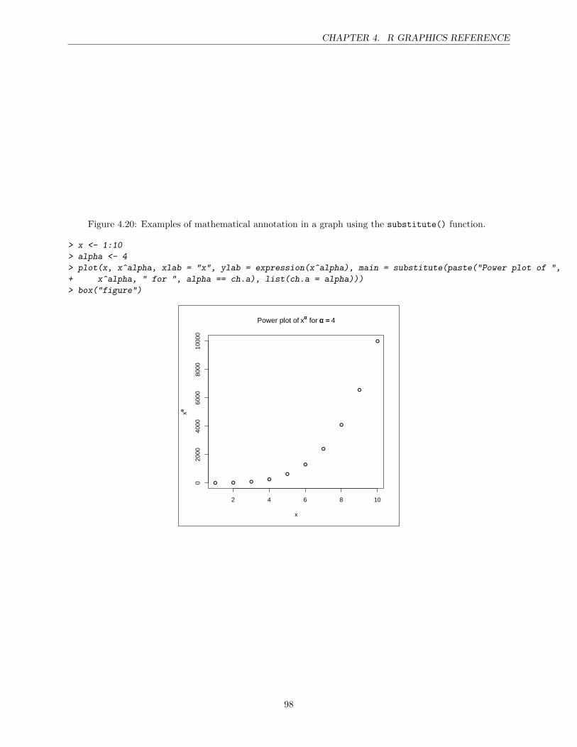
CHAPTER 4. R GRAPHICS REFERENCE
Figure 4.20: Examples of mathematical annotation in a graph using the substitute() function.
> x <- 1:10
> alpha <- 4
> plot(x, x^alpha, xlab = "x", ylab = expression(x^alpha), main = substitute(paste("Power plot of ",
+ x^alpha, " for ", alpha == ch.a), list(ch.a = alpha)))
> box("figure")
2 4 6 8 10
020
0040
0060
0080
0010
000
Power plot of xαα for αα == 4
x
xαα
98
CHAPTER 4. R GRAPHICS REFERENCE
Unlike sending graphical output to a window on your screen, directing graphical output to a file takes afew more steps. A file device must be created or ‘opened to writing’ in order to receive graphical outputby invoking the desired file device function with at least the desired file name specified. Once you haveopened the file to writing, you then compile all of your desired graphical function invocations. In turn,the specific file device that you opened converts the graphical function invocations from R (e.g., ‘draw aline’) into commands that the particular device can understand (e.g., PostScript commands if you used thepostscript() function). When you have finished writing the desired graphical output to a file, you thenclose the file to writing (and therefore close the file device) by invoking the dev.off() function. For example,let’s write a simple scatterplot to a PDF file named myplot.pdf:
> pdf("myplot.pdf", height = 8.5, width = 11)> with(pbc, plot(age.years ~ chol, main = "Age (years) vs. Serum Chol",+ xlab = label(chol), ylab = label(age.years)))> dev.off()
In the previous code, we also specified that the plot should be in a landscape orientation (i.e., height <width), with a height of 8.5” and a width of 11.0”.
Because all graphical output is directed to a file when using a file device function, it is best to use theappropriate screen device function to specify the size of the graphics window on your screen, and to directall intermediate iterations of the graphical output to the window. Once the graph has been ‘finalized,’ youcan then use one of the file device functions to write the graph to a file.
Also, when using the Windows version of R, you do not necessarily need to save the graph as its own fileusing a file device function. Specifically, in the Windows version of R, right-clicking on the graphics windowoffers you three options for outputting any desired graph from R: (1) Copy your graph as either a metafileor a bitmap; (2) Save your graph as either a metafile or postscript; and/or (3) Print your graph. For theCopy and Save options, it is very easy to then Paste or Insert, respectively, your graph into a Microsoft Wordand/or Powerpoint document.
For a screen device, starting a new page involves clearing the window before producing more output. On theother hand, only certain file devices allow multiple pages of output. For example, PostScript and PDF allowmultiple pages, but PNG does not. It is usually possible, especially for devices that do not support multiplepages of output, to specify that each page of output produces a separate file. This is achieved by specifyingthe argument onefile = FALSE when opening a device and specifying a pattern for the file name like file= "myplot%03d". The %03d is replaced by a three-digit number (padded with zeros) indicating the ‘pagenumber’ for each file that is created.
99