Embed Size (px)
Citation preview
An Introduction to theFundamentals & Functionality of
the R Programming Language
— Part I: An Overview —
Theresa A Scott, MSBiostatistician IIIDepartment of BiostatisticsVanderbilt University
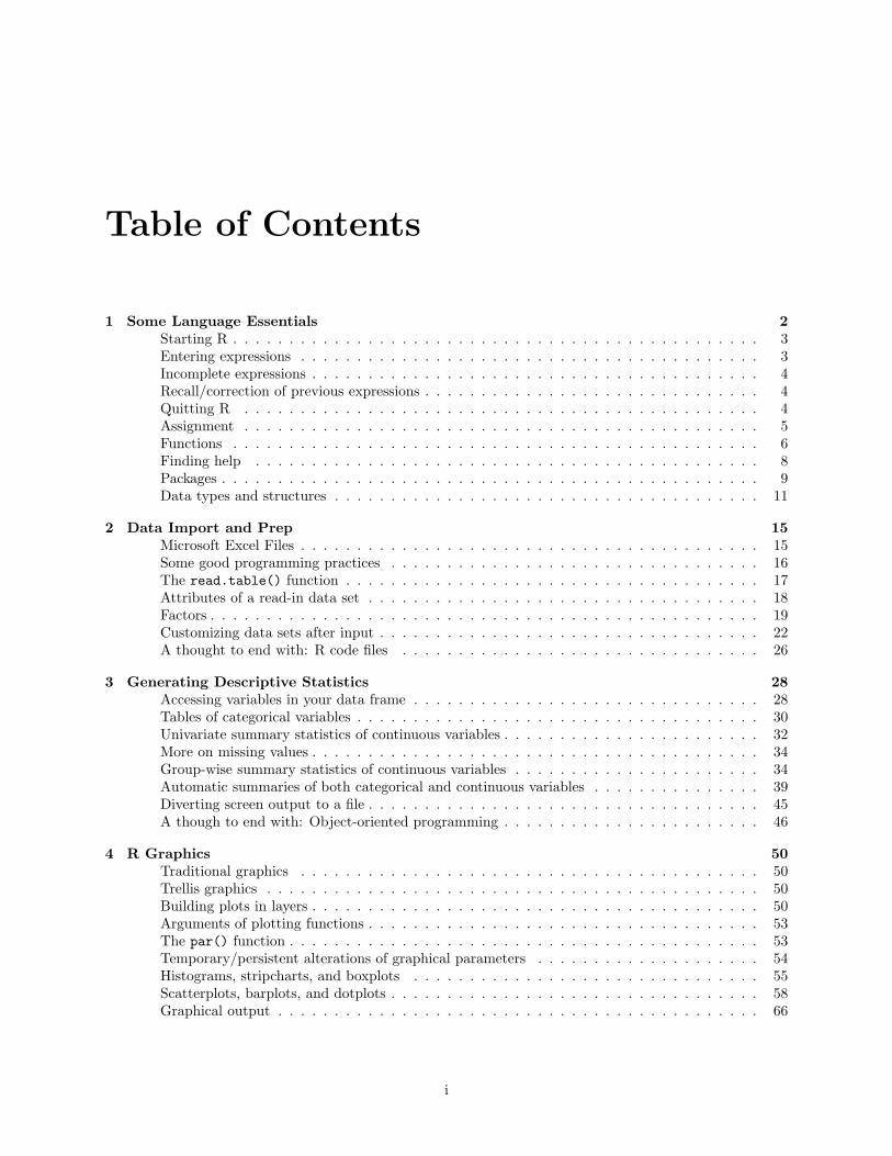
Table of Contents
1 Some Language Essentials 2Starting R . . . . . . . . . . . . . . . . . . . . . . . . . . . . . . . . . . . . . . . . . . . . . . . 3Entering expressions . . . . . . . . . . . . . . . . . . . . . . . . . . . . . . . . . . . . . . . . . 3Incomplete expressions . . . . . . . . . . . . . . . . . . . . . . . . . . . . . . . . . . . . . . . . 4Recall/correction of previous expressions . . . . . . . . . . . . . . . . . . . . . . . . . . . . . . 4Quitting R . . . . . . . . . . . . . . . . . . . . . . . . . . . . . . . . . . . . . . . . . . . . . . 4Assignment . . . . . . . . . . . . . . . . . . . . . . . . . . . . . . . . . . . . . . . . . . . . . . 5Functions . . . . . . . . . . . . . . . . . . . . . . . . . . . . . . . . . . . . . . . . . . . . . . . 6Finding help . . . . . . . . . . . . . . . . . . . . . . . . . . . . . . . . . . . . . . . . . . . . . 8Packages . . . . . . . . . . . . . . . . . . . . . . . . . . . . . . . . . . . . . . . . . . . . . . . . 9Data types and structures . . . . . . . . . . . . . . . . . . . . . . . . . . . . . . . . . . . . . . 11
2 Data Import and Prep 15Microsoft Excel Files . . . . . . . . . . . . . . . . . . . . . . . . . . . . . . . . . . . . . . . . . 15Some good programming practices . . . . . . . . . . . . . . . . . . . . . . . . . . . . . . . . . 16The read.table() function . . . . . . . . . . . . . . . . . . . . . . . . . . . . . . . . . . . . . 17Attributes of a read-in data set . . . . . . . . . . . . . . . . . . . . . . . . . . . . . . . . . . . 18Factors . . . . . . . . . . . . . . . . . . . . . . . . . . . . . . . . . . . . . . . . . . . . . . . . . 19Customizing data sets after input . . . . . . . . . . . . . . . . . . . . . . . . . . . . . . . . . . 22A thought to end with: R code files . . . . . . . . . . . . . . . . . . . . . . . . . . . . . . . . 26
3 Generating Descriptive Statistics 28Accessing variables in your data frame . . . . . . . . . . . . . . . . . . . . . . . . . . . . . . . 28Tables of categorical variables . . . . . . . . . . . . . . . . . . . . . . . . . . . . . . . . . . . . 30Univariate summary statistics of continuous variables . . . . . . . . . . . . . . . . . . . . . . . 32More on missing values . . . . . . . . . . . . . . . . . . . . . . . . . . . . . . . . . . . . . . . . 34Group-wise summary statistics of continuous variables . . . . . . . . . . . . . . . . . . . . . . 34Automatic summaries of both categorical and continuous variables . . . . . . . . . . . . . . . 39Diverting screen output to a file . . . . . . . . . . . . . . . . . . . . . . . . . . . . . . . . . . . 45A though to end with: Object-oriented programming . . . . . . . . . . . . . . . . . . . . . . . 46
4 R Graphics 50Traditional graphics . . . . . . . . . . . . . . . . . . . . . . . . . . . . . . . . . . . . . . . . . 50Trellis graphics . . . . . . . . . . . . . . . . . . . . . . . . . . . . . . . . . . . . . . . . . . . . 50Building plots in layers . . . . . . . . . . . . . . . . . . . . . . . . . . . . . . . . . . . . . . . . 50Arguments of plotting functions . . . . . . . . . . . . . . . . . . . . . . . . . . . . . . . . . . . 53The par() function . . . . . . . . . . . . . . . . . . . . . . . . . . . . . . . . . . . . . . . . . . 53Temporary/persistent alterations of graphical parameters . . . . . . . . . . . . . . . . . . . . 54Histograms, stripcharts, and boxplots . . . . . . . . . . . . . . . . . . . . . . . . . . . . . . . 55Scatterplots, barplots, and dotplots . . . . . . . . . . . . . . . . . . . . . . . . . . . . . . . . . 58Graphical output . . . . . . . . . . . . . . . . . . . . . . . . . . . . . . . . . . . . . . . . . . . 66
i
Preface
I have been using R since the summer of 2000 and have been trying to teach it to others for almost as long.When I was learning R (on my own) I got very frustrated with most of the existing R documentation. Inparticular, a lot of the documentation was written as a companion manuscript to an introductory statisticscourse. These and others covered the ‘fundamentals of R’ in a chapter or two and then spent the rest of theirtime demonstrating how to perform various statistical analyses using R. I felt they introduced you to someof the fundamentals, but very few discussed them extensively. I have also found over the years that, even asa full-time Biostatistician, 99% of my time is spent dealing with these fundamentals, not statistical analyses.Therefore, the purpose of this document and its companion is to introduce you to the fundamentals andfunctionality of the R programming language. The only statistics that will be covered is how to generatedescriptive statistics and some statistics related graphics.
This document and its companion are by no means an ‘original’ piece of work. I have merely assembledmuch of the existing documentation into my own set of documents. However, I have tried to present thetopics in a slightly different order than what is usually done. Specifically, the first document (‘An Overview’)covers some of the fundamentals, but then gets you right into the functionality – we read in a data set, makemodifications to it, summarize it with descriptive statistics, and generate various graphical depictions of it.The goal is that you will be very comfortable interacting with R by the end of the first document. The seconddocument (‘The Nuts & Bolts’) returns to the fundamentals, covering various topics in more depth. Thesecond document also includes a catalog of various R functions and an R graphics reference. Throughoutboth documents, I have also tried to include as much of my practical experience with R that I could.
I hope you find my group of documents helpful and hope they allow you to start using R confidently. YOucan find this document, it’s companion and other supporting files at http://biostat.mc.vanderbilt.edu/TheresaScott under Current Teaching Material. Feel free to contact me at [email protected] any questions and/or comments. I also welcome any suggestions and (constructive) criticism.
Lastly, the following is a crude list of the references I have used to compile this document and its companion:
� Contributed documents, manuals, frequently asked questions, and newsletters available via the Other,Manuals, FAQs, and Newsletter links under the Documentation header at the R website.
� Several books including1
– ‘An Introduction to R’ by WN Venables, et al.
– ‘Introductory Statistics with R’ by Peter Dalgaard.
– ‘R Graphics’ by Paul Murrell.
– ‘Using R for Introductory Statistics’ by John Verzani.
– ‘Statistics: An Introduction Using R by Michael J Crawley.
– ‘A Handbook of Statistical Analyses using R’ by Brian Everitt and Torsten Hothorn.
– ‘An R and S-Plus Companion to Applied Regression’ by John Fox.
– ‘Data Analysis and Graphics Using R’ by John Maindonald and John Braun.
1Note, a comprehensive list is available via the Books link under the same Documentation header at the R website.
1
Chapter 1
Some Language Essentials
Learning objectiveTo understand how to use R interactively and the language essentials of assignment, functions, and datastructures.
The goal of this document is to briefly introduce you to the very powerful facilities that the R programminglanguage provides. We cannot do this, however, without briefly covering some of the essentials of the Rlanguage.
R is a free interactive programming language and environment, created as an integrated suite of softwarefacilities for data manipulation, simulation, calculation, and graphical display. Even though R is mainly usedas a statistical analysis package, R is in no way limited to just statistics. As a side, R is an independent,open-source implementation of the S language. The commercial product S-PLUS is also based on S, and Rand S-PLUS are essentially identical.
The benefits of using R include:
� Its availability as free software – ‘free’ in terms of price, and (more importantly) in terms of freedomto run, copy, distribute, study, change, and improve the software.
� Its ability to run on Windows, MacOS, and Linux and UNIX platforms.
� The ability to completely reproduce your analysis and results, if properly documented, since the lan-guage is code driven. This is not always true with menu driven analysis packages; they are often muchharder to document.
� Its extendability – hundreds of libraries of functions to use, as well as the ability to write your ownfunctions.
� Its flexibility – unlike some classical software programs (e.g., SAS and SPSS), which display all theresults of an analysis, R allows you to assign any results to a (symbolic) variable, so that an analysiscan be done with minimal or no output, and the parts of the results of interest can be extracted andused in subsequent analyses.
� Its excellent graphing capabilities, including the ease with which well-designed publication-quality plotscan be produced.
For this course, you should have already installed R onto your laptop/computer – these notes were compiledusing R version 2.8.1 (2008-12-22). In general, both the complete instructions and the necessary accompa-nying files needed to install R are distributed by the Comprehensive R Archive Network (CRAN) on theirwebsite http://www.cran.r-project.org. See any of the following Documentation for detailed instruc-tions: the ‘R Installation and Administration’ document under the Manuals link; the FAQ link (both general
2
CHAPTER 1. SOME LANGUAGE ESSENTIALS
and Windows and Mac specific); and/or the ‘Installing R under Windows’ article in the June 2001 edition(Vol. 1/2; pages 11-14) Newsletter. NOTE: You will also need to have administrative rights to your lap-top/computer in order to successfully install a package, which we will cover via a practice exercise.
Before going further, it is helpful to interact with R on the simplest level – that is, using it as a calculator.The following session is intended to introduce you to some of the features of the R environment by using them.
STARTING R: When using the Windows or Mac versions of R, launch R by double-clicking the R iconon the desktop, or by finding the R program under the start menu. This will start R in a new consolewindow with a command line subwindow. On the other hand, when using the Linux/Unix version of R,launch R by typing ‘R’ at the shell command prompt (i.e., ‘$ R’ if we assume that the shell prompt is ‘$’)of a terminal window. This will cause R to start up as an interactive program in the current terminal window.
→ Practice Exercise: Go ahead and start R using one of the mentioned methods that is appropriate for yourtype of laptop/computer.
ENTERING EXPRESSIONS: There are several ways to interact with R, but the simplest way is totype expressions at the cursor following the command line prompt, which is denoted by the greater thansymbol, >. To evaluate the expression, we simply press the ENTER key. The simplest expressions to enterat the command line are arithmetic expressions involving numbers and algebraic operators. R includes theusual arithmetic operators: + (addition), - (subtraction), * (multiplication), / (division), and ^ (exponen-tiation). Note, unlike most arithmetic operators, the exponentiation operator, ^, works from the right tothe left – 2^2^3 = 28 not 43. The set of arithmetic operators also includes %% (modulo) and %/% (integerdivision). In addition, (1) instead of using a newline, (short) expressions can be separated by a semi-colon(;); and (2) parentheses can be used to group expressions, altering the order in which expression are evaluated.
→ Practice Exercise: Type any of the following arithmetic expression at the command line and press ENTERor try any of your own.
> 2 * 10
[1] 20
> 10 + 13 - 21
[1] 2
> 2^3
[1] 8
> 1 - 2 * 3
[1] -5
> (1 - 2) * 3
[1] -3
As we see, the output of each evaluated expression is printed (and lost). In addition, the printed outputmay appear odd. The [1] in front of the output is part of R’s way of printing intrinsic data structures tothe screen. More specifically, when printed output consists of many values spread over several lines, eachline begins with the index (number) of the first element of the line. You also probably noticed the additionalspaces around some of the arithmetic operators. Although spaces are not required to separate elements ofan arithmetic expression (i.e., are ignored), judicious use of spaces can help to clarify the meaning of theexpression.
3
CHAPTER 1. SOME LANGUAGE ESSENTIALS
EXPRESSION EVALUATION: R evaluates expressions using a type of question-and-answer model.Specifically, when you type an expression at the command line prompt and press ENTER, the commandis first transformed by R into an internal representation. If the expression is syntactically complete, thetransformed expression is then executed and R returns (prints) the result value of the expression to thescreen. Once executed, R then asks for more input by printing the command line prompt and cursor. Infuture sections, we will see that not all expressions return (print) a result value.
INCOMPLETE EXPRESSIONS: If an expression is not syntactically complete when ENTER is pressed,R will print the continuation prompt, +, at the beginning of the second and subsequent lines and continueto read input until the expression is syntactically complete.
→ Practice Exercise: To demonstrate how R reacts to incomplete expressions, type in the mathematicalexpression 2 + 3 + 5 - 2 at the command line by hitting the ENTER key after each arithmetic operator:
> 2 ++ 3 ++ 5 -+ 2[1] 8
The other main reasons why an expression may be incomplete are because of unmatched parentheses and/orquotation marks. In the Windows/Mac versions of R, use the Esc key to cancel an incomplete expression,which will print a new command line prompt and cursor. In the Unix/Linux version of R, use Ctrl-C.
RECALL/CORRECTION OF PREVIOUS EXPRESSIONS: Using the command line in R can in-volve a fair amount of typing. However, there are ways to reduce the amount of necessary typing. Specifically,the R console keeps a history of the expressions entered, which is known as the command history. Individu-ally, the expressions can be accessed using the up- and down-arrow keys. Repeatedly pushing the up-arrowwill scroll backwards through the command history. With the up- and down-arrow keys we can access thedesired previous expression and then edit it as desired using keys like the left- and right-arrow keys, theHome and End keys (or Ctrl-a and Ctrl-e, respectively), and the Backspace and Delete keys. Another usefulkeyboard shortcut to use in conjunction with the Home key/Ctrl-a is Ctrl-k, which ‘kills’ (deletes) the currentline (if the cursor is at the beginning of the line).
→ Practice Exercise: Using the up-arrow key, recall one of your previous arithmetic expressions, and usethe left- and right-arrow keys, the Home and End keys, and the Backspace and Delete keys to modify andre-evaluate the expression.
QUITTING R: Lastly, to quit R, type q() at the command line prompt – you must include the paren-theses (‘()’). You will then be asked Save workspace image?. Answer “No” by clicking the No button ortyping n. Don’t worry if this doesn’t make a lot of sense right now; we’ll be discuss it more in the ‘ObjectManagement’ section of the second document. NOTE: When we type q() and hit ENTER, we are actuallyexecuting the quit function. We will be discussing functions in more detail soon.
THE GRAMMAR OF EXPRESSIONS: Up to this point, all of the expressions we have entered at thecommand line have been simple mathematical expressions involving only numbers and arithmetic operators.Also, up to this point, the result of each evaluated expression has been printed and then discarded. Obvi-ously, we need to be able to use R as more than just a calculator. Specifically, we need to be able to (amongother things): (1) retain the results of specific evaluated expressions; (2) use data that consists of morethan one number; and (3) possess the tools to carry out a variety of desired tasks. The solution to these de-sires will involve evaluating expressions that include (1) assignment, (2) functions, and/or (3) data structures.
TERMINOLOGY – ‘object’: We will use the term object quite often in future sections. You can thinkof an object as anything in R that is returned (printed) by an evaluated expression, anything that you define
4
CHAPTER 1. SOME LANGUAGE ESSENTIALS
via assignment, or anything that is already defined by R (i.e., functions).
ASSIGNMENT: R allows values to be assigned a (symbolic) name, which allows the name to be used torepresent that value in subsequent expressions. The simplest example would be to assign the value of 5 tothe name ‘x’ using the assignment operator (<-):
> x <- 5
The expression x <- 5 can be read as “the name x is assigned the value 5.” The assignment operator <-consists of a less than sign (<) followed by a minus sign (-) without any spaces between them. The less thansign ‘points’ to the name receiving the value. In general, no result is printed when a name is assigned to avalue. In order to print the value of the evaluated expression, we must enter the name of the value at thecommand line.
> x
[1] 5
A way to evaluate the assignment and to print the evaluated result is to wrap the assignment expressionwith a set of parentheses. For example,
> (x <- 5)
[1] 5
As mentioned, once a value has been assigned to a name, that name can be used to represent the value insubsequent expressions:
> 10 * x + 2
[1] 52
A name can also be ‘re-assigned ’ at any time, and the old value is overwritten with the new:
> x
[1] 5
> x <- 2
> x
[1] 2
As we saw with our arithmetic expressions, spacing around operators is generally disregarded by R, butnotice that adding a space in the middle of an assignment operator <- changes the meaning to ‘less than’followed by ‘minus’ (conversely, omitting the space when comparing a variable to a negative number hasunexpected consequences). As an example,
> x < -5
[1] FALSE
→ Practice Exercise: At the command line, work through a similar example by assigning the value 10 tothe name ‘y’, evaluating the expression y^2 + 20, and re-assigning the name ‘y’ to the value 8.
IMPORTANT: The value we assign to a name is not limited to a single value. In general, the evalu-ated value of any expression, which is commonly referred to as an object, can be assigned to a name. Forexample, in future sections, we will assign a name to our read-in data set, which will allow us to refer toour data set by name in all subsequent expressions. Another example would be to assign a name to the
5
CHAPTER 1. SOME LANGUAGE ESSENTIALS
output of a regression model in order to use certain portions of the model output in subsequent expressions.In the same sense, an expression is allowed to be on the target side (left side) of an assignment, not just a(symbolic) name. For example, we can replace (re-assign) the missing values of a variable with a value of zero.
NAMING OBJECTS: There are some limitations as to what can be used to name an object. Specifically,object names (1) may consist of letters (A-Z and a-z), digits (0-9), periods (‘.’), and the underscore (‘_’);and (2) must not start with a digit nor underscore, nor with a period followed by a digit. Mathematicaloperators, such as +, -, ∗, and /, in addition to other special characters are also not allowed to be used inobject names. And DON’T FORGET , R is case sensitive – so, x and X are two distinct objects.
FUNCTIONS: Almost everything in R is done by invoking functions. Functions in R can do three things:(1) have values passed to them; (2) return a value; and/or (3) generate side effects, which are anything thatis not the returning of a value. Examples of functions that generate side effects are printing and plottingfunctions. Every function in R, whether intrinsic to the language or user-written, is defined using the samebasic statement: FUNname <- function( arglist ) { body }, where FUNname is the name of the function;arglist is a comma separated list of zero or more arguments that can be passed to the function; and body
contains the expressions that perform the actions of the function. In turn, the format to invoke a function isto type its name followed by a set of parentheses containing zero or more arguments. In other words, we canthink of calculus with its mathematical functions like f(x) or g(x, y). As John Verzani put it in his book,‘functions are like pets’ – they don’t come (aren’t invoked) unless we call them by name (case-sensitive andspelled properly); they have a mouth (the parentheses) that likes to be fed (the arguments to the function),and they will complain if they are not fed properly (the output of warnings and/or errors). BE AWARE:
1. Because R is case sensitive, so are the names of functions. So, for example, the reshape() andreShape() functions are two distinct functions.
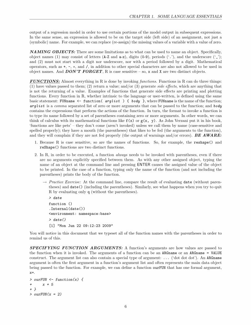
2. In R, in order to be executed, a function always needs to be invoked with parentheses, even if thereare no arguments explicitly specified between them. As with any other assigned object, typing thename of an object at the command line and pressing ENTER causes the assigned value of the objectto be printed. In the case of a function, typing only the name of the function (and not including theparentheses) prints the body of the function.
→ Practice Exercise: At the command line, compare the result of evaluating date (without paren-theses) and date() (including the parentheses). Similarly, see what happens when you try to quitR by evaluating only q (without the parentheses).> date
function ().Internal(date())<environment: namespace:base>
> date()
[1] "Mon Jun 22 09:12:23 2009"
You will notice in this document that we typeset all of the function names with the parentheses in order toremind us of this.
SPECIFYING FUNCTION ARGUMENTS: A function’s arguments are how values are passed tothe function when it is invoked. The arguments of a function can be an ARGname or an ARGname = VALUEconstruct. The argument list can also contain a special type of argument: ... (‘dot dot dot’). An ARGnameargument is often the first argument in a function’s argument list and often represents the main data objectbeing passed to the function. For example, we can define a function ourFUN that has one formal argument,x=.
> ourFUN <- function(x) {
+ x + 5
+ }
> ourFUN(x = 2)
6
CHAPTER 1. SOME LANGUAGE ESSENTIALS
[1] 7
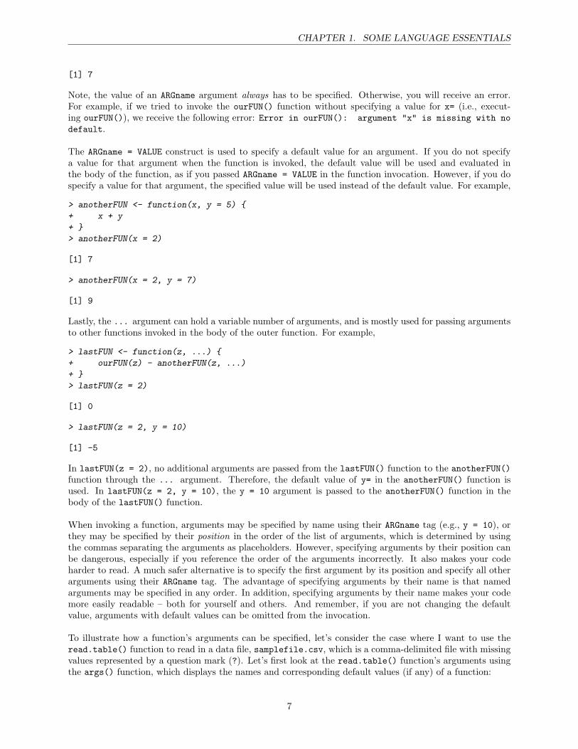
Note, the value of an ARGname argument always has to be specified. Otherwise, you will receive an error.For example, if we tried to invoke the ourFUN() function without specifying a value for x= (i.e., execut-ing ourFUN()), we receive the following error: Error in ourFUN(): argument "x" is missing with nodefault.
The ARGname = VALUE construct is used to specify a default value for an argument. If you do not specifya value for that argument when the function is invoked, the default value will be used and evaluated inthe body of the function, as if you passed ARGname = VALUE in the function invocation. However, if you dospecify a value for that argument, the specified value will be used instead of the default value. For example,
> anotherFUN <- function(x, y = 5) {
+ x + y
+ }
> anotherFUN(x = 2)
[1] 7
> anotherFUN(x = 2, y = 7)
[1] 9
Lastly, the ... argument can hold a variable number of arguments, and is mostly used for passing argumentsto other functions invoked in the body of the outer function. For example,
> lastFUN <- function(z, ...) {
+ ourFUN(z) - anotherFUN(z, ...)
+ }
> lastFUN(z = 2)
[1] 0
> lastFUN(z = 2, y = 10)
[1] -5
In lastFUN(z = 2), no additional arguments are passed from the lastFUN() function to the anotherFUN()function through the ... argument. Therefore, the default value of y= in the anotherFUN() function isused. In lastFUN(z = 2, y = 10), the y = 10 argument is passed to the anotherFUN() function in thebody of the lastFUN() function.
When invoking a function, arguments may be specified by name using their ARGname tag (e.g., y = 10), orthey may be specified by their position in the order of the list of arguments, which is determined by usingthe commas separating the arguments as placeholders. However, specifying arguments by their position canbe dangerous, especially if you reference the order of the arguments incorrectly. It also makes your codeharder to read. A much safer alternative is to specify the first argument by its position and specify all otherarguments using their ARGname tag. The advantage of specifying arguments by their name is that namedarguments may be specified in any order. In addition, specifying arguments by their name makes your codemore easily readable – both for yourself and others. And remember, if you are not changing the defaultvalue, arguments with default values can be omitted from the invocation.
To illustrate how a function’s arguments can be specified, let’s consider the case where I want to use theread.table() function to read in a data file, samplefile.csv, which is a comma-delimited file with missingvalues represented by a question mark (?). Let’s first look at the read.table() function’s arguments usingthe args() function, which displays the names and corresponding default values (if any) of a function:
7
CHAPTER 1. SOME LANGUAGE ESSENTIALS
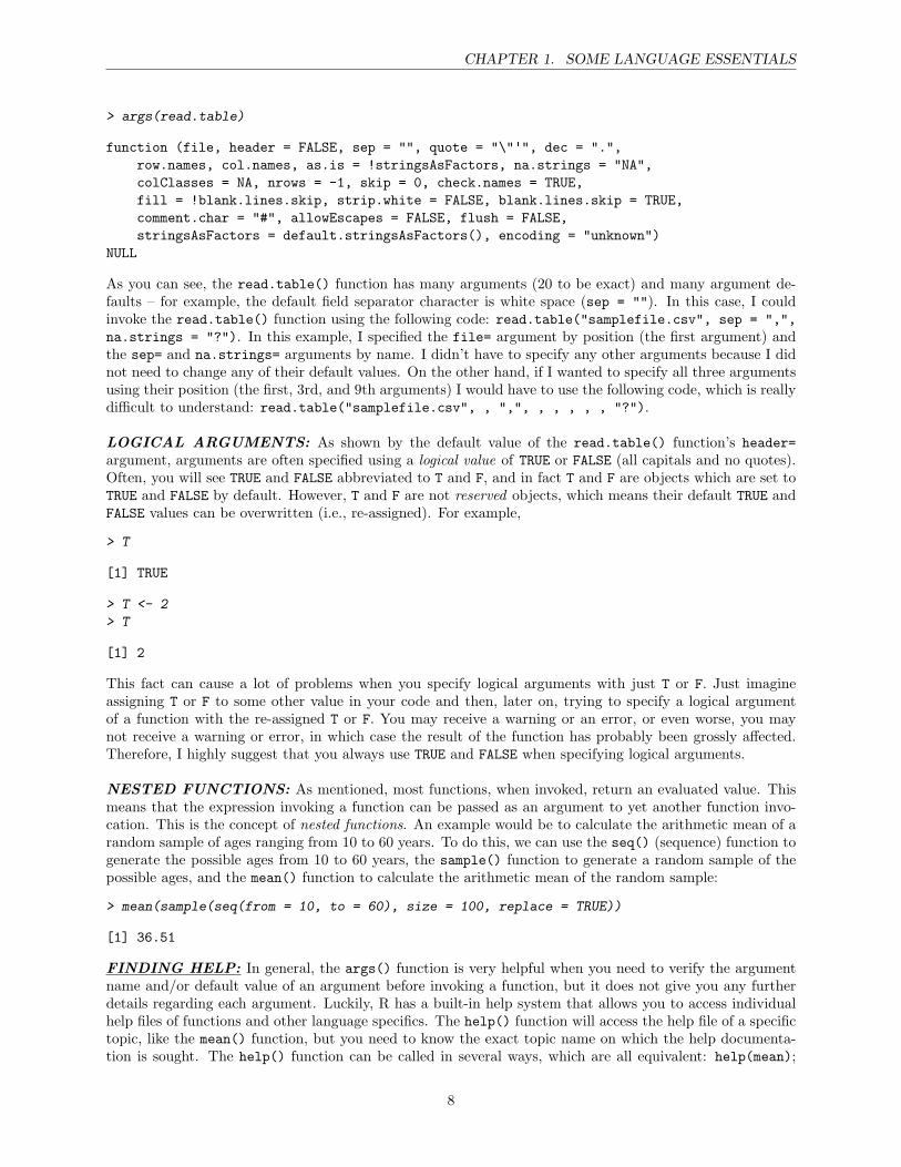
> args(read.table)
function (file, header = FALSE, sep = "", quote = "\"'", dec = ".",row.names, col.names, as.is = !stringsAsFactors, na.strings = "NA",colClasses = NA, nrows = -1, skip = 0, check.names = TRUE,fill = !blank.lines.skip, strip.white = FALSE, blank.lines.skip = TRUE,comment.char = "#", allowEscapes = FALSE, flush = FALSE,stringsAsFactors = default.stringsAsFactors(), encoding = "unknown")
NULL
As you can see, the read.table() function has many arguments (20 to be exact) and many argument de-faults – for example, the default field separator character is white space (sep = ""). In this case, I couldinvoke the read.table() function using the following code: read.table("samplefile.csv", sep = ",",na.strings = "?"). In this example, I specified the file= argument by position (the first argument) andthe sep= and na.strings= arguments by name. I didn’t have to specify any other arguments because I didnot need to change any of their default values. On the other hand, if I wanted to specify all three argumentsusing their position (the first, 3rd, and 9th arguments) I would have to use the following code, which is reallydifficult to understand: read.table("samplefile.csv", , ",", , , , , , "?").
LOGICAL ARGUMENTS: As shown by the default value of the read.table() function’s header=argument, arguments are often specified using a logical value of TRUE or FALSE (all capitals and no quotes).Often, you will see TRUE and FALSE abbreviated to T and F, and in fact T and F are objects which are set toTRUE and FALSE by default. However, T and F are not reserved objects, which means their default TRUE andFALSE values can be overwritten (i.e., re-assigned). For example,
> T
[1] TRUE
> T <- 2
> T
[1] 2
This fact can cause a lot of problems when you specify logical arguments with just T or F. Just imagineassigning T or F to some other value in your code and then, later on, trying to specify a logical argumentof a function with the re-assigned T or F. You may receive a warning or an error, or even worse, you maynot receive a warning or error, in which case the result of the function has probably been grossly affected.Therefore, I highly suggest that you always use TRUE and FALSE when specifying logical arguments.
NESTED FUNCTIONS: As mentioned, most functions, when invoked, return an evaluated value. Thismeans that the expression invoking a function can be passed as an argument to yet another function invo-cation. This is the concept of nested functions. An example would be to calculate the arithmetic mean of arandom sample of ages ranging from 10 to 60 years. To do this, we can use the seq() (sequence) function togenerate the possible ages from 10 to 60 years, the sample() function to generate a random sample of thepossible ages, and the mean() function to calculate the arithmetic mean of the random sample:
> mean(sample(seq(from = 10, to = 60), size = 100, replace = TRUE))
[1] 36.51
FINDING HELP: In general, the args() function is very helpful when you need to verify the argumentname and/or default value of an argument before invoking a function, but it does not give you any furtherdetails regarding each argument. Luckily, R has a built-in help system that allows you to access individualhelp files of functions and other language specifics. The help() function will access the help file of a specifictopic, like the mean() function, but you need to know the exact topic name on which the help documenta-tion is sought. The help() function can be called in several ways, which are all equivalent: help(mean);
8
CHAPTER 1. SOME LANGUAGE ESSENTIALS
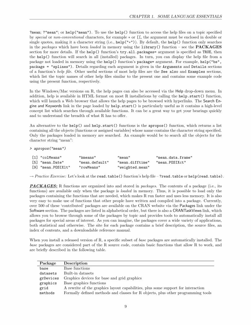
?mean; ?"mean"; or help("mean"). To use the help() function to access the help files on a topic specifiedby special or non-conventional characters, for example ∗ or [[, the argument must be enclosed in double orsingle quotes, making it a character string (i.e., help("∗")). By default, the help() function only searchesin the packages which have been loaded in memory using the library() function – see the PACKAGESsection for more details. If the help() function’s try.all.packages= argument is specified as TRUE, thenthe help() function will search in all (installed) packages. In turn, you can display the help file from apackage not loaded in memory using the help() function’s package= argument. For example, help("bs",package = "splines"). Details regarding each argument is given in the Arguments and Details sectionsof a function’s help file. Other useful sections of most help files are the See also and Examples sections,which list the topic names of other help files similar to the present one and contains some example codeusing the present function, respectively.
In the Windows/Mac versions on R, the help pages can also be accessed via the Help drop-down menu. Inaddition, help is available in HTML format on most R installations by calling the help.start() function,which will launch a Web browser that allows the help pages to be browsed with hyperlinks. The Search En-gine and Keywords link in the page loaded by help.start() is particularly useful as it contains a high-levelconcept list which searches through available functions. It can be a great way to get your bearings quicklyand to understand the breadth of what R has to offer.
An alternative to the help() and help.start() functions is the apropos() function, which returns a listcontaining all the objects (functions or assigned variables) whose name contains the character string specified.Only the packages loaded in memory are searched. An example would be to search all the objects for thecharacter string “mean”:
> apropos("mean")
[1] "colMeans" "kmeans" "mean" "mean.data.frame"[5] "mean.Date" "mean.default" "mean.difftime" "mean.POSIXct"[9] "mean.POSIXlt" "rowMeans" "weighted.mean"
→ Practice Exercise: Let’s look at the read.table() function’s help file – ?read.table or help(read.table).
PACKAGES: R functions are organized into and stored in packages. The contents of a package (i.e., itsfunctions) are available only when the package is loaded in memory. Thus, it is possible to load only thepackages containing the functions that are needed, which makes R run faster and uses less memory. It is alsovery easy to make use of functions that other people have written and compiled into a package. Currently,over 500 of these ‘contributed’ packages are available on the CRAN website via the Packages link under theSoftware section. The packages are listed in alphabetical order, but there is also a CRANTaskViews link, whichallows you to browse through some of the packages by topic and provides tools to automatically install allpackages for special areas of interest. As you can imagine, the packages cover a wide variety of applications,both statistical and otherwise. The site for each package contains a brief description, the source files, anindex of contents, and a downloadable reference manual.
When you install a released version of R, a specific subset of base packages are automatically installed. Thebase packages are considered part of the R source code, contain basic functions that allow R to work, andare briefly described in the following table.
Package Descriptionbase Base functionsdatasets Built-in datasetsgrDevices Graphics devices for base and grid graphicsgraphics Base graphics functionsgrid A rewrite of the graphics layout capabilities, plus some support for interactionmethods Formally defined methods and classes for R objects, plus other programming tools
9
CHAPTER 1. SOME LANGUAGE ESSENTIALS
splines Regression spline functions and classesstats Statistical functionsstats4 Statistical Functions using ‘S4 Classes’tools Tools for package development and administrationutils Utility functions
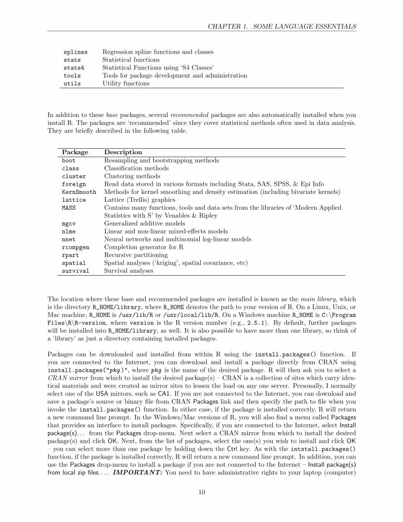
In addition to these base packages, several recommended packages are also automatically installed when youinstall R. The packages are ‘recommended’ since they cover statistical methods often used in data analysis.They are briefly described in the following table.
Package Descriptionboot Resampling and bootstrapping methodsclass Classification methodscluster Clustering methodsforeign Read data stored in various formats including Stata, SAS, SPSS, & Epi InfoKernSmooth Methods for kernel smoothing and density estimation (including bivariate kernels)lattice Lattice (Trellis) graphicsMASS Contains many functions, tools and data sets from the libraries of ‘Modern Applied
Statistics with S’ by Venables & Ripleymgcv Generalized additive modelsnlme Linear and non-linear mixed-effects modelsnnet Neural networks and multinomial log-linear modelsrcompgen Completion generator for Rrpart Recursive partitioningspatial Spatial analyses (‘kriging’, spatial covariance, etc)survival Survival analyses
The location where these base and recommended packages are installed is known as the main library, whichis the directory R_HOME/library, where R_HOME denotes the path to your version of R. On a Linux, Unix, orMac machine, R_HOME is /usr/lib/R or /usr/local/lib/R. On a Windows machine R_HOME is C:\ProgramFiles\R\R-version, where version is the R version number (e.g., 2.5.1). By default, further packageswill be installed into R_HOME/library, as well. It is also possible to have more than one library, so think ofa ‘library’ as just a directory containing installed packages.
Packages can be downloaded and installed from within R using the install.packages() function. Ifyou are connected to the Internet, you can download and install a package directly from CRAN usinginstall.packages("pkg )", where pkg is the name of the desired package. R will then ask you to select aCRAN mirror from which to install the desired package(s) – CRAN is a collection of sites which carry iden-tical materials and were created as mirror sites to lessen the load on any one server. Personally, I normallyselect one of the USA mirrors, such as CA1. If you are not connected to the Internet, you can download andsave a package’s source or binary file from CRAN Packages link and then specify the path to file when youinvoke the install.packages() function. In either case, if the package is installed correctly, R will returna new command line prompt. In the Windows/Mac versions of R, you will also find a menu called Packagesthat provides an interface to install packages. Specifically, if you are connected to the Internet, select Installpackage(s). . . from the Packages drop-menu. Next select a CRAN mirror from which to install the desiredpackage(s) and click OK. Next, from the list of packages, select the one(s) you wish to install and click OK– you can select more than one package by holding down the Ctrl key. As with the intstall.packages()function, if the package is installed correctly, R will return a new command line prompt. In addition, you canuse the Packages drop-menu to install a package if you are not connected to the Internet – Install package(s)from local zip files. . . . IMPORTANT: You need to have administrative rights to your laptop (computer)
10
CHAPTER 1. SOME LANGUAGE ESSENTIALS
in order to successfully install a package.
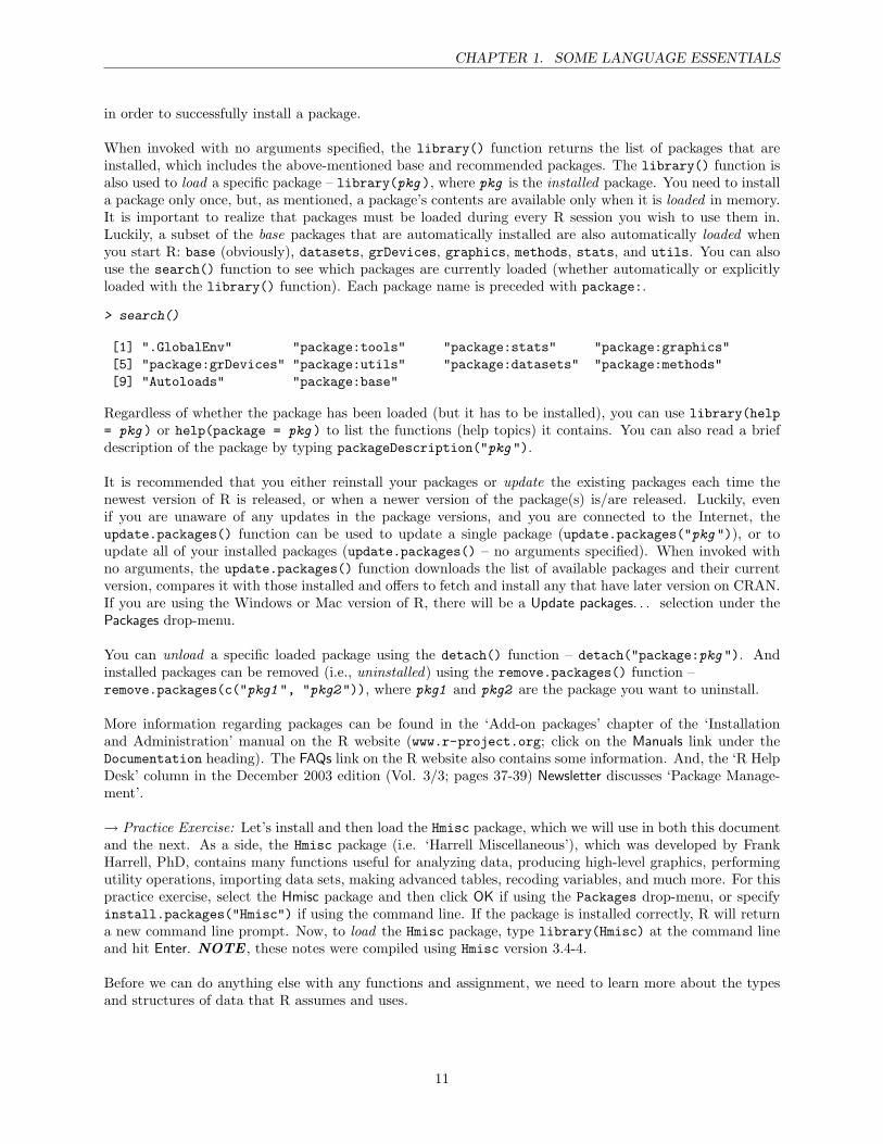
When invoked with no arguments specified, the library() function returns the list of packages that areinstalled, which includes the above-mentioned base and recommended packages. The library() function isalso used to load a specific package – library(pkg ), where pkg is the installed package. You need to installa package only once, but, as mentioned, a package’s contents are available only when it is loaded in memory.It is important to realize that packages must be loaded during every R session you wish to use them in.Luckily, a subset of the base packages that are automatically installed are also automatically loaded whenyou start R: base (obviously), datasets, grDevices, graphics, methods, stats, and utils. You can alsouse the search() function to see which packages are currently loaded (whether automatically or explicitlyloaded with the library() function). Each package name is preceded with package:.
> search()
[1] ".GlobalEnv" "package:tools" "package:stats" "package:graphics"[5] "package:grDevices" "package:utils" "package:datasets" "package:methods"[9] "Autoloads" "package:base"
Regardless of whether the package has been loaded (but it has to be installed), you can use library(help= pkg ) or help(package = pkg ) to list the functions (help topics) it contains. You can also read a briefdescription of the package by typing packageDescription("pkg ").
It is recommended that you either reinstall your packages or update the existing packages each time thenewest version of R is released, or when a newer version of the package(s) is/are released. Luckily, evenif you are unaware of any updates in the package versions, and you are connected to the Internet, theupdate.packages() function can be used to update a single package (update.packages("pkg ")), or toupdate all of your installed packages (update.packages() – no arguments specified). When invoked withno arguments, the update.packages() function downloads the list of available packages and their currentversion, compares it with those installed and offers to fetch and install any that have later version on CRAN.If you are using the Windows or Mac version of R, there will be a Update packages. . . selection under thePackages drop-menu.
You can unload a specific loaded package using the detach() function – detach("package:pkg "). Andinstalled packages can be removed (i.e., uninstalled) using the remove.packages() function –remove.packages(c("pkg1 ", "pkg2 ")), where pkg1 and pkg2 are the package you want to uninstall.
More information regarding packages can be found in the ‘Add-on packages’ chapter of the ‘Installationand Administration’ manual on the R website (www.r-project.org; click on the Manuals link under theDocumentation heading). The FAQs link on the R website also contains some information. And, the ‘R HelpDesk’ column in the December 2003 edition (Vol. 3/3; pages 37-39) Newsletter discusses ‘Package Manage-ment’.
→ Practice Exercise: Let’s install and then load the Hmisc package, which we will use in both this documentand the next. As a side, the Hmisc package (i.e. ‘Harrell Miscellaneous’), which was developed by FrankHarrell, PhD, contains many functions useful for analyzing data, producing high-level graphics, performingutility operations, importing data sets, making advanced tables, recoding variables, and much more. For thispractice exercise, select the Hmisc package and then click OK if using the Packages drop-menu, or specifyinstall.packages("Hmisc") if using the command line. If the package is installed correctly, R will returna new command line prompt. Now, to load the Hmisc package, type library(Hmisc) at the command lineand hit Enter. NOTE , these notes were compiled using Hmisc version 3.4-4.
Before we can do anything else with any functions and assignment, we need to learn more about the typesand structures of data that R assumes and uses.
11
CHAPTER 1. SOME LANGUAGE ESSENTIALS
DATA TYPES & STRUCTURES: As we have seen, R recognizes a number when we type one. Thisalso includes negative numbers (e.g., -2). To specify a piece of text (also called a character string), type itwithin either single or double quotes, such as ‘cat’ or "Drug X". R also recognizes logical values (also calledboolean values), which are typed as TRUE and FALSE (all capitals and no quotes). And there is a specialvalue, NA, which represents a missing or unknown value (again, no quotes). There are also three other specialconstants: (1) NULL, which is used to indicate an empty object; (2) Inf, which denotes infinity; and (3) NaN(‘not a number’), which is produced by numerical computations whose results is undefined (e.g., 1/0, 0/0,or Inf - Inf).
In addition to these basic types of data, R provides a number of data structures that allow multiple valuesto be specified as a single object. The data structures are vectors, matrices, arrays, data frames, and lists.In this document, we will work with vectors, data frames, and lists (briefly). We will discuss all of the datastructures in more detail in the next document.
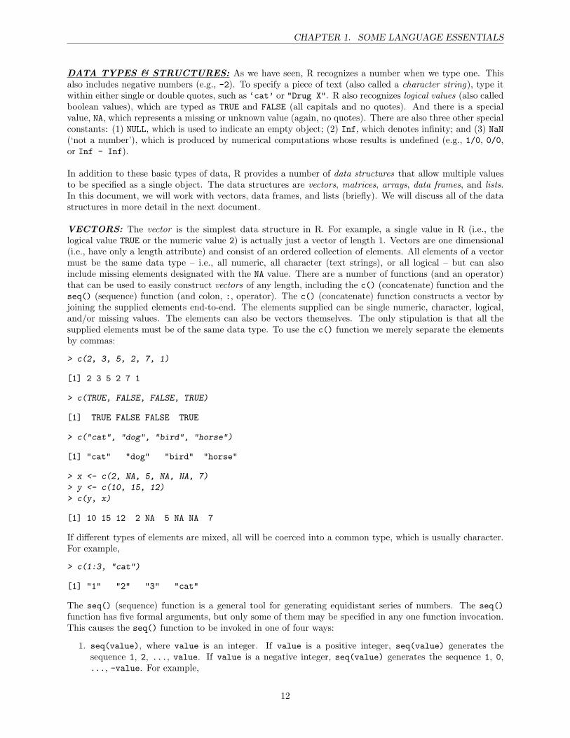
VECTORS: The vector is the simplest data structure in R. For example, a single value in R (i.e., thelogical value TRUE or the numeric value 2) is actually just a vector of length 1. Vectors are one dimensional(i.e., have only a length attribute) and consist of an ordered collection of elements. All elements of a vectormust be the same data type – i.e., all numeric, all character (text strings), or all logical – but can alsoinclude missing elements designated with the NA value. There are a number of functions (and an operator)that can be used to easily construct vectors of any length, including the c() (concatenate) function and theseq() (sequence) function (and colon, :, operator). The c() (concatenate) function constructs a vector byjoining the supplied elements end-to-end. The elements supplied can be single numeric, character, logical,and/or missing values. The elements can also be vectors themselves. The only stipulation is that all thesupplied elements must be of the same data type. To use the c() function we merely separate the elementsby commas:
> c(2, 3, 5, 2, 7, 1)
[1] 2 3 5 2 7 1
> c(TRUE, FALSE, FALSE, TRUE)
[1] TRUE FALSE FALSE TRUE
> c("cat", "dog", "bird", "horse")
[1] "cat" "dog" "bird" "horse"
> x <- c(2, NA, 5, NA, NA, 7)
> y <- c(10, 15, 12)
> c(y, x)
[1] 10 15 12 2 NA 5 NA NA 7
If different types of elements are mixed, all will be coerced into a common type, which is usually character.For example,
> c(1:3, "cat")
[1] "1" "2" "3" "cat"
The seq() (sequence) function is a general tool for generating equidistant series of numbers. The seq()function has five formal arguments, but only some of them may be specified in any one function invocation.This causes the seq() function to be invoked in one of four ways:
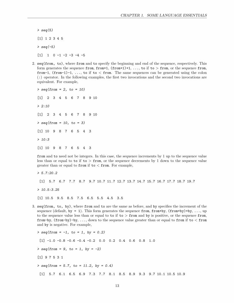
1. seq(value), where value is an integer. If value is a positive integer, seq(value) generates thesequence 1, 2, ..., value. If value is a negative integer, seq(value) generates the sequence 1, 0,..., -value. For example,
12
CHAPTER 1. SOME LANGUAGE ESSENTIALS
> seq(5)
[1] 1 2 3 4 5
> seq(-5)
[1] 1 0 -1 -2 -3 -4 -5
2. seq(from, to), where from and to specify the beginning and end of the sequence, respectively. Thisform generates the sequence from, from+1, (from+1)+1, ..., to if to > from, or the sequence from,from-1, (from-1)-1, ..., to if to < from. The same sequences can be generated using the colon(:) operator. In the following examples, the first two invocations and the second two invocations areequivalent. For example,
> seq(from = 2, to = 10)
[1] 2 3 4 5 6 7 8 9 10
> 2:10
[1] 2 3 4 5 6 7 8 9 10
> seq(from = 10, to = 3)
[1] 10 9 8 7 6 5 4 3
> 10:3
[1] 10 9 8 7 6 5 4 3
from and to need not be integers. In this case, the sequence increments by 1 up to the sequence valueless than or equal to to if to > from, or the sequence decrements by 1 down to the sequence valuegreater than or equal to from if to < from. For example,
> 5.7:20.2
[1] 5.7 6.7 7.7 8.7 9.7 10.7 11.7 12.7 13.7 14.7 15.7 16.7 17.7 18.7 19.7
> 10.5:3.25
[1] 10.5 9.5 8.5 7.5 6.5 5.5 4.5 3.5
3. seq(from, to, by), where from and to are the same as before, and by specifies the increment of thesequence (default, by = 1). This form generates the sequence from, from+by, (from+by)+by, ..., upto the sequence value less than or equal to to if to > from and by is positive, or the sequence from,from-by, (from-by)-by, ..., down to the sequence value greater than or equal to from if to < fromand by is negative. For example,
> seq(from = -1, to = 1, by = 0.2)
[1] -1.0 -0.8 -0.6 -0.4 -0.2 0.0 0.2 0.4 0.6 0.8 1.0
> seq(from = 9, to = 1, by = -2)
[1] 9 7 5 3 1
> seq(from = 5.7, to = 11.2, by = 0.4)
[1] 5.7 6.1 6.5 6.9 7.3 7.7 8.1 8.5 8.9 9.3 9.7 10.1 10.5 10.9
13
CHAPTER 1. SOME LANGUAGE ESSENTIALS
4. seq(from, to, length), where from and to are the same as before, and length specifies the desiredlength of the sequence. This form generates the sequence of length equally spaced values from fromto to. As we saw in the second form seq(from, to), if length is not specified, the default by = 1 isused. For example,
> seq(from = 2, to = 15, length = 7)
[1] 2.000000 4.166667 6.333333 8.500000 10.666667 12.833333 15.000000
NOTE: Assignment can be appropriately incorporated into any of the previous demonstrations of the c()(concatenate) and seq() functions.
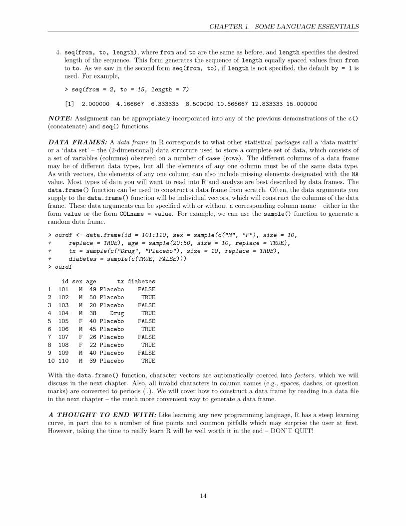
DATA FRAMES: A data frame in R corresponds to what other statistical packages call a ‘data matrix’or a ‘data set’ – the (2-dimensional) data structure used to store a complete set of data, which consists ofa set of variables (columns) observed on a number of cases (rows). The different columns of a data framemay be of different data types, but all the elements of any one column must be of the same data type.As with vectors, the elements of any one column can also include missing elements designated with the NAvalue. Most types of data you will want to read into R and analyze are best described by data frames. Thedata.frame() function can be used to construct a data frame from scratch. Often, the data arguments yousupply to the data.frame() function will be individual vectors, which will construct the columns of the dataframe. These data arguments can be specified with or without a corresponding column name – either in theform value or the form COLname = value. For example, we can use the sample() function to generate arandom data frame.
> ourdf <- data.frame(id = 101:110, sex = sample(c("M", "F"), size = 10,
+ replace = TRUE), age = sample(20:50, size = 10, replace = TRUE),
+ tx = sample(c("Drug", "Placebo"), size = 10, replace = TRUE),
+ diabetes = sample(c(TRUE, FALSE)))
> ourdf
id sex age tx diabetes1 101 M 49 Placebo FALSE2 102 M 50 Placebo TRUE3 103 M 20 Placebo FALSE4 104 M 38 Drug TRUE5 105 F 40 Placebo FALSE6 106 M 45 Placebo TRUE7 107 F 26 Placebo FALSE8 108 F 22 Placebo TRUE9 109 M 40 Placebo FALSE10 110 M 39 Placebo TRUE
With the data.frame() function, character vectors are automatically coerced into factors, which we willdiscuss in the next chapter. Also, all invalid characters in column names (e.g., spaces, dashes, or questionmarks) are converted to periods (.). We will cover how to construct a data frame by reading in a data filein the next chapter – the much more convenient way to generate a data frame.
A THOUGHT TO END WITH: Like learning any new programming language, R has a steep learningcurve, in part due to a number of fine points and common pitfalls which may surprise the user at first.However, taking the time to really learn R will be well worth it in the end – DON’T QUIT!
14

Chapter 2
Data Import and Prep
Learning objectivesTo understand how to import a delimited text file, obtain the various attributes of a read-in data set, andcustomize a data set after input.
Now that we have discussed some of the essentials of the R language, our next logical step would be toperform some analysis on an actual data set. Based on our knowledge from the first lecture, we could use thec() (‘concatenate’) and data.frame() functions to construct our data set by typing in the values of eachvariable and assigning each vector its corresponding variable name. However, in general, this plan of attackis quite impractical depending on the size of the desired data set. It also provides a perfect opportunity forerrors to creep into the data set. If the data is already recorded in some format, it’s better to be able to readit in. The way this is done depends on how the data is stored, as data sets may be found on web pages, asformatted text files, as spreadsheets, or in many other formats.
MOTIVATING DATA SET: The rest of this document will center around an example data set – arandom subset of the well known Primary Biliary Cirrhosis data set. The full data set contains the datafrom the Mayo Clinic trial in primary biliary cirrhosis (PBC) of the liver conducted between 1974 and 1984.Specifically, the trial was a randomized placebo controlled trial of the drug D-penicillamine. The randomsubset of the PBC data set that we will be using has been saved as a Microsoft Excel file (pbc.xls). Thefile contains N = 100 records (rows) and the following variables (columns):
Variable Name Variable DescriptionID Case numberFUDays Number of days between registration and the earlier of death, transplantion, or
study analysis time in July, 1986Status Status, where 0 = Censored, 1 = Censored due to liver treatment, and 2 = DeathDrug Treatment, where 1 = D-penicillamine and 2 = PlaceboAge Age in daysSex Gender, Male/FemaleAscites Presence of ascites, No/YesBili Serum bilirubin in mg/dlChol Serum cholesterol in mg/dlAlbum Albumin in gm/dlStage Histological stage of disease
MICROSOFT EXCEL FILES: Your data file is often stored as a Microsoft Excel file, but unfortunately,R can not directly read such a file. R generally wants to read in a delimited text file. Luckily, it is veryeasy to use Microsoft Excel to export your data file in a tab-delimited or comma-delimited form. You can
15
CHAPTER 2. DATA IMPORT AND PREP
then use the read.table() function, which we’ll discuss in detail, to read the exported data file into R. Youcan convert a file from Microsoft Excel to another file format by saving it with the Save As command fromthe File drop menu. Use the Save as type: drop box to choose the desired file format, such as tab-delimitedtext (.txt) or comma-delimited text (.csv). Remember, for most file formats, Excel converts only the activesheet. To convert the other sheets, switch to each sheet and save it separately.
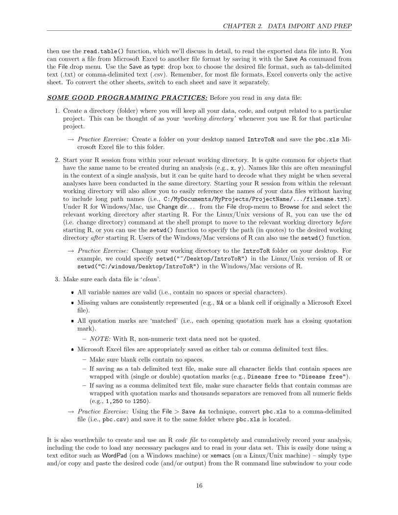
SOME GOOD PROGRAMMING PRACTICES: Before you read in any data file:
1. Create a directory (folder) where you will keep all your data, code, and output related to a particularproject. This can be thought of as your ‘working directory’ whenever you use R for that particularproject.
→ Practice Exercise: Create a folder on your desktop named IntroToR and save the pbc.xls Mi-crosoft Excel file to this folder.
2. Start your R session from within your relevant working directory. It is quite common for objects thathave the same name to be created during an analysis (e.g., x, y). Names like this are often meaningfulin the context of a single analysis, but it can be quite hard to decode what they might be when severalanalyses have been conducted in the same directory. Starting your R session from within the relevantworking directory will also allow you to easily reference the names of your data files without havingto include long path names (i.e., C:/MyDocuments/MyProjects/ProjectName/.../filename.txt).Under R for Windows/Mac, use Change dir. . . from the File drop-menu to Browse for and select therelevant working directory after starting R. For the Linux/Unix versions of R, you can use the cd(i.e. change directory) command at the shell prompt to move to the relevant working directory beforestarting R, or you can use the setwd() function to specify the path (in quotes) to the desired workingdirectory after starting R. Users of the Windows/Mac versions of R can also use the setwd() function.
→ Practice Exercise: Change your working directory to the IntroToR folder on your desktop. Forexample, we could specify setwd("~/Desktop/IntroToR") in the Linux/Unix version of R orsetwd("C:/windows/Desktop/IntroToR") in the Windows/Mac versions of R.
3. Make sure each data file is ‘clean’.
� All variable names are valid (i.e., contain no spaces or special characters).
� Missing values are consistently represented (e.g., NA or a blank cell if originally a Microsoft Excelfile).
� All quotation marks are ‘matched’ (i.e., each opening quotation mark has a closing quotationmark).
– NOTE: With R, non-numeric text data need not be quoted.
� Microsoft Excel files are appropriately saved as either tab or comma delimited text files.
– Make sure blank cells contain no spaces.– If saving as a tab delimited text file, make sure all character fields that contain spaces are
wrapped with (single or double) quotation marks (e.g., Disease free to "Disease free").– If saving as a comma delimited text file, make sure character fields that contain commas are
wrapped with quotation marks and thousands separators are removed from all numeric fields(e.g., 1,250 to 1250).
→ Practice Exercise: Using the File > Save As technique, convert pbc.xls to a comma-delimitedfile (i.e., pbc.csv) and save it to the same folder where pbc.xls is located.
It is also worthwhile to create and use an R code file to completely and cumulatively record your analysis,including the code to load any necessary packages and to read in your data set. This is easily done using atext editor such as WordPad (on a Windows machine) or xemacs (on a Linux/Unix machine) – simply typeand/or copy and paste the desired code (and/or output) from the R command line subwindow to your code
16
CHAPTER 2. DATA IMPORT AND PREP
file, and vice versa. Doing so ensures reproducible results. It also allows you to ‘cannibalize’ your code forother projects.
→ Practice Exercise: Save the Scott.IntroToR.I.R file, which contains the extracted R code from thislecture, to the same folder where pbc.xls and pbc.csv are located and open it with an appropriate texteditor.
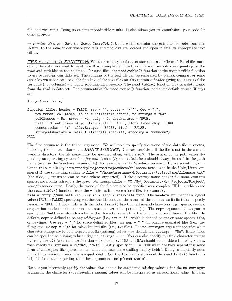
THE read.table() FUNCTION: Whether or not your data set starts out as a Microsoft Excel file, mostoften, the data you want to read into R is a simple delimited text file with records corresponding to therows and variables to the columns. For such files, the read.table() function is the most flexible functionto use to read-in your data set. The columns of the text file can be separated by blanks, commas, or someother known separator. And the first line of the text file can also contain a header giving the names of thevariables (i.e., columns) – a highly recommended practice. The read.table() function creates a data framefrom the read in data set. The arguments of the read.table() function, and their default values (if any)are:
> args(read.table)
function (file, header = FALSE, sep = "", quote = "\"'", dec = ".",row.names, col.names, as.is = !stringsAsFactors, na.strings = "NA",colClasses = NA, nrows = -1, skip = 0, check.names = TRUE,fill = !blank.lines.skip, strip.white = FALSE, blank.lines.skip = TRUE,comment.char = "#", allowEscapes = FALSE, flush = FALSE,stringsAsFactors = default.stringsAsFactors(), encoding = "unknown")
NULL
The first argument is the file= argument. We will need to specify the name of the data file in quotes,including the file extension – and DON’T FORGET , R is case sensitive. If the file is not in the currentworking directory, the file name must be specified along with its path. The syntax of the path varies de-pending on operating system, but forward slashes (/; not backslashes) should always be used in the pathname (even in the Windows version of R). For example, in the Windows version of R, use something sim-ilar to file = "C:/MyDocuments/MyProjects/ProjectName/filename.txt". And in the Unix/Linux ver-sion of R, use something similar to file = "/home/username/MyDocuments/ProjectName/filename.txt"(the tilde, ˜, expansion can be used where supported). If the directory name and/or file name containsspaces, use a backslash before the space. For example,file = "C:/My\ Documents/My\ Projects/Project\Name/filename.txt". Lastly, the name of the file can also be specified as a complete URL, in which casethe read.table() function reads the website as if it were a local file. For example,file = "http://www.math.csi.cuny.edu/UsingR/Data/whale.txt". The header= argument is a logicalvalue (TRUE or FALSE) specifying whether the file contains the names of the columns as its first line – specifyheader = TRUE if it does. Like with the data.frame() function, all invalid characters (e.g., spaces, dashes,or question marks) in the column names are converted to periods (.). The sep= argument allows you tospecify the ‘field separator character’ – the character separating the columns on each line of the file. Bydefault, sep= is defined to be any whitespace (i.e., sep = ""), which is defined as one or more spaces, tabs,or newlines. Use sep = " " for space delimited files; use sep = "," for comma-separated files (i.e., .csvfiles); and use sep = "\t" for tab-delimited files (i.e., .txt files). The na.strings= argument specifies whatcharacter strings are to be interpreted as NA (missing) values – by default, na.strings = "NA". Blank fieldscan be specified as missing values using na.strings = "". You can also specify multiple character stringsby using the c() (concatenate) function – for instance, if NA and N/A should be considered missing values,then specify na.strings = c("NA", "N/A"). Lastly, specify fill = TRUE when the file’s separator is someform of whitespace like spaces or tabs and some rows have trailing ‘empty fields’. Doing so implicitly addsblank fields when the rows have unequal length. See the Arguments section of the read.table() function’shelp file for details regarding the other arguments – help(read.table).
Note, if you incorrectly specify the values that should be considered missing values using the na.strings=argument, the character(s) representing missing values will be interpreted as an additional value. In turn,
17
CHAPTER 2. DATA IMPORT AND PREP
any numeric variables will be coerced to character fields.
→ Practice Exercise: We’re now ready to import our PBC data file using the read.table() function. Recall,the name of our file is pbc.csv, the first row does contain column names, and the columns of the delimitedfile are separated by commas (i.e., a comma-delimited file). In addition, we need to be aware that missingvalues are represented by blank cells in pbc.csv. Putting this all together,
> pbc <- read.table("pbc.csv", header = TRUE, sep = ",", na.strings = "")
→ Practice Exercise: How would you change the previous code if our pbc.xls file had been saved as a tabdelimited file with the first row containing column names and missing values represented by NA?
BE AWARE: The read.table() function can be an inefficient way to read in very large datasets. Bydefault, the read.table() function needs to read in every column as character data, and then try to figureout which variables to convert to numeric or factor. For a large dataset, this takes considerable amounts oftime and memory. The performance of the read.table() function can be improved by any of the following:(1) use the colClasses= argument to specify the classes as one of the atomic vector types (logical, integer,numeric, complex, character, or perhaps raw) for each column; (2) specify comment.char = ""; and/or (3)use the nrows= argument to give the number of rows to be read – a mild over-estimate is better than notspecifying this at all. Another alternative is to use the scan() function instead of the read.table() function.
Irregardless of how you read your data file(s) into R, if no errors are given, it is always a good practice tocheck that your data was read in correctly. An easy way to do this is to view the attributes of your read indata set. REMEMBER: In R, your read in data set has the data structure of a data frame.
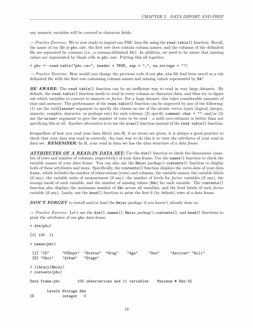
ATTRIBUTES OF A READ-IN DATA SET: Use the dim() function to check the dimensions (num-ber of rows and number of columns, respectively) of your data frame. Use the names() function to check thevariable names of your data frame. You can also use the Hmisc package’s contents() function to displayboth of these attributes and more. Specifically, the contents() function displays the meta-data of your dataframe, which includes the number of observations (rows) and columns, the variable names, the variable labels(if any), the variable units of measurement (if any), the number of levels for factor variables (if any), thestorage mode of each variable, and the number of missing values (NAs) for each variable. The contents()function also displays the maximum number of NAs across all variables, and the level labels of each factorvariable (if any). Lastly, use the head() function to print the first 6 (by default) rows of a data frame.
DON’T FORGET to install and/or load the Hmisc package if you haven’t already done so.
→ Practice Exercise: Let’s use the dim(), names(), Hmisc package’s contents(), and head() functions toprint the attributes of our pbc data frame
> dim(pbc)
[1] 100 11
> names(pbc)
[1] "ID" "FUDays" "Status" "Drug" "Age" "Sex" "Ascites" "Bili"[9] "Chol" "Album" "Stage"
> library(Hmisc)
> contents(pbc)
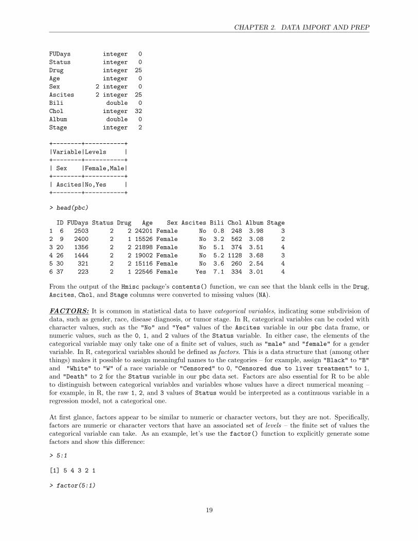
Data frame:pbc 100 observations and 11 variables Maximum # NAs:32
Levels Storage NAsID integer 0
18
CHAPTER 2. DATA IMPORT AND PREP
FUDays integer 0Status integer 0Drug integer 25Age integer 0Sex 2 integer 0Ascites 2 integer 25Bili double 0Chol integer 32Album double 0Stage integer 2
+--------+-----------+|Variable|Levels |+--------+-----------+| Sex |Female,Male|+--------+-----------+| Ascites|No,Yes |+--------+-----------+
> head(pbc)
ID FUDays Status Drug Age Sex Ascites Bili Chol Album Stage1 6 2503 2 2 24201 Female No 0.8 248 3.98 32 9 2400 2 1 15526 Female No 3.2 562 3.08 23 20 1356 2 2 21898 Female No 5.1 374 3.51 44 26 1444 2 2 19002 Female No 5.2 1128 3.68 35 30 321 2 2 15116 Female No 3.6 260 2.54 46 37 223 2 1 22546 Female Yes 7.1 334 3.01 4
From the output of the Hmisc package’s contents() function, we can see that the blank cells in the Drug,Ascites, Chol, and Stage columns were converted to missing values (NA).
FACTORS: It is common in statistical data to have categorical variables, indicating some subdivision ofdata, such as gender, race, disease diagnosis, or tumor stage. In R, categorical variables can be coded withcharacter values, such as the "No" and "Yes" values of the Ascites variable in our pbc data frame, ornumeric values, such as the 0, 1, and 2 values of the Status variable. In either case, the elements of thecategorical variable may only take one of a finite set of values, such as "male" and "female" for a gendervariable. In R, categorical variables should be defined as factors. This is a data structure that (among otherthings) makes it possible to assign meaningful names to the categories – for example, assign "Black" to "B"and "White" to "W" of a race variable or "Censored" to 0, "Censored due to liver treatment" to 1,and "Death" to 2 for the Status variable in our pbc data set. Factors are also essential for R to be ableto distinguish between categorical variables and variables whose values have a direct numerical meaning –for example, in R, the raw 1, 2, and 3 values of Status would be interpreted as a continuous variable in aregression model, not a categorical one.
At first glance, factors appear to be similar to numeric or character vectors, but they are not. Specifically,factors are numeric or character vectors that have an associated set of levels – the finite set of values thecategorical variable can take. As an example, let’s use the factor() function to explicitly generate somefactors and show this difference:
> 5:1
[1] 5 4 3 2 1
> factor(5:1)
19
CHAPTER 2. DATA IMPORT AND PREP
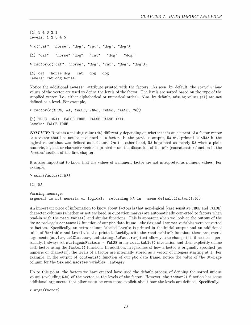
[1] 5 4 3 2 1Levels: 1 2 3 4 5
> c("cat", "horse", "dog", "cat", "dog", "dog")
[1] "cat" "horse" "dog" "cat" "dog" "dog"
> factor(c("cat", "horse", "dog", "cat", "dog", "dog"))
[1] cat horse dog cat dog dogLevels: cat dog horse
Notice the additional Levels: attribute printed with the factors. As seen, by default, the sorted uniquevalues of the vector are used to define the levels of the factor. The levels are sorted based on the type of thesupplied vector (i.e., either alphabetical or numerical order). Also, by default, missing values (NA) are notdefined as a level. For example,
> factor(c(TRUE, NA, FALSE, TRUE, FALSE, FALSE, NA))
[1] TRUE <NA> FALSE TRUE FALSE FALSE <NA>Levels: FALSE TRUE
NOTICE: R prints a missing value (NA) differently depending on whether it is an element of a factor vectoror a vector that has not been defined as a factor. In the previous output, NA was printed as <NA> in thelogical vector that was defined as a factor. On the other hand, NA is printed as merely NA when a plainnumeric, logical, or character vector is printed – see the discussion of the c() (concatenate) function in the‘Vectors’ section of the first chapter.
It is also important to know that the values of a numeric factor are not interpreted as numeric values. Forexample,
> mean(factor(1:5))
[1] NA
Warning message:argument is not numeric or logical: returning NA in: mean.default(factor(1:5))
An important piece of information to know about factors is that non-logical (case sensitive TRUE and FALSE)character columns (whether or not enclosed in quotation marks) are automatically converted to factors whenread-in with the read.table() and similar functions. This is apparent when we look at the output of theHmisc package’s contents() function of our pbc data frame – the Sex and Ascites variables were convertedto factors. Specifically, an extra column labeled Levels is printed in the initial output and an additionaltable of Variable and Levels is also printed. Luckily, with the read.table() function, there are severalarguments (as.is=, colClasses=, and stringsAsFactors=) that allow you to change this if needed – per-sonally, I always set stringsAsFactors = FALSE in my read.table() invocation and then explicitly defineeach factor using the factor() function. In addition, irregardless of how a factor is originally specified (asnumeric or character), the levels of a factor are internally stored as a vector of integers starting at 1. Forexample, in the output of contents() function of our pbc data frame, notice the value of the Storagecolumn for the Sex and Ascites variables – integer.
Up to this point, the factors we have created have used the default process of defining the sorted uniquevalues (excluding NAs) of the vector as the levels of the factor. However, the factor() function has someadditional arguments that allow us to be even more explicit about how the levels are defined. Specifically,
> args(factor)
20
CHAPTER 2. DATA IMPORT AND PREP
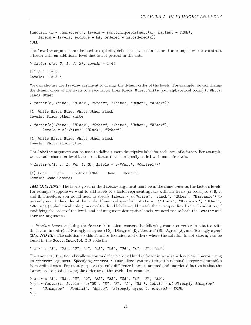
function (x = character(), levels = sort(unique.default(x), na.last = TRUE),labels = levels, exclude = NA, ordered = is.ordered(x))
NULL
The levels= argument can be used to explicitly define the levels of a factor. For example, we can constructa factor with an additional level that is not present in the data:
> factor(c(3, 3, 1, 2, 2), levels = 1:4)
[1] 3 3 1 2 2Levels: 1 2 3 4
We can also use the levels= argument to change the default order of the levels. For example, we can changethe default order of the levels of a race factor from Black, Other, White (i.e., alphabetical order) to White,Black, Other.
> factor(c("White", "Black", "Other", "White", "Other", "Black"))
[1] White Black Other White Other BlackLevels: Black Other White
> factor(c("White", "Black", "Other", "White", "Other", "Black"),
+ levels = c("White", "Black", "Other"))
[1] White Black Other White Other BlackLevels: White Black Other
The labels= argument can be used to define a more descriptive label for each level of a factor. For example,we can add character level labels to a factor that is originally coded with numeric levels.
> factor(c(1, 1, 2, NA, 1, 2), labels = c("Case", "Control"))
[1] Case Case Control <NA> Case ControlLevels: Case Control
IMPORTANT: The labels given in the labels= argument must be in the same order as the factor’s levels.For example, suppose we want to add labels to a factor representing race with the levels (in order) of W, B, O,and H. Therefore, you would need to specify labels = c("White", "Black", "Other", "Hispanic") toproperly match the order of the levels. If you had specified labels = c("Black", "Hispanic", "Other","White") (alphabetical order), none of the level labels would match the corresponding levels. In addition, ifmodifying the order of the levels and defining more descriptive labels, we need to use both the levels= andlabels= arguments.
→ Practice Exercise: Using the factor() function, convert the following character vector to a factor withthe levels (in order) of ‘Strongly disagree’ (SD), ‘Disagree’ (D), ‘Neutral’ (N), ‘Agree’ (A), and ‘Strongly agree’(SA). NOTE: The solution to this Practice Exercise, and others where the solution is not shown, can befound in the Scott.IntroToR.I.R code file.
> x <- c("A", "SA", "D", "D", "SA", "SA", "SA", "A", "N", "SD")
The factor() function also allows you to define a special kind of factor in which the levels are ordered, usingits ordered= argument. Specifying ordered = TRUE allows you to distinguish nominal categorical variablesfrom ordinal ones. For most purposes the only difference between ordered and unordered factors is that theformer are printed showing the ordering of the levels. For example,
> x <- c("A", "SA", "D", "D", "SA", "SA", "SA", "A", "N", "SD")
> y <- factor(x, levels = c("SD", "D", "N", "A", "SA"), labels = c("Strongly disagree",
+ "Disagree", "Neutral", "Agree", "Strongly agree"), ordered = TRUE)
> y
21

CHAPTER 2. DATA IMPORT AND PREP
[1] Agree Strongly agree Disagree Disagree[5] Strongly agree Strongly agree Strongly agree Agree[9] Neutral Strongly disagreeLevels: Strongly disagree < Disagree < Neutral < Agree < Strongly agree
As you can see, when printed, the levels of an ordered factor display the ordering relation (<) between thelevels of the factor. This can also be useful when you wish to compare the levels of an ordered factor. Forexample,
> y < "Neutral"
[1] FALSE FALSE TRUE TRUE FALSE FALSE FALSE FALSE FALSE TRUE
We’ll discuss comparison operators, like <, in the second document.
Once a factor has been created, the levels() function can be used to return, reorder, and/or redefine itslevels (including assigning new level labels, defining new levels, and collapsing existing levels into new levels).To redefine the levels of a factor using the levels() function, we can specify a named list specifying how toredefine/reorder the levels (i.e., list(NEWlevel = "OLDlevel")). The list can also specify new levels. Forexample,
> test <- factor(c("positive", "negative", "negative"))
> levels(test)
[1] "negative" "positive"
> levels(test) <- list(positive = "positive", negative = "negative")
> levels(test)
[1] "positive" "negative"
> levels(test) <- list(Positive = "positive", Negative = "negative")
> test
[1] Positive Negative NegativeLevels: Positive Negative
> levels(test) <- list(Undetermined = "Undetermined", Positive = "Positive",
+ Negative = "Negative")
> test
[1] Positive Negative NegativeLevels: Undetermined Positive Negative
> levels(test) <- list(Combined = c("Undetermined", "Positive"), Negative = "Negative")
> test
[1] Combined Negative NegativeLevels: Combined Negative
As a side note, when manipulating factors, it is always a good idea to generate a frequency table of the factorboth before and after you modify its levels and/or labels – see the table() function, which is explained inthe ‘Tables of categorical variables’ section of the ‘Descriptive Statistics’ chapter.
→ Practice Exercise: Using the levels() function, collapse the five-level factor you created in the previouspractice exercise to a three level factor with the levels of ‘Disagree’ (strongly disagree or disagree), ‘Neutral’,and ‘Agree’ (agree or strongly agree).
22
CHAPTER 2. DATA IMPORT AND PREP
CUSTOMIZING DATA SETS AFTER INPUT: Now that we’ve read in our data file and have en-sured it was read in correctly, we may want to make some modifications. There are many ways you cancustomize a data frame, including renaming variables, adding new variables, deleting variables, adding orchanging the levels of a factor variable, adding or changing variable labels, and/or adding or changing theunits of measurement of a variable. There are many functions that are useful in performing some of themodifications mentioned and we could make many of our desired modifications using individual functioninvocations, but there is an easier way using the Hmisc package’s upData() function. The Hmisc package’supData() function provides a unified framework for updating a data frame. It accomplishes the following,listed in the order in which the changes are executed:
1. Optionally changes names of variables to lower case.
2. Renames variables.
3. Adds new variables.
4. Recomputes existing variables from the original variables and/or from other variables in the data frame.
5. Changes the storage mode of variables to the most efficient mode.
6. Drops (deletes) variables.
7. Adds, changes, and combines levels of factor variables.
8. Adds or changes variable labels.
9. Adds or changes variable units.
Making any of these changes upfront will allow you take full advantage of any of them during your analyses.For example, many functions will automatically print variable labels and units as part of their output, makinginterpretation of the results a lot easier. Using the Hmisc package’s upData() function also allows you to de-fine all of the modifications in one function invocation, making all of the modifications much easier to manage.
The arguments of the Hmisc package’s upData() function are (remember, we’ve already loaded the Hmiscpackage)
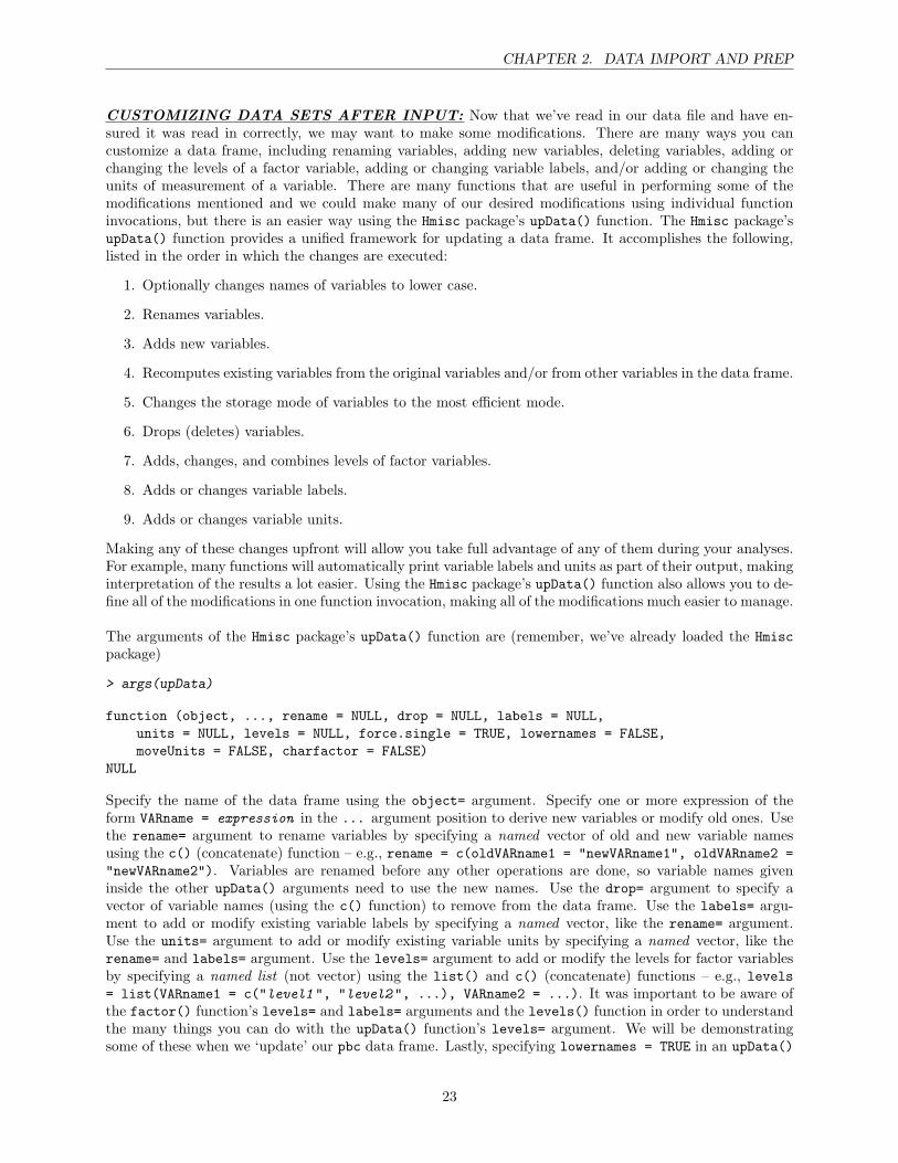
> args(upData)
function (object, ..., rename = NULL, drop = NULL, labels = NULL,units = NULL, levels = NULL, force.single = TRUE, lowernames = FALSE,moveUnits = FALSE, charfactor = FALSE)
NULL
Specify the name of the data frame using the object= argument. Specify one or more expression of theform VARname = expression in the ... argument position to derive new variables or modify old ones. Usethe rename= argument to rename variables by specifying a named vector of old and new variable namesusing the c() (concatenate) function – e.g., rename = c(oldVARname1 = "newVARname1", oldVARname2 ="newVARname2"). Variables are renamed before any other operations are done, so variable names giveninside the other upData() arguments need to use the new names. Use the drop= argument to specify avector of variable names (using the c() function) to remove from the data frame. Use the labels= argu-ment to add or modify existing variable labels by specifying a named vector, like the rename= argument.Use the units= argument to add or modify existing variable units by specifying a named vector, like therename= and labels= argument. Use the levels= argument to add or modify the levels for factor variablesby specifying a named list (not vector) using the list() and c() (concatenate) functions – e.g., levels= list(VARname1 = c("level1 ", "level2 ", ...), VARname2 = ...). It was important to be aware ofthe factor() function’s levels= and labels= arguments and the levels() function in order to understandthe many things you can do with the upData() function’s levels= argument. We will be demonstratingsome of these when we ‘update’ our pbc data frame. Lastly, specifying lowernames = TRUE in an upData()
23
CHAPTER 2. DATA IMPORT AND PREP
function invocation will coerce all the column names to lower-case.
When you invoke the Hmisc package’s upData() function, you can either overwrite the original data frameby assigning the function invocation to original data frame (e.g., pbc <- upData(pbc, ...)), or you canassign the function invocation to a new data frame (e.g., new.pbc <- upData(pbc, ...)).
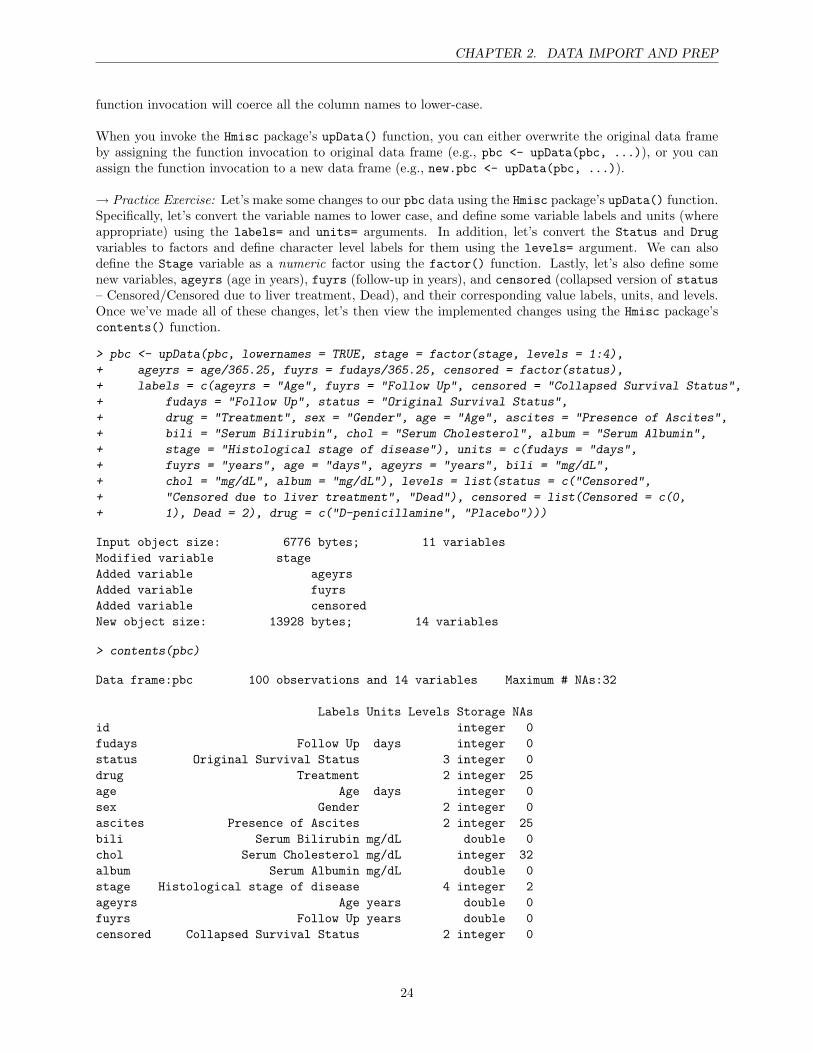
→ Practice Exercise: Let’s make some changes to our pbc data using the Hmisc package’s upData() function.Specifically, let’s convert the variable names to lower case, and define some variable labels and units (whereappropriate) using the labels= and units= arguments. In addition, let’s convert the Status and Drugvariables to factors and define character level labels for them using the levels= argument. We can alsodefine the Stage variable as a numeric factor using the factor() function. Lastly, let’s also define somenew variables, ageyrs (age in years), fuyrs (follow-up in years), and censored (collapsed version of status– Censored/Censored due to liver treatment, Dead), and their corresponding value labels, units, and levels.Once we’ve made all of these changes, let’s then view the implemented changes using the Hmisc package’scontents() function.
> pbc <- upData(pbc, lowernames = TRUE, stage = factor(stage, levels = 1:4),
+ ageyrs = age/365.25, fuyrs = fudays/365.25, censored = factor(status),
+ labels = c(ageyrs = "Age", fuyrs = "Follow Up", censored = "Collapsed Survival Status",
+ fudays = "Follow Up", status = "Original Survival Status",
+ drug = "Treatment", sex = "Gender", age = "Age", ascites = "Presence of Ascites",
+ bili = "Serum Bilirubin", chol = "Serum Cholesterol", album = "Serum Albumin",
+ stage = "Histological stage of disease"), units = c(fudays = "days",
+ fuyrs = "years", age = "days", ageyrs = "years", bili = "mg/dL",
+ chol = "mg/dL", album = "mg/dL"), levels = list(status = c("Censored",
+ "Censored due to liver treatment", "Dead"), censored = list(Censored = c(0,
+ 1), Dead = 2), drug = c("D-penicillamine", "Placebo")))
Input object size: 6776 bytes; 11 variablesModified variable stageAdded variable ageyrsAdded variable fuyrsAdded variable censoredNew object size: 13928 bytes; 14 variables
> contents(pbc)
Data frame:pbc 100 observations and 14 variables Maximum # NAs:32
Labels Units Levels Storage NAsid integer 0fudays Follow Up days integer 0status Original Survival Status 3 integer 0drug Treatment 2 integer 25age Age days integer 0sex Gender 2 integer 0ascites Presence of Ascites 2 integer 25bili Serum Bilirubin mg/dL double 0chol Serum Cholesterol mg/dL integer 32album Serum Albumin mg/dL double 0stage Histological stage of disease 4 integer 2ageyrs Age years double 0fuyrs Follow Up years double 0censored Collapsed Survival Status 2 integer 0
24
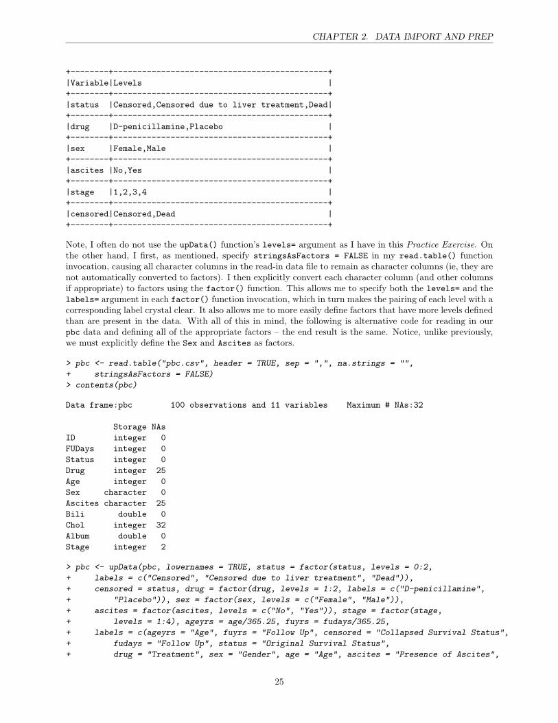
CHAPTER 2. DATA IMPORT AND PREP
+--------+---------------------------------------------+|Variable|Levels |+--------+---------------------------------------------+|status |Censored,Censored due to liver treatment,Dead|+--------+---------------------------------------------+|drug |D-penicillamine,Placebo |+--------+---------------------------------------------+|sex |Female,Male |+--------+---------------------------------------------+|ascites |No,Yes |+--------+---------------------------------------------+|stage |1,2,3,4 |+--------+---------------------------------------------+|censored|Censored,Dead |+--------+---------------------------------------------+
Note, I often do not use the upData() function’s levels= argument as I have in this Practice Exercise. Onthe other hand, I first, as mentioned, specify stringsAsFactors = FALSE in my read.table() functioninvocation, causing all character columns in the read-in data file to remain as character columns (ie, they arenot automatically converted to factors). I then explicitly convert each character column (and other columnsif appropriate) to factors using the factor() function. This allows me to specify both the levels= and thelabels= argument in each factor() function invocation, which in turn makes the pairing of each level with acorresponding label crystal clear. It also allows me to more easily define factors that have more levels definedthan are present in the data. With all of this in mind, the following is alternative code for reading in ourpbc data and defining all of the appropriate factors – the end result is the same. Notice, unlike previously,we must explicitly define the Sex and Ascites as factors.
> pbc <- read.table("pbc.csv", header = TRUE, sep = ",", na.strings = "",
+ stringsAsFactors = FALSE)
> contents(pbc)
Data frame:pbc 100 observations and 11 variables Maximum # NAs:32
Storage NAsID integer 0FUDays integer 0Status integer 0Drug integer 25Age integer 0Sex character 0Ascites character 25Bili double 0Chol integer 32Album double 0Stage integer 2
> pbc <- upData(pbc, lowernames = TRUE, status = factor(status, levels = 0:2,
+ labels = c("Censored", "Censored due to liver treatment", "Dead")),
+ censored = status, drug = factor(drug, levels = 1:2, labels = c("D-penicillamine",
+ "Placebo")), sex = factor(sex, levels = c("Female", "Male")),
+ ascites = factor(ascites, levels = c("No", "Yes")), stage = factor(stage,
+ levels = 1:4), ageyrs = age/365.25, fuyrs = fudays/365.25,
+ labels = c(ageyrs = "Age", fuyrs = "Follow Up", censored = "Collapsed Survival Status",
+ fudays = "Follow Up", status = "Original Survival Status",
+ drug = "Treatment", sex = "Gender", age = "Age", ascites = "Presence of Ascites",
25
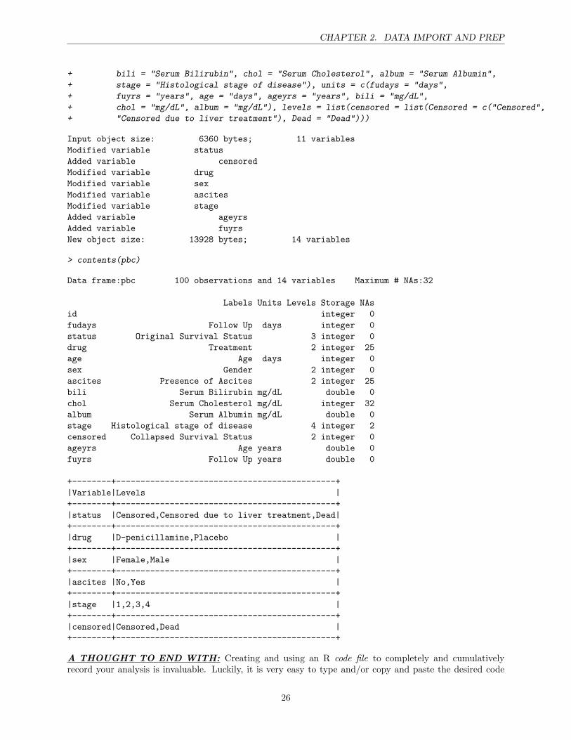
CHAPTER 2. DATA IMPORT AND PREP
+ bili = "Serum Bilirubin", chol = "Serum Cholesterol", album = "Serum Albumin",
+ stage = "Histological stage of disease"), units = c(fudays = "days",
+ fuyrs = "years", age = "days", ageyrs = "years", bili = "mg/dL",
+ chol = "mg/dL", album = "mg/dL"), levels = list(censored = list(Censored = c("Censored",
+ "Censored due to liver treatment"), Dead = "Dead")))
Input object size: 6360 bytes; 11 variablesModified variable statusAdded variable censoredModified variable drugModified variable sexModified variable ascitesModified variable stageAdded variable ageyrsAdded variable fuyrsNew object size: 13928 bytes; 14 variables
> contents(pbc)
Data frame:pbc 100 observations and 14 variables Maximum # NAs:32
Labels Units Levels Storage NAsid integer 0fudays Follow Up days integer 0status Original Survival Status 3 integer 0drug Treatment 2 integer 25age Age days integer 0sex Gender 2 integer 0ascites Presence of Ascites 2 integer 25bili Serum Bilirubin mg/dL double 0chol Serum Cholesterol mg/dL integer 32album Serum Albumin mg/dL double 0stage Histological stage of disease 4 integer 2censored Collapsed Survival Status 2 integer 0ageyrs Age years double 0fuyrs Follow Up years double 0
+--------+---------------------------------------------+|Variable|Levels |+--------+---------------------------------------------+|status |Censored,Censored due to liver treatment,Dead|+--------+---------------------------------------------+|drug |D-penicillamine,Placebo |+--------+---------------------------------------------+|sex |Female,Male |+--------+---------------------------------------------+|ascites |No,Yes |+--------+---------------------------------------------+|stage |1,2,3,4 |+--------+---------------------------------------------+|censored|Censored,Dead |+--------+---------------------------------------------+
A THOUGHT TO END WITH: Creating and using an R code file to completely and cumulativelyrecord your analysis is invaluable. Luckily, it is very easy to type and/or copy and paste the desired code
26
CHAPTER 2. DATA IMPORT AND PREP
(and/or output) from the R command line subwindow to your code file, and vice versa. If you are on a Win-dows machine, I would recommend formatting your code and output using the Courier New (monospace)font, which is very similar to what is used in R.
Even though it is very easy create a code file, it is imperative that you try make your code files well readableand as much self-explaining as possible. This includes
� indenting and using spaces appropriately;
� explicitly specifying function arguments by their ARGname tag;
� wrapping long lines of code by explicitly breaking long expressions;
– Explicitly break long expression by inserting a newline (i.e., a carriage return) after a knownseparator that is syntactically relevant. In particular, break a long expression after a commaseparating the arguments of a function; after a logical operator (& = ‘and’ or | = ‘or’) within alogical statement; or after a plus sign (+) within a formula statement (e.g., Y ~ X1 + X2).
� and adding copious comments to your code.
– Any text following a # on the command line, to the end of the line, is taken as a ‘comment’ andignored by R. Comments can be put almost anywhere, except inside quoted strings, and withinthe argument list of a function definition. For example,
> 175*(8/5) # convert 175 miles to kms[1] 280
See the Scott.IntroToR.I.R code file for an illustration of all of these tips. You’ll notice that the Scott.IntroToR.I.Rcode file includes the R code to set the working directory (setwd()) and load any necessary packages(library()).
When all your R code is collected and recorded in a code file, the results can be reproduced at any time. Inaddition, if your R code is stored in an external file, say Rcode.R in the current working directory, all of theexpressions can be executed at any time in an R session with the expression source("Rcode.R"). This isextremely useful if you have defined your own function (as we will discuss in more detail) in an external fileand wish to source the function. The source() function also has a verbose= argument, which (when set toTRUE) will cause each expression and additional diagnostics to be printed during the parsing and evaluationof the input file.
27
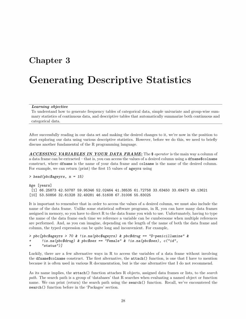
Chapter 3
Generating Descriptive Statistics
Learning objectiveTo understand how to generate frequency tables of categorical data, simple univariate and group-wise sum-mary statistics of continuous data, and descriptive tables that automatically summarize both continuous andcategorical data.
After successfully reading in our data set and making the desired changes to it, we’re now in the position tostart exploring our data using various descriptive statistics. However, before we do this, we need to brieflydiscuss another fundamental of the R programming language.
ACCESSING VARIABLES IN YOUR DATA FRAME: The $ operator is the main way a column ofa data frame can be extracted – that is, you can access the values of a desired column using a dfname$colnameconstruct, where dfname is the name of your data frame and colname is the name of the desired column.For example, we can return (print) the first 15 values of ageyrs using
> head(pbc$ageyrs, n = 15)
Age [years][1] 66.25873 42.50787 59.95346 52.02464 41.38535 61.72758 33.63450 33.69473 49.13621[10] 53.50856 32.61328 32.49281 46.51608 67.31006 55.83025
It is important to remember that in order to access the values of a desired column, we must also include thename of the data frame. Unlike some statistical software programs, in R, you can have many data framesassigned in memory, so you have to direct R to the data frame you wish to use. Unfortunately, having to typethe name of the data frame each time we reference a variable can be cumbersome when multiple referencesare performed. And, as you can imagine, depending on the length of the name of both the data frame andcolumn, the typed expression can be quite long and inconvenient. For example,
> pbc[pbc$ageyrs > 70 & !is.na(pbc$ageyrs) & pbc$drug == "D-penicillamine" &
+ !is.na(pbc$drug) & pbc$sex == "Female" & !is.na(pbc$sex), c("id",
+ "status")]
Luckily, there are a few alternative ways in R to access the variables of a data frame without involvingthe dfname$colname construct. The first alternative, the attach() function, is one that I have to mentionbecause it is often used in various R documentation, but is the one alternative that I do not recommend.
As its name implies, the attach() function attaches R objects, assigned data frames or lists, to the searchpath. The search path is a group of ‘databases’ that R searches when evaluating a named object or functionname. We can print (return) the search path using the search() function. Recall, we’ve encountered thesearch() function before in the ‘Packages’ section.
28
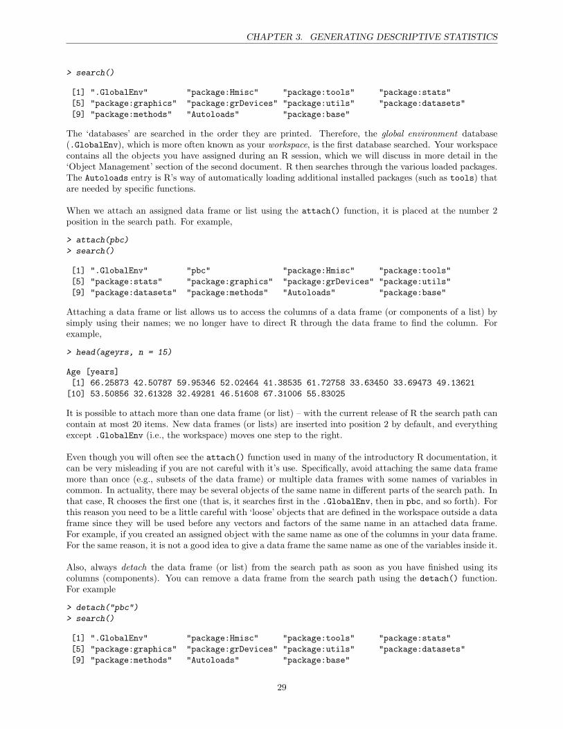
CHAPTER 3. GENERATING DESCRIPTIVE STATISTICS
> search()
[1] ".GlobalEnv" "package:Hmisc" "package:tools" "package:stats"[5] "package:graphics" "package:grDevices" "package:utils" "package:datasets"[9] "package:methods" "Autoloads" "package:base"
The ‘databases’ are searched in the order they are printed. Therefore, the global environment database(.GlobalEnv), which is more often known as your workspace, is the first database searched. Your workspacecontains all the objects you have assigned during an R session, which we will discuss in more detail in the‘Object Management’ section of the second document. R then searches through the various loaded packages.The Autoloads entry is R’s way of automatically loading additional installed packages (such as tools) thatare needed by specific functions.
When we attach an assigned data frame or list using the attach() function, it is placed at the number 2position in the search path. For example,
> attach(pbc)
> search()
[1] ".GlobalEnv" "pbc" "package:Hmisc" "package:tools"[5] "package:stats" "package:graphics" "package:grDevices" "package:utils"[9] "package:datasets" "package:methods" "Autoloads" "package:base"
Attaching a data frame or list allows us to access the columns of a data frame (or components of a list) bysimply using their names; we no longer have to direct R through the data frame to find the column. Forexample,
> head(ageyrs, n = 15)
Age [years][1] 66.25873 42.50787 59.95346 52.02464 41.38535 61.72758 33.63450 33.69473 49.13621[10] 53.50856 32.61328 32.49281 46.51608 67.31006 55.83025
It is possible to attach more than one data frame (or list) – with the current release of R the search path cancontain at most 20 items. New data frames (or lists) are inserted into position 2 by default, and everythingexcept .GlobalEnv (i.e., the workspace) moves one step to the right.
Even though you will often see the attach() function used in many of the introductory R documentation, itcan be very misleading if you are not careful with it’s use. Specifically, avoid attaching the same data framemore than once (e.g., subsets of the data frame) or multiple data frames with some names of variables incommon. In actuality, there may be several objects of the same name in different parts of the search path. Inthat case, R chooses the first one (that is, it searches first in the .GlobalEnv, then in pbc, and so forth). Forthis reason you need to be a little careful with ‘loose’ objects that are defined in the workspace outside a dataframe since they will be used before any vectors and factors of the same name in an attached data frame.For example, if you created an assigned object with the same name as one of the columns in your data frame.For the same reason, it is not a good idea to give a data frame the same name as one of the variables inside it.
Also, always detach the data frame (or list) from the search path as soon as you have finished using itscolumns (components). You can remove a data frame from the search path using the detach() function.For example
> detach("pbc")
> search()
[1] ".GlobalEnv" "package:Hmisc" "package:tools" "package:stats"[5] "package:graphics" "package:grDevices" "package:utils" "package:datasets"[9] "package:methods" "Autoloads" "package:base"
29
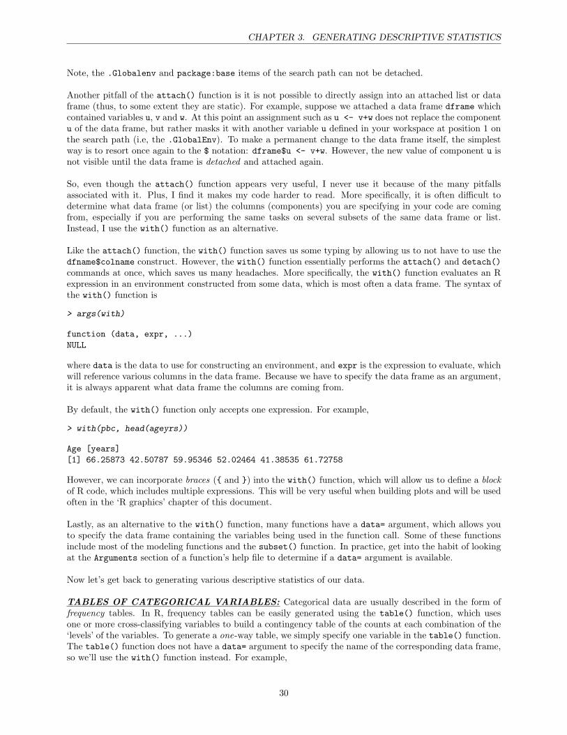
CHAPTER 3. GENERATING DESCRIPTIVE STATISTICS
Note, the .Globalenv and package:base items of the search path can not be detached.
Another pitfall of the attach() function is it is not possible to directly assign into an attached list or dataframe (thus, to some extent they are static). For example, suppose we attached a data frame dframe whichcontained variables u, v and w. At this point an assignment such as u <- v+w does not replace the componentu of the data frame, but rather masks it with another variable u defined in your workspace at position 1 onthe search path (i.e, the .GlobalEnv). To make a permanent change to the data frame itself, the simplestway is to resort once again to the $ notation: dframe$u <- v+w. However, the new value of component u isnot visible until the data frame is detached and attached again.
So, even though the attach() function appears very useful, I never use it because of the many pitfallsassociated with it. Plus, I find it makes my code harder to read. More specifically, it is often difficult todetermine what data frame (or list) the columns (components) you are specifying in your code are comingfrom, especially if you are performing the same tasks on several subsets of the same data frame or list.Instead, I use the with() function as an alternative.
Like the attach() function, the with() function saves us some typing by allowing us to not have to use thedfname$colname construct. However, the with() function essentially performs the attach() and detach()commands at once, which saves us many headaches. More specifically, the with() function evaluates an Rexpression in an environment constructed from some data, which is most often a data frame. The syntax ofthe with() function is
> args(with)
function (data, expr, ...)NULL
where data is the data to use for constructing an environment, and expr is the expression to evaluate, whichwill reference various columns in the data frame. Because we have to specify the data frame as an argument,it is always apparent what data frame the columns are coming from.
By default, the with() function only accepts one expression. For example,
> with(pbc, head(ageyrs))
Age [years][1] 66.25873 42.50787 59.95346 52.02464 41.38535 61.72758
However, we can incorporate braces ({ and }) into the with() function, which will allow us to define a blockof R code, which includes multiple expressions. This will be very useful when building plots and will be usedoften in the ‘R graphics’ chapter of this document.
Lastly, as an alternative to the with() function, many functions have a data= argument, which allows youto specify the data frame containing the variables being used in the function call. Some of these functionsinclude most of the modeling functions and the subset() function. In practice, get into the habit of lookingat the Arguments section of a function’s help file to determine if a data= argument is available.
Now let’s get back to generating various descriptive statistics of our data.
TABLES OF CATEGORICAL VARIABLES: Categorical data are usually described in the form offrequency tables. In R, frequency tables can be easily generated using the table() function, which usesone or more cross-classifying variables to build a contingency table of the counts at each combination of the‘levels’ of the variables. To generate a one-way table, we simply specify one variable in the table() function.The table() function does not have a data= argument to specify the name of the corresponding data frame,so we’ll use the with() function instead. For example,
30
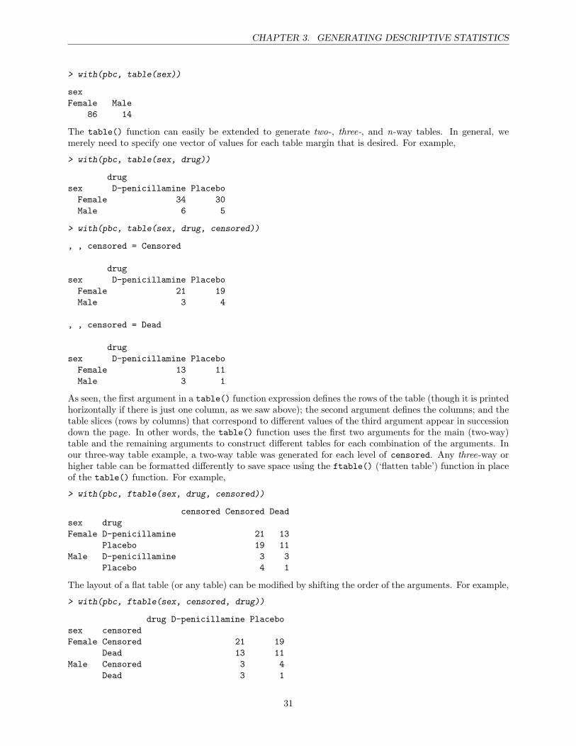
CHAPTER 3. GENERATING DESCRIPTIVE STATISTICS
> with(pbc, table(sex))
sexFemale Male
86 14
The table() function can easily be extended to generate two-, three-, and n-way tables. In general, wemerely need to specify one vector of values for each table margin that is desired. For example,
> with(pbc, table(sex, drug))
drugsex D-penicillamine PlaceboFemale 34 30Male 6 5
> with(pbc, table(sex, drug, censored))
, , censored = Censored
drugsex D-penicillamine PlaceboFemale 21 19Male 3 4
, , censored = Dead
drugsex D-penicillamine PlaceboFemale 13 11Male 3 1
As seen, the first argument in a table() function expression defines the rows of the table (though it is printedhorizontally if there is just one column, as we saw above); the second argument defines the columns; and thetable slices (rows by columns) that correspond to different values of the third argument appear in successiondown the page. In other words, the table() function uses the first two arguments for the main (two-way)table and the remaining arguments to construct different tables for each combination of the arguments. Inour three-way table example, a two-way table was generated for each level of censored. Any three-way orhigher table can be formatted differently to save space using the ftable() (‘flatten table’) function in placeof the table() function. For example,
> with(pbc, ftable(sex, drug, censored))
censored Censored Deadsex drugFemale D-penicillamine 21 13
Placebo 19 11Male D-penicillamine 3 3
Placebo 4 1
The layout of a flat table (or any table) can be modified by shifting the order of the arguments. For example,
> with(pbc, ftable(sex, censored, drug))
drug D-penicillamine Placebosex censoredFemale Censored 21 19
Dead 13 11Male Censored 3 4
Dead 3 1
31
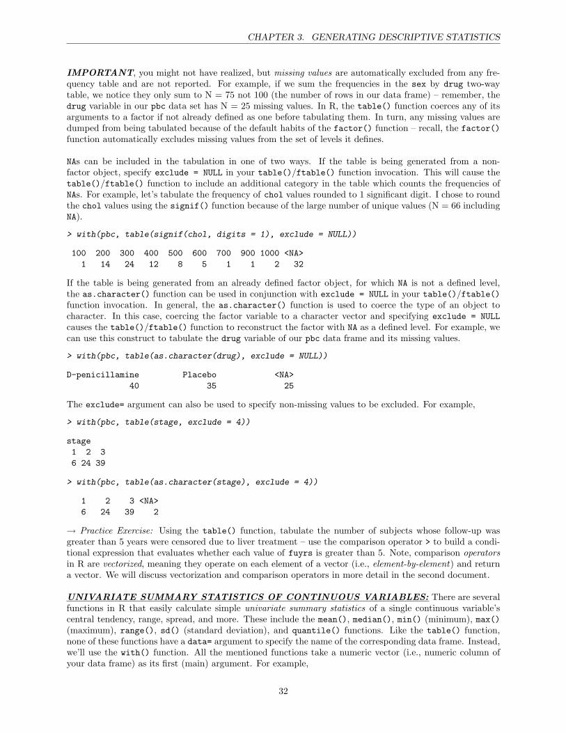
CHAPTER 3. GENERATING DESCRIPTIVE STATISTICS
IMPORTANT, you might not have realized, but missing values are automatically excluded from any fre-quency table and are not reported. For example, if we sum the frequencies in the sex by drug two-waytable, we notice they only sum to N = 75 not 100 (the number of rows in our data frame) – remember, thedrug variable in our pbc data set has N = 25 missing values. In R, the table() function coerces any of itsarguments to a factor if not already defined as one before tabulating them. In turn, any missing values aredumped from being tabulated because of the default habits of the factor() function – recall, the factor()function automatically excludes missing values from the set of levels it defines.
NAs can be included in the tabulation in one of two ways. If the table is being generated from a non-factor object, specify exclude = NULL in your table()/ftable() function invocation. This will cause thetable()/ftable() function to include an additional category in the table which counts the frequencies ofNAs. For example, let’s tabulate the frequency of chol values rounded to 1 significant digit. I chose to roundthe chol values using the signif() function because of the large number of unique values (N = 66 includingNA).
> with(pbc, table(signif(chol, digits = 1), exclude = NULL))
100 200 300 400 500 600 700 900 1000 <NA>1 14 24 12 8 5 1 1 2 32
If the table is being generated from an already defined factor object, for which NA is not a defined level,the as.character() function can be used in conjunction with exclude = NULL in your table()/ftable()function invocation. In general, the as.character() function is used to coerce the type of an object tocharacter. In this case, coercing the factor variable to a character vector and specifying exclude = NULLcauses the table()/ftable() function to reconstruct the factor with NA as a defined level. For example, wecan use this construct to tabulate the drug variable of our pbc data frame and its missing values.
> with(pbc, table(as.character(drug), exclude = NULL))
D-penicillamine Placebo <NA>40 35 25
The exclude= argument can also be used to specify non-missing values to be excluded. For example,
> with(pbc, table(stage, exclude = 4))
stage1 2 36 24 39
> with(pbc, table(as.character(stage), exclude = 4))
1 2 3 <NA>6 24 39 2
→ Practice Exercise: Using the table() function, tabulate the number of subjects whose follow-up wasgreater than 5 years were censored due to liver treatment – use the comparison operator > to build a condi-tional expression that evaluates whether each value of fuyrs is greater than 5. Note, comparison operatorsin R are vectorized, meaning they operate on each element of a vector (i.e., element-by-element) and returna vector. We will discuss vectorization and comparison operators in more detail in the second document.
UNIVARIATE SUMMARY STATISTICS OF CONTINUOUS VARIABLES: There are severalfunctions in R that easily calculate simple univariate summary statistics of a single continuous variable’scentral tendency, range, spread, and more. These include the mean(), median(), min() (minimum), max()(maximum), range(), sd() (standard deviation), and quantile() functions. Like the table() function,none of these functions have a data= argument to specify the name of the corresponding data frame. Instead,we’ll use the with() function. All the mentioned functions take a numeric vector (i.e., numeric column ofyour data frame) as its first (main) argument. For example,
32
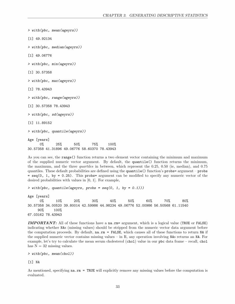
CHAPTER 3. GENERATING DESCRIPTIVE STATISTICS
> with(pbc, mean(ageyrs))
[1] 49.92134
> with(pbc, median(ageyrs))
[1] 49.06776
> with(pbc, min(ageyrs))
[1] 30.57358
> with(pbc, max(ageyrs))
[1] 78.43943
> with(pbc, range(ageyrs))
[1] 30.57358 78.43943
> with(pbc, sd(ageyrs))
[1] 11.89152
> with(pbc, quantile(ageyrs))
Age [years]0% 25% 50% 75% 100%
30.57358 41.31896 49.06776 58.60370 78.43943
As you can see, the range() function returns a two element vector containing the minimum and maximumof the supplied numeric vector argument. By default, the quantile() function returns the minimum,the maximum, and the three quartiles in between, which represent the 0.25, 0.50 (ie, median), and 0.75quantiles. These default probabilities are defined using the quantile() function’s probs= argument – probs= seq(0, 1, by = 0.25). This probs= argument can be modified to specify any numeric vector of thedesired probabilities with values in [0, 1]. For example,
> with(pbc, quantile(ageyrs, probs = seq(0, 1, by = 0.1)))
Age [years]0% 10% 20% 30% 40% 50% 60% 70% 80%
30.57358 34.00520 39.80014 42.59986 44.98234 49.06776 52.00986 56.50568 61.1154090% 100%
67.03162 78.43943
IMPORTANT: All of these functions have a na.rm= argument, which is a logical value (TRUE or FALSE)indicating whether NAs (missing values) should be stripped from the numeric vector data argument beforethe computation proceeds. By default, na.rm = FALSE, which causes all of these functions to return NA ifthe supplied numeric vector contains missing values – in R, any operation involving NAs returns an NA. Forexample, let’s try to calculate the mean serum cholesterol (chol) value in our pbc data frame – recall, cholhas N = 32 missing values.
> with(pbc, mean(chol))
[1] NA
As mentioned, specifying na.rm = TRUE will explicitly remove any missing values before the computation isevaluated.
33

CHAPTER 3. GENERATING DESCRIPTIVE STATISTICS
> with(pbc, mean(chol, na.rm = TRUE))
[1] 381.6176
There are many other basic statistics functions in R that have a similar na.rm= argument, but only some havea default value of TRUE. In addition, many functions have other na.X= arguments that dictate how missingvalues should be treated. For example, the lm() (linear model) function has a na.action= argument thatis specified as "na.fail", "na.omit", or "na.exclude". Make sure you look in the function’s help file toensure any missing values are handled correctly.
→ Practice Exercise: Use the mean(), and sd() functions to calculate the lower- and upper-limits of a 95%confidence interval around the mean of age (in years).
MORE ON MISSING VALUES: The following results may seem surprising. Note, arithmetic, compar-ison, and logic operators in R, which we will discuss in more detail in the second document, are vectorized,meaning they operate on each element of a vector (i.e., element-by-element).
> x <- c(9, 5, 12, NA, 2, NA, NA, 1)
> x + 5
[1] 14 10 17 NA 7 NA NA 6
> x > 2
[1] TRUE TRUE TRUE NA FALSE NA NA FALSE
> x == NA
[1] NA NA NA NA NA NA NA NA
In general, any operator (arithmetic, comparison, or logical) performed on an NA returns an NA. Therefore,using x == NA to test whether an element is equal to NA does not work. Instead, you must use the is.na()function, which returns a logical vector that indicates if each element is missing (NA). For example (the ! =‘not’),
> is.na(x)
[1] FALSE FALSE FALSE TRUE FALSE TRUE TRUE FALSE
> x > 2 & !is.na(x)
[1] TRUE TRUE TRUE FALSE FALSE FALSE FALSE FALSE
Missing values (NAs) can cause problems in a number of functions. It is always a good idea to look at anindividual function’s help file to determine how it will handle NAs.
→ Practice Exercise: Use the is.na() and table() functions to tabulate the number of missing ascitesvalues.
GROUP-WISE SUMMARY STATISTICS OF CONTINUOUS VARIABLES: Up to this pointwe have generated univariate summary statistics of single continuous variables ignoring any other possibleclassifying categorical variables. However, you will often want to generate summary statistics of continuousvariables at each level of various categorical ones, or at each combination of several categorical variables.Such summaries are often referred to as group-wise summary statistics. Like univariate summary statistics,there are many functions in R that can be used to generate group-wise summary statistics. However, wewill only cover the Hmisc package’s summary.formula() function in this document. The Hmisc package’ssummary.formula() function works from three main arguments: the formula=, method=, and data= argu-ments. In general, the formula= argument specifies the continuous variable you would like to summarize
34
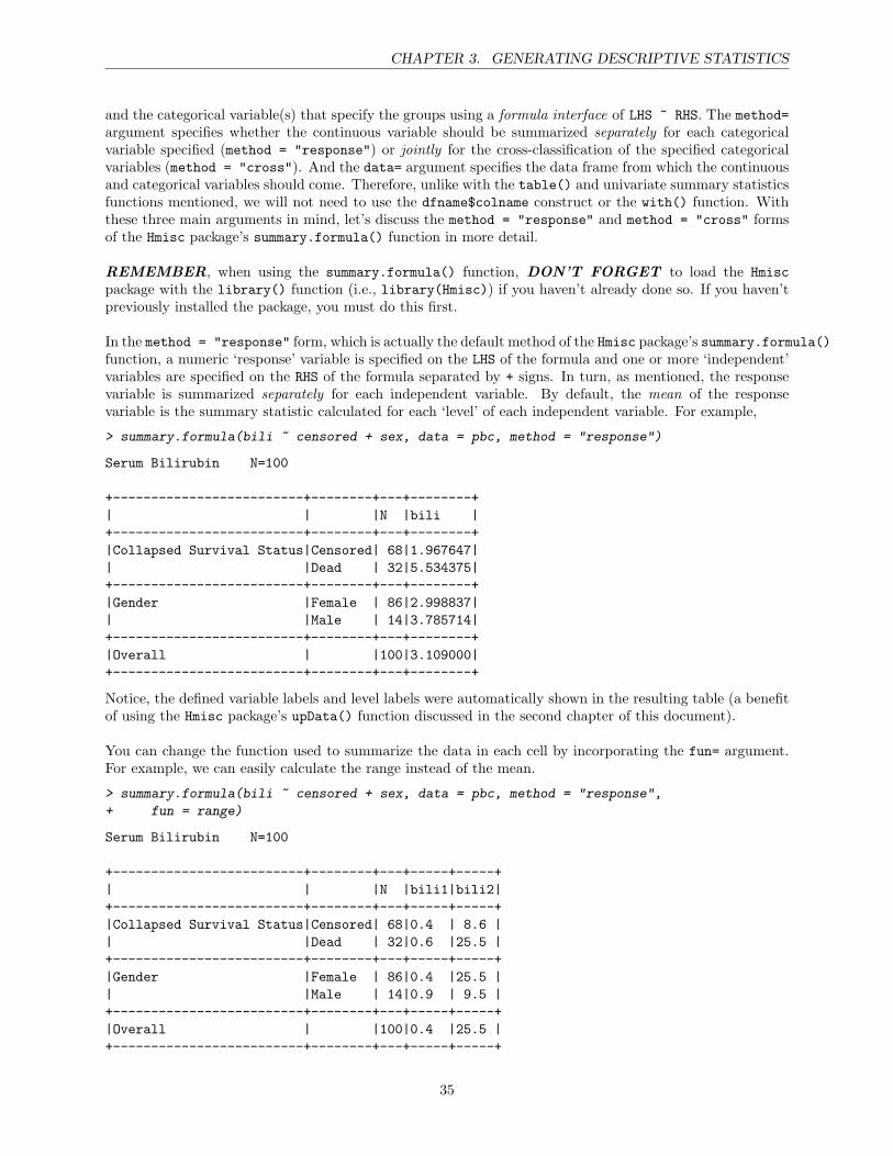
CHAPTER 3. GENERATING DESCRIPTIVE STATISTICS
and the categorical variable(s) that specify the groups using a formula interface of LHS ~ RHS. The method=argument specifies whether the continuous variable should be summarized separately for each categoricalvariable specified (method = "response") or jointly for the cross-classification of the specified categoricalvariables (method = "cross"). And the data= argument specifies the data frame from which the continuousand categorical variables should come. Therefore, unlike with the table() and univariate summary statisticsfunctions mentioned, we will not need to use the dfname$colname construct or the with() function. Withthese three main arguments in mind, let’s discuss the method = "response" and method = "cross" formsof the Hmisc package’s summary.formula() function in more detail.
REMEMBER, when using the summary.formula() function, DON’T FORGET to load the Hmiscpackage with the library() function (i.e., library(Hmisc)) if you haven’t already done so. If you haven’tpreviously installed the package, you must do this first.
In the method = "response" form, which is actually the default method of the Hmisc package’s summary.formula()function, a numeric ‘response’ variable is specified on the LHS of the formula and one or more ‘independent’variables are specified on the RHS of the formula separated by + signs. In turn, as mentioned, the responsevariable is summarized separately for each independent variable. By default, the mean of the responsevariable is the summary statistic calculated for each ‘level’ of each independent variable. For example,
> summary.formula(bili ~ censored + sex, data = pbc, method = "response")
Serum Bilirubin N=100
+-------------------------+--------+---+--------+| | |N |bili |+-------------------------+--------+---+--------+|Collapsed Survival Status|Censored| 68|1.967647|| |Dead | 32|5.534375|+-------------------------+--------+---+--------+|Gender |Female | 86|2.998837|| |Male | 14|3.785714|+-------------------------+--------+---+--------+|Overall | |100|3.109000|+-------------------------+--------+---+--------+
Notice, the defined variable labels and level labels were automatically shown in the resulting table (a benefitof using the Hmisc package’s upData() function discussed in the second chapter of this document).
You can change the function used to summarize the data in each cell by incorporating the fun= argument.For example, we can easily calculate the range instead of the mean.
> summary.formula(bili ~ censored + sex, data = pbc, method = "response",
+ fun = range)
Serum Bilirubin N=100
+-------------------------+--------+---+-----+-----+| | |N |bili1|bili2|+-------------------------+--------+---+-----+-----+|Collapsed Survival Status|Censored| 68|0.4 | 8.6 || |Dead | 32|0.6 |25.5 |+-------------------------+--------+---+-----+-----+|Gender |Female | 86|0.4 |25.5 || |Male | 14|0.9 | 9.5 |+-------------------------+--------+---+-----+-----+|Overall | |100|0.4 |25.5 |+-------------------------+--------+---+-----+-----+
35

CHAPTER 3. GENERATING DESCRIPTIVE STATISTICS
The function you specify with the fun= argument can even be self-defined. For example,
> summary.formula(bili ~ censored + sex, data = pbc, method = "response",
+ fun = function(x) {
+ c(Median = median(x), Min = min(x), Max = max(x))
+ })
Serum Bilirubin N=100
+-------------------------+--------+---+------+---+----+| | |N |Median|Min|Max |+-------------------------+--------+---+------+---+----+|Collapsed Survival Status|Censored| 68|1.05 |0.4| 8.6|| |Dead | 32|3.55 |0.6|25.5|+-------------------------+--------+---+------+---+----+|Gender |Female | 86|1.35 |0.4|25.5|| |Male | 14|2.70 |0.9| 9.5|+-------------------------+--------+---+------+---+----+|Overall | |100|1.60 |0.4|25.5|+-------------------------+--------+---+------+---+----+
You’ll notice that a final row labeled Overall is automatically (by default) calculated and printed, whichspecifies the global summary of the response variable. You can suppress this calculation and printing by spec-ifying overall = FALSE in your summary.formula() function invocation. In addition, unlike the univariatesummary statistics functions mentioned, the Hmisc package’s summary.formula() function by default alsoremoves any missing values from the response variable before calculating any summary statistics – na.rm =TRUE. For example,
> summary.formula(chol ~ drug + ascites, data = pbc, method = "response",
+ fun = median)
Serum Cholesterol N=68, 32 Missing
+-------------------+---------------+--+-----+| | |N |chol |+-------------------+---------------+--+-----+|Treatment |D-penicillamine|36|335.0|| |Placebo |32|324.5|+-------------------+---------------+--+-----+|Presence of Ascites|No |64|329.5|| |Yes | 4|288.5|+-------------------+---------------+--+-----+|Overall | |68|329.5|+-------------------+---------------+--+-----+
If an independent variable(s) specified on the RHS of the formula contain(s) more missing values than theresponse variable then missing values are counted as their own category when subsetting the response variableby the ‘levels’ of each categorical variable – na.include = TRUE. For example,
> summary.formula(fuyrs ~ drug + ascites, data = pbc, method = "response",
+ fun = median)
Follow Up N=100
+-------------------+---------------+---+--------+| | |N |fuyrs |
36
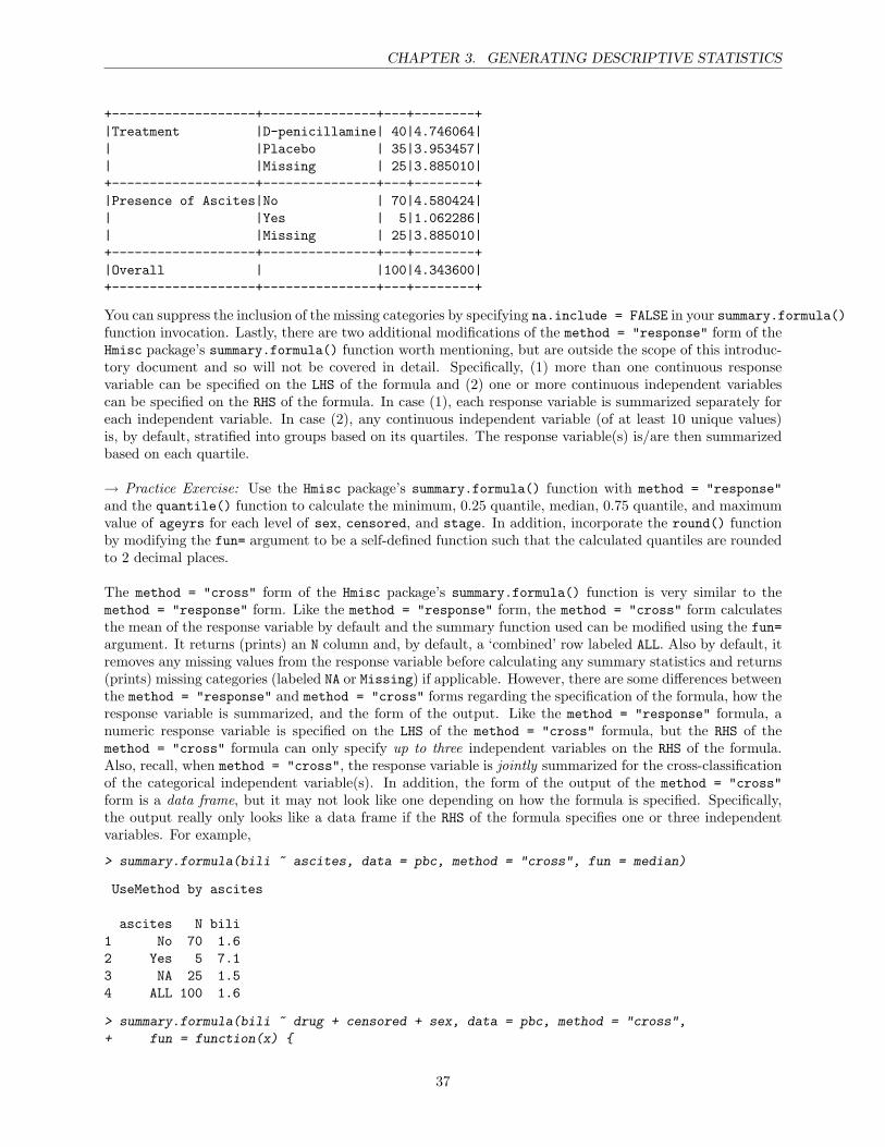
CHAPTER 3. GENERATING DESCRIPTIVE STATISTICS
+-------------------+---------------+---+--------+|Treatment |D-penicillamine| 40|4.746064|| |Placebo | 35|3.953457|| |Missing | 25|3.885010|+-------------------+---------------+---+--------+|Presence of Ascites|No | 70|4.580424|| |Yes | 5|1.062286|| |Missing | 25|3.885010|+-------------------+---------------+---+--------+|Overall | |100|4.343600|+-------------------+---------------+---+--------+
You can suppress the inclusion of the missing categories by specifying na.include = FALSE in your summary.formula()function invocation. Lastly, there are two additional modifications of the method = "response" form of theHmisc package’s summary.formula() function worth mentioning, but are outside the scope of this introduc-tory document and so will not be covered in detail. Specifically, (1) more than one continuous responsevariable can be specified on the LHS of the formula and (2) one or more continuous independent variablescan be specified on the RHS of the formula. In case (1), each response variable is summarized separately foreach independent variable. In case (2), any continuous independent variable (of at least 10 unique values)is, by default, stratified into groups based on its quartiles. The response variable(s) is/are then summarizedbased on each quartile.
→ Practice Exercise: Use the Hmisc package’s summary.formula() function with method = "response"and the quantile() function to calculate the minimum, 0.25 quantile, median, 0.75 quantile, and maximumvalue of ageyrs for each level of sex, censored, and stage. In addition, incorporate the round() functionby modifying the fun= argument to be a self-defined function such that the calculated quantiles are roundedto 2 decimal places.
The method = "cross" form of the Hmisc package’s summary.formula() function is very similar to themethod = "response" form. Like the method = "response" form, the method = "cross" form calculatesthe mean of the response variable by default and the summary function used can be modified using the fun=argument. It returns (prints) an N column and, by default, a ‘combined’ row labeled ALL. Also by default, itremoves any missing values from the response variable before calculating any summary statistics and returns(prints) missing categories (labeled NA or Missing) if applicable. However, there are some differences betweenthe method = "response" and method = "cross" forms regarding the specification of the formula, how theresponse variable is summarized, and the form of the output. Like the method = "response" formula, anumeric response variable is specified on the LHS of the method = "cross" formula, but the RHS of themethod = "cross" formula can only specify up to three independent variables on the RHS of the formula.Also, recall, when method = "cross", the response variable is jointly summarized for the cross-classificationof the categorical independent variable(s). In addition, the form of the output of the method = "cross"form is a data frame, but it may not look like one depending on how the formula is specified. Specifically,the output really only looks like a data frame if the RHS of the formula specifies one or three independentvariables. For example,
> summary.formula(bili ~ ascites, data = pbc, method = "cross", fun = median)
UseMethod by ascites
ascites N bili1 No 70 1.62 Yes 5 7.13 NA 25 1.54 ALL 100 1.6
> summary.formula(bili ~ drug + censored + sex, data = pbc, method = "cross",
+ fun = function(x) {
37

CHAPTER 3. GENERATING DESCRIPTIVE STATISTICS
+ c(Mean = mean(x), SD = sd(x), Median = median(x), Min = min(x),
+ Max = max(x))
+ })
function by drug, censored, sex list(x = ) by drug, censored, sex { by drug, censored, sex NULL by drug, censored, sex
drug censored sex N Mean SD.bili Median Min Max1 D-penicillamine Censored Female 21 1.304762 1.173233 0.90 0.4 5.52 Placebo Censored Female 19 1.784211 1.682677 1.00 0.4 6.43 NA Censored Female 19 2.021053 2.278542 1.00 0.6 8.14 ALL Censored Female 59 1.689831 1.748467 1.00 0.4 8.15 D-penicillamine Dead Female 13 3.238462 2.087478 3.20 0.6 7.16 Placebo Dead Female 11 8.254545 8.798791 5.10 0.8 25.57 NA Dead Female 3 8.433333 6.995951 7.10 2.2 16.08 ALL Dead Female 27 5.859259 6.494510 3.60 0.6 25.59 D-penicillamine ALL Female 34 2.044118 1.824445 1.15 0.4 7.110 Placebo ALL Female 30 4.156667 6.205708 2.10 0.4 25.511 NA ALL Female 22 2.895455 3.766200 1.35 0.6 16.012 ALL ALL Female 86 2.998837 4.333142 1.35 0.4 25.513 D-penicillamine Censored Male 3 4.333333 2.458319 3.50 2.4 7.114 Placebo Censored Male 4 4.250000 3.535062 3.75 0.9 8.615 NA Censored Male 2 2.050000 1.343503 2.05 1.1 3.016 ALL Censored Male 9 3.788889 2.719579 3.00 0.9 8.617 D-penicillamine Dead Male 3 2.633333 1.234234 2.30 1.6 4.018 Placebo Dead Male 1 1.500000 NA 1.50 1.5 1.519 NA Dead Male 1 9.500000 NA 9.50 9.5 9.520 ALL Dead Male 5 3.780000 3.350672 2.30 1.5 9.521 D-penicillamine ALL Male 6 3.483333 1.973238 2.95 1.6 7.122 Placebo ALL Male 5 3.700000 3.299242 1.90 0.9 8.623 NA ALL Male 3 4.533333 4.404921 3.00 1.1 9.524 ALL ALL Male 14 3.785714 2.829476 2.70 0.9 9.525 D-penicillamine Censored ALL 24 1.683333 1.664114 1.05 0.4 7.126 Placebo Censored ALL 23 2.213043 2.221241 1.00 0.4 8.627 NA Censored ALL 21 2.023810 2.182408 1.10 0.6 8.128 ALL Censored ALL 68 1.967647 2.010750 1.05 0.4 8.629 D-penicillamine Dead ALL 16 3.125000 1.936147 3.20 0.6 7.130 Placebo Dead ALL 12 7.691667 8.612935 4.35 0.8 25.531 NA Dead ALL 4 8.700000 5.737014 8.30 2.2 16.032 ALL Dead ALL 32 5.534375 6.116588 3.55 0.6 25.533 D-penicillamine ALL ALL 40 2.260000 1.893823 1.60 0.4 7.134 Placebo ALL ALL 35 4.091429 5.844171 2.10 0.4 25.535 NA ALL ALL 25 3.092000 3.784609 1.50 0.6 16.036 ALL ALL ALL 100 3.109000 4.153010 1.60 0.4 25.5
However, if the RHS of the formula specifies two independent variables then the output is printed in a tableformat, where the levels of the first independent variable denote the rows, the levels of the second independentvariable denote the columns, and the values in each cell represent the summary of the response variable. Forexample,
> summary.formula(bili ~ censored + sex, data = pbc, method = "cross",
+ fun = function(x) {
+ c(Mean = mean(x), SD = sd(x), Median = median(x), Min = min(x),
+ Max = max(x))
+ })
38
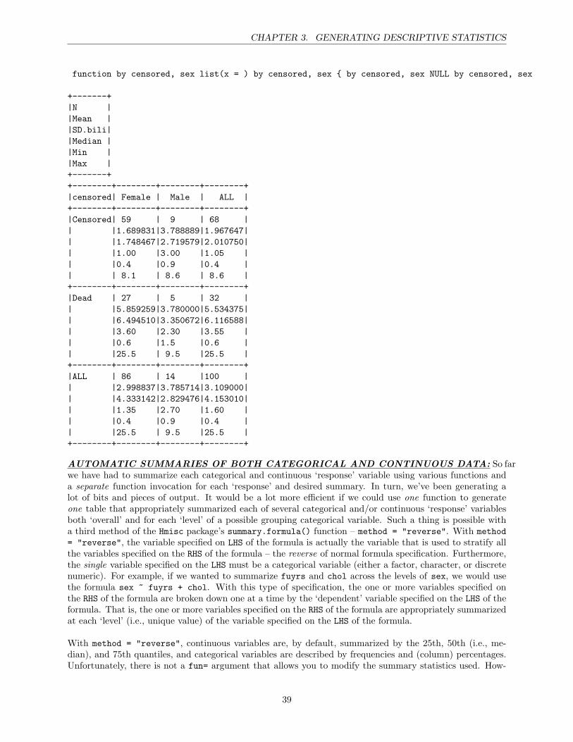
CHAPTER 3. GENERATING DESCRIPTIVE STATISTICS
function by censored, sex list(x = ) by censored, sex { by censored, sex NULL by censored, sex
+-------+|N ||Mean ||SD.bili||Median ||Min ||Max |+-------++--------+--------+--------+--------+|censored| Female | Male | ALL |+--------+--------+--------+--------+|Censored| 59 | 9 | 68 || |1.689831|3.788889|1.967647|| |1.748467|2.719579|2.010750|| |1.00 |3.00 |1.05 || |0.4 |0.9 |0.4 || | 8.1 | 8.6 | 8.6 |+--------+--------+--------+--------+|Dead | 27 | 5 | 32 || |5.859259|3.780000|5.534375|| |6.494510|3.350672|6.116588|| |3.60 |2.30 |3.55 || |0.6 |1.5 |0.6 || |25.5 | 9.5 |25.5 |+--------+--------+--------+--------+|ALL | 86 | 14 |100 || |2.998837|3.785714|3.109000|| |4.333142|2.829476|4.153010|| |1.35 |2.70 |1.60 || |0.4 |0.9 |0.4 || |25.5 | 9.5 |25.5 |+--------+--------+--------+--------+
AUTOMATIC SUMMARIES OF BOTH CATEGORICAL AND CONTINUOUS DATA: So farwe have had to summarize each categorical and continuous ‘response’ variable using various functions anda separate function invocation for each ‘response’ and desired summary. In turn, we’ve been generating alot of bits and pieces of output. It would be a lot more efficient if we could use one function to generateone table that appropriately summarized each of several categorical and/or continuous ‘response’ variablesboth ‘overall’ and for each ‘level’ of a possible grouping categorical variable. Such a thing is possible witha third method of the Hmisc package’s summary.formula() function – method = "reverse". With method= "reverse", the variable specified on LHS of the formula is actually the variable that is used to stratify allthe variables specified on the RHS of the formula – the reverse of normal formula specification. Furthermore,the single variable specified on the LHS must be a categorical variable (either a factor, character, or discretenumeric). For example, if we wanted to summarize fuyrs and chol across the levels of sex, we would usethe formula sex ~ fuyrs + chol. With this type of specification, the one or more variables specified onthe RHS of the formula are broken down one at a time by the ‘dependent’ variable specified on the LHS of theformula. That is, the one or more variables specified on the RHS of the formula are appropriately summarizedat each ‘level’ (i.e., unique value) of the variable specified on the LHS of the formula.
With method = "reverse", continuous variables are, by default, summarized by the 25th, 50th (i.e., me-dian), and 75th quantiles, and categorical variables are described by frequencies and (column) percentages.Unfortunately, there is not a fun= argument that allows you to modify the summary statistics used. How-
39
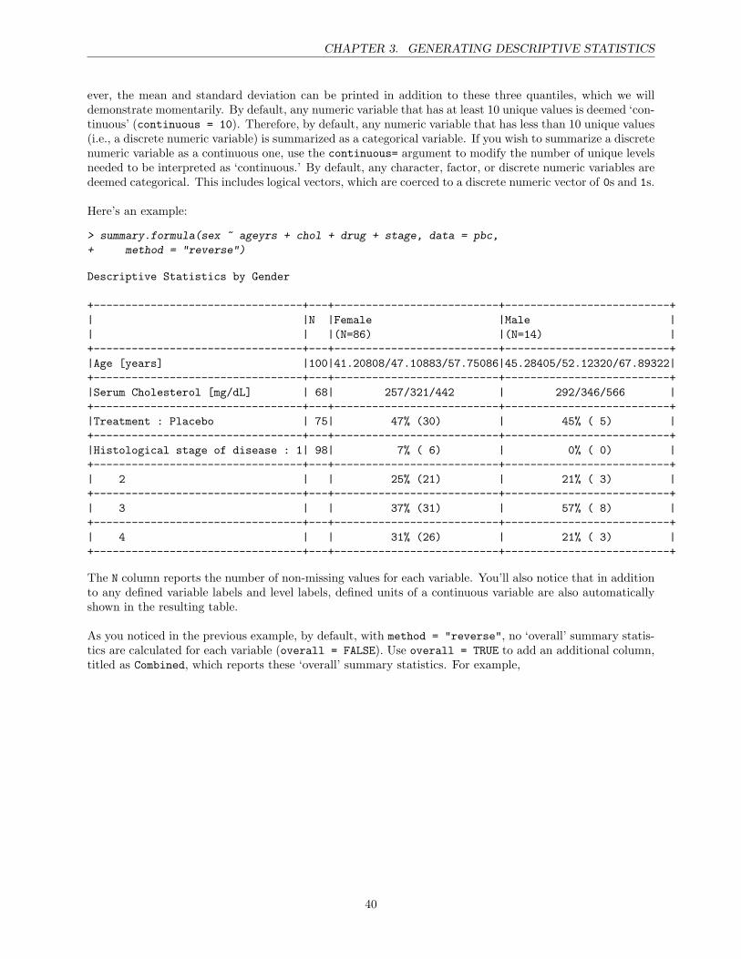
CHAPTER 3. GENERATING DESCRIPTIVE STATISTICS
ever, the mean and standard deviation can be printed in addition to these three quantiles, which we willdemonstrate momentarily. By default, any numeric variable that has at least 10 unique values is deemed ‘con-tinuous’ (continuous = 10). Therefore, by default, any numeric variable that has less than 10 unique values(i.e., a discrete numeric variable) is summarized as a categorical variable. If you wish to summarize a discretenumeric variable as a continuous one, use the continuous= argument to modify the number of unique levelsneeded to be interpreted as ‘continuous.’ By default, any character, factor, or discrete numeric variables aredeemed categorical. This includes logical vectors, which are coerced to a discrete numeric vector of 0s and 1s.
Here’s an example:
> summary.formula(sex ~ ageyrs + chol + drug + stage, data = pbc,
+ method = "reverse")
Descriptive Statistics by Gender
+---------------------------------+---+--------------------------+--------------------------+| |N |Female |Male || | |(N=86) |(N=14) |+---------------------------------+---+--------------------------+--------------------------+|Age [years] |100|41.20808/47.10883/57.75086|45.28405/52.12320/67.89322|+---------------------------------+---+--------------------------+--------------------------+|Serum Cholesterol [mg/dL] | 68| 257/321/442 | 292/346/566 |+---------------------------------+---+--------------------------+--------------------------+|Treatment : Placebo | 75| 47% (30) | 45% ( 5) |+---------------------------------+---+--------------------------+--------------------------+|Histological stage of disease : 1| 98| 7% ( 6) | 0% ( 0) |+---------------------------------+---+--------------------------+--------------------------+| 2 | | 25% (21) | 21% ( 3) |+---------------------------------+---+--------------------------+--------------------------+| 3 | | 37% (31) | 57% ( 8) |+---------------------------------+---+--------------------------+--------------------------+| 4 | | 31% (26) | 21% ( 3) |+---------------------------------+---+--------------------------+--------------------------+
The N column reports the number of non-missing values for each variable. You’ll also notice that in additionto any defined variable labels and level labels, defined units of a continuous variable are also automaticallyshown in the resulting table.
As you noticed in the previous example, by default, with method = "reverse", no ‘overall’ summary statis-tics are calculated for each variable (overall = FALSE). Use overall = TRUE to add an additional column,titled as Combined, which reports these ‘overall’ summary statistics. For example,
40
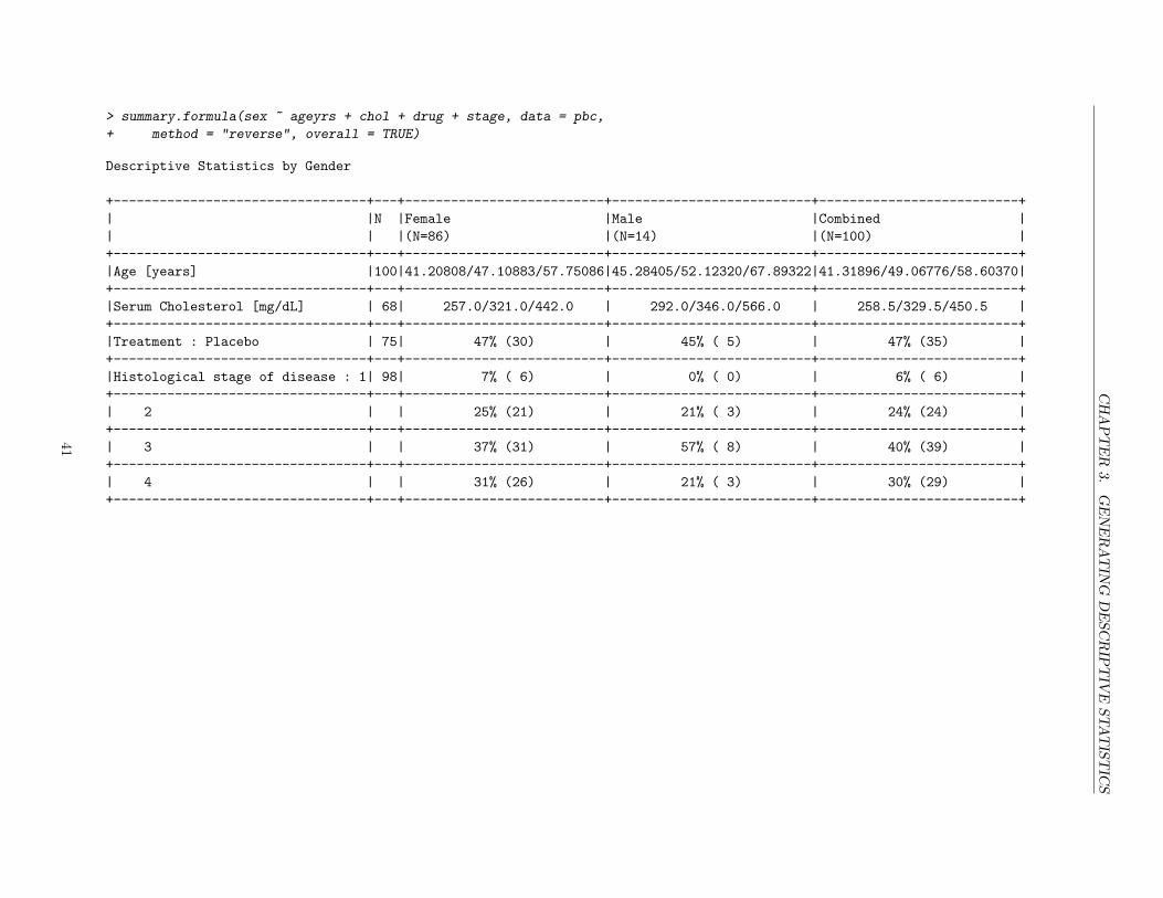
CH
AP
TE
R3.
GE
NE
RA
TIN
GD
ESC
RIP
TIV
ESTA
TIS
TIC
S
> summary.formula(sex ~ ageyrs + chol + drug + stage, data = pbc,
+ method = "reverse", overall = TRUE)
Descriptive Statistics by Gender
+---------------------------------+---+--------------------------+--------------------------+--------------------------+| |N |Female |Male |Combined || | |(N=86) |(N=14) |(N=100) |+---------------------------------+---+--------------------------+--------------------------+--------------------------+|Age [years] |100|41.20808/47.10883/57.75086|45.28405/52.12320/67.89322|41.31896/49.06776/58.60370|+---------------------------------+---+--------------------------+--------------------------+--------------------------+|Serum Cholesterol [mg/dL] | 68| 257.0/321.0/442.0 | 292.0/346.0/566.0 | 258.5/329.5/450.5 |+---------------------------------+---+--------------------------+--------------------------+--------------------------+|Treatment : Placebo | 75| 47% (30) | 45% ( 5) | 47% (35) |+---------------------------------+---+--------------------------+--------------------------+--------------------------+|Histological stage of disease : 1| 98| 7% ( 6) | 0% ( 0) | 6% ( 6) |+---------------------------------+---+--------------------------+--------------------------+--------------------------+| 2 | | 25% (21) | 21% ( 3) | 24% (24) |+---------------------------------+---+--------------------------+--------------------------+--------------------------+| 3 | | 37% (31) | 57% ( 8) | 40% (39) |+---------------------------------+---+--------------------------+--------------------------+--------------------------+| 4 | | 31% (26) | 21% ( 3) | 30% (29) |+---------------------------------+---+--------------------------+--------------------------+--------------------------+
41
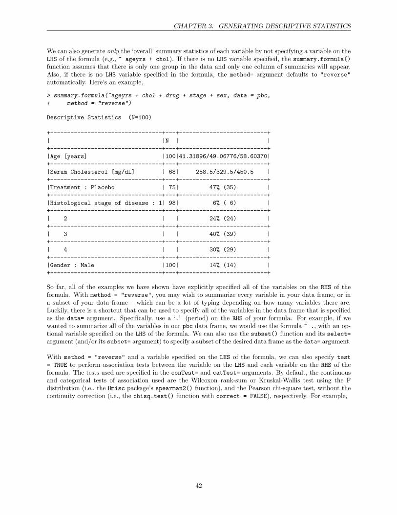
CHAPTER 3. GENERATING DESCRIPTIVE STATISTICS
We can also generate only the ‘overall’ summary statistics of each variable by not specifying a variable on theLHS of the formula (e.g., ~ ageyrs + chol). If there is no LHS variable specified, the summary.formula()function assumes that there is only one group in the data and only one column of summaries will appear.Also, if there is no LHS variable specified in the formula, the method= argument defaults to "reverse"automatically. Here’s an example,
> summary.formula(~ageyrs + chol + drug + stage + sex, data = pbc,
+ method = "reverse")
Descriptive Statistics (N=100)
+---------------------------------+---+--------------------------+| |N | |+---------------------------------+---+--------------------------+|Age [years] |100|41.31896/49.06776/58.60370|+---------------------------------+---+--------------------------+|Serum Cholesterol [mg/dL] | 68| 258.5/329.5/450.5 |+---------------------------------+---+--------------------------+|Treatment : Placebo | 75| 47% (35) |+---------------------------------+---+--------------------------+|Histological stage of disease : 1| 98| 6% ( 6) |+---------------------------------+---+--------------------------+| 2 | | 24% (24) |+---------------------------------+---+--------------------------+| 3 | | 40% (39) |+---------------------------------+---+--------------------------+| 4 | | 30% (29) |+---------------------------------+---+--------------------------+|Gender : Male |100| 14% (14) |+---------------------------------+---+--------------------------+
So far, all of the examples we have shown have explicitly specified all of the variables on the RHS of theformula. With method = "reverse", you may wish to summarize every variable in your data frame, or ina subset of your data frame – which can be a lot of typing depending on how many variables there are.Luckily, there is a shortcut that can be used to specify all of the variables in the data frame that is specifiedas the data= argument. Specifically, use a ‘.’ (period) on the RHS of your formula. For example, if wewanted to summarize all of the variables in our pbc data frame, we would use the formula ~ ., with an op-tional variable specified on the LHS of the formula. We can also use the subset() function and its select=argument (and/or its subset= argument) to specify a subset of the desired data frame as the data= argument.
With method = "reverse" and a variable specified on the LHS of the formula, we can also specify test= TRUE to perform association tests between the variable on the LHS and each variable on the RHS of theformula. The tests used are specified in the conTest= and catTest= arguments. By default, the continuousand categorical tests of association used are the Wilcoxon rank-sum or Kruskal-Wallis test using the Fdistribution (i.e., the Hmisc package’s spearman2() function), and the Pearson chi-square test, without thecontinuity correction (i.e., the chisq.test() function with correct = FALSE), respectively. For example,
42
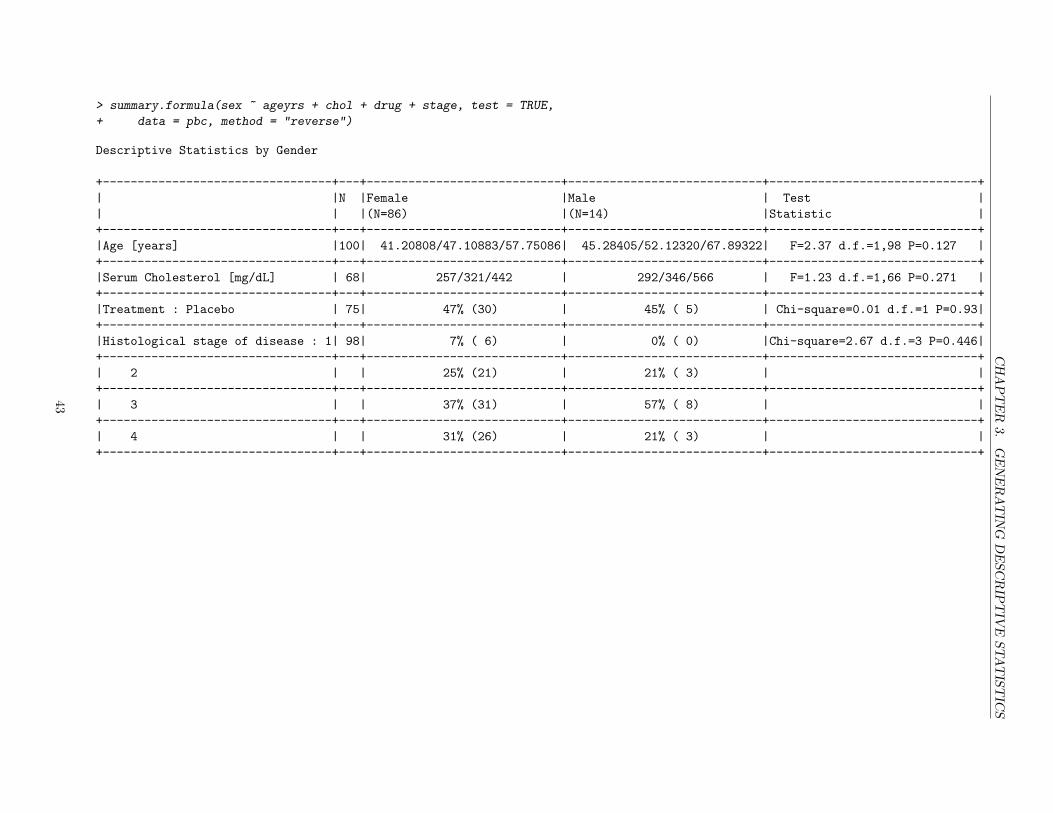
CH
AP
TE
R3.
GE
NE
RA
TIN
GD
ESC
RIP
TIV
ESTA
TIS
TIC
S
> summary.formula(sex ~ ageyrs + chol + drug + stage, test = TRUE,
+ data = pbc, method = "reverse")
Descriptive Statistics by Gender
+---------------------------------+---+----------------------------+----------------------------+------------------------------+| |N |Female |Male | Test || | |(N=86) |(N=14) |Statistic |+---------------------------------+---+----------------------------+----------------------------+------------------------------+|Age [years] |100| 41.20808/47.10883/57.75086| 45.28405/52.12320/67.89322| F=2.37 d.f.=1,98 P=0.127 |+---------------------------------+---+----------------------------+----------------------------+------------------------------+|Serum Cholesterol [mg/dL] | 68| 257/321/442 | 292/346/566 | F=1.23 d.f.=1,66 P=0.271 |+---------------------------------+---+----------------------------+----------------------------+------------------------------+|Treatment : Placebo | 75| 47% (30) | 45% ( 5) | Chi-square=0.01 d.f.=1 P=0.93|+---------------------------------+---+----------------------------+----------------------------+------------------------------+|Histological stage of disease : 1| 98| 7% ( 6) | 0% ( 0) |Chi-square=2.67 d.f.=3 P=0.446|+---------------------------------+---+----------------------------+----------------------------+------------------------------+| 2 | | 25% (21) | 21% ( 3) | |+---------------------------------+---+----------------------------+----------------------------+------------------------------+| 3 | | 37% (31) | 57% ( 8) | |+---------------------------------+---+----------------------------+----------------------------+------------------------------+| 4 | | 31% (26) | 21% ( 3) | |+---------------------------------+---+----------------------------+----------------------------+------------------------------+
43
CHAPTER 3. GENERATING DESCRIPTIVE STATISTICS
You can also optionally specify overall = TRUE with test = TRUE. In this case, the tests are correctlyperformed (i.e., they ignore the values in the Combined column).
As you probably noticed, the way the output of the Hmisc package’s summary.formula() function withmethod = "reverse" is printed by default is not that desirable. For instance, there are varying numbers ofdecimal places and not all levels of all categorical variables are shown. Luckily there is a print method that cor-responds to the summary.formula() function with method = "reverse" output – print.summary.formula.reverse().We can specify our method = "reverse" form of our summary.formula() function invocation as the data ar-gument to a print.summary.formula.reverse() method invocation and use the print.summary.formula.reverse()arguments to print the output as desired.
Specifically, use the digits= argument to specify the number of significant digits to print. By default, thecurrent value of the digits system option (i.e., options("digits")) is used, which is 7.
By default, the number of non-missing observations for each RHS variable (i.e., the N column) is printed onlyif any of the counts of non-missing values of the RHS variables differs from the total number of non-missingvalues of the LHS variable. Specify prn = TRUE to always print the number of non-missing observations foreach RHS variable.
You can modify the way the frequencies and column percentages for categorical variables are printed usingthe npct= and pctdig= arguments. In general, the npct= argument specifies which counts are to be printed tothe right of percentages. By default, only the numerator of the percentage is printed (npct = "numerator").Use npct = "both" to print both numerator and denominator, which is very useful when your data (boththe LHS and RHS variables) contain missing values. You can also specify npct = "denominator" or npct ="none". The pctdig= argument specifies the number of digits to the right of the decimal place for printingpercentages. By default, pctdig = 0, so percents will be rounded to the nearest percent.
By default, for method="reverse", summary.formula() function objects will be printed by removing ‘redun-dant’ entries from percentage tables for binary categorical variables – exclude1 = TRUE. This means thatonly one of the two levels for any binary categorical variable will be printed. For example, only the Placebolevel of drug was summarized in our printed output. The idea is that, for a binary categorical variable, ifyou know the frequency of one level and the denominator then you can easily calculate the frequency of theother level. To override this, use exclude1 = FALSE.
Going one step further, you probably noticed that the summary of the first level of any categorical variable(binary or more levels) was printed on the same line as the variable label – long = FALSE. To print theresult for the first level on a new line, use long = TRUE.
When you use test = TRUE, you can optionally specify the pdig=, eps=, and prtest= arguments to controlthe number of digits to the right of the decimal place for printing p-values, the p-value ‘cutoff’, and thetest statistic components that are printed, respectively. By default, pdig = 3, eps = 0.001, which meanany p-values less than 0.001 will be printed as < 0.001, and prtest = c("P", "stat", "df", "name"),which means the name of the test statistic (F or Chi-square), the value of the test statistic, the degree(s)of freedom, and the p-value are all printed. An alternative is to use prtest = "P", which prints only thep-values.
Lastly, specify prmsd = TRUE to print the mean and standard deviation of a continuous variable in additionto the three quantiles. Keep in mind though, that this will make the individual columns even wider.
As an example, let’s incorporate some of these printing arguments,
> print(summary.formula(sex ~ ageyrs + chol + drug + stage, overall = TRUE,
+ method = "reverse", data = pbc), digits = 3, npct = "both",
+ pctdig = 2, exclude1 = FALSE, long = TRUE)
44
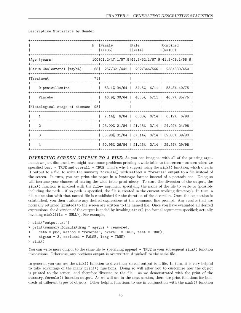
CHAPTER 3. GENERATING DESCRIPTIVE STATISTICS
Descriptive Statistics by Gender
+-----------------------------+---+--------------+--------------+--------------+| |N |Female |Male |Combined || | |(N=86) |(N=14) |(N=100) |+-----------------------------+---+--------------+--------------+--------------+|Age [years] |100|41.2/47.1/57.8|45.3/52.1/67.9|41.3/49.1/58.6|+-----------------------------+---+--------------+--------------+--------------+|Serum Cholesterol [mg/dL] | 68| 257/321/442 | 292/346/566 | 258/330/450 |+-----------------------------+---+--------------+--------------+--------------+|Treatment | 75| | | |+-----------------------------+---+--------------+--------------+--------------+| D-penicillamine | | 53.1% 34/64 | 54.5% 6/11 | 53.3% 40/75 |+-----------------------------+---+--------------+--------------+--------------+| Placebo | | 46.9% 30/64 | 45.5% 5/11 | 46.7% 35/75 |+-----------------------------+---+--------------+--------------+--------------+|Histological stage of disease| 98| | | |+-----------------------------+---+--------------+--------------+--------------+| 1 | | 7.14% 6/84 | 0.00% 0/14 | 6.12% 6/98 |+-----------------------------+---+--------------+--------------+--------------+| 2 | | 25.00% 21/84 | 21.43% 3/14 | 24.49% 24/98 |+-----------------------------+---+--------------+--------------+--------------+| 3 | | 36.90% 31/84 | 57.14% 8/14 | 39.80% 39/98 |+-----------------------------+---+--------------+--------------+--------------+| 4 | | 30.95% 26/84 | 21.43% 3/14 | 29.59% 29/98 |+-----------------------------+---+--------------+--------------+--------------+
DIVERTING SCREEN OUTPUT TO A FILE: As you can imagine, with all of the printing argu-ments we just discussed, we might have some problems printing a wide table to the screen – as seen when wespecified test = TRUE and overall = TRUE. That’s why I suggest using the sink() function, which divertsR output to a file, to write the summary.formula() with method = "reverse" output to a file instead ofthe screen. In turn, you can print the paper in a landscape format instead of a portrait one. Doing sowill increase your chances of having the wide table print nicely. To start the diversion of the output, thesink() function is invoked with the file= argument specifying the name of the file to write to (possiblyincluding the path – if no path is specified, the file is created in the current working directory). In turn, afile connection with that named file is established for the duration of the diversion. Once the connection isestablished, you then evaluate any desired expressions at the command line prompt. Any results that arenormally returned (printed) to the screen are written to the named file. Once you have evaluated all desiredexpressions, the diversion of the output is ended by invoking sink() (no formal arguments specified; actuallyinvoking sink(file = NULL)). For example,
> sink("output.txt")> print(summary.formula(drug ~ ageyrs + censored,+ data = pbc, method = "reverse", overall = TRUE, test = TRUE),+ digits = 3, exclude1 = FALSE, long = TRUE)> sink()
You can write more output to the same file by specifying append = TRUE in your subsequent sink() functioninvocations. Otherwise, any previous output is overwritten if ‘sinked’ to the same file.
In general, you can use the sink() function to divert any screen output to a file. In turn, it is very helpfulto take advantage of the many print() functions. Doing so will allow you to customize how the objectis printed to the screen, and therefore diverted to the file – as we demonstrated with the print of thesummary.formula() function output. As we will see in the next section, there are print functions for hun-dreds of different types of objects. Other helpful functions to use in conjunction with the sink() function
45
CHAPTER 3. GENERATING DESCRIPTIVE STATISTICS
are the cat() and paste() functions, which we discuss in the ‘Data Export’ section of the second document.
The major draw back to the sink() function is that it doesn’t write the invoked function expressions to thespecified file. Therefore the file contains only evaluated results, not the function expressions used to generatethose results. If you are interested in capturing this information too, I would recommend copying desiredoutput that has been returned (printed) to the screen and pasting it into your code file below the functionexpression that generated it. In turn, you can use the # symbol to comment out the copied output.
In the Windows version of R you also have two options under the File drop-menu: (1) Print. . . ; or (2) Saveto file. . . . These two options will print or save, respectively, the whole command line subwindow includingall submitted function expressions and all returned output and warning/error messages.
Lastly, another option for generating reproducible research with R and LATEX is Sweave – see the ‘Sweave,part I: Mixing R and LATEX’ article by Friedrich Leisch in the December 2002 issue of the R News newslet-ter, and http://www.ci.tuwien.ac.at/~leisch/Sweave/ for more information. Feel free to also check-outmy ‘Reproducible Research with R, LATEX, and Sweave’ lecture on my website.
→ Practice Exercise: Let’s summarize ageyrs, sex, bili, chol, album, ascites, drug, censored, and fuyrsacross the levels of stage. Let’s generate an ‘overall’ summary for each variable and test for any associationsbetween stage and any of the ‘response’ variables. Let’s direct the output to a file named "output.txt"and modify the printed output to include the mean and standard deviation of all continuous variables, to‘round’ to three significant digits, to show both the numerator and denominator of the frequencies, to printthe percentages to two decimal places, to show both levels of all binary categorical variables, to print the firstlevel of all categorical variable on a new line, and to print only the p-values (rounded to 4 decimal places)as the test output. Let’s then open the output.txt file with an appropriate text editor and see the result –you might have to turn off any word-wrapping to see the output nicely.
A THOUGHT TO END WITH: The action of many functions in R depend on the kind of object givenas the main argument. More specifically, these functions act with respect to the class (i.e., the definition)of the object specified as its main argument. These functions are called generic. In turn, for any genericfunction, there can be a number of different class specific methods where each method is a different functionthat corresponds to the action to be taken for a particular class of objects. For example, the summary()function is generic and generates a different summary for a vector, a data frame, or a formula:
> summary(pbc$ageyrs)
Min. 1st Qu. Median Mean 3rd Qu. Max.30.57 41.32 49.07 49.92 58.60 78.44
> summary(pbc)
id fudays statusMin. : 6.0 Min. : 216 Censored :621st Qu.:118.8 1st Qu.:1150 Censored due to liver treatment: 6Median :238.0 Median :1586 Dead :32Mean :223.2 Mean :18703rd Qu.:313.2 3rd Qu.:2546Max. :417.0 Max. :4453
drug age sex ascites biliD-penicillamine:40 Min. :11167 Female:86 No :70 Min. : 0.400Placebo :35 1st Qu.:15092 Male :14 Yes : 5 1st Qu.: 0.800NA's :25 Median :17922 NA's:25 Median : 1.600
Mean :18234 Mean : 3.1093rd Qu.:21405 3rd Qu.: 3.600
46
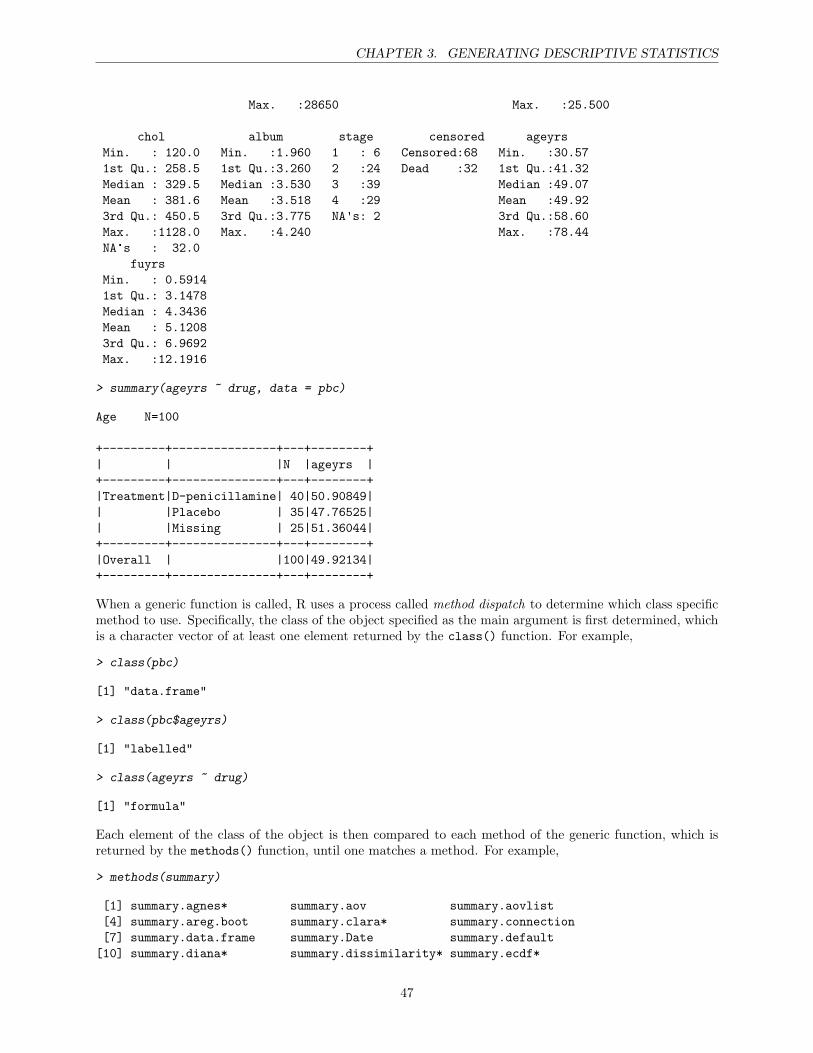
CHAPTER 3. GENERATING DESCRIPTIVE STATISTICS
Max. :28650 Max. :25.500
chol album stage censored ageyrsMin. : 120.0 Min. :1.960 1 : 6 Censored:68 Min. :30.571st Qu.: 258.5 1st Qu.:3.260 2 :24 Dead :32 1st Qu.:41.32Median : 329.5 Median :3.530 3 :39 Median :49.07Mean : 381.6 Mean :3.518 4 :29 Mean :49.923rd Qu.: 450.5 3rd Qu.:3.775 NA's: 2 3rd Qu.:58.60Max. :1128.0 Max. :4.240 Max. :78.44NA's : 32.0
fuyrsMin. : 0.59141st Qu.: 3.1478Median : 4.3436Mean : 5.12083rd Qu.: 6.9692Max. :12.1916
> summary(ageyrs ~ drug, data = pbc)
Age N=100
+---------+---------------+---+--------+| | |N |ageyrs |+---------+---------------+---+--------+|Treatment|D-penicillamine| 40|50.90849|| |Placebo | 35|47.76525|| |Missing | 25|51.36044|+---------+---------------+---+--------+|Overall | |100|49.92134|+---------+---------------+---+--------+
When a generic function is called, R uses a process called method dispatch to determine which class specificmethod to use. Specifically, the class of the object specified as the main argument is first determined, whichis a character vector of at least one element returned by the class() function. For example,
> class(pbc)
[1] "data.frame"
> class(pbc$ageyrs)
[1] "labelled"
> class(ageyrs ~ drug)
[1] "formula"
Each element of the class of the object is then compared to each method of the generic function, which isreturned by the methods() function, until one matches a method. For example,
> methods(summary)
[1] summary.agnes* summary.aov summary.aovlist[4] summary.areg.boot summary.clara* summary.connection[7] summary.data.frame summary.Date summary.default[10] summary.diana* summary.dissimilarity* summary.ecdf*
47
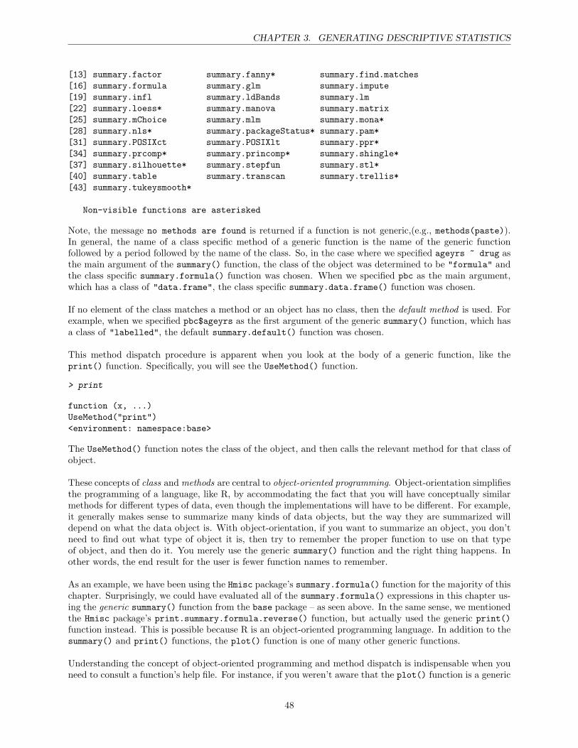
CHAPTER 3. GENERATING DESCRIPTIVE STATISTICS
[13] summary.factor summary.fanny* summary.find.matches[16] summary.formula summary.glm summary.impute[19] summary.infl summary.ldBands summary.lm[22] summary.loess* summary.manova summary.matrix[25] summary.mChoice summary.mlm summary.mona*[28] summary.nls* summary.packageStatus* summary.pam*[31] summary.POSIXct summary.POSIXlt summary.ppr*[34] summary.prcomp* summary.princomp* summary.shingle*[37] summary.silhouette* summary.stepfun summary.stl*[40] summary.table summary.transcan summary.trellis*[43] summary.tukeysmooth*
Non-visible functions are asterisked
Note, the message no methods are found is returned if a function is not generic,(e.g., methods(paste)).In general, the name of a class specific method of a generic function is the name of the generic functionfollowed by a period followed by the name of the class. So, in the case where we specified ageyrs ~ drug asthe main argument of the summary() function, the class of the object was determined to be "formula" andthe class specific summary.formula() function was chosen. When we specified pbc as the main argument,which has a class of "data.frame", the class specific summary.data.frame() function was chosen.
If no element of the class matches a method or an object has no class, then the default method is used. Forexample, when we specified pbc$ageyrs as the first argument of the generic summary() function, which hasa class of "labelled", the default summary.default() function was chosen.
This method dispatch procedure is apparent when you look at the body of a generic function, like theprint() function. Specifically, you will see the UseMethod() function.
function (x, ...)UseMethod("print")<environment: namespace:base>
The UseMethod() function notes the class of the object, and then calls the relevant method for that class ofobject.
These concepts of class and methods are central to object-oriented programming. Object-orientation simplifiesthe programming of a language, like R, by accommodating the fact that you will have conceptually similarmethods for different types of data, even though the implementations will have to be different. For example,it generally makes sense to summarize many kinds of data objects, but the way they are summarized willdepend on what the data object is. With object-orientation, if you want to summarize an object, you don’tneed to find out what type of object it is, then try to remember the proper function to use on that typeof object, and then do it. You merely use the generic summary() function and the right thing happens. Inother words, the end result for the user is fewer function names to remember.
As an example, we have been using the Hmisc package’s summary.formula() function for the majority of thischapter. Surprisingly, we could have evaluated all of the summary.formula() expressions in this chapter us-ing the generic summary() function from the base package – as seen above. In the same sense, we mentionedthe Hmisc package’s print.summary.formula.reverse() function, but actually used the generic print()function instead. This is possible because R is an object-oriented programming language. In addition to thesummary() and print() functions, the plot() function is one of many other generic functions.
Understanding the concept of object-oriented programming and method dispatch is indispensable when youneed to consult a function’s help file. For instance, if you weren’t aware that the plot() function is a generic
48
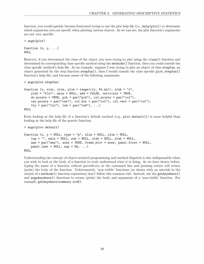
CHAPTER 3. GENERATING DESCRIPTIVE STATISTICS
function, you would quickly become frustrated trying to use the plot help file (i.e., help(plot)) to determinewhich arguments you can specify when plotting various objects. As we can see, the plot function’s argumentsare not very specific:
> args(plot)
function (x, y, ...)NULL
However, if you determined the class of the object you were trying to plot using the class() function anddetermined its corresponding class specific method using the methods() function, then you could consult theclass specific method’s help file. As an example, suppose I was trying to plot an object of class stepfun, anobject generated by the step function stepfun(), then I would consult the class specific plot.stepfun()function’s help file, and become aware of the following arguments:
> args(plot.stepfun)
function (x, xval, xlim, ylim = range(c(y, Fn.kn)), xlab = "x",ylab = "f(x)", main = NULL, add = FALSE, verticals = TRUE,do.points = TRUE, pch = par("pch"), col.points = par("col"),cex.points = par("cex"), col.hor = par("col"), col.vert = par("col"),lty = par("lty"), lwd = par("lwd"), ...)
NULL
Even looking at the help file of a function’s default method (e.g., plot.default()) is more helpful thanlooking at the help file of the generic function:
> args(plot.default)
function (x, y = NULL, type = "p", xlim = NULL, ylim = NULL,log = "", main = NULL, sub = NULL, xlab = NULL, ylab = NULL,ann = par("ann"), axes = TRUE, frame.plot = axes, panel.first = NULL,panel.last = NULL, asp = NA, ...)
NULL
Understanding the concept of object-oriented programming and method dispatch is also indispensable whenyou wish to look at the body of a function to truly understand what it is doing. As we have shown before,typing the name of a function without parentheses at the command line and pressing return will return(print) the body of the function. Unfortunately, ‘non-visible’ functions (as shown with an asterisk in theoutput of a methods() function expression) don’t follow this common rule. Instead, use the getAnywhere()and argsAnywhere() functions to return (print) the body and arguments of a ‘non-visible’ function. Forexample, getAnywhere(summary.ecdf).
49
Chapter 4
R Graphics
Learning objectiveTo understand how to incorporate high-level and low-level plotting functions and graphical parameters togenerate a customized graph.
TRADITIONAL GRAPHICS: R provides the usual range of standard statistical plots, including scat-terplots, boxplots, histograms, barplots, and basic 3D plots. Figure 4.1 on page 51 shows some examples fromPaul Murrell’s R Graphics book (Chapman & Hall/CRC, 2006). In R, these basic plots can be produced bya single function call, but plots can also be considered merely as starting points for producing more compleximages. For example, in the first four cases in Figure 4.1 on page 51, the basic plot type has been augmentedby adding additional labels, lines, and axes. This ability to add several graphical elements together to createthe final result is a fundamental feature of R graphics. And, as demonstrated in the last case in Figure 4.1on page 51, this ability also allows you to create a new plot ‘from scratch’ when no existing plot provides asensible starting point for creating the final plot that you desire.
TRELLIS GRAPHICS: In addition to these traditional statistical plots, R also provides an implementa-tion of trellis plots via the lattice package. Trellis plots embody a number of design principles proposed byBill Cleveland in his The Elements of Graphing Data and Visualizing Data books that are ‘aimed at ensuringaccurate and faithful communication of information via statistical plots.’ These principles are evident in anumber of new plot types and in the default choice of colors, symbol shapes, and line styles provided bytrellis plots. Furthermore, trellis plots provide a feature known as ‘multi-panel conditioning,’ which createsmultiple plots by splitting the data being plotted according to the levels of other variables. Figure 4.2 onpage 52 shows an example of a multi-panel trellis plot. The data are yields of several different varieties ofbarley at six sites, over two years. The plot consists of six ‘panels,’ one for each site. Each panel consists ofa dotplot showing yield for each site with different symbols used to distinguish different years, and a ‘strip’showing the name of the site.
In this document and the second document, we will only cover the traditional graphics system, which mainlyconsists of functions in the graphics and grDevices packages. If you are interested in learning more abouttrellis plots and the lattice package, I would highly recommend the book R Graphics by Paul Murrell(Chapman & Hall/CRC, 2006). We will also discuss some of the functions in the Hmisc package, as we havedone in previous section. Unlike the Hmisc package, the graphics package is automatically installed with Rand is loaded in every R session. REMEMBER, when using the functions in the Hmisc package, DON’TFORGET to load the Hmisc package with thelibrary() function (i.e., library(Hmisc)) if you haven’talready done so. If you haven’t previously installed the package, you must do this first.
BUILDING PLOTS IN LAYERS: Traditional R graphics follow a ‘painters model,’ which means thatgraphical output occurs in steps, with later output (possibly) obscuring any previous output that it overlaps.More specifically, in R, a traditional graphics plot is created by first calling a high-level plotting function
50
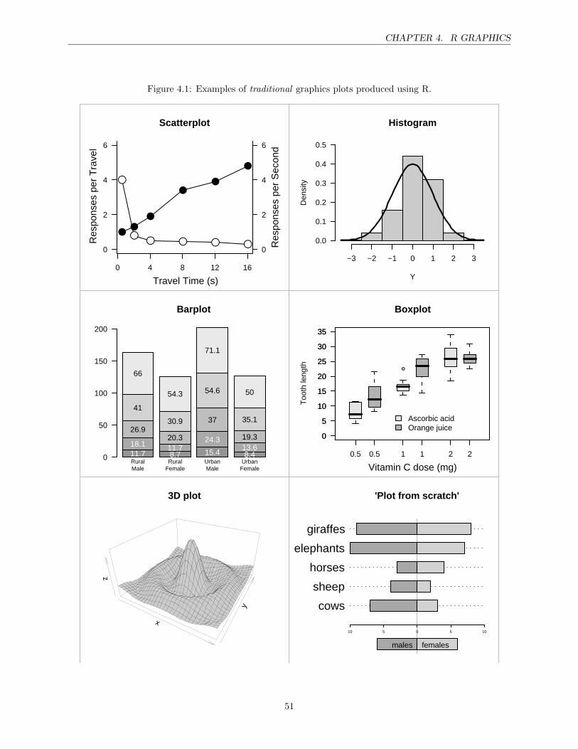
CHAPTER 4. R GRAPHICS
Figure 4.1: Examples of traditional graphics plots produced using R.
Scatterplot
●●
●
●●
●
●
●● ● ● ●
0 4 8 12 16
0
2
4
6
0
2
4
6
Travel Time (s)
Res
pons
es p
er T
rave
l
Res
pons
es p
er S
econ
d
Histogram
Y
Den
sity
−3 −2 −1 0 1 2 3
0.0
0.1
0.2
0.3
0.4
0.5
Barplot
0
50
100
150
200
RuralMale
RuralFemale
UrbanMale
UrbanFemale
11.718.1
26.9
41
66
8.711.720.3
30.9
54.3
15.4
24.3
37
54.6
71.1
8.413.619.3
35.1
50
●
0.5 1 2
0
5
10
15
20
25
30
35
BoxplotT
ooth
leng
th
Vitamin C dose (mg)0.5 1 2
0
5
10
15
20
25
30
35
Ascorbic acidOrange juice
x
y
z
3D plot 'Plot from scratch'
cows
sheep
horses
elephants
giraffes
10 5 0 5 10
males females
51
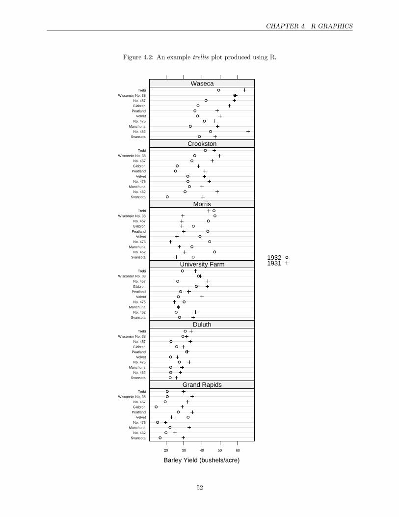
CHAPTER 4. R GRAPHICS
Figure 4.2: An example trellis plot produced using R.
Barley Yield (bushels/acre)
Svansota
No. 462
Manchuria
No. 475
Velvet
Peatland
Glabron
No. 457
Wisconsin No. 38
Trebi
20 30 40 50 60
●
●
●
●
●
●
●
●
●
●
Grand RapidsSvansota
No. 462
Manchuria
No. 475
Velvet
Peatland
Glabron
No. 457
Wisconsin No. 38
Trebi
●
●
●
●
●
●
●
●
●
●
DuluthSvansota
No. 462
Manchuria
No. 475
Velvet
Peatland
Glabron
No. 457
Wisconsin No. 38
Trebi
●
●
●
●
●
●
●
●
●
●
University FarmSvansota
No. 462
Manchuria
No. 475
Velvet
Peatland
Glabron
No. 457
Wisconsin No. 38
Trebi
●
●
●
●
●
●
●
●
●
●
MorrisSvansota
No. 462
Manchuria
No. 475
Velvet
Peatland
Glabron
No. 457
Wisconsin No. 38
Trebi
●
●
●
●
●
●
●
●
●
●
CrookstonSvansota
No. 462
Manchuria
No. 475
Velvet
Peatland
Glabron
No. 457
Wisconsin No. 38
Trebi
●
●
●
●
●
●
●
●
●
●
Waseca
19321931
●
52
CHAPTER 4. R GRAPHICS
that creates a ‘complete’ plot. This means that with high-level plotting functions, axes, labels and titles areautomatically generated, where appropriate, and unless you request otherwise. In addition, high-level plot-ting functions always start a new plot, erasing the current plot if necessary. Examples of high-level plottingfunctions are the (generic) plot(), hist() (histogram), and boxplot() functions. Sometimes, though, thehigh-level plotting function doesn’t produce exactly the kind of plot you desire. In this case, low-level plot-ting functions can be used to add more output (such as points, lines or text) to the current plot. Examples oflow-level plotting functions are the points(), legend(), and mtext() (margin text) functions. In actuality,some high-level plotting functions can also be forced to act like low-level ones. With all of this in mind, itis helpful to think of building your graph in layers until the desired final product is created. The ‘Plot fromscratch’ in Figure 4.1 is a good example of building a plot in layers – first the dotted and gray referencelines were added to the defined plotting grid; then the x-axis was added, then the rectangles, and then thetext. Because of this ‘painters model’, the only way to ‘edit’ graphical output is to modify and rerun the Rcode, or to produce output in a format that can be edited using third-party software. So, BE PATIENT.Creating the ‘final’ version of your graph takes a lot of trial-and-error.
ARGUMENTS OF PLOTTING FUNCTIONS: As we have seen with other non-plotting functions,all high- and low-level plotting functions have formal arguments that are specific to a particular function.For example, the boxplot() function has width= and boxwex= arguments (among others) for controlling thewidth of the boxes in the plot, and the barplot() function has a horiz= argument for controlling whetherbars are drawn horizontally rather than vertically. In turn, various aspects of the graphical output can bemodified or completely replaced. However, you are not limited to arguments that are specific to a singlehigh- or low-level plotting function.
For high-level plotting functions, in addition to function-specific arguments, there are several argumentsthat are ‘standard’ in the sense that many high-level plotting functions will accept them. Specifically, mosthigh-level plotting functions will accept graphical parameter arguments that control such things as the ap-pearance of axes and labels, and the range of the axes scales. It is usually possible to modify the defaultrange of the axes scales on a plot by specifying the xlim= and/or ylim= arguments in the high-level functioninvocation, which are each specified as two element vectors containing the minimum and maximum values(e.g., xlim = c(0, 50)). There is also a set of arguments for modifying the default labels (if any) on aplot: main= for a title, sub= for a sub-title, xlab= for an x-axis label, and ylab= for a y-axis label. Eachof these arguments is specified as a character string. The title specified with the main= argument (if any)is placed at the top of the plot in a large font, and the sub-title specified with the sub= argument is placedjust below the x-axis in a smaller font. Some high-level plotting functions have an axes= argument (bydefault TRUE), which allows you to suppress the drawing of the axes and therefore produce customized axesinstead. Lastly, some high-level plotting function have an add= argument (by default FALSE), which, if set toTRUE, forces the function to act as a low-level plotting, superimposing the high-level plot onto the current plot.
Lastly, most high- and low-level plotting functions will also appropriately accept graphical parameter argu-ments that control such things as data symbols, axes, color, line type and width, and text font, justification,magnification, and rotation. In many cases though, these arguments are not given as explicitly named ar-guments to the high- or low-level function, but are accepted instead via a ... argument. These unspecifiedgraphical parameter arguments are a subset of the formal arguments of the par() function.
THE par() FUNCTION: The par() function is the main function used to access and modify numerousgraphical parameters. These parameters describe and control things such as the general appearance ofgraphical output (the colors and line types that are used to draw lines, the fonts that are used to draw text,etc.), but also describe and control such things as the size and placement of the plot regions and coordinatesystems. Invoking the par() function with no specified arguments will result in a complete listing of thegraphical parameters you may set and their current values. Specific graphical parameters can be queried bysupplying specific parameter names as arguments to the par() function. For example, the following codequeries the current values of the col= (color) and lty= (line type) parameters.
> par(c("col", "lty"))
53
CHAPTER 4. R GRAPHICS
$col[1] "black"
$lty[1] "solid"
And specific parameters can be modified by specifying a value via an argument with the appropriate pa-rameter name. For example, par(col = "red", lty = "dashed") sets new values for the col= and lty=arguments.
As mentioned, a specific subset of the par() function’s arguments can be set not only via the par() function,but can also be used as arguments to other high- and low-level plotting functions, where appropriate. Thesearguments include:
Group Argument DescriptionPoints pch= data symbol type (‘point character’)
type= type of plot (points, lines, both)Lines lty= line type (solid, dashed)
lwd= line widthText adj= justification of text
cex= size of text (magnification multiplier)font= font face (bold, italic) for textlas= rotation of text in margins
Color col= color of lines and data symbols
On the other hand, some graphics settings can be set only via the par() function, which include:
Group Argument DescriptionPlotting regions & Margins mar= size of figure margins (lines of text)
oma= size of outer margins (lines of text)Multiple plots mfrow= number of figures on a pageOverlaying output new= has a new plot been started?
See the par() function’s help file and the second document for a complete list and detailed descriptionof the available arguments. We will be using many of these arguments soon.
TEMPORARY/PERSISTENT ALTERATIONS OF GRAPHICAL PARAMETERS: Modifyingtraditional graphical parameters via the par() function has a persistent effect. That is, parameters specifiedin this way hold until a different parameter is specified via another par() function invocation. In otherwords, when a graphical parameter is modified using the par() function, all future invocations of high- andlow-level plotting functions will be appropriately affected by that new parameter, as if you set a ‘default’value for that parameter. This ‘default’ parameter will be used by all subsequent plotting functions unlessan alternative is given. In contrast, graphical parameters may also be temporarily modified by specifyinga new value in the invocation of a high- or low-level plotting function such as the plot() function. Thefollowing code demonstrates this idea. First, the line type is permanently set as dashed using the par()function. Therefore, in the subsequent line plot (plot(y, type = "l")), the line will be dashed. However,in the next plot, a temporary line type parameter of lty = "solid" is specified, which causes the line inthis plot to be solid. Lastly, when the third plot is drawn, the permanent line type parameter of lty ="dashed" comes back into effect and thus the line is again dashed.
> y <- rnorm(20)> par(lty = "dashed")
54
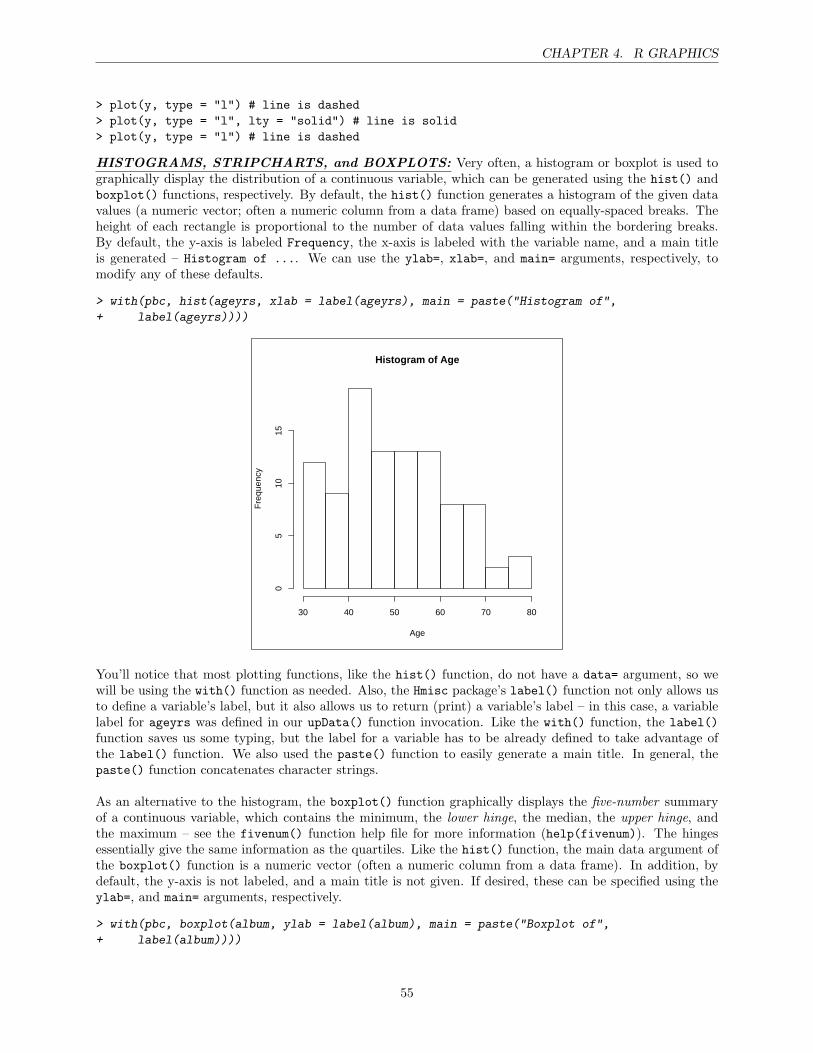
CHAPTER 4. R GRAPHICS
> plot(y, type = "l") # line is dashed> plot(y, type = "l", lty = "solid") # line is solid> plot(y, type = "l") # line is dashed
HISTOGRAMS, STRIPCHARTS, and BOXPLOTS: Very often, a histogram or boxplot is used tographically display the distribution of a continuous variable, which can be generated using the hist() andboxplot() functions, respectively. By default, the hist() function generates a histogram of the given datavalues (a numeric vector; often a numeric column from a data frame) based on equally-spaced breaks. Theheight of each rectangle is proportional to the number of data values falling within the bordering breaks.By default, the y-axis is labeled Frequency, the x-axis is labeled with the variable name, and a main titleis generated – Histogram of .... We can use the ylab=, xlab=, and main= arguments, respectively, tomodify any of these defaults.
> with(pbc, hist(ageyrs, xlab = label(ageyrs), main = paste("Histogram of",
+ label(ageyrs))))
Histogram of Age
Age
Fre
quen
cy
30 40 50 60 70 80
05
1015
You’ll notice that most plotting functions, like the hist() function, do not have a data= argument, so wewill be using the with() function as needed. Also, the Hmisc package’s label() function not only allows usto define a variable’s label, but it also allows us to return (print) a variable’s label – in this case, a variablelabel for ageyrs was defined in our upData() function invocation. Like the with() function, the label()function saves us some typing, but the label for a variable has to be already defined to take advantage ofthe label() function. We also used the paste() function to easily generate a main title. In general, thepaste() function concatenates character strings.
As an alternative to the histogram, the boxplot() function graphically displays the five-number summaryof a continuous variable, which contains the minimum, the lower hinge, the median, the upper hinge, andthe maximum – see the fivenum() function help file for more information (help(fivenum)). The hingesessentially give the same information as the quartiles. Like the hist() function, the main data argument ofthe boxplot() function is a numeric vector (often a numeric column from a data frame). In addition, bydefault, the y-axis is not labeled, and a main title is not given. If desired, these can be specified using theylab=, and main= arguments, respectively.
> with(pbc, boxplot(album, ylab = label(album), main = paste("Boxplot of",
+ label(album))))
55
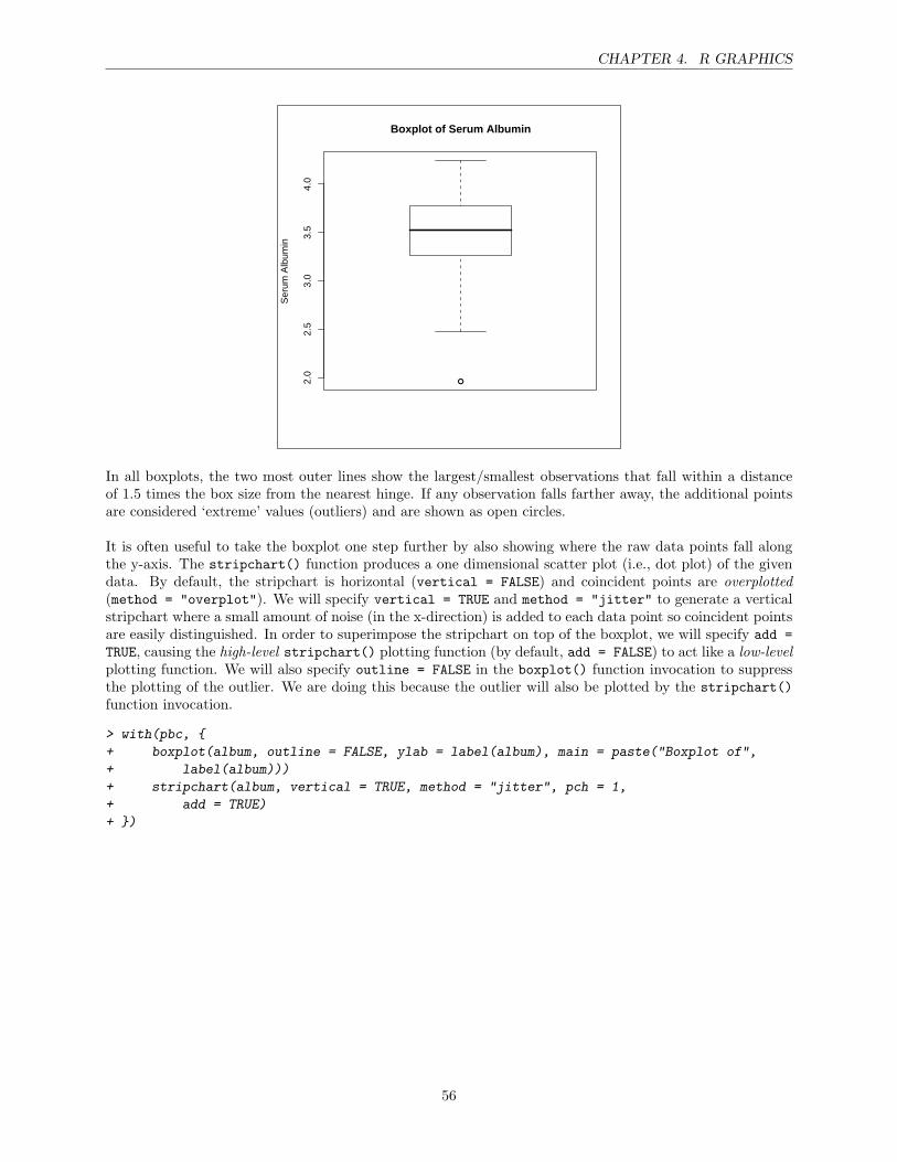
CHAPTER 4. R GRAPHICS
●2.0
2.5
3.0
3.5
4.0
Boxplot of Serum Albumin
Ser
um A
lbum
in
In all boxplots, the two most outer lines show the largest/smallest observations that fall within a distanceof 1.5 times the box size from the nearest hinge. If any observation falls farther away, the additional pointsare considered ‘extreme’ values (outliers) and are shown as open circles.
It is often useful to take the boxplot one step further by also showing where the raw data points fall alongthe y-axis. The stripchart() function produces a one dimensional scatter plot (i.e., dot plot) of the givendata. By default, the stripchart is horizontal (vertical = FALSE) and coincident points are overplotted(method = "overplot"). We will specify vertical = TRUE and method = "jitter" to generate a verticalstripchart where a small amount of noise (in the x-direction) is added to each data point so coincident pointsare easily distinguished. In order to superimpose the stripchart on top of the boxplot, we will specify add =TRUE, causing the high-level stripchart() plotting function (by default, add = FALSE) to act like a low-levelplotting function. We will also specify outline = FALSE in the boxplot() function invocation to suppressthe plotting of the outlier. We are doing this because the outlier will also be plotted by the stripchart()function invocation.
> with(pbc, {
+ boxplot(album, outline = FALSE, ylab = label(album), main = paste("Boxplot of",
+ label(album)))
+ stripchart(album, vertical = TRUE, method = "jitter", pch = 1,
+ add = TRUE)
+ })
56
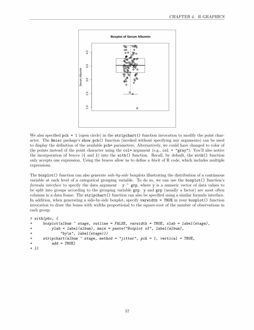
CHAPTER 4. R GRAPHICS
2.0
2.5
3.0
3.5
4.0
Boxplot of Serum Albumin
Ser
um A
lbum
in
●
●
●
●
●
●
●
●
●
●
●
●
●
●
●
●
●
●
●
●
●
●●
●
●
●
●
●
●
●
●
●
●
●
●●
●
●
●
●
●
●
●
●
● ●
●
●
●
● ●
●
●
●
●
●
●
●
●
●
● ●
●
●
●
●
●
●
●
●
●
●
●
●
●
●
●
●
●
●
●
●
●
●
●
●
●
●
●
●
●
●
●
●●
●
●
●
●
●
We also specified pch = 1 (open circle) in the stripchart() function invocation to modify the point char-acter. The Hmisc package’s show.pch() function (invoked without specifying any arguments) can be usedto display the definition of the available pch= parameters. Alternatively, we could have changed to color ofthe points instead of the point character using the col= argument (e.g., col = "gray"). You’ll also noticethe incorporation of braces ({ and }) into the with() function. Recall, by default, the with() functiononly accepts one expression. Using the braces allow us to define a block of R code, which includes multipleexpressions.
The boxplot() function can also generate side-by-side boxplots illustrating the distribution of a continuousvariable at each level of a categorical grouping variable. To do so, we can use the boxplot() function’sformula interface to specify the data argument – y ~ grp, where y is a numeric vector of data values tobe split into groups according to the grouping variable grp. y and grp (usually a factor) are most oftencolumns in a data frame. The stripchart() function can also be specified using a similar formula interface.In addition, when generating a side-by-side boxplot, specify varwidth = TRUE in your boxplot() functioninvocation to draw the boxes with widths proportional to the square-root of the number of observations ineach group.
> with(pbc, {
+ boxplot(album ~ stage, outline = FALSE, varwidth = TRUE, xlab = label(stage),
+ ylab = label(album), main = paste("Boxplot of", label(album),
+ "by\n", label(stage)))
+ stripchart(album ~ stage, method = "jitter", pch = 1, vertical = TRUE,
+ add = TRUE)
+ })
57
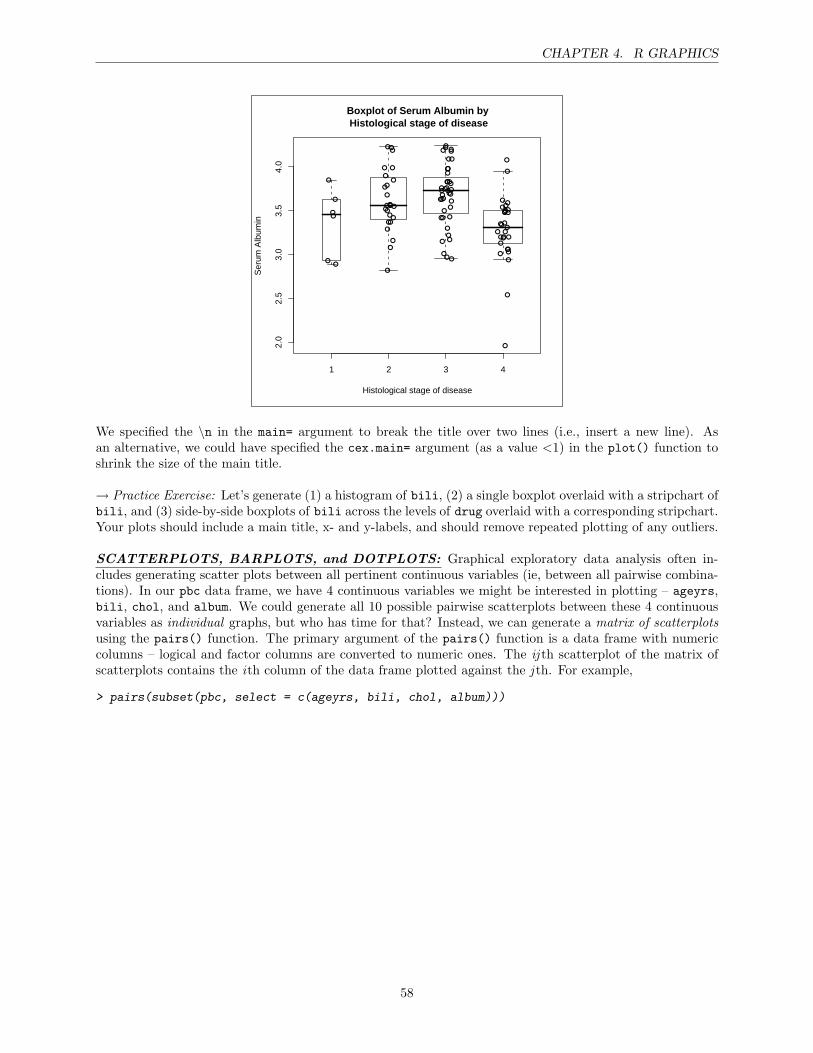
CHAPTER 4. R GRAPHICS
1 2 3 4
2.0
2.5
3.0
3.5
4.0
Boxplot of Serum Albumin by Histological stage of disease
Histological stage of disease
Ser
um A
lbum
in
●
●
●
●
●
●
●
●
●
●
●
●●
●
●
●
●
●
●
●
●
●
●
●
●
●
●
●
●
●
●
● ●
●
●
●
●
●
●
●
●●
●
●
●
●
●
●
●
●
●
●
●
●
●
●
●
●
●
●
●
●
●●
●
●
●
●
●
●
●
●
●
●
●
●
●
●
●
●
●
●
●
● ●●
●
●
●
●
●
●
●
●●
●
●
●
We specified the \n in the main= argument to break the title over two lines (i.e., insert a new line). Asan alternative, we could have specified the cex.main= argument (as a value <1) in the plot() function toshrink the size of the main title.
→ Practice Exercise: Let’s generate (1) a histogram of bili, (2) a single boxplot overlaid with a stripchart ofbili, and (3) side-by-side boxplots of bili across the levels of drug overlaid with a corresponding stripchart.Your plots should include a main title, x- and y-labels, and should remove repeated plotting of any outliers.
SCATTERPLOTS, BARPLOTS, and DOTPLOTS: Graphical exploratory data analysis often in-cludes generating scatter plots between all pertinent continuous variables (ie, between all pairwise combina-tions). In our pbc data frame, we have 4 continuous variables we might be interested in plotting – ageyrs,bili, chol, and album. We could generate all 10 possible pairwise scatterplots between these 4 continuousvariables as individual graphs, but who has time for that? Instead, we can generate a matrix of scatterplotsusing the pairs() function. The primary argument of the pairs() function is a data frame with numericcolumns – logical and factor columns are converted to numeric ones. The ij th scatterplot of the matrix ofscatterplots contains the ith column of the data frame plotted against the j th. For example,
> pairs(subset(pbc, select = c(ageyrs, bili, chol, album)))
58
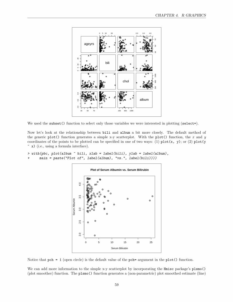
CHAPTER 4. R GRAPHICS
ageyrs
0 5 10 20
●
●
●
●
●
●
●●
●
●
●●
●
●
●
●
●
●
●
●
●●●
●
●
●
●
●
●
●
●
●
●
●
●
● ●
●
●
●
●
●
●
●●
●
●
●
●
●
●
●●
●
●
●
●
●
●
●●
●
●
●
●
●
●
●
●
●
●
●
●
●
●
●
●
●●
●
●
●
●
●
●
●
●
●
●
● ●
●
●
●●●
●
●
●●
●
●
●
●
●
●
●
●
● ●
●
●
●
●
●
●
●
●●●
●
●
●
●
●
●
●
●
●
●
●
●
●
●
●
●
●●
●
●
●
●
●
●
●●
●
●
●
●
●
●
●●
●
●
●
●
●
●
●
●
●
●
●
●
●
●
2.0 3.0 4.0
3050
70
●
●
●
●
●
●
● ●
●
●
●●
●
●
●
●
●
●
●
●
●●●
●
●
●
●
●
●
●
●
●
●
●
●
●●
●
●
●
●
●
●
●●
●
●
●
●
●
●
●●
●
●
●
●
●
●
● ●
●
●
●
●
●
●
●
●
●
●
●
●
●
●
●
●
●●
●
●
●
●
●
●
●
●
●
●
●●
●
●
●●
●
●
●
● ●
05
1020
●
●●●
●
●●
● ● ●●● ●
●
●●● ●●
●●
●
●
●●
●
●● ●
● ●●●
●
●
●
●
●●
●●
●
●
●●
●
●
●
● ●●
● ●
●
● ●●●
●
●●
●● ● ●●
●
●
●● ● ●●
●
●
●● ●●
●
●
●
●●● ●
●
●● ●
●
●●
●●●●● ●●
bili
●
●● ●
●
●
●●● ●●
●
●● ●● ●●
●
●
●●
●
●●●
●●●
●
●
●●●
●
●
●●
●
●
●
●●●
●●
●
●● ●●
●
●●
●●●●●
●
●
●●●●●
●
●
●
●● ●
●
● ●
● ●● ●● ●
●
●● ●● ●
●●
●
●
●●
●
●●●
●● ●●
●
●
●
●
●●
●●
●
●
●●
●
●
●
●●●
●●
●
● ●●●
●
● ●
●● ●●●
●
●
●● ●●●
●
●
● ●● ●
●
●
●
●● ●●
●
●●●
●
●●
●●●
●●● ●
●
●
●
●
●●
● ●
●
● ●
●
●●
●
●
●
●
●
●
●●
●
●
●
●● ●
●
●
●
●
●
●
●
●
●
●
●●
●●●
●●●
●
●●
●
●●
●● ●
● ● ●●
●
●
●
●
● ●● ●
●
●
●
●
●
●●
●●
●
●●
●
● ●
●
●
●
●
●
●
●●
●
●
●
●●●
●
●
●
●
●
●
●
●
●
●
●●
●●●
● ●●
●
●●
●
●●
●●●
●●●●
●
●
●
●
●●●●
● chol
200
600
1000
●
●
●
●
●●
●●
●
● ●
●
●●
●
●
●
●
●
●
●●
●
●
●
●●●
●
●
●
●
●
●
●
●
●
●
●●
● ●●
● ●●
●
●●
●
●●
● ●●
● ●●●
●
●
●
●
●●●●
●
30 50 70
2.0
3.0
4.0
●
●
●●
●
●
●
●●
●
●
●
●●
●
●
●
●
●
●
●
●●
●
●
●●
●●
●
●
●
●
●
●●
●
●
●
●
●●
●
●
● ●●
●
●●●
●
●
●
●
●
●
●
●
●
● ●
●
●●
●
●
●●
●
●
●●
●
●
●
●
●
●
●●
●
●
●
●
●
●●
●
●●
●
●
●●
●
●●
●
●
●
●
●●
●
●
●
●●
●
●
●
●●
●
●
●
●
●
●
●
●●
●
●
●●
●●
●
●
●
●
●
●●
●
●
●
●
●●
●
●
● ●●
●
●●●
●
●
●
●
●
●
●
●
●
●●
●
●●
●
●
●●
●
●
●●
●
●
●
●
●
●
●●
●
●
●
●
●
●●
●
●●
●
●
●●
●
●●
●
●
200 600 1000
●
●
●●
●
●
●
●
●
●
●●
●
●
●
●
●
●
●●
●
●
●●
●●
●
●
●
●
● ●
●
●●
●
●
● ●●
●
●●●
●
●
●
●
●
●
●
●
●
●●
●
●●
●
●
●●
●
●
●●
●
●
album
We used the subset() function to select only those variables we were interested in plotting (select=).
Now let’s look at the relationship between bili and album a bit more closely. The default method ofthe generic plot() function generates a simple x-y scatterplot. With the plot() function, the x and ycoordinates of the points to be plotted can be specified in one of two ways: (1) plot(x, y); or (2) plot(y~ x) (i.e., using a formula interface).
> with(pbc, plot(album ~ bili, xlab = label(bili), ylab = label(album),
+ main = paste("Plot of", label(album), "vs.", label(bili))))
●
●
●
●
●
●
●
●
●
●
●
●
●
●
●
●
●
●
●
●
●
●●
●
●
●
●
●
●
●
●
●
●
●
●●
●
●
●
●
●
●
●
●
● ●
●
●
●
●●
●
●
●
●
●
●
●
●
●
●●
●
●
●
●
●
●
●
●
●
●
●
●
●
●
●
●
●
●
●
●
●
●
●
●
●
●
●
●
●
●
●
●●
●
●
●
●
●
0 5 10 15 20 25
2.0
2.5
3.0
3.5
4.0
Plot of Serum Albumin vs. Serum Bilirubin
Serum Bilirubin
Ser
um A
lbum
in
Notice that pch = 1 (open circle) is the default value of the pch= argument in the plot() function.
We can add more information to the simple x-y scatterplot by incorporating the Hmisc package’s plsmo()(plot smoother) function. The plsmo() function generates a (non-parametric) plot smoothed estimate (line)
59
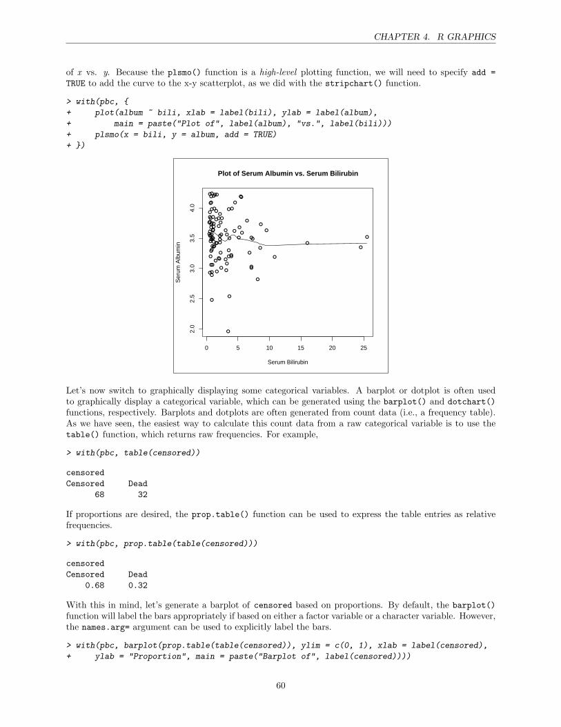
CHAPTER 4. R GRAPHICS
of x vs. y. Because the plsmo() function is a high-level plotting function, we will need to specify add =TRUE to add the curve to the x-y scatterplot, as we did with the stripchart() function.
> with(pbc, {
+ plot(album ~ bili, xlab = label(bili), ylab = label(album),
+ main = paste("Plot of", label(album), "vs.", label(bili)))
+ plsmo(x = bili, y = album, add = TRUE)
+ })
●
●
●
●
●
●
●
●
●
●
●
●
●
●
●
●
●
●
●
●
●
●●
●
●
●
●
●
●
●
●
●
●
●
●●
●
●
●
●
●
●
●
●
● ●
●
●
●
●●
●
●
●
●
●
●
●
●
●
●●
●
●
●
●
●
●
●
●
●
●
●
●
●
●
●
●
●
●
●
●
●
●
●
●
●
●
●
●
●
●
●
●●
●
●
●
●
●
0 5 10 15 20 25
2.0
2.5
3.0
3.5
4.0
Plot of Serum Albumin vs. Serum Bilirubin
Serum Bilirubin
Ser
um A
lbum
in
Let’s now switch to graphically displaying some categorical variables. A barplot or dotplot is often usedto graphically display a categorical variable, which can be generated using the barplot() and dotchart()functions, respectively. Barplots and dotplots are often generated from count data (i.e., a frequency table).As we have seen, the easiest way to calculate this count data from a raw categorical variable is to use thetable() function, which returns raw frequencies. For example,
> with(pbc, table(censored))
censoredCensored Dead
68 32
If proportions are desired, the prop.table() function can be used to express the table entries as relativefrequencies.
> with(pbc, prop.table(table(censored)))
censoredCensored Dead
0.68 0.32
With this in mind, let’s generate a barplot of censored based on proportions. By default, the barplot()function will label the bars appropriately if based on either a factor variable or a character variable. However,the names.arg= argument can be used to explicitly label the bars.
> with(pbc, barplot(prop.table(table(censored)), ylim = c(0, 1), xlab = label(censored),
+ ylab = "Proportion", main = paste("Barplot of", label(censored))))
60
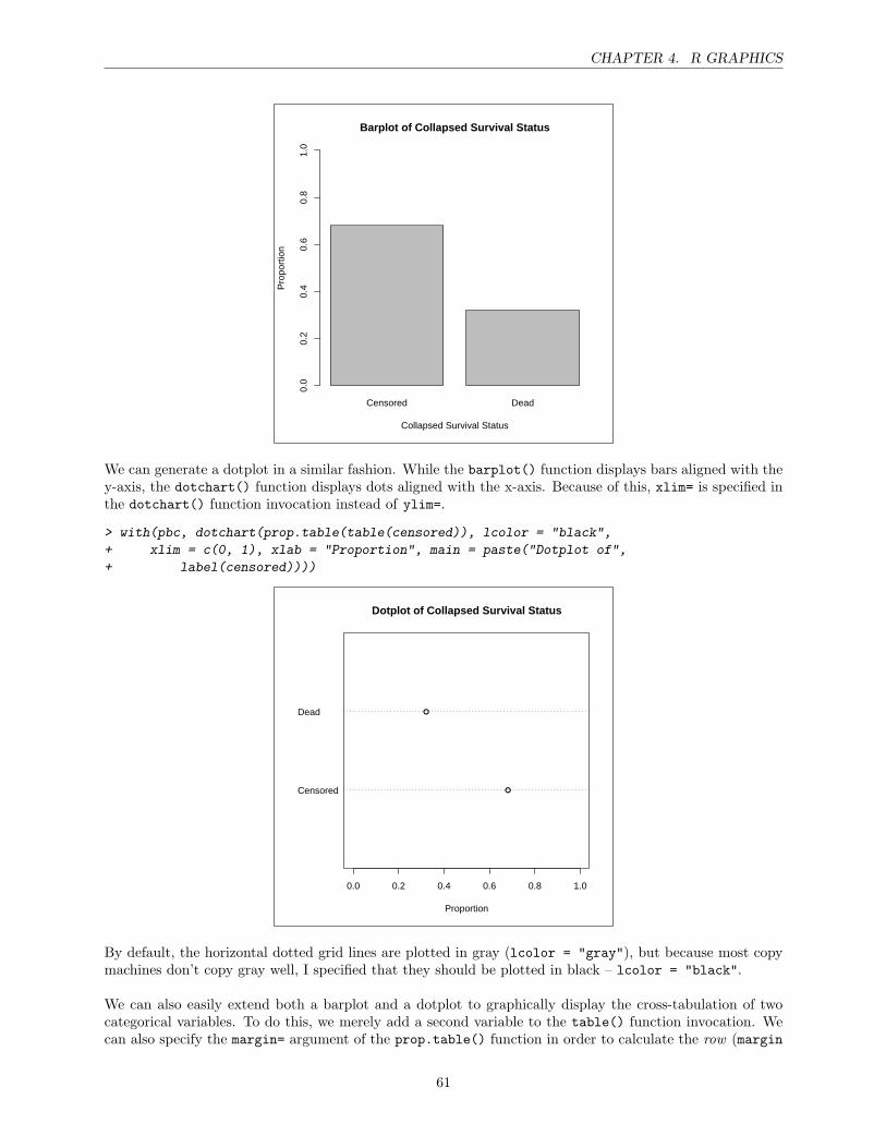
CHAPTER 4. R GRAPHICS
Censored Dead
Barplot of Collapsed Survival Status
Collapsed Survival Status
Pro
port
ion
0.0
0.2
0.4
0.6
0.8
1.0
We can generate a dotplot in a similar fashion. While the barplot() function displays bars aligned with they-axis, the dotchart() function displays dots aligned with the x-axis. Because of this, xlim= is specified inthe dotchart() function invocation instead of ylim=.
> with(pbc, dotchart(prop.table(table(censored)), lcolor = "black",
+ xlim = c(0, 1), xlab = "Proportion", main = paste("Dotplot of",
+ label(censored))))
Censored
Dead
●
●
0.0 0.2 0.4 0.6 0.8 1.0
Dotplot of Collapsed Survival Status
Proportion
By default, the horizontal dotted grid lines are plotted in gray (lcolor = "gray"), but because most copymachines don’t copy gray well, I specified that they should be plotted in black – lcolor = "black".
We can also easily extend both a barplot and a dotplot to graphically display the cross-tabulation of twocategorical variables. To do this, we merely add a second variable to the table() function invocation. Wecan also specify the margin= argument of the prop.table() function in order to calculate the row (margin
61
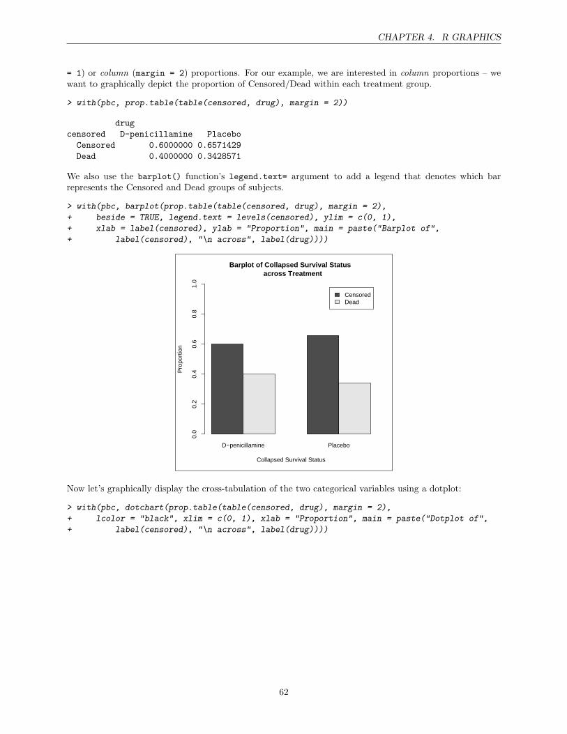
CHAPTER 4. R GRAPHICS
= 1) or column (margin = 2) proportions. For our example, we are interested in column proportions – wewant to graphically depict the proportion of Censored/Dead within each treatment group.
> with(pbc, prop.table(table(censored, drug), margin = 2))
drugcensored D-penicillamine PlaceboCensored 0.6000000 0.6571429Dead 0.4000000 0.3428571
We also use the barplot() function’s legend.text= argument to add a legend that denotes which barrepresents the Censored and Dead groups of subjects.
> with(pbc, barplot(prop.table(table(censored, drug), margin = 2),
+ beside = TRUE, legend.text = levels(censored), ylim = c(0, 1),
+ xlab = label(censored), ylab = "Proportion", main = paste("Barplot of",
+ label(censored), "\n across", label(drug))))
D−penicillamine Placebo
CensoredDead
Barplot of Collapsed Survival Status across Treatment
Collapsed Survival Status
Pro
port
ion
0.0
0.2
0.4
0.6
0.8
1.0
Now let’s graphically display the cross-tabulation of the two categorical variables using a dotplot:
> with(pbc, dotchart(prop.table(table(censored, drug), margin = 2),
+ lcolor = "black", xlim = c(0, 1), xlab = "Proportion", main = paste("Dotplot of",
+ label(censored), "\n across", label(drug))))
62
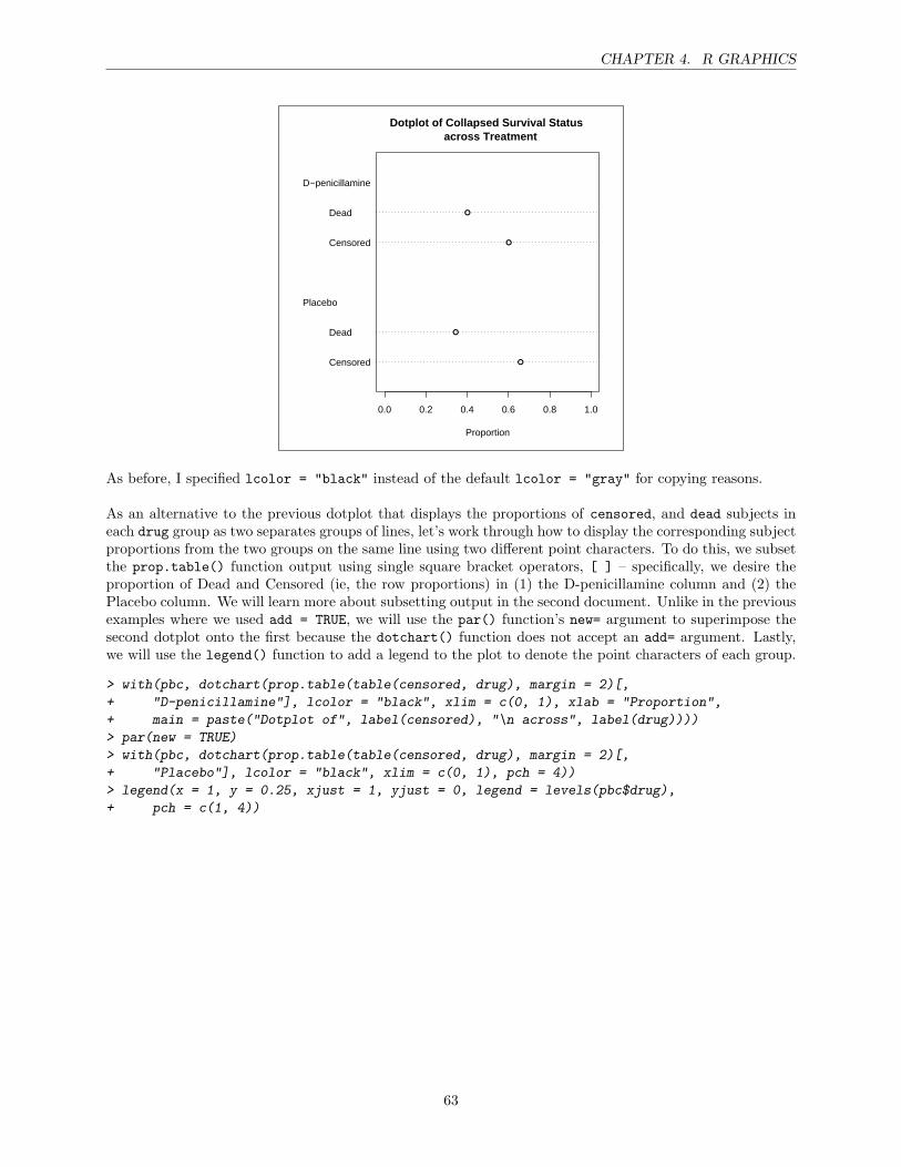
CHAPTER 4. R GRAPHICS
Censored
Dead
Censored
Dead
●
●
●
●
D−penicillamine
Placebo
0.0 0.2 0.4 0.6 0.8 1.0
Dotplot of Collapsed Survival Status across Treatment
Proportion
As before, I specified lcolor = "black" instead of the default lcolor = "gray" for copying reasons.
As an alternative to the previous dotplot that displays the proportions of censored, and dead subjects ineach drug group as two separates groups of lines, let’s work through how to display the corresponding subjectproportions from the two groups on the same line using two different point characters. To do this, we subsetthe prop.table() function output using single square bracket operators, [ ] – specifically, we desire theproportion of Dead and Censored (ie, the row proportions) in (1) the D-penicillamine column and (2) thePlacebo column. We will learn more about subsetting output in the second document. Unlike in the previousexamples where we used add = TRUE, we will use the par() function’s new= argument to superimpose thesecond dotplot onto the first because the dotchart() function does not accept an add= argument. Lastly,we will use the legend() function to add a legend to the plot to denote the point characters of each group.
> with(pbc, dotchart(prop.table(table(censored, drug), margin = 2)[,
+ "D-penicillamine"], lcolor = "black", xlim = c(0, 1), xlab = "Proportion",
+ main = paste("Dotplot of", label(censored), "\n across", label(drug))))
> par(new = TRUE)
> with(pbc, dotchart(prop.table(table(censored, drug), margin = 2)[,
+ "Placebo"], lcolor = "black", xlim = c(0, 1), pch = 4))
> legend(x = 1, y = 0.25, xjust = 1, yjust = 0, legend = levels(pbc$drug),
+ pch = c(1, 4))
63
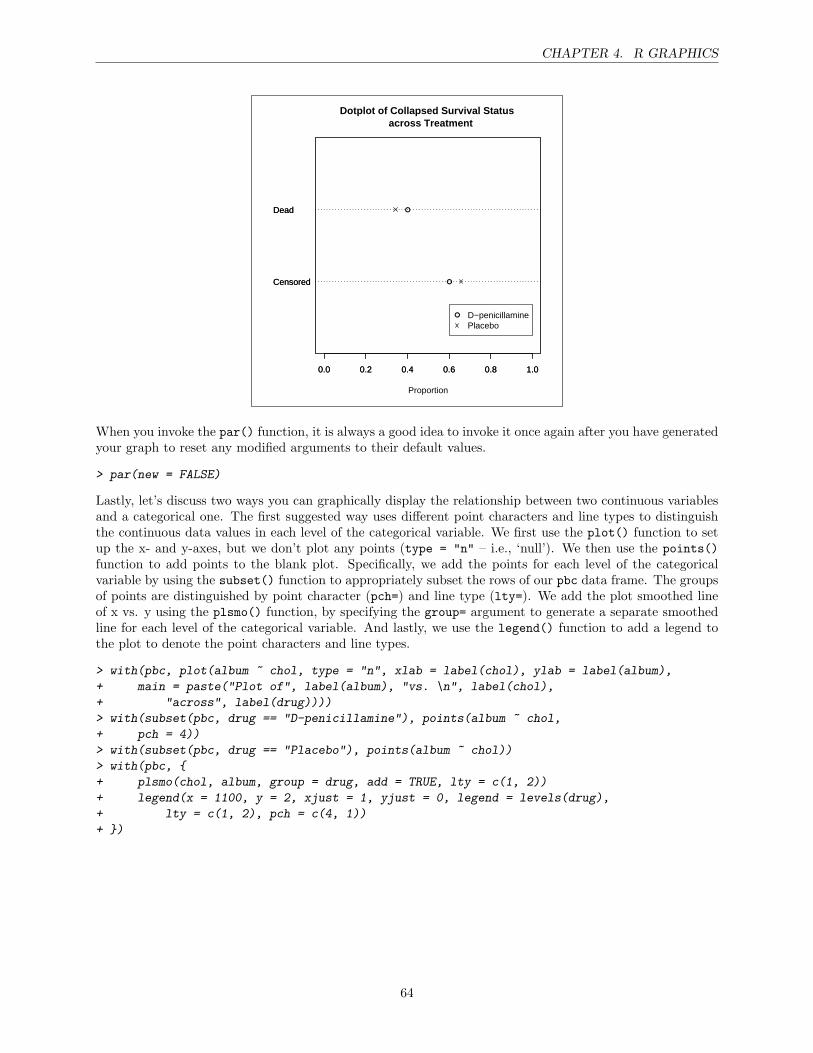
CHAPTER 4. R GRAPHICS
Censored
Dead
●
●
0.0 0.2 0.4 0.6 0.8 1.0
Dotplot of Collapsed Survival Status across Treatment
Proportion
Censored
Dead
0.0 0.2 0.4 0.6 0.8 1.0
● D−penicillaminePlacebo
When you invoke the par() function, it is always a good idea to invoke it once again after you have generatedyour graph to reset any modified arguments to their default values.
> par(new = FALSE)
Lastly, let’s discuss two ways you can graphically display the relationship between two continuous variablesand a categorical one. The first suggested way uses different point characters and line types to distinguishthe continuous data values in each level of the categorical variable. We first use the plot() function to setup the x- and y-axes, but we don’t plot any points (type = "n" – i.e., ‘null’). We then use the points()function to add points to the blank plot. Specifically, we add the points for each level of the categoricalvariable by using the subset() function to appropriately subset the rows of our pbc data frame. The groupsof points are distinguished by point character (pch=) and line type (lty=). We add the plot smoothed lineof x vs. y using the plsmo() function, by specifying the group= argument to generate a separate smoothedline for each level of the categorical variable. And lastly, we use the legend() function to add a legend tothe plot to denote the point characters and line types.
> with(pbc, plot(album ~ chol, type = "n", xlab = label(chol), ylab = label(album),
+ main = paste("Plot of", label(album), "vs. \n", label(chol),
+ "across", label(drug))))
> with(subset(pbc, drug == "D-penicillamine"), points(album ~ chol,
+ pch = 4))
> with(subset(pbc, drug == "Placebo"), points(album ~ chol))
> with(pbc, {
+ plsmo(chol, album, group = drug, add = TRUE, lty = c(1, 2))
+ legend(x = 1100, y = 2, xjust = 1, yjust = 0, legend = levels(drug),
+ lty = c(1, 2), pch = c(4, 1))
+ })
64
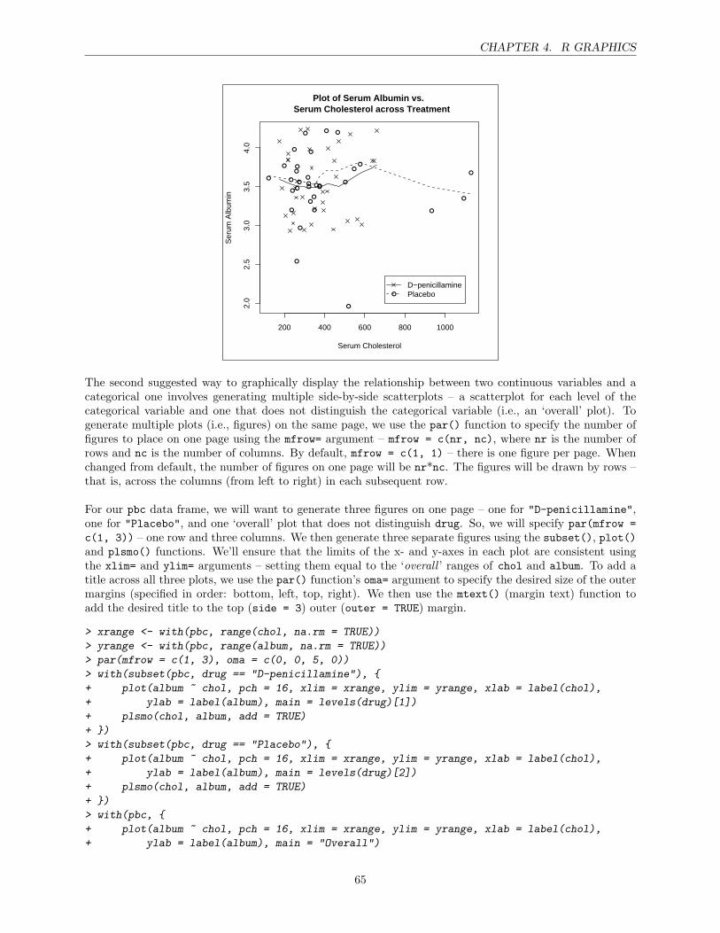
CHAPTER 4. R GRAPHICS
200 400 600 800 1000
2.0
2.5
3.0
3.5
4.0
Plot of Serum Albumin vs. Serum Cholesterol across Treatment
Serum Cholesterol
Ser
um A
lbum
in
●
●
●
●
●
●
●
●
●
●
●
●
●●
●
●
●●
●
●
●
●
●
●
●●
●●
●
●
●
●
●
D−penicillaminePlacebo
The second suggested way to graphically display the relationship between two continuous variables and acategorical one involves generating multiple side-by-side scatterplots – a scatterplot for each level of thecategorical variable and one that does not distinguish the categorical variable (i.e., an ‘overall’ plot). Togenerate multiple plots (i.e., figures) on the same page, we use the par() function to specify the number offigures to place on one page using the mfrow= argument – mfrow = c(nr, nc), where nr is the number ofrows and nc is the number of columns. By default, mfrow = c(1, 1) – there is one figure per page. Whenchanged from default, the number of figures on one page will be nr*nc. The figures will be drawn by rows –that is, across the columns (from left to right) in each subsequent row.
For our pbc data frame, we will want to generate three figures on one page – one for "D-penicillamine",one for "Placebo", and one ‘overall’ plot that does not distinguish drug. So, we will specify par(mfrow =c(1, 3)) – one row and three columns. We then generate three separate figures using the subset(), plot()and plsmo() functions. We’ll ensure that the limits of the x- and y-axes in each plot are consistent usingthe xlim= and ylim= arguments – setting them equal to the ‘overall ’ ranges of chol and album. To add atitle across all three plots, we use the par() function’s oma= argument to specify the desired size of the outermargins (specified in order: bottom, left, top, right). We then use the mtext() (margin text) function toadd the desired title to the top (side = 3) outer (outer = TRUE) margin.
> xrange <- with(pbc, range(chol, na.rm = TRUE))
> yrange <- with(pbc, range(album, na.rm = TRUE))
> par(mfrow = c(1, 3), oma = c(0, 0, 5, 0))
> with(subset(pbc, drug == "D-penicillamine"), {
+ plot(album ~ chol, pch = 16, xlim = xrange, ylim = yrange, xlab = label(chol),
+ ylab = label(album), main = levels(drug)[1])
+ plsmo(chol, album, add = TRUE)
+ })
> with(subset(pbc, drug == "Placebo"), {
+ plot(album ~ chol, pch = 16, xlim = xrange, ylim = yrange, xlab = label(chol),
+ ylab = label(album), main = levels(drug)[2])
+ plsmo(chol, album, add = TRUE)
+ })
> with(pbc, {
+ plot(album ~ chol, pch = 16, xlim = xrange, ylim = yrange, xlab = label(chol),
+ ylab = label(album), main = "Overall")
65
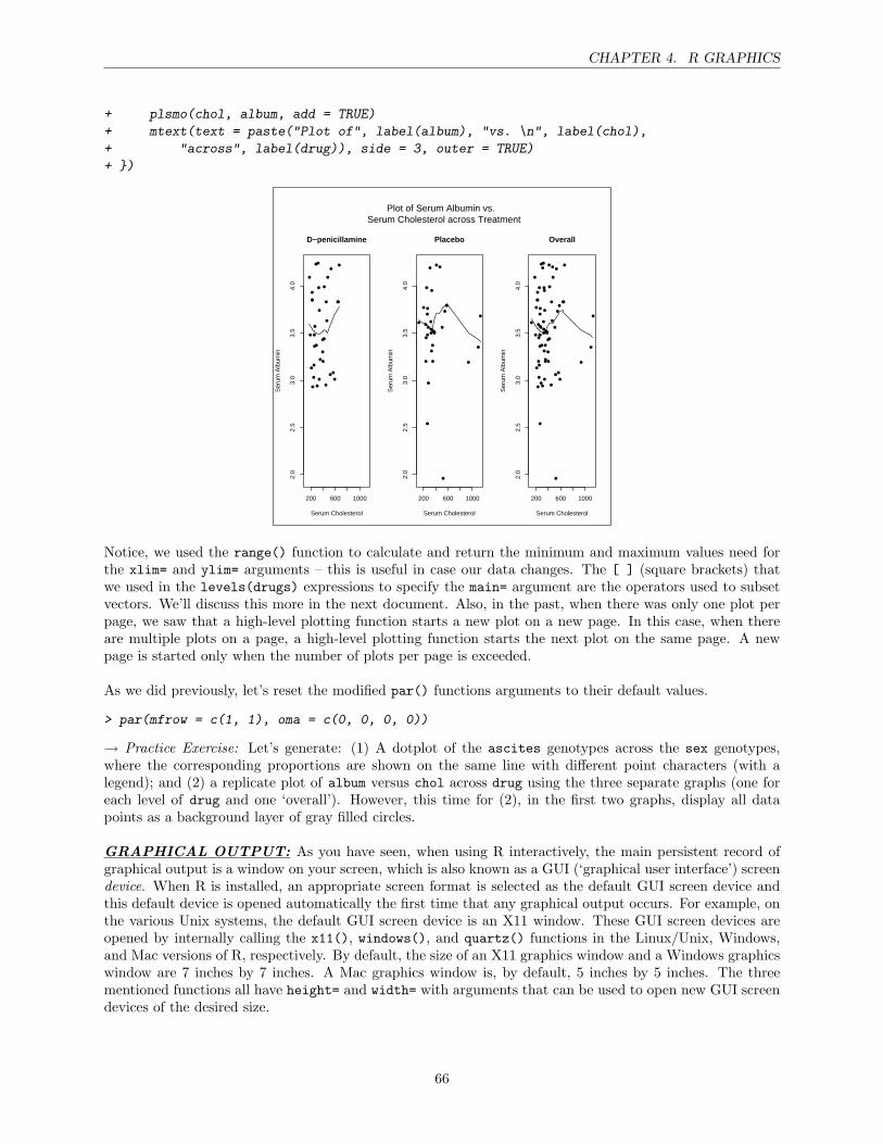
CHAPTER 4. R GRAPHICS
+ plsmo(chol, album, add = TRUE)
+ mtext(text = paste("Plot of", label(album), "vs. \n", label(chol),
+ "across", label(drug)), side = 3, outer = TRUE)
+ })
●
●
●
●
●
●
●
●
●
●
●
●
●
●
●
●
●
●
●
●
●
●
●●
●
●
●
●
●
●
●
●
●
●
●
●
200 600 1000
2.0
2.5
3.0
3.5
4.0
D−penicillamine
Serum Cholesterol
Ser
um A
lbum
in
●
●
●
●
●
●
●
●
●
●
●
●
●●
●
●
●●
●
●
●
●
●
●
●●
●●
●
●
●
●
200 600 1000
2.0
2.5
3.0
3.5
4.0
Placebo
Serum Cholesterol
Ser
um A
lbum
in
●
●
●
●
●
●
●
●
●
●
●
●
●
●
●
●
●
●
●●
●
●
●
●
●
●
●
●
●
●
●●
●
●
●
●
●
● ●
●
●
●
●●
●
●
●
●
●
●
●
●
●
●●
●
●
●
●
●
●
●
●
●
●
●
●
●
200 600 1000
2.0
2.5
3.0
3.5
4.0
Overall
Serum Cholesterol
Ser
um A
lbum
in
Plot of Serum Albumin vs. Serum Cholesterol across Treatment
Notice, we used the range() function to calculate and return the minimum and maximum values need forthe xlim= and ylim= arguments – this is useful in case our data changes. The [ ] (square brackets) thatwe used in the levels(drugs) expressions to specify the main= argument are the operators used to subsetvectors. We’ll discuss this more in the next document. Also, in the past, when there was only one plot perpage, we saw that a high-level plotting function starts a new plot on a new page. In this case, when thereare multiple plots on a page, a high-level plotting function starts the next plot on the same page. A newpage is started only when the number of plots per page is exceeded.
As we did previously, let’s reset the modified par() functions arguments to their default values.
> par(mfrow = c(1, 1), oma = c(0, 0, 0, 0))
→ Practice Exercise: Let’s generate: (1) A dotplot of the ascites genotypes across the sex genotypes,where the corresponding proportions are shown on the same line with different point characters (with alegend); and (2) a replicate plot of album versus chol across drug using the three separate graphs (one foreach level of drug and one ‘overall’). However, this time for (2), in the first two graphs, display all datapoints as a background layer of gray filled circles.
GRAPHICAL OUTPUT: As you have seen, when using R interactively, the main persistent record ofgraphical output is a window on your screen, which is also known as a GUI (‘graphical user interface’) screendevice. When R is installed, an appropriate screen format is selected as the default GUI screen device andthis default device is opened automatically the first time that any graphical output occurs. For example, onthe various Unix systems, the default GUI screen device is an X11 window. These GUI screen devices areopened by internally calling the x11(), windows(), and quartz() functions in the Linux/Unix, Windows,and Mac versions of R, respectively. By default, the size of an X11 graphics window and a Windows graphicswindow are 7 inches by 7 inches. A Mac graphics window is, by default, 5 inches by 5 inches. The threementioned functions all have height= and width= with arguments that can be used to open new GUI screendevices of the desired size.
66
CHAPTER 4. R GRAPHICS
In the Windows version of R, right-clicking on the graphics window offers you three options for outputtingany desired graph from R: (1) Copy your graph as either a metafile or a bitmap; (2) Save your graph aseither a metafile or postscript; and/or (3) Print your graph. For the Copy and Save options, it is very easyto then Paste or Insert, respectively, your graph into a Microsoft Word and/or Powerpoint document.
In any version of R, it is also possible to produce a file that contains your plot. Similar to the GUI screendevices, the graphical output can be directed to a particular file device, which dictates the output formatthat will be produced. And like the GUI screen devices, the file devices are controlled by specific functions,including the pdf() function that produces an Adobe PDF file. Like the GUI screen device functions, thesefile device functions allow you to specify things such as the name of the file and the size of the plot. Unlikesending graphical output to a window on your screen, directing graphical output to a file takes a few moresteps. A file device must be created or ‘opened to writing’ in order to receive graphical output by invokingthe desired file device function with at least the desired file name specified. Once you have opened the file towriting, you then execute all of your desired graphical function invocations. In turn, the specific file devicethat you opened converts the graphical function invocations from R (e.g., ‘draw a line’) into commandsthat the particular device can understand and your graphical output is generated. When you have finishedwriting the desired graphical output to a file, you then close the file to writing (and therefore close the filedevice) by invoking the dev.off() (‘device off’) function. For example, let’s write a simple scatterplot to aPDF file named myplot.pdf:
> pdf("myplot.pdf", height = 8.5, width = 11)> with(pbc, plot(ageyrs ~ chol,+ main = "Age (years) vs. Serum Chol",+ xlab = label(chol), ylab = label(ageyrs)))> dev.off()
In the previous code, we also specified that the plot should be in a landscape orientation (i.e., height <width), with a height of 8.5” and a width of 11.0”.
A THOUGHT TO END WITH: Keep in mind that there are always multiple ways of performing thesame task in R. And remember to read, read, read – read the documentation, including help files and theirexamples; read others’ code; and read the body of defined functions. Also, feel free to check out the website forthe weekly ‘R Clinic’ that I run at Vanderbilt University – http://biostat.mc.vanderbilt.edu/RClinic.It contains the ‘solutions’ to problems that various ‘R Clinic’ attendees have posed.
67