2

An Introduction to Support Vector Machines for Data

Mining

Robert Burbidge, Bernard Buxton

Computer Science Dept., UCL, Gower Street, WC1E 6BT, UK.

Abstract

With increasing amounts of data being generated by businesses and researchers there is a need

for fast, accurate and robust algorithms for data analysis. Improvements in databases

technology, computing performance and artificial intelligence have contributed to the

development of intelligent data analysis. The primary aim of data mining is to discover

patterns in the data that lead to better understanding of the data generating process and to

useful predictions. Examples of applications of data mining include detecting fraudulent

credit card transactions, character recognition in automated zip code reading, and predicting

compound activity in drug discovery. Real-world data sets are often characterized by having

large numbers of examples, e.g. billions of credit card transactions and potential ‘drug-like’

compounds; being highly unbalanced, e.g. most transactions are not fraudulent, most

compounds are not active against a given biological target; and, being corrupted by noise.

The relationship between predictive variables, e.g. physical descriptors, and the target concept,

e.g. compound activity, is often highly non-linear. One recent technique that has been

developed to address these issues is the support vector machine. The support vector machine

has been developed as robust tool for classification and regression in noisy, complex domains.

The two key features of support vector machines are generalization theory, which leads to a

principled way to choose an hypothesis; and, kernel functions, which introduce non-linearity

in the hypothesis space without explicitly requiring a non-linear algorithm. In this tutorial I

introduce support vector machines and highlight the advantages thereof over existing data

analysis techniques, also are noted some important points for the data mining practitioner who

wishes to use support vector machines.

Motivation

As John Denker has remarked ‘neural networks are the second best way of doing just

about anything’. The meaning behind this statement is that the best way of solving a

particular problem is to apply all available domain knowledge and spend a

considerable amount of time, money and effort in building a rule system that will give

the right answer. The second best way of doing anything is to learn from experience.

Given the increasing quantity of data for analysis and the variety and complexity of

data analysis problems being encountered in business, industry and research, it is

impractical to demand the best solution every time. The ultimate dream, of course is

to have available some intelligent agent that can pre-process your data, apply the

appropriate mathematical, statistical and artificial intelligence techniques, and then

provide a solution and an explanation. In the meantime we must be content with the

pieces of this automatic problem solver. It is the purpose of the data miner to use the

available tools to analyze data and provide a partial solution to a business problem.

The data mining process can be roughly separated into three activities: pre-processing,

modeling and prediction, and explaining. There is much overlap between these stages

and the process is far from linear. Here we concentrate on the central of these tasks,

3

in particular prediction. Machine learning in the general sense is described and the

problem of hypothesis selection detailed. The support vector machine (SVM) is then

introduced as a robust and principled way to choose an hypothesis. The SVM for

two-class classification is dealt with in detail and some practical issues discussed.

Finally, related algorithms for regression, novelty detection and other data mining

tasks are discussed.

Machine Learning

The general problem of machine learning is to search a, usually very large, space of

potential hypotheses to determine the one that will best fit the data and any prior

knowledge1. The data may be labelled or unlabelled. If labels are given then the

problem is one of supervised learning in that the true answer is known for a given set

of data. If the labels are categorical then the problem is one of classification, e.g.

predicting the species of a flower given petal and sepal measurements2. If the labels

are real-valued the problem is one of regression, e.g. predicting property values from

crime, pollution, etc. statistics3. If labels are not given then the problem is one of

unsupervised learning and the aim is characterize the structure of the data, e.g. by

identifying groups of examples in the data that are collectively similar to each other

and distinct from the other data.

Supervised Learning

Given some examples we wish to predict certain properties, in the case where there

are available a set of examples whose properties have already been characterized the

task is to learn the relationship between the two. One common early approach4 was to

present the examples in turn to a learner. The learner makes a prediction of the

property of interest, the correct answer is presented, and the learner adjusts its

hypothesis accordingly. This is known as learning with a teacher, or supervised

learning.

In supervised learning there is necessarily the assumption that the descriptors

available are in some related to a quantity of interest. For instance, suppose that a

bank wishes to detect fraudulent credit card transactions. In order to do this some

domain knowledge is required to identify factors that are likely to be indicative of

fraudulent use. These may include frequency of usage, amount of transaction,

spending patterns, type of business engaging in the transaction and so forth. These

variables are the predictive, or independent, variables x . It would be hoped that these

were in some way related to the target, or dependent, variable y . Deciding which

variables to use in a model is a very difficult problem in general; this is known as the

problem of feature selection and is NP-complete. Many methods exist for choosing

the predictive variables, if domain knowledge is available then this can be very useful

in this context. Here we assume that at least some of the predictive variables at least

are in fact predictive.

Assume, then, that the relationship between x and y is given by the joint probability

density )|()(),( xxx yPPyP . This formulation allows for y to be either a

4

deterministic or stochastic function of x , in reality the available data are generated in

the presence of noise so the observed values will be stochastic even if the underlying

mechanism is deterministic. The problem of supervised learning then is to minimize

some risk functional

),(),()( ydPyfcfR SS xx (1)

where c gives the cost of making prediction )(xSf when the true (observable) value

is y . The prediction function Sf is learned on the basis of the training set

),(,),( 11 ll yyS xx

using some algorithm. Here we take N

i X x . In the case of classification the

labels kYyi ,,1 and in the case of regression the labels Yyi . In both

cases we wish to learn a mapping

yf

YXf

S

S

x:

:

such that the risk is minimized. In statistical pattern recognition5 one first estimates

the conditional density )|( xyp and the prior probability )(xp and then formulates a

decision function Sf . The advantage of this approach is that it provides confidence

values for the predictions, which is of obvious importance in such areas as medical

decision making. The disadvantage is that estimating the distributions can be very

difficult and a full probabilistic model may not be required. The predictive approach

is to learn a decision function directly. The most notable methodology in this area

being statistical learning theory.

Choosing An Hypothesis

As stated above we wish to find a function, or hypothesis, Sf , based on the available

training data ),(,),( 11 ll yyS xx , such that the risk R is minimized. In practice

we do not know what the true distribution ),( yP x is and so cannot evaluate (1).

Instead, we can calculate the empirical risk

l

i

SSl yfcl

fR1

),(1

)( x (2)

based on the training set S . The minimizer of (2) is not necessarily the minimizer of

(1). Trivially, the function that takes the values ii yf )(x on the training set and is

random elsewhere has zero empirical risk but clearly doesn’t generalize. Less

trivially, it is a well-documented phenomenon that minimizing empirical error does

not necessarily lead to a good hypothesis. This is the phenomenon of overfitting1,8,13.

The learned hypothesis has fitted both the underlying data generating process and the

idiosyncrasies of the noise in the training set.

In order to avoid this one needs to perform some kind of capacity control. The

capacity of an hypothesis space is a measure of the number of different labellings

implementable by functions in the hypothesis space. Intuitively, if one achieves a

5

low empirical risk by choosing an hypothesis from a low capacity hypothesis space

then the true risk is also likely to be low. Conversely, given a consistent data set and

a sufficiently rich hypothesis space there will be a function that gives zero empirical

risk and large true risk.

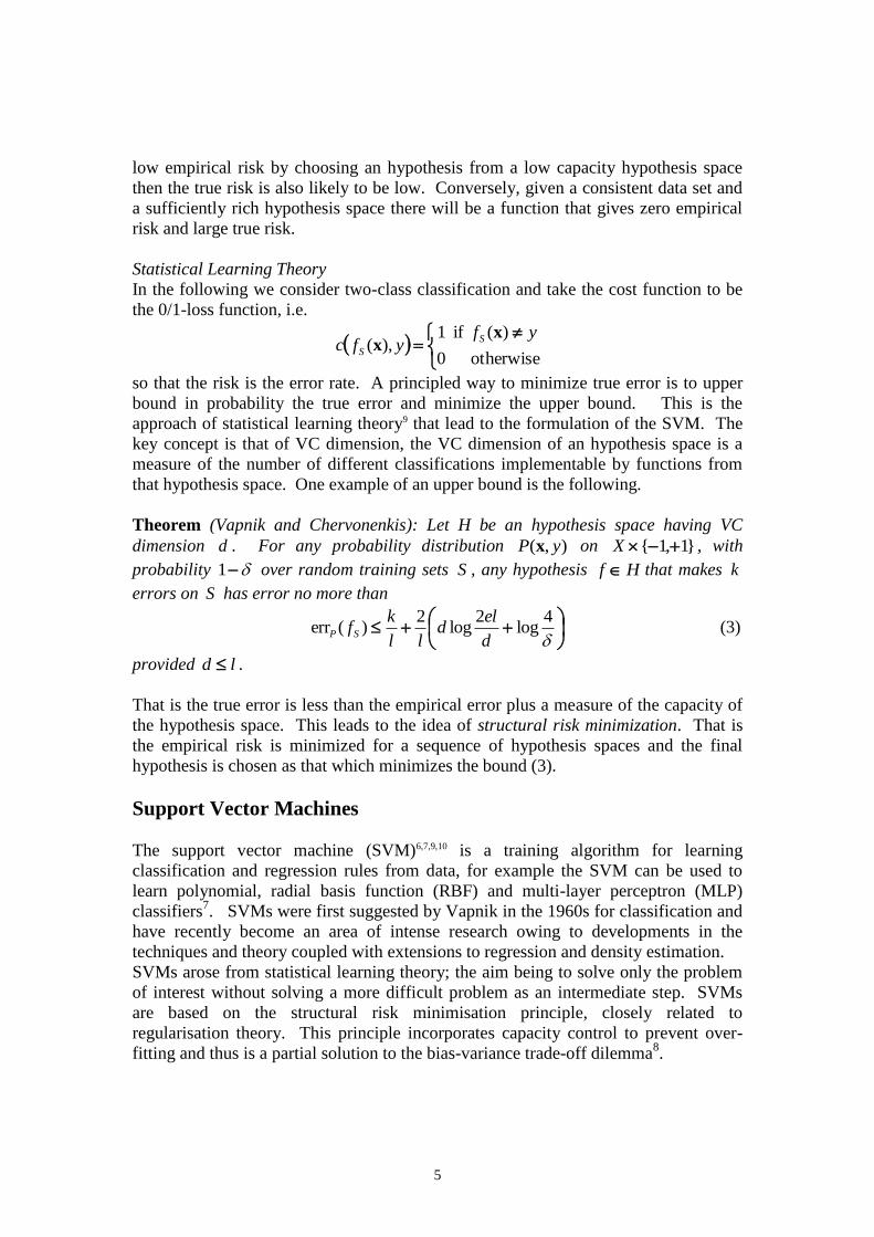
Statistical Learning Theory

In the following we consider two-class classification and take the cost function to be

the 0/1-loss function, i.e.

otherwise0

)( if1),(

yfyfc

S

S

xx

so that the risk is the error rate. A principled way to minimize true error is to upper

bound in probability the true error and minimize the upper bound. This is the

approach of statistical learning theory9 that lead to the formulation of the SVM. The

key concept is that of VC dimension, the VC dimension of an hypothesis space is a

measure of the number of different classifications implementable by functions from

that hypothesis space. One example of an upper bound is the following.

Theorem (Vapnik and Chervonenkis): Let H be an hypothesis space having VC

dimension d . For any probability distribution ),( yP x on }1,1{ X , with

probability 1 over random training sets S , any hypothesis Hf that makes k

errors on S has error no more than

4log

2log

2)(err

d

eld

ll

kfSP (3)

provided ld .

That is the true error is less than the empirical error plus a measure of the capacity of

the hypothesis space. This leads to the idea of structural risk minimization. That is

the empirical risk is minimized for a sequence of hypothesis spaces and the final

hypothesis is chosen as that which minimizes the bound (3).

Support Vector Machines

The support vector machine (SVM)6,7,9,10 is a training algorithm for learning

classification and regression rules from data, for example the SVM can be used to

learn polynomial, radial basis function (RBF) and multi-layer perceptron (MLP)

classifiers7. SVMs were first suggested by Vapnik in the 1960s for classification and

have recently become an area of intense research owing to developments in the

techniques and theory coupled with extensions to regression and density estimation.

SVMs arose from statistical learning theory; the aim being to solve only the problem

of interest without solving a more difficult problem as an intermediate step. SVMs

are based on the structural risk minimisation principle, closely related to

regularisation theory. This principle incorporates capacity control to prevent over-

fitting and thus is a partial solution to the bias-variance trade-off dilemma8.

6

Two key elements in the implementation of SVM are the techniques of mathematical

programming and kernel functions. The parameters are found by solving a quadratic

programming problem with linear equality and inequality constraints; rather than by

solving a non-convex, unconstrained optimisation problem. The flexibility of kernel

functions allows the SVM to search a wide variety of hypothesis spaces.

Here we focus on SVMs for two-class classification, the classes being NP, for

1,1iy respectively. This can easily be extended to k class classification by

constructing k two-class classifiers9. The geometrical interpretation of support

vector classification (SVC) is that the algorithm searches for the optimal separating

surface, i.e. the hyperplane that is, in a sense, equidistant from the two classes10

. This

optimal separating hyperplane has many nice statistical properties9. SVC is outlined

first for the linearly separable case. Kernel functions are then introduced in order to

construct non-linear decision surfaces. Finally, for noisy data, when complete

separation of the two classes may not be desirable, slack variables are introduced to

allow for training errors.

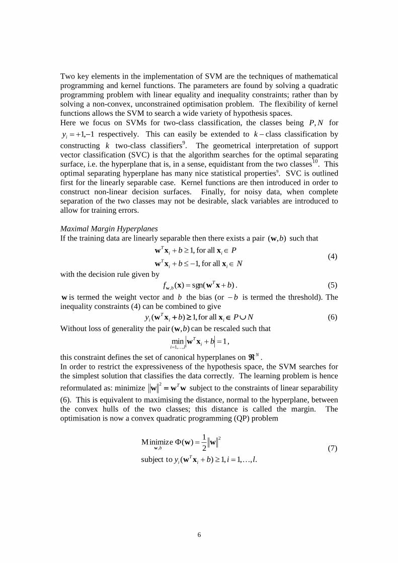
Maximal Margin Hyperplanes

If the training data are linearly separable then there exists a pair ),( bw such that

Nb

Pb

ii

T

ii

T

xxw

xxw

allfor ,1

allfor ,1 (4)

with the decision rule given by

)sgn()(, bf T

b xwxw . (5)

w is termed the weight vector and b the bias (or b is termed the threshold). The

inequality constraints (4) can be combined to give

NPby ii

T

i xxw allfor ,1)( (6)

Without loss of generality the pair ),( bw can be rescaled such that

1min,,1

bi

T

lixw

,

this constraint defines the set of canonical hyperplanes on N .

In order to restrict the expressiveness of the hypothesis space, the SVM searches for

the simplest solution that classifies the data correctly. The learning problem is hence

reformulated as: minimize wwwT

2 subject to the constraints of linear separability

(6). This is equivalent to maximising the distance, normal to the hyperplane, between

the convex hulls of the two classes; this distance is called the margin. The

optimisation is now a convex quadratic programming (QP) problem

.,,1,1)( subject to

2

1)( Minimize

2

,

liby i

T

i

b

xw

www (7)

7

This problem has a global optimum; thus the problem of many local optima in the

case of training e.g. a neural network is avoided. This has the advantage that

parameters in a QP solver will affect only the training time, and not the quality of the

solution. This problem is tractable but in order to proceed to the non-separable and

non-linear cases it is useful to consider the dual problem as outlined below. The

Lagrangian for this problem is

l

i

i

T

ii bybL1

21)(

2

1),,( xwww (8)

where T

l ),,( 1 are the Lagrange multipliers, one for each data point. The

solution to this quadratic programming problem is given by maximising L with

respect to 0 and minimising with respect to b,w . Differentiating with respect to

w and b and setting the derivatives equal to 0 yields

0),,(

1

l

i

iii ybL

xww

w

and

l

i

ii yb

bL

1

0),,(

w. (9)

So that the optimal solution is given by (5) with weight vector

l

i

iii y1

**xw (10).

Substituting (9) and (10) into (8) we can write

l

i

l

j

j

T

ijiji

l

i

i

l

i

i yyF1 11

2

1 2

1

2

1)( xxw (11)

which, written in matrix notation, leads to the following dual problem

0,0 subject to

2

1)( Maximize

y

DIF

T

TT

(12)

where T

lyyy ),,( 1 and D is a symmetric ll matrix with elements

j

T

ijiij yyD xx . Note that the Lagrange multipliers are only non-zero when

1)( by i

T

i xw , vectors for which this is the case are called support vectors since

they lie closest to the separating hyperplane. The optimal weights are given by (10)

and the bias is given by

i

T

iyb xw** (13)

for any support vector ix (although in practice it is safer to average over all support

vectors10). The decision function is then given by

l

i

i

T

ii byf1

**sgn)( xxx . (14)

8

The solution obtained is often sparse since only those ix with non-zero Lagrange

multipliers appear in the solution. This is important when the data to be classified are

very large, as is often the case in practical data mining situations. However, it is

possible that the expansion includes a large proportion of the training data, which

leads to a model that is expensive both to store and to evaluate. Alleviating this

problem is one area of ongoing research in SVMs.

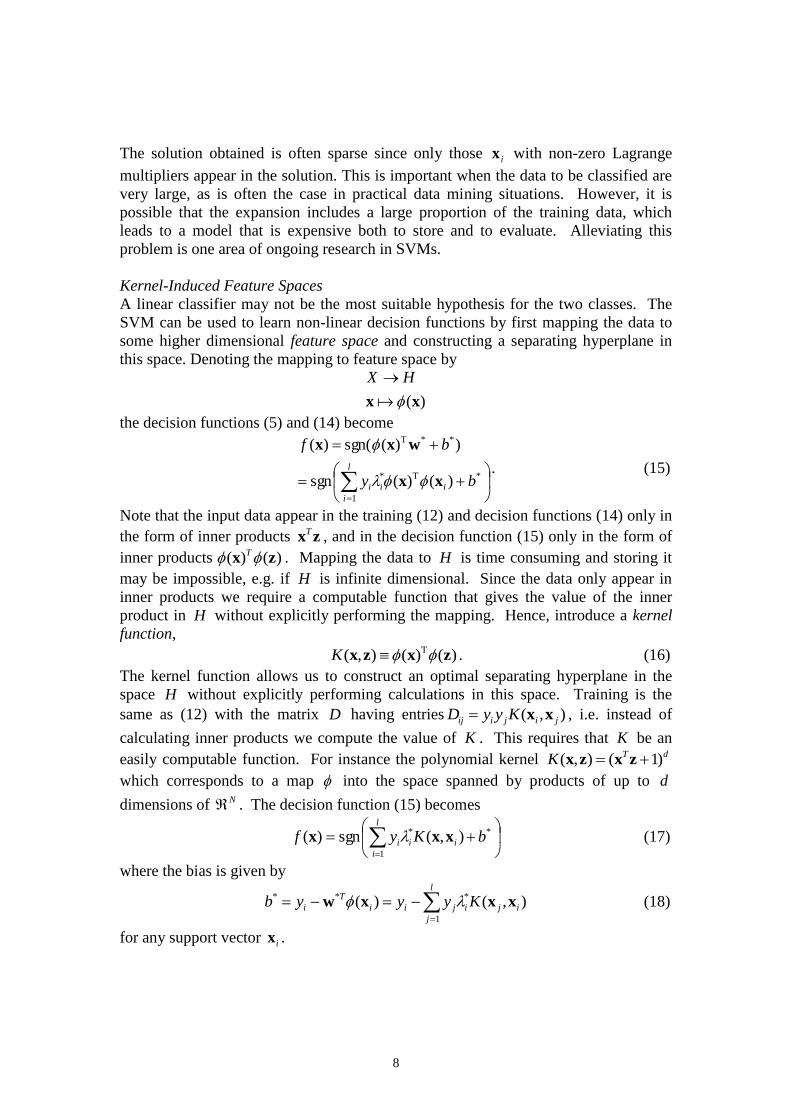
Kernel-Induced Feature Spaces

A linear classifier may not be the most suitable hypothesis for the two classes. The

SVM can be used to learn non-linear decision functions by first mapping the data to

some higher dimensional feature space and constructing a separating hyperplane in

this space. Denoting the mapping to feature space by

)(xx

HX

the decision functions (5) and (14) become

l

i

iii by

bf

1

*T*

**T

)()(sgn

))(sgn()(

xx

wxx

. (15)

Note that the input data appear in the training (12) and decision functions (14) only in

the form of inner products zxT , and in the decision function (15) only in the form of

inner products )()( zx T . Mapping the data to H is time consuming and storing it

may be impossible, e.g. if H is infinite dimensional. Since the data only appear in

inner products we require a computable function that gives the value of the inner

product in H without explicitly performing the mapping. Hence, introduce a kernel

function,

)()(),( Tzxzx K . (16)

The kernel function allows us to construct an optimal separating hyperplane in the

space H without explicitly performing calculations in this space. Training is the

same as (12) with the matrix D having entries ),( jijiij KyyD xx , i.e. instead of

calculating inner products we compute the value of K . This requires that K be an

easily computable function. For instance the polynomial kernel dTK )1(),( zxzx

which corresponds to a map into the space spanned by products of up to d

dimensions of N . The decision function (15) becomes

l

i

iii bKyf1

** ),(sgn)( xxx (17)

where the bias is given by

l

j

ijijii

T

i Kyyyb1

*** ),()( xxxw (18)

for any support vector ix .

9

The only remaining problem is specification of the kernel function, the kernel should

be easy to compute, well-defined and span a sufficiently rich hypothesis space7. A

common approach is to define a positive definite kernel that corresponds to a known

classifier such as a Gaussian RBF, two-layer MLP or polynomial classifier. This is

possible since Mercer’s theorem states that any positive definite kernel corresponds to

an inner product in some feature space. Kernels can also be constructed to incorporate

domain knowledge11

.

This so-called ‘kernel trick’ gives the SVM great flexibility. With a suitable choice of

parameters an SVM can separate any consistent data set (that is, one where points of

distinct classes are not coincident). Usually this flexibility would cause a learner to

overfit the data; i.e. the learner would be able to model the noise in the data as well as

the data-generating process. Overfitting is one of the main problems of data mining

in general and many heuristics have been developed to prevent it, including pruning

decision trees12

, weight linkage and weight decay in neural networks8, and statistical

methods of estimating future error13

. The SVM mostly side-steps the issue by using

regularisation, that is the data are separated with a large margin. The space of

classifiers that separate the data with a large margin has much lower capacity than the

space of all classifiers searched over6. Intuitively, if the data can be classified with

low error by a simple decision surface then we expect it to generalize well to unseen

examples.

Non-Separable Data

So far we have restricted ourselves to the case where the two classes are noise-free.

In the case of noisy data, forcing zero training error will lead to poor generalisation.

This is because the learned classifier is fitting the idiosyncrasies of the noise in the

training data. To take account of the fact that some data points may be misclassified

we introduce a vector of slack variables T

l ),,( 1 that measure the amount of

violation of the constraints (6). The problem can then be written

liby

Cb

iii

T

i

l

i

k

i

,,1,0,1))(( subject to

2

1),,( Minimize

1

2

b,,

xw

www

(19)

where C and k are specified beforehand. C is a regularisation parameter that

controls the trade-off between maximising the margin and minimising the training

error term. If C is too small then insufficient stress will be placed on fitting the

training data. If C is too large then the algorithm will overfit the training data. Due

to the statistical properties of the optimal separating hyperplane, C can be chosen

without the need for a holdout validation set9. If 0k then the second term counts

the number of training errors. In this case the optimisation problem is NP-complete9.

The lowest value for which (19) is tractable is 1k . The value 2k is also used

although this is more sensitive to outliers in the data. If we choose 2k then we are

performing regularized least squares, i.e. the assumption is that the noise in x is

10

normally distributed6. In noisy domains we look for a robust classifier

14 and hence

choose 1k . The Lagrangian for this problem is

l

i

i

l

i

ii

l

i

ii

T

ii

C

bybL

11

1

2]1))(([

2

1),,,,(

xwww

(20)

where T

l ),,( 1 , as before, and T

l ),,( 1 are the Lagrange multipliers

corresponding to the positivity of the slack variables. The solution of this problem is

the saddle point of the Lagrangian given by minimising L with respect to ,w and b ,

and maximising with respect to 0 and 0 . Differentiating with respect to w ,

b and and setting the results equal to zero we obtain

0)(),,,,(

1

l

i

iii ybL

xww

w

,

0),,,,(

1

l

i

ii yb

bL

w, (21)

and

.0),,,,(

ii

i

CbL

w (22)

So that the optimal weights are given by

l

i

iii y1

* )(xw (23)

Substituting (21), (22) and (23) into (20) gives the following dual problem

0,0 subject to

2

1)( Maximize

yC

DIF

T

TT

(24),

where T

lyyy ),,( 1 and D is a symmetric ll matrix with elements

),( jijiij KyyD xx . The decision function implemented is exactly as before in (17).

The bias term *b is given by (18) where ix is a support vector for which Ci 0 .

There is no proof that such a vector exists but empirically this is usually the case. If

all support vectors have C then the solution is said to be unstable, as the global

optimum is not unique. In this case the optimal bias can be calculated by an appeal to

the geometry of the hyperplane15

.

Thus the SVM learns the optimal separating hyperplane in some feature space, subject

to ignoring certain points which become training misclassifications. The learnt

hyperplane is an expansion on a subset of the training data known as the support

vectors. By use of an appropriate kernel function the SVM can learn a wide range of

classifiers including a large set of RBF networks and neural networks. The flexibility

of the kernels does not lead to overfitting since the space of hyperplanes separating

11

the data with large margin has much lower capacity than the space of all

implementable hyperplanes.

Practical Considerations

Much of the present research activity in SVMs is concerned with reducing training

time16,17

, parameter selection18,19

and reducing the size of the model20

. Most existing

algorithms for SVMs scale as )()( 3lOlO in the number of training examples. Most

empirical evaluations of algorithmic scaling tend to focus of linearly separable data

sets with sparse feature representations that are not characteristic of data mining

problems in general. The majority of research in SVMs is focussed on attaining the

global minimum of the QP (24). From a data mining perspective this may not be

necessary. There are a variety of other stopping criteria that could be used and should

be available in a general purpose SVM package for data mining. These include

limiting training time and tracking predicted error. If the predicted error falls below a

pre-specified target, or if it does not appear to be decreasing then one may wish to

terminate the algorithm, as progressing to the global optimum will be unnecessary and

time-consuming. In order to track predicted error one can appeal to statistical

learning theory to provide an upper bound on the expected leave-one-out error21

.

Theorem (Joachims, 2000) The leave-one-out error rate of a stable SVM on a

training set S is bounded by

}1)2(:{)),(( 2

1

\

ii

l

i

iiiS Riyfc x

where iSf \ is the SVM solution when example i is omitted from the training set S and 2R is an upper bound on liK ii ,,1),,( xx .

This quantity can be calculated at very little cost from the current set of Lagrange

multipliers . The leave-one-out error

l

i iiiS yfc1 \ )),(( x is an unbiased estimate of

the true error. It is generally expensive to calculate but due the statistical properties of

the SVM it can be bounded by an easily computable quantity.

Another important point when using SVMs is data reduction. When the data are

noisy the number of non-zero i can be a significant fraction of the data set. This

leads to a large model that is expensive to store and evaluate on future examples. One

way to avoid this is to cluster the data and use the cluster centres as a reduced

representation of the data set. This leads to a more compact model with performance

close to the optimal22

.

The primal formulations (7), (19) lead to the need to enforce the equality constraint

(9), (21) when solving the dual. A simple amendment to the algorithm is to include

the term 2

2

1b in the primal formulations. This removes the need to enforce the

equality constraint as the requirement that the derivative of the Lagrangian with

respect to b is zero now leads to yb T , and the matrix D in (12), (24) has entries

12

given by )1),(( jijiij KyyD xx . The solution to this QP leads to performance

almost identical to the standard formulation on a wide range of real world data sets23

.

Discussion

Related Algorithms

For want of space this section is a brief summary of other applications of the SVM to

data mining problems, further details can be found in the references.

The SVM can be extended to regression estimation6,7,9,10

by introducing an

-insensitive loss function

ppfyfyfyL ))(,0max()(),,(

xxx ,

where }2,1{p . This loss function only counts as errors those predictions that are

more that away from the training data. This loss function allows the concepts of

margin to be carried over to the regression case keeping all of the nice statistical

properties. Support vector regression also results in a QP.

An interesting application of the SVM methodology is to novelty detection24

. The

objective is to find the smallest sphere that contains a given percentage of the data.

This also leads to a QP. The ‘support vectors’ are points lying on the sphere and the

‘training errors’ are outliers, or novelties (depending on your point of view). The

technique can also be generalized to kernel spaces to provide a graded, or

hierarchical, clustering of the data.

SVMs fall into the intersection of two research areas: kernel methods25

, and large

margin classifiers26

. These methods have been applied to feature selection, time

series analysis, reconstruction of a chaotic system, and non-linear principal

components. Further advances in these areas are to be expected in the near future.

SVMs and related methods are also being increasingly applied to real world data

mining, an up-to-date list of such applications can be found at

http://www.clopinet.com/isabelle/Projects/SVM/applist.html.

Summary and Conclusions

The support vector machine has been introduced as a robust tool for many aspects of

data mining including classification, regression and outlier detection. The SVM for

classification has been detailed and some practical considerations mentioned. The

SVM uses statistical learning theory to search for a regularized hypothesis that fits the

available data well without over-fitting. The SVM has very few free parameters, and

these can be optimized using generalisation theory without the need for a separate

validation set during training. The SVM does not fall into the class of ‘just another

algorithm’ as it is based on firm statistical and mathematical foundations concerning

generalisation and optimisation theory. Moreover, it has been shown to outperform

existing techniques on a wide variety of real world problems. SVMs will not solve

all of your problems, but as kernel methods and maximum margin methods are further

improved and taken up by the data mining community they will become an essential

tool in any data miner’s toolkit.

13

Acknowledgements

This research has been undertaken within the INTErSECT Faraday Partnership

managed by Sira Ltd and the National Physical Laboratory, and has been supported

by the Engineering and Physical Sciences Research Council (EPSRC),

GlaxoSmithKline and Sira Ltd.

Robert Burbidge is an associate of the Postgraduate Training Partnership established

between Sira Ltd and University College London. Postgraduate Training Partnerships

are a joint initiative of the Department of Trade and Industry and EPSRC.

References 1 T. Mitchell. Machine Learning. McGraw-Hill International, 1997.

2 R.A. Fisher. The use of multiple measurements in taxonomic problems. Annual

Eugenics, 7 (Part II): 179-188, 1936. 3 D. Harrison and D.L. Rubinfeld. Hedonic prices and the demand for clean air. J.

Environ. Economics and Management, 5:81-102, 1978. 4 F. Rosenblatt. The perceptron: a probabilistic model for information storage and

organization in the brain. Psychological Review, 65:386-408, 1959. 5 R. Duda and P. Hart. Pattern Classification and Scene Analysis. John Wiley &

Sons, 1973. 6 N. Cristianini and J. Shawe-Taylor. An Introduction to Support Vector Machines.

Cambridge University Press, 2000. 7 E. Osuna, R. Freund, and F. Girosi. Support vector machines: training and

applications. AI Memo 1602, MIT, May 1997. 8 C. Bishop. Neural Networks for Pattern Recognition. Clarendon Press, 1995.

9 V. Vapnik. Statistical Learning Theory. John Wiley & Sons, 1998.

10 C.J.C. Burges. A tutorial on support vector machines for pattern recognition. Data

Mining and Knowledge Discovery, 2(2):1-47, 1998. 11

A. Zien, G. Rätsch, S. Mika, B. Schölkopf, C. Lemmen, A. Smola, T. Lengauer,

and K.-R. Müller. Engineering support vector machine kernels that recognize

translation initiation sites. German Conference on Bioinformatics, 1999. 12

L. Breiman, J.H. Friedman, R.A. Olshen, and C.J. Stone. Classification and

Regression Trees, Chapman & Hall, 1984. 13

B.D. Ripley. Pattern Recognition and Neural Networks, Cambridge University

Press, 1996. 14

P. Huber. Robust Statistics, John Wiley & Sons, 1981. 15

C. Burges and D. Crisp. Uniqueness of the SVM solution. In Proceedings of the

Twelfth Conference on Neural Information Processing Systems. S. A. Solla,

T. K. Leen, and K.-R. Müller (Eds.), MIT Press, 1999. 16

T. Joachims. Making large-scale support vector machine learning practical. In

Advances in Kernel Methods: Support Vector Learning. B. Schölkopf, C.J.C. Burges,

and A.J. Smola (Eds.), MIT Press, 1998.

14

17

J.C. Platt. Fast training of support vector machines using sequential minimal

optimization. In Advances in Kernel Methods: Support Vector Learning.

B. Schölkopf, C.J.C. Burges, and A.J. Smola (Eds.), MIT Press, 1998. 18

O. Chapelle and V. Vapnik. Model selection for support vector machines. In

Proceedings of the Twelfth Conference on Neural Information Processing Systems.

S.A. Solla, T. K. Leen, and K.-R. Müller (Eds.), MIT Press, 1999. 19

J.-H. Lee and C.-J. Lin. Automatic model selection for support vector machines.

Available from http://www.csie.ntu.edu.tw/~cjlin/papers.html, 2000. 20

G. Fung, O. L. Mangasarian, and A J. Smola. Minimal Kernel Classifiers. Data

Mining Institute Technical Report 00-08, November 2000. IEEE Transactions on

Pattern Analysis and Machine Intelligence, submitted. 21

T. Joachims. Estimating the generalization performance of a SVM Efficiently. In

Proceedings of the International Conference on Machine Learning. Morgan

Kaufman, 2000. 22

G. Fung and O. L. Mangasarian. Data selection for support vector machine

classifiers. Data Mining Institute Technical Report 00-02, February 2000. In

Proceedings of the Sixth ACM SIGKDD International Conference on Knowledge

Discovery and Data Mining, August 20-23, 2000, Boston, MA, R. Ramakrishnan and

S. Stolfo (Eds.) ACM, NY 2000, 64-70. 23

C.-W. Hsu and C.-J. Lin. A simple decomposition method for support vector

machines. To appear in Machine Learning, 2001. 24

D.M.J. Tax and R.P.W. Duin. Data domain description using support vectors. In

Proceedings of European Symposium on Artificial Neural Networks '99, Brugge,

1999. 25

B. Schölkopf, C.J.C. Burges, and A.J. Smola (Eds.). Advances in Kernel Methods:

Support Vector Learning. MIT Press, 1998. 26

A.J. Smola, P.L. Bartlett, B. Schölkopf, and D. Schuurmans (Eds.). Advances in

Large Margin Classifiers. MIT Press, 2000.