An introduction to ROOT

Andrea Di SimoneUni Freiburg

OutlineOutline

➢ Data analysis

➢ ROOT➢ General concepts

➢ Data representation➢ Histograms➢ Profiles➢ Graphs

➢ Data interpretation➢ Functions➢ Fits

➢ Data input/output➢ Trees

Data AnalysisData Analysis

➢ Aim is to derive physical meaning from input numbers

➢ Need tools to visualize data, manipulate it, perform statistical analysis

➢ A set of data structures are common to most scientific analysis➢ Histograms, graphs, profiles

➢ Specific analyses may need special structures➢ Extensibility

➢ Must be efficient and stable (computationally) for analysis of large input data sets

ROOTROOT

➢ A Toolkit (not a program) to perform data analysis

➢ C++ as implementation language➢ A huge set of classes, covering all aspects of analysis,

from representation to interpretation to I/O

➢ User writes his/her own program➢ In C++, usually

➢ A C++ interpreter (CINT) is provided for interactive analysis➢ It executes your C++ commands while you type them

➢ Provides some shortcuts and simplifications wrt the “official” C++ syntax

General conceptsGeneral concepts

➢ You pass to the interpreter your commands➢ You may not appreciate it, but they all are C++ statements

➢ You create instance of classes, call methods of classes and so on

➢ All names of classes start with capital T➢ TH1F, TGraph, TNtuple

➢ All methods start with capital letter, capitalization repeated at each new word➢ TH1F::Draw() TH1F::GetBinContents(...)

➢ Some “global” instances defined automatically by the interpreter when you launch it. Their names start with lower case g➢ gROOT, gPad, gDirectory

General concepts (2)General concepts (2)

➢ Most of the objects you will use inherit from TObject class➢ It means that they are specializations of TObject

➢ In the same way as a dog is a specialization of a mammal

➢ Some high level manipulation of objects is done automatically for you by the ROOT kernel, and most of the times this is done using TObject➢ Even if you create a histogram, at a higher level it is

treated just as a TObject

➢ Keep it in mind when dealing with the kernel (see the following slides)

General concepts (3)General concepts (3)

➢ Most of the objects you will deal with, have a Title and a Name➢ Take care to set them to meaningful values

➢ It's done by using SetName and SetTitle methods

➢ For plottable objects (graphs, histograms, profiles), the title is the one who will appear on the actual plot

➢ Names have a role on the internal memory management of ROOT, so try not to duplicate them, in particular for “important” objects➢ It's not forbidden, but I strongly suggest not to do it

General Concepts (4)General Concepts (4)

➢ You can run your analysis interactively, line by line➢ Good for fast debugging

➢ You can write your C++ program using ROOT classes, compile it and run ➢ Good for massive production and analysis of large datasets

➢ You can also save many ROOT commands in a macro file and pass it to CINT as a whole➢ A nice compromise between flexibility and robustness

➢ Remember: CINT is an interpreter➢ In general, your code will go considerably slower than a

“real” compiled application➢ There are a couple of tricks to improve this, but we will not cover

them here

General Concepts (5)General Concepts (5)

➢ ROOT has a very powerful GUI

➢ Improving at every new release

➢ Most of the things I'll show you here can be done from the GUI, without using the command line

➢ However, the command line is essential when running scripts➢ As a general suggestion, use the GUI as a shortcut,

but be sure you can live without it

gROOTgROOT

➢ Instance of the TROOT object

➢ Created by CINT when starting up

➢ It's the access point to the ROOT kernel➢ Beyond the scope of this introductory course

➢ Just remember this one: gROOT.SetStyle(“Plain”)

➢ It also keeps track of the objects you create, allowing you to retrieve them later on➢ gROOT.FindObjectByName(“MyLostObject”)

➢ Beware: this will return a Tobject*➢ myLostHisto=(TH1F*)gROOT.FindObjectByName(“MyLostHistoName”)

Data representationData representation

HistogramsHistograms

➢ How often does my variable have a certain value?

➢ A histogram is defined by giving the number of bins and the range of values➢ TH1F * histo= new TH1F(“testName”, “testTitle”,1000,0,1000)

➢ You can fill a number into the hitogram by calling TH1F::Fill()➢ histo.Fill(10) will increase by one

the counts in the bin “covering”

the value 10

➢ histo.Fill(10,2) will increase by

2 the counts in the bin “covering”

the value 10 (example of event weight)

➢ The histogram “knows” its two axes➢ To access them, for example to change the axis title, use the

methods GetXaxis() and GetYaxis()

Histograms (2)Histograms (2)➢ You can do many things with histograms

➢ Rebin them (i.e. merge together adjacent bins)➢ TH1F::Rebin(nBinsToMerge)

➢ Sum two histograms➢ TH1F histo1, histo2➢ TH1F total=histo1+histo2

➢ Multiply and divide (by an integer or by another histogram)

➢ Set maximum and minimum of y axis➢ TH1F::SetMaximum TH1F::SetMinimum

➢ Set colors➢ TH1F::SetFillColor TH1F::SetLineColor

➢ You can draw 2 histos on the same plot using the “same” drawing option➢ myFirstHisto.Draw()➢ mySecondHisto.Draw(“same”)

➢ I have 2 variables. How often does my variable 2 have a certain value once we fix the value of variable 1?

➢ Creation is similar to 1D histograms. Obviously, you need to give binning and range information TWICE➢ TH2F * histo= new TH1F(“testName”,

“testTitle”,1000,0,1000, 2000,0,2000)

➢ Operations similar to 1D histograms

➢ You can have nice 3D plots using special options in the Draw method➢ my2Dhisto.Draw(“lego”)

2D Histograms2D Histograms

➢ At any time, you can reset the contents of a histogram (both 1D and 2D), by using TH*F::Reset()

➢ Note that minimum and maximum settings act on the “third” axis, not on the ones containing your variables

➢ The Fill method of course has TWO arguments, plus the optional weight

2D Histograms: graphic options2D Histograms: graphic options➢ Two very useful options:

➢ myHisto.Draw(“box”): the area is divided in boxes with the same dimensions as the bins. Inside each box another box is drawn, its area proportional to the bin contents➢ Larger box means more entries in the bin

➢ myHisto.Draw(“lego”): the third axis is drawn explicitly, and a lego plot is shown➢ You can rotate it with the mouse

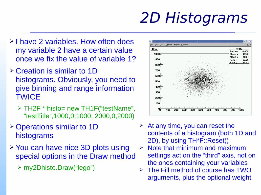
Graphic Options (2)Graphic Options (2)

➢ “col”: will print a scatter plot, with colors corresponding to bin entries

➢ “surf”: similar to lego, but a surface is drawn instead of the 3D bins

GraphsGraphs➢ Graphs plot on a canvas 2-D data

➢ Needed when you want to plot (x,y) pairs

➢ Several possible constructors➢ Example:

➢ TGraph myGr➢ myGR.SetPoint(0,0,0)➢ myGR.SetPoint(1,1,0)➢ myGR.SetPoint(2,4,4)➢ myGR.SetPoint(3,6,9)

➢ Once you filled it with points, you can draw it with the Draw method

➢ Several Draw options, see following slide

Graphic optionsGraphic options

➢ For example, you decide whether you want the axes the points, a line

➢ Note: if you don't specify anything, you'll have a blank plot

“apl”

“ap”“al”

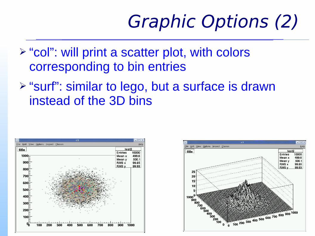
Graphs with errorsGraphs with errors

➢ The corresponding class is TGraphErrors

➢ Similar interface as plain TGraphs

➢ Methods for error setting/retrieving added➢ TGraphErrors::SetPointError(nPoint, errX, errY)

➢ Same graphic options as normal graphs

➢ Another class with asymmetric errors is available too: TGraphAsymmErrors

ProfilesProfiles

➢ Very powerful for representing 2D data in 1D only

➢ Think of it as a histogram➢ TProfile myPr(“name”, “title”, 100,0,100)

➢ The Fill method has a different signature:➢ myPR.Fill(x,y,weight)

➢ For each bin in x, the profile will show the average of the y values which were filled into that bin

➢ You can draw with errors➢ In this case they will represent the standard deviation

of the values

Profiles: exampleProfiles: example

➢ myPR=TProfile(“title”,”name”,100,0,100)

➢ for(int k=0;k<1000;k++){➢ myPR.Fill(gRandom.Uniform(0,100), gRandom.Gaus(500,100))

➢ }

➢ Example of creation and filling of a profile

➢ Note the use of gRandom for random number creation

Data interpetationData interpetation

FunctionsFunctions

➢ TF1 is the class representing a 1D function➢ Definition is straightforward. You need a name, a

formula, and the range of validity➢ TF1 myFunc(“name”,”2*x*x+20*sin(x)”,0,10)

➢ Draw() will draw the function

➢ Eval(x) will return the value of the function at point x

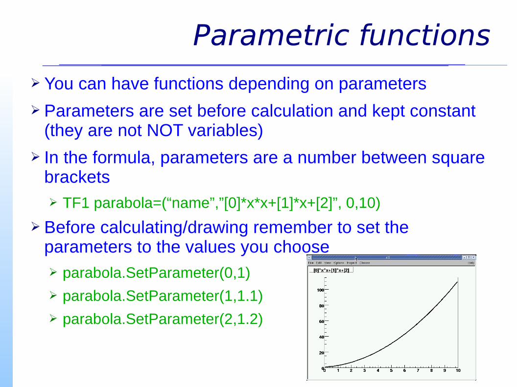
Parametric functionsParametric functions

➢ You can have functions depending on parameters

➢ Parameters are set before calculation and kept constant (they are not NOT variables)

➢ In the formula, parameters are a number between square brackets➢ TF1 parabola=(“name”,”[0]*x*x+[1]*x+[2]”, 0,10)

➢ Before calculating/drawing remember to set the parameters to the values you choose➢ parabola.SetParameter(0,1)

➢ parabola.SetParameter(1,1.1)

➢ parabola.SetParameter(2,1.2)

FitsFits

➢ Parametric functions are crucial when doing fits

➢ You can leave some of the parameters free to float

➢ Their value will be decided trying to maximize the agreement of your function with a set of data you provide➢ Histogram, graph, profile

➢ This is called fitting the data with the function

➢ To do a fit, you need➢ Data

➢ A parametric function

Fits (2)Fits (2)

➢ If you want to use a “simple” function, you can profit from a predefined one➢ Gaussian, polynomial, exponential...

➢ For more complicated cases, you'll have to write the function yourself➢ When using a custom function, remember to set the parameters

to some sensible value before fitting, to help convergence

➢ myHisto.Fit(“gaus”)

➢ myPR.Fit(“pol0”)

Data input/outputData input/output

TFileTFile

➢ Several ways to manage I/O to/from ROOT➢ Far beyond the scope of this introduction

➢ Will focus here on a few recipes for easy and common applications

➢ Let's start from the output➢ You have created several histos, functions, profiles, and

want to save them so that you don' have to restart from scratch next time

➢ ROOT has a native file format, where a user can save (almost) any ROOT object➢ ROOT file format is managed by the class TFile, to be

used both for input and output files

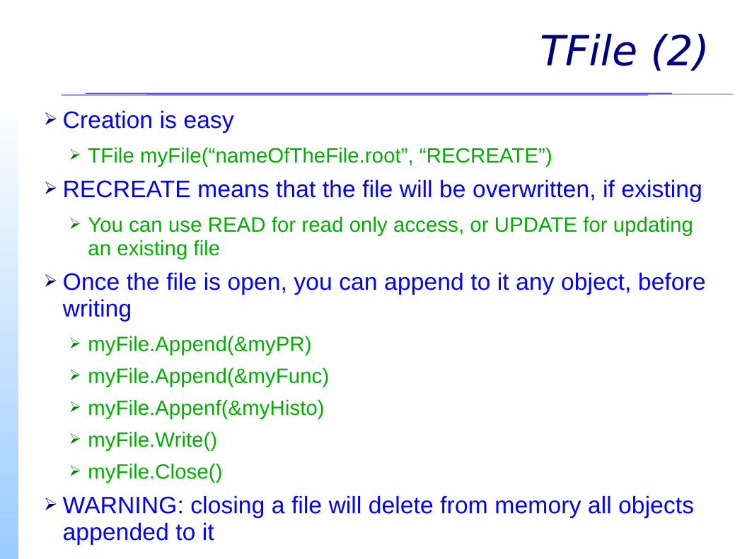
TFile (2)TFile (2)➢ Creation is easy

➢ TFile myFile(“nameOfTheFile.root”, “RECREATE”)

➢ RECREATE means that the file will be overwritten, if existing➢ You can use READ for read only access, or UPDATE for updating

an existing file

➢ Once the file is open, you can append to it any object, before writing➢ myFile.Append(&myPR)

➢ myFile.Append(&myFunc)

➢ myFile.Appenf(&myHisto)

➢ myFile.Write()

➢ myFile.Close()

➢ WARNING: closing a file will delete from memory all objects appended to it

TFile (3)TFile (3)

➢ Reading back is easy too➢ TFile f(“myFile.root”,”READ”)

➢ f.ls()

➢ myHisto=(TH1F*)f.Get(“test”)

➢ myHisto.Draw()

TTreesTTrees

➢ Apart from “high level” analysis objects, one may want to store to file (or read from it) also raw data➢ A table, for example

➢ Actually, ROOT provides much more, by means of a complex data structure called Tree➢ The corresponding class is, of course, TTree

➢ You can put into a tree virtually any object no matter how complicated

➢ And store the TTree to a TFile

➢ Trees are very powerful, but we will focus here only on a special type of tree➢ It is a plain table of floating-point numbers

➢ What one typically calls a ntuple

➢ The corresponding class is TNtuple

TNtupleTNtuple

➢ TNtuples are TTrees of numbers with a simple table-like structure

➢ For its creation, you need a name and a list of variables (i.e. the name of the columns)➢ TNtuple myNt(“ntuple”,”ntuple”, ”x1:x2:x3:x4”)

➢ myNt will be a table with 4 columns➢ You can use any string as column name➢ Just be careful not to use twice the same name in the same ntuple

➢ Once the ntuple is defined, you can for example fill it with the contents of a file➢ myNt.ReadFile(“asciiFile.dat”)

TNtupleTNtuple

➢ Now the ntuple has data. You can see the distribution of any variable by using the Draw method of the ntuple➢ myNt.Draw(“x1”)

➢ myNt.Draw(“x2”)

➢ myNt.Draw(“(x2+x3)/x1”)

➢ A very powerful feature are conditional plots➢ You can draw a certain variable (or combination of

variables) only if another variable (or combination) satisfies a condition

➢ The second argument of Draw is the condition➢ myNt.Draw(“x1”,”x2>0”)➢ myNt.Draw(“sin(x1/2.)”,”exp(x3)==x4”)

NTuple DrawingNTuple Drawing

➢ You can also make 2D plots of course➢ myNt.Draw(“x1:x2”)

➢ And use formulas and selections➢ myNt.Draw(“x1:sin(x2)”,”exp(x4)>2”)

➢ The third argument of Draw is graphic option➢ The most used is “same” which will draw the distribution

on the currently selected plot

➢ By default, TNtuple::Draw will create a new histogram called htemp and fill it with the data passing the selection

TNtuple Drawing (2)TNtuple Drawing (2)

➢ The binning and range of htemp are chosen automatically by ROOT by guessing them from the data itself

➢ You may not be satisfied with ROOT's guess➢ Typical error is that you have integers but ROOT fails to

understand it

➢ Fortunately, when calling Draw, you can specify the name and format of the histogram➢ myNt.Draw(“x1>>h1(10,0,10)”,”selection”)

➢ This will create a histo called h1, with 10 bins between 0 and 10, and fill it with the selected entries

➢ You can do the same with 2D plots, just adding the relevant parameters