Embed Size (px)
Citation preview
An introduction to R
Martin Morgan (mailto:[email protected])Computational Biology Shared ResourceFred Hutchinson Cancer Research Center
Seattle, WA, USA
11 September, 2008
Contents
1 Introduction 11.1 About the Computational Biology Shared Resource . . . . . . . . 21.2 Installing R . . . . . . . . . . . . . . . . . . . . . . . . . . . . . . 21.3 Exercises: a very first R session . . . . . . . . . . . . . . . . . . . 3
2 A first work flow 42.1 Data input . . . . . . . . . . . . . . . . . . . . . . . . . . . . . . 42.2 Object exploration and manipulation . . . . . . . . . . . . . . . . 52.3 Visualization . . . . . . . . . . . . . . . . . . . . . . . . . . . . . 82.4 A little statistics . . . . . . . . . . . . . . . . . . . . . . . . . . . 92.5 Ending the session . . . . . . . . . . . . . . . . . . . . . . . . . . 112.6 Exercises . . . . . . . . . . . . . . . . . . . . . . . . . . . . . . . 12
3 The R programming language 153.1 Basic data types . . . . . . . . . . . . . . . . . . . . . . . . . . . 153.2 Subsetting . . . . . . . . . . . . . . . . . . . . . . . . . . . . . . . 193.3 Useful programming operations . . . . . . . . . . . . . . . . . . . 223.4 Exercises . . . . . . . . . . . . . . . . . . . . . . . . . . . . . . . 24
4 Power tips 27
1 Introduction
This document introduces R. It starts with the assumption that the user is newto R, and concludes with the hope that the user is comfortable doing basic datamanipulation and analysis, and is equiped with the tools for discovering thepower and diversity of R for statistical programing.
This section describes the Computational Biology Shared Resource, and thesteps required to install and use R for the first time. The next section walks
1
through a simple work flow reading in data, exploring it, and performing linearregression (in the body of the text) or principle components analysis (in oneof the exercises). The third section introduces R as a programming environ-ment. The document concludes with a few ‘power tips’ that might lead to moreproductive use of R.
The initial sections are pedantic, but subsequent sections assume increasingfamiliarity with R’s help system and the way R ‘works’; in these later sectionsfunctions are used without explict discussion of what they are doing.
1.1 About the Computational Biology Shared Resource
The Computational Biology Shared Resource is a small (2 member!) servicegroup within Computational Biology. We take on a diversity of roles providingcenter-wide assistance related to microarray data analysis, high throughput se-quencing analysis and tool development, and training in software (especially Rand BioConductor) use. We’ll engage in ‘two-week’ projects on an ad hoc and probono basis, and take larger stakes in projects when resources and opportunitiesfor involvement permit.
1.2 Installing R
We will install R from a thumb drive, to avoid overwhelming the network. Nor-mally, though, R can be installed from the internet; one can also use R on PHSservers. The starting point for access is http://cran.r-project.org and alocal mirror of the core of the repository is at http://cran.fhcrc.org (theacronym CRAN stands for the Comprehensive R Archive Network). The R website and local mirror contain pre-compiled binaries with standard installers forMacOS and Windows operating systems, and a number of linux distributions;third party installations using a variety of Linux package managers are alsoavailable.
R consists of a core application, required and recommended packages, andon some operating systems a graphical user interface. The core application iswritten primarily in C, released under the GPL, and the source code is read-ily available (using SVN). Required and recommended packages implement keyfunctionality (e.g., base contains system and other core functionality, stats con-tains functionality for standard descriptive statistics, probability distributions,random number generators, parametric and non-parametric tests, linear models,time series, factor analysis, and the like).
Interaction with R is through a command-line style interface. The user ispresented with a prompt >, types symbol names or expressions, and presses thecarriage return to submit the symbols to the R parser and evaluator. R respondswith numerical or graphical output. Graphical user interfaces available as partof the basic R installation generally integrate the command-line style interface,graphical output, and help systems; they do not provide a ‘point-and-click’solution (other R packages such as Rcmdr attempt this, usually by presenting asubset of R’s overall functionality).
2
A particular strength of R is that functionality provided in the basic instal-lation is augmented by packages contributed by the user community. There arewell over 1000 user-contributed packages. Package quality can be excellent, im-plementing very sophisticated functionality and cutting-edge research method-ologies. CRAN provides a comprehensive registry of packages, including ‘views’that attempt to group some packages by functionality. Additional projects suchas BioConductor (focussing on analysis of high-throughput biological data, withover 250 packages) represent additional resources.
The R web site contains references to books on R,
1.3 Exercises: a very first R session
Exercise 1Copy the OS-specific folder hierarchy from the memory stick to a convenientlocation on your computer. The following assumes that you copied the hierarchyto a folder named RIntro (it avoids confusion in R to use / for the file pathseparator on Windows).
Exercise 2Install R.
1. Windows and Mac: double click on the installer and follow directions.
2. Linux: consult with tutorial assistants.
Normally, R can be installed from http://cran.fhcrc.org .
Exercise 3Check installation / a first R session.
1. Start R (e.g., double-click on the appropriate icon, or select from the ‘start’menu.
2. Enter the text that appears after the > and confirm that you are using Rversion 2.8.0 Under development (unstable) :
> sessionInfo()
R version 2.8.0 Under development (unstable) (2008-08-29 r46457)
x86_64-unknown-linux-gnu
locale:
LC_CTYPE=en_US.UTF-8;LC_NUMERIC=C;LC_TIME=en_US.UTF-8;LC_COLLATE=en_US.UTF-8;LC_MONETARY=C;LC_MESSAGES=en_US.UTF-8;LC_PAPER=en_US.UTF-8;LC_NAME=C;LC_ADDRESS=C;LC_TELEPHONE=C;LC_MEASUREMENT=en_US.UTF-8;LC_IDENTIFICATION=C
attached base packages:
[1] stats graphics utils datasets grDevices methods
[7] base
3. Find help about the functions provided by a library with the command
3
> library(help = stats)
4. Find help about a function, e.g., fivenum with the command
> `?`(fivenum)
5. Load a special purpose library (in this case, for more advanced plotting)
> library(lattice)
End the R session (select n when prompted to save the session).
> q()
2 A first work flow
2.1 Data input
Start R, and navigate so that files can be easily read. For example,
> setwd("~/sharedrsrc/presentations/RIntro")
Since \ is used to ‘escape’ characters in R, it is best to use / for the pathseparator, even on Windows. To confirm that you’ve arrived at the intendeddirectory, execute the list.files function
> list.files()[1] "extdata"
list.files is a fairly typical function. View its help page with the command?list.files. The usage section indicates how the function can be invoked.There are 6 arguments, all of which are named and have a default value (e.g., theargument named path has default value "."). Above, we specified no arguments,so R used default values for each. On the other hand, we might have written
> list.files("extdata", full.names = TRUE)
This illustrates two features of function invocation: unnamed arguments arematched by position (i.e., R assigns extdata to path), named arguments arematched exactly, regardless of position (i.e., full.names is assigned TRUE).
The directory extdata contains a ‘comma-separated value’ file, a formatexported by many spreadsheets. The file contains three columns of data. Thefirst is the row number. The second and third are plant weight, and a characterstring representing whether the weights in the same row are from a ‘control’or ‘treatment’ group. Our file has a header row, containing the names forthe columns, and the row names are in column 1. R has several functionsto read in text files. Here we use read.csv which, as its name suggests, isspecialized for reading comma-separated value files. Our file has a header row,so we indicate this by setting the argument header to the logical value TRUE.We use the row.names function argument to indicate the column containing
4
rows. To discover these arguments and their interpretation, we might have used?read.csv to obtain the help page, or, when more confident of the function,args(read.csv) to be reminded of the available arguments. We want to readthe contents of the file in to R, and to assign the result to a variable that wecan reference later. We’ll call the variable weights, and read the data in with
> weights <- read.csv("extdata/weights.csv", header = TRUE,
+ row.names = 1)
R automatically adds the ’+’ sign at the beginning of a line when it continuesan incomplete command. You don’t need to enter it.
2.2 Object exploration and manipulation
We can now manipulate weights to find out about it’s content. R has a numberof different classes of objects, including user-defined classes. We can find outwhat class weights is
> class(weights)
[1] "data.frame"
Ah, weights is a data.frame. A look at ?data.frame might be good in thelong term. For now, a data.frame is a matrix-like object where all elements ina row are of the same type, but columns can have different type. We can peekat the top of our weights, and summarize its content:
> head(weights)
Weight Group1 4.17 Ctl2 5.58 Ctl3 5.18 Ctl4 6.11 Ctl5 4.50 Ctl6 4.61 Ctl
> dim(weights)
[1] 20 2
The display from head is a useful confirmation that we have read our data incorrectly: there are row names (integer values) followed by two columns of data.dim can be used to determine the dimensions of array-like objects; here we seethat there are 20 rows and 2 columns.
The function summary provides a quick summary of each column of the dataframe.
> summary(weights)
5
Weight GroupMin. :3.590 Ctl:101st Qu.:4.388 Trt:10Median :4.750Mean :4.8463rd Qu.:5.218Max. :6.110
The Weight column contains numerical values, and the summary is appropriatefor this type of data: an indicate of the minimum, first, median, and thirdquartiles, maximum, and mean of the 20 observations in the column. On theother hand, the summary for Group is different: it indicates that there are 10entries labeled Ctl, and an equal number labeled Trt.
It turns out that read.csv has read the two columns of data in as differentclasses. We can determine the class of each column by selecting the column andusing class on the result. There are two ways to select a column of a dataframe, using $ or [[ Thus:
> class(weights$Weight)
[1] "numeric"
> class(weights[["Weight"]])
[1] "numeric"
The Weight column contains numeric data. The numeric data type repre-sents real numbers. Other common data numerical types include integer andcomplex.
Let’s look at the column Weight in all its detail
> weights[["Weight"]]
[1] 4.17 5.58 5.18 6.11 4.50 4.61 5.17 4.53 5.33 5.14 4.81 4.17[13] 4.41 3.59 5.87 3.83 6.03 4.89 4.32 4.69
The display is of numeric values 4.17, 5.58, etc. For convenience, the index ofthe numeric value is printed at the start of each line, e.g., [1] indicates the firstelement.
The column Weights is an example of a vector. All atomic (the meaning of‘atomic’ will become apparent later) objects in R are vectors. Most R operationsact on vectors. For instance,
> log(1 + weights[["Weight"]])
[1] 1.642873 1.884035 1.821318 1.961502 1.704748 1.724551[7] 1.819699 1.710188 1.845300 1.814825 1.759581 1.642873[13] 1.688249 1.523880 1.927164 1.574846 1.950187 1.773256[19] 1.671473 1.738710
6
adds 1 to each element of Weight, and then takes the natural logarithm of eachvalue. This will be discussed further below.
Returning to our exploration of the weights data frame, the Group columncan be accessed and its class determined in the same fashion as Weights:
> weights[["Group"]]
[1] Ctl Ctl Ctl Ctl Ctl Ctl Ctl Ctl Ctl Ctl Trt Trt Trt Trt Trt[16] Trt Trt Trt Trt TrtLevels: Ctl Trt
> class(weights[["Group"]])
[1] "factor"
R recognized the column of character values in the input file, and interpretedthem as factors in the statistical sense. The value of Group is again a vector,but this time a vector of factor levels. There are two different levels of the Groupfactor:
> levels(weights[["Group"]])
[1] "Ctl" "Trt"
These levels are unordered; R also understands ordered factors, and can treatcharacter sequences as just strings without statistical meaning; the stringsAs-Factors and colClasses arguments to read.csv influence how data types areread in to R. A factor is not usefully summarized by concepts such as minimumor median, so summary provides a different description: a tabulation of the num-ber of observations of each level. A more direct way of obtaining the counts iswith the table function:
> table(weights[["Group"]])
Ctl Trt10 10
One often wants to operate on (e.g., determine the class of) columns of adata frame (or rows or columns of a matrix). R offers a number of apply-likefunctions that make it convenient to perform the same operation repeatedly.For example, we can ‘apply’ the class function to each column of weights,and simplify the result to a vector of characters
> sapply(weights, class)
Weight Group"numeric" "factor"
A final useful tool for exploring R objects is str, which reveals the internalstructure of the object.
7
> str(weights)
'data.frame': 20 obs. of 2 variables:$ Weight: num 4.17 5.58 5.18 6.11 4.5 4.61 5.17 4.53 5.33 5.14 ...$ Group : Factor w/ 2 levels "Ctl","Trt": 1 1 1 1 1 1 1 1 1 1 ...
We see in the result of this function all of the information we have discoveredalready, but in a single place and compactly represented: weights is a dataframe with 20 observations of 2 variables. The first variable, Weights, is anumeric (‘num’) vector the first several values of which are presented, and soon. Aspects of the presentation are cryptic at first (e.g., why are the entriesfor Group given as integers?) but are informative as R becomes more familiar(factor objects are encoded as integers indexing the corresponding level; thismakes important operations on factors compact and efficient).
2.3 Visualization
Complex data objects, especially relations between variables, are often bestexplored through visualization. One way to visualize our data is with the plotfunction, providing ‘x’ and ‘y’ variables as arguments, for instance
> plot(weights[["Group"]], weights[["Weight"]])
Let’s take two steps that are more complicated than this. First, we add a packageto the library of packages available in the current session of R. A package is acollection of R functions and other objects that augment built-in functionality.R starts with a list of packages already loaded. We’ll add the lattice package tothis list, with the following command:
> library(lattice)
We can see the set of packages that R searches for functions and other objectswith
> search()
[1] ".GlobalEnv" "package:lattice" "package:stats"[4] "package:graphics" "package:utils" "package:datasets"[7] "package:grDevices" "package:methods" "Autoloads"[10] "package:base"
When the user requests an object, e.g., by invoking a function or attempting todisplay the contents of a data frame, R searches first in the ‘global environment’,which is where user objects like weights get created by default. If the objectis not found in the global environment, R continues to search loaded packages,in the order specified by search(), until the object is found. For instance, thefunction class is found in the base package.
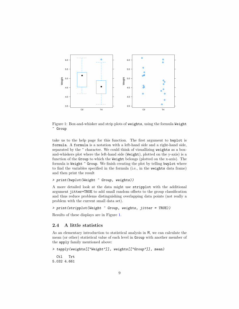
We will use bwplot from lattice to visualize our data; ‘bw’ is an abbreviationof box-and-whiskers; loading lattice loads associated help files, so ?bwplot would
8
Wei
ght
3.5
4.0
4.5
5.0
5.5
6.0
Ctl Trt
●
●
●
Wei
ght
3.5
4.0
4.5
5.0
5.5
6.0
Ctl Trt
●
●
●
●
●
●
●
●
●
●
●
●
●
●
●
●
●
●
●
●
Figure 1: Box-and-whisker and strip plots of weights, using the formula Weight~ Group
take us to the help page for this function. The first argument to bwplot isformula. A formula is a notation with a left-hand side and a right-hand side,separated by the ~ character. We could think of visuallizing weights as a box-and-whiskers plot where the left-hand side (Weight), plotted on the y-axis) is afunction of the Group to which the Weight belongs (plotted on the x-axis). Theformula is Weight ~ Group. We finish creating the plot by telling bwplot whereto find the variables specified in the formula (i.e., in the weights data frame)and then print the result
> print(bwplot(Weight ~ Group, weights))
A more detailed look at the data might use stripplot with the additionalargument jitter=TRUE to add small random offsets to the group classificationand thus reduce problems distinguishing overlapping data points (not really aproblem with the current small data set).
> print(stripplot(Weight ~ Group, weights, jitter = TRUE))
Results of these displays are in Figure 1.
2.4 A little statistics
As an elementary introduction to statistical analysis in R, we can calculate themean (or other) statistical value of each level in Group with another member ofthe apply family mentioned above:
> tapply(weights[["Weight"]], weights[["Group"]], mean)
Ctl Trt5.032 4.661
9
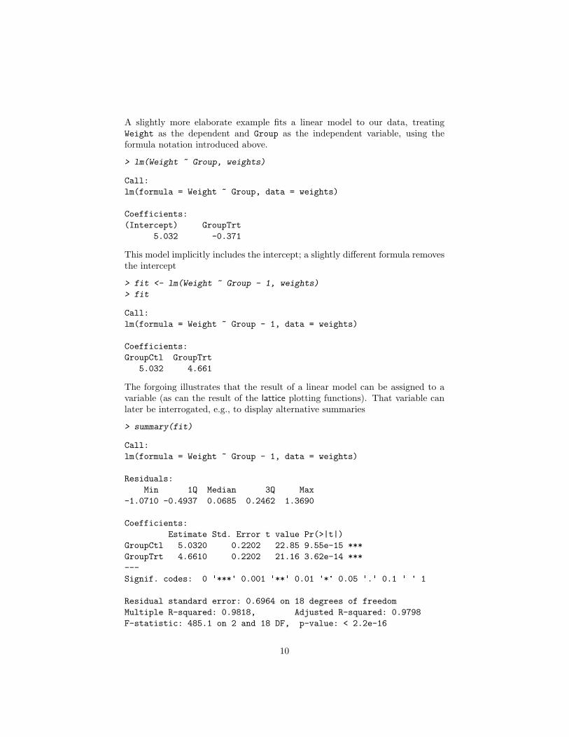
A slightly more elaborate example fits a linear model to our data, treatingWeight as the dependent and Group as the independent variable, using theformula notation introduced above.
> lm(Weight ~ Group, weights)
Call:lm(formula = Weight ~ Group, data = weights)
Coefficients:(Intercept) GroupTrt
5.032 -0.371
This model implicitly includes the intercept; a slightly different formula removesthe intercept
> fit <- lm(Weight ~ Group - 1, weights)
> fit
Call:lm(formula = Weight ~ Group - 1, data = weights)
Coefficients:GroupCtl GroupTrt
5.032 4.661
The forgoing illustrates that the result of a linear model can be assigned to avariable (as can the result of the lattice plotting functions). That variable canlater be interrogated, e.g., to display alternative summaries
> summary(fit)
Call:lm(formula = Weight ~ Group - 1, data = weights)
Residuals:Min 1Q Median 3Q Max
-1.0710 -0.4937 0.0685 0.2462 1.3690
Coefficients:Estimate Std. Error t value Pr(>|t|)
GroupCtl 5.0320 0.2202 22.85 9.55e-15 ***GroupTrt 4.6610 0.2202 21.16 3.62e-14 ***---Signif. codes: 0 '***' 0.001 '**' 0.01 '*' 0.05 '.' 0.1 ' ' 1
Residual standard error: 0.6964 on 18 degrees of freedomMultiple R-squared: 0.9818, Adjusted R-squared: 0.9798F-statistic: 485.1 on 2 and 18 DF, p-value: < 2.2e-16
10
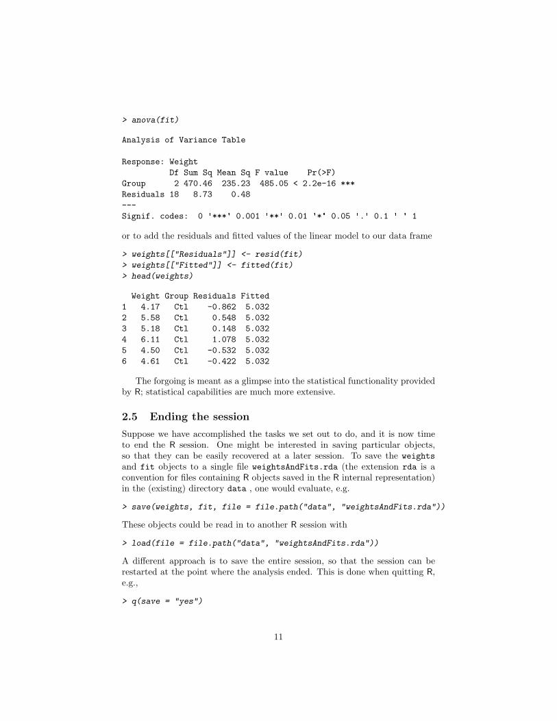
> anova(fit)
Analysis of Variance Table
Response: WeightDf Sum Sq Mean Sq F value Pr(>F)
Group 2 470.46 235.23 485.05 < 2.2e-16 ***Residuals 18 8.73 0.48---Signif. codes: 0 '***' 0.001 '**' 0.01 '*' 0.05 '.' 0.1 ' ' 1
or to add the residuals and fitted values of the linear model to our data frame
> weights[["Residuals"]] <- resid(fit)
> weights[["Fitted"]] <- fitted(fit)
> head(weights)
Weight Group Residuals Fitted1 4.17 Ctl -0.862 5.0322 5.58 Ctl 0.548 5.0323 5.18 Ctl 0.148 5.0324 6.11 Ctl 1.078 5.0325 4.50 Ctl -0.532 5.0326 4.61 Ctl -0.422 5.032
The forgoing is meant as a glimpse into the statistical functionality providedby R; statistical capabilities are much more extensive.
2.5 Ending the session
Suppose we have accomplished the tasks we set out to do, and it is now timeto end the R session. One might be interested in saving particular objects,so that they can be easily recovered at a later session. To save the weightsand fit objects to a single file weightsAndFits.rda (the extension rda is aconvention for files containing R objects saved in the R internal representation)in the (existing) directory data , one would evaluate, e.g.
> save(weights, fit, file = file.path("data", "weightsAndFits.rda"))
These objects could be read in to another R session with
> load(file = file.path("data", "weightsAndFits.rda"))
A different approach is to save the entire session, so that the session can berestarted at the point where the analysis ended. This is done when quitting R,e.g.,
> q(save = "yes")
11
By default, the session is saved in the current working directory as a file named.RData. R searches for an .RData file in the directory in which R starts, and sowould read in and reestablish the session on startup (provided R is started froma directory where the .Rdata file will be found).
Experienced R users rarely seem to use the save=”yes” argument to quit.One reason is that the .RData file read in depends on the directory used tostart R, and the user is surprised to find unexpected (if .RData was read in onstartup, contrary to user expectation) or missing (if .RData was not read in)values in their environment. Instead, the usual practice, especially for small orcomputationally inexpensive analyses, is to write a script file MyScript.R anduse the source function to re-evaluate the script in a subsequent R session. Thescript for the session we have just completed is in the file doc/IntroRLecture.R.
2.6 ExercisesExercise 4Repeat the analysis in the text. Specifically:
1. Use setwd to navigate to the extdata directory.
2. Use read.csv to read the file weights.csv into an R object weigths.
3. Use head to ‘peek’ at the data, summary to summarize the columns, andthe functions sapply and class to determine the class of each column.
4. Use library to load the package lattice to the library of packages availablein your R session.
5. Use bwplot and xyplot to visualize the relationship between Weight andGroup.
6. Use lm, summary, and anova to explore different formulations of a simpleliinear model relating Weight to Group.
See the text for solutions to this exercise.
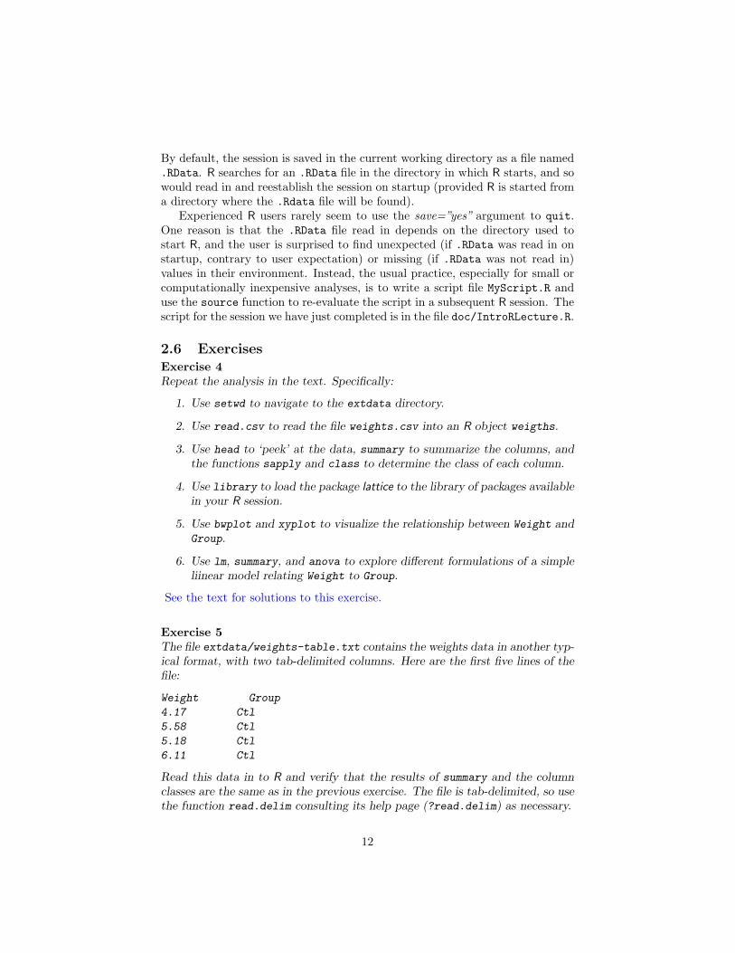
Exercise 5The file extdata/weights-table.txt contains the weights data in another typ-ical format, with two tab-delimited columns. Here are the first five lines of thefile:
Weight Group
4.17 Ctl
5.58 Ctl
5.18 Ctl
6.11 Ctl
Read this data in to R and verify that the results of summary and the columnclasses are the same as in the previous exercise. The file is tab-delimited, so usethe function read.delim consulting its help page (?read.delim) as necessary.
12
> wtsTable <- read.delim("extdata/weights-table.txt")
> head(wtsTable)
Weight Group1 4.17 Ctl2 5.58 Ctl3 5.18 Ctl4 6.11 Ctl5 4.50 Ctl6 4.61 Ctl
> summary(wtsTable)
Weight GroupMin. :3.590 Ctl:101st Qu.:4.388 Trt:10Median :4.750Mean :4.8463rd Qu.:5.218Max. :6.110
Exercise 6Both read.csv and read.delim are ‘wrappers’ around the function read.table.The wrappers are designed to make input of particular formats easy. How mustyou invoke read.delim to successfully input the csv-delimited data? The tab-delimited data?
> df1 <- read.table("extdata/weights.csv", header = TRUE,
+ sep = ",", row.names = 1)
> df2 <- read.table("extdata/weights-table.txt", header = TRUE)
Exercise 7R packages contain many ‘built-in’ data sets. Read in Fisher’s ‘iris’ data usingthe data command
> data(iris)
Read a brief description of the iris data set by consulting its help page withthe command ?iris.
1. Get a feeling for the data with head and summary. How many variablesand observations are there? What variables are present? What are theirclasses?
13
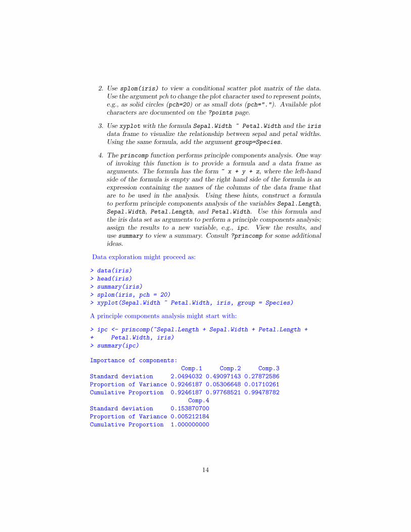
2. Use splom(iris) to view a conditional scatter plot matrix of the data.Use the argument pch to change the plot character used to represent points,e.g., as solid circles (pch=20) or as small dots (pch="."). Available plotcharacters are documented on the ?points page.
3. Use xyplot with the formula Sepal.Width ~ Petal.Width and the iris
data frame to visualize the relationship between sepal and petal widths.Using the same formula, add the argument group=Species.
4. The princomp function performs principle components analysis. One wayof invoking this function is to provide a formula and a data frame asarguments. The formula has the form ~ x + y + z, where the left-handside of the formula is empty and the right hand side of the formula is anexpression containing the names of the columns of the data frame thatare to be used in the analysis. Using these hints, construct a formulato perform principle components analysis of the variables Sepal.Length,Sepal.Width, Petal.Length, and Petal.Width. Use this formula andthe iris data set as arguments to perform a principle components analysis;assign the results to a new variable, e.g., ipc. View the results, anduse summary to view a summary. Consult ?princomp for some additionalideas.
Data exploration might proceed as:
> data(iris)
> head(iris)
> summary(iris)
> splom(iris, pch = 20)
> xyplot(Sepal.Width ~ Petal.Width, iris, group = Species)
A principle components analysis might start with:
> ipc <- princomp(~Sepal.Length + Sepal.Width + Petal.Length +
+ Petal.Width, iris)
> summary(ipc)
Importance of components:Comp.1 Comp.2 Comp.3
Standard deviation 2.0494032 0.49097143 0.27872586Proportion of Variance 0.9246187 0.05306648 0.01710261Cumulative Proportion 0.9246187 0.97768521 0.99478782
Comp.4Standard deviation 0.153870700Proportion of Variance 0.005212184Cumulative Proportion 1.000000000
14
3 The R programming language
This section highlights a few key features of the R programming language. Ad-ditional detail can be found in the R_intro_lecture.pdf file distributed withthese course notes, and in An Introduction to R.
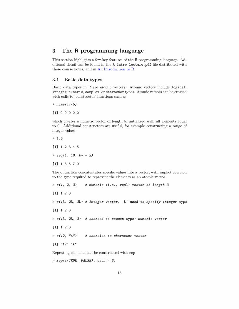
3.1 Basic data types
Basic data types in R are atomic vectors. Atomic vectors include logical,integer, numeric, complex, or character types. Atomic vectors can be createdwith calls to ‘constructor’ functions such as
> numeric(5)
[1] 0 0 0 0 0
which creates a numeric vector of length 5, initialized with all elements equalto 0. Additional constructors are useful, for example constructing a range ofinteger values
> 1:5
[1] 1 2 3 4 5
> seq(1, 10, by = 2)
[1] 1 3 5 7 9
The c function concatentates specific values into a vector, with implict coercionto the type required to represent the elements as an atomic vector.
> c(1, 2, 3) # numeric (i.e., real) vector of length 3
[1] 1 2 3
> c(1L, 2L, 3L) # integer vector, 'L' used to specify integer type
[1] 1 2 3
> c(1L, 2L, 3) # coerced to common type: numeric vector
[1] 1 2 3
> c(12, "A") # coercion to character vector
[1] "12" "A"
Repeating elements can be constructed with rep
> rep(c(TRUE, FALSE), each = 3)
15
[1] TRUE TRUE TRUE FALSE FALSE FALSE
R has useful pre-defined variables, e.g.,
> letters
[1] "a" "b" "c" "d" "e" "f" "g" "h" "i" "j" "k" "l" "m" "n" "o"[16] "p" "q" "r" "s" "t" "u" "v" "w" "x" "y" "z"
> pi
[1] 3.141593
Atomic vectors support standard programing concepts of Inf and NaN, but alsothe statistical concept of NA
> x <- c(1, Inf, -Inf, NaN, NA)
> x
[1] 1 Inf -Inf NaN NA
> typeof(x)
[1] "double"
> typeof(c(1L, NA))
[1] "integer"
The elements of atomic vectors can be named,
> x <- c(a = 1, b = 2)
> x
a b1 2
> names(x)
[1] "a" "b"
This can add very useful structure to simple data, and as illustrated belowcan facilitate element extraction. Coercion between types is often implict (e.g.,c(1L, 2L, 3) is coerced to type numeric), but can be made explicit.
> as.integer(c(1.41, 3.14))
[1] 1 3
16
R supports higher dimensional matrices (2-dimensional) and arrays (2 ormore dimensions). All elements of a matrix or array must be of the sameatomic type. A matrix can be constructed in many ways, but one way thatmakes R’s internal representation apparent is to start with a vector and specifydimensions, e.g.,
> matrix(1:12, nrow = 3)
[,1] [,2] [,3] [,4][1,] 1 4 7 10[2,] 2 5 8 11[3,] 3 6 9 12
Notice that the matrix is in column-major order; in fact, R represents the ma-trix as a vector, with addition attributes describing how the vector is to beinterpretted.
> attributes(matrix(1:12, nrow = 3))
$dim[1] 3 4
Row and column elements of matricies (and arrays) can be named, as can thedimension itself
> matrix(1:12, nrow = 3, dimnames = list(MyRows = LETTERS[1:3],
+ MyCols = letters[1:4]))
MyColsMyRows a b c d
A 1 4 7 10B 2 5 8 11C 3 6 9 12
This example uses a list. A list is a potentially heterogenous collection ofelements. The elements may be atomic or otherwise, including other lists. Listelements can be named.
> list(alpha = letters[1:4], ints = 1:4, m = matrix(1:12,
+ nrow = 3))
$alpha[1] "a" "b" "c" "d"
$ints[1] 1 2 3 4
$m[,1] [,2] [,3] [,4]
17
[1,] 1 4 7 10[2,] 2 5 8 11[3,] 3 6 9 12
We have already had extensive contact with the data.frame, which is a specialtype of list. A data frame is a list, with the restriction that each element of thelist must be an atomic type, and that all elements must be the same length. Adata frame is constructed as, for instance,
> data.frame(alpha = letters[1:4], ints = 1:4)
alpha ints1 a 12 b 23 c 34 d 4
An environment is like a list, in that it can store heterogenous collections ofvalues. Unlike lists, all elements of an environment must be named. And aswill become apparent below, environments are almost unique amongst R datastructures in providing pass by reference semantics rather than pass by value.An environment is one way to represent an efficient hash table.
A final and perhaps surprising data type on our tour is the function. Userscreate a function by providing an argument list and body consisting of linesof valid R code. A function returns the value of the last line it executes, so noexplicit return statement is needed. Users typically assign functions to variablesthat can then be manipulated by other variables. Here is a simple function thattakes one argument, x , and squares it. The squared value is the last line (andthe first!) of the function that is executed, and is thus the value returned bythe function.
> square <- function(x) {
+ x * x
+ }
We’ll see that arithemtic operations are vectorized, so our square function workson vectors too.
> square(1:4)
[1] 1 4 9 16
Notice that our square is as much a function as any other function in R, andso can be used in, for instance, other functions like sapply (here, sapply istaking each element of its first argument, and applying the function in its secondargument to the element; what happens in the second line, below?).
> sapply(list(1:4, 3:1), square)
18
[[1]][1] 1 4 9 16
[[2]][1] 9 4 1
> sapply(sapply(list(1:4, 3:1), square), sum)
[1] 30 14
3.2 Subsetting
One of the most common operations associated with atomic and other objectsis subsetting. We have already seen this to some extent, for instance in selectingthe first four entries of the character variable letters. For any atomic vectorwe can subset using positive integers, in any order, to select the correspondingelement. We can also select outside the range of the vector index to extend thevector (though this is not usually a good idea). Negative indices remove thecorresponding entries; positive and negative indices cannot be used in the samestep.
> letters[c(2:3, 15:17, 18:16)]
[1] "b" "c" "o" "p" "q" "r" "q" "p"
> letters[25:28]
[1] "y" "z" NA NA
> letters[-c(1:20)]
[1] "u" "v" "w" "x" "y" "z"
When atomic types or lists contain named elements, the name can be used toretrieve a specific element.
> x <- c(a = 1, b = 2, c = 3)
> x[c("a", "c")]
a c1 3
Logical vectors can be used for subsetting, and have the useful property thatthey are recycled to match the length of the object they are subsetting. So fora vector of length 10 we can choose every third element with
> x <- 1:10
> x[c(FALSE, FALSE, TRUE)]
19
[1] 3 6 9
We have seen, e.g., in square, that arithmetic operations are vectorized. Soone way of chosing values of a vector that are, say, divisible by 3 might beto construct a logical index from the appropriate comparison, e.g., using themodulus operator %%
> x <- c(1, 3, 6:9)
> idx <- x%%3 == 0
> idx
[1] FALSE TRUE TRUE FALSE FALSE TRUE
> x[idx]
[1] 3 6 9
This would often be abbreviated into the one-liner x[x %% 3 == 0].Subsetting extends to matrices and arrays, with a two-dimension comma-
separated subscript (for a matrix) replacing the single subscript for a vector.A subscript can be missing, in which case all the corresponding elements ofthat dimension (all rows, for instance) are selected. Dimensions can be subsetdifferently, e.g., rows subset by negative integer values, columns by logical valuesor names.
> m <- matrix(1:12, nrow = 3)
> m[1:2, -3]
[,1] [,2] [,3][1,] 1 4 10[2,] 2 5 11
Selecting a single row or column of a matrix will return a vector, unless theoptional argument drop is set to FALSE
> m[1, ]
[1] 1 4 7 10
> m[1, , drop = FALSE]
[,1] [,2] [,3] [,4][1,] 1 4 7 10
Elements of vectors or matrices can be replaced using subsetting on the leftside of the assignment operator.
> x <- 1:3
> x[2] <- 4
> x
20
[1] 1 4 3
Note that R usually has pass by value semantics. This means that changing oneobject does not change any copies of that object:
> x <- 1:3
> y <- x # x and y 'the same', i.e., numerically equal
> x[2] <- 4 # change x
> x # x changed
[1] 1 4 3
> y # not y
[1] 1 2 3
A final subsetting operation involves the ’double-subset’, [[. The distinctionbetween this and the single subset operator [ is primarily apparent with lists andenvironments. With a list, the single subset returns a list containing the specifiedelements. With the double subset, only a single element can be specified, andthe result is the element itself and not a list. In the following, the first operationreturns a list containing a matrix, the double subset returns the matrix itself.
> l <- list(m = matrix(1:12, nrow = 3), n = 1:5)
> l
$m[,1] [,2] [,3] [,4]
[1,] 1 4 7 10[2,] 2 5 8 11[3,] 3 6 9 12
$n[1] 1 2 3 4 5
> l["m"]
$m[,1] [,2] [,3] [,4]
[1,] 1 4 7 10[2,] 2 5 8 11[3,] 3 6 9 12
> l[["m"]]
[,1] [,2] [,3] [,4][1,] 1 4 7 10[2,] 2 5 8 11[3,] 3 6 9 12
21
Environments can only be subset using the double subset operator, and must besubset using a character vector to identify a named element. Assignment usingdouble subsetting is like that for single subsetting on lists; environments havepass by reference semantics and assignment has the side effect of modifying anycopy of the environment. This is generally surprising behavior to the user, soenvironments are used only in specific circumstances.
> env <- new.env() # create a new environment, see ?new.env
> env[["x"]] <- 1 # create an element "x", and assign value 1 to it
> env[["x"]]
[1] 1
> env_copy <- env # make a copy of the environment
> env[["x"]] <- 2 # change the original
> env[["x"]] # env modified
[1] 2
> env_copy[["x"]] # but so is env_copy!
[1] 2
3.3 Useful programming operations
R supports a complete range of built-in operations for manipulating numeri-cal (e.g., +, sqrt, abs, exp, cos), logical (e.g., ! for logical negation, anyto test whether any element of a logical vector is TRUE), and character (e.g.,nchar, gsub, substr) data. R has additional functions useful for statisticalanalysis (e.g., rnorm for generating normal random deviates; combn for generat-ing all combinations of elements, intersect to calculate the intersection of twovectors). A distinct feature of R is that many of these operations are vectorized,so that ‘looping through a vector’ is often unnecessary (and very inefficient).Arithmetic operations use recycling, so that in the first line the vector 1 is (con-ceptually) expanded to a vector of length five, and then added element-wise tothe square root of the numbers 1 through 5.
> log(1 + sqrt(1:5))
[1] 0.6931472 0.8813736 1.0050525 1.0986123 1.1743590
> dev <- rnorm(100)
> max(dev)
[1] 2.486159
> any(dev > 2)
[1] TRUE
22
> sum(dev > 2)
[1] 1
> s <- c("Fred", "Frank")
> sub("F", "G", s)
[1] "Gred" "Grank"
Specifics of these functions are found on their help pages, e.g., ?any.R supports all common programming constructs. For instance, conditional
evaluation occurs with if:
> dev <- rnorm(100)
> if (any(dev > 2)) {
+ cat("some deviates greater than 2\n")
+ } else {
+ cat("hmm, all deviates less than 2\n")
+ }
some deviates greater than 2
Braces are used to group multiple lines of code into a single expression.Iteration over vectors uses for:
> for (i in 2:1) {
+ cat("I am", i, "\n")
+ }
I am 2I am 1
> lst <- list(a = 1, b = 2)
> for (elt in lst) {
+ cat("I am", elt, "\n")
+ }
I am 1I am 2
The second example shows that iteration is over elements of atomic vectors.When a for loop is used to assign elements to a vector, it is efficient to ‘pre-allocate’
> results <- numeric(10000)
> for (i in seq_along(results)) {
+ results[[i]] <- aFancyCalculation()
+ }
23
Conversely, sapply or lapply is often a better choice when the task is to iterateover a set of values, e.g.,
> cls1 <- sapply(iris, class)
instead of
> cls2 <- character(ncol(iris))
> for (i in seq_along(cls2)) {
+ cls2[[i]] <- class(iris[[i]])
+ }
> names(cls2) <- names(iris)
> identical(cls1, cls2)
[1] TRUE
More detail about R syntax can be found with ?Syntax. Details on pro-gramming language constructs can be found with ?if, etc. The manual AnIntroduction to R is a useful starting point.
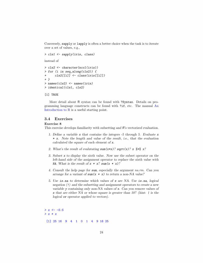
3.4 ExercisesExercise 8This exercise develops familiarity with subsetting and R’s vectorized evaluation.
1. Define a variable x that contains the integers -5 through 5. Evaluate x
* x. Note the length and value of the result, i.e., that the evaluationcalculated the square of each element of x.
2. What’s the result of evalutating sum(x*x)? sqrt(x)? x %*% x?
3. Subset x to display the sixth value. Now use the subset operator on theleft-hand side of the assignment operator to replace the sixth value withNA. What is the result of x * x? sum(x * x)?
4. Consult the help page for sum, especially the argument na.rm. Can youarrange for a variant of sum(x * x) to return a non-NA value?
5. Use is.na to determine which values of x are NA. Use is.na, logicalnegation (!) and the subsetting and assignment operators to create a newvariable y containing only non-NA values of x. Can you remove values ofx that are either NA or whose square is greater than 10? (hint: | is thelogical or operator applied to vectors).
> x <- -5:5
> x * x
[1] 25 16 9 4 1 0 1 4 9 16 25
24
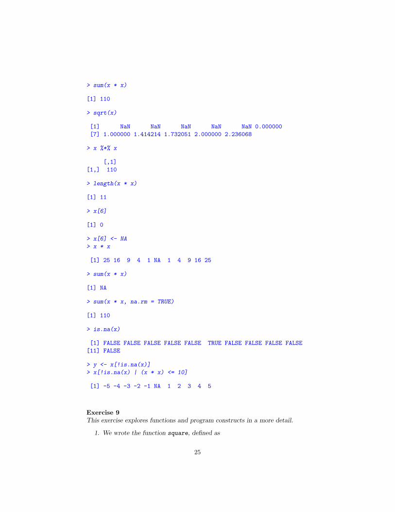
> sum(x * x)
[1] 110
> sqrt(x)
[1] NaN NaN NaN NaN NaN 0.000000[7] 1.000000 1.414214 1.732051 2.000000 2.236068
> x %*% x
[,1][1,] 110
> length(x * x)
[1] 11
> x[6]
[1] 0
> x[6] <- NA
> x * x
[1] 25 16 9 4 1 NA 1 4 9 16 25
> sum(x * x)
[1] NA
> sum(x * x, na.rm = TRUE)
[1] 110
> is.na(x)
[1] FALSE FALSE FALSE FALSE FALSE TRUE FALSE FALSE FALSE FALSE[11] FALSE
> y <- x[!is.na(x)]
> x[!is.na(x) | (x * x) <= 10]
[1] -5 -4 -3 -2 -1 NA 1 2 3 4 5
Exercise 9This exercise explores functions and program constructs in a more detail.
1. We wrote the function square, defined as
25
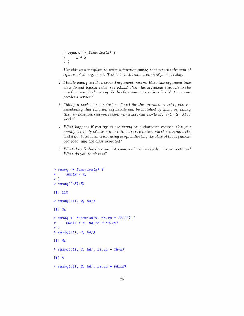
> square <- function(x) {
+ x * x
+ }
Use this as a template to write a function sumsq that returns the sum ofsquares of its argument. Test this with some vectors of your chosing.
2. Modify sumsq to take a second argument, na.rm. Have this argument takeon a default logical value, say FALSE. Pass this argument through to thesum function inside sumsq. Is this function more or less flexible than yourprevious version?
3. Taking a peek at the solution offered for the previous exercise, and re-membering that function arguments can be matched by name or, failingthat, by position, can you reason why sumsq(na.rm=TRUE, c(1, 2, NA))
works?
4. What happens if you try to use sumsq on a character vector? Can youmodify the body of sumsq to use is.numeric to test whether x is numeric,and if not to issue an error, using stop, indicating the class of the argumentprovided, and the class expected?
5. What does R think the sum of squares of a zero-length numeric vector is?What do you think it is?
> sumsq <- function(x) {
+ sum(x * x)
+ }
> sumsq((-5):5)
[1] 110
> sumsq(c(1, 2, NA))
[1] NA
> sumsq <- function(x, na.rm = FALSE) {
+ sum(x * x, na.rm = na.rm)
+ }
> sumsq(c(1, 2, NA))
[1] NA
> sumsq(c(1, 2, NA), na.rm = TRUE)
[1] 5
> sumsq(c(1, 2, NA), na.rm = FALSE)
26
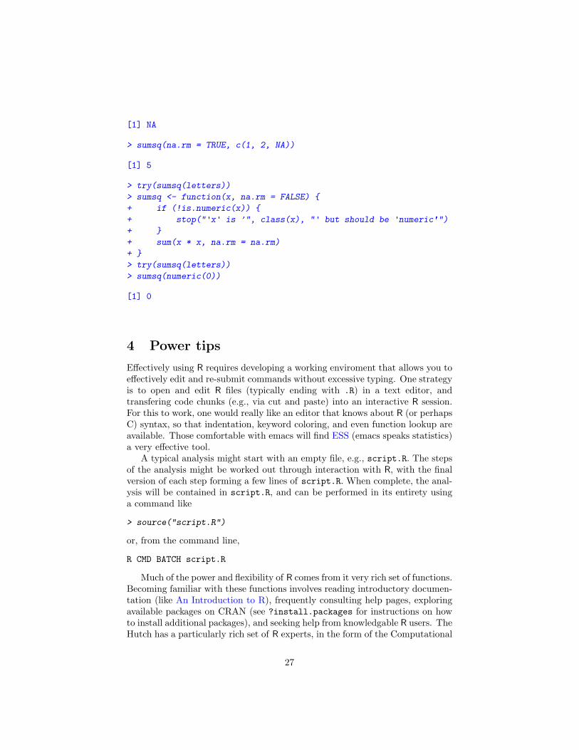
[1] NA
> sumsq(na.rm = TRUE, c(1, 2, NA))
[1] 5
> try(sumsq(letters))
> sumsq <- function(x, na.rm = FALSE) {
+ if (!is.numeric(x)) {
+ stop("'x' is '", class(x), "' but should be 'numeric'")
+ }
+ sum(x * x, na.rm = na.rm)
+ }
> try(sumsq(letters))
> sumsq(numeric(0))
[1] 0
4 Power tips
Effectively using R requires developing a working enviroment that allows you toeffectively edit and re-submit commands without excessive typing. One strategyis to open and edit R files (typically ending with .R) in a text editor, andtransfering code chunks (e.g., via cut and paste) into an interactive R session.For this to work, one would really like an editor that knows about R (or perhapsC) syntax, so that indentation, keyword coloring, and even function lookup areavailable. Those comfortable with emacs will find ESS (emacs speaks statistics)a very effective tool.
A typical analysis might start with an empty file, e.g., script.R. The stepsof the analysis might be worked out through interaction with R, with the finalversion of each step forming a few lines of script.R. When complete, the anal-ysis will be contained in script.R, and can be performed in its entirety usinga command like
> source("script.R")
or, from the command line,
R CMD BATCH script.R
Much of the power and flexibility of R comes from it very rich set of functions.Becoming familiar with these functions involves reading introductory documen-tation (like An Introduction to R), frequently consulting help pages, exploringavailable packages on CRAN (see ?install.packages for instructions on howto install additional packages), and seeking help from knowledgable R users. TheHutch has a particularly rich set of R experts, in the form of the Computational
27

Biology Shared Resource and more generally members of the ComputationalBiology program involved in the BioConductor project. The R-help mailing listis invaluable both as an archive of previous questions and a resource for gettingusually helpful, friendly, and accurate advice.
28