An Introduction to Proof Complexity, Part II. · Let TAUT be a set of tautologies. A proof system for TAUT is any polynomial time computable function f that maps the set of all binary

An Introduction to Proof Complexity,Part II.

Pavel PudlakMathematical Institute, Academy of Sciences, Prague

andCharles University, Prague

Computability in Europe 2009, Heidelberg

1

Overview

Part I.

A lower bound for the propositional Pigeon-Hole Principle.

Theories and complexity classes.

Conditional and relativized separation of theories.

Part II.

Propositional proof systems.

Feasible interpolation.

Unprovability of circuit lower bounds.

Total search problems. (not presented at CiE)

Feasible incompleteness. (not presented at CiE)

2

Propositional Proof Systems

The idea of a general propositional proof system

1 it is sound;

2 it is complete;

3 the relation ‘D is a proof of tautology φ” is decidable in polynomial time.

Definition (Cook, 1975)

Let TAUT be a set of tautologies. A proof system for TAUT is any polynomialtime computable function f that maps the set of all binary strings {0, 1}∗ ontoTAUT .

Meaning:Every string is a proof.f (a) is the formula of which a is a proof.

Say that a proof system is polynomially bounded, if every tautology has a proof ofpolynomial length.

FactThere exists a polynomially bounded proof system iff NP = coNP.

3


DefinitionA proof system f1 polynomially simulates a proof system f2, if there exists apolynomial time computable function g such that for all a ∈ {0, 1}∗,f1(g(a)) = f2(a).

Meaning:Given a proof a of f2(a) in the second system, we can construct a proof g(a) ofthe same tautology in the first system in polynomial time.

Theorem (Cook-Reckhow)

Frege systems polynomially simulate each other.

4


DefinitionA proof system f1 polynomially simulates a proof system f2, if there exists apolynomial time computable function g such that for all a ∈ {0, 1}∗,f1(g(a)) = f2(a).

Meaning:Given a proof a of f2(a) in the second system, we can construct a proof g(a) ofthe same tautology in the first system in polynomial time.

Theorem (Cook-Reckhow)

Frege systems polynomially simulate each other.

4

Extended Frege proof systems

Extension Rule: Whenever needed, introduce formula

p ≡ φ,

where p is a new variable that does not occur in the conclusion nor in φ and φ isotherwise arbitrary.

An Extended Frege proof system is a Frege system augmented with the extensionrule.

Extended Frege systems polynomially simulate each other.

Extended Frege systems are polynomially equivalent to

1. Substitution Frege systems—Frege systems with the substitution rule.

2. Circuit Frege systems—Frege systems that use boolean circuits instead offormulas.

5

Extended Frege proof systems are the strongest proof systems whose soundnessΘP proves.

Theorem (Cook, 1975)

If P is a proof system whose soundness is provable in ΘP, then Extended Fregeproof systems polynomially simulate P.

In principle it is possible to prove ΘP 6= ΘNP by proving superpolynomial lowerbounds on Extended Frege proofs of explicitly defined tautologies.

Corollary

Suppose T is a polynomial time decidable set of tautologies such that tautologiesfrom T do not have polynomial size proofs in an Extended Frege proof system.Further suppose that ΘNP proves that every element of T is a tautology. ThenΘP 6= ΘNP.

6

TheoremIf Extended Frege proof systems are not polynomially bounded, thenΘP 6` P = NP.

More presicely, we have the following stronger theorem:

If there exists no polynomial time algorithm that for a given tautology constructsan extended frege proof, then for no Πb

1 formula φ(x), ΘP ` ∀x Sat(x) ≡ φ(x).

Proof. Suppose ΘP ` ∀x Sat(x) ≡ φ(x). Then

ΘP ` ∀x Sat(x) ∨ ¬φ(x).

Since Sat(x) ∨ ¬φ(x) is a Σb1 formula, by Buss’s Theorem the existential

quantifiers can be witnessed by a polynomial time computable function.

Since ¬φ(¬x) ≡ ¬Sat(¬x), the formula ¬φ(¬x) defines a plynomially boundedproof system.

By Cook’s theorem, this proof system is polynomially simulated by an ExtendedFrege system.

Hence proofs in an Extenden Frege system can be found in polynomial time.

7

Some propositional proof systems

Resolution

depth 2 Frege systems

depth 3 Frege systems

...

............................. ↑ exp. lower bounds

Frege systems

Extended Frege systems

8

Feasible interpolation

Theorem (Craig)

Let Φ(p, q)→ Ψ(p, r) be a tautology, where p, q, r are disjoint sets ofpropositional variables, there exists a formula I (p), which contains only thecommon variables p, such that both Φ(p, q)→ I (p) and I (p)→ Ψ(p, r) aretautologies.

Krajıcek’s Idea: If we have a short proof of Φ(p, q)→ Ψ(p, r), we can bound thecomplexity of I (p).Thus we could reduce proving lower bounds on the lengths of proofs to lowerbounds on circuit complexity.

This idea does not work for all proof systems. If it works, we say that the proofsystem has the feasible interpolation property.

9

Φ(p, q)→ I (p) and I (p)→ Ψ(p, r)

is equivalent toΦ(p, q)→ I (p) and ¬Ψ(p, r)→ I (p),

hence also to

∃q Φ(p, q)→ I (p) and ∃r ¬Ψ(p, r)→ ¬I (p).

AlsoΦ(p, q)→ Ψ(p, r)

is equivalent to¬∃p (∃q Φ(p, q) ∧ ∃r ¬Ψ(p, r)).

Theorem (informal statement)

If A,B ∈ NP such that Resolution proves A ∩ B = ∅ using proofs of polynomialsize, then A and B can be separated by a set C ∈ P/poly.

10

Resolution is the proof system which uses elementary disjunctions i.e.,disjunctions of literals, as formulas, and the cut rule as the only rule

Γ ∨ p, ∆ ∨ ¬p

Γ ∨∆,

(where Γ,∆ are elementary disjunctions).A literal is a variable or a negated variable.Elementary disjunctions are called clauses.

The ternary connective sel (selector) is defined by sel(0, x , y) = x andsel(1, x , y) = y .

11

Resolution is the proof system which uses elementary disjunctions i.e.,disjunctions of literals, as formulas, and the cut rule as the only rule

Γ ∨ p, ∆ ∨ ¬p

Γ ∨∆,

(where Γ,∆ are elementary disjunctions).A literal is a variable or a negated variable.Elementary disjunctions are called clauses.

The ternary connective sel (selector) is defined by sel(0, x , y) = x andsel(1, x , y) = y .

11

Theorem (essentially - Krajıcek, 1994)

Let P be a resolution proof of the empty clause from clauses Ai (p, q), i ∈ I ,Bj(p, r), j ∈ J where p, q, r are disjoint sets of propositional variables. Then thereexists a circuit C (p) such that for every 0-1 assignment a for p

C (a) = 0 ⇒ Ai (a, q), i ∈ I are unsatisfiable, and

C (a) = 1 ⇒ Bj(a, r), j ∈ J are unsatisfiable;

the circuit C is in basis {0, 1,∧,∨, sel} and its underlying graph is the graph ofthe proof P.

Moreover, we can construct in polynomial time a resolution proof of the emptyclause from clauses Ai (a, q), i ∈ I if C (a) = 0, respectively Bj(a, r), j ∈ J ifC (a) = 1; the length of this proof is less than or equal to the length of P.

12

Theorem (essentially - Krajıcek, 1994)

Let P be a resolution proof of the empty clause from clauses Ai (p, q), i ∈ I ,Bj(p, r), j ∈ J where p, q, r are disjoint sets of propositional variables. Then thereexists a circuit C (p) such that for every 0-1 assignment a for p



the circuit C is in basis {0, 1,∧,∨, sel} and its underlying graph is the graph ofthe proof P.Moreover, we can construct in polynomial time a resolution proof of the emptyclause from clauses Ai (a, q), i ∈ I if C (a) = 0, respectively Bj(a, r), j ∈ J ifC (a) = 1; the length of this proof is less than or equal to the length of P.

12

The idea of the proof.

. . .Ai (p, q) . . . . . .Bj(p, r) . . .. . . . . .. . .∅

Given an assignment a for p, follow the proof but instead of resolving on variablespi just substitute for them.

Thus the proof splits into two parts: one with only variables q the other withvariables r .

One of the parts contains the empty clause—this is the refutation of thecorresponding part of initial clauses. E.g.

. . .Ai (a, q) . . . . . .Bj(a, r) . . .. . . . . .. . . . . .∅

Thus we have a polynomial time algorithm for deciding which set of clauses isinconsistent.

13

Proof.

First we describe the transformation of the proof for a given assignment p 7→ a.Once we get an assignment for p, we can eliminate all these variables from theproof, but we shall do it in two stages, as we shall need more information aboutthis process when constructing the circuit explicitly.

Let us call a clause q-clause, resp. r-clause, if it contains only variables p, q resp.p, r . We shall call a clause q-clause, resp. r-clause also in the case that the clausecontains only variables p or is empty, but its ancestors are q-clauses, resp.r-clauses.

1. In the first stage we replace each clause of P by a subclause so that eachclause in the proof is either q-clause or r-clause. We start with the initial clauses,which are left unchanged and continue along the derivation P.

Case 1.Γ ∨ pk , ∆ ∨ ¬pk

Γ ∨∆

and we have replaced Γ∨ pk by Γ′ and ∆∨¬pk by ∆′. Then we replace Γ∨∆ byΓ′ if pk 7→ 0 and by ∆′ if pk 7→ 1.

14

Case 2.Γ ∨ qk , ∆ ∨ ¬qk

Γ ∨∆

and we have replaced Γ ∨ qk by Γ′ and ∆ ∨ ¬qk by ∆′. If one of Γ′, ∆′ is anr-clause, then it does not contain qk , and we replace Γ ∨∆ by this clause. If bothΓ′ and ∆′ are q-clauses, we resolve along qk , or take one, which does notcontain qk .

Case 3.Γ ∨ rk , ∆ ∨ ¬rk

Γ ∨∆.

This is the dual case to case 2.

2. Now delete the clauses which contain a p literal with value 1, and remove all pliterals from the remaining clauses. Thus we get a valid derivation of the finalempty clause from the reduced initial clauses. If this final clause is a q-clause, theproof contains a subproof using only the reduced clauses Ai , i ∈ I ; if it is anr-clause, the proof contains a subproof using only the reduced clauses Bj , j ∈ J.

15

3. The circuit C is constructed so that the value computed at a gatecorresponding to a clause Γ will determine if it is transformed into a q-clause oran r-clause. We assign 0 to q-clauses and 1 to r-clauses.Thus the circuit is constructed as follows. Put constant 0 gates on clausesAi , i ∈ I and constant 1 gates on clauses Bj , j ∈ J. Now consider three cases asabove.

Case 1. If the gate on Γ ∨ pk gets value x and the gate on ∆ ∨ ¬pk gets value y ,then the gate on Γ ∨∆ should get the value z = sel(pk , x , y). Thus we place thesel gate on Γ ∨∆.

Case 2. If the gate on Γ ∨ qk gets value x and the gate on ∆ ∨ ¬qk gets value y ,then the gate on Γ ∨∆ should get the value z = x ∨ y . Thus we place the ∨ gateon Γ ∨∆.

Case 3. This is dual to case 2, so we place the ∧ gate on Γ ∨∆.

16

We cannot prove lower bounds using this theorem without using unprovenassumptions, because we are not able to prove lower bounds on the size ofboolean circuits.

17

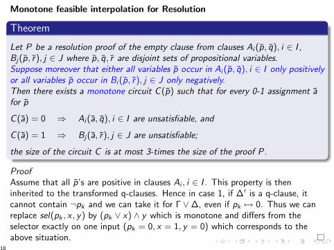
Monotone feasible interpolation for Resolution

Theorem

Let P be a resolution proof of the empty clause from clauses Ai (p, q), i ∈ I ,Bj(p, r), j ∈ J where p, q, r are disjoint sets of propositional variables.Suppose moreover that either all variables p occur in Ai (p, q), i ∈ I only positivelyor all variables p occur in Bi (p, r), j ∈ J only negatively.Then there exists a monotone circuit C (p) such that for every 0-1 assignment afor p



the size of the circuit C is at most 3-times the size of the proof P.

ProofAssume that all p’s are positive in clauses Ai , i ∈ I . This property is theninherited to the transformed q-clauses. Hence in case 1, if ∆′ is a q-clause, itcannot contain ¬pk and we can take it for Γ ∨∆, even if pk 7→ 0. Thus we canreplace sel(pk , x , y) by (pk ∨ x) ∧ y which is monotone and differs from theselector exactly on one input (pk = 0, x = 1, y = 0) which corresponds to theabove situation.

18

Application — an exponential lower bound on Resolution proofs

A. Haken, 1985, an exponential lower bound on Resolution proofs of PHP.A.A. Razborov, 1985, an exponential lower bound on monotone circuits.

Theorem (Razborov, Boppana-Alon)

Let m =(n2

), let k = n1/4. Think of a ∈ {0, 1}m as graphs on n vertices.

Let C be a monotone boolean circuit with m input variables such that

a encodes a graph with a clique of size k ⇒ C (a) = 1,

a encodes a k − 1 colorable graph ⇒ C (a) = 0.

Then the size of C is at least 2nε

.

Corollary

Let Φ(p, q) express “ q is not a clique of size k in graph p ”,Let Ψ(p, r) express “ r is not a k − 1-coloring of graph p ”.Then every Resolution proof of the tautology Φ(p, q) ∨Ψ(p, r) has sizeat least 1

32nε

.

19

DefinitionA proof system P has the feasible interpolation property, if there is a polynomialtime algorithm such that given an implication of the form φ(p, q)→ ψ(p, r) andits proof d in the proof system P, the algorithm constructs a circuit C (p) thatinterpolates the implication. In particular, the size of the circuit C is bounded bya polynomial in the length of the proof d .

Proof systems with the feasible interpolation property

Polynomial Calculus

Cutting Planes

Lovasz-Schrijver

Proof systems that do not have the feasible interpolation property

Assuming that factoring is hard:

bounded depth Frege and stronger systems

20



Polynomial Calculus

Cutting Planes

Lovasz-Schrijver




20



Polynomial Calculus

Cutting Planes

Lovasz-Schrijver




20

Monotone interpolation for Cutting Planes

Cutting planes proof system

Propositional variables p1, p2, . . . with the interpretation 0 = false and 1 = true.A proof line is an inequality ∑

k

ckpk ≥ C ,

where ck and C are integers.

The axioms are pk ≥ 0 and −pk ≥ −1 (i.e. 0 ≤ pk ≤ 1) for every propositionalvariable pk .The rules are

1 addition: from∑

k ckpk ≥ C and∑

k dkpk ≥ D derive∑k(ck + dk)pk ≥ C + D;

2 multiplication: from∑

k ckpk ≥ C derive∑

k dckpk ≥ dC , where d is anarbitrary positive integer;

3 division: from∑

k ckpk ≥ C derive∑

kck

d pk ≥⌈

Cd

⌉, provided that d > 0 is

an integer which divides each ck .

21

DefinitionA monotone real circuit is a circuit which computes with real numbers and usesarbitrary nondecreasing real unary and binary functions as gates.We say that a monotone real circuit computes a boolean function, if for all inputsof 0’s and 1’s the circuit outputs 0 or 1.

Examples of monotone real gates: max,min,+, ex ; also × on R+.

Theorem (Pudlak 1997)

Let P be a cutting plane proof of the contradiction 0 ≥ 1 from inequalities∑k

ci,kpk +∑

l

bi,lql ≥ Ai , i ∈ I ,

∑k

c ′j,kpk +∑m

dj,mrm ≥ Bj , j ∈ J.

Suppose that all the coefficients ci,k are nonnegative, or all the coefficients c ′i,kare nonpositive, then one can construct a real monotone interpolating circuit C(computing a boolean function) whose size is bounded by a linear function in thenumber of variables and the number of inequalities of the proof P.

22

Theorem (Pudlak 1997)

Let m =(n2

), let k = n1/4.

Let C be a monotone real circuit with m input variables such that

a encodes a graph with a clique of size k ⇒ C (a) = 1,

a encodes a k − 1 colorable graph ⇒ C (a) = 0.

Then the size of C is at least 2nδ

.

Corollary

Let Φ(p, q) express “ q is not a clique of size k in graph p ”,Let Ψ(p, r) express “ r is not a k − 1-coloring of graph p ”.Then every Cutting-Planes proof of the tautology Φ(p, q) ∨Ψ(p, r) has size

at least 2nδ

.

Independently, Cook and Haken proved similar bounds for Broken MosquitoScreen pair of disjoint NP sets.

23

Corollary

No algorithm based only on cutting planes can solve the Integer LinearPrograming problem in subexponential time.

Corollary (of the lower bounds on tree-like resolution proofs)

No algorithm based Davis-Putnam procedure can solve 3− SAT in time less than2ε for some ε > 0.

24

Corollary

No algorithm based only on cutting planes can solve the Integer LinearPrograming problem in subexponential time.

Corollary (of the lower bounds on tree-like resolution proofs)

No algorithm based Davis-Putnam procedure can solve 3− SAT in time less than2ε for some ε > 0.

24

Monotone boolean circuits

type of circuit lower bounds proof systemmonotone circuits with ∧,∨ yes Resolutionreal monotone circuits yes Cutting Planesmonotone span programs yes Polynomial Calculusmonotone linear programs no Lovasz-Schrijver??? ???

A monotone LP programs P:∑j

aijzj ≤∑

k

bikxk + ci

aij , bi,k , ci ∈ R constants; zj ∈ R+, xk ∈ {0, 1} variables

P computes boolean function f (x), if for every assignment to x

P has a solution z ⇔ f (x) = 1

Monotone LP polynomially simulate monotone circuits and monotone spanprograms over reals.

25

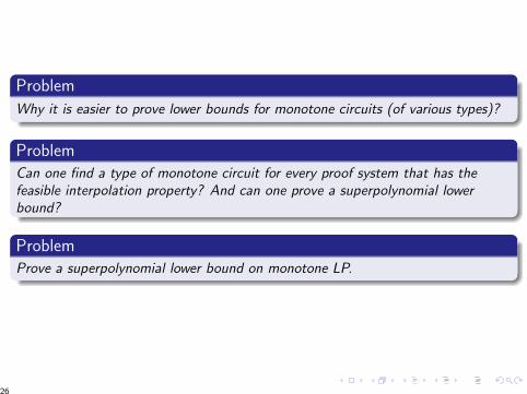
Problem

Why it is easier to prove lower bounds for monotone circuits (of various types)?

ProblemCan one find a type of monotone circuit for every proof system that has thefeasible interpolation property? And can one prove a superpolynomial lowerbound?

ProblemProve a superpolynomial lower bound on monotone LP.

26

Unprovability of circuit lower bounds

Theorem (Razborov 1995, Krajıcek)

Assuming PRG-Conjecture the following is true. If P is a propositional proofsystem with the feasible interpolation property, then for every boolean function fit is hard to prove in P an exponential lower bound on the circuit complexity of f .

PRG-ConjectureThere exists an ε > 0 and a polynomial time computable function (the PRGgenerator) Gn : {0, 1}n → {0, 1}2n such that for every circuit C of size ≤ 2nε

|Prob(C (Gn(x))) = 1− Prob(C (y) = 1)| ≥ 2−nε

.

Theorem (Razborov-Rudich,1994)

PRG-Conjecture implies that there is no polynomial time computable property ofboolean functions that implies superpolynomial lower bounds and is satisfied by≥ 1/2 of all boolean functions.

View a boolean function of n variables as a 0-1 string of length 2n.

PRG-Conjecture ⇒ there exists a pseudorandom function generator.

27

Unprovability of circuit lower bounds

Theorem (Razborov 1995, Krajıcek)

Assuming PRG-Conjecture the following is true. If P is a propositional proofsystem with the feasible interpolation property, then for every boolean function fit is hard to prove in P an exponential lower bound on the circuit complexity of f .

PRG-ConjectureThere exists an ε > 0 and a polynomial time computable function (the PRGgenerator) Gn : {0, 1}n → {0, 1}2n such that for every circuit C of size ≤ 2nε

|Prob(C (Gn(x))) = 1− Prob(C (y) = 1)| ≥ 2−nε

.

Theorem (Razborov-Rudich,1994)

PRG-Conjecture implies that there is no polynomial time computable property ofboolean functions that implies superpolynomial lower bounds and is satisfied by≥ 1/2 of all boolean functions.

View a boolean function of n variables as a 0-1 string of length 2n.

PRG-Conjecture ⇒ there exists a pseudorandom function generator.27

IdeaLet N = 2n. Think of x ∈ {0, 1}N as boolean functions of n variables.Let αM(p, q) be a boolean formula expressing:

“the function coded by p has a circuit of size M (coded by q)”

Thus |p| = N and |q| ≈ M log M.

Suppose P is a proof system with the feasible interpolation property.Suppose for some function a ∈ {0, 1}N , there is a poly-size P-proof of the circuitlower bound 2M + 1, i.e., of the tautology ¬α2M+1(a, q).Then we also have a poly-size proof of

¬αM(p, q) ∨ ¬αM(p ⊕ a, r).

By feasible interpolation, there exists a poly-size circuit C such that for allb ∈ {0, 1}N

C (b) = 0 ⇒ ¬αM(b, q)

C (b) = 1 ⇒ ¬αM(b ⊕ a, r)

28

IdeaLet N = 2n. Think of x ∈ {0, 1}N as boolean functions of n variables.Let αM(p, q) be a boolean formula expressing:

“the function coded by p has a circuit of size M (coded by q)”

Thus |p| = N and |q| ≈ M log M.

Suppose P is a proof system with the feasible interpolation property.Suppose for some function a ∈ {0, 1}N , there is a poly-size P-proof of the circuitlower bound 2M + 1, i.e., of the tautology ¬α2M+1(a, q).Then we also have a poly-size proof of

¬αM(p, q) ∨ ¬αM(p ⊕ a, r).

By feasible interpolation, there exists a poly-size circuit C such that for allb ∈ {0, 1}N

C (b) = 0 ⇒ ¬αM(b, q)

C (b) = 1 ⇒ ¬αM(b ⊕ a, r)

28

C (b) = 0 ⇒ ¬αM(b, q)

C (b) = 1 ⇒ ¬αM(b ⊕ a, r)

Hence:

if |{b; C (b) = 0}| ≥ 122N , then “C (x) = 0” defines a property of functions

of complexity ≥ M satisfied by 1/2 of all functions,

otherwise “C (x ⊕ a) = 1” is such a property.

Assuming the PRG-Conjecture, if M is superpolynomial in n (i.e., M = nω(1)),then this is not possible.So it is not possible to prove a superpolynomial lower bound using a polynomialsize proof (i.e. of size Nc = 2cn for c constant).

TheoremAssume the PRG-Conjecture. If a proof system P has the feasible interpolationproperty, then there are no polynomial size P-proofs of superpolynomial circuitlower bounds.

29


Theorem (Krajıcek 2004)

Superpolynomial circuit lower bounds are hard for Resolution.

Without PRG-Conjecture!

ProblemFeasible interpolation holds only for weak propositional proof systems. Can oneprove such lower bounds for other propositional proof systems?

Likely for bounded depth Frege systems.

30


Theorem (Krajıcek 2004)

Superpolynomial circuit lower bounds are hard for Resolution.

Without PRG-Conjecture!

ProblemFeasible interpolation holds only for weak propositional proof systems. Can oneprove such lower bounds for other propositional proof systems?

Likely for bounded depth Frege systems.

30

Unprovability of lower bounds in first order theories.

Formalization in ΘNP[R]:

N = 2n the length of the truth table;t = t(n) = nω(1) a superpolynomial lower bound;N and bounded formula σ(x) defines a (the truth table of) boolean functionf : {0, 1}n → {0, 1} by: f (x) = 1⇔ σ(x);R|t log t encodes a circuit C of size t;LB(t, σ,R) is the formalization of: “the circuit coded by R does not compute theboolean function coded by σ.”

Corollary (Razborov 1995)

Assuming the PRG-Conjecture, no superpolynomial lower bound on circuitcomplexity is provable in ΘNP[R].

Krajıcek observed that in fact it is easy to prove this theoremby showing that it is consistent with ΘNP that some formula defines a mappingfrom N to nc . In such a model every function is computable by a polynomial sizeDNF.Razborov also considered “split theories” in particular:

ΘPH[R] + ΘPH[S ] + ΘNP[R,S ]

where PH stands for Polynomial Hierarchy.

31

Unprovability of lower bounds in first order theories.

Formalization in ΘNP[R]:

N = 2n the length of the truth table;t = t(n) = nω(1) a superpolynomial lower bound;N and bounded formula σ(x) defines a (the truth table of) boolean functionf : {0, 1}n → {0, 1} by: f (x) = 1⇔ σ(x);R|t log t encodes a circuit C of size t;LB(t, σ,R) is the formalization of: “the circuit coded by R does not compute theboolean function coded by σ.”

Corollary (Razborov 1995)

Assuming the PRG-Conjecture, no superpolynomial lower bound on circuitcomplexity is provable in ΘNP[R].

Krajıcek observed that in fact it is easy to prove this theoremby showing that it is consistent with ΘNP that some formula defines a mappingfrom N to nc . In such a model every function is computable by a polynomial sizeDNF.Razborov also considered “split theories” in particular:


where PH stands for Polynomial Hierarchy.31

Razborov also considered “split theories” in particular:


where PH stands for Polynomial Hierarchy.In this theory one can prove exponential lower bounds for bounded depth circuitcomputing the parity. (To this end Razborov invented his proof of the switchinglemma.)

Theorem (Razborov 1995)

Assuming the PRG-Conjecture, no superpolynomial lower bound on circuitcomplexity is provable in the theory above.

Formalization of a circuit C in split theories:

C = C1 ⊕ C2,

where C1 is coded by R and C2 is coded by S .

32

Total NP search problems TFNP

DefinitionA search problem is given by a relation R such that

1 R(x , y) ∈ P;

2 there is a polynomial p such that R(x , y) implies |y | ≤ p(|x |);

3 ∀x∃yR(x , y).

The problem is: given input x , find y such that R(x , y).

Why they are important:

classification of functional problems;

characterization of ∀Σ1 theorems of bounded arithmetical theories.

33

Basic facts

1. P = NP implies that every TFNP can be solved in polynomial time.2. If every TFNP can be solved in polynomial time, then NP ∩ coNP = P.

Reductions between TFNP search problemsLet Si be a search problem determined by Ri (x , y). Then S1 is

1 Turing reducible to S2 if there exists a polynomial time algorithm thatqueries S2 for solutions and solves S1;

2 many-one reducible to S2 if there exist polynomial time computablefunctions f and g such that given x , f computes some string f (x) = x ′ suchthat if R2(x ′, y ′) for some y ′, then R1(x , g(x , y ′)) (⇔ Turing reducible usinga single query).

Conjecture

There is no complete TFNP search problem.

34

Classes of natural search problems

Johnson, Papadimitriou, Yannakakis 1988: several classes defined bycombinatorial properties.

FP – search problems solvable in polynomial time.

PPAD – Polynomial Parity Argument Directed

1. A directed graph on {0, 1}n with indegrees and outdegrees ≤ 1 is given by:two polynomial time computable functions, one for the predecessor and one forthe successor of a vertex.2. 0 is a source.3. Find a sink in the graph.

PPAD contains a number of important search problems:

Brower’s Fixedpoint Theorem

Sperner Lemma

Nash Equilibrium

35

An application

Theorem (Daskalakis, Goldberg, Papadimitriou, Chen, Deng, 2005)

Finding a Nash Equilibrium (with exponential precision) is a PPAD completesearch problem.

Computing the minimax (i.e., the equilibrium in a zero-sum game) is an LPproblem, hence can be done in polynomial time.

Can a Nash equilibrium in general games be found in polynomial time?

We conjecture NO. We believe that PPAD are not solvable in polynomial time,because there exists an oracle A such that PPADA 6⊆ FPA and Nash Equilibriumis complete in PPAD.

36

An application

Theorem (Daskalakis, Goldberg, Papadimitriou, Chen, Deng, 2005)

Finding a Nash Equilibrium (with exponential precision) is a PPAD completesearch problem.

Computing the minimax (i.e., the equilibrium in a zero-sum game) is an LPproblem, hence can be done in polynomial time.

Can a Nash equilibrium in general games be found in polynomial time?

We conjecture NO. We believe that PPAD are not solvable in polynomial time,because there exists an oracle A such that PPADA 6⊆ FPA and Nash Equilibriumis complete in PPAD.

36

PLS – Polynomial Local Search

This class can be defined as the search problems reducible to ITERATION, whichis defined by:

1. Given a polynomial time computable function f defined on [0,N] such thatf (0) > 0 and f (x) ≥ x for all x ∈ [0,N],2. find an x ∈ [0,N] such that x < f (x) and f (x) = f (f (x)).

There is a natural exponential time algorithm to find a solution:

x:=0do x := f (x) while f (x) 6= f (f (x))

PPP – Polynomial Pigeonhole Principle

This class can be defined as the search problems reducible to PHP, Pigeon HolePrinciple, which is defined by:

1. Given a polynomial time computable function f : [0,N + 1]→ [0,N],2. find x , y ∈ [0,N + 1], x 6= y such that f (x) = f (y).

The only algorithm we know is to search all pairs (x , y).

37

PLS – Polynomial Local Search

This class can be defined as the search problems reducible to ITERATION, whichis defined by:

1. Given a polynomial time computable function f defined on [0,N] such thatf (0) > 0 and f (x) ≥ x for all x ∈ [0,N],2. find an x ∈ [0,N] such that x < f (x) and f (x) = f (f (x)).

There is a natural exponential time algorithm to find a solution:

x:=0do x := f (x) while f (x) 6= f (f (x))

PPP – Polynomial Pigeonhole Principle

This class can be defined as the search problems reducible to PHP, Pigeon HolePrinciple, which is defined by:

1. Given a polynomial time computable function f : [0,N + 1]→ [0,N],2. find x , y ∈ [0,N + 1], x 6= y such that f (x) = f (y).

The only algorithm we know is to search all pairs (x , y).

37

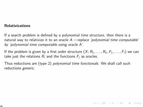
Relativizations

If a search problem is defined by a polynomial time structure, then there is anatural way to relativize it to an oracle A —replace ‘polynomial time computable’by ‘polynomial time computable using oracle A’.

If the problem is given by a first order structure (X ; R1, . . . ,Rk ,F1, . . . ,Fl) we cantake just the relations Ri and the functions Fj as oracles.

Thus reductions are (type 2) polynomial time functionals. We shall call suchreductions generic.

38

To show that such a search problem SA is not solvable in polynomial time forsome oracle A (ie., to show SA 6∈ FPA) is usually easy—by diagonalization.

Theorem (Riis 1993)

Let a search problem S be defined by an existential sentence ∃yφ in the language(R1, . . . ,Rk ,F1, . . . ,Fl) where all Ri and Fj are generic relations and functions(thus we do not allow ≤ etc.).

If ¬∃yφ has an infinite model, then SA 6∈ PLSA,

for some oracle A.

Example. PPPA 6⊆ PLSA

— there exists a model in which PHP fails

39

To show that such a search problem SA is not solvable in polynomial time forsome oracle A (ie., to show SA 6∈ FPA) is usually easy—by diagonalization.

Theorem (Riis 1993)

Let a search problem S be defined by an existential sentence ∃yφ in the language(R1, . . . ,Rk ,F1, . . . ,Fl) where all Ri and Fj are generic relations and functions(thus we do not allow ≤ etc.).

If ¬∃yφ has an infinite model, then SA 6∈ PLSA,

for some oracle A.

Example. PPPA 6⊆ PLSA

— there exists a model in which PHP fails

39

Let Pi , i = 1, 2 be two search problems defined by existential formulas. Let {αn},resp. {βn} be a sequence of propositions (tautologies) expressing the totality ofproblem P1, resp. P2.

Theorem (Buresh-Oppenheim, Morioka)

If there exists a generic reduction of P1 to P2, then tautologies {αn} havepolynomial size bounded depth propositional proofs from tautologies {βn}.

Thus we can show relativized separations by proving lower bounds on the lengthsof propositional proofs.

40

Provably total search problems in theories corresponding to complexityclasses

Theorem (Buss 1986)

FP is exactly the class of search problems provably total in ΘP.

Theorem (Buss, Krajıcek 1994)

PLS is exactly the class of search problems provably total in ΘNP.

Theorem (Krajıcek, Skelley, Thapen 2006)

CPLS is exactly the class of search problems provably total in ΘΣ2 .

More recently, Skelley and Thapen characterized search problems for all ΘΣk .

41


Theorem (Buss 1986)







41


Theorem (Buss 1986)







41

A characterization of provably total search problems of ΘΣ3 .

Let c(p, x , y , z) (cost) and g1(p, x), g2(p, y), g3(p, z) (strategy) be polynomialtime computable functions.Given a, find u, v ,w such that

c(a, u, g2(a, u, v),w) ≥ c(a, g1(a, u), v , g3(a, v ,w)).

Interpretation

- c(p, x , y , z) defines the payoff in a 3-step games parameterized by p;

- two players A and B play two copies of the game;

- B is given by the strategy g1(p, x), g2(p, x , y), g3(p, y , z);

- our goal is to find moves for A such that he gains at least as much in the firstcopy as B gets in the second.

A B → A↓ g1 ↑ g2 ↓ g3

B → A B

42

A B → A : c(u, g2(u, v),w)↓ g1 ↑ g2 ↓ g3 ≥B → A B : c(g1(u), v , g3(v ,w))

LetC := max

xmin

ymax

zc(x , y , z),

then∃x∀y∃z c(x , y , z) ≥ C and ∀x∃y∀z C ≤ c(x , y , z).

Therefore

N |= ∃u∃v∃w c(u, g2(u, v),w) ≥ c(g1(u), v , g3(v ,w)).

But note that finding C is Σp3-hard.

43

Feasible incompleteness

The Feasible Incompleteness Thesis.The phenomenon of incompleteness manifests itself at the level of polynomialtime computations.

1 The feasible consistency problem.

2 Incompleteness caused by complexity.

44

The feasible consistency problem

Assume that all theories are axiomatized by a finite, or polynomial timecomputable set of axioms.

ConT (n) ≡df “there is no T -proof of contradiction of length n.”

Given theories S and T ,

1 do the sentences ConT (n) have S-proofs of length at most p(n) for somepolynomial p?

2 Is there a polynomial time algorithm for finding S-proofs of ConT (n)?

Theorem1. For every consistent and finitely axiomatized theory T , there exists ε > 0 suchthat, for every n, every T -proof of ConT (n) has size at least nε. [Friedman, 1979]2. For every consistent and finitely axiomatized theory T , there exists C suchthat, for every n, there exists T -proof of ConT (n) of size ≤ Cn. [Pudlak, 1984]

45

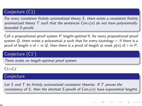
Conjecture (C1)

For every consistent finitely axiomatized theory S, there exists a consistent finitelyaxiomatized theory T such that the sentences ConT (n) do not have polynomiallybounded S-proofs.

Call a propositional proof system P length-optimal if, for every propositional proofsystem Q, there exists a polynomial p such that for every tautology τ , if there is aproof of length n of τ in Q, then there is a proof of length at most p(n) of τ in P.

Conjecture (C1’)

There exists no length-optimal proof system.

C1≡C1’

Conjecture

Let S and T be finitely axiomatized consistent theories. If T proves theconsistency of S, then the shortest S-proofs of ConT (n) have exponential lengths.

46

Incompleteness caused by complexity

Conjecture (C2)

For every finitely axiomatized consistent theory T , there exists a total polynomialsearch problem Q which is strictly stronger than all search problems provablytotal in T .

Conjecture (C2’)

There exists no complete problem among total polynomial search problems, thatis, no problem to which total polynomial search problems are reducible.

C2≡C2’

47

A connection between the two parts of the thesis

Conjecture (C3)

For every consistent finitely axiomatized theory S there exists a consistent finitelyaxiomatized theory T such that S-proofs of sentences ConT (n) cannot beproduced by an algorithm in time p(n), for p a polynomial.

Define that a propositional proof system P is optimal if it polynomially simulatesevery propositional proof system.

Conjecture (C3’)

Optimal propositional proof systems do not exist.

Conjecture (C3”)

For every finitely axiomatized consistent theory T , there exists a propositionalproof system P such that T does not prove the soundness of any formalizationof P.

C3≡C3’≡C3”

48

Documents

An Introduction to Proof Complexity, Part II. · Let TAUT be a set of tautologies. A proof system for TAUT is any polynomial time computable function f that maps the set of all binary