An introduction to multilevel data analyses using HLM 6

Vassilis PavlopoulosUniversity of Athens, Greece

European Association of Social Psychology Summer School, Aug. 23 – Sept. 6, 2010, Aegina, Greece

Acknowledgments

I would like to thank Prof. John Neslek and Prof. Jens Asendorpf for the invaluable insight they offered me in understanding what multilevel analyses is – and what it is not!

The data sets used for example purposes come fromJ. Georgas, J. W. Berry, F. J. R. van de Vijver, Ç. Kağitçibaşi, & Y. H. Poortinga (Eds.), Families across cultures: A 30-nation psychological study. Cambridge, UK: Cambridge University Press.

Presentation outline

Understanding levels of analyses

Advantages of multilevel techniques

When are multilevel techniques appropriate?

Rationale of multilevel modelingThe totally unconditional modelAdding predictors

Relevant issuesVariable centeringModel buildingSample sizes and missing values

Using the HLM software

Once you know hierarchies exist, you see them everywhere (Kreft & de Leeuw, 1998)

Understanding levels of analysis

The term “levels of analysis” refers to how the data isorganized. In statistical terms, the question is whether observations are dependent or not.

When data is hierarchically structured, higher numbers refer to higher levels of hierarchy.

Examples of hierarchically structured data:Persons (L1) nested within groups (L2), e.g. students within classrooms, people within countries.Behaviours (L1) nested within persons (L2), e.g. longitudinal data or diary studies.

Some terminology

The term “Multilevel random coefficient model” (MRCM), sometimes simplified as “multilevel model”, refers to the technique or approach of analyzing hierarchically structured data…

…while the term “Hierarchical Linear Model” (HLM) refers to the program or software used to carry out multilevel analyses (de Leeuw & Kreft, 1995).

Other programs: MlwiN, Mplus, R, etc.

“Ordinary Least Squares” (OLS) refers to traditional techniques, such as ANOVA or regression, that do not distinguish between fixed and random coefficients.

Why HLM? Advantages of MRCM over OLS

In hierarchically structured data, observations at L1 are not independent, which violates a fundamental assumption of OLS approach.

Single-level analyses that ignore the hierarchical structure of the data can provide misleading resultssince relationships at different levels of analyses are independent.

Even when dummy coded variables are used to account for this issue, such analyses still violate important assumptions about sampling error.

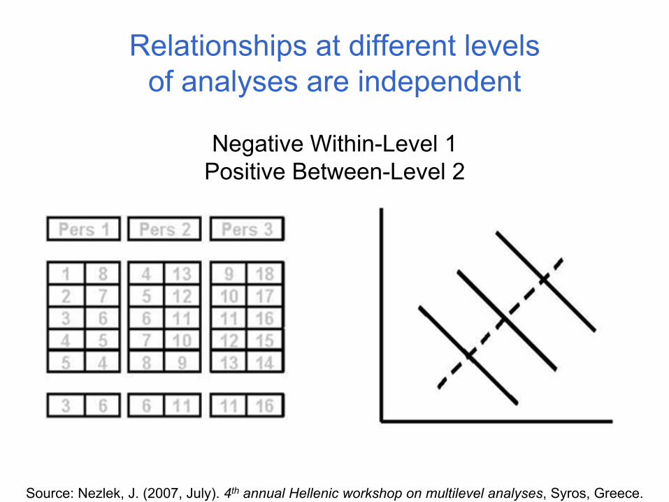
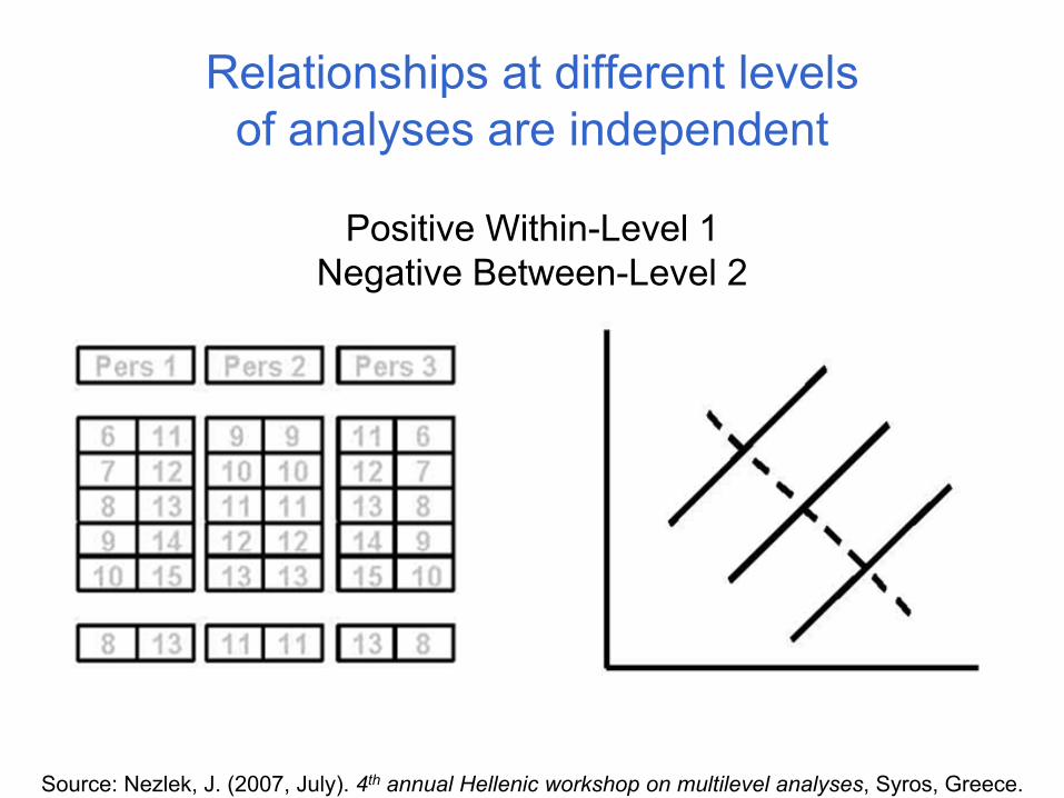
Relationships at different levels of analyses are independent

Source: Nezlek, J. (2007, July). 4th annual Hellenic workshop on multilevel analyses, Syros, Greece.

Negative Within-Level 1Positive Between-Level 2

Relationships at different levels of analyses are independent

Source: Nezlek, J. (2007, July). 4th annual Hellenic workshop on multilevel analyses, Syros, Greece.

Positive Within-Level 1Negative Between-Level 2

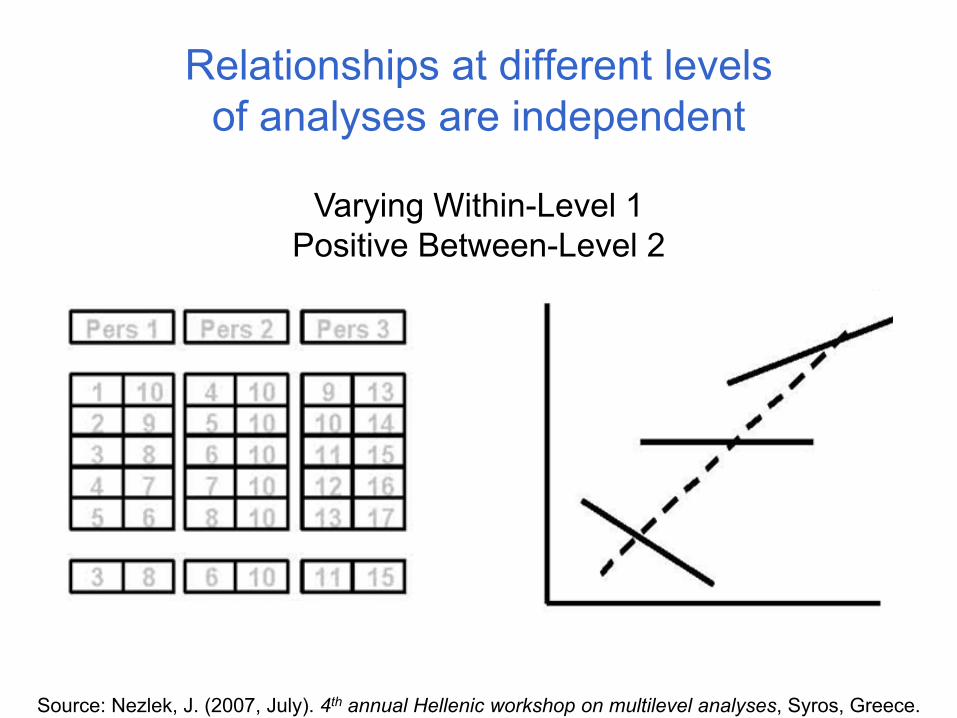
Relationships at different levels of analyses are independent

Source: Nezlek, J. (2007, July). 4th annual Hellenic workshop on multilevel analyses, Syros, Greece.

Varying Within-Level 1Positive Between-Level 2

Why HLM? Advantages of MRCM over OLS

In psychological research, inferences are made for a unit of analysis by studying random samples. MRCMtakes into account simultaneously the sampling error at different levels (not the case in OLS).

MRCM produces more accurate estimates than OLS because it takes into account the reliability of scores and the differences in sample sizes.

The advantages of MRCM are pronounced:when hypotheses of interest concern within-unitrelationships, and when the data structure is irregular, for example due to missing data at L1 (Nezlek, 2008).

When is MRCM appropriate?

Multilevel analyses are appropriate when the data has a multilevel structure.

Many analysts suggest that hierarchies can be ignored if the ICC (which represents the relative distribution of between- and within-group variance) is close to 0.

However, Nezlek (2008) has shown that, even if there is no between-group variance, relationships among variables may still vary across groups.

Restrictions stem from the sample size. More groups with fewer cases are preferable to fewer groups with more cases each (Kreft, 1996, cf. Hofmann, 1997).

What is the rationale of MRCM?

For each level 2 unit, a level 1 model is estimated. These equations are functionally equivalent to a standard OLS regression.

The estimated coefficients then become the dependent measures at the next level of analysis.

For example, in a cross-cultural study for the prediction of family roles (DV) from family values (IV), separate regressions are carried out simultaneously for each participating country (level 2), which then become dependent variables at level 1 (individuals).

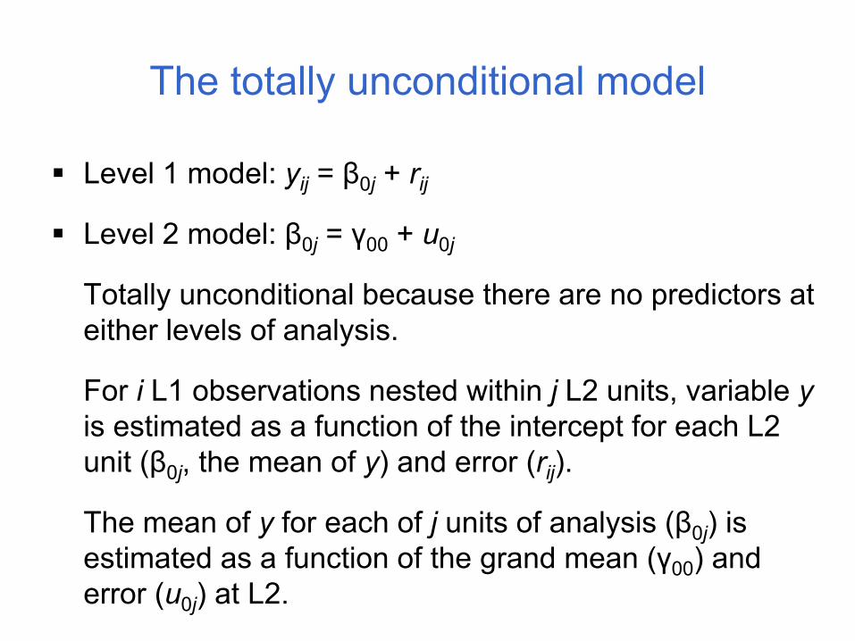
The totally unconditional model

Level 1 model: yij = β0j + rij

Level 2 model: β0j = γ00 + u0j

Totally unconditional because there are no predictors at either levels of analysis.

For i L1 observations nested within j L2 units, variable yis estimated as a function of the intercept for each L2 unit (β0j, the mean of y) and error (rij).

The mean of y for each of j units of analysis (β0j) is estimated as a function of the grand mean (γ00) and error (u0j) at L2.

Adding a predictor at level 2

Level 1 model: yij = β0j + rij

y: Expressive Role of Mother (ERM)

Intercept (β0j): Overall mean of y

Level 2 model: β0j = γ00 + γ01(AFFLUENCE) + u0j

Does the expressive role of mother differ as a function of a country’s affluence index? Such questions involve group mean differences, i.e. intercepts

Adding a predictor at level 1

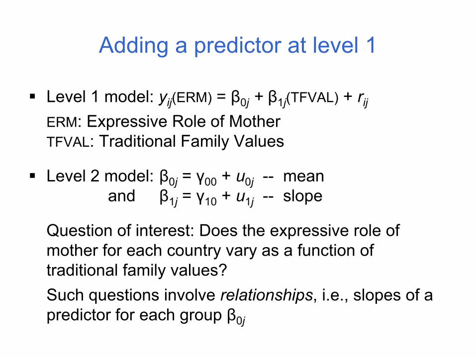
Level 1 model: yij(ERM) = β0j + β1j(TFVAL) + rij

ERM: Expressive Role of MotherTFVAL: Traditional Family Values

Level 2 model: β0j = γ00 + u0j -- meanand β1j = γ10 + u1j -- slope

Question of interest: Does the expressive role of mother for each country vary as a function of traditional family values? Such questions involve relationships, i.e., slopes of a predictor for each group β0j

Adding predictors at levels 1 and 2

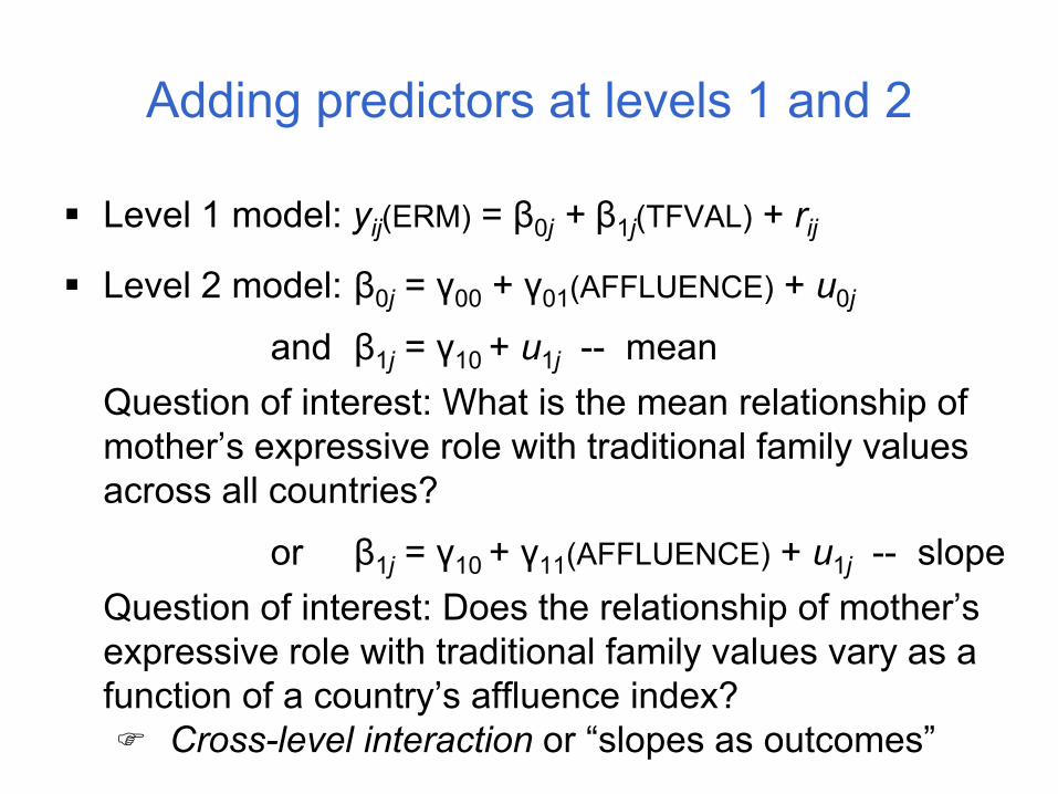
Level 1 model: yij(ERM) = β0j + β1j(TFVAL) + rij

Level 2 model: β0j = γ00 + γ01(AFFLUENCE) + u0j

and β1j = γ10 + u1j -- meanQuestion of interest: What is the mean relationship of mother’s expressive role with traditional family values across all countries?

or β1j = γ10 + γ11(AFFLUENCE) + u1j -- slopeQuestion of interest: Does the relationship of mother’s expressive role with traditional family values vary as a function of a country’s affluence index?

Cross-level interaction or “slopes as outcomes”

Variable centering

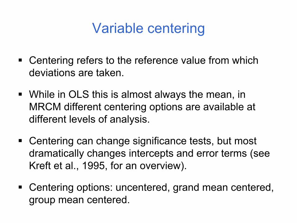
Centering refers to the reference value from which deviations are taken.

While in OLS this is almost always the mean, in MRCM different centering options are available at different levels of analysis.

Centering can change significance tests, but most dramatically changes intercepts and error terms (see Kreft et al., 1995, for an overview).

Centering options: uncentered, grand mean centered, group mean centered.

Variable centering

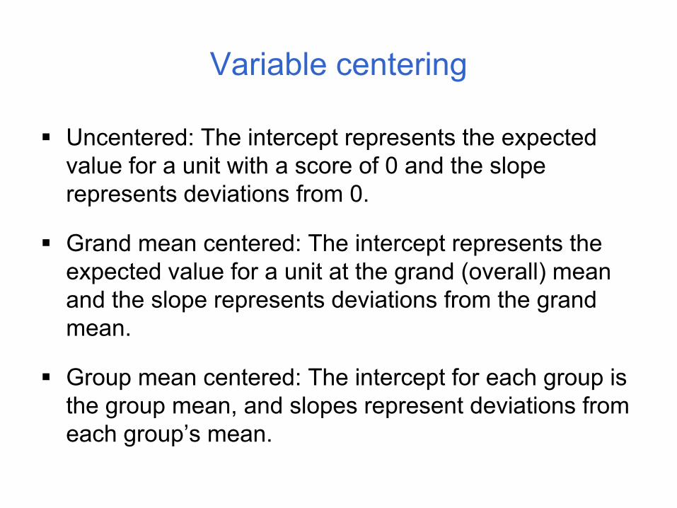
Uncentered: The intercept represents the expected value for a unit with a score of 0 and the slope represents deviations from 0.

Grand mean centered: The intercept represents the expected value for a unit at the grand (overall) meanand the slope represents deviations from the grand mean.

Group mean centered: The intercept for each group is the group mean, and slopes represent deviations from each group’s mean.

Variable centering

With grand mean centering, estimates of slopesinclude between group differences in means ofpredictors. These are not included in group mean centering.

At L2 (in 2-level models), it is recommended to grand mean center, since it helps interpreting the intercept.

At L1, group mean centering is closest to conductingwithin group regression analyses.

Categorical variables are usually uncentered.

Model building

How many levels? Law of parsimony.

Start building a model at level 1, then level 2.

Forward (instead of backward) stepping is generally recommended – add one predictor at a time.

Carrying capacity of data: Larger samples provide more information to estimate parameters.

Modeling error: Determine if effects are fixed or random.

Modeling error variance

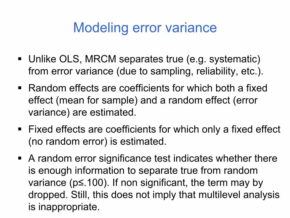
Unlike OLS, MRCM separates true (e.g. systematic) from error variance (due to sampling, reliability, etc.).

Random effects are coefficients for which both a fixed effect (mean for sample) and a random effect (error variance) are estimated.

Fixed effects are coefficients for which only a fixed effect (no random error) is estimated.

A random error significance test indicates whether there is enough information to separate true from random variance (p≤.100). If non significant, the term may by dropped. Still, this does not imply that multilevel analysis is inappropriate.

Sample sizes and missing values

Missing data are not allowed at levels 2 & 3. However, they are allowed at L1 (use option: “delete missing data when running analyses” in HLM).

Check if there is a systematic pattern in missing data.

For predicting any single L2 outcome, the 10-to-1 rule of thumb is recommended (Raudenbush & Bryk, 2002; Raudenbush et al., 2004).

In general, more power is gained for L2 effects by increasing the N of groups (no less than 10-12), whilethe power of L1 effects depends more on the total sample size (Hofmann, 1997).

Using the HLM – Overview

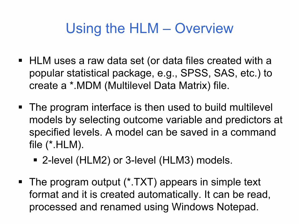
HLM uses a raw data set (or data files created with a popular statistical package, e.g., SPSS, SAS, etc.) to create a *.MDM (Multilevel Data Matrix) file.

The program interface is then used to build multilevel models by selecting outcome variable and predictors at specified levels. A model can be saved in a command file (*.HLM).

2-level (HLM2) or 3-level (HLM3) models.

The program output (*.TXT) appears in simple text format and it is created automatically. It can be read, processed and renamed using Windows Notepad.

Using the HLM – Data preparation

Create a data file for each level of analysis.

Data files need to be sorted in the same order by an ID variable (there is one such ID for 2-level data and two IDs for 3-level data structures). The programme thenuses the ID variable to join the data files.

HLM has no variable transformation capabilities (such as Recode or Compute). It does create cross-level inter-action terms, though within-level interactions should be created in advance. More importantly, it can center variables (around the group mean or the grand mean).

Using the HLM – Creating an MDM file

Select File Make new MDM file Stat package input.

Choose between 2-level HLM2 or 3-level HLM3 models.

In the Make MDM window, select the appropriate Input File Type from the drop-down menu.

Choose between two options of data input nesting: persons within groups or measures within persons(makes no difference in most cases!).

Browse folders to select Level-1 file. Then, choose variables (ID and working variables in MDM).

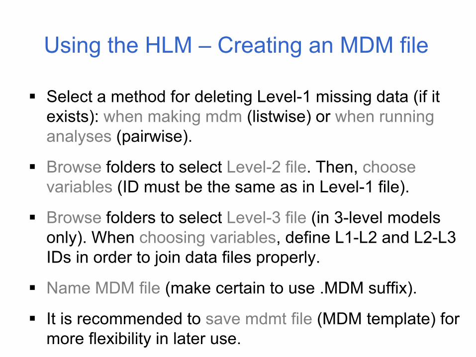
Select a method for deleting Level-1 missing data (if it exists): when making mdm (listwise) or when running analyses (pairwise).

Browse folders to select Level-2 file. Then, choose variables (ID must be the same as in Level-1 file).

Browse folders to select Level-3 file (in 3-level models only). When choosing variables, define L1-L2 and L2-L3 IDs in order to join data files properly.

Name MDM file (make certain to use .MDM suffix).

It is recommended to save mdmt file (MDM template) for more flexibility in later use.

Using the HLM – Creating an MDM file

Select Make MDM

Select Check Stats and review the summary statistics for inconsistencies. The default name for this file is HLM2MDM.STS (recommended to rename and save).

Select Done. Three files have been created so far: The *.mdm file, which will serve as the basis for all multilevel analyses.The *.mdmt file, which is a MDM template. It can be edited through HLM to create new MDM files from the same data set (very convenient!).The HLM2MDM.STS file with summary statistics.

Using the HLM – Creating an MDM file

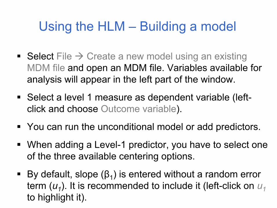
Select File Create a new model using an existing MDM file and open an MDM file. Variables available for analysis will appear in the left part of the window.

Select a level 1 measure as dependent variable (left-click and choose Outcome variable).

You can run the unconditional model or add predictors.

When adding a Level-1 predictor, you have to select one of the three available centering options.

By default, slope (β1) is entered without a random error term (u1). It is recommended to include it (left-click on u1to highlight it).

Using the HLM – Building a model

To add Level-2 predictors, click on the >>Level-2<<button first.

There are two available options for centering Level-2 variables (group-mean centering is makes no sense).

If a L1 measure has already been included, you may wish to specify L2 predictors of both L1 coefficients (intercepts and slopes). Adding a L2 predictor of L1 slope produces a cross-level interaction term.

Save command file (default name is newcmd.hlm –extension .hlm given automatically).

Select Run Analysis to run the model.

Using the HLM – Building a model

Select File View Output. Output file will open in Notepad with default name hlm2.txt (recommended to rename and retain).

First part displays general information, such as number of L1 & L2 units, and equation of the model specified.

Sigma_squared (σ2) refers to L1 variance components.

Tau (Τ) refers to L2 variance-covariance components.

The average Reliability estimates for random L1 coefficients represent the ratio of true variance to the total variance for a parameter. If < 0.100, maybe multivariate analysis is not appropriate.

Using the HLM – Interpretation of output

Usually, research questions refer to significance of fixed effects.

Two tables of fixed effects are produced: the first one based on OLS estimates and the second (with robust standard errors) on maximum likelihood estimates. The latter is recommended to be taken into account.

Significance of a fixed effect: is it different from 0?

It is recommended to estimate predicted values of the DV for +/-1 unit of a continuous predictor in order to appreciate the magnitude of a significant effect.

Using the HLM – Interpretation of output

Error terms from models with an effect and without effect (unconditional) can be compared in order to calculate effect sizes. However, there are limitations on the accuracy of using such variance estimates in HLM (e.g., Hofmann, 1997; Nezlek, 2008).

In what concerns significance tests of random effects (variance components), it is generally preferable to have significant error variance. If not, some analysts suggest that multilevel approach may not be appropriate.

Using the HLM – Interpretation of output

Hofmann, D.A. (1997). An overview of the logic and rationale of hierarchical linear models. Journal of Management, 23(6), 723–744.

Kreft, I.G.G., & de Leeuw, J. (1998). Introducing multilevel modeling. Newbury Park, CA: Sage.

Kreft, I.G.G., de Leeuw, J., & Aiken, L.S. (1995). The effect of different forms of centering in Hierarchical Linear Models. Multivariate Behavioral Research, 30, 1–21.

de Leeuw, J., & Kreft, I.G.G. (1995). Questioning multilevel models. Journal of Educational and Behavioral Statistics, 20,171-189.

References

Nezlek, J. B. (2001). Multilevel random coefficient analyses of event and interval contingent data in Social and Personality Psychology research. Personality and Social Psychology Bulletin, 27, 771–785.

Nezlek, J. N. (2008). An introduction to multilevel modeling for Social and Personality Psychology. Social and Personality Psychology Compass, 2(2), 842–860.

Raudenbush, S.W., & Bryk, A.S. (2002). Hierarchical linear models (2nd ed.). Newbury Park, CA: Sage.

Raudenbush, S.W., Bryk, A.S., Cheong, Y.F., & Congdon, R. (2004). HLM 6: Hierarchical Linear and Nonlinear Modeling. Lincolnwood, IL: Scientific Software International.

References