Embed Size (px)
Citation preview
An Introduction to MDS
FLORIAN WICKELMAIER
Sound Quality Research Unit, Aalborg University, Denmark
May 4, 2003
Author’s note
This manuscript was completed while the author was employed at the Sound Qual-
ity Research Unit at Aalborg University. This unit receives financial support from
Delta Acoustics & Vibration, Bruel & Kjær, and Bang & Olufsen, as well as from
the Danish National Agency for Industry and Trade (EFS) and the Danish Technical
Research Council (STVF). The author would like to thank Karin Zimmer and Wolf-
gang Ellermeier for numerous helpful comments on earlier drafts of the manuscript.
I am also indebted to Jody Ghani for her linguistic revision of the paper. Cor-
respondence concerning this article should be addressed to Florian Wickelmaier,
Department of Acoustics, Aalborg University, Fredrik Bajers Vej 7 B5, 9220 Aal-
borg East, Denmark (email: [email protected]).
1

Abstract
Multidimensional scaling (MDS) is a classical approach to the problem of finding
underlying attributes or dimensions, which influence how subjects evaluate a given
set of objects or stimuli. This paper provides a brief introduction to MDS. Its basic
applications are outlined by several examples. For the interested reader a short
overview of recommended literature is appended. The purpose of this paper is to
facilitate the first contact with MDS to the non-statistician.
2

Contents
Introduction 4
1 Deriving proximities 5
1.1 Direct methods . . . . . . . . . . . . . . . . . . . . . . . . . . . . . . 5
(Dis)Similarity ratings . . . . . . . . . . . . . . . . . . . . . . . . . . 5
Sorting tasks . . . . . . . . . . . . . . . . . . . . . . . . . . . . . . . 6
1.2 Indirect methods . . . . . . . . . . . . . . . . . . . . . . . . . . . . . 6
Confusion Data . . . . . . . . . . . . . . . . . . . . . . . . . . . . . . 6
Correlation matrices . . . . . . . . . . . . . . . . . . . . . . . . . . . 7
2 How does MDS work? 9
2.1 Classical MDS . . . . . . . . . . . . . . . . . . . . . . . . . . . . . . . 9
Steps of a classical MDS algorithm . . . . . . . . . . . . . . . . . . . 10
Example: Cities in Denmark . . . . . . . . . . . . . . . . . . . . . . . 10
2.2 Nonmetric MDS . . . . . . . . . . . . . . . . . . . . . . . . . . . . . . 12
Judging the goodness of fit . . . . . . . . . . . . . . . . . . . . . . . . 13
Basics of a nonmetric MDS algorithm . . . . . . . . . . . . . . . . . . 14
3 Sound quality evaluation using MDS 16
3.1 Individual analysis . . . . . . . . . . . . . . . . . . . . . . . . . . . . 16
3.2 Aggregate analysis . . . . . . . . . . . . . . . . . . . . . . . . . . . . 18
3.3 Individual difference scaling . . . . . . . . . . . . . . . . . . . . . . . 19
Conclusion . . . . . . . . . . . . . . . . . . . . . . . . . . . . . . . . . 20
4 Decisions to take before you start 21
5 MDS literature 24
References 25
List of Figures 26
List of Tables 26
3
Introduction
Multidimensional scaling (MDS) has become more and more popular as a technique
for both multivariate and exploratory data analysis. MDS is a set of data analysis
methods, which allow one to infer the dimensions of the perceptual space of subjects.
The raw data entering into an MDS analysis are typically a measure of the global
similarity or dissimilarity of the stimuli or objects under investigation. The primary
outcome of an MDS analysis is a spatial configuration, in which the objects are
represented as points. The points in this spatial representation are arranged in such
a way, that their distances correspond to the similarities of the objects: similar
object are represented by points that are close to each other, dissimilar objects by
points that are far apart.
This paper is to provide a first introduction to MDS by briefly discussing some
of the issues a researcher is confronted with when applying this method. This
introduction is based mainly on the textbooks of Borg & Groenen (1997), Hair,
Anderson, Tatham & Black (1998), and Cox & Cox (1994), which are also mentioned
in section 5 (MDS literature) of this paper.
The first section covers problems connected with data collection. An overview
of direct and indirect methods of deriving the so-called proximities is given. The
second section may be regarded as a theoretical outline of important MDS methods.
The algorithms of both classical and nonmetric MDS are sketched without going too
deep into the mathematical detail. Section three illustrates different types of MDS
analyses using an example from sound quality evaluation. Section four describes the
many degrees of freedom a researcher has when performing MDS, and provides some
guidelines for choosing the right options. Finally, in the last section, the interested
reader can find recommended MDS literature.
4

1 Deriving proximities
The data for MDS analyses are called proximities. Proximities indicate the overall
similarity or dissimilarity of the objects under investigation. An MDS program looks
for a spatial configuration of the objects, so that the distances between the objects
match their proximities as closely as possible. Often the data are arranged in a
square matrix – the proximity matrix. There are two major groups of methods for
deriving proximities: direct, and indirect methods.
1.1 Direct methods
Subjects might either assign a numerical (dis)similarity value to each pair of ob-
jects, or provide a ranking of the pairs with respect to their (dis)similarity. Both
approaches are direct methods of collecting proximity data.
(Dis)Similarity ratings
Typically, in a rating task subjects are asked to express the dissimilarity of two
objects by a number. Often a 7- or a 9-point scale is used. In the case of a
dissimilarity scale, a low number indicates a strong similarity between two stimuli,
and a high number a strong dissimilarity. In order to obtain the ratings, all possible
pairs of objects have to be presented to the participant (a total number of n(n−1)/2,
where n is the number of objects). This assumes, however, that the dissimilarity
relation is symmetrical, and thus the order within each pair is of no relevance.
Many MDS programs can also handle asymmetric proximity data, where for example
object a is more similar to object b than b to a. Asymmetric proximities might for
example arise when collecting confusion data (see below). Investigating asymmetric
proximity relations, however, doubles the number of pairs to be presented.
The advantage of direct ratings is that the data are immediately ready for an
MDS analysis. Therefore, both an individual investigation of each participant, and
an aggregate analysis based on averages across the proximity matrices are possible.
A disadvantage of dissimilarity ratings is the rapidly growing number of paired
comparisons, as the number of objects increases.
5

Sorting tasks
There are many ways of asking subjects for the order of the similarities. One option
is to write each object pair on a card and let the participant sort the cards from
the lowest similarity to the highest. Another method is to let the subject put cards
with pairs of low similarity into one pile, cards with pairs of higher similarity in the
next pile and so on. Afterwards, a numerical value of (dis)similarity is assigned to
each pile. Yet another approach is to write only one object on each card and ask
the participants to sort the cards with the most similar objects into piles. Counting
how many times two objects appear together in a pile, yields the similarity matrix.
The advantage of the sorting methods is that they are very intuitive for subjects,
but some of them do not allow for an individual analysis of the data.
1.2 Indirect methods
Indirect methods for proximity data do not require that a subject assigns a numer-
ical value to the elements of the proximity matrix directly. Rather, the proximity
matrix is derived from other measures, e. g. from confusion data or from correlation
matrices.
Confusion Data
Confusion data arise when the researcher records how often subjects mistake one
stimulus for another. Consider an experiment where the letters of the alphabet are
briefly presented via loudspeaker. The task of the subject is to recognize the letter.
From the data a proximity matrix can be derived: letters that are rarely confused
get a high dissimilarity value, letters that are often confused a low one.
An advantage of using confusion data is that the similarity of stimuli is judged
on a perceptual level without involving much cognitive processing. Thus, very basic
perceptual dimensions might be revealed using this technique. On the other hand,
confusion data are often asymmetric and do not allow for an individual analysis.
Most notably, there must be a good chance of confusing one object with the other,
which excludes perfectly discriminable stimuli from being investigated using this
method.
6
crime no. 1 2 3 4 5 6 7
murder 1 1.00 0.52 0.34 0.81 0.28 0.06 0.11
rape 2 0.52 1.00 0.55 0.70 0.68 0.60 0.44
robbery 3 0.34 0.55 1.00 0.56 0.62 0.44 0.62
assault 4 0.81 0.70 0.56 1.00 0.52 0.32 0.33
burglary 5 0.28 0.68 0.62 0.52 1.00 0.80 0.70
larceny 6 0.06 0.60 0.44 0.32 0.80 1.00 0.55
auto theft 7 0.11 0.44 0.62 0.33 0.70 0.55 1.00
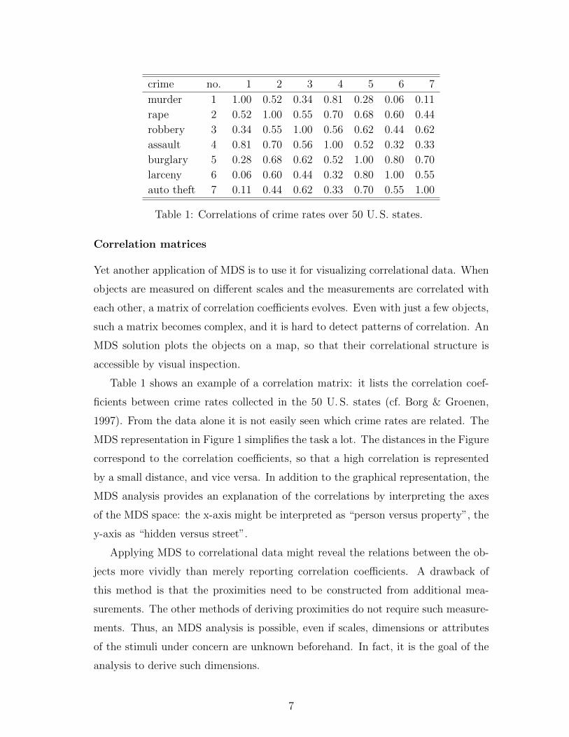
Table 1: Correlations of crime rates over 50 U. S. states.
Correlation matrices
Yet another application of MDS is to use it for visualizing correlational data. When
objects are measured on different scales and the measurements are correlated with
each other, a matrix of correlation coefficients evolves. Even with just a few objects,
such a matrix becomes complex, and it is hard to detect patterns of correlation. An
MDS solution plots the objects on a map, so that their correlational structure is
accessible by visual inspection.
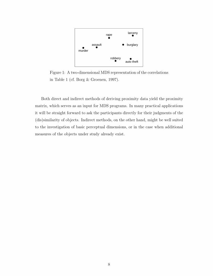
Table 1 shows an example of a correlation matrix: it lists the correlation coef-
ficients between crime rates collected in the 50 U. S. states (cf. Borg & Groenen,
1997). From the data alone it is not easily seen which crime rates are related. The
MDS representation in Figure 1 simplifies the task a lot. The distances in the Figure
correspond to the correlation coefficients, so that a high correlation is represented
by a small distance, and vice versa. In addition to the graphical representation, the
MDS analysis provides an explanation of the correlations by interpreting the axes
of the MDS space: the x-axis might be interpreted as “person versus property”, the
y-axis as “hidden versus street”.
Applying MDS to correlational data might reveal the relations between the ob-
jects more vividly than merely reporting correlation coefficients. A drawback of
this method is that the proximities need to be constructed from additional mea-
surements. The other methods of deriving proximities do not require such measure-
ments. Thus, an MDS analysis is possible, even if scales, dimensions or attributes
of the stimuli under concern are unknown beforehand. In fact, it is the goal of the
analysis to derive such dimensions.
7
murder
rape
robbery
assault burglary
larceny
auto theft
Figure 1: A two-dimensional MDS representation of the correlations
in Table 1 (cf. Borg & Groenen, 1997).
Both direct and indirect methods of deriving proximity data yield the proximity
matrix, which serves as an input for MDS programs. In many practical applications
it will be straight forward to ask the participants directly for their judgments of the
(dis)similarity of objects. Indirect methods, on the other hand, might be well suited
to the investigation of basic perceptual dimensions, or in the case when additional
measures of the objects under study already exist.
8
2 How does MDS work?
The goal of an MDS analysis is to find a spatial configuration of objects when all that
is known is some measure of their general (dis)similarity. The spatial configuration
should provide some insight into how the subject(s) evaluate the stimuli in terms
of a (small) number of potentially unknown dimensions. Once the proximities are
derived (cf. section 1) the data collection is concluded, and the MDS solution has
to be determined using a computer program.
Many MDS programs make a distinction between classical and nonmetric MDS.
Classical MDS assumes that the data, the proximity matrix, say, display metric
properties, like distances as measured from a map. Thus, the distances in a classical
MDS space preserve the intervals and ratios between the proximities as good as
possible. For a data matrix consisting of human dissimilarity ratings such a metric
assumption will often be too strong. Nonmetric MDS therefore only assumes that
the order of the proximities is meaningful. The order of the distances in a nonmetric
MDS configuration reflects the order of the proximities as good as possible while
interval and ratio information is of no relevance.
In order to gain a better understanding of the MDS outcome, a brief introduction
to the basic mechanisms of the two MDS procedures, classical und nonmetric MDS,
might be helpful.
2.1 Classical MDS
Consider the following problem: looking at a map showing a number of cities, one
is interested in the distances between them. These distances are easily obtained by
measuring them using a ruler. Apart from that, a mathematical solution is available:
knowing the coordinates x and y, the Euclidean distance between two cities a and
b is defined by
dab =√
(xa − xb)2 + (ya − yb)2. (1)
Now consider the inverse problem: having only the distances, is it possible to obtain
the map? Classical MDS, which was first introduced by Torgerson (1952), addresses
this problem. It assumes the distances to be Euclidean. Euclidean distances are
usually the first choice for an MDS space. There exist, however, a number of non-
9
Euclidean distance measures, which are limited to very specific research questions
(cf. Borg & Groenen, 1997). In many applications of MDS the data are not distances
as measured from a map, but rather proximity data. When applying classical MDS
to proximities it is assumed that the proximities behave like real measured distances.
This might hold e. g. for data that are derived from correlation matrices, but rarely
for direct dissimilarity ratings. The advantage of classical MDS is that it provides
an analytical solution, requiring no iterative procedures.
Steps of a classical MDS algorithm
Classical MDS algorithms typically involve some linear algebra. Readers who are
not familiar with these concepts might as well skip the next paragraph (cf. Borg &
Groenen, 1997, for a more careful introduction).
The classical MDS algorithm rests on the fact that the coordinate matrix X can
be derived by eigenvalue decomposition from the scalar product matrix B = XX′.
The problem of constructing B from the proximity matrix P is solved by multiplying
the squared proximities with the matrix J = I − n−111′. This procedure is called
double centering. The following steps summarize the algorithm of classical MDS:
1. Set up the matrix of squared proximities P(2) = [p2].
2. Apply the double centering: B = −12JP(2)J using the matrix J = I− n−111′,
where n is the number of objects.
3. Extract the m largest positive eigenvalues λ1 . . . λm of B and the corresponding
m eigenvectors e1 . . . em.
4. A m-dimensional spatial configuration of the n objects is derived from the
coordinate matrix X = EmΛ1/2m , where Em is the matrix of m eigenvectors
and Λm is the diagonal matrix of m eigenvalues of B, respectively.
Example: Cities in Denmark
In order to illustrate classical MDS, assume that we have measured the distances
between København (cph), Arhus (aar), Odense (ode) and Aalborg (aal) on a map.
10

Therefore, the proximity matrix (showing the distances in millimeters) might look
likecph aar ode aal
cph 0 93 82 133
aar 93 0 52 60
ode 82 52 0 111
aal 133 60 111 0
.
The matrix of squared proximities is
P(2) =
0 8649 6724 17689
8649 0 2704 3600
6724 2704 0 12321
17689 3600 12321 0
.Since there are n = 4 objects, the matrix J is calculated by
J =
1 0 0 0
0 1 0 0
0 0 1 0
0 0 0 1
−0.25×
1 1 1 1
1 1 1 1
1 1 1 1
1 1 1 1
=
0.75 −0.25 −0.25 −0.25
−0.25 0.75 −0.25 −0.25
−0.25 −0.25 0.75 −0.25
−0.25 −0.25 −0.25 0.75
.Applying J to P(2) yields the double centered matrix B
B = −12JP(2)J =
5035.0625 −1553.0625 258.9375 −3740.938
−1553.0625 507.8125 5.3125 1039.938
258.9375 5.3125 2206.8125 −2471.062
−3740.9375 1039.9375 −2471.0625 5172.062
.For a two-dimensional representation of the four cities, the first two largest eigen-
values and the corresponding eigenvectors of B have to be extracted
λ1 = 9724.168, λ2 = 3160.986, e1 =
−0.637
0.187
−0.253
0.704
, e2 =
−0.586
0.214
0.706
−0.334
.
Finally the coordinates of the cities (up to rotations and reflections) are obtained
by multiplying eigenvalues and -vectors
X =
−0.637 −0.586
0.187 0.214
−0.253 0.706
0.704 −0.334
[ √
9724.168 0
0√
3160.986
]=
−62.831 −32.97448
18.403 12.02697
−24.960 39.71091
69.388 −18.76340
.11
−60 −40 −20 0 20 40 60
−40
−20
0
20
40cph
aar
ode
aal
MDS map
Dimension 1
Dim
ensi
on 2
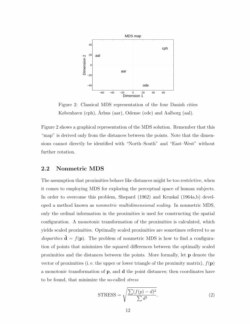
Figure 2: Classical MDS representation of the four Danish cities
København (cph), Arhus (aar), Odense (ode) and Aalborg (aal).
Figure 2 shows a graphical representation of the MDS solution. Remember that this
“map” is derived only from the distances between the points. Note that the dimen-
sions cannot directly be identified with “North–South” and “East–West” without
further rotation.
2.2 Nonmetric MDS
The assumption that proximities behave like distances might be too restrictive, when
it comes to employing MDS for exploring the perceptual space of human subjects.
In order to overcome this problem, Shepard (1962) and Kruskal (1964a,b) devel-
oped a method known as nonmetric multidimensional scaling. In nonmetric MDS,
only the ordinal information in the proximities is used for constructing the spatial
configuration. A monotonic transformation of the proximities is calculated, which
yields scaled proximities. Optimally scaled proximities are sometimes referred to as
disparities d = f(p). The problem of nonmetric MDS is how to find a configura-
tion of points that minimizes the squared differences between the optimally scaled
proximities and the distances between the points. More formally, let p denote the
vector of proximities (i. e. the upper or lower triangle of the proximity matrix), f(p)
a monotonic transformation of p, and d the point distances; then coordinates have
to be found, that minimize the so-called stress
STRESS =
√∑(f(p)− d)2∑
d2. (2)
12
MDS programs automatically minimize stress in order to obtain the MDS solution;
there exist, however, many (slightly) different versions of stress.
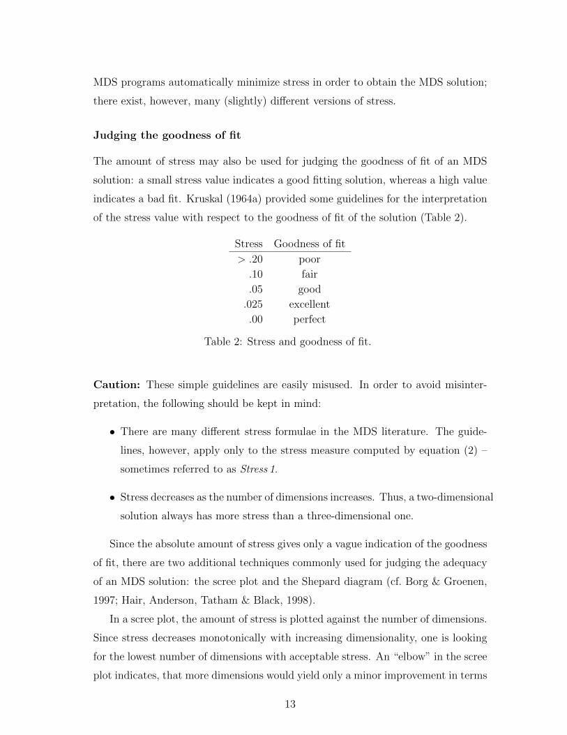
Judging the goodness of fit
The amount of stress may also be used for judging the goodness of fit of an MDS
solution: a small stress value indicates a good fitting solution, whereas a high value
indicates a bad fit. Kruskal (1964a) provided some guidelines for the interpretation
of the stress value with respect to the goodness of fit of the solution (Table 2).
Stress Goodness of fit
> .20 poor
.10 fair
.05 good
.025 excellent
.00 perfect
Table 2: Stress and goodness of fit.
Caution: These simple guidelines are easily misused. In order to avoid misinter-
pretation, the following should be kept in mind:
• There are many different stress formulae in the MDS literature. The guide-
lines, however, apply only to the stress measure computed by equation (2) –
sometimes referred to as Stress 1.
• Stress decreases as the number of dimensions increases. Thus, a two-dimensional
solution always has more stress than a three-dimensional one.
Since the absolute amount of stress gives only a vague indication of the goodness
of fit, there are two additional techniques commonly used for judging the adequacy
of an MDS solution: the scree plot and the Shepard diagram (cf. Borg & Groenen,
1997; Hair, Anderson, Tatham & Black, 1998).
In a scree plot, the amount of stress is plotted against the number of dimensions.
Since stress decreases monotonically with increasing dimensionality, one is looking
for the lowest number of dimensions with acceptable stress. An “elbow” in the scree
plot indicates, that more dimensions would yield only a minor improvement in terms
13
1 2 3 4 50
0.1
0.2
0.3Scree plot
Dimensions
Str
ess
3 4 5 6 7 81
2
3
4
5
6
7
8
9Shepard diagram
Proximities
Dis
tanc
es/D
ispa
ritie
s
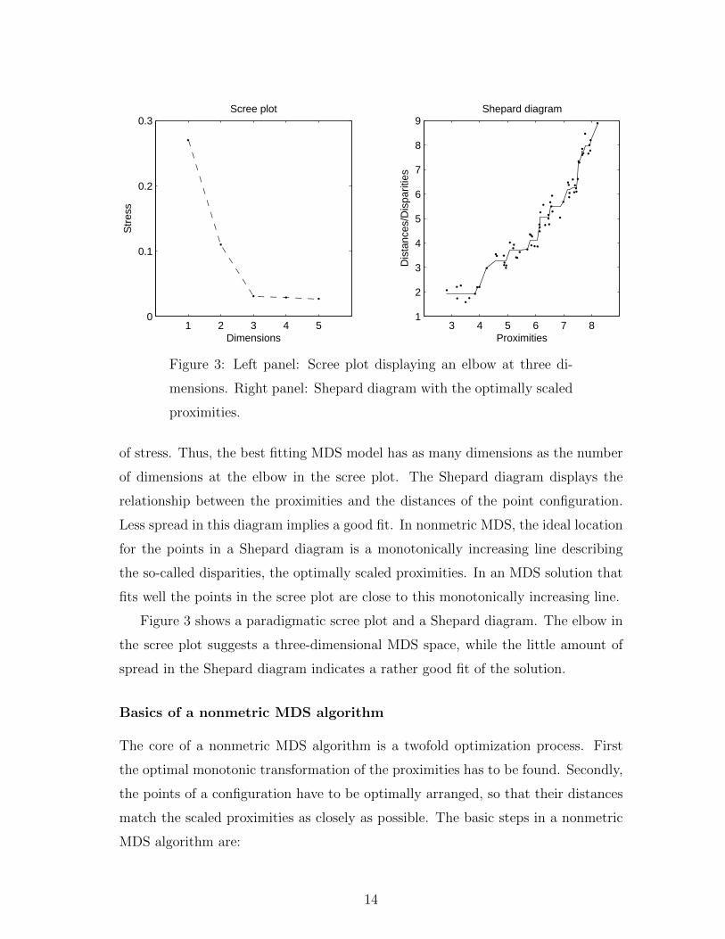
Figure 3: Left panel: Scree plot displaying an elbow at three di-
mensions. Right panel: Shepard diagram with the optimally scaled
proximities.
of stress. Thus, the best fitting MDS model has as many dimensions as the number
of dimensions at the elbow in the scree plot. The Shepard diagram displays the
relationship between the proximities and the distances of the point configuration.
Less spread in this diagram implies a good fit. In nonmetric MDS, the ideal location
for the points in a Shepard diagram is a monotonically increasing line describing
the so-called disparities, the optimally scaled proximities. In an MDS solution that
fits well the points in the scree plot are close to this monotonically increasing line.
Figure 3 shows a paradigmatic scree plot and a Shepard diagram. The elbow in
the scree plot suggests a three-dimensional MDS space, while the little amount of
spread in the Shepard diagram indicates a rather good fit of the solution.
Basics of a nonmetric MDS algorithm
The core of a nonmetric MDS algorithm is a twofold optimization process. First
the optimal monotonic transformation of the proximities has to be found. Secondly,
the points of a configuration have to be optimally arranged, so that their distances
match the scaled proximities as closely as possible. The basic steps in a nonmetric
MDS algorithm are:
14

1. Find a random configuration of points, e. g. by sampling from a normal distri-
bution.
2. Calculate the distances d between the points.
3. Find the optimal monotonic transformation of the proximities, in order to
obtain optimally scaled data f(p).
4. Minimize the stress between the optimally scaled data and the distances by
finding a new configuration of points.
5. Compare the stress to some criterion. If the stress is small enough then exit
the algorithm else return to 2.
15
3 Sound quality evaluation using MDS
The following section gives an example of an application of different types of MDS
analyses in sound quality research. The data were collected at the Sound Quality
Research Unit (SQRU), Aalborg University, in the summer of 2002 by Christian
Schmid. One goal of the study was to reveal and identify the dimensions that
subjects use in evaluating environmental sounds. A total number of 77 subjects
participated in the experiment. They were presented with all 66 pairs of 12 environ-
mental sounds via headphones. The subjects’ task was to rate the dissimilarity of
each two sounds on a scale from 1 (very similar) to 9 (very dissimilar). The resulting
proximity matrices allow for both an individual and an aggregate analysis.
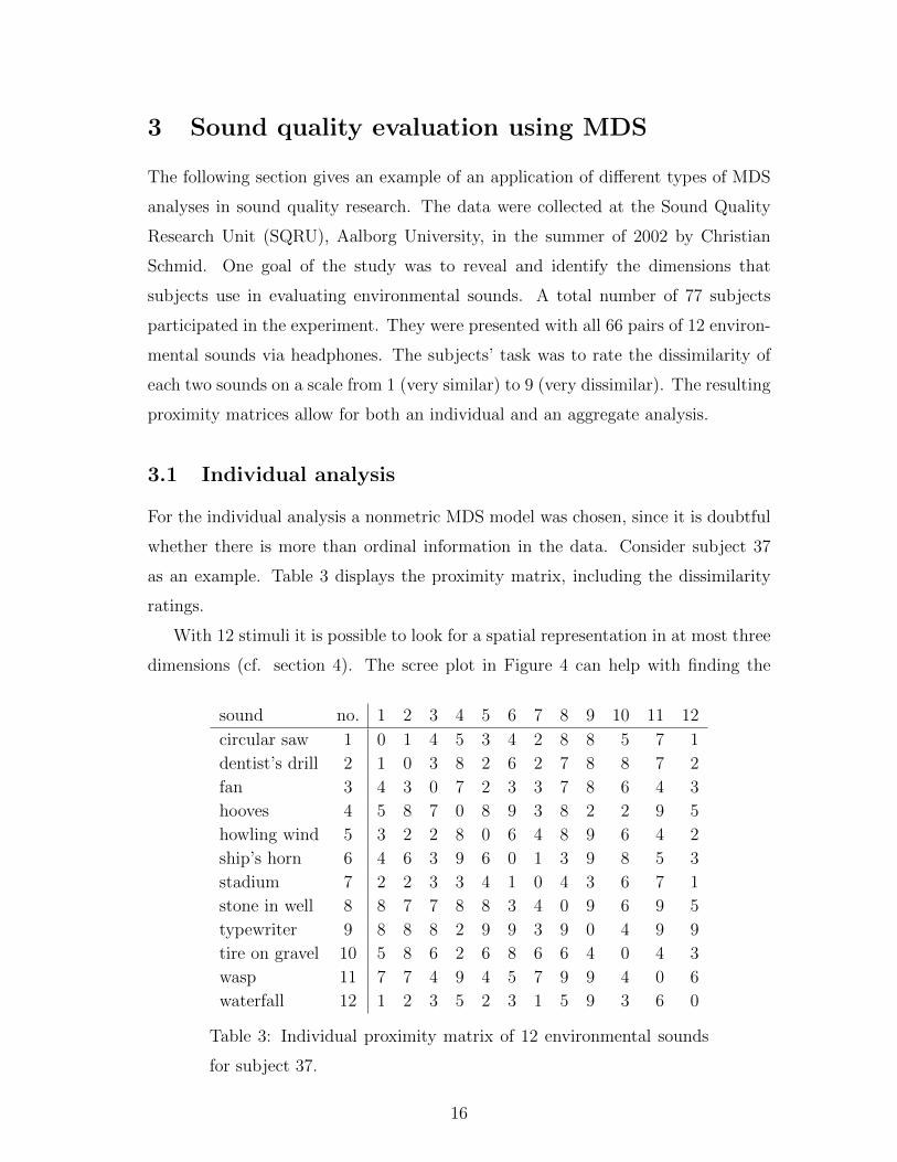
3.1 Individual analysis
For the individual analysis a nonmetric MDS model was chosen, since it is doubtful
whether there is more than ordinal information in the data. Consider subject 37
as an example. Table 3 displays the proximity matrix, including the dissimilarity
ratings.
With 12 stimuli it is possible to look for a spatial representation in at most three
dimensions (cf. section 4). The scree plot in Figure 4 can help with finding the
sound no. 1 2 3 4 5 6 7 8 9 10 11 12
circular saw 1 0 1 4 5 3 4 2 8 8 5 7 1
dentist’s drill 2 1 0 3 8 2 6 2 7 8 8 7 2
fan 3 4 3 0 7 2 3 3 7 8 6 4 3
hooves 4 5 8 7 0 8 9 3 8 2 2 9 5
howling wind 5 3 2 2 8 0 6 4 8 9 6 4 2
ship’s horn 6 4 6 3 9 6 0 1 3 9 8 5 3
stadium 7 2 2 3 3 4 1 0 4 3 6 7 1
stone in well 8 8 7 7 8 8 3 4 0 9 6 9 5
typewriter 9 8 8 8 2 9 9 3 9 0 4 9 9
tire on gravel 10 5 8 6 2 6 8 6 6 4 0 4 3
wasp 11 7 7 4 9 4 5 7 9 9 4 0 6
waterfall 12 1 2 3 5 2 3 1 5 9 3 6 0
Table 3: Individual proximity matrix of 12 environmental sounds
for subject 37.
16

1 2 30
0.1
0.2
0.3
0.4Scree plot
Dimensions
Str
ess
1 2 3 4 5 6 7 8 90
2
4
6
8
10
12Shepard diagram
Proximities
Dis
tanc
es/D
ispa
ritie
s
Figure 4: Scree plot and Shepard diagram for the two-dimensional
MDS solution (subject 37).
appropriate number of dimensions. Obviously, a one-dimensional representation is
not adequate (stress > .30). The scree plot does not display a clear elbow, but
the largest improvement in terms of stress occurs when changing from one to two
dimensions. Therefore, a two-dimensional solution was chosen. The stress for the
two-dimensional solution is 0.156. The Shepard diagram displays the goodness of fit
of the two-dimensional solution. The points of a perfectly fitting solution would lie
on the monotonically increasing line. The spread in the Shepard diagram indicates
some deviation from a perfect fit; it was, however, considered small enough to carry
out further analyses.
In Figure 5 the two-dimensional graphical representation of the proximities of
subject 37 is shown. When interpreting such an MDS map one strategy is to look
for groups of objects. The three objects ‘typewriter’, ‘tire on gravel’, and ‘howling
wind’ for example seem to form a group, since they are closer to each other than
to any other sound. Another approach is to take two very distant objects and try
to find an interpretation for the dimensions. The sounds ‘stone in well’ and ‘wasp’
seem to be very different on dimension two, but rather similar on dimension one.
The substantial interpretation of these dimensions, however, is not obvious.
17

csddfa ho
hw
sh
st
sw
ty
tg
wa
wf
Figure 5: Individual MDS representation (subject 37) of twelve
environmental sounds: circular saw (cs), dentist’s drill (dd), fan
(fa), hooves (ho), howling wind (hw), ship’s horn (sh), stadium
(st), stone in well (sw), typewriter (ty), tire on gravel (tg), wasp
(wa), waterfall (wf).
3.2 Aggregate analysis
In order to perform an aggregate MDS analysis, the 77 single proximity matrices
were combined by computing the average value for each cell. Again, a nonmetric
MDS model with Euclidean distances was chosen to represent the data. The stress
for a two-dimensional solution amounts to 0.106; the largest improvement in terms
of stress occurs when changing from one to two dimensions. The graphical configu-
ration is displayed in Figure 6.
If there are additional measurements of the stimuli available, it is possible to
search for an empirical interpretation of the dimensions by correlating them with
the external measure. In our case, from another experiment with the same sounds
and largely the same subjects, an unpleasantness scale was derived. I. e. the un-
pleasantness value for each sound is known. Correlating the values on the first
dimension (x-axis) with the unpleasantness scale using Spearman’s rank correlation
yields a statistically significant correlation of % = 0.69. Roughly speaking, half of
the variance along the x-axis in Figure 6 can be explained by the unpleasantness of
the sounds. This finding emphasizes the importance of a psychological measure like
unpleasantness for the perception of environmental sounds.
18

csdd
fahohw
sh st
sw
ty
tg
wa
wf
Figure 6: Aggregate MDS representation of twelve environmental
sounds for 77 subjects (the labels of the sounds are the same as in
Figure 5).
3.3 Individual difference scaling
Individual difference scaling (INDSCAL), or weighted MDS, was first introduced
by Carrol & Chang (1970). Using this technique, it is possible to represent both
the stimuli in a common MDS space, and the individual differences. In order to
achieve this, the assumption is made that all subjects use the same dimensions
when evaluating the objects, but that they might apply individual weights to these
dimensions. By estimating the individual weights and plotting them (in the case of
a low-dimensional solution) different groups of subjects can be detected. The input
of an INDSCAL analysis are the individual proximity matrices of all subjects.
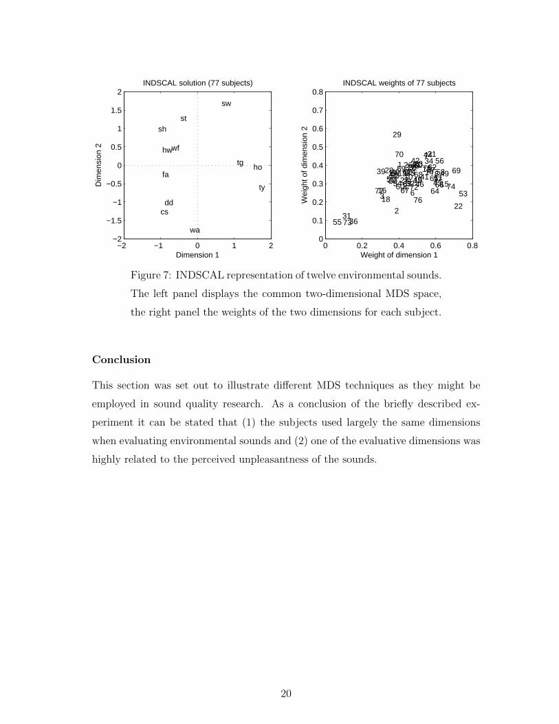
Figure 7 shows the outcome of the INDSCAL procedure as applied to the twelve
environmental sounds and the sample of 77 participants presented in the previous
section. The MDS map looks similar to the aggregate MDS representation depicted
in Figure 6. The tight clustering of the subjects’ weights in the right panel of
Figure 7 reveals that the sample is rather homogeneous. Only the subjects 31, 36,
55, and 73 in the lower left corner of the figure may be regarded as a separate group;
i. e. these participants put less weight on the two dimensions than the rest of the
sample.
19
−2 −1 0 1 2−2
−1.5
−1
−0.5
0
0.5
1
1.5
2
csdd
faho
hw
shst
sw
ty
tg
wa
wf
INDSCAL solution (77 subjects)
Dimension 1
Dim
ensi
on 2
0 0.2 0.4 0.6 0.80
0.1
0.2
0.3
0.4
0.5
0.6
0.7
0.8
1
2
34
5
6
7
8910 111213 14
1516
17
18
1920
21
22
232425
26
2728
29
30
31
32
3334
35
36
373839 40
41
42
43
44
4546
4748
495051
52
5354
55
56575859
60
6162
6364
6566
67
68 69
7071
72
73
74
75
7677
INDSCAL weights of 77 subjects
Weight of dimension 1
Wei
ght o
f dim
ensi
on 2
Figure 7: INDSCAL representation of twelve environmental sounds.
The left panel displays the common two-dimensional MDS space,
the right panel the weights of the two dimensions for each subject.
Conclusion
This section was set out to illustrate different MDS techniques as they might be
employed in sound quality research. As a conclusion of the briefly described ex-
periment it can be stated that (1) the subjects used largely the same dimensions
when evaluating environmental sounds and (2) one of the evaluative dimensions was
highly related to the perceived unpleasantness of the sounds.
20

4 Decisions to take before you start
MDS requires a certain amount of expertise on the part of the researcher. Unlike
univariate statistical methods, the outcome of an MDS analysis is more dependent
on the decisions that are taken beforehand. At the data-collection stage one should
be aware that asking for similarity rather than for dissimilarity ratings might affect
the results; i. e. a similarity judgment cannot simply be regarded as the “inverse” of
a dissimilarity judgment. Further, a decision between direct and indirect methods,
and symmetric versus asymmetric methods of data collection, respectively, has to
be taken (cf. section 1).
The way the proximity matrix has been set up might already determine the
choice of an appropriate MDS model. If the proximities are such that the actual
numerical values are of little significance and the rank order is thought to be the
only relevant information, then a nonmetric, rather than a metric, model should
be chosen. Moreover, Euclidean distances are recommended whenever the most
important goal of the analysis is to visualize the structure in the data; non-Euclidean
distances will rather obscure the outcome from visual inspection, but they might be
a valuable tool for investigating specific hypotheses about the subject’s perceptual
space. Finally, the type of stress measure chosen will affect the MDS representation.
Clearly, the number of dimensions of the MDS space will influence the solution
most drastically. A-priori hypotheses might help to choose the appropriate number.
If, for example, the question is whether or not it is possible to represent the objects
by a unidimensional scale, one will be most interested in a one-dimensional MDS
solution. The number of objects to be scaled gives further guidelines (Borg &
Groenen, 1997): a k-dimensional representation requires at least 4k objects, i. e.
a two-dimensional representation requires at least eight objects. A posteriori, the
amount of stress and the number of interpretable dimensions will provide additional
information on how many dimensions to choose.
Another important decision is the type of MDS analysis to be performed. Again
the specific research question might determine the choice. An individual analysis
represents the data of each subject most accurately. But often one is not interested
in the individual differences, but in the perceptual space of an “average” subject.
In this case, the aggregate analysis is more appropriate. INDSCAL provides both
21
III. Dimensions− 1,2,3 or more dimensions− number of objects
IV. Analysis− individual analysis− aggregate analysis− weighted analysis
V. Software
I. Proximities− similarities vs. dissimilarities− direct vs. indirect methods− symmetric vs. asymmetric data
II. MDS model− metric vs. nonmetric− Euclidean vs. non−Euclidean− type of stress
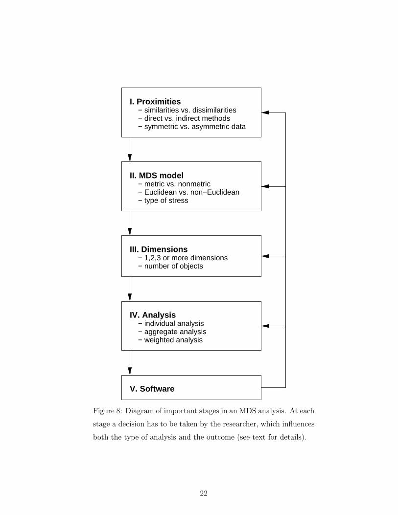
Figure 8: Diagram of important stages in an MDS analysis. At each
stage a decision has to be taken by the researcher, which influences
both the type of analysis and the outcome (see text for details).
22

a common MDS space and a representation of the individual differences. In that
case, however, the assumption is made, that all subjects share a common perceptual
space and differ only in their weights of the dimensions.
Finally, adequate MDS software has to be found that can do the analysis. All
major statistical packages like SPSS, SAS, Statistica, and S-Plus, can perform MDS
analyses. Aside from that stand-alone software exists, specially designed for MDS.
One of the currently most used is ALSCAL by Forrest Young. It is freely available
at http://forrest.psych.unc.edu/research/alscal.html.
However, with the choice of the software, some of the decisions at earlier stages
might be predetermined, e. g. the type of stress measure or the type of analysis.
When buying or using MDS software, one should re-assure that it can perform not
only classical, but also nonmetric MDS. This holds for any of the above-mentioned
software. Figure 8 shows the stages before an MDS analysis and some of the options
the researcher has to choose among.
23

5 MDS literature
Multidimensional scaling now belongs to the standard techniques in statistics, even
though it is rarely treated in introductory textbooks. Specific textbooks on multi-
variate data analysis cover topics in greater detail which are only briefly discussed
in this paper. The following three books I found especially useful in gaining a basic
understanding of MDS.
• Borg & Groenen (1997) provide a thorough introduction to multidimensional
scaling. Features of MDS algorithms are outlined by many examples. Recom-
mended to those who want to know more about what the computer programs
actually do.
• An easy to read, application-oriented overview of MDS is given by Hair, An-
derson, Tatham & Black (1998). This book covers many multivariate analysis
techniques from the economist’s point of view. Highly recommended to the
reader with only basic statistical knowledge.
• Further information on the algorithm for individual difference scaling (IND-
SCAL) as well as on the ALSCAL algorithm can be found in Cox & Cox
(1994). The theoretical results are illustrated by several examples.
24

References
Borg, I., & Groenen, P. (1997). Modern multidimensional scaling: theory and appli-
cations. New York: Springer.
Carrol, J. D., & Chang, J. J. (1970). Analysis of individual differences in multidi-
mensional scaling via an N-way generalization of Echart-Young decomposition.
Psychometrika, 35, 283-319.
Cox, T. F., & Cox, M. A. A. (1994). Multidimensional Scaling. London: Chapman
& Hall.
Hair, J. F., Anderson, T. E., Tatham, R. L., & Black, W. C. (1998). Multivariate
data analysis. Upper Saddle River, NJ: Prentice Hall.
Kruskal, J. B. (1964a). Multidimensional scaling by optimizing goodness of fit to a
nonmetric hypothesis. Psychometrika, 29, 1-27.
Kruskal, J. B. (1964b). Nonmetric multidimensional scaling: a numerical method.
Psychometrika, 29, 115-129.
Shepard, R. N. (1962). The analysis of proximities: multidimensional scaling with
an unknown distance function. Psychometrika, 27, 125-139; 219-246.
Torgerson, W. S. (1952). Multidimensional scaling: I. Theory and method. Psy-
chometrika, 17, 401-419.
25

List of Figures
1 MDS representation of the of the correlations in Table 1 . . . . . . . 8
2 Classical MDS representation of four Danish cities . . . . . . . . . . . 12
3 Scree plot and Shepard diagram . . . . . . . . . . . . . . . . . . . . . 14
4 Scree plot and Shepard diagram for the two-dimensional MDS solution 17
5 Individual MDS representation (subject 37) of twelve environmental
sounds . . . . . . . . . . . . . . . . . . . . . . . . . . . . . . . . . . . 18
6 Aggregate MDS representation of twelve environmental sounds for 77
subjects . . . . . . . . . . . . . . . . . . . . . . . . . . . . . . . . . . 19
7 INDSCAL representation of twelve environmental sounds . . . . . . . 20
8 Diagram of important stages in an MDS analysis . . . . . . . . . . . 22
List of Tables
1 Correlations of crime rates over 50 U. S. states . . . . . . . . . . . . . 7
2 Stress and goodness of fit . . . . . . . . . . . . . . . . . . . . . . . . . 13
3 Individual proximity matrix of 12 environmental sounds . . . . . . . . 16
26