Embed Size (px)
Citation preview
An Introduction to Learning in Games
Lillian Ratliff
March 6, 2021
Contents
1 Introduction 4
I Normal Form Games 6
2 Introduction to Normal Form Games 82.1 Mathematical Formalism . . . . . . . . . . . . . . . . . . . . . . . . . . . . . . . . . . 92.2 Types of Games . . . . . . . . . . . . . . . . . . . . . . . . . . . . . . . . . . . . . . . 11
2.2.1 Characterizing Games Based on Rules . . . . . . . . . . . . . . . . . . . . . . 112.2.2 Characterizing Games Based on Objectives . . . . . . . . . . . . . . . . . . . 12
2.3 Equilibrium Concepts for Simultaneous and Hierarchical Play . . . . . . . . . . . . . 132.3.1 Additional Equilibrium Notions . . . . . . . . . . . . . . . . . . . . . . . . . . 15
3 Games on Finite Action Spaces 193.1 Introduction . . . . . . . . . . . . . . . . . . . . . . . . . . . . . . . . . . . . . . . . . 193.2 Matrix Games: General Sum . . . . . . . . . . . . . . . . . . . . . . . . . . . . . . . 203.3 Bi-Matrix Games: Zero Sum . . . . . . . . . . . . . . . . . . . . . . . . . . . . . . . 21
3.3.1 Security Values in Zero-sum Games . . . . . . . . . . . . . . . . . . . . . . . 243.3.2 Minmax Theorem . . . . . . . . . . . . . . . . . . . . . . . . . . . . . . . . . 26
3.4 Computing Nash Equilibria in Bi-Matrix Games . . . . . . . . . . . . . . . . . . . . 283.4.1 Zero-Sum Bimatrix Games . . . . . . . . . . . . . . . . . . . . . . . . . . . . 293.4.2 Computing Nash via Optimization in General Sum Bi-Matrix Games . . . . . 31
4 Games on Continuous Action Spaces 364.1 Nash Equilibrium Definition and Best Response . . . . . . . . . . . . . . . . . . . . . 364.2 An Optimization Approach to Nash in Unconstrained Games . . . . . . . . . . . . . 384.3 Types of Games . . . . . . . . . . . . . . . . . . . . . . . . . . . . . . . . . . . . . . . 41
4.3.1 Potential and Zero-Sum (Hamiltonian) Games . . . . . . . . . . . . . . . . . 414.3.2 Convex Games . . . . . . . . . . . . . . . . . . . . . . . . . . . . . . . . . . . 444.3.3 Non-Convex Games . . . . . . . . . . . . . . . . . . . . . . . . . . . . . . . . 50
II Learning in Games 53
5 A Review of “Natural” Learning Dynamics 555.1 A Review of Classical Learning Dynamics . . . . . . . . . . . . . . . . . . . . . . . . 56
1
AN INTRODUCTION TO LEARNING IN GAMES
5.2 Correlated Equilibria and No-Regret Dynamics . . . . . . . . . . . . . . . . . . . . . 585.2.1 Correlated Equilibria . . . . . . . . . . . . . . . . . . . . . . . . . . . . . . . . 595.2.2 Repeated Games . . . . . . . . . . . . . . . . . . . . . . . . . . . . . . . . . . 615.2.3 External Regret . . . . . . . . . . . . . . . . . . . . . . . . . . . . . . . . . . 625.2.4 No-Regret Dynamics in Games . . . . . . . . . . . . . . . . . . . . . . . . . . 645.2.5 Swap Regret and ε-Correlated Equilibria . . . . . . . . . . . . . . . . . . . . . 66
5.3 Follow The Regularized Leader . . . . . . . . . . . . . . . . . . . . . . . . . . . . . . 70
III Applications in Learning-Based Systems and Market-Based AI 72
6 Adversarial Learning 73
7 Distributionally Robust Optimization 74
8 Decision-making Using Strategically Generated Data 75
9 Multi-Agent Reinforcement Learning 76
IV Appendices 77
A Review of Function Properties 78A.1 Preliminaries . . . . . . . . . . . . . . . . . . . . . . . . . . . . . . . . . . . . . . . . 78A.2 Extrema of Functions and Classification of Critical Points . . . . . . . . . . . . . . . 78A.3 Convexity . . . . . . . . . . . . . . . . . . . . . . . . . . . . . . . . . . . . . . . . . . 79
B Review of Dynamical Systems Theory 80B.1 Motivation for the Use of Dynamical Systems Theory . . . . . . . . . . . . . . . . . 80B.2 Review of Numerical Methods for Differential Equations . . . . . . . . . . . . . . . . 80
C Dynamic Games 81
D Mechanism Design 82
2

Preface
This set of lecture notes is a work in progress being developed by myself, Lillian Ratliff, andShankar Sastry for courses we each teach that either focus on game theory or have subcomponentson the matter. Part III of these lecture notes is forthcoming, as are key parts of the appendixwhich review preliminary material.
3
Chapter 1
Introduction
Game theory deals with situations of conflict between players or agents. Each participating playercan partially control the environment or situation, but no player has full control. Moreover, eachplayer has certain personal preferences over the set of possible outcomes and strives to obtain thatoutcome which is most profitable to them.
We wish to find the mathematically complete principles which define ”rational behavior”for the participants in a social economy, and to derive from them the general character-istics of that behavior. And while the principles ought to be perfectly general—i.e., validin all situations—we may be satisfied if we can find solutions, for the moment, only insome characteristic special cases. (von Neumann and Morgenstern ’47)
Game theory is a normative theory in the sense that it aims to prescribe what each player ina game should do in order to promote their interests optimally—i.e., which strategy each playershould play such that their partial influence on the situation benefits them the most. The aim ofgame theory, as a mathematical theory, is to provide a solution—i.e., characterization of rationalbehavior—for every game.
Towards understanding how players arrive at an equilibrium, one natural perspective is thatthey grapple with one another in a tatonnement process such as following a learning algorithm.The goal is often to characterize the expected outcomes of interactions between rational agentsimplementing some natural learning rule. A recent view in game theory is that learning in gamesprovides axiomatic backing for equilibrium in the sense that they arise and can be explained throughthe outcomes of iterative competitions for optimality. This perspective motivates the analysis oflearning algorithms which reflect any natural structure present in a problem and doing so oftensuggests refinements of standard equilibrium notions.
Furthermore, in machine learning there has been an emergence of game-theoretic constraints—e.g., interactions with other agents, adversarial environments, or market structures—in systemswhere learning algorithms are deployed and a rise in the number of machine learning problemsthat are being formulated as games such as generative adversarial networks. Indeed, learningalgorithms are now often embedded in real-world systems and tasked with acquiring informationto enable effective decision-making. However, learning agents are rarely acting in isolation withincomplex systems; instead they are typically in the presence of multiple autonomous agents who maybe optimizing conflicting objectives and hence competing. Simply put, game theoretic constraintsare a naturally occurring phenomena in the real world.
4
AN INTRODUCTION TO LEARNING IN GAMES
This fundamentally changes what outcomes can be expected of algorithms designed for staticenvironments and the types of algorithms that can achieve desired objectives. The emergence ofcompetition introduces a number of distinct questions and challenges in the study of learning anddecision-making. To begin, it requires rethinking what it even means to act optimally or solve aproblem. Typically, doing so necessitates considering an equilibrium notion as a solution concept.However, even narrowing down a proper notion of equilibrium is a nuanced discussion without aunifying resolution. Then, given a solution concept, effective decision-making demands accountingfor the inherently dynamic and non-stationary environment. This means it is imperative to notonly consider the stationary objective being optimized, but also how interactions with competingagents and the environment affect the pursuit of that objective while learning.
With these motivations in mind, this set of lecture notes is divided into three key parts:
Part I. Normal Form Games
In this part of the lecture notes, we focus on reviewing basic game theoretic constructs. Inparticular, the focus is on normal form games with either finite actions spaces or continu-ous action spaces. We review equilibrium concepts, existence and uniqueness and importantclasses of games such as convex, potential, bilinear/bimatrix, etc. We also provide quintessen-tial examples to help facilitate the discussion and illustrate concepts.
Part II. Learning in Games
Part III. Application to Learning-Based Systems
5
Part I
Normal Form Games
6
AN INTRODUCTION TO LEARNING IN GAMES
The focus of Part I is on the review of normal form games on both finite and continuous actionspaces. In the chapters contained in Part I, we formalize the definition of a game and equilibriumconcepts.
7
Chapter 2
Introduction to Normal Form Games
Game theory is the study of decision making in the presence of competition—that is, when oneindividual’s decisions affect the outcome of a situation for all other individuals involved. We referto these individuals as players or agents interchangeably. Game theory is a broad discipline thatinfluences and is itself influenced by various other domains of study including operations research,economics, control theory, computer science, psychology, biology, sociology and so on.
A game is defined by specifying the players, rules and objectives, and information structure.The players are the agents that make decisions. Often player and agent are used interchangably.The rules define the actions allowed by the players and their effects, and the objective is the goalof each player. The information structure specifies what each player knows before making eachdecision.
For a mathematical solution to a game, one further needs to make assumptions on the players’rationality. The models we study assume that each decision-maker is rational in the sense thatthey are aware of their alternatives, form expectations about any unknowns, have clear preferences,and choose their action deliberately after some process of optimization. As an example, when weassume players always pursue their best interests to fulfill their objectives, do not form coalitions,and do not trust each other, we refer to such games as being non-cooperative. More specifically, anoncooperative game is a game in which there are no possibilities for communication, correlationor (pre)commitment, except for those that are explicitly allowed by the rules. In this set of lecturenotes, we will treat the non-cooperative case.
Studying non-cooperative solutions for games played by humans is some what of “the biglie” in game theory. That is, humans are not rational and are often altruistic or cooperativeby their nature. None-the-less, this has by no means prevented economists (as well as computerscientists and engineers) from studying them. When pursuing this approach one should not beoverly surprised by finding solutions of “questionable ethics.”
One of the greatest contributions of non-cooperative game theory is that it allows one to find“problematic” solutions or unintended outcomes to games, and often indicates how to “fix” thegames so that these solutions are prevented or mitigated. The latter falls under the heading ofmechanism design.
On the other hand, plenty of practical scenarios are such that “players” are abstractions fordecision processes not affected by human reasoning and as such, we can attempt to find non-cooperative solutions without questioning their validity. For instance, robust design (robust con-trol, safety/security, decision-making under uncertainty, etc.) and evolutionary biology are good
8
AN INTRODUCTION TO LEARNING IN GAMES
examples.
2.1 Mathematical Formalism
There are two categories of games: normal form games (sometimes referred to as strategic formgames) and extensive form games. The two types of games are informally described as follows:
• A normal form game is a model of interactive decision-making in which each player choosestheir plan of action once and for all, and all players’ decisions are made simultaneously. Thatis, when choosing a strategy (i.e., a plan of action) each player is not informed of the strategychosen by any other player.
• An extensive game specifies the possible orders of events: each player can consider theirstrategy not only at the beginning of the game, but also whenever he has to make a decision.Often at each of these decision points, new information is revealed to one or more of theplayers.
In this set of lecture notes, we focus only on normal form games. It is important to first fullyunderstand normal form games before proceeding to extensive form games, which are much morechallenging to analyze with often very non-intuitive outcomes. We leave this to a second course ongame theory. Interested students may read further about extensive form games in the books byOsborne and Rubinstein in [42] or by Basar and Olsder [5] for instance.
To formally define a normal form game, we first need the notion of a preference revelation.Denoted %i for player i, the preference relation provides an ordering on the utility or value of anaction to player i relative to another action. For example, if x, x′ ∈ X, then x %i x′ if x is strictlypreferred to x′.
Definition 2.1. A normal form game consists of the following:
a. a finite set N = 1, . . . , N which indexes the N players,
b. a nonempty set Xi for each player i ∈ N which is referred to as the action space for player i,where x ∈ X is called an action profile,
c. and a preference relation %i on X =∏i∈N Xi for each player i ∈ N .
If the set Xi of actions of every player i is finite then the game is finite (cf. Chapter 3) and, onthe other hand, if Xi is continuous for each player, the the game is continuous (cf. Chapter 4).
Recalling that we previously stated that a game is defined by specifying the players, rules andobjectives, and information structure. In the above definition of a normal form game, we havedefined the players N , and the rules X =
∏iXi and objectives %= (%1, . . . ,%N ). We have not
stated the information structure, but implicitly normal form games assume that each player knowsthe preference relation of each other player and their action spaces. In addition, we assume theyare rational in the sense previously described at the beginning of the chapter, and that the gameis non-cooperative.
The high level of abstraction of this model allows it to be applied to a wide variety of situations.A player may be an individual human being or any other decision-making entity like a government,a board of directors, the leadership of a revolutionary movement, or even a flower or an animal.
9
AN INTRODUCTION TO LEARNING IN GAMES
Under a many circumstances, the preference relation %i of player i in a normal form game canbe represented by a payoff or utility function ui : X → R, in the sense that, for any x, x′ ∈ X,
ui(x) ≥ ui(x′) ⇐⇒ x %i x′.
We refer to values of such a function as payoffs (or utilities). Often we define a game not by autility function but by a cost function fi(x) which captures the loss experienced to player i underaction profile x ∈ X. In this case, for any x, x′ ∈ X,
fi(x) ≤ fi(x′) ⇐⇒ x %i x′.
Frequently we specify a player’s preference relation by giving a payoff function that represents it.In such a case we denote the game by
G = (N , X, (ui)i∈N )
as opposed to the equivalent tuple
G = (N , X, (%i)i∈N ).
We will use the notation x−i to denote the actions of all player excluding player i—that is,
x−i = (x1, . . . , xi−1, xi+1, . . . , xN ) ∈∏j 6=i
Xj .
Moreover, by a slight abuse of notation, we write a joint action profile x as x = (xi, x−i) and denoteplayer i’s utility under that profile as ui(xi, x−i).
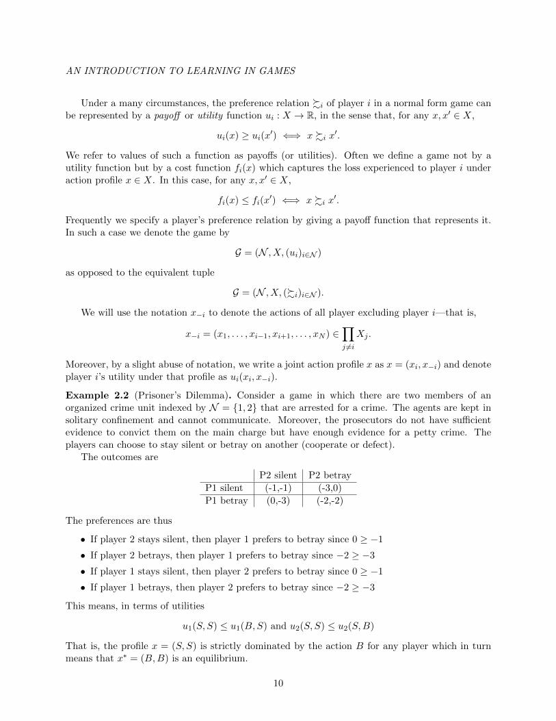
Example 2.2 (Prisoner’s Dilemma). Consider a game in which there are two members of anorganized crime unit indexed by N = 1, 2 that are arrested for a crime. The agents are kept insolitary confinement and cannot communicate. Moreover, the prosecutors do not have sufficientevidence to convict them on the main charge but have enough evidence for a petty crime. Theplayers can choose to stay silent or betray on another (cooperate or defect).
The outcomes are
P2 silent P2 betray
P1 silent (-1,-1) (-3,0)
P1 betray (0,-3) (-2,-2)
The preferences are thus
• If player 2 stays silent, then player 1 prefers to betray since 0 ≥ −1
• If player 2 betrays, then player 1 prefers to betray since −2 ≥ −3
• If player 1 stays silent, then player 2 prefers to betray since 0 ≥ −1
• If player 1 betrays, then player 2 prefers to betray since −2 ≥ −3
This means, in terms of utilities
u1(S, S) ≤ u1(B,S) and u2(S, S) ≤ u2(S,B)
That is, the profile x = (S, S) is strictly dominated by the action B for any player which in turnmeans that x∗ = (B,B) is an equilibrium.
10
AN INTRODUCTION TO LEARNING IN GAMES
2.2 Types of Games
In this section and from here forward, we will define concepts from the perspective that playershave cost function fi and hence, are cost minimizers. When it is easier or more appropriate tohave players as utility maximizers with utility functions ui, we will make this clear in the writtencontext.
There are several ways to create a taxonomy for games. We can distinguish them based on theinformation available to agents (cf. the previous discussion on extensive form versus normal formgames), the rules of the game (e.g., order of play), or the objectives of players. Even in terms ofthe objectives, there are several ways to distinguish between games: e.g., it could be based on howpayoffs are realizes or on the assumptions of the structure or class of cost functions players use.
In the first part of these lecture notes, we will primarily focus on full information games. Whenwe go to the second part on learning in games, we will discuss partial information and differentfeedback structures on the learning process.
2.2.1 Characterizing Games Based on Rules
There are many ways in which the rules of the game can lead to methods of categorizing anddistinguishing classes of games. In this set of lecture notes, we will only discuss one main waywhich is central to a lot of game theoretic formulations: the order of play.
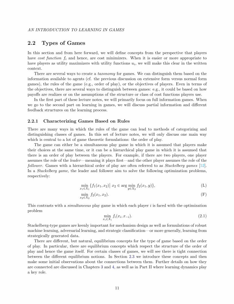
The game can either be a simultaneous play game in which it is assumed that players maketheir choices at the same time, or it can be a hierarchical play game in which it is assumed thatthere is an order of play between the players. For example, if there are two players, one playerassumes the role of the leader—meaning it plays first—and the other player assumes the role of thefollower. Games with a hierarchical order of play are often referred to as Stackelberg games [52].In a Stackelberg game, the leader and follower aim to solve the following optimization problems,respectively:
minx1∈X1
f1(x1, x2)∣∣ x2 ∈ arg min
y∈X2
f2(x1, y), (L)
minx2∈X2
f2(x1, x2). (F)
This contrasts with a simultaneous play game in which each player i is faced with the optimizationproblem
minxi∈Xi
fi(xi, x−i). (2.1)
Stackelberg-type games are keenly important for mechanism design as well as formulations of robustmachine learning, adversarial learning, and strategic classification—or more generally, learning fromstrategically generated data.
There are different, but natural, equilibrium concepts for the type of game based on the orderof play. In particular, there are equilibrium concepts which respect the structure of the order ofplay and hence the game itself. For certain classes of games, we will see there is tight connectionbetween the different equilibrium notions. In Section 2.3 we introduce these concepts and thenmake some initial observations about the connections between them. Further details on how theyare connected are discussed in Chapters 3 and 4, as well as in Part II where learning dynamics playa key role.
11
AN INTRODUCTION TO LEARNING IN GAMES
2.2.2 Characterizing Games Based on Objectives
Regarding how payoffs are realized, there are several main types of games: zero-sum games,constant-sum games, common-payoff games, and non-zero-sum games (or general-sum games).
Definition 2.3. A game G = (N , X, (fi)i∈N ) is constant sum if∑i∈N
fi(x) = c, ∀ x ∈ X, (2.2)
for some constant c. If c = 0, then the game is zero-sum, and if the game is not constant orzero-sum then it is non-zero-sum or general sum.
Prisoner’s dilemma is a type of non-zero sum game, though it gives rise to the non-intuitiveoutcome that players should choose a strategy that leads to the worst possible outcome even thoughthere is a socially cooperative solution with better payoffs across the board. Another interestingnon-zero sum game is given below.
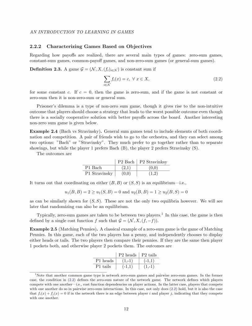
Example 2.4 (Bach vs Stravinsky). General sum games tend to include elements of both coordi-nation and competition. A pair of friends wish to go to the orchestra, and they can select amongtwo options: ”Bach” or ”Stravinsky”. They much prefer to go together rather than to separateshowings, but while the player 1 prefers Bach (B), the player 2 prefers Stravinsky (S).
The outcomes are
P2 Bach P2 Stravinksy
P1 Bach (2,1) (0,0)
P1 Stravinsky (0,0) (1,2)
It turns out that coordinating on either (B,B) or (S, S) is an equilibrium—i.e.,
u1(B,B) = 2 ≥ u1(S,B) = 0 and u2(B,B) = 1 ≥ u2(B,S) = 0
as can be similarly shown for (S, S). These are not the only two equilibria however. We will seelater that randomizing can also be an equilibrium.
Typically, zero-sum games are taken to be between two players.1 In this case, the game is thendefined by a single cost function f such that G = (N , X, (f,−f)).
Example 2.5 (Matching Pennies). A classical example of a zero-sum game is the game of MatchingPennies. In this game, each of the two players has a penny, and independently chooses to displayeither heads or tails. The two players then compare their pennies. If they are the same then player1 pockets both, and otherwise player 2 pockets them. The outcomes are
P2 heads P2 tails
P1 heads (1,-1) (-1,1)
P1 tails (-1,1) (1,-1)
1Note that another common game type is network zero-sum games and pairwise zero-sum games. In the formercase, the condition in (2.2) defines the zero-sum nature of the network game. The network defines which playerscompete with one another—i.e., cost function dependencies on player actions. In the latter case, players that competewith one another do so in pairwise zero-sum interactions. In this case, not only does (2.2) hold, but it is also the casethat fi(x) + fj(x) = 0 if in the network there is an edge between player i and player j, indicating that they competewith one another.
12
AN INTRODUCTION TO LEARNING IN GAMES
We will see that the best thing players can do (such that they do not have an incentive to deviate)is to randomize. That is, play heads and tails with equal probability.
Rock paper scissors is another common zero sum game in which there are three strategies perplayer such that rock beats scissors, paper beats rock, and scissors beat paper. In this game, it isalso an ”equilibrium” strategy to randomize.
Another important type of game is a common-payoff game or pure coordination games.
Definition 2.6. A common-payoff game is a type of constant sum game such that for all profilesx ∈ X and any two agents i and j, ui(x) = uj(x).
In such games the agents have no conflicting interests; their sole challenge is to coordinate onan action that is maximally beneficial to all.
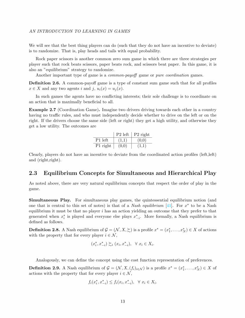
Example 2.7 (Coordination Game). Imagine two drivers driving towards each other in a countryhaving no traffic rules, and who must independently decide whether to drive on the left or on theright. If the drivers choose the same side (left or right) they get a high utility, and otherwise theyget a low utility. The outcomes are
P2 left P2 right
P1 left (1,1) (0,0)
P1 right (0,0) (1,1)
Clearly, players do not have an incentive to deviate from the coordinated action profiles (left,left)and (right,right).
2.3 Equilibrium Concepts for Simultaneous and Hierarchical Play
As noted above, there are very natural equilibrium concepts that respect the order of play in thegame.
Simultaneous Play. For simultaneous play games, the quintessential equilibrium notion (andone that is central to this set of notes) is that of a Nash equilibrium [41]. For x∗ to be a Nashequilibrium it must be that no player i has an action yielding an outcome that they prefer to thatgenerated when x∗i is played and everyone else plays x∗−i. More formally, a Nash equilibrium isdefined as follows.
Definition 2.8. A Nash equilibrium of G = (N , X,%) is a profile x∗ = (x∗1, . . . , x∗N ) ∈ X of actions
with the property that for every player i ∈ N ,
(x∗i , x∗−i) %i (xi, x
∗−i), ∀ xi ∈ Xi.
Analogously, we can define the concept using the cost function representation of preferences.
Definition 2.9. A Nash equilibrium of G = (N , X, (fi)i∈N ) is a profile x∗ = (x∗1, . . . , x∗N ) ∈ X of
actions with the property that for every player i ∈ N ,
fi(x∗i , x∗−i) ≤ fi(xi, x∗−i), ∀ xi ∈ Xi.
13
AN INTRODUCTION TO LEARNING IN GAMES
Another useful concept is the best response set with which we can restate the above definition.For any x−i ∈ X−i define Bi(x−i) to be
Bi(x−i) = xi| fi(xi, x−i) ≤ fi(x′i, x−i), ∀ x′i ∈ Xi.
Definition 2.10. A Nash equilibrium is an action profile x∗ = (x∗1, . . . , x∗N ) ∈ X for which
x∗i ∈ Bi(x∗−i), ∀ i.
An alternative expression which gives us some intuition for refinements of Nash is to write thebest response map as follows:
x∗i ∈ arg minxi
fi(xi, x∗−i)
The action spaces Xi can be finite or infinite—in particular, a continuum.2 In either case,both definitions above for Nash can be seen as defining a pure strategy Nash equilibrium or a Nashequilibrium in pure strategies. Furthermore, if the action spaces are finite—say Xi = 1, . . . ,mibut we consider the probability simplex
∆(Xi) =
xi :
mi∑j=1
xij = 1, 0 ≤ xij ≤ 1
then the definitions above capture mixed strategy Nash equilibria where each x∗ij denotes the prob-ability that player i will player strategy j ∈ Xi in equilibrium. This distinction between pure andmixed strategy equilibrium concepts will be further discussed in the subsequent chapters.
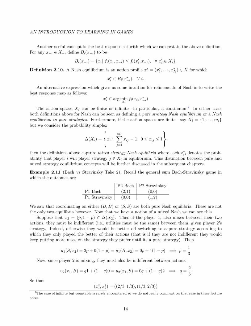
Example 2.11 (Bach vs Stravinsky Take 2). Recall the general sum Bach-Stravinsky game inwhich the outcomes are
P2 Bach P2 Stravinksy
P1 Bach (2,1) (0,0)
P1 Stravinsky (0,0) (1,2)
We saw that coordinating on either (B,B) or (S, S) are both pure Nash equilibria. These are notthe only two equilibria however. Now that we have a notion of a mixed Nash we can see this.
Suppose that x2 = (p, 1 − p) ∈ ∆(X2). Then if the player 1, also mixes between their twoactions, they must be indifferent (i.e., utilities must be the same) between them, given player 2’sstrategy. Indeed, otherwise they would be better off switching to a pure strategy according towhich they only played the better of their actions (that is if they are not indifferent they wouldkeep putting more mass on the strategy they prefer until its a pure strategy). Then
u1(S, x2) = 2p+ 0(1− p) = u1(B, x2) = 0p+ 1(1− p) =⇒ p =1
3
Now, since player 2 is mixing, they must also be indifferent between actions:
u2(x1, B) = q1 + (1− q)0 = u2(x1, S) = 0q + (1− q)2 =⇒ q =2
3
So that(x∗1, x
∗2) = ((2/3, 1/3), (1/3, 2/3))
2The case of infinite but countable is rarely encountered so we do not really comment on that case in these lecturenotes.
14
AN INTRODUCTION TO LEARNING IN GAMES
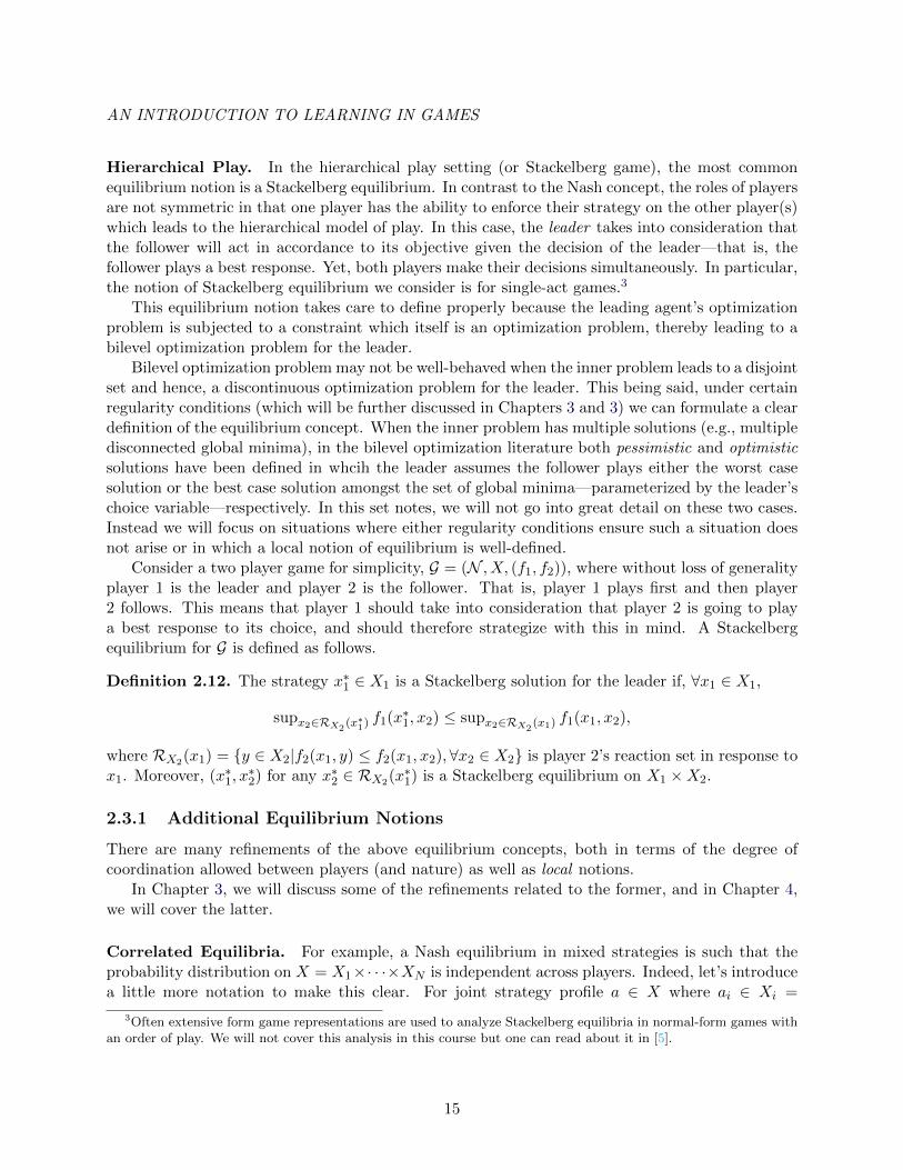
Hierarchical Play. In the hierarchical play setting (or Stackelberg game), the most commonequilibrium notion is a Stackelberg equilibrium. In contrast to the Nash concept, the roles of playersare not symmetric in that one player has the ability to enforce their strategy on the other player(s)which leads to the hierarchical model of play. In this case, the leader takes into consideration thatthe follower will act in accordance to its objective given the decision of the leader—that is, thefollower plays a best response. Yet, both players make their decisions simultaneously. In particular,the notion of Stackelberg equilibrium we consider is for single-act games.3
This equilibrium notion takes care to define properly because the leading agent’s optimizationproblem is subjected to a constraint which itself is an optimization problem, thereby leading to abilevel optimization problem for the leader.
Bilevel optimization problem may not be well-behaved when the inner problem leads to a disjointset and hence, a discontinuous optimization problem for the leader. This being said, under certainregularity conditions (which will be further discussed in Chapters 3 and 3) we can formulate a cleardefinition of the equilibrium concept. When the inner problem has multiple solutions (e.g., multipledisconnected global minima), in the bilevel optimization literature both pessimistic and optimisticsolutions have been defined in whcih the leader assumes the follower plays either the worst casesolution or the best case solution amongst the set of global minima—parameterized by the leader’schoice variable—respectively. In this set notes, we will not go into great detail on these two cases.Instead we will focus on situations where either regularity conditions ensure such a situation doesnot arise or in which a local notion of equilibrium is well-defined.
Consider a two player game for simplicity, G = (N , X, (f1, f2)), where without loss of generalityplayer 1 is the leader and player 2 is the follower. That is, player 1 plays first and then player2 follows. This means that player 1 should take into consideration that player 2 is going to playa best response to its choice, and should therefore strategize with this in mind. A Stackelbergequilibrium for G is defined as follows.
Definition 2.12. The strategy x∗1 ∈ X1 is a Stackelberg solution for the leader if, ∀x1 ∈ X1,
supx2∈RX2(x∗1) f1(x∗1, x2) ≤ supx2∈RX2
(x1) f1(x1, x2),
where RX2(x1) = y ∈ X2|f2(x1, y) ≤ f2(x1, x2), ∀x2 ∈ X2 is player 2’s reaction set in response tox1. Moreover, (x∗1, x
∗2) for any x∗2 ∈ RX2(x∗1) is a Stackelberg equilibrium on X1 ×X2.
2.3.1 Additional Equilibrium Notions
There are many refinements of the above equilibrium concepts, both in terms of the degree ofcoordination allowed between players (and nature) as well as local notions.
In Chapter 3, we will discuss some of the refinements related to the former, and in Chapter 4,we will cover the latter.
Correlated Equilibria. For example, a Nash equilibrium in mixed strategies is such that theprobability distribution on X = X1×· · ·×XN is independent across players. Indeed, let’s introducea little more notation to make this clear. For joint strategy profile a ∈ X where ai ∈ Xi =
3Often extensive form game representations are used to analyze Stackelberg equilibria in normal-form games withan order of play. We will not cover this analysis in this course but one can read about it in [5].
15
AN INTRODUCTION TO LEARNING IN GAMES
1, . . . ,mi and a−i ∈ X−i, we denote the expected utility given the mixed strategy x =∏i∈N xi
byEa∼x[ui(ai, a−i)]
Here strategies ai are sampled from xi independently across players as the notation x =∏i∈N xi
indicates. If on the other hand, players are allowed to coordinate via an external signal or recom-mendation, then the distribution x is no longer independent across players, and this leads to thenotion of a correlated equilbirium. This is the first natural refinement of a Nash equilibrium. Thatis, all Nash equilibria are correlated equilibria but the other direction does not hold:
Pure Nash ⊂ Mixed Nash ⊂ Correlated Equilibria
This is an important refinement since many learning algorithms for mixed strategies in finite gamescan only be guaranteed to achieve correlated equilibria.
Recall that in a Nash equilibrium, players randomize over strategies independently. This is oneof the primary distinctions between mixed Nash equilibria and correlated equilibria: in a correlatedequilibrium there is a correlating mechanism (signal) that the agents use as a reference point indetermining a utility maximizing strategy. Due to this, the agents are no longer randomizingindependently.
In fact, it may be the case for games with multiple Nash equilibria that we want to allow forrandomization between Nash equilibria by some form of communication prior to the play of thegame. Consider the following example in which the coordinating mechanism is a coin flip (Bernoullirandom variable).
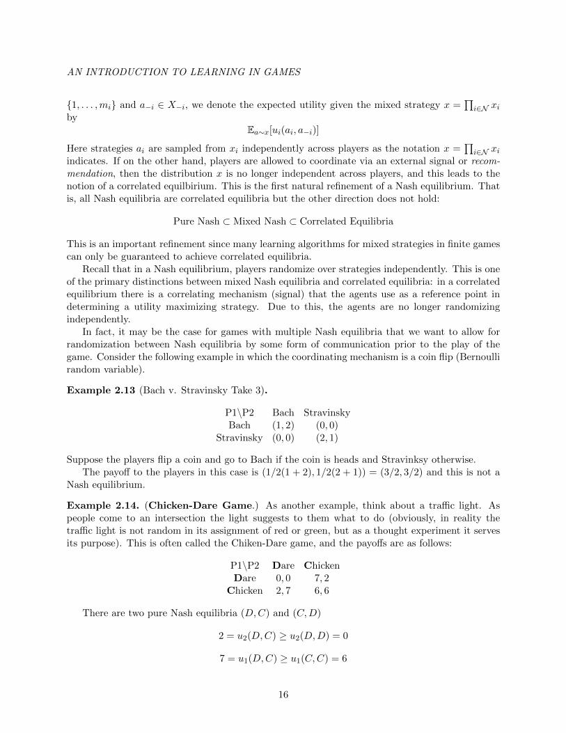
Example 2.13 (Bach v. Stravinsky Take 3).
P1\P2 Bach StravinskyBach (1, 2) (0, 0)
Stravinsky (0, 0) (2, 1)
Suppose the players flip a coin and go to Bach if the coin is heads and Stravinksy otherwise.The payoff to the players in this case is (1/2(1 + 2), 1/2(2 + 1)) = (3/2, 3/2) and this is not a
Nash equilibrium.
Example 2.14. (Chicken-Dare Game.) As another example, think about a traffic light. Aspeople come to an intersection the light suggests to them what to do (obviously, in reality thetraffic light is not random in its assignment of red or green, but as a thought experiment it servesits purpose). This is often called the Chiken-Dare game, and the payoffs are as follows:
P1\P2 Dare ChickenDare 0, 0 7, 2
Chicken 2, 7 6, 6
There are two pure Nash equilibria (D,C) and (C,D)
2 = u2(D,C) ≥ u2(D,D) = 0
7 = u1(D,C) ≥ u1(C,C) = 6
16

AN INTRODUCTION TO LEARNING IN GAMES
and one mixed Nash where the probability of ((D,C), (D,C)) is ((1/3, 2/3), (1/3, 2/3)):[1323
]> [0 72 6
] [1323
]=
[43193
]> [1212
]= 4.667 =
14
3≥[ab
]> [0 72 6
] [1212
]=
[ab
]> [143143
]=
14
3(a+ b) =
14
3
Now suppose that prior to playing the game the players performed the following experiment:
• Player 1 chooses ball from bag with three balls labeled C,C,D
• Player 2 chooses ball from bag with remaining two balls
• Player 1 and player 2 play according to the ball they get
It can be verified that there is no incentive to deviate from such an agreement since the suggestedstrategy is best in expectation.
This experiment is equivalent to having the following strategy profile chosen for the players bysome third party, a correlation device:
Dare ChickenDare 0 1/3
Chicken 1/3 1/3
Suppose player 1 gets a ball with C. Then player 2 will play C with probability 1/2 and d withprobability 1/2. The expected utility of D is 0(1/2) + 7(1/2) = 3.5 and the expected utility of Cout is 2(1/2)+6(1/2) = 4. So, the player would prefer to Chicken out. On the other hand, supposeplayer 1 gets ball D, he would not want to deviate supposing the other player played their assignedstrategy since he will get 7 (the highest payoff possible).
The expected payoff for this game is 7(1/3) + 2(1/3) + 6(1/3) = 5 which is greater than theNash payoff 14/3.
This equilibrium (using the correlation device) is a correlated equilibrium since the players playis correlated.
Local notions of Equilibria. The other type of refinement is more natural for pure strategyequilibria in games on continuous actions spaces. In many settings—particularly those relevantfor machine learning and learning-based systems—the cost functions of players are non-convex andhence, we consider local notions of equilibria. That is, equilibria such as Nash or Stackelberg definedin a local neighborhood. This will be covered in more detail in Chapter 4. As with correlatedequilibria, the local notions of equilibria are important because again many learning algorithmsonly have local guarantees on convergence due to the non-convex optimization landscape in whichplayers are interacting.
For instance, we can define a δ-local Nash equilibrium as follows. Let Bδ(xi) be the δ–radiusball centered at x in the Euclidean space Rmi endowed with the usual metric.
Definition 2.15. A joint action profile x∗ is an local Nash equilibrium if there exists a δ > 0 suchthat
fi(x∗i , x∗−i) ≤ fi(xi, x∗−i), ∀xi ∈ Bδ(x∗i )
17
AN INTRODUCTION TO LEARNING IN GAMES
Approximate notions of Equilibria. Yet, another refinement arises due to approximation ofthe inequalities in the definition of equilibrium concepts such as Nash or Stackelberg. For instance,we can define an ε-approximate Nash equilibrium as follows. Let Bδ(xi) be the δ–radius ballcentered at x in the Euclidean space Rmi endowed with the usual metric.
Definition 2.16. Give ε, δ > 0, a joint action profile x∗ is an (ε, δ)-approximate Nash equilibriumif
fi(x∗i , x∗−i) ≤ fi(xi, x∗−i) + ε, ∀xi ∈ Bδ(x∗i )
18
Chapter 3
Games on Finite Action Spaces
3.1 Introduction
Normal form games in which the action spaces Xi for each player i ∈ N is itself a finite set arecalled finite games or normal form games on finite action spaces. In this case, we can define orrepresent the action space for a player i as an index set as follows:
Xi = 1, . . . ,mi
where mi = |Xi| is the number of actions available to player i.The utility of player i is still a mapping from the joint action space X to a real number.
For this class of games there are two relevant types of equilibrium concepts: pure strategy/actionequilibria and mixed strategy/action equilibria. Both are defined as in the previous chapter for aNash equilibrium. That is,
ui(x∗i , x∗−i) ≥ ui(xi, x∗−i), ∀xi ∈ Xi
where if we are considering pure strategy Nash equilibria then xi ∈ Xi = 1, . . . ,mi and if we areconsidering mixed Nash equilibria, then xi ∈ ∆(Xi)—i.e., the probability simplex on 1, . . . ,miwhich is defined by
∆(Xi) =
xi :
mi∑j=1
xij = 1, 0 ≤ xij ≤ 1
The use of xi for both pure and mixed strategies is of course an abuse of notation in some sense,however, for xi ∈ ∆(Xi), the strategy
xi = (0, . . . , 0, 1︸︷︷︸j-th entry
, 0, . . . , 0)
represents a pure strategy where player i puts all the mass on the j-th entry. Since this is an abuseof notation of sorts, using xi for both pure and mixed strategies, so we will be very clear what weare referring depending on the context moving forward. When we are discussing mixed strategies,we will use xi for the mixed strategy and either an index such as j ∈ Xi or si ∈ Xi for the purestrategy. In the case of mixed Nash equilibria, we can write the utility as
ui(xi, x−i) =
mi∑j=1
xijui(j, x−i)
19
AN INTRODUCTION TO LEARNING IN GAMES
where ui(j, x−i) is the utility player i gets from playing the pure strategy j given that the remainingplayers are playing the mixed strategy x−i.
One reasonable interpretation for mixed policies is the following. Suppose players are playing agame repeatedly. In each game they choose their actions randomly according to pre-selected mixedpolicies (independently from each other and independently from game to game) and their goal isto minimize/maximize the cost/reward averaged over all the games played.
Moreover, by introducing mixed policies, we essentially enlarged the action spaces for bothplayers and a consequence of this enlargement is that saddle-point equilibria now always exist.Indeed, this is exactly Nash’s celebrated theorem provides existence in the class of finite games.
Theorem 3.1 (Nash ’51). Every game with a finite number of players and action profiles has atleast one Nash equilibrium.
The proof of this result takes time to go through, and we do not discuss it here except tomention that it is typically achieved by appealing to a fixed-point theorem from mathematics, suchas those due to Kakutani and Brouwer. Nash’s theorem depends critically on the availability ofmixed strategies to the agents. However, this does not mean that an agent plays a mixed-strategyNash equilibrium: Do players really sample probability distributions in their heads? Some peoplehave argued that they really do, and there is some empirical backing of this.
3.2 Matrix Games: General Sum
A finite normal form game in which there are two players can be described conveniently in a tableor matrix form. When there are multiple players (here meaning more than two), the finite normalform game can be represented as a tensor. If it is further the case that there are more than twoplayers and the game is such that it can be written as pairwise games between players, then werefer to such games as polymatrix games or network matrix games.
For simplicity we will focus on two-player bi-matrix games. Each player has a a finite set ofactions:
• player 1 has m actions, indexed by X1 = 1, . . . ,m• player 2 has n actions, indexed by X2 = 1, . . . , n
The outcome of the game for player 1 is quantified by an m × n matrix A = [aij ], and similarly,for player 2, the outcome is quantified by an n×m matrix B = [bji]. In particular, the entry aij ofthe matrix provides the outcome of the game when player 1 selects an action i ∈ 1, . . . ,m, andplayer 2 selects an action j ∈ 1, . . . , n. The utilities1 of the players are then written as
u1(x1, x2) = x>1 Ax2 and u2(x1, x2) = x>1 B>x2.
One can imagine that player 1 selects a row of A and player 2 selects a column of B>.The tuple G = (A,B) denotes the bimatrix game in which player 1 has utility u1(x1, x2) =
x>1 Ax2 and player 2 has utility u2(x1, x2) = x>1 B>x2.
1Note that different references treat the payoff of the ”column” player (i.e. player 2) differently in that they maydefine B using the transpose of the above. So take care when reading other references to understand their notion.
20
AN INTRODUCTION TO LEARNING IN GAMES
Definition 3.2. A joint action profile (x∗1, x∗2) ∈ ∆(X1) × ∆(X2) is a Nash equilibrium for the
game G = (A,B) if(x∗1)>Ax∗2 ≥ x>1 Ax∗2, ∀ x1 ∈ ∆(X1)
and(x∗1)>B>x∗2 ≥ (x∗1)>B>x2, ∀ x2 ∈ ∆(X2)
Note that if the matrices A and B represent costs to players, then the inequalities in the abovedefinition simply flip.
Example 3.3 (General Sum Bi-matrix Game). Consider the following general sum game:
P1\P2 L RU (5, 1) (0, 0)D (4, 4) (1, 5)
The matrix form of this game is defined by the following matrices:
A =
[5 04 1
]and B> =
[1 04 5
]One can easily see that (U,L) and (D,R) are the two pure strategy NE of the game.
For a purely mixed strategy, recall that if one player mixes, then the other player should beindifferent between the outcomes of its actions since otherwise it would put all the mass on thepreferred action. We can express this in terms of the matrices. Let a>i be the i-th row of A and bjbe the j-th column of B>. Then, if player 1 uses the mixed strategy x1 = (p, 1 − p), it should bethe case for player 2 that it is indifferent between actions L and R. That is,
x>1 b1 = x>1 b2 ⇐⇒ p+ 4(1− p) = 0p+ 5(1− p) ⇐⇒ p = 12
Similarly, if player 2 uses the mixed strategy x2 = (q, 1− q), it should be the case that player 1 isindifferent between U and D. That is,
a>1 x2 = a>2 x2 ⇐⇒ 5q + 0(1− q) = 4q + (1− q) ⇐⇒ q = 12
Thus, the unique Nash is (12 ,
12 ,
12 ,
12) and the payoff to players is (5/2, 5/2).
This example provides some intuition for how we will ultimately pose finding Nash in bimatrixgames as an optimization problem.
3.3 Bi-Matrix Games: Zero Sum
It is even simpler in the zero-sum setting since only a single matrix is needed to define the game.In particular, player 1 wants to minimize the outcome A(i, j) and player 2 wants to maximizeA(i, j). For simplicity, since there are two players, in this section we will use x ∈ X = ∆(X) withX = 1, . . . ,m for player 1’s mixed strategy and y ∈ Y = ∆(Y ) with Y = 1, . . . , n for player2’s mixed strategy. Then A ∈ Rm×n and the game is defined by payoff matrices A and B = −A>where player 1 has cost
f(x, y) = x>Ay
and player 2 has cost−f(x, y) = −x>Ay
21
AN INTRODUCTION TO LEARNING IN GAMES
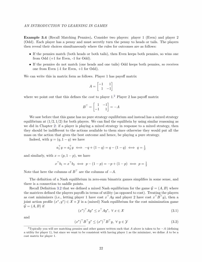
Example 3.4 (Recall Matching Pennies). Consider two players: player 1 (Even) and player 2(Odd). Each player has a penny and must secretly turn the penny to heads or tails. The playersthen reveal their choices simultaneously where the rules for outcomes are as follows:
• If the pennies match (both heads or both tails), then Even keeps both pennies, so wins onefrom Odd (+1 for Even, -1 for Odd).
• If the pennies do not match (one heads and one tails) Odd keeps both pennies, so receivesone from Even (-1 for Even, +1 for Odd).
We can write this in matrix form as follows. Player 1 has payoff matrix
A =
[−1 1
1 −1
]where we point out that this defines the cost to player 1.2 Player 2 has payoff matrix
B> =
[1 −1−1 1
]= −A
We saw before that this game has no pure strategy equilibrium and instead has a mixed strategyequilibrium at (1/2, 1/2) for both players. We can find the equilibria by using similar reasoning aswe did in Chapter 2: if a player is playing a mixed strategy in response to a mixed strategy, thenthey should be indifferent to the actions available to them since otherwise they would put all themass on the action that gives the best outcome and hence, be playing a pure strategy.
Indeed, with y = (q, 1− q) we have
a>1 y = a>2 y ⇐⇒ −q + (1− q) = q − (1− q) ⇐⇒ q = 12
and similarly, with x = (p, 1− p), we have
x>b1 = x>b2 ⇐⇒ p− (1− p) = −p+ (1− p) ⇐⇒ p = 12
Note that here the columns of B> are the columns of −A.
The definition of a Nash equilibrium in zero-sum bimatrix games simplifies in some sense, andthere is a connection to saddle points.
Recall Definition 3.2 that we defined a mixed Nash equilibrium for the game G = (A,B) wherethe matrices defined the players payoffs in terms of utility (as opposed to cost). Treating the playersas cost minimizers (i.e., letting player 1 have cost x>Ay and player 2 have cost x>B>y), then ajoint action profile (x∗, y∗) ∈ X ×Y is a (mixed) Nash equilibrium for the cost minimization gameG = (A,B) if
(x∗)>Ay∗ ≤ x>Ay∗, ∀ x ∈ X (3.1)
and(x∗)>B>y∗ ≤ (x∗)>B>y, ∀ y ∈ Y (3.2)
2Typically you will see matching pennies and other games written such that A above is taken to be −A (defininga utility for player 1), but since we want to be consistent with having player 1 as the minimizer, we define A to be acost matrix for player 1.
22
AN INTRODUCTION TO LEARNING IN GAMES
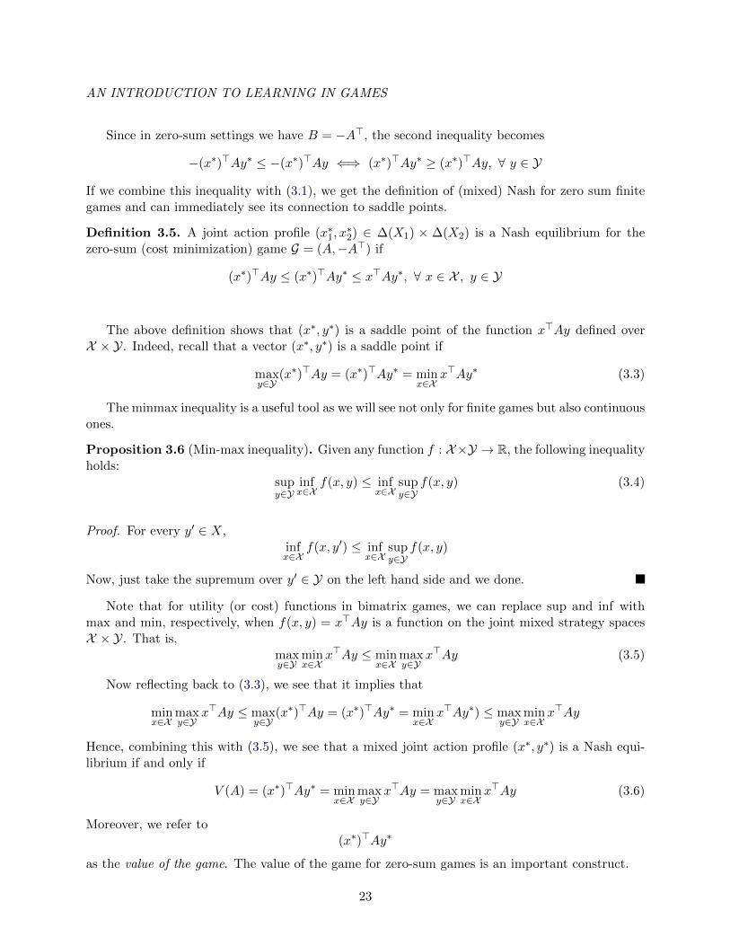
Since in zero-sum settings we have B = −A>, the second inequality becomes
−(x∗)>Ay∗ ≤ −(x∗)>Ay ⇐⇒ (x∗)>Ay∗ ≥ (x∗)>Ay, ∀ y ∈ Y
If we combine this inequality with (3.1), we get the definition of (mixed) Nash for zero sum finitegames and can immediately see its connection to saddle points.
Definition 3.5. A joint action profile (x∗1, x∗2) ∈ ∆(X1) × ∆(X2) is a Nash equilibrium for the
zero-sum (cost minimization) game G = (A,−A>) if
(x∗)>Ay ≤ (x∗)>Ay∗ ≤ x>Ay∗, ∀ x ∈ X , y ∈ Y
The above definition shows that (x∗, y∗) is a saddle point of the function x>Ay defined overX × Y. Indeed, recall that a vector (x∗, y∗) is a saddle point if
maxy∈Y
(x∗)>Ay = (x∗)>Ay∗ = minx∈X
x>Ay∗ (3.3)
The minmax inequality is a useful tool as we will see not only for finite games but also continuousones.
Proposition 3.6 (Min-max inequality). Given any function f : X×Y → R, the following inequalityholds:
supy∈Y
infx∈X
f(x, y) ≤ infx∈X
supy∈Y
f(x, y) (3.4)
Proof. For every y′ ∈ X,infx∈X
f(x, y′) ≤ infx∈X
supy∈Y
f(x, y)
Now, just take the supremum over y′ ∈ Y on the left hand side and we done.
Note that for utility (or cost) functions in bimatrix games, we can replace sup and inf withmax and min, respectively, when f(x, y) = x>Ay is a function on the joint mixed strategy spacesX × Y. That is,
maxy∈Y
minx∈X
x>Ay ≤ minx∈X
maxy∈Y
x>Ay (3.5)
Now reflecting back to (3.3), we see that it implies that
minx∈X
maxy∈Y
x>Ay ≤ maxy∈Y
(x∗)>Ay = (x∗)>Ay∗ = minx∈X
x>Ay∗) ≤ maxy∈Y
minx∈X
x>Ay
Hence, combining this with (3.5), we see that a mixed joint action profile (x∗, y∗) is a Nash equi-librium if and only if
V (A) = (x∗)>Ay∗ = minx∈X
maxy∈Y
x>Ay = maxy∈Y
minx∈X
x>Ay (3.6)
Moreover, we refer to(x∗)>Ay∗
as the value of the game. The value of the game for zero-sum games is an important construct.
23
AN INTRODUCTION TO LEARNING IN GAMES
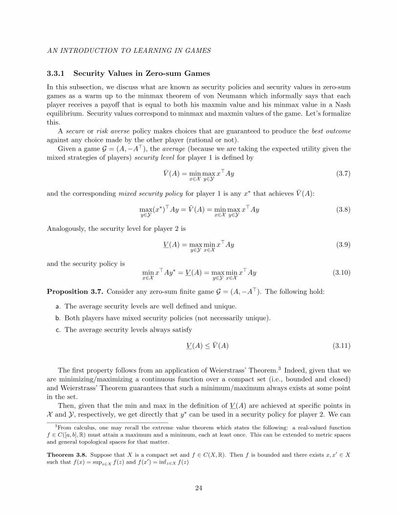
3.3.1 Security Values in Zero-sum Games
In this subsection, we discuss what are known as security policies and security values in zero-sumgames as a warm up to the minmax theorem of von Neumann which informally says that eachplayer receives a payoff that is equal to both his maxmin value and his minmax value in a Nashequilibrium. Security values correspond to minmax and maxmin values of the game. Let’s formalizethis.
A secure or risk averse policy makes choices that are guaranteed to produce the best outcomeagainst any choice made by the other player (rational or not).
Given a game G = (A,−A>), the average (because we are taking the expected utility given themixed strategies of players) security level for player 1 is defined by
V (A) = minx∈X
maxy∈Y
x>Ay (3.7)
and the corresponding mixed security policy for player 1 is any x∗ that achieves V (A):
maxy∈Y
(x∗)>Ay = V (A) = minx∈X
maxy∈Y
x>Ay (3.8)
Analogously, the security level for player 2 is
V (A) = maxy∈Y
minx∈X
x>Ay (3.9)
and the security policy isminx∈X
x>Ay∗ = V (A) = maxy∈Y
minx∈X
x>Ay (3.10)
Proposition 3.7. Consider any zero-sum finite game G = (A,−A>). The following hold:
a. The average security levels are well defined and unique.
b. Both players have mixed security policies (not necessarily unique).
c. The average security levels always satisfy
V (A) ≤ V (A) (3.11)
The first property follows from an application of Weierstrass’ Theorem.3 Indeed, given that weare minimizing/maximizing a continuous function over a compact set (i.e., bounded and closed)and Weierstrass’ Theorem guarantees that such a minimum/maximum always exists at some pointin the set.
Then, given that the min and max in the definition of V (A) are achieved at specific points inX and Y, respectively, we get directly that y∗ can be used in a security policy for player 2. We can
3From calculus, one may recall the extreme value theorem which states the following: a real-valued functionf ∈ C([a, b],R) must attain a maximum and a minimum, each at least once. This can be extended to metric spacesand general topological spaces for that matter.
Theorem 3.8. Suppose that X is a compact set and f ∈ C(X,R). Then f is bounded and there exists x, x′ ∈ Xsuch that f(x) = supz∈X f(z) and f(x′) = infz∈X f(z)
24
AN INTRODUCTION TO LEARNING IN GAMES
reason in a similar way for player 1. Hence, this shows that the second point in Proposition 3.7holds.
The inequality in the last property follows from the minmax inequality discussed above. More-over, it is not hard to show that
V (A) ≤ mini∈X
maxj∈Y
A(i, j)
andmaxj∈Y
mini∈X
A(i, j) ≤ V (A)
That is, the mixed security levels are bounded by the pure security levels—i.e., equivalent securitylevel concept considering only pure strategies (i, j) ∈ X × Y .
Now, reflecting back to (3.6), we can state the existence of a mixed Nash equilibrium in termsof the security levels of the game.
Theorem 3.9. Given a zero-sum finite matrix game G = (A,−A>), a mixed Nash equilibriumexists if and only if
maxy∈Y
minx∈X
x>Ay = V (A) = minx∈X
maxy∈Y
x>Ay = V (A)
This is actually known as the Minmax Theorem. We will see its proof in the next section.Before getting into the next example, we need the following lemma about optimizing linear
functions over the simplex.
Proposition 3.10. Consider the simplex ∆(X) = x ∈ Rm :∑
i xi = 1, xi ≥ 0, ∀i. Suppose weaim to optimize f(x) =
∑mi=1 aixi. Then,
minx∈∆(X)
f(x) = mini∈1,...,m
ai, maxx∈∆(X)
f(x) = maxi∈1,...,m
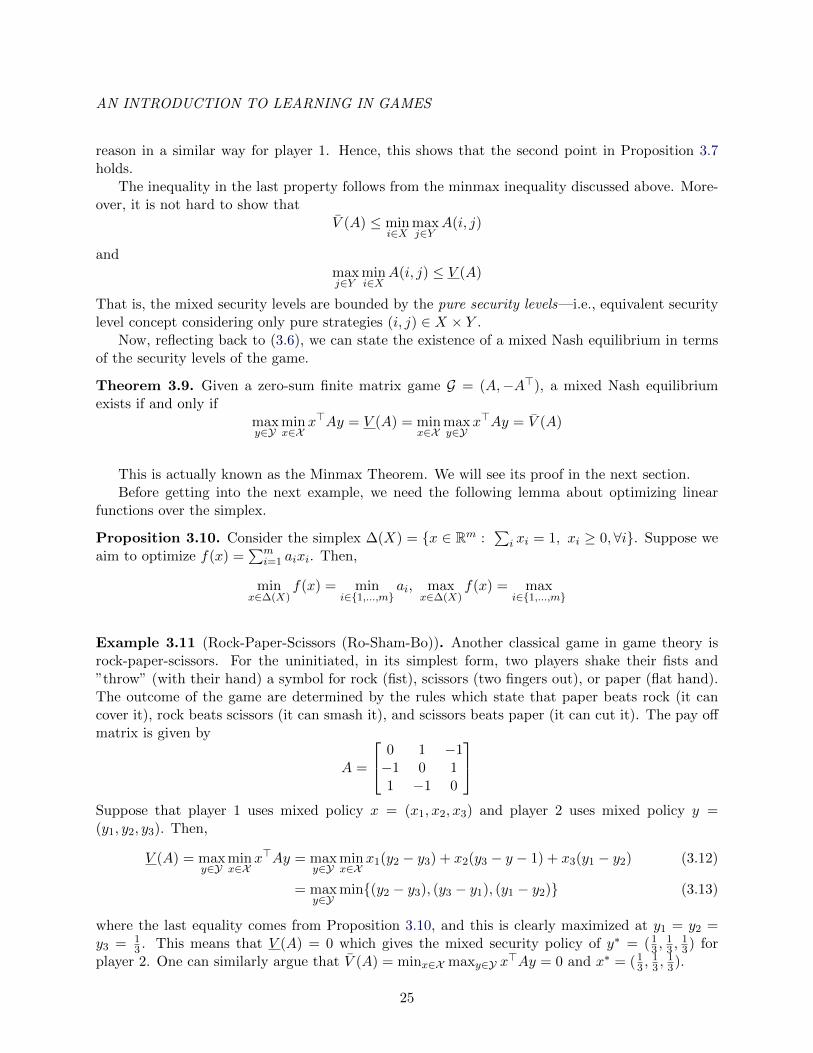
Example 3.11 (Rock-Paper-Scissors (Ro-Sham-Bo)). Another classical game in game theory isrock-paper-scissors. For the uninitiated, in its simplest form, two players shake their fists and”throw” (with their hand) a symbol for rock (fist), scissors (two fingers out), or paper (flat hand).The outcome of the game are determined by the rules which state that paper beats rock (it cancover it), rock beats scissors (it can smash it), and scissors beats paper (it can cut it). The pay offmatrix is given by
A =
0 1 −1−1 0 11 −1 0
Suppose that player 1 uses mixed policy x = (x1, x2, x3) and player 2 uses mixed policy y =(y1, y2, y3). Then,
V (A) = maxy∈Y
minx∈X
x>Ay = maxy∈Y
minx∈X
x1(y2 − y3) + x2(y3 − y − 1) + x3(y1 − y2) (3.12)
= maxy∈Y
min(y2 − y3), (y3 − y1), (y1 − y2) (3.13)
where the last equality comes from Proposition 3.10, and this is clearly maximized at y1 = y2 =y3 = 1
3 . This means that V (A) = 0 which gives the mixed security policy of y∗ = (13 ,
13 ,
13) for
player 2. One can similarly argue that V (A) = minx∈X maxy∈Y x>Ay = 0 and x∗ = (1
3 ,13 ,
13).
25
AN INTRODUCTION TO LEARNING IN GAMES
Perhaps unsurprisingly, V (A) = V (A) = V (A) = 0 and thus we have a mixed strategy equilir-bium:
(x∗, y∗) = ((13 ,
13 ,
13), (1
3 ,13 ,
13))
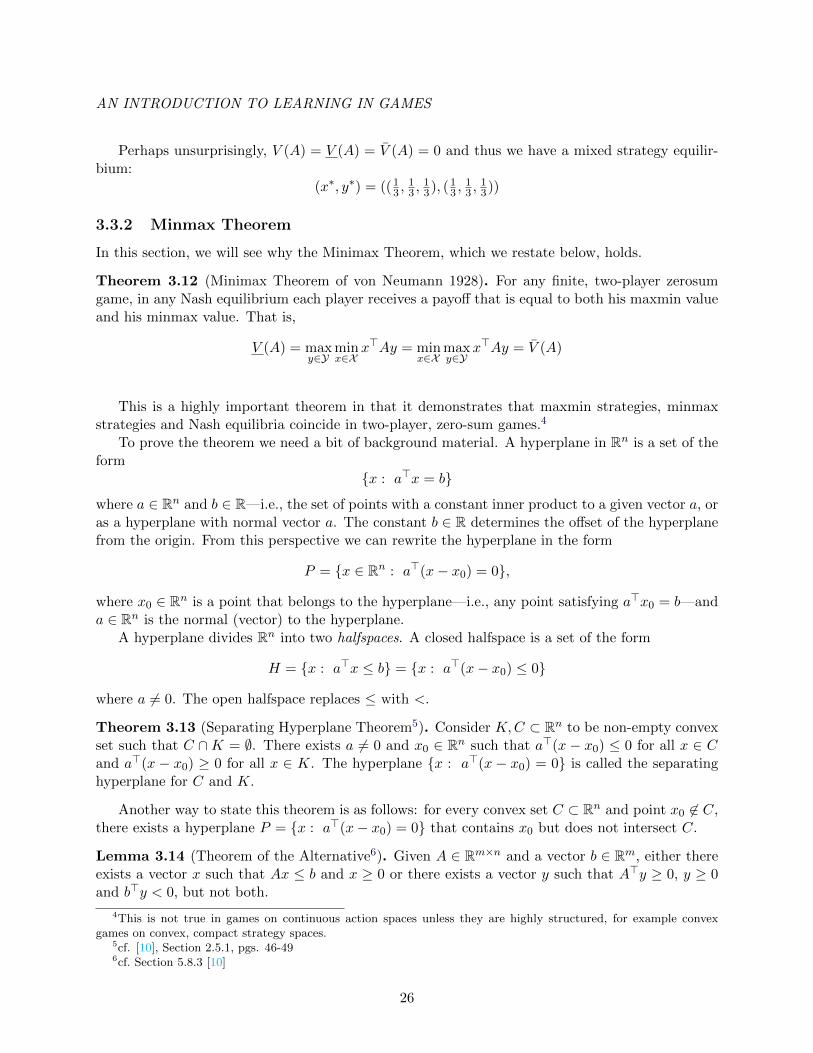
3.3.2 Minmax Theorem
In this section, we will see why the Minimax Theorem, which we restate below, holds.
Theorem 3.12 (Minimax Theorem of von Neumann 1928). For any finite, two-player zerosumgame, in any Nash equilibrium each player receives a payoff that is equal to both his maxmin valueand his minmax value. That is,
V (A) = maxy∈Y
minx∈X
x>Ay = minx∈X
maxy∈Y
x>Ay = V (A)
This is a highly important theorem in that it demonstrates that maxmin strategies, minmaxstrategies and Nash equilibria coincide in two-player, zero-sum games.4
To prove the theorem we need a bit of background material. A hyperplane in Rn is a set of theform
x : a>x = b
where a ∈ Rn and b ∈ R—i.e., the set of points with a constant inner product to a given vector a, oras a hyperplane with normal vector a. The constant b ∈ R determines the offset of the hyperplanefrom the origin. From this perspective we can rewrite the hyperplane in the form
P = x ∈ Rn : a>(x− x0) = 0,
where x0 ∈ Rn is a point that belongs to the hyperplane—i.e., any point satisfying a>x0 = b—anda ∈ Rn is the normal (vector) to the hyperplane.
A hyperplane divides Rn into two halfspaces. A closed halfspace is a set of the form
H = x : a>x ≤ b = x : a>(x− x0) ≤ 0
where a 6= 0. The open halfspace replaces ≤ with <.
Theorem 3.13 (Separating Hyperplane Theorem5). Consider K,C ⊂ Rn to be non-empty convexset such that C ∩K = ∅. There exists a 6= 0 and x0 ∈ Rn such that a>(x − x0) ≤ 0 for all x ∈ Cand a>(x − x0) ≥ 0 for all x ∈ K. The hyperplane x : a>(x − x0) = 0 is called the separatinghyperplane for C and K.
Another way to state this theorem is as follows: for every convex set C ⊂ Rn and point x0 6∈ C,there exists a hyperplane P = x : a>(x− x0) = 0 that contains x0 but does not intersect C.
Lemma 3.14 (Theorem of the Alternative6). Given A ∈ Rm×n and a vector b ∈ Rm, either thereexists a vector x such that Ax ≤ b and x ≥ 0 or there exists a vector y such that A>y ≥ 0, y ≥ 0and b>y < 0, but not both.
4This is not true in games on continuous action spaces unless they are highly structured, for example convexgames on convex, compact strategy spaces.
5cf. [10], Section 2.5.1, pgs. 46-496cf. Section 5.8.3 [10]
26
AN INTRODUCTION TO LEARNING IN GAMES
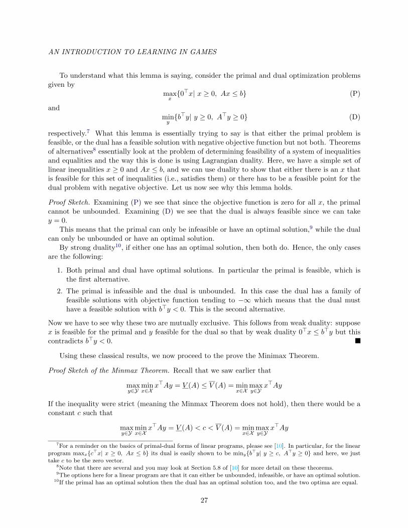
To understand what this lemma is saying, consider the primal and dual optimization problemsgiven by
maxx0>x| x ≥ 0, Ax ≤ b (P)
andminyb>y| y ≥ 0, A>y ≥ 0 (D)
respectively.7 What this lemma is essentially trying to say is that either the primal problem isfeasible, or the dual has a feasible solution with negative objective function but not both. Theoremsof alternatives8 essentially look at the problem of determining feasibility of a system of inequalitiesand equalities and the way this is done is using Lagrangian duality. Here, we have a simple set oflinear inequalities x ≥ 0 and Ax ≤ b, and we can use duality to show that either there is an x thatis feasible for this set of inequalities (i.e., satisfies them) or there has to be a feasible point for thedual problem with negative objective. Let us now see why this lemma holds.
Proof Sketch. Examining (P) we see that since the objective function is zero for all x, the primalcannot be unbounded. Examining (D) we see that the dual is always feasible since we can takey = 0.
This means that the primal can only be infeasible or have an optimal solution,9 while the dualcan only be unbounded or have an optimal solution.
By strong duality10, if either one has an optimal solution, then both do. Hence, the only casesare the following:
1. Both primal and dual have optimal solutions. In particular the primal is feasible, which isthe first alternative.
2. The primal is infeasible and the dual is unbounded. In this case the dual has a family offeasible solutions with objective function tending to −∞ which means that the dual musthave a feasible solution with b>y < 0. This is the second alternative.
Now we have to see why these two are mutually exclusive. This follows from weak duality: supposex is feasible for the primal and y feasible for the dual so that by weak duality 0>x ≤ b>y but thiscontradicts b>y < 0.
Using these classical results, we now proceed to the prove the Minimax Theorem.
Proof Sketch of the Minmax Theorem. Recall that we saw earlier that
maxy∈Y
minx∈X
x>Ay = V (A) ≤ V (A) = minx∈X
maxy∈Y
x>Ay
If the inequality were strict (meaning the Minmax Theorem does not hold), then there would be aconstant c such that
maxy∈Y
minx∈X
x>Ay = V (A) < c < V (A) = minx∈X
maxy∈Y
x>Ay
7For a reminder on the basics of primal-dual forms of linear programs, please see [10]. In particular, for the linearprogram maxxc>x| x ≥ 0, Ax ≤ b its dual is easily shown to be minyb>y| y ≥ c, A>y ≥ 0 and here, we justtake c to be the zero vector.
8Note that there are several and you may look at Section 5.8 of [10] for more detail on these theorems.9The options here for a linear program are that it can either be unbounded, infeasible, or have an optimal solution.
10If the primal has an optimal solution then the dual has an optimal solution too, and the two optima are equal.
27
AN INTRODUCTION TO LEARNING IN GAMES
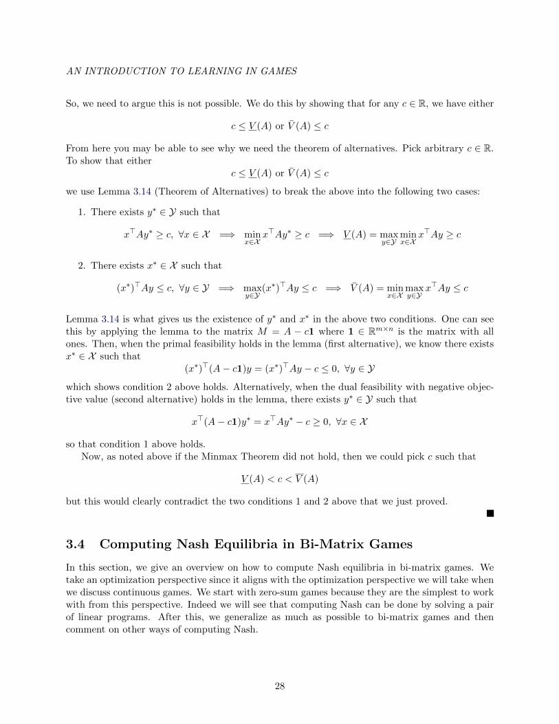
So, we need to argue this is not possible. We do this by showing that for any c ∈ R, we have either
c ≤ V (A) or V (A) ≤ c
From here you may be able to see why we need the theorem of alternatives. Pick arbitrary c ∈ R.To show that either
c ≤ V (A) or V (A) ≤ c
we use Lemma 3.14 (Theorem of Alternatives) to break the above into the following two cases:
1. There exists y∗ ∈ Y such that
x>Ay∗ ≥ c, ∀x ∈ X =⇒ minx∈X
x>Ay∗ ≥ c =⇒ V (A) = maxy∈Y
minx∈X
x>Ay ≥ c
2. There exists x∗ ∈ X such that
(x∗)>Ay ≤ c, ∀y ∈ Y =⇒ maxy∈Y
(x∗)>Ay ≤ c =⇒ V (A) = minx∈X
maxy∈Y
x>Ay ≤ c
Lemma 3.14 is what gives us the existence of y∗ and x∗ in the above two conditions. One can seethis by applying the lemma to the matrix M = A − c1 where 1 ∈ Rm×n is the matrix with allones. Then, when the primal feasibility holds in the lemma (first alternative), we know there existsx∗ ∈ X such that
(x∗)>(A− c1)y = (x∗)>Ay − c ≤ 0, ∀y ∈ Y
which shows condition 2 above holds. Alternatively, when the dual feasibility with negative objec-tive value (second alternative) holds in the lemma, there exists y∗ ∈ Y such that
x>(A− c1)y∗ = x>Ay∗ − c ≥ 0, ∀x ∈ X
so that condition 1 above holds.Now, as noted above if the Minmax Theorem did not hold, then we could pick c such that
V (A) < c < V (A)
but this would clearly contradict the two conditions 1 and 2 above that we just proved.
3.4 Computing Nash Equilibria in Bi-Matrix Games
In this section, we give an overview on how to compute Nash equilibria in bi-matrix games. Wetake an optimization perspective since it aligns with the optimization perspective we will take whenwe discuss continuous games. We start with zero-sum games because they are the simplest to workwith from this perspective. Indeed we will see that computing Nash can be done by solving a pairof linear programs. After this, we generalize as much as possible to bi-matrix games and thencomment on other ways of computing Nash.
28
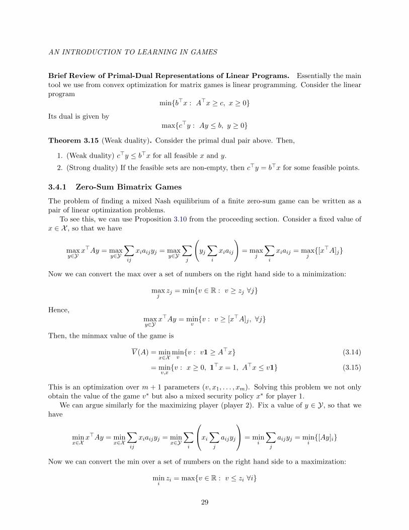
AN INTRODUCTION TO LEARNING IN GAMES
Brief Review of Primal-Dual Representations of Linear Programs. Essentially the maintool we use from convex optimization for matrix games is linear programming. Consider the linearprogram
minb>x : A>x ≥ c, x ≥ 0
Its dual is given bymaxc>y : Ay ≤ b, y ≥ 0
Theorem 3.15 (Weak duality). Consider the primal dual pair above. Then,
1. (Weak duality) c>y ≤ b>x for all feasible x and y.
2. (Strong duality) If the feasible sets are non-empty, then c>y = b>x for some feasible points.
3.4.1 Zero-Sum Bimatrix Games
The problem of finding a mixed Nash equilibrium of a finite zero-sum game can be written as apair of linear optimization problems.
To see this, we can use Proposition 3.10 from the proceeding section. Consider a fixed value ofx ∈ X , so that we have
maxy∈Y
x>Ay = maxy∈Y
∑ij
xiaijyj = maxy∈Y
∑j
(yj∑i
xiaij
)= max
j
∑i
xiaij = maxj[x>A]j
Now we can convert the max over a set of numbers on the right hand side to a minimization:
maxjzj = minv ∈ R : v ≥ zj ∀j
Hence,maxy∈Y
x>Ay = minvv : v ≥ [x>A]j , ∀j
Then, the minmax value of the game is
V (A) = minx∈X
minvv : v1 ≥ A>x (3.14)
= minv,xv : x ≥ 0, 1>x = 1, A>x ≤ v1 (3.15)
This is an optimization over m + 1 parameters (v, x1, . . . , xm). Solving this problem we not onlyobtain the value of the game v∗ but also a mixed security policy x∗ for player 1.
We can argue similarly for the maximizing player (player 2). Fix a value of y ∈ Y, so that wehave
minx∈X
x>Ay = minx∈X
∑ij
xiaijyj = minx∈Y
∑i
xi∑j
aijyj
= mini
∑j
aijyj = mini[Ay]i
Now we can convert the min over a set of numbers on the right hand side to a maximization:
minizi = maxv ∈ R : v ≤ zi ∀i
29
AN INTRODUCTION TO LEARNING IN GAMES
Hence,minx∈X
x>Ay = maxvv : v ≤ [Ay]i, ∀i
so that the maxmin value of the game is
V (A) = maxy∈Y
maxvv : v1 ≤ Ay (3.16)
= maxv,yv : y ≥ 0, 1>y = 1, Ay ≥ v1 (3.17)
Solving this problem we get the value of the game v∗ and a mixed security policy for player 2.These two problems we wrote down are in fact dual of one another, and by strong duality, we
have a solution x∗ = y∗. This is perhaps a surprising fact, that zero-sum games always have atleast one symmetric Nash equilibrium.
Now, if we want all the mixed security policies for each of the players we can use the value ofthe game to obtain this set:
x ∈ Rm| x ≥ 0, 1>x = 1, v∗1 ≥ A>x
andy ∈ Rn| y ≥ 0, 1>y = 1, v∗1 ≤ Ay
Linear programs can be solved in polynomial time (poly in m and n).
Seeing Minmax Theorem from Dual of the Dual. Let us now in a sense repeat what we haveseen above in a slightly different way that suggests that the maxmin problem is dual to the minmaxproblem and hence, for zero-sum games, strong duality gives the celebrated minmax theorem.
Mixed strategies x and y of the two players are nonnegative vectors whose components sum upto one. These conditions can be viewed as linear constraints:
X = 1>x = 1, x ≥ 0 and Y = 1>y = 1, y ≥ 0
Given a fixed y ∈ Y, a best response of player 1 to y is a vector x ∈ X that minimizes the expressionx>(Ay). That is, x is a solution to the linear program
minx>(Ay) : 1>x = 1, x ≥ 0 (3.18)
The dual of this linear program ismaxv : v1 ≤ Ay
Consider a zero-sum game G = (A,−A>). This minimum payoff to player 1 is the optimal valueof the linear program in (3.18), which is equal to the optimal value of v in its dual. Player 2 isinterested in maximizing v by their choice of y. The constraints of the dual are linear in v and yeven if y ∈ Y = y : 1>y = 1, y ≥ 0 is treated as the variable. Hence, a maxmin strategy y forplayer 2—i.e., maximizing the minimum amount they receive—is a solution to the linear programgiven by
maxv,yv : 1>y = 1, Ay − v1 ≥ 0, y ≥ 0 (3.19)
It is not hard to see that this linear program gives us a maxmin strategy for the y player.
30
AN INTRODUCTION TO LEARNING IN GAMES
Now, the dual of this linear program in (3.19) has variables x and u corresponding to the primalconstraints 1>y = 1 and Ay − v1 ≥ 0, respectively, and is given by
minu,xu : 1>x = 1, u1−A>x ≥ 0, x ≥ 0 (3.20)
This linear program gives us a minmax strategy for the x player, since they are minimizing themaximum amount they will pay.
Theorem 3.16 (von Neumann Min-Max via Duality [44]). A zero-sum cost minimization gameG = (A,−A>) has the equilibrium (x∗, y∗) if and only if (u∗, y∗) is an optimal solution to the linearprogram (3.19) and (v∗, x∗) is an optimal solution to its dual (3.20). Moverover, u∗ is the minmaxvalue of the game and v∗ is the maxmin value of the game such that u∗ = v∗.
It is also a very interesting fact that linear programs can be expressed as zero-sum games(cf. [1, 13]).
3.4.2 Computing Nash via Optimization in General Sum Bi-Matrix Games
Similar to the zero-sum case, finding Nash in bi-matrix general sum games can be approachedvia tools from optimization. In the next chapter, we will make a similar connection betweenoptimization and computation of Nash for continuous games. Such a formulation of equilibriumconditions as an optimization or feasibility problem can be used to infer agents’ utility functionsand can be used in constructing an an inverse formulation for designing feedback mechanisms toinduce a Nash equilibrium. It also leads to several natural learning dynamics which we will see inChapter 5. So this optimization framework is quite important.
Our focus will remain on two player matrix games since this allows us to introduce conceptsmore easily, however, it should be noted that many things we discuss can be extended in somemanner to network or polymatrix games, albeit with worse computational complexity.
Recall that the joint strategy space is the cross product of of the following two simplexes:x : x = (x1, . . . , xn),
∑i
xi = 1
×
y : y = (y1, . . . , ym),
∑i
yi = 1
= X × Y
Let us start by reasoning about points on the interior of X ×Y (inner or totally mixed strategies).Consider a cost minimization bi-matrix game G = (A,B). Let ai denote the rows of A and let
bj denote the columns of B>. Given a mixed strategy x ∈ X , we say that j ∈ X = 1, . . . ,m is inthe support of x if xj > 0. We use the notation supp(x) to denote the support—i.e.,
supp(x) = j ∈ X : xj > 0
Recall the best response notation: BRi(x−i) denotes player i’s best response map and it returnsthe set of strategies which are a best response to x−i. If a joint mixed strategy (x∗, y∗) is a Nashequilibrium, then for any j ∈ X
j ∈ BR1(y∗) ⇐⇒ x∗j > 0
since all pure strategies in the support of a Nash equilibrium strategy yields the same payoff orotherwise the player would have a strict preference for the pure strategy with the highest payoff.The gives us the following proposition.
31
AN INTRODUCTION TO LEARNING IN GAMES
Proposition 3.17. A point (x∗, y∗) is a Nash equilibrium of G = (A,B) if and only if every purestrategy in the support of x∗ is a best response to y∗. That is, (x∗, y∗) is a Nash equilibrium if andonly if for all pure strategies in (i, j) ∈ X × Y ,
xi > 0 =⇒ a>i y = min`∈X
a>` y (3.21)
yj > 0 =⇒ x>bj = min`∈Y
x>b` (3.22)
The above proposition essentially captures the fact that all pure strategies in the support ofa Nash equilibrium yield the same payoff which is also greater than or equal to the payoffs forstrategies outside the support. That is, for all j, k ∈ supp(x∗) we have
f1(j, y∗) = f1(k, y∗),
where f1(x, y) is player 1’s cost function and there is a slight abuse of notation in using j andk (pure strategies) to denote the mixed strategies that put all the probability mass on the j-th(respectively, k-th) entry of x. In addition, for all j ∈ supp(x∗) and ` /∈ supp(x∗), we have
f1(j, y∗) ≤ f1(`, y∗).
Similar conclusions can be drawn about player 2’s mixed Nash equilibrium strategy y∗. In otherwords, for purely mixed strategies (where the support set contains every pure strategy) we havethat
(x∗, y∗) is a Nash equilibrium ⇐⇒
a>1 y
∗ = a>i y∗ i = 2, . . . ,m
(x∗)>b1 = (x∗)>bj j = 2, . . . , n∑ni=1 xi = 1∑mj=1 yj = 1
This is a set of linear equations and can be solved efficiently.11
Not all games have purely mixed Nash strategies. Let us now formulation a naıve or brute forceextension of the purely mixed strategy computation strategy for cases where we do not have purelymixed strategies. A mixed strategy profile (x, y) ∈ X ×Y is a Nash equilibrium with supp(x) ⊆ Xand supp(y) ⊆ Y if and only if
u = aiy ∀ i ∈ supp(x)u ≥ aiy ∀ i /∈ supp(x)v = x>bj ∀ j ∈ supp(y)v ≥ x>bj ∀ j /∈ supp(y)xi = 0 ∀ i /∈ supp(x)yj = 0 ∀ j /∈ supp(y)
The issue with this computation method is that is requires finding the right support sets supp(x) andsupp(y). There are 2m+n different support sets; hence, this processes is exponential in computationtime.
11For games with more than 2 players, a similar line of reasoning leads to a set of polynomial equations.
32
AN INTRODUCTION TO LEARNING IN GAMES
An Optimization Approach
Instead of taking the approach of constructing the support sets (which works well for games withpurely mixed strategies, if we know a priori that such an equilibrium exists), we take an optimizationapproach. Indeed, this approach to finding equilibrium strategies for a bi-matrix game essentiallytransforms the problem into a nonlinear (in fact, a bilinear) programming problem.
Consider a general sum game G = (A,B). Observe that a best response of player 1 against amixed strategy y of player 2 is a solution to the linear program (3.18), which we recall here for easeof access:
minx>(Ay) : 1>x = 1, x ≥ 0
The dual of this linear program ismaxv : Ay ≥ v1
By strong duality, a feasible solution x is optimal if and only if there is a dual solution v fulfillingAy ≥ v1 and x>(Ay) = v—that is, x>(Ay) = x>1v which itself is equivalent to
x>(1v −Ay) = 0
Since the vectors x and 1v − Ay are both non-negative, the above equality says that they haveto be what is called complementary in that both cannot have positive components in the sameposition. This characterization of an optimal primal-dual pair of feasible solutions is known ascomplementary slackness in linear programming.
Since x has at least one positive component, the respective component of 1v −Ay is zero, andv is the maximum of the components of Ay. Indeed, any pure strategy i ∈ X is a best response toy if and only if the i-th component of the slack vector 1v−Ay is zero (since otherwise there wouldbe no mass on the strategy i in xi). This is saying that
[1v −Ay]i = 0 ⇐⇒ [xi > 0 =⇒ a>i y = max`∈X
a>` y]
Now, for player 2, y is a best response to x if and only if it minimizes (x>B>)y subject toy ∈ Y. The dual of this linear program is
maxu : Bx ≥ u1
A primal-dual pair (u, y) of feasible solutions is optimal if and only if
y>(1u−Bx) = 0
which is completely analogous to the complementarity problem discussed above for player 1.
Theorem 3.18. The cost minimization game G = (A,B) has the Nash equilibrium (x∗, y∗) if andonly if for some u, v the following hold:
1>y = 1, 1>x = 1, x ≥ 0, y ≥ 0 (3.23)
Ay − v1 ≥ 0 (3.24)
Bx− u1 ≥ 0 (3.25)
We can further introduce a cost to the above set of inequalities to get a bilinear optimizationproblem which has as solutions the Nash equilibria for the game.
33
AN INTRODUCTION TO LEARNING IN GAMES
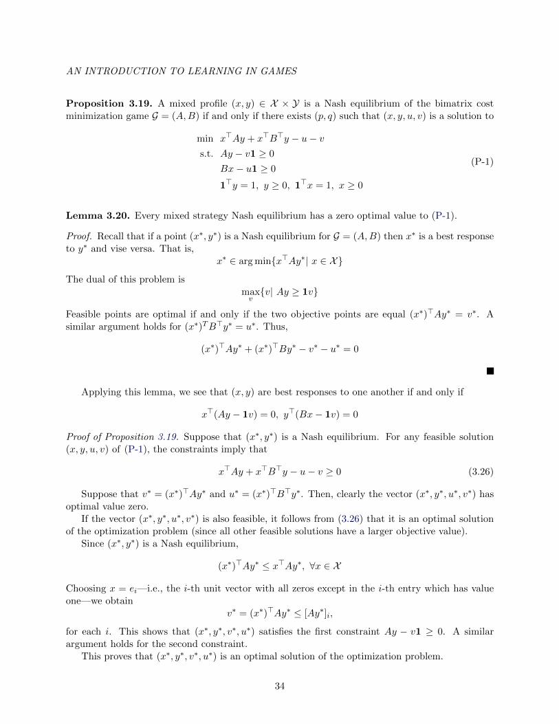
Proposition 3.19. A mixed profile (x, y) ∈ X × Y is a Nash equilibrium of the bimatrix costminimization game G = (A,B) if and only if there exists (p, q) such that (x, y, u, v) is a solution to
min x>Ay + x>B>y − u− vs.t. Ay − v1 ≥ 0
Bx− u1 ≥ 0
1>y = 1, y ≥ 0, 1>x = 1, x ≥ 0
(P-1)
Lemma 3.20. Every mixed strategy Nash equilibrium has a zero optimal value to (P-1).
Proof. Recall that if a point (x∗, y∗) is a Nash equilibrium for G = (A,B) then x∗ is a best responseto y∗ and vise versa. That is,
x∗ ∈ arg minx>Ay∗| x ∈ X
The dual of this problem ismaxvv| Ay ≥ 1v
Feasible points are optimal if and only if the two objective points are equal (x∗)>Ay∗ = v∗. Asimilar argument holds for (x∗)TB>y∗ = u∗. Thus,
(x∗)>Ay∗ + (x∗)>By∗ − v∗ − u∗ = 0
Applying this lemma, we see that (x, y) are best responses to one another if and only if
x>(Ay − 1v) = 0, y>(Bx− 1v) = 0
Proof of Proposition 3.19. Suppose that (x∗, y∗) is a Nash equilibrium. For any feasible solution(x, y, u, v) of (P-1), the constraints imply that
x>Ay + x>B>y − u− v ≥ 0 (3.26)
Suppose that v∗ = (x∗)>Ay∗ and u∗ = (x∗)>B>y∗. Then, clearly the vector (x∗, y∗, u∗, v∗) hasoptimal value zero.
If the vector (x∗, y∗, u∗, v∗) is also feasible, it follows from (3.26) that it is an optimal solutionof the optimization problem (since all other feasible solutions have a larger objective value).
Since (x∗, y∗) is a Nash equilibrium,
(x∗)>Ay∗ ≤ x>Ay∗, ∀x ∈ X
Choosing x = ei—i.e., the i-th unit vector with all zeros except in the i-th entry which has valueone—we obtain
v∗ = (x∗)>Ay∗ ≤ [Ay∗]i,
for each i. This shows that (x∗, y∗, v∗, u∗) satisfies the first constraint Ay − v1 ≥ 0. A similarargument holds for the second constraint.
This proves that (x∗, y∗, v∗, u∗) is an optimal solution of the optimization problem.
34
AN INTRODUCTION TO LEARNING IN GAMES
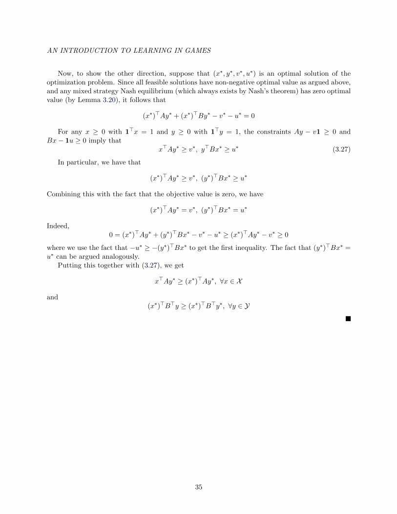
Now, to show the other direction, suppose that (x∗, y∗, v∗, u∗) is an optimal solution of theoptimization problem. Since all feasible solutions have non-negative optimal value as argued above,and any mixed strategy Nash equilibrium (which always exists by Nash’s theorem) has zero optimalvalue (by Lemma 3.20), it follows that
(x∗)>Ay∗ + (x∗)>By∗ − v∗ − u∗ = 0
For any x ≥ 0 with 1>x = 1 and y ≥ 0 with 1>y = 1, the constraints Ay − v1 ≥ 0 andBx− 1u ≥ 0 imply that
x>Ay∗ ≥ v∗, y>Bx∗ ≥ u∗ (3.27)
In particular, we have that
(x∗)>Ay∗ ≥ v∗, (y∗)>Bx∗ ≥ u∗
Combining this with the fact that the objective value is zero, we have
(x∗)>Ay∗ = v∗, (y∗)>Bx∗ = u∗
Indeed,0 = (x∗)>Ay∗ + (y∗)>Bx∗ − v∗ − u∗ ≥ (x∗)>Ay∗ − v∗ ≥ 0
where we use the fact that −u∗ ≥ −(y∗)>Bx∗ to get the first inequality. The fact that (y∗)>Bx∗ =u∗ can be argued analogously.
Putting this together with (3.27), we get
x>Ay∗ ≥ (x∗)>Ay∗, ∀x ∈ X
and(x∗)>B>y ≥ (x∗)>B>y∗, ∀y ∈ Y
35
Chapter 4
Games on Continuous Action Spaces
The second class of normal form games that we review are known as continuous games becauseplayers possess continuous action spaces.
Perhaps the most natural way to introduce continuous games is using finite games. Indeed,we can think of a normal form game on finite action spaces as a continuous game if we take intoconsideration mixed strategies. For instance, consider the bimatrix game (A,B)—i.e., f1(x1, x2) =x>1 Ax2 and f2(x1, x2) = x>2 Bx1. Mixed strategies for this game belong to the simplex ∆(X1) ×∆(X2)—that is, x1 ∈ ∆(X1) is a probability distribution on X1 such that each element in the vectorx1 = (x11, . . . , x1m1) takes on a value in the continuous interval [0, 1]. From this point of view, thegame (x>1 Ax2, x
>2 Bx1) can be viewed as a game on continuous actions spaces, albeit constrained
action spaces. In this way, mixed strategies over finite games can be thought of as pure strategiesin a continuous game over the simplex.
More generally, a game is called a continuous game if the strategy sets are topological spacesand the payoff functions are continuous with respect to the product topology. In particular, in con-tinuous games, players choose actions from a continuous action space, constrained or unconstrainedas it may be for the particular rules of the game. In particular, we consider games where playerschoose from a continuum and the utility/cost functions are continuous.
In the remainder of this chapter, we will introduce the Nash equilibrium concept and refinements(local Nash equilibria) as well as the Stackelberg equilibrium concept and refinements thereof. Wewill review different types of games including zero-sum, potential, convex, monotone and generalsum games. Existence results will be presented (largely without proof), and we will discuss how tocompute Nash equilibria taking an optimization approach as we did in the last chapter.
4.1 Nash Equilibrium Definition and Best Response
The definition of a (pure) Nash equilibrium does not change from what we saw for finite games.The only difference is that players’ actions are chosen from continuous action spaces.
Definition 4.1. A point x∗ is a Nash equilibrium for the continuous game (f1, . . . , fN ) if for eachi ∈ I
fi(x∗i , x∗−i) ≤ fi(xi, x∗−i) ∀ xi ∈ Xi
Best response are again useful for characterizing Nash as we have seen in Chapter 2. Towardsunderstanding the best response, we define the rational response set as follows. In an N–person
36
AN INTRODUCTION TO LEARNING IN GAMES
non-zero sum game, let the minimum of the cost function fi(x) of player i with respect to xi ∈ Xi
be attained for each x−i ∈ X−i Then, the set BRi(x−i) ⊂ Xi defined by
BRi(x−i) = ξ ∈ Xi : fi(xi, x−i) ≥ fi(ξ, x−i), ∀xi ∈ Xi
is called the best response set or rational reaction set for player i.
Definition 4.2. A point x∗ is a Nash equilibrium if x∗i ∈ BRi(x∗−i) for each i ∈ N .
Let’s consider a couple examples.
Example 4.3 (Simple Quadratic Game). Consider the game G = (f1, f2) where
f1(x, y) = (x− y)2 and f2(x, y) = (y − x)2
and x, y ∈ R. We claim that (x∗, y∗) = (0, 0) is a Nash equilibrium. Indeed,
f1(0, 0) = 0 ≤ f1(x, 0) = x2, ∀x ∈ R
andf2(0, 0) = 0 ≤ f2(0, y) = y2, ∀x ∈ R
The next example is one of two of the most quintessential continuous games, Cournot andBertrand Competition.
Example 4.4 (Cournot Game). In these games, players choose the quantity (respectively, price)of a product given competition for demand. Consider a scenario in which there are two firms. Theysimultaneously choose any quantity q1, q2 ≥ 0. The price in the market is given by p(q1, q2) =A− q1 − q2 for some constant A. The firms payoff functions are given by
ui(qi, q−i) = p(q1, q2)qi − ciq−i
for i = 1, 2. Consider the optimization problem that each player faces:
maxqiui(qi, q−i)| qi ≥ 0 (4.1)
Note that the utilities for each player are concave in their individual choice variables qi. Notice alsothere are constraints on the problem for each player but they are decoupled.1 So as in optimization,we will formulate the Lagrangian for each player:
Li(qi, q−i, µi) = ui(qi, q−i)− µ>i qi, µi ≥ 0 (4.2)
To calculate the equilibrium, we first find critical points of the Lagrangian functions for each playerholding the other player fixed. That is, we set their individual partial derivatives to zero as follows:
∂L1
∂q1= A− 2q1 − q2 − c1 − µ1 = 0
∂L2
∂q2= A− q1 − 2q2 − c2 − µ2 = 0
(4.3)
1When the constraints are coupled, things become a bit more complicated and we need to introduce the generalizedNash equilibrium concept. We will not do this in this course. We instead will deal with uncoupled constraints orvery well behaved constrained sets where things can be uncoupled through clever transformations.
37
AN INTRODUCTION TO LEARNING IN GAMES
Solving these two equations for q1, q2 in terms of µ1, µ2 and then using the fact that the Lagrangianfor each player is linear in µ1 and µ2, respectively, we have the following conditions:
q1 = 13(A+ c2 − 2c1) + 1
3(µ2 − 2µ1)
q2 = 13(A+ c1 − 2c2) + 1
3(µ1 − 2µ2)(4.4)
Now, we want to minimize the Lagrangian Li with respect to µi and it is linear in µi (i.e., the termin Li is −µiqi) and the original constraint is such that qi ≥ 0. Hence, µ∗i = 0 for each i = 1, 2. Thisgives us the best responses for each player:
q∗1 = 13(A+ c2 − 2c1)
q∗2 = 13(A+ c1 − 2c2)
(4.5)
The key point of this example, is that we can find the Nash equilibrium of the game by viewingthe problem as a set of coupled optimization problems. We took this similar view in how weformulated the optimization based approach for finding mixed Nash equilibria in bilinear matrixgames in the proceeding chapter. This motivates writing down necessary and sufficient conditionsfor Nash equilibria from this optimization perspective.
Both of the above examples are defined by cost functions that are strongly convex for each of theplayers. As we will see later this gives some assurances on not only existence but also uniqueness.When it is the case that the cost functions are not convex, we need local notions of equilibria. Fora metric space (X, d) with metric d, let Bδ(x) denote the ball of radius R centered at x.
Definition 4.5 (Local Nash Equilibrium). A point x∗ is a local Nash equilibrium for the continuousgame (f1, . . . , fN ) if for each i ∈ N , there exists a δi > 0 such that
fi(x∗i , x∗−i) ≤ fi(xi, x∗−i) ∀ xi ∈ Bδi(x
∗i ).
Another way local Nash are defined is as follows: given sets Ui ⊂ Xi for each i ∈ N , a point x∗
is a local Nash equilibrium on the set U = U1 × · · · × UN , if for each i ∈ N ,
fi(x∗i , x∗−i) ≤ fi(xi, x∗−i), ∀xi ∈ Ui.
4.2 An Optimization Approach to Nash in Unconstrained Games
We may consider using optimality conditions for each player’s individual optimization problem inorder to define refinements of the Nash equilibrium concept, and to guide how we may computesuch refinements.
Suppose that Xi ⊂ Rmi for each i and let
X = X1 × · · · ×Xn
Here, we will only concern ourselves with full information games and reduce the notation for agame to be the tuple
G = (f1, . . . , fN )
where each fi ∈ C2(X,R). Consider the unconstrained optimization problem for player i:
minxi∈Rmi
fi(xi, x−i) (4.6)
Holding x−i ∈ Rm−mi fixed, we can view this simply as an optimization problem in the variable xi.
38
AN INTRODUCTION TO LEARNING IN GAMES
A little foray back to calculus. We know from calculus (and nonlinear programming) whatthe necessary and sufficient optimality conditions are for a extremal point. Recall the definition ofa global minima of a (sufficiently smooth) function h(x).
Definition 4.6. A point x∗ ∈ X is a global minima of h(x) if
h(x∗) ≤ h(x), ∀ x ∈ X
Since h(x) might in general be non-convex in x, we also recall the definition of a local minima.
Definition 4.7. A point x∗ ∈ X is a local minima of h(x) if there exists a δ > 0 such that
h(x∗) ≤ h(x), ∀ x ∈ Bδ(x∗)
Moreover, we say that x∗ is a local minimum on the set U if the above inequality holds for allx ∈ U .
We know from calculus that a point x∗ ∈ Rm is a local minimum of
minx∈Rm
h(x)
if the following sufficient conditions hold:
1. First order conditions:Dh(x∗) = 0 (4.7)
2. Second order conditions:D2h(x∗) > 0 (4.8)
On the other hand, if x∗ is a local minimum, then necessarily Dh(x∗) = 0 and Dh(x∗) ≥ 0.Importantly, it is a generic property of C2-functions that all local minima satisfy conditions
(4.7) and (4.8) above. This is true not only on Euclidean space but also for sufficiently smoothfunctions on smooth manifolds (without boundary). Formally, this means that set of functionsfor which the sufficient conditions above are not also necessary is of measure zero in the class ofC2(Rm,R) functions.
Coming back to games. Now, let us return to the game setting. First, since fi(xi, x−i) mayalso be, in general, non-convex in xi, we focus on the local Nash equilibrium concept. Recall theoptimization problem in (4.6) where we consider for a moment that x−i ∈ Rm−mi is fixed. Then thisoptimization problem over xi ∈ Rm is exactly of the form discussed above and hence, we can writedown optimality conditions for each player. Indeed, given x∗−i ∈ Rm−mi , x∗i is a local minimum ifthe following sufficient conditions hold:
1. Difi(x∗i , x∗−i) = 0
2. D2i fi(x
∗i , x∗−i) > 0
These individual derivatives Difi(x) are the directions in which a player i can make ”differential”adjustments to its strategy in order to improve the cost locally as indicated by the individual cur-vature D2
i fi(x). This observation leads to the following definition of a differential Nash equilibrium.
39
AN INTRODUCTION TO LEARNING IN GAMES
Definition 4.8 (Ratliff, Burden, Sastry, 2013 [45]2). A strategy x = (x1, . . . , xN ) is a differentialNash equilbrium of the game G = (f1, . . . , fN ) if Difi(x) = 0 and D2
i fi(x) > 0 for each i ∈ N .
The definition of a differential Nash equilibrium is inherently local. Furthermore, differentialNash equilibria are clearly strict local Nash equilibria.
Proposition 4.9 (Ratliff, Burden, Sastry, 2013 [45]). A differential Nash equilibrium of the gameG = (f1, . . . , fN ) is a strict local Nash equilibrium.
The conditions of the definition are sufficient for checking if a point is a Nash equilibrium. Theselook just like first and second order conditions for optimality, but they are not necessary.
Example 4.10. Consider the zero sum game G = (f,−f) defined by f(x1, x2) = x>1 x2. Then,(x1, x2) = (0, 0) is a local Nash equilibrium since
f(0, 0) = 0 ≤ x>1 0 = 0, ∀x1 ∈ Rm1
and−f(0, 0) = 0 ≤ −0>x2 = 0, ∀x2 ∈ Rm2
Yet, following the same construction of necessary conditions for local minima, we can writedown necessary conditions for local Nash equilibria.
Proposition 4.11 (Ratliff, Burden, Sastry, 2013 [45]). Suppose x∗ is a local Nash equilibrium ofthe game G = (f1, . . . , fN ). Then, Difi(x
∗) = 0 and D2i fi(x
∗) ≥ 0.
One very interesting observation is that unlike strict local minima in single player optimization,a point being a strict local Nash (differential Nash) equilibrium is not sufficient to guarantee thatit is isolated. Indeed, it is is easy to construct examples with a continuum of differential Nashequilibria.
Example 4.12 (Continuum of Differential Nash Equlibria.). Consider the game G = (f1, f2)defined by the following cost functions:
f1(x1, x2) = 12x
21 − x1x2
f2(x1, x2) = 12x
22 − x1x2
(4.9)
Every point on the line x1 = x2 is a differential Nash equilibrium. Indeed,
D1f1(x) = x1 − x2 = 0, D2f2(x1, x2) = x2 − x1 = 0 ⇐⇒ x1 = x2
andD2
1f1(x) = D22f2(x) = 1 > 0, ∀x
To see these points are local Nash, observe that for any x1 = x2 = y, we have
f1(y, y) =1
2y2 − y2 = −1
2y2 < x2
1 − x1y, ∀x1 6= y
2Note this definition can be extended to a well-defined differential form in settings where the strategy spaces ofagents are manifolds (without boundary)
40
AN INTRODUCTION TO LEARNING IN GAMES
and similarly,
f2(y, y) =1
2y2 − y2 = −1
2y2 < x2
2 − x2y, ∀x2 6= y
This continuum of equilibria is not robust however. That is, even small changes to the game willremove the continuum. Indeed, consider the game
f1(x1, x2) = 12x
21 − εx1x2
f2(x1, x2) = 12x
22 − x1x2
(4.10)
defined for some arbitrary ε 6= 1. Then,
D1f1(x) = x1 − εx2 = 0, D2f2(x) = −x1 + x2 = 0 ⇐⇒ x1 = x2 = 0
That is, the only candidate local Nash equilibrium is now at x∗ = (0, 0). We can check that it is infact a Nash equilibrium by check the second order sufficient conditions:
D21f1(x∗) = 1 > 0, D2
2f2(x∗) = 1 > 0
This shows that all the differential Nash on the line x1 = x2 disappear except the one at the origin.
To rule out a continuum of equilibria, we can check that the game Jacobian, which is given by
J(x) = Dg(x) =
[D2
1f1(x) D12f1(x)D21f2(x) D2
2f2(x)
]and is the derivative of the vector g(x) = (D1f1(x), D2f2(x))), is non-degenerate at critical pointsx∗—i.e., det(J(x∗)) 6= 0. Analogous to the case of single player optimization, non-degeneratedifferential Nash equilibria are generic amongst local Nash equilibria. That is, for all but a measurezero set of games (in the space of games defined by C2(X,R) functions), local Nash equilibria arenon-degenerate differential Nash equilibria.
4.3 Types of Games
There are many classes of games, most categorized by the structure of the cost function. In thissection, we will discuss two key types of games.
4.3.1 Potential and Zero-Sum (Hamiltonian) Games
Let’s start with the Jacobian of the previous section. This will help us define two important typesof games.
For simplicity, let’s again consider two players. Recall that the game Jacobian—i.e., the Ja-cobain of g(x) = (D1f1(x1, x2), D2f2(x1, x2))—is given by
J(x) = Dg(x) =
[D2
1f1(x) D12f1(x)D21f2(x) D2
2f2(x)
](4.11)
41
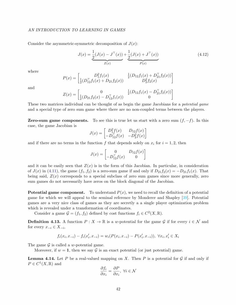
AN INTRODUCTION TO LEARNING IN GAMES
Consider the asymmetric-symmetric decomposition of J(x):
J(x) =1
2(J(x)− J>(x))︸ ︷︷ ︸
Z(x)
+1
2(J(x) + J>(x))︸ ︷︷ ︸
P (x)
(4.12)
where
P (x) =
[D2
1f1(x) 12(D12f1(x) +D>21f2(x))
12(D>12f1(x) +D21f2(x)) D2
2f2(x)
]and
Z(x) =
[0 1
2(D12f1(x)−D>21f2(x))12(D21f2(x)−D>12f1(x)) 0
]These two matrices individual can be thought of as begin the game Jacobians for a potential gameand a special type of zero sum game where there are no non-coupled terms between the players.
Zero-sum game components. To see this is true let us start with a zero sum (f,−f). In thiscase, the game Jacobian is
J(x) =
[D2
1f(x) D12f(x)−D>12f(x) −D2
2f(x)
]and if there are no terms in the function f that depends solely on xi for i = 1, 2, then
J(x) =
[0 D12f(x)
−D>12f(x) 0
]and it can be easily seen that Z(x) is in the form of this Jacobian. In particular, in considerationof J(x) in (4.11), the game (f1, f2) is a zero-sum game if and only if D21f2(x) = −D21f1(x). Thatbeing said, Z(x) corresponds to a special subclass of zero sum games since more generally, zerosum games do not necessarily have zeros on the block diagonal of the Jacobian.
Potential game component. To understand P (x), we need to recall the definition of a potentialgame for which we will appeal to the seminal reference by Monderer and Shapley [39]. Potentialgames are a very nice class of games as they are secretly a a single player optimization problemwhich is revealed under a transformation of coordinates.
Consider a game G = (f1, f2) defined by cost functions fi ∈ C2(X,R).
Definition 4.13. A function P : X → R is a w-potential for the game G if for every i ∈ N andfor every x−i ∈ X−i,
fi(xi, x−i)− fi(x′i, x−i) = wi(P (xi, x−i)− P (x′i, x−i)), ∀xi, x′i ∈ Xi
The game G is called a w-potential game.Moreover, if w = 1, then we say G is an exact potential (or just potential) game.
Lemma 4.14. Let P be a real-valued mapping on X. Then P is a potential for G if and only ifP ∈ C1(X,R) and
∂fi∂xi
=∂P
∂xi, ∀i ∈ N
42
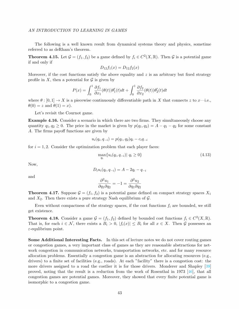
AN INTRODUCTION TO LEARNING IN GAMES
The following is a well known result from dynamical systems theory and physics, sometimereferred to as deRham’s theorem.
Theorem 4.15. Let G = (f1, f2) be a game defined by fi ∈ C2(X,R). Then G is a potential gameif and only if
D12f1(x) = D12f2(x)
Moreover, if the cost functions satisfy the above equality and z is an arbitrary but fixed strategyprofile in X, then a potential for G is given by
P (x) =
∫ 1
0
∂f1
∂x1(θ(t))θ′1(t)dt+
∫ 1
0
∂f2
∂x2(θ(t))θ′2(t)dt
where θ : [0, 1]→ X is a piecewise continuously differentiable path in X that connects z to x—i.e.,θ(0) = z and θ(1) = x).
Let’s revisit the Cournot game.
Example 4.16. Consider a scenario in which there are two firms. They simultaneously choose anyquantity q1, q2 ≥ 0. The price in the market is given by p(q1, q2) = A − q1 − q2 for some constantA. The firms payoff functions are given by
ui(qi, q−i) = p(q1, q2)qi − ciq−i
for i = 1, 2. Consider the optimization problem that each player faces:
maxqiui(qi, q−i)| qi ≥ 0 (4.13)
Now,Diui(qi, q−i) = A− 2qi − q−i
and∂2u1
∂q1∂q2= −1 =
∂2u2
∂q1∂q2
Theorem 4.17. Suppose G = (f1, f2) is a potential game defined on compact strategy spaces X1
and X2. Then there exists a pure strategy Nash equilibrium of G.
Even without compactness of the strategy spaces, if the cost functions fi are bounded, we stillget existence.
Theorem 4.18. Consider a game G = (f1, f2) defined by bounded cost functions fi ∈ C2(X,R).That is, for each i ∈ N , there exists a Bi > 0, |fi(x)| ≤ Bi for all x ∈ X. Then G possesses anε-equlibrium point.
Some Additional Interesting Facts. In this set of lecture notes we do not cover routing gamesor congestion games, a very important class of games as they are reasonable abstractions for net-work congestion in communication networks, transportation networks, etc. and for many resourceallocation problems. Essentially a congestion game is an abstraction for allocating resources (e.g.,drivers) to a finite set of facilities (e.g., roads). At each ”facility” there is a congestion cost: themore drivers assigned to a road the costlier it is for those drivers. Monderer and Shapley [39]proved, noting that the result is a reduction from the work of Rosenthal in 1973 [46], that allcongestion games are potential games. Moreover, they showed that every finite potential game isisomorphic to a congestion game.
43
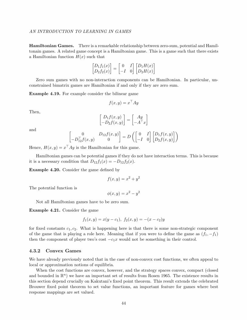
AN INTRODUCTION TO LEARNING IN GAMES
Hamiltonian Games. There is a remarkable relationship between zero-sum, potential and Hamil-tonain games. A related game concept is a Hamiltonian game. This is a game such that there existsa Hamiltonian function H(x) such that[
D1f1(x)D2f2(x)
]=
[0 I−I 0
] [D1H(x)D2H(x)
]Zero sum games with no non-interaction components can be Hamiltonian. In particular, un-
constrained bimatrix games are Hamiltonian if and only if they are zero sum.
Example 4.19. For example consider the bilinear game
f(x, y) = x>Ay
Then, [D1f(x, y)−D2f(x, y)
]=
[Ay−A>x
]and [
0 D12f(x, y)−D>12f(x, y) 0
]= D
([0 I−I 0
] [D1f(x, y)D2f(x, y)
])Hence, H(x, y) = x>Ay is the Hamiltonian for this game.
Hamiltonian games can be potential games if they do not have interaction terms. This is becauseit is a necessary condition that D12f1(x) = −D12f2(x).
Example 4.20. Consider the game defined by
f(x, y) = x2 + y2
The potential function isφ(x, y) = x2 − y2
Not all Hamiltonian games have to be zero sum.
Example 4.21. Consider the game
f1(x, y) = x(y − c1), f2(x, y) = −(x− c2)y
for fixed constants c1, c2. What is happening here is that there is some non-strategic componentof the game that is playing a role here. Meaning that if you were to define the game as (f1,−f1)then the component of player two’s cost −c1x would not be something in their control.
4.3.2 Convex Games
We have already previously noted that in the case of non-convex cost functions, we often appeal tolocal or approximation notions of equilibria.
When the cost functions are convex, however, and the strategy spaces convex, compact (closedand bounded in Rn) we have an important set of results from Rosen 1965. The existence results inthis section depend crucially on Kakutani’s fixed point theorem. This result extends the celebratedBrouwer fixed point theorem to set value functions, an important feature for games where bestresponse mappings are set valued.
44
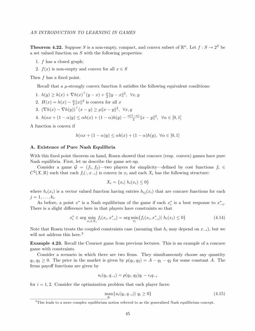
AN INTRODUCTION TO LEARNING IN GAMES
Theorem 4.22. Suppose S is a non-empty, compact, and convex subset of Rn. Let f : S → 2S bea set valued function on S with the following properties:
1. f has a closed graph;
2. f(x) is non-empty and convex for all x ∈ S
Then f has a fixed point.
Recall that a µ-strongly convex function h satisfies the following equivalent conditions:
1. h(y) ≥ h(x) +∇h(x)>(y − x) + µ2‖y − x‖
2, ∀x, y2. H(x) = h(x)− µ
2‖x‖2 is convex for all x
3. (∇h(x)−∇h(y))>(x− y) ≥ µ‖x− y‖2, ∀x, y
4. h(αx+ (1− α)y) ≤ αh(x) + (1− α)h(y)− α(1−α)2 ‖x− y‖2, ∀α ∈ [0, 1]
A function is convex if
h(αx+ (1− α)y) ≤ αh(x) + (1− α)h(y), ∀α ∈ [0, 1]
A. Existence of Pure Nash Equilibria
With this fixed point theorem on hand, Rosen showed that concave (resp. convex) games have pureNash equilibria. First, let us describe the game set-up.
Consider a game G = (f1, f2)—two players for simplicity—defined by cost functions fi ∈C2(X,R) such that each fi(·, x−i) is convex in xi and each Xi has the following structure:
Xi = xi| hi(xi) ≤ 0
where hi(xi) is a vector valued function having entries hij(xi) that are concave functions for eachj = 1, . . . , ki.
As before, a point x∗ is a Nash equilibrium of the game if each x∗i is a best response to x∗−i.There is a slight difference here in that players have constraints so that
x∗i ∈ arg minxi∈Xi
fi(xi, x∗−i) = arg min
xifi(xi, x∗−i)| hi(xi) ≤ 0 (4.14)
Note that Rosen treats the coupled constraints case (meaning that hi may depend on x−i), but wewill not address this here.3
Example 4.23. Recall the Cournot game from previous lectures. This is an example of a concavegame with constraints.
Consider a scenario in which there are two firms. They simultaneously choose any quantityq1, q2 ≥ 0. The price in the market is given by p(q1, q2) = A − q1 − q2 for some constant A. Thefirms payoff functions are given by
ui(qi, q−i) = p(q1, q2)qi − ciq−i
for i = 1, 2. Consider the optimization problem that each player faces:
maxqiui(qi, q−i)| qi ≥ 0 (4.15)
3This leads to a more complex equilibrium notion referred to as the generalized Nash equilibrium concept.
45
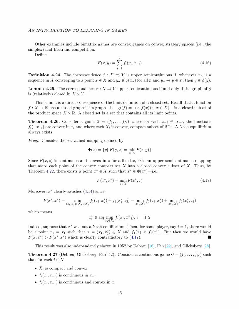
AN INTRODUCTION TO LEARNING IN GAMES
Other examples include bimatrix games are convex games on convex strategy spaces (i.e., thesimplex) and Bertrand competition.
Define
F (x, y) =2∑i=1
fi(yi, x−i) (4.16)
Definition 4.24. The correspondence φ : X ⇒ Y is upper semicontinuous if, whenever xn is asequence in X converging to a point x ∈ X and yn ∈ φ(xn) for all n and yn → y ∈ Y , then y ∈ φ(y).
Lemma 4.25. The correspondence φ : X ⇒ Y upper semicontinuous if and only if the graph of φis (relatively) closed in X × Y .
This lemma is a direct consequence of the limit definition of a closed set. Recall that a functionf : X → R has a closed graph if its graph—i.e. gr(f) = (x, f(x)) : x ∈ X—is a closed subset ofthe product space X × R. A closed set is a set that contains all its limit points.
Theorem 4.26. Consider a game G = (f1, . . . , fN ) where for each x−i ∈ X−i, the functionsfi(·, x−i) are convex in xi and where each Xi is convex, compact subset of Rmi . A Nash equilibriumalways exists.
Proof. Consider the set-valued mapping defined by
Φ(x) = y| F (y, x) = minz∈X
F (z, y)
Since F (x, z) is continuous and convex in z for a fixed x, Φ is an upper semicontinuous mappingthat maps each point of the convex compact set X into a closed convex subset of X. Thus, byTheorem 4.22, there exists a point x∗ ∈ X such that x∗ ∈ Φ(x∗)—i.e.,
F (x∗, x∗) = minz∈X
F (x∗, z) (4.17)
Moreover, x∗ clearly satisfies (4.14) since
F (x∗, x∗) = min(z1,z2)∈X1×X2
f1(z1, x∗2) + f2(x∗1, z2) = min
z1∈X1
f1(z1, x∗2) + min
z2∈X2
f2(x∗1, z2)
which meansx∗i ∈ arg min
xi∈Xifi(xi, x
∗−i), i = 1, 2
Indeed, suppose that x∗ was not a Nash equilibrium. Then, for some player, say i = 1, there wouldbe a point x1 = x1 such that x = (x1, x
∗2) ∈ X and f1(x) < f1(x∗). But then we would have
F (x, x∗) > F (x∗, x∗) which is clearly contradictory to (4.17).
This result was also independently shown in 1952 by Debreu [16], Fan [22], and Glicksberg [28].
Theorem 4.27 (Debreu, Glicksberg, Fan ’52). Consider a continuous game G = (f1, . . . , fN ) suchthat for each i ∈ N
• Xi is compact and convex
• fi(xi, x−i) is continuous in x−i
• fi(xi, x−i) is continuous and convex in xi
46
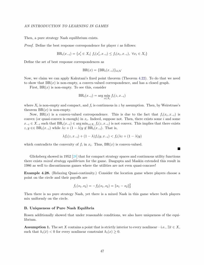
AN INTRODUCTION TO LEARNING IN GAMES
Then, a pure strategy Nash equilibrium exists.
Proof. Define the best response correspondence for player i as follows:
BRi(x−i) = x′i ∈ Xi| fi(x′i, x−i) ≤ fi(xi, x−i), ∀xi ∈ Xi
Define the set of best response correspondences as
BR(x) = BRi(x−i)i∈N
Now, we claim we can apply Kakutani’s fixed point theorem (Theorem 4.22). To do that we needto show that BR(x) is non-empty, a convex-valued correspondence, and has a closed graph.
First, BR(x) is non-empty. To see this, consider
BRi(x−i) = arg minz∈Xi
fi(z, x−i)
where Xi is non-empty and compact, and fi is continuous in z by assumption. Then, by Weirstrass’stheorem BR(x) is non-empty.
Now, BR(x) is a convex-valued correspondence. This is due to the fact that fi(xi, x−i) isconvex (or quasi-convex is enough) in xi. Indeed, suppose not. Then, there exists some i and somex−i ∈ X−i such that BRi(x−i) ∈ arg minz∈Xi fi(z, x−i) is not convex. This implies that there existsz, y ∈∈ BRi(x−i) while λz + (1− λ)y 6∈ BRi(x−i). That is,
λfi(z, x−i) + (1− λ)fi(y, x−i) < fi(λz + (1− λ)y)
which contradicts the convexity of fi in xi. Thus, BR(x) is convex-valued.
Glicksberg showed in 1952 [28] that for compact strategy spaces and continuous utility functionsthere exists mixed strategy equilibrium for the game. Dasgupta and Maskin extended this result in1986 as well to discontinuous games where the utilities are not even quasi-concave!
Example 4.28. (Relaxing Quasi-continuity.) Consider the location game where players choose apoint on the circle and their payoffs are
f1(s1, s2) = −f2(s1, s2) = ‖s1 − s2‖22
Then there is no pure strategy Nash, yet there is a mixed Nash in this game where both playersmix uniformly on the circle.
B. Uniqueness of Pure Nash Equlibria
Rosen additionally showed that under reasonable conditions, we also have uniqueness of the equi-librium.
Assumption 1. The setX contains a point that is strictly interior to every nonlinear—i.e., ∃x ∈ X,such that hi(x) < 0 for every nonlinear constraint hi(x) ≥ 0.
47
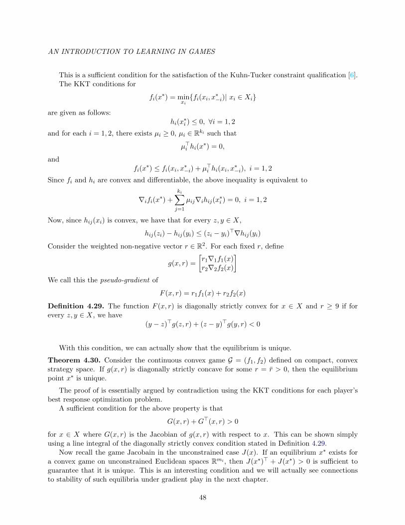
AN INTRODUCTION TO LEARNING IN GAMES
This is a sufficient condition for the satisfaction of the Kuhn-Tucker constraint qualification [6].The KKT conditions for
fi(x∗) = min
xifi(xi, x∗−i)| xi ∈ Xi
are given as follows:hi(x
∗i ) ≤ 0, ∀i = 1, 2
and for each i = 1, 2, there exists µi ≥ 0, µi ∈ Rki such that
µ>i hi(x∗) = 0,
andfi(x
∗) ≤ fi(xi, x∗−i) + µ>i hi(xi, x∗−i), i = 1, 2
Since fi and hi are convex and differentiable, the above inequality is equivalent to
∇ifi(x∗) +
ki∑j=1
µij∇ihij(x∗i ) = 0, i = 1, 2
Now, since hij(xi) is convex, we have that for every z, y ∈ X,
hij(zi)− hij(yi) ≤ (zi − yi)>∇hij(yi)
Consider the weighted non-negative vector r ∈ R2. For each fixed r, define
g(x, r) =
[r1∇1f1(x)r2∇2f2(x)
]We call this the pseudo-gradient of
F (x, r) = r1f1(x) + r2f2(x)
Definition 4.29. The function F (x, r) is diagonally strictly convex for x ∈ X and r ≥ 9 if forevery z, y ∈ X, we have
(y − z)>g(z, r) + (z − y)>g(y, r) < 0
With this condition, we can actually show that the equilibrium is unique.
Theorem 4.30. Consider the continuous convex game G = (f1, f2) defined on compact, convexstrategy space. If g(x, r) is diagonally strictly concave for some r = r > 0, then the equilibriumpoint x∗ is unique.
The proof of is essentially argued by contradiction using the KKT conditions for each player’sbest response optimization problem.
A sufficient condition for the above property is that
G(x, r) +G>(x, r) > 0
for x ∈ X where G(x, r) is the Jacobian of g(x, r) with respect to x. This can be shown simplyusing a line integral of the diagonally strictly convex condition stated in Definition 4.29.
Now recall the game Jacobain in the unconstrained case J(x). If an equilibrium x∗ exists fora convex game on unconstrained Euclidean spaces Rmi , then J(x∗)> + J(x∗) > 0 is sufficient toguarantee that it is unique. This is an interesting condition and we will actually see connectionsto stability of such equilibria under gradient play in the next chapter.
48
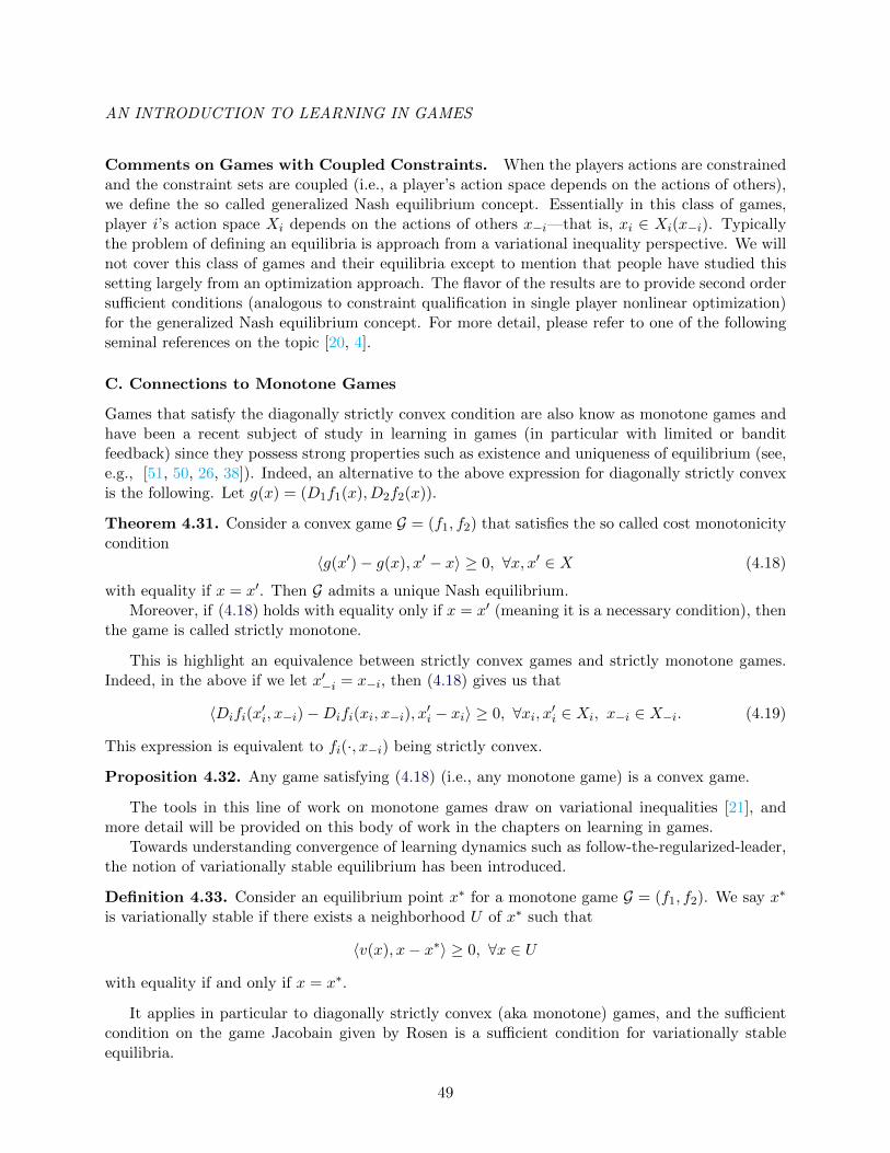
AN INTRODUCTION TO LEARNING IN GAMES
Comments on Games with Coupled Constraints. When the players actions are constrainedand the constraint sets are coupled (i.e., a player’s action space depends on the actions of others),we define the so called generalized Nash equilibrium concept. Essentially in this class of games,player i’s action space Xi depends on the actions of others x−i—that is, xi ∈ Xi(x−i). Typicallythe problem of defining an equilibria is approach from a variational inequality perspective. We willnot cover this class of games and their equilibria except to mention that people have studied thissetting largely from an optimization approach. The flavor of the results are to provide second ordersufficient conditions (analogous to constraint qualification in single player nonlinear optimization)for the generalized Nash equilibrium concept. For more detail, please refer to one of the followingseminal references on the topic [20, 4].
C. Connections to Monotone Games
Games that satisfy the diagonally strictly convex condition are also know as monotone games andhave been a recent subject of study in learning in games (in particular with limited or banditfeedback) since they possess strong properties such as existence and uniqueness of equilibrium (see,e.g., [51, 50, 26, 38]). Indeed, an alternative to the above expression for diagonally strictly convexis the following. Let g(x) = (D1f1(x), D2f2(x)).
Theorem 4.31. Consider a convex game G = (f1, f2) that satisfies the so called cost monotonicitycondition
〈g(x′)− g(x), x′ − x〉 ≥ 0, ∀x, x′ ∈ X (4.18)
with equality if x = x′. Then G admits a unique Nash equilibrium.Moreover, if (4.18) holds with equality only if x = x′ (meaning it is a necessary condition), then
the game is called strictly monotone.
This is highlight an equivalence between strictly convex games and strictly monotone games.Indeed, in the above if we let x′−i = x−i, then (4.18) gives us that
〈Difi(x′i, x−i)−Difi(xi, x−i), x
′i − xi〉 ≥ 0, ∀xi, x′i ∈ Xi, x−i ∈ X−i. (4.19)
This expression is equivalent to fi(·, x−i) being strictly convex.
Proposition 4.32. Any game satisfying (4.18) (i.e., any monotone game) is a convex game.
The tools in this line of work on monotone games draw on variational inequalities [21], andmore detail will be provided on this body of work in the chapters on learning in games.
Towards understanding convergence of learning dynamics such as follow-the-regularized-leader,the notion of variationally stable equilibrium has been introduced.
Definition 4.33. Consider an equilibrium point x∗ for a monotone game G = (f1, f2). We say x∗
is variationally stable if there exists a neighborhood U of x∗ such that
〈v(x), x− x∗〉 ≥ 0, ∀x ∈ U
with equality if and only if x = x∗.
It applies in particular to diagonally strictly convex (aka monotone) games, and the sufficientcondition on the game Jacobain given by Rosen is a sufficient condition for variationally stableequilibria.
49
AN INTRODUCTION TO LEARNING IN GAMES
4.3.3 Non-Convex Games
The most general type of game we will consider are games defined by non-convex cost functions. Asnoted before, analogous to the non-convex single player optimization case, since the cost functionsare non-convex we need local notions of equilibria, the definition of which we recall here for ease ofaccess.
Definition 4.34 (Local Nash Equilibrium). A point x∗ is a local Nash equilibrium on U1×U2 forthe continuous game (f1, . . . , fN ) if for each i ∈ 1, 2,
fi(x∗i , x∗−i) ≤ fi(xi, x∗−i) ∀ xi ∈ Ui.
Nash equilibria in non-convex games are NP-hard to compute in general, even in zero-sumsettings where there is a lot of structure. Some efforts have been put forth to better understandthe complexity in different settings [33, 15]. It is a highly active area of research to define newrefinements of Nash equilibria that ensure existence but also are game theoretically meaningful [35,23, 32]. Motivated by the use of minmax formulations in machine learning and reinforcementlearning, the focus over the last couple years has been primarily on zero-sum settings.
Let’s focus our attention on zero-sum settings where we will connect minmax problems, includingtheir equilibrium notions, to games.
A. Zero-sum Non-convex Games
Consider the following minmax optimization problem:
minx∈X
maxy∈Y
f(x, y) (4.20)
We can similarly think about the corresponding zero sum game G = (f,−f) in which the playersface the following best response problems:
minx∈X
f(x, y) (4.21)
maxy∈Y
f(x, y) (4.22)
Recall that in the previous chapter on finite games, we saw the celebrated minmax theorem whichstates that
minx∈X
maxy∈Y
f(x, y) = maxy∈Y
minx∈X
f(x, y)
This theorem also holds more generally when the cost function f is convex-concave (i.e., convex inx and concave in y). A word of caution however: in the nonconvex setting
minx∈X
maxy∈Y
f(x, y) 6= maxy∈Y
minx∈X
f(x, y)
in general.Because of this, there has been a surge of recent work connecting minmax and maxmin equilibria
to Nash equilibria (i.e., points where the maxmin and minmax values are equal). With non-convexities in mind, there are a number of local equilibrium concepts for minmax problems includinglocal Nash.
50
AN INTRODUCTION TO LEARNING IN GAMES
Stackelberg Formulations of Minmax Problems. In recent work by Fiez et al., the notionof a local Stackelberg equilibrium was introduced in the context of learning in continuous games.
In a Stackelberg game, the leader and follower aim to solve the following optimization problems,respectively:
minx1∈X1
f1(x1, x2)∣∣ x2 ∈ arg min
y∈X2
f2(x1, y), ( L)
minx2∈X2
f2(x1, x2). ( F)
This contrasts with a simultaneous play game in which each player i is faced with the optimizationproblem minxi∈Xi fi(xi, x−i).
Definition 4.35 (Fiez et al. [23] Local Stackleberg). Consider Ui ⊂ Xi for each i ∈ 1, 2. Thestrategy x∗1 ∈ U1 is a local Stackelberg solution for the leader if, ∀x1 ∈ U1,
supx2∈RU2(x∗1) f(x∗1, x2) ≤ supx2∈RU2
(x1) f(x1, x2),
where RU2(x1) = y ∈ U2| − f(x1, y) ≤ −f(x1, x2),∀x2 ∈ U2. Moreover, (x∗1, x∗2) for any x∗2 ∈
RU2(x∗1) is a local Stackelberg equilibrium on U1 × U2.
Note that this definition is not restricted to zero-sum settings. Indeed, replacing −f with f2
and f with f , the definition holds for the general sum game (f1, f2). This is one of the benefits ofthe Stackelberg formulation versus some of the other notions we consider in this section.
Analogous to the differential Nash notion we saw earlier in the chapter, there is also a differentialStackelberg equilibrium concept.
Definition 4.36 (Differential Stackelberg [23]). The joint strategy x∗ = (x∗1, x∗2) ∈ X is a differ-
ential Stackelberg equilibrium if Df1(x∗) = 0, D2f2(x∗) = 0, D2f1(x∗) > 0, and D22f2(x∗) > 0.
Classical Local Minmax Equilibrium Concepts.
Definition 4.37 (Evtushenko [17, 18] Local MinMax). A point (x∗, y∗) is a Evtushenko localminmax equilibrium if
f(x∗, y) ≤ f(x∗, y∗) ≤ f(x, y(x))
where y(x) ∈ y(x) with
y(x) =
y : max
y∈Yf(x, y) = f(x, y)
Alternatively, a point is said to be a Evtushenko local minmax equilibrium if x∗ ∈ X ∗ and
y∗ ∈ y(x) where
X ∗ =
x∗ : min
x∈Xf(x, y(x)) = f(x∗, y(x∗))
An Evtushenko local minmax is related to a local Stackelberg with the difference being that anEvtushenko local minmax defines the best response or reaction set of the max player in a globalsense—that is, y(x) is the set of points that are global maxima given x. On the other hand, a localStackelberg considers only the points in a local neighborhood U2.
51
AN INTRODUCTION TO LEARNING IN GAMES
Local Minmax with Local Robustness Characteristics. Also closely related to a localStackelberg is the notion of a local Minmax introduced by Jin et al.
Definition 4.38 (Jin et al. [32] Local MinMax). A point (x∗, y∗) is a local minmax point of f ifthere exists δ0 > 0 and a function h(δ) → 0 as δ → 0, such that for any δ ∈ (0, δ0] and any (x, y)satisfying ‖x− x∗‖ ≤ δ and ‖y − y∗‖ ≤ δ, we have
f(x∗, y) ≤ f(x∗, y∗) ≤ maxy′∈Bh(δ)(y∗)
f(x, y′)
This definition does not require the min player to take into consideration only points on thereaction curve (locally or globally) but rather looks in a neighborhood of the reaction curve. Thisis an interesting definition—in particular for machine learning applications—because in a sense itprovides some robustness to perturbations in x that would in turn lead to perturbations of the bestresponse curve at least locally.
Comments. what All these definitions have some draw backs in that existence becomes chal-lenging when the maximizing player is not (strongly) concave. This is open line of research.
52
Part II
Learning in Games
53
AN INTRODUCTION TO LEARNING IN GAMES
Learning is often used as a way to explain how agents arrive at equilibria via a tatonnementprocess. In addition learning algorithms are often used to justify equilibrium notions (e.g., greedymax, etc.). Many sorts of adjustment processes, including biological evolution (studied in, e.g.,evolutionary game theory), have been said to broadly involve learning, In this context, it is oftenhard to draw a line between learning and other types of adaption. For example, contrast playershaving knowledge of the current distribution of strategies for opponents, and then playing a bestresponse to it versus each player receiving a a noisy signal of the current distribution, and thenforming a best response.
There are several “natural” learning dynamics used in game theory to model this process ofagents grappling towards an equilibriated state. In particular, we will study learning rules thathave the following properties:
• the learning rule will provide a complete specification of how each player uses observationsto change or update their strategies/actions;
• players are self-interested and play according to their interests within the context of thelearning rule (as opposed to the learning rule being designed to find an equilibrium);4
• the learning rules are uncoupled meaning that each player’s update is independent of thepayoff functions and rules of the other players;
• we will use performance of the learning rules as a check on their plausibility, not as the goalitself.
In the remainder of this part, we will review some of the classical approaches to learning ingames (including those focused largely on finite action spaces or mixed strategies in finite actiongames), as well as modern approaches to analyzing learning in games. The latter includes learningin continuous action space games, learning with limited/partial or bandit feedback, and dynamicalsystems theory analysis tools.
4The parenthetical here is another line of work that has been studied in applications including machine learning.Specifically, in the context of leveraging a game theoretic abstraction for the purpose of training a robust machinelearning algorithm, often the autonomy of the agents is not important and rather, seeking out or computing anequilibrium is the ultimate goal. In this case, then designing the learning rule to find an equilibrium is considered.There are several such examples in the machine learning literature including [36, 47].
54
Chapter 5
A Review of “Natural” LearningDynamics
Learning is often used as a way to explain how agents arrive at equilibria via a tatonnement process.In addition learning algorithms are often used to justify equilibrium notions (e.g., greedy max, etc.).Many sorts of adjustment processes, including biological evolution (studied in, e.g., evolutionarygame theory), have been said to broadly involve learning, In this context, it is often hard to draw aline between learning and other types of adaption. For example, contrast players having knowledgeof the current distribution of strategies for opponents, and then playing a best response to it versuseach player receiving a a noisy signal of the current distribution, and then forming a best response.
There are several “natural” learning dynamics used in game theory to model this process ofagents grappling towards an equilibriated state. In particular, we will study learning rules thathave the following properties:
• the learning rule will provide a complete specification of how each player uses observationsto change or update their strategies/actions;
• players are self-interested and play according to their interests within the context of thelearning rule (as opposed to the learning rule being designed to find an equilibrium);1
• the learning rules are uncoupled meaning that each player’s update is independent of thepayoff functions and rules of the other players;
• we will use performance of the learning rules as a check on their plausibility, not as the goalitself.
Some questions that motivate the study of the following include the following:
Should we expect strategic players do reach an equilibrium of a game, and if so how andhow quickly?
Affirmative answers to these questions are important in that they potentially justify equilibriumanalysis. Properties of equilibria (e.g., a near-optimal objective function value) are not obviously
1The parenthetical here is another line of work that has been studied in applications including machine learning.Specifically, in the context of leveraging a game theoretic abstraction for the purpose of training a robust machinelearning algorithm, often the autonomy of the agents is not important and rather, seeking out or computing anequilibrium is the ultimate goal. In this case, then designing the learning rule to find an equilibrium is considered.There are several such examples in the machine learning literature including [36, 47].
55
AN INTRODUCTION TO LEARNING IN GAMES
relevant when players fail to find an equilibrium. Yet, proving that natural learning algorithmsrapidly converge to an equilibrium certainly lends plausibility to the utility (i.e., predictive power)of the equilibrium concept.
5.1 A Review of Classical Learning Dynamics
There are several well studied learning dynamics:
• best response dynamics
• gradient play (a version of approximate best response)
• (approximate) fictitious play
• replicator dynamics (continuous version of multiplicative weights)
In subsequent sections, we will see that replicator dynamics (multiplicative weights) are a specialcase of follow-the-regularized-leader. Projected gradient play can also be seen in this more generalfamily of learning dynamics. However, before getting into that line of results, we briefly reviewthese classical methods.
The majority of the classical results apply to games on finite action space and to learning mixedstrategies in such games.
For the sake simplicity, we just consider two player games G = (f1, f2) on X × Y .
Best Response Dynamics. The best response dynamics are fairly natural given that we havean equilibrium concept defined in terms of the best response map and the proof of existence we sawargued via a fixed point theorem applied to the best response map. The best response dynamicsare given by
xk+1 = arg minx∈X
f1(xk, yk) (5.1)
yk+1 = arg miny∈Y
f2(xk, yk) (5.2)
Best response dynamics work well in certain classes of games such as potential games. Recallthat in potential games the players are essentially optimizing the same function (i.e., the potentialfunction), and as a result we know there exists a pure strategy Nash equilibrium.
Recall that a potential game (finite or otherwise) is a game that admits a potential functionφ(x) such that, for each i ∈ N ,
fi(xi, x−i)− f(x′i, x−i) = φ(xi, x−i)− φ(x′i, x−i), ∀xi, x′i ∈ Xi.
Proposition 5.1. In a finite potential game, from an arbitrary initial outcome, best responsedynamics converges to a pure Nash equilibrium.
Gradient Play. Gradient play is a natural approximation to the best response dynamics. Indeed,players simply follow the gradient of their individual costs. That is,
xk+1 = xk − γ1D1f1(xk, yk) (5.3)
yk+1 = yk − γ2D2f2(xk, yk) (5.4)
56
AN INTRODUCTION TO LEARNING IN GAMES
Both gradient play and best response are what are known as ”uncoupled” dynamics, and Hart andMasCollel showed that such dynamics need not converge to Nash equlibria [30].
It is also common to consider the continuous time gradient dynamics, which are given by
x = −D1f1(x, y) (5.5)
y = −D2f2(x, y) (5.6)
Gradient play is an important class of learning dynamics as it has been widely studied recentlyfor its application in multi-agent reinforcement learning (e.g., multi-agent policy gradient) and ingame theoretic abstractions used to train robust machine learning algorithms such as generativeadversarial networks and strategic classification.
Fictitious Play. One of the earliest learning rules studied is known as fictitious play (cf. seminalwork by Brown ’51 [11]), and the idea is that each player plays a best response to the historicalaverage of their opponent. In this class of learning dynamics, players observe the history of playof their opponents. Consider a two player game G = (f1, f2) on X × Y . Suppose they repeatedlychoose an action and receive their payoff from an oracle which determines which payoffs agentsget based on the game. Let xt and yt be the actions of the two players at time t. Then player 1observes the “history” of player 2:
ht1 = (y0, . . . , yt)
and similarly,ht2 = (x0, . . . , xt)
Then, players update as follows:
xt+1 ∈ arg minx∈X
f1(x, yt)
yt+1 ∈ arg miny∈Y
f2(xt, y)
where
xt =1
t+ 1
t∑k=0
xk, yt =1
t+ 1
t∑k=0
yk
Replicator Dynamics and Multiplicative Weights. The second classical learning algorithmclass is knows as replicator dynamics (or its discrete time counterpart, multiplicative weights) [31].The replicator dynamics are of the form
xi = xi(fi(x)− φ(x)) (5.7)
where φ(x) =∑n
j=1 xjfj(x). Here, xi is the proportion of type i in the population of species x =(x1, . . . , xn). The function fi(x) is the fitness of the type i and φ(x) is the average population fitness.Essentially, the replicator dynamics is a sort of consensus dynamics where types are penalized frombeing far from the average in terms of their level of fitness.
In the context of games, one can think of xi as the mixed action profile for a player, fi as afunction that evaluates the payoff for a particular action i, and φ as the average payoff overallactions. For example, consider a bimatrix game G = (A,B) on X × Y, that is player one choose
57
AN INTRODUCTION TO LEARNING IN GAMES
mixed action profile x ∈ X and player two chooses mixed action profile y ∈ Y given payoffs x>Ayand x>B>y respectively. Then, the replicator dynamics are given by
xi = xi((Ay)i − x>Ay), i ∈ 1, . . . , nyj = yj((Bx)j − y>Bx), j ∈ 1, . . . ,m
The replicator dynamics have been studied extensively in the context of bimatrix games in thegame theory, biology, and even dynamical systems theory communities [48, 31].
The replicator dynamics are closely related to multiplicative weights where the weights arechosen to be exponential (sometimes this is called exponential weights or the Hedge algorithm). Agood reference for these types of algorithms more generally is the following [2]. The more generalclass of dynamics here is known as follow the regularized leader, and in the context of games thefollowing is a good exposition [37].
To see this connection, we consider a transformation to the payoff space:
yi(t) =
∫ t
0fi(x(τ))dτ
In particular, there is a one-to-one mapping (a diffeomorphism in fact) between y and x:
yi =
(lnxi2xi1
, . . . , lnxinxi1
)so that
xij =eyij∑n`=1 e
yi`
One can easily check that xij is precisely the replicator dynamics. Then from this perspective, thecontinuous time version multiplicative weights is
yij = fij(x)
xij = Λi(yij)
where
Λi(yi) =exp(yij)∑` exp(yi`)
And the discrete time version is
xij(t+ 1) =xij(t) exp(ηifij(x(t))∑` xi`(t) exp(ηifi`(x(t))
(5.8)
5.2 Correlated Equilibria and No-Regret Dynamics
Learning algorithms in general do not converge to Nash equilibria or even local or approximateNash equilibria. However there are certain refinements of Nash equilibria to which certain types oflearning dynamics are known to converge. The most prominent of these refinements is the correlatedequilibrium concept, which allows for mixed strategies to be correlated (i.e., not independent)between players. Since this concept applies to mixed strategies we will only discuss it and theassociated learning dynamics in the context of finite games (since mixed strategies in continuous
58
AN INTRODUCTION TO LEARNING IN GAMES
games are probability measures on the underlying continuous actions spaces and this requiresknowledge of measure theory to properly define).
The method of proving convergence of learning algorithms to correlated equilibria is to boundthe regret a player accumulates along its learning path from a sequence of actions generated by thelearning algorithm. There are several notions of regret for games. This is an active area of researchin fact. In particular, it is of interest to formulate dynamic notions of regret. One of the preeminentresearchers in this area (Eva Tardos, Cornell) is currently working in this direction [34, 49]. Note:A survey of this area would make a great project.
Before discussing these regret notions and the types of results that exist, let’s remind ourselvesof the correlated equilibrium notion.
Consider a game G = (N , X, (fi)i∈N ) defined on finite actions spaces Xi, i ∈ N . Mixedstrategies, which allow the players to randomize over their pure strategies, lie in the simplex onXi—i.e.
Xi = ∆(Xi) = xi ∈ Rni : 1>xi = 1, xij ≥ 0, j = 1, . . . , ni.To aid in the exposition, let us use the notation si ∈ Xi for a pure strategy for player i.
Definition 5.2 (Pure Nash Equilibrium). A strategy profile (s1, . . . , sN ) is a pure Nash equilibrium(PNE) of G if no player can decrease their cost via a unilateral deviation: for each i ∈ N ,
fi(si, s−i) ≤ fi(s′i, s−i), ∀ s′i ∈ Xi
A mixed strategy xi is a probability distribution over Xi More formally, recall the definitionfrom earlier lectures.
Definition 5.3 (Mixed Nash Equilibrium.). A set x = (x1, . . . , xN ) of independent probabilitydistributions is a Mixed Nash equilibrium (MNE) of G if no player can decrease their expected costunder the product distribution x = x1 × · · · × xN via a unilateral deviation: for each i,
Es∼xfi(si, s−i) ≤ Es−i∼x−ifi(s′i, x−i), ∀ s′i ∈ Xi
Notice that we have written the inequality in a slightly different format, now writing the expec-tation with respect to the joint (probability) distribution x ∈ ∆(X1)×· · ·×∆(XN ). This is exactlythe same as before, we are just being more clear about the difference between the pure Nash caseand the mixed Nash case in which players are allowed to randomize and hence, the equilibriumconcept is formulated with respect to their expected utility.
Recall that Nash’s theorem says that mixed Nash equilibria always exist [40]. Complexity theory,however, provides compelling evidence for the computational hardness of finding Nash equilibria(see, e.g., [27, 14, 15, 19]). On the other hand, refinements of Nash are much easier to computefrom a complexity perspective.
5.2.1 Correlated Equilibria
Observe that in a Nash equilibrium, people randomize independently. For games with multipleNash equilibria, one may want to allow for randomizations between Nash equilibria by some formof communication prior to the play of the game. This perspective naturally leads to the followingnotion of equilibrium. In the correlated equilibrium concept, introduced by Aumann in 1974 [3],players observe a correlating signal before making their choice. For example, you may think aboutintroducing a traffic light or stop sign in the Chicken game—i.e., two cars approach each other fromopposite directions and must choose to stay the course or swerve.
59
AN INTRODUCTION TO LEARNING IN GAMES
Definition 5.4 (Correlated Equilibrium). A joint probability distribution x over X is a correlatedequilibrium (CE) of G if, for each i,
Es∼x[fi(si, s−i)| si] ≤ Es−i∼x−i [fi(s′i, s−i)| si], ∀ s′i ∈ Xi
Note that in the above definition, s ∼ x means that the joint strategy s is distributed accordingto the probability distribution x ∈ ∆(X) where ∆(X) is the simplex in Rn. Further, s−i ∼ x−imeans that the joint strategy s−i, which excludes player i’s strategy si, is distributed according tothe marginal distribution x−i.
The following is an intuitive interpretation of the correlation mechanism. There is a ‘mediator’who draws an outcome s from the publicly known distribution x, and subsequently privately rec-ommend strategy si to each player i. Correlated equilibria require the expected payoff from playingthe recommended strategy to be greater than or equal to playing any other strategy.
Example 5.5 (Traffic light game with correlated equilibrium that is not a mixed Nash equilib-rium.). Consider the following game:
P1\ P2 stop go
stop (0,0) (0,1)go (1,0) (-5,-5)
If the other player is stopping at an intersection, then you would rather go and get on with it. Theworst-case scenario, of course, is that both players go at the same time and get into an accident twopure Nash equilibria: (stop, go), (go, stop). define x by uniformly randomizing between thesetwo pure Nash equilibria. This is not a product distribution, and hence, it cannot be a mixed Nashequilibrium. It is however a correlated equilibrium, and to see this consider the following line ofreasoning:
• From the perspective of player 1, if the mediator (stop light) recommends go then player 1knows that player 2 was recommended to stop.
• Assuming player 2 plays the recommended strategy stop, player 1’s best response is to followits recommended strategy go.
• Similarly, when player 1 is told to stop, it assumes that player 2 will go, and under thisassumption, stopping is a best response.
In terms of computation, as we have alluded to, Nash equilibria are notoriously hard to computebecause they are fixed points. Correlated equilibria, on the other hand, are computationally efficientto find since the set of correlated equilibria are a convex polytope [43]
A correlated equilibrium requires that following the recommended strategy be a best responsein the interim stage—i.e., a correlated equilibrium requires that after a profile s is drawn andrecommended, playing si is a best response for i conditioned on seeing si and given everyone elseplays s−i. To relax this fact, other refinements have also been introduced in the literature suchas the coarse correlated equilibrium, which only requires the recommended strategy to be a bestresponse at the ex-ante stage—i.e., coarse correlated equilibrium requires only that following thesuggested strategy si when s ∼ x is only a best response in expectation before you see si.
Definition 5.6 (Coarse Correlated Equilibrium.). A coarse correlated equilibrium (CCE) is adistribution x over actions S such that for every player i,
Es∼x[fi(si, s−i)] ≤ Es∼x[fi(s′i, s−i)], ∀ s′i ∈ Xi
60
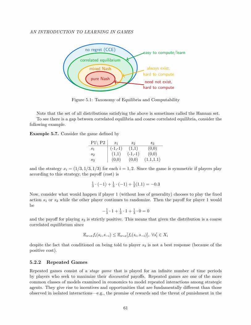
AN INTRODUCTION TO LEARNING IN GAMES
no regret (CCE)
pure Nash
mixed Nash
correlated equilibrium
need not exist,
hard to compute
always exist,
hard to compute
easy to compute/learn
Figure 5.1: Taxonomy of Equilibria and Computability
Note that the set of all distributions satisfying the above is sometimes called the Hannan set.To see there is a gap between correlated equilibria and coarse correlated equilibria, consider the
following example.
Example 5.7. Consider the game defined by
P1\ P2 s1 s2 s3
s1 (-1,-1) (1,1) (0,0)s2 (1,1) (-1,-1) (0,0)s3 (0,0) (0,0) (1.1,1.1)
and the strategy xi = (1/3, 1/3, 1/3) for each i = 1, 2. Since the game is symmetric if players playaccording to this strategy, the payoff (cost) is
13 · (−1) + 1
3 · (−1) + 13(1.1) = −0.3
Now, consider what would happen if player 1 (without loss of generality) chooses to play the fixedaction s1 or s2 while the other player continues to randomize. Then the payoff for player 1 wouldbe
−13 · 1 + 1
3 · 1 + 13 · 0 = 0
and the payoff for playing s3 is strictly positive. This means that given the distribution is a coarsecorrelated equilibrium since
Es∼xfi(si, s−i) ≤ Es∼x[fi(si, s−i)], ∀s′i ∈ Xi
despite the fact that conditioned on being told to player s3 is not a best response (because of thepositive cost).
5.2.2 Repeated Games
Repeated games consist of a stage game that is played for an infinite number of time periodsby players who seek to maximize their discounted payoffs. Repeated games are one of the morecommon classes of models examined in economics to model repeated interactions among strategicagents. They give rise to incentives and opportunities that are fundamentally different than thoseobserved in isolated interactions—e.g., the promise of rewards and the threat of punishment in the
61
AN INTRODUCTION TO LEARNING IN GAMES
future of the game can provide incentives for desirable behavior now. Moreover, repeated play givesplayers (and potentially incentive designers) the opportunity to learn and adapt their strategies.
In what follows, we will distinguish a bit between strategies and actions. Let G = X, (fi)i∈N denote the stage game. Players repeatedly play G at times t. Let hti denote the history observedby player i up to time t. Then, Ht
i is the set of all such histories at time t, and Hi = ∪tHti the set
of all histories over time. Then, a policy (or strategy) πi : Hi → Xi for player i is a mapping fromthe the set of histories to a mixed action (or even a pure action depending on the context).2 Inparticular, a strategy π = (π1, . . . , πN ) induces an sequence of (mixed) action profiles xtt. Thestrategy for player i takes in the history ht and generates an action xti for that player. That is,
πi(hti) = xti ∈ Xi
Let δ be the common discount factor for all players. The total cost for player i is then
Fi(πi, π−i) = (1− δ)∞∑t=1
δtfi(xti, x
t−i)
Classification of repeated games by available information. What information players haveavailable to them is crucial in determining the outcome of repeated games. There are several typesof information structures typically referred to as different types of monitoring:
• Perfect public monitoring: At the end of each time period t, players can observe eachothers’ actions and payoffs. With perfect public monitoring hti = ht for all i and ht =(x1, . . . , xt−1).
• Imperfect public monitoring: At the end of each time period t, players can only observe apublic signal that contains information about the other players’ actions, but this signal doesnot necessarily determine the opponents’ actions. That is, we have again that hti = ht for alli but ht is not necessarily equal to (x1, . . . , xt−1).
• Private monitoring: At the end of each time period t, players receive a possibly differentprivate signal containing information about what has happened in that round.
Note that one can relate this in the learning dynamics to coupled, uncoupled, and completelyuncoupled dynamics where coupling is used to mean information available.
Learning Algorithms as Strategies. Interestingly, we can think of the policy πi : Hi → Xi asan algorithm, and in the context of the learning in games literature this is precisely what peopletend to do. Here, an algorithms Ai selects a distribution xti
5.2.3 External Regret
To introduce the idea of regret in the context of repeated play games, we will consider algorithmsfor repeated play of a matrix game with the guarantee that against any opponent, they will performnearly as well as the best fixed action in hindsight. This is often called the problem of combiningexpert advice or minimizing external regret.
2We say mixed more generally here since it encompasses the possibility of pure actions.
62
AN INTRODUCTION TO LEARNING IN GAMES
To introduce this concept, we will start by taking the view of a single agent against an adversaryand hence, we do not add the i subscript here to the action set or actions. Consider a set X ofn ≥ 2 actions. At time each time t = 1, . . . , T , the following occurs:
• A decision maker picks a mixed strategy xt that is a distribution over its actions X.
• An adversary picks a cost vector `t : X → [0, 1].
• An actions st is chosen according to the distribution xt and the decision maker incurs a cost`t(st).
• The decision maker learns the entire cost vector `t not just the realized cost `t(st).
For example, one may consider X to be different investment strategies or different driving routesbetween home and work. And, the decision-maker tries to determine the least costly action amongstthose in X assuming worst case outcomes. In the multi-player setting (which we will get to), theaction set will be the strategy of a single player and the cost vector will be induced by the strategieschosen by all the other players.
Another noteworthy point is that a number of online convex optimization problems can be castin this decision-maker–adversary framework.
We seek a good algorithm for online decision-making problems of the above type. The perfor-mance of the algorithm is measured by
Regret(T ) = “Total profit of best fixed action in hindsight”− “Total profit of algorithm”
Definition 5.8 (Time Average Regret). The (time average) regret of the action sequence s1, . . . , sT
with respect to a fixed action s is given by
1
T
(T∑t=1
`t(st)−T∑t=1
`t(s)
)
Please note there are several other notions of regret including internal and swap regret that arecommonly used in analyzing learning in games. We will focus on external regret for now.
Let A be an online decision-making algorithm. An adversary for A is a function that takesas input the time index t, the mixed strategies (x1, . . . , xt) produced by A up to time t, and therealized actions s1, . . . , st−1 up to time t− 1. It produces as output, the cost vector `t : S → [0, 1].
Definition 5.9 (No-Regret Algorithm.). An online decision making algorithm A has no (external)regret if the expected regret with respect to every action s ∈ X is o(1)3 as T →∞ independent ofthe adversary—that is,
limT→∞
1
T
(T∑t=1
`t(st)−T∑t=1
`t(s)
)→ 0
meaning that the regret grows sublinearly in T .
3A function f ∈ O(g) means that for at least one constant k > 0, you can find a constant c such that 0 ≤ f(x) ≤kg(x) for all x > c. Note that f ∈ o(g) means that the above holds for every choice of k > 0. Big-O essentially saysthat f grows asymptotically no faster than g and Little-o says that the asymptotic growth of f is strictly slower thang. In particular, f ∈ o(g) means limx→∞
f(x)g(x)
= 0 while f ∈ O(g) means limx→∞f(x)g(x)
<∞.
63
AN INTRODUCTION TO LEARNING IN GAMES
If we think of each action as an “expert” that makes recommendations, then a no-regret al-gorithms performs asymptotically as well as the best expert. The adversary in the definition ofno-regret algorithms is sometimes called an adaptive adversary. As an alternative, an obliviousadversary is the special case in which the cost vector `t depends only on t (and on the algorithmA).
There are several notable results in the study of no-regret algorithms.
Theorem 5.10 (Informal). The following two results hold for no-regret algorithms.
1. No-regret Algorithms exist and they tend to be simple and have expected regret O(√
(lnn)/T )with respect to every fixed action (n is the number of actions).
2. There exists an online decision-making algorithm that, for every ε > 0, has expected regretat most ε with respect to every fixed action after O
((lnn)/ε2
)iterations.
The Multiplicative Weights (MW) algorithm (aka Randomized Weighted Majority or Hedge) isa no-regret algorithm. It maintains a weight, intuitively a “credibility,” for each action. At eachtime step the algorithm chooses an action with probability proportional to its current weight. Theweight of each action can only decrease, and the rate of decrease depends on the cost of the action.
The main idea comes from the following two formalisms:
1. Past performance of actions should guide which action is chosen now. Since the action choicemust be randomized, the probability of choosing an action should be increasing in its pastperformance (i.e., decreasing in its cumulative cost).
2. Many instantiations of the above idea yield no-regret algorithms. For optimal regret bounds,however, it is important to aggressively punish bad actions—i.e., when an action previouslyobserved to be ‘good’ turns out to be ‘bad’, the probability with which it is played shoulddecrease at an exponential rate.
Algorithm 1 Multiplicative Weights Sketch
1: procedure MW(T ) . final time2: w1(s)← 1, ∀s ∈ X3: for t = 1, . . . , T do4: xt = wt/Γt where Γt =
∑s∈X w
t(s) . compute current distribution5: Play an action s ∼ xt = . choose action and play6: Receive loss vector `t
7: For each s ∈ X, wt+1(s)← wt(s)(1− ε)`t(s) . update weights
In the above algorithm, e.g., if all losses are either 0 or 1 (a typical assumption), then the weightof each action either stays the same (if `t(s) = 0) or gets multiplied by (1− ε) (if `t(s) = 1).
As ε → 0, xt tends towards the uniform distribution and thus, small values of ε encourageexploration. As ε → 1, xt tends to the distribution that puts all its mass on the action that hasincurred the smallest cumulative cost so far and thus, large values of ε encourage “exploitation.”
5.2.4 No-Regret Dynamics in Games
We now go from single player with adversary to multi-player settings and do so in the cost mini-mization framework here.
For each time t = 1, 2, . . . , T , the following events occur:
64
AN INTRODUCTION TO LEARNING IN GAMES
1. Each player i simultaneously and independently chooses a mixed strategy xti using a no-regretalgorithm.
2. Each player i receives a cost vector `ti where `ti(si) is the expected cost of action si when theother players play their chosen mixed strategies—i.e.,
`ti(si) = Es−i∼x−i [fi(si, s−i)]
where x−i =∏j 6=i xj and fi is the cost function for agent i.
No-regret dynamics are well defined because no-regret algorithms exist (we did not prove thisbut we stated it earlier). It is very interesting to note that players do not have to use the sameno-regret algorithm; they just have to use some no-regret algorithm. In addition, while above wehave described the players moving simultaneously, the results also extend to players that movesequentially.
No-regret dynamics can be implemented efficiently. Indeed, consider multiplicative weightswhere n is the (maximum) size of a player’s strategy space (across players). Suppose each playeruses the multiplicative weights algorithm. Then in each iteration each player does a simple updateof one weight per strategy, and only O((lnn)/ε2) iterations of this are required before every playerhas expected regret at most ε for every strategy. This follows from the analysis in the single playersetting.
Perhaps most interestingly we can guarantee that no-regret dynamics converge to coarse corre-lated equilibria.
Proposition 5.11 (Convergence to CCE.). Suppose after T iterations of no-regret dynamics, everyplayer of a cost minimization game has regret at most ε for each of its strategies. Let xt =
∏Ni=1 x
ti
denote the distribution at time t and let x = 1T
∑Tt=1 x
t be the time averaged history of thesedistributions. Then x is an ε–approximate coarse correlated equilibrium in the sense that for eachi,
Es∼x[fi(s)] ≤ Es−i∼x−i [fi(s′i, s−i)] + ε ∀ s′i ∈ Xi
Proof. By definition, for each i
Es∼x[fi(a)] =1
T
T∑t=1
Es∼xt [fi(a)] (5.9)
and
Es−i∼x−i [fi(s′i, s−i)] =
1
T
T∑t=1
Es∼xt [fi(s′i, s−i)] (5.10)
(since x is the time average distribution). The right hand side of (5.9) and are the time averagedexpected costs of player i when playing according to its no-regret algorithm, and the right hand sideof (5.10) is the time averaged expected cost when playing the fixed actions s′i every time instance.By assumption every player has at most regret ε so that (5.9) is at most ε more than (5.10).
It is interesting to note that very simple learning algorithms lead remarkably quickly to (ap-proximate) coarse correlated equilibria. In this sense, coarse correlated equilibria are, perhapsunusually, tractable to compute, and hence unusually plausible as a prediction for player behavior.
65
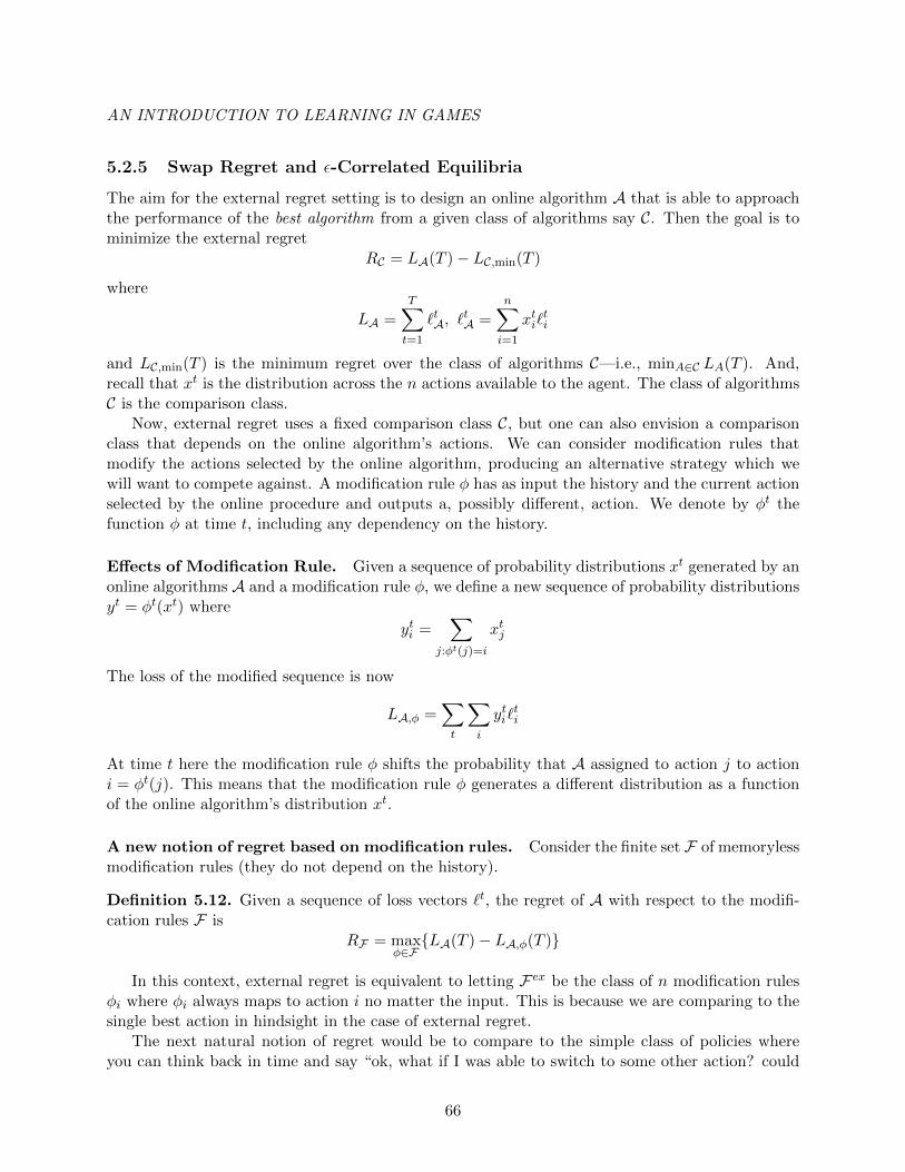
AN INTRODUCTION TO LEARNING IN GAMES
5.2.5 Swap Regret and ε-Correlated Equilibria
The aim for the external regret setting is to design an online algorithm A that is able to approachthe performance of the best algorithm from a given class of algorithms say C. Then the goal is tominimize the external regret
RC = LA(T )− LC,min(T )
where
LA =
T∑t=1
`tA, `tA =
n∑i=1
xti`ti
and LC,min(T ) is the minimum regret over the class of algorithms C—i.e., minA∈C LA(T ). And,recall that xt is the distribution across the n actions available to the agent. The class of algorithmsC is the comparison class.
Now, external regret uses a fixed comparison class C, but one can also envision a comparisonclass that depends on the online algorithm’s actions. We can consider modification rules thatmodify the actions selected by the online algorithm, producing an alternative strategy which wewill want to compete against. A modification rule φ has as input the history and the current actionselected by the online procedure and outputs a, possibly different, action. We denote by φt thefunction φ at time t, including any dependency on the history.
Effects of Modification Rule. Given a sequence of probability distributions xt generated by anonline algorithms A and a modification rule φ, we define a new sequence of probability distributionsyt = φt(xt) where
yti =∑
j:φt(j)=i
xtj
The loss of the modified sequence is now
LA,φ =∑t
∑i
yti`ti
At time t here the modification rule φ shifts the probability that A assigned to action j to actioni = φt(j). This means that the modification rule φ generates a different distribution as a functionof the online algorithm’s distribution xt.
A new notion of regret based on modification rules. Consider the finite set F of memorylessmodification rules (they do not depend on the history).
Definition 5.12. Given a sequence of loss vectors `t, the regret of A with respect to the modifi-cation rules F is
RF = maxφ∈FLA(T )− LA,φ(T )
In this context, external regret is equivalent to letting Fex be the class of n modification rulesφi where φi always maps to action i no matter the input. This is because we are comparing to thesingle best action in hindsight in the case of external regret.
The next natural notion of regret would be to compare to the simple class of policies whereyou can think back in time and say “ok, what if I was able to switch to some other action? could
66
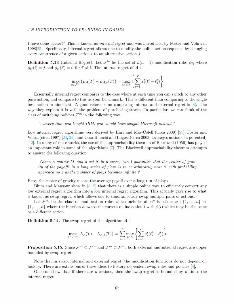
AN INTRODUCTION TO LEARNING IN GAMES
I have done better?” This is known as internal regret and was introduced by Foster and Vohra in1998[25]. Specifically, internal regret allows one to modify the online action sequence by changingevery occurrence of a given action i to an alternative action j.
Definition 5.13 (Internal Regret). Let F in be the set of n(n − 1) modification rules φij whereφij(i) = j and φij(i
′) = i′ for i′ 6= i. The internal regret of A is
maxφ∈Fin
LA(T )− LA,φ(T ) = maxi,j∈X
T∑t=1
xti(`ti − `tj)
Essentially internal regret compares to the case where at each time you can switch to any otherpure action, and compare to this as your benchmark. This is different than comparing to the singlebest action in hindsight. A good reference on comparing internal and external regret is [8]. Theway they explain it is with the problem of purchasing stocks. In particular, we can think of theclass of switching policies F in in the following way.
“...every time you bought IBM, you should have bought Microsoft instead.”
Low internal regret algorithms were derived by Hart and Mas-Colell (circa 2000) [29], Foster andVohra (circa 1997) [24, 25], and Cesa-Bianchi and Lugosi (circa 2003, leverages notion of a potential)[12]. In many of these works, the use of the approachability theorem of Blackwell (1956) has playedan important role in some of the algorithms [7]. The Blackwell approachability theorem attemptsto answer the following question:
Given a matrix M and a set S in n-space, can I guarantee that the center of grav-ity of the payoffs in a long series of plays is in or arbitrarily near S with probabilityapproaching 1 as the number of plays becomes infinite ?
Here, the center of gravity means the average payoff over a long run of plays.Blum and Mansour show in [8, 9] that there is a simple online way to efficiently convert any
low external regret algorithm into a low internal regret algorithm. This actually gave rise to whatis known as swap regret, which allows one to simultaneously swap multiple pairs of actions.
Let Fsw be the class of modification rules which includes all nn functions φ : 1, . . . , n →1, . . . , n where the function φ swaps the current online action i with φ(i) which may be the sameor a different action.
Definition 5.14. The swap regret of the algorithm A is
maxφ∈Fsw
LA(T )− LA,φ(T ) =
n∑i=1
maxj∈X
T∑t=1
xti(`ti − `tj)
Proposition 5.15. Since Fex ⊂ Fsw and F in ⊂ Fsw, both external and internal regret are upperbounded by swap regret.
Note that in swap, internal and external regret, the modification functions do not depend onhistory. There are extensions of these ideas to history dependent swap rules and policies [8],
One can show that if there are n actions, then the swap regret is bounded by n times theinternal regret.
67
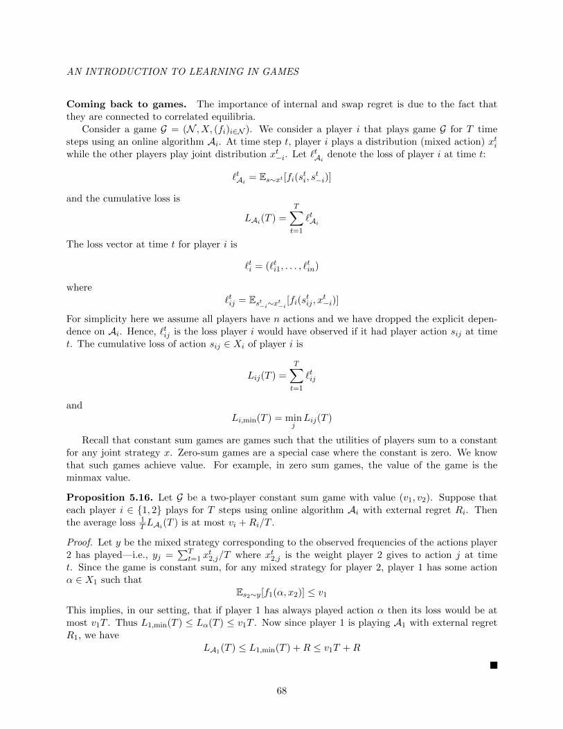
AN INTRODUCTION TO LEARNING IN GAMES
Coming back to games. The importance of internal and swap regret is due to the fact thatthey are connected to correlated equilibria.
Consider a game G = (N , X, (fi)i∈N ). We consider a player i that plays game G for T timesteps using an online algorithm Ai. At time step t, player i plays a distribution (mixed action) xtiwhile the other players play joint distribution xt−i. Let `tAi denote the loss of player i at time t:
`tAi = Es∼xt [fi(sti, st−i)]
and the cumulative loss is
LAi(T ) =
T∑t=1
`tAi
The loss vector at time t for player i is
`ti = (`ti1, . . . , `tin)
where`tij = Est−i∼xt−i [fi(s
tij , x
t−i)]
For simplicity here we assume all players have n actions and we have dropped the explicit depen-dence on Ai. Hence, `tij is the loss player i would have observed if it had player action sij at timet. The cumulative loss of action sij ∈ Xi of player i is
Lij(T ) =
T∑t=1
`tij
andLi,min(T ) = min
jLij(T )
Recall that constant sum games are games such that the utilities of players sum to a constantfor any joint strategy x. Zero-sum games are a special case where the constant is zero. We knowthat such games achieve value. For example, in zero sum games, the value of the game is theminmax value.
Proposition 5.16. Let G be a two-player constant sum game with value (v1, v2). Suppose thateach player i ∈ 1, 2 plays for T steps using online algorithm Ai with external regret Ri. Thenthe average loss 1
T LAi(T ) is at most vi +Ri/T .
Proof. Let y be the mixed strategy corresponding to the observed frequencies of the actions player2 has played—i.e., yj =
∑Tt=1 x
t2,j/T where xt2,j is the weight player 2 gives to action j at time
t. Since the game is constant sum, for any mixed strategy for player 2, player 1 has some actionα ∈ X1 such that
Es2∼y[f1(α, x2)] ≤ v1
This implies, in our setting, that if player 1 has always played action α then its loss would be atmost v1T . Thus L1,min(T ) ≤ Lα(T ) ≤ v1T . Now since player 1 is playing A1 with external regretR1, we have
LA1(T ) ≤ L1,min(T ) +R ≤ v1T +R
68
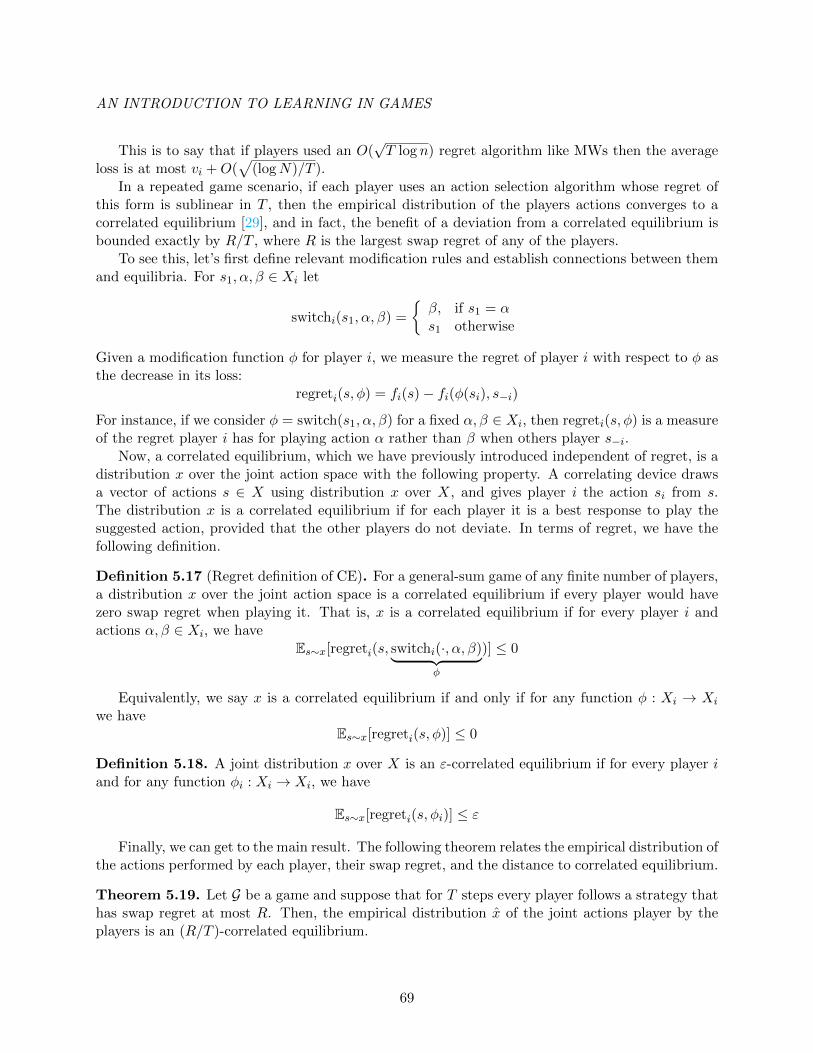
AN INTRODUCTION TO LEARNING IN GAMES
This is to say that if players used an O(√T log n) regret algorithm like MWs then the average
loss is at most vi +O(√
(logN)/T ).In a repeated game scenario, if each player uses an action selection algorithm whose regret of
this form is sublinear in T , then the empirical distribution of the players actions converges to acorrelated equilibrium [29], and in fact, the benefit of a deviation from a correlated equilibrium isbounded exactly by R/T , where R is the largest swap regret of any of the players.
To see this, let’s first define relevant modification rules and establish connections between themand equilibria. For s1, α, β ∈ Xi let
switchi(s1, α, β) =
β, if s1 = αs1 otherwise
Given a modification function φ for player i, we measure the regret of player i with respect to φ asthe decrease in its loss:
regreti(s, φ) = fi(s)− fi(φ(si), s−i)
For instance, if we consider φ = switch(s1, α, β) for a fixed α, β ∈ Xi, then regreti(s, φ) is a measureof the regret player i has for playing action α rather than β when others player s−i.
Now, a correlated equilibrium, which we have previously introduced independent of regret, is adistribution x over the joint action space with the following property. A correlating device drawsa vector of actions s ∈ X using distribution x over X, and gives player i the action si from s.The distribution x is a correlated equilibrium if for each player it is a best response to play thesuggested action, provided that the other players do not deviate. In terms of regret, we have thefollowing definition.
Definition 5.17 (Regret definition of CE). For a general-sum game of any finite number of players,a distribution x over the joint action space is a correlated equilibrium if every player would havezero swap regret when playing it. That is, x is a correlated equilibrium if for every player i andactions α, β ∈ Xi, we have
Es∼x[regreti(s, switchi(·, α, β)︸ ︷︷ ︸φ
)] ≤ 0
Equivalently, we say x is a correlated equilibrium if and only if for any function φ : Xi → Xi
we haveEs∼x[regreti(s, φ)] ≤ 0
Definition 5.18. A joint distribution x over X is an ε-correlated equilibrium if for every player iand for any function φi : Xi → Xi, we have
Es∼x[regreti(s, φi)] ≤ ε
Finally, we can get to the main result. The following theorem relates the empirical distribution ofthe actions performed by each player, their swap regret, and the distance to correlated equilibrium.
Theorem 5.19. Let G be a game and suppose that for T steps every player follows a strategy thathas swap regret at most R. Then, the empirical distribution x of the joint actions player by theplayers is an (R/T )-correlated equilibrium.
69
AN INTRODUCTION TO LEARNING IN GAMES
Proof. The empirical distribution x assigns to every xt a probability of 1/T . Fix a function φi :Xi → Xi for player i. Since player i has swap regret at most R, we have that
LAi(T ) ≤ LAi,φi(T ) +R
where LAi(T ) is the cumulative loss of player i. By the definition of the regret function, we have
LAi(T )− LAi,φi(T ) =T∑t=1
Est∼xt [fi(st)]−T∑t=1
Est∼xt [fi(φi(sti), st−i)]
=T∑t=1
Est∼xt [regreti(st, φi)]
= TEs∼x[regreti(s, φi)], since x = 1T x
t
Thus, for any φi : Xi → Xi, we have
Es∼x[regreti(s, φi)] ≤R
T
This results says that the payoff of each player is its payoff in some approximate correlatedequilibrium. In addition, it relates the swap regret to the distance from equilibrium. Note that ifthe average swap regret vanishes then the procedure converges, in the limit, to the set of correlatedequilibria.
5.3 Follow The Regularized Leader
We have not discussed how regret of algorithms connects to equilibrium concepts, but we havereally only mentioned one algorithm, namely Multiplicative Weights. The multiplicative weightsalgorithm is simple to define and analyze, and it has several applications, but perhaps it is notclear where this algorithm comes from. We saw briefly the connection to continuous time replicatordynamics. In fact it is connected to a more general class of learning dynamics known as follow theregularized leader.
The solution xt proposed by the algorithm at time t can only depend on the previous lossfunction `1, . . . , `t−1. But, the question is how should it depend on it? If the offline optimalsolution x is consistently better than all others at each time step, then we would like xt to bethat solution, so we want xt to be a solution that would have worked well in the previous steps.The most extreme way of implementing this idea is what is know as Follow the Leader algorithm(abbreviated FTL), in which we set the solution at time t to be
xt = arg minx∈X
t−1∑k=1
`k(x)
This algorithm can perform poorly, since it can easily overfit to the past data which itself may bebad. The way we fix this (and a common theme more generally in machine learning if we want toavoid overfitting and promote generalization) is to regularize. That is, we do not want the solutionto change much from round to round.
70
AN INTRODUCTION TO LEARNING IN GAMES
Consider the FTRL (follow the regularized leader) update
xt = arg minx∈X
r(x) +t−1∑k=1
`k(x)
Typically, the function r(·) is chosen to be strictly convex and to take values that are rather big inmagnitude.
Now consider a game setting in which each player is updating according to the above followthe regularized leader dynamics. These dynamics actually have an equivalent continuous timeformulation which has been recently studied in adversarial learning (and more generallly zero sumgames) [37]:
yi(t) = yi(0) +
∫ t
0vi(x(τ)) dτ (5.11)
xi(t) = Qi(yi(t)) (5.12)
whereui(x) = 〈vi(x), xi〉 =
∑αi∈Xi
xi,αivi,αi(x)
withvi(x) = (vi,αi(x))αi∈Xi
being the vector of payoffs to player i given they player strategy αi and the remaining players playmixed strategy x−i. In addition, Qi : R|Xi| → Xi is the choice map defined by
Qi(yi) = arg maxxi∈Xi
〈yi, xi〉 − ri(xi)
Suppose that r is continuous and strictly convex on Xi (for each i) and is smooth on the relativeinterior of every face of Xi including Xi itself. The choice map with the regularizer essentially actsto smooth the hard argmax correspondence yi 7→ arg maxxi∈Xi〈yi, xi〉.
As already alluded two the two quintessential examples of FTRL dynamics are multiplicativeweights (which we get by using the entroptic regularizer ri(x) =
∑αi∈Xi xi,αi log xiαi), and the
classical Euclidean projection dynamics which are induced by the regularizer ri(x) = 12‖xi‖
2.
Theorem 5.20. A player using FTRL has a O(1/T ) regret bound independent of what otherplayers do. That is, if a player i ∈ N follows FTRL then for every continuous trajectory x−i(t) ofthe opponents of player i, we have that
Regi(T ) ≤ Ω
T
where Ω = max ri −min ri is a positive constant.
Here the regret for the continuous time case is
Regi(T ) = maxzi∈X
1
T
∫ t
0(ui(zi, x−i(τ))− ui(x(τ))) dτ
71
Part III
Applications in Learning-BasedSystems and Market-Based AI
72
Chapter 6
Adversarial Learning
73
Chapter 7
Distributionally Robust Optimization
74
Chapter 8
Decision-making Using StrategicallyGenerated Data
75
Chapter 9
Multi-Agent Reinforcement Learning
76
Part IV
Appendices
77
Appendix A
Review of Function Properties
A.1 Preliminaries
Given a metric space X with metric ρ, we denote Br(x) as the r-radius ball around the point xusing the metric ρ. For example, if X = Rn is the n-dimensional Eucldiean space endowed with theusual Euclidean metric—i.e., the 2-norm—then B1(0) is the usual unit norm ball we are familiarwith.
The notation f ∈ Cr(X,R) to denote that a real-valued function f(x) belongs to the familyof r-continuously differentiable (sometimes referred to as r-smooth) on a space X functions. Ingeneral, throughout this set of lecture notes, we will take X ⊆ Rn.
A.2 Extrema of Functions and Classification of Critical Points
A very important thing to point out here:
There is a difference between critical points of functions and critical pointsof dynamical systems.
In this section, we focus on critical points of functions.For a function f ∈ C2(Rn,R), we define critical points as follows.
Definition A.1. A point x is a critical point of f if Df(x) = 0.
Critical points have different classifications. They can be (local) minima, (local) maxima, or(local) saddle points, the latter of which is sometimes referred to as a (local) minimax point. Inzero-sum games, e.g., we care about the subset of such saddle points whose defining saddle curvaturedirections are aligned with the players’ actions. These correspond to local minimax points for thegame—that is to say that not all saddle points of a function are game theoretically meaningful.
For a given function f ∈ C2(Rn,R), we define a local minima as follows.
Definition A.2. A point x∗ ∈ U ⊂ Rn is a local minimum for the function f ∈ C2(Rn,R) if
f(x∗) ≤ f(x), ∀x ∈ U
78
AN INTRODUCTION TO LEARNING IN GAMES
A local maximum is defined analogously. Sometimes the definition of a local extremal pointis defined given a metric on Rn. For example, a δ-local minima of f is a point x∗ such thatf(x∗) ≤ f(x) for all x ∈ Bδ(x∗). Another way you may encounter a local minima is as follows: apoint x∗ is a local minima if there exists a δ > 0 such that f(x∗) ≤ f(x) for all x ∈ Bδ(x∗).
The last important critical point type is a saddle point.
Definition A.3. A critical point x—i.e., Df(x) = 0—is a saddle point of f if f does not have alocal extremum at x∗.
Here, a local extremum is either a local maximum or a local mimimum.From calculus, you should remember that second order conditions can be used to determine the
existence of a local extremum at a critical point.
Proposition A.4. A critical point x∗ of the function f ∈ C2(Rn,R) is a
1. local maximum if D2f(x∗) < 0—i.e., the matrix D2f(x∗) is strictly negative definite.
2. local minimum if D2f(x∗) > 0—i.e., the matrix D2f(x∗) is strictly positive definite.
Note that these are sufficient conditions. There are also necessary conditions.
Proposition A.5. If a critical point x∗ of the function f ∈ C2(Rn,R) is a local minimum, thenD2f(x∗) ≥ 0. Analogously, if a critical point x∗ of the function f ∈ C2(Rn,R) is a local maximum,then D2f(x∗) ≤ 0
It is a generic property of the function f ∈ C2(Rn,R) that any local minima x∗ (resp. localmaxima) satisfies D2f(x∗) < 0 (resp. D2f(x∗) > 0). That is, generically the sufficient conditionsof Proposition A.4 are also necessary. This means that for almost all (in a formal mathematicalsense) sufficiently smooth functions, the second order test in Proposition A.4 is both necessary andsufficient. Moreover, this is a structurally stable property, meaning that if we have a critical pointx∗ that is a local extremum, then it persists under smooth perturbations of the function. Thisbeing said, there are functions that define important classes of games which do not possess thisgeneric property. That is, they belong to a measure zero set of functions. For instance, bilinearfunctions such as x>y define the class of bilinear games, and the extrema of this type of functiondoes not have the generic property described above.
Returning back to the discussion of saddle points, we also define the strict saddle property.
Definition A.6. A critical point x∗ of the function f ∈ C2(Rn,R) is a strict saddle point of f if ithas both a strictly negative eigenvalue and a strictly positive eigenvalue—that is, λmin(D2f(x∗)) < 0and λmax(D2f(x∗)) > 0 where λmin(·) and λmax(·) denote the minimum and maximum eigenvalueof their argument, respectively.
A.3 Convexity
79
Appendix B
Review of Dynamical Systems Theory
B.1 Motivation for the Use of Dynamical Systems Theory
To understand convergence or recurrence properties, learning in games requires the use of dynamicalsystems theory. This is unlike gradient descent in optimization (a single player game) for which wehave a number of tools that are parallel to those in dynamical systems theory.
This is because gradient descent in optimization corresponds to gradient flow. For example,consider the objective of minimizing the function f ∈ C2(Rn,R):
minxf(x)
In general, f(x) is non-convex in x (cf. Appendix A for a review of function properties), meaningthat we seek local minma of this function. Towards finding local minima, one natural scheme is tofollow the gradient of
Beyond gradient descent, however, even more complex algorithms for single player optimizationsuch as momentum-based or symplectic algorithms used, for example, to speed up convergenceoften require dynamical systems theory and numerical methods for ordinary differential equations(odes). Hence, we will review some basics of numerical methods for odes, focusing primarily onfirst order methods.
B.2 Review of Numerical Methods for Differential Equations
80
Appendix C
Dynamic Games
81
Appendix D
Mechanism Design
82
Bibliography
[1] Ilan Adler. The equivalence of linear programs and zero-sum games. International Journal ofGame Theory, 42(1):165–177, 2013.
[2] Sanjeev Arora, Elad Hazan, and Satyen Kale. The multiplicative weights update method: ameta-algorithm and applications. Theory of Computing, 8(1):121–164, 2012.
[3] Robert J Aumann. Subjectivity and correlation in randomized strategies. Journal of mathe-matical Economics, 1(1):67–96, 1974.
[4] Didier Aussel and Joydeep Dutta. Generalized nash equilibrium problem, variational inequalityand quasiconvexity. Operations research letters, 36(4):461–464, 2008.
[5] Tamer Basar and Geert Jan Olsder. Dynamic noncooperative game theory. SIAM, 1998.
[6] Dimitri P Bertsekas, WW Hager, and OL Mangasarian. Nonlinear programming. AthenaScientific Belmont, MA, 1998.
[7] David Blackwell et al. An analog of the minimax theorem for vector payoffs. Pacific Journalof Mathematics, 6(1):1–8, 1956.
[8] Avrim Blum and Yishay Mansour. From external to internal regret. Journal of MachineLearning Research, 8(6), 2007.
[9] Blum, Avrim and Mansour, Yishay. Learning, Regret Minimization and Equilibria. 2007.
[10] Stephen Boyd, Stephen P Boyd, and Lieven Vandenberghe. Convex optimization. Cambridgeuniversity press, 2004.
[11] George W Brown. Iterative solution of games by fictitious play. Activity analysis of productionand allocation, 13(1):374–376, 1951.
[12] Nicolo Cesa-Bianchi and Gabor Lugosi. Potential-based algorithms in on-line prediction andgame theory. Machine Learning, 51(3):239–261, 2003.
[13] George Bernard Dantzig. Linear programming and extensions, volume 48. Princeton universitypress, 1998.
[14] Constantinos Daskalakis, Paul W Goldberg, and Christos H Papadimitriou. The complexityof computing a nash equilibrium. SIAM Journal on Computing, 39(1):195–259, 2009.
83
AN INTRODUCTION TO LEARNING IN GAMES
[15] Constantinos Daskalakis, Stratis Skoulakis, and Manolis Zampetakis. The complexity of con-strained min-max optimization. arXiv preprint arXiv:2009.09623, 2020.
[16] Gerard Debreu. A social equilibrium existence theorem. Proceedings of the National Academyof Sciences, 38(10):886–893, 1952.
[17] Yu G Evtushenko. Iterative methods for solving minimax problems. USSR ComputationalMathematics and Mathematical Physics, 14(5):52–63, 1974.
[18] Yu.G. Evtushenko. Some local properties of minimax problems. USSR Computational Math-ematics and Mathematical Physics, 14(3):129 – 138, 1974.
[19] Alex Fabrikant, Christos Papadimitriou, and Kunal Talwar. The complexity of pure nashequilibria. In Proceedings of the thirty-sixth annual ACM symposium on Theory of computing,pages 604–612, 2004.
[20] Francisco Facchinei and Christian Kanzow. Generalized nash equilibrium problems. Annalsof Operations Research, 175(1):177–211, 2010.
[21] Francisco Facchinei and Jong-Shi Pang. Finite-dimensional variational inequalities and com-plementarity problems. Springer Science & Business Media, 2007.
[22] Ky Fan. Fixed-point and minimax theorems in locally convex topological linear spaces. Pro-ceedings of the National Academy of Sciences of the United States of America, 38(2):121, 1952.
[23] Tanner Fiez, Benjamin Chasnov, and Lillian Ratliff. Implicit learning dynamics in Stackelberggames: Equilibria characterization, convergence analysis, and empirical study. In InternationalConference on Machine Learning (ICML), pages 3133–3144. PMLR, 2020.
[24] Dean P Foster and Rakesh V Vohra. Calibrated learning and correlated equilibrium. Gamesand Economic Behavior, 21(1-2):40, 1997.
[25] Dean P Foster and Rakesh V Vohra. Asymptotic calibration. Biometrika, 85(2):379–390, 1998.
[26] Ian Gemp and Sridhar Mahadevan. Online monotone games. arXiv preprint arXiv:1710.07328,2017.
[27] Itzhak Gilboa and Eitan Zemel. Nash and correlated equilibria: Some complexity considera-tions. Games and Economic Behavior, 1(1):80–93, 1989.
[28] Irving L Glicksberg. A further generalization of the kakutani fixed point theorem, with applica-tion to nash equilibrium points. Proceedings of the American Mathematical Society, 3(1):170–174, 1952.
[29] Sergiu Hart and Andreu Mas-Colell. A simple adaptive procedure leading to correlated equi-librium. Econometrica, 68(5):1127–1150, 2000.
[30] Sergiu Hart and Andreu Mas-Colell. Uncoupled dynamics do not lead to nash equilibrium.American Economic Review, 93(5):1830–1836, 2003.
[31] Josef Hofbauer, Karl Sigmund, et al. Evolutionary games and population dynamics. Cambridgeuniversity press, 1998.
84
AN INTRODUCTION TO LEARNING IN GAMES
[32] Chi Jin, Praneeth Netrapalli, and Michael Jordan. What is local optimality in nonconvex-nonconcave minimax optimization? In International Conference on Machine Learning(ICML), pages 4880–4889. PMLR, 2020.
[33] Ker-I Ko and Chih-Long Lin. On the complexity of min-max optimization problems and theirapproximation. In Minimax and Applications, pages 219–239. Springer, 1995.
[34] Thodoris Lykouris, Vasilis Syrgkanis, and Eva Tardos. Learning and efficiency in games withdynamic population. In Proceedings of the twenty-seventh annual ACM-SIAM symposium onDiscrete algorithms, pages 120–129. SIAM, 2016.
[35] Oren Mangoubi and Nisheeth K Vishnoi. A second-order equilibrium in nonconvex-nonconcavemin-max optimization: Existence and algorithm. arXiv preprint arXiv:2006.12363, 2020.
[36] Eric V Mazumdar, Michael I Jordan, and S Shankar Sastry. On finding local Nash equilibria(and only local Nash equilibria) in zero-sum games. arXiv preprint arXiv:1901.00838, 2019.
[37] Panayotis Mertikopoulos, Christos Papadimitriou, and Georgios Piliouras. Cycles in adversar-ial regularized learning. In Proceedings of the Twenty-Ninth Annual ACM-SIAM Symposiumon Discrete Algorithms, pages 2703–2717. SIAM, 2018.
[38] Panayotis Mertikopoulos and Zhengyuan Zhou. Learning in games with continuous action setsand unknown payoff functions. Mathematical Programming, 173(1-2):465–507, 2019.
[39] Dov Monderer and Lloyd S Shapley. Potential games. Games and economic behavior,14(1):124–143, 1996.
[40] John Nash. Non-cooperative games. Annals of Mathematics, 54(2):286–295, 1951.
[41] John F. Nash. Equilibrium points in n-person games. Proceedings of the National Academy ofSciences, 36(1):48–49, 1950.
[42] Martin J Osborne and Ariel Rubinstein. A course in game theory. MIT press, 1994.
[43] Christos H Papadimitriou and Tim Roughgarden. Computing correlated equilibria in multi-player games. Journal of the ACM (JACM), 55(3):1–29, 2008.
[44] TES Raghavan. Zero-sum two-person games. Handbook of game theory with economic appli-cations, 2:735–768, 1994.
[45] Lillian J Ratliff, Samuel A Burden, and S Shankar Sastry. Characterization and computationof local Nash equilibria in continuous games. In Allerton Conference on Communication,Control, and Computing (Allerton), pages 917–924, 2013.
[46] Robert W Rosenthal. A class of games possessing pure-strategy nash equilibria. InternationalJournal of Game Theory, 2(1):65–67, 1973.
[47] Florian Schafer and Anima Anandkumar. Competitive gradient descent. arXiv preprintarXiv:1905.12103, 2019.
[48] Sylvain Sorin. Replicator dynamics: Old and new. Journal of Dynamics & Games, 7(4):365,2020.
85
AN INTRODUCTION TO LEARNING IN GAMES
[49] Eva Tardos. Learning in games with dynamic population. Simons Institute Lecture: link toslides, 2015.
[50] Tatiana Tatarenko and Maryam Kamgarpour. Learning generalized nash equilibria in a classof convex games. IEEE Transactions on Automatic Control, 64(4):1426–1439, 2018.
[51] Tatiana Tatarenko and Maryam Kamgarpour. Learning nash equilibria in monotone games.In 2019 IEEE 58th Conference on Decision and Control (CDC), pages 3104–3109. IEEE, 2019.
[52] Heinrich Von Stackelberg. Market structure and equilibrium. Springer Science & BusinessMedia, 2010.
86